Phase diagram and dispersion relation of the non-commutative $\lambda\phi^{4}$ model in $d=3$

Abstract:

We present a non-perturbative study of the $\lambda\phi^{4}$ model in a three dimensional euclidean space, where the two spatial coordinates are non-commutative. Our results are obtained from numerical simulations of the lattice model, after its mapping onto a dimensionally reduced, twisted hermitean matrix model. In this way we first reveal the explicit phase diagram of the non-commutative $\lambda\phi^{4}$ lattice model. We observe that the ordered regime splits into a phase of uniform order and a phase of two stripes of opposite sign, and more complicated patterns. Next we discuss the behavior of the spatial and temporal correlators. From the latter we extract the dispersion relation, which allows us to introduce a dimensionful lattice spacing. To extrapolate to zero lattice spacing and infinite volume we perform a double scaling limit, which keeps the non-commutativity tensor constant. The dispersion relation in the disordered phase stabilizes in this limit, which represents a non-perturbative renormalization. In particular this confirms the existence of a striped phase in the continuum limit, in accordance with a conjecture by Gubser and Sondhi. The extrapolated dispersion relation also exhibits UV/IR mixing as a non-perturbative effect. Finally we add some observations about a Nambu-Goldstone mode in the striped phase, and about the corresponding model in $d=2$.

1 Non-commutative field theory

The idea of introducing non-commutative (NC) coordinate operators — or a spatial uncertainty — dates back to private communications involving Heisenberg, Peierls, Pauli and Oppenheimer. The coordinates are then given by hermitean operators $\hat{x}_{\mu}$ obeying a commutation relation of the form

$$[\hat{x}_{\mu},\hat{x}_{\nu}]=i\Theta_{\mu\nu}\,.$$ (1)

The first papers on this idea appeared in 1947 on quantum theory in flat [1] and curved [2] NC spaces. However, it was only at the end of the twentieth century that it attracted attention on a large scale in particle physics. Meanwhile, the mathematical foundation for quantum field theories on a NC space, NC field theories, was worked out; for an overview see refs. [3]. First applications using this type of space as a formalism — rather than a possible description of nature — emerged from solid state physics, see for instance refs. [4]. Nowadays also the possible reality of a NC space is a subject of intensive research.

It was string theory that finally boosted this field by identifying strings in certain low energy limits with NC field theory [5]. This was the main reason why NC field theory became extremely fashionable over the last years, so that more than $1300$ papers have been produced on it up to now [6]. We also take string theory as a motivation for our study, but in this work we investigate a NC field theory as such, without working out possible connections to other branches of physics.

A deep qualitative difference from ordinary (commutative) field theory is the occurrence of a non-locality of the range $\sqrt{\|\Theta\|}$. This property obviously implies conceptual problems, but from the optimistic point of view it may just provide the crucial link to string theory or to quantum gravity. In fact, there are arguments that a conciliation of gravity and quantum theory induces some sort of non-commutativity under quite general assumptions [7]. This line of thought would naturally include the time into the non-commutativity relation (1). However, in that setting the problems related to causality and unitarity are especially bad [8]. According to refs. [9] unitarity is on safe grounds for the Minkowski signature, but it is not yet clarified if the transition from a Euclidean to a Minkowski signature can be justified. For such reasons, much of the literature excludes time from the non-commutativity. This will also be our framework, since the use of a Euclidean space is vital for our numerical techniques, which will be explained below.

In the early days people hoped for yet another possible virtue due to the non-locality, namely that it would weaken or even remove the UV divergences of the commutative field theories [1], and therefore simplify the renormalization. This hope was badly disappointed: first it turned out that only part of the UV divergences are removed whereas others remain. In particular the UV divergences in the planar diagrams tend to survive the introduction of $\Theta$ [10]. What makes the situation much worse, however, is that the remaining commutative UV divergences do not just disappear, but they are typically converted into some kind of IR divergences. So one ends up with a troublesome mixing of divergences at both ends of the spectrum, denoted as UV/IR mixing [11]. A simple intuitive picture of this effect based on the uncertainty principle is described for instance in ref. [12]. We are going to illustrate the structure of such “mixed” divergences with an example in subsection 1.1. Beyond one loop, perturbation theory does not yet provide any systematic machinery to handle this type of divergences, which is unknown in commutative field theory. Hence adopting a fully non-perturbative approach is highly motivated, and this is the goal of the work presented here.

One issue that immediately arises is the question if UV/IR mixing is a technical problem of perturbation theory, or if it should rather be considered as a fundamental property of many NC field theories. Our previous numerical investigation of 2d NC $U(1)$ gauge theory clearly supported the latter point of view [16], in agreement with theoretical arguments [17]. Manifestations of UV/IR mixing can also be observed beyond perturbation theory — as the present work will demonstrate again — hence such mixing effects belong to the very nature of the corresponding NC models. This implies, for instance, that it is not promising to try to avoid such effects by performing some non-standard perturbative expansion (as it has been suggested occasionally in the literature).

In this work we consider the simplest case of an NC plane with a constant non-commutativity tensor, i.e. we deal with the non-commutativity of only two coordinates. Its extent is characterized by the parameter $\vartheta$,

$$[\hat{x}_{i},\hat{x}_{j}]=i\,\vartheta\,\epsilon_{ij}\,,\qquad i,j\in\{1,2\}\,,$$ (2)

where $\epsilon$ is the antisymmetric unit tensor. In addition we have a Euclidean time coordinate $t$. The whole 3d space is lattice discretized with equidistant lattice spacings. This is done by the standard procedure for the time coordinate, while we follow the instruction of refs. [17] for the NC plane. There we impose the operator equation

$$\exp\Big{(}i\frac{2\pi}{a}\hat{x}_{j}\Big{)}=\hat{\mathbbm{1}}\,,$$ (3)

where $a$ is the spatial lattice constant. Thus the spatial lattice sites are somewhat fuzzy. In our formulation the momentum components $p_{j}$ commute, and we have the usual periodicity over the Brillouin zone,

$$\exp\left(i\left[p_{j}+\frac{2\pi}{a}\right]\hat{x}_{j}\right)=\exp(ip_{j}\hat{x}_{j})\,.$$ (4)

Multiplication by a factor $\exp(-i\sum_{\ell=1}^{2}p_{\ell}\hat{x}_{\ell})$ leads to the condition

$$\frac{1}{2a}\,\vartheta\,p_{j}\in\mathbb{Z}\,.$$ (5)

Hence our NC lattice at fixed $\vartheta$ is automatically periodic.

Let us assume now that we are dealing with a torus of lattice size $N\times N$: then the momenta can take the discrete values

$$p^{(n)}=\frac{2\pi}{aN}\,n\,,\qquad n=(n_{1},n_{2})\,,\qquad n_{j}=1,\dots,N\,.$$ (6)

Together with relation (5) we identify the non-commutativity parameter as

$$\vartheta=\frac{1}{\pi}Na^{2}\,.$$ (7)

Taking the continuum limit of a NC theory requires to keep $\vartheta$ finite. By condition (7), the continuum limit $a\to 0$ and the thermodynamic limit $N\to\infty$ are entangled; we will take them simultaneously in such a way that the product $Na^{2}$ remains constant. Then obviously also the physical volume diverges. This kind of limit is denoted as the double scaling limit, and the entanglement that it involves is related to the UV/IR mixing: based on relation (7) we have to take the UV limit and the IR limit simultaneously.

1.1 The non-commutative $\lambda\phi^{4}$ model

NC field theories can be formulated in a form which looks similar to their commutative counterpart, if all field multiplications are performed by the star product [19]

$$\phi(x)\star\psi(x):=\phi(x)\exp\left(\frac{i}{2}\overleftarrow{\partial_{\mu}}\Theta_{\mu\nu}\overrightarrow{\partial_{\nu}}\right)\psi(x)\,,$$ (8)

as we recognize if the fields are decomposed into plane waves; a derivation is sketched in appendix A. Then we can work with ordinary coordinates $x_{\mu}$, and the non-commutativity is encoded in the star product.

In the specific case of bilinear terms in the action, the star product is equivalent to the ordinary product, as we see from integration by parts and the antisymmetry of the tensor $\Theta$. Equipped with these rules we can write down the action of the NC $\lambda\phi^{4}$ model in the $d$-dimensional Euclidean space,

$$S[\phi]=\int d^{d}x\,\left[\frac{1}{2}\partial_{\mu}\phi(x)\partial_{\mu}\phi(x)+\frac{m^{2}}{2}\phi(x)^{2}+\frac{\lambda}{4}\phi(x)\star\phi(x)\star\phi(x)\star\phi(x)\right].$$ (9)

We see that the strength of the self-interaction $\lambda$ also determines the extent of the effects due to the non-commutativity.

To illustrate now the UV/IR mixing — that we mentioned before — we consider the perturbative expansion of the one particle irreducible two-point function,

$$\Gamma(p)=\langle\tilde{\phi}(p)^{*}\tilde{\phi}(p)\rangle_{1PI}=\sum_{\ell=0}^{\infty}\lambda^{\ell}\Gamma^{(\ell)}(p)\,,$$ (10)

where $\tilde{\phi}$ is the scalar field in momentum space. To the leading order $\ell=0$ the action is bilinear, hence the star product is not needed and we find for the free field the same result as in the commutative case, $\Gamma^{(0)}(p)=p^{2}+m^{2}$. However, if we move on to $\Gamma^{(1)}$ the commutative term splits into a planar contribution, which is not affected by $\Theta$, plus a non-planar term, which is altered by the non-commutativity, $\Gamma^{(1)}(p)=\Gamma^{(1)}_{\rm p}+\Gamma^{(1)}_{\rm np}(p)$,

$$\Gamma^{(1)}_{\rm p}=2\int\frac{d^{d}q}{(2\pi)^{d}}\frac{1}{q^{2}+m^{2}}\,,\quad\Gamma^{(1)}_{\rm np}(p)=\int\frac{d^{d}q}{(2\pi)^{d}}\frac{\exp(iq_{\mu}\Theta_{\mu\nu}p_{\nu})}{q^{2}+m^{2}}\,.$$ (11)

The planar term confirms that part of the commutative UV divergences persist. It has been shown that this behavior holds for the planar terms to all orders [10, 11].

The non-planar term can be evaluated for instance with the Pauli-Villars regularization. In $d=4$ one obtains [11, 12]

$$\Gamma^{(1)}_{\rm np}(p)=\frac{1}{96\pi^{2}}\left[\Lambda_{\rm eff}^{2}-m^{2}\log\left(\frac{\Lambda_{\rm eff}^{2}}{m^{2}}\right)+O(1)\right]\,,\qquad\Lambda_{\rm eff}^{2}=\frac{1}{\frac{1}{\Lambda^{2}}-p_{\mu}\Theta_{\mu\nu}p_{\nu}}\,.$$ (12)

$\Lambda$ is the usual momentum cutoff as it appears in the commutative model and in the planar term of eq. (11). Eq. (12) shows explicitly that $\Gamma^{(1)}_{\rm np}(p)$ is UV finite (with respect to $\Lambda$) in the NC model at finite external momentum $p$. It diverges, however, if we take in addition the IR limit $p\to 0$, or the limit $\Theta\to 0$.

A step beyond standard perturbation theory in the discussion of the NC $\lambda\phi^{4}$ model was undertaken by Gubser and Sondhi, who performed a self-consistent Hartree-Fock type one-loop calculation [20]. This method would be exact for the $O(N)$ symmetric $\sigma$-model in the large $N$ limit. Gubser and Sondhi conjectured its (qualitative) applicability also at $N=1$. In particular they derived a prediction for the qualitative feature of the phase diagram. A strongly negative coefficient $m^{2}$ corresponds to a very low temperature, such that some ordered structure is enforced.

In dimensions $d=3$ and $4$, with two NC coordinates obeying eq. (2), ref. [20] predicted that

• at small $\vartheta$, decreasing $m^{2}$ results in the usual Ising type uniform order, as in the commutative model

• at larger values of $\vartheta$ the ordering favors the formation of stripes in some direction, where $\phi(x)$ takes opposite signs, or even the superposition of stripes in different directions (“checker board patterns”).

The phenomenon of a spontaneous stripe formation is also known in solid state physics, see for instance ref. [21]. However, such a phase is unknown in the commutative $\lambda\phi^{4}$ model. Its predicted appearance can be understood as a consequence of an IR divergence, which shifts the energy minimum to non-vanishing momenta. At $m^{2}\ll 0$ the modes close to the energy minimum may condense, which corresponds to the stabilization of such stripe patterns.

The conjecture by Gubser and Sondhi was later supported by a study using an effective action, which was treated approximately by the Raileigh-Ritz method [22]. The possible existence of this striped phase was also discussed in the framework of a renormalization group analysis in $4-\varepsilon$ dimensions [23]. For generalities on the wilsonian renormalization group in NC field theory, see refs. [24].

However, this new phase remained on the level of conjectures until the system could be studied non-perturbatively by means of Monte Carlo simulations. The explicit result for the phase diagram and for the dispersion relation on the 3d lattice, including its limit to the continuum and to infinite volume, will be presented here. Some points of this work have been anticipated in various proceeding contributions [25] and in a Ph.D. thesis [26].

We note that the occurrence of a striped phase implies the spontaneous breaking of translation and rotation invariance. The properties of the Nambu-Goldstone boson related to the broken translation symmetry will be discussed in section 8. Based on this symmetry breaking, Gubser and Sondhi did not expect a striped phase in $d=2$. However, it was observed numerically that a striped phase does exist in two dimensions [27], and we are going to confirm that observation in appendix B. As ref. [27] pointed out, this does not contradict the Mermin-Wagner Theorem [28], since the proof for that Theorem assumes properties like locality and a regular IR behavior, which do not hold in most NC field theories.

2 The matrix model formulation

A lattice formulation of the model (9) is obtained from the discretization as described in section 1, where the derivatives can be replaced (for instance) by differences between nearest neighbor lattice sites. However, in such a formulation the field variables on any two lattice sites are coupled through the star product. This property would make a direct simulation very tedious.

A way out of this problem is the mapping of the lattice model onto a dimensionally reduced, twisted matrix model. This procedure was suggested in refs. [17], as a refinement of a previous work on NC gauge theories in the continuum [29]. Some aspects of this map are summarized in appendix A.

For our scalar field $\phi(\vec{x},t)$ on a periodic lattice of size $N^{2}\times T$ and unit lattice spacing, this mapping leads to the action

$$S[\hat{\phi}]\!=\!N\mathop{\rm Tr}\nolimits\sum_{t=1}^{T}\left[\frac{1}{2}\sum_{j=1}^{2}\left(\hat{\Gamma}_{j}\hat{\phi}(t)\hat{\Gamma}_{j}^{\dagger}-\hat{\phi}(t)\right)^{2}+\frac{1}{2}\left(\hat{\phi}(t+1)-\hat{\phi}(t)\right)^{2}+\frac{m^{2}}{2}\hat{\phi}(t)^{2}+\frac{\lambda}{4}\hat{\phi}(t)^{4}\right],$$ (13)

where $\hat{\phi}(t)$ represents a hermitean $N\times N$ matrix, living on one of the discrete time points $t=1,\dots,T$.

Since the time direction is commutative, its contribution to the kinetic term can be discretized in the usual way. On the other hand, in the spatial directions the shift by one lattice unit has to be arranged for by some matrix transformation, in our case by the multiplication with the twist eaters $\hat{\Gamma}_{j}$. The condition for them is that they obey the ’t Hooft-Weyl algebra

$$\hat{\Gamma}_{i}\hat{\Gamma}_{j}={\cal Z}_{ji}\hat{\Gamma}_{j}\hat{\Gamma}_{i}\,,$$ (14)

where the phase factor ${\cal Z}_{ji}={\cal Z}_{ij}^{*}$ is the twist.

In general a phase factor like ${\cal Z}_{12}$ in a twisted matrix model can take the form [30]

$${\cal Z}_{12}=e^{2\pi ik/N}\,,\quad k\in\mathbb{Z}\,,$$ (15)

since the twist originates from the boundary conditions before compactification. In our formulation we set

$$k=\frac{N+1}{2}\,,$$ (16)

as we are going to explain in subsection 2.1. Thus our twist differs from the conventional choice $k=1$. Of course, this means that we have to use odd values for $N$. With this choice, the 3d lattice model and the 1d twisted matrix model (where the twist appears implicitly in the form of the twist eaters) can be rigorously identified [17] by means of Morita equivalence [31], which means that the algebras in both formulations are identical.

Note that typical matrices $\hat{\phi}(t)$ are densely filled. This is in contrast to ordinary lattice field theory simulations, where the matrices that appear upon integrating out some of the fields tend to be sparse. Hence the matrix multiplications in action (13) require a considerable computational effort (it grows as $O(N^{3})$, i.e. faster than the system size of $O(N^{2})$), since the standard lattice techniques for matrix operations cannot be applied. For a description of our numerical methods we refer to appendix C. At this point we only remark that the property of densely filled matrices can be considered as a problem inherited from the star products in the lattice action, though the mapping onto the matrix model still simplifies the simulation drastically.

2.1 The twist

Let us briefly discuss in this subsection our choice of the twist factor. It is instructive to return to a general spatial lattice constant $a$ in this context. First, since we are on a torus we should not use the unbounded operators $\hat{x}_{j}$. Instead we introduce the unitary matrices

$$\hat{Z}_{j}:=\exp\left(\frac{2\pi}{Na}i\hat{x}_{j}\right),$$ (17)

which obey the commutation relation

$$\hat{Z}_{i}\hat{Z}_{j}=\exp\left(-\frac{4\pi^{2}}{N^{2}a^{2}}i\Theta_{ij}\right)\hat{Z}_{j}\hat{Z}_{i}=\exp\left(-\frac{4\pi}{N}i\epsilon_{ij}\right)\hat{Z}_{j}\hat{Z}_{i}\,.$$ (18)

In the last step we have used the relations (2) and (7).

In order to describe the shift by one lattice unit we need the translation operator

$$\hat{D}_{j}:=e^{a\hat{\partial}_{j}}\,;$$ (19)

the operator $\hat{\partial}_{j}$ is introduced in appendix A. To perform this shift correctly, $\hat{D}_{j}$ has to fulfill the relation

$$\hat{D}_{j}\hat{Z}_{i}\hat{D}_{j}^{\dagger}=e^{2\pi ia\delta_{ij}/N}\hat{Z}_{i}\,.$$ (20)

The issue is now to find a matrix solution for the conditions (18) and (20). To this end we use the unitary twist eaters

$$\hat{\Gamma}_{1}=\pmatrix{0&1&&&&&\cr&0&1&&&&\cr&&.&.&&&\cr&&&.&.&&\cr&&&&.&.&\cr&&&&&0&1\cr 1&&&&&&0},\qquad\hat{\Gamma}_{2}=\pmatrix{1&&&&&&\cr&{\cal Z}_{21}&&&&&\cr&&{\cal Z}_{21}^{2}&&&&\cr&&&{\cal Z}_{21}^{3}&&&\cr&&&&.&&\cr&&&&&.&\cr&&&&&&},$$ (21)

where ${\cal Z}_{12}={\cal Z}_{21}^{*}$ characterizes the twist. Now we see that the ansatz

$$\hat{D}_{j}=\hat{\Gamma}_{j}\,,\qquad\hat{Z}_{1}=\hat{\Gamma}_{2}^{(N+1)/2}\,,\qquad\hat{Z}_{2}=\hat{\Gamma}_{1}^{\dagger~{}(N+1)/2}$$ (22)

does indeed solve the conditions (18) and (20) for odd $N$, iff the twist has the form anticipated in eqs. (15) and (16). Hence this form represents a satisfactory solution to the two matrix conditions given above (this solution is unique up to symmetries of the algebra).

3 A momentum dependent order parameter

We denote by $\tilde{\phi}(\vec{p},t)$ the scalar field with the two spatial components expressed in momentum space (the Fourier transform can be carried out in the usual way, see appendix A).

Now we introduce the quantity

$$M(k):=\frac{1}{NT}\ ^{\rm~{}~{}max}_{\frac{N}{2\pi}\,|\vec{p}|=k}\,\left|\sum_{t=1}^{T}\tilde{\phi}(\vec{p},t)\right|\,.$$ (23)

The field $\tilde{\phi}(\vec{p},t)$ is averaged over the time direction and then rotated such that its absolute value is maximal at a specific value of $|\vec{p}|$. The expectation value $\langle M(k)\rangle$ is our momentum dependent order parameter.

Of course, $\langle M(0)\rangle$ is the standard order parameter for the $Z_{2}$ symmetry (magnetization). For $k>0$ this order parameter is sensitive to some kind of staggered order, as it can occur if anti-ferromagnetic couplings over some distance are involved. In particular, $\langle M(1)\rangle$ detects the formation of exactly two stripes parallel to one of the axes; more precisely it measures the leading sine component of $\frac{1}{T}\sum_{t}\phi(\vec{x},t)$ in such a pattern. The value $k=\sqrt{2}$ captures the corresponding case with diagonal stripes, and $\langle M(k\geq 2)\rangle$ is suitable for the search for orders with higher modes of $\frac{1}{T}\sum_{t}\phi(\vec{x},t)$.

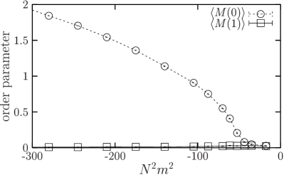
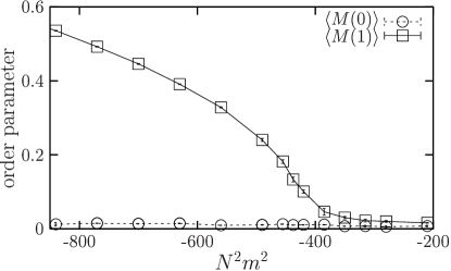
Figure 1: The momentum dependent order parameter $\langle M(k)\rangle$ (at $k=0,\,1$) against $N^{2}m^{2}$ at $N=35$. On the left we fixed $N^{2}\lambda=70$, which leads to the uniform phase. On the right we set $N^{2}\lambda=350$, so that a strongly negative $m^{2}$ leads to the striped phase.

As an example, figure 1 shows the results for $\langle M(0)\rangle$ and $\langle M(1)\rangle$ at $N=T=35$ and small $\lambda$ (on the left) resp. large $\lambda$ (on the right). As $m^{2}$ decreases, the uniform resp. staggered order is observed to set in unambiguously.

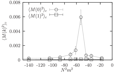
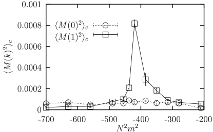
Figure 2: The connected two-point function of the momentum dependent order parameter, $\langle M(k)^{2}\rangle_{c}$ against $N^{2}m^{2}$ at $N=35$ and $N^{2}\lambda=70$ (on the left) resp. $N^{2}\lambda=350$ (on the right). We observe marked peaks, which allow us to localize well the phase transitions that we saw before in figure 1.

However, from such plots the critical value of $m^{2}$ can only be read off approximately. For a more precise localization of the disorder-order phase transition we measured the connected two-point function $\langle M(k)^{2}\rangle_{c}$, which has a peak at the phase transition (for $N\to\infty$ it diverges at this point). In figure 2 we show the results for the phase transitions illustrated before in figure 1. Indeed we find marked peaks which allow for an accurate determination of the transition from the disordered phase to the uniformly ordered phase (on the left) or — at larger $\lambda$ — to a striped phase (on the right).

(a) $N^{2}\lambda=90,~{}N^{2}m^{2}=-22.5$

(b) $N^{2}\lambda=900,~{}N^{2}m^{2}=-360$

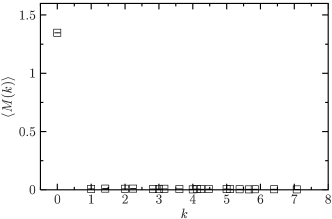
(c) $N^{2}\lambda=90,~{}N^{2}m^{2}=-225$

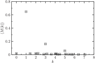
(d) $N^{2}\lambda=900,~{}N^{2}m^{2}=-1350$

Figure 3: The order parameter $\langle M(k)\rangle$ at different momenta $k$, at $N=T=45$.

In figure 3 we take a look at $\langle M(k)\rangle$ at the (discrete) values of $k$ in the range $k=0\dots 7$. As long as $m^{2}$ is not strongly negative, no order can be found at any frequency, so we are manifestly in the disordered phase (plots on top). Moving on to $m^{2}\ll 0$ we find at small $\lambda$ clearly the uniform order, since only $\langle M(0)\rangle$ deviates from zero (plot below on the left). Finally at larger $\lambda$ the Ising order parameter $\langle M(0)\rangle$ drops to zero again, and we observe a clear signal at $k=1$, i.e. a two-stripe pattern (plot below on the right). In this case, we also see some signals at $k=3$ and $5$. However, this should not be interpreted as an indication of an underlying multi-stripe structure. What happens is that only close to the phase transition the two stripes approximate a sine shape; for even lower $m^{2}$ they approximate more and more a step shape, and what we see here is simply the Fourier decomposition of such a pattern. This transition is illustrated in figure 4.

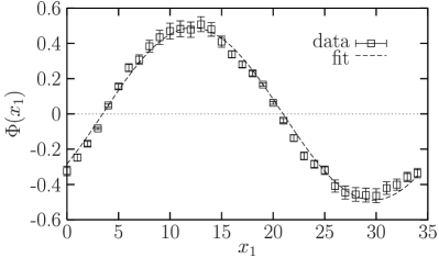
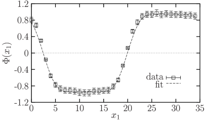
Figure 4: The profile $\Phi(x_{1})=\frac{1}{NT}\sum_{x_{2},t}\phi(x)$ of a simple two-stripe pattern at $N=35$, $N^{2}\lambda=350$: near the disordered phase a sine shape dominates (on the left, $N^{2}m^{2}=-250$), but at even lower $m^{2}$ the profile approximates a step shape (on the right, $N^{2}m^{2}=-620$). (These two plots are based on single configurations, and the error bars refer to the sum in $\Phi(x_{1})$.)

A really stable multi-stripe pattern is hard to find — as we will discuss later — and in that case we should see $\langle M(k\leq\sqrt{2})\rangle\simeq 0$ and find a signal only at higher $k$.

4 The phase diagram

In the previous section we explained our tools to explore the phase diagram. In particular, decreasing $m^{2}$ at fixed $\lambda$ we could localize the disorder-order phase transition accurately, and determine the type of order that emerged.

The next step is to repeat this procedure at various values of $N=T$ and search for suitable axes so that the phase diagram stabilizes for increasing $N$. The result is shown in figure 5. We obtained an explicit phase diagram with the qualitative features conjectured by Gubser and Sondhi.

It turns out that the axes $N^{2}m^{2}$ and $N^{2}\lambda$ are suitable for a large $N$ extrapolation. The power of $N$ multiplying the self-coupling is singled out by the transition inside the ordered regime between the uniform and striped phase. That phase transition, however, cannot be localized to the same precision as the disorder-order transition. The reason for this property will be clarified later on in the discussion of the dispersion relation (section 6). Still the stabilization of this region in $N$ is ultimately compelling.

Of course, the question about the order of the phase transitions is of interest, but (as in many other models) it is difficult to arrive at an absolutely safe answer. To get insight into this question, we searched for a hysteresis behavior by crossing the phase transition lines. If we cross the transition between disorder and order, we do not see any hysteresis effect. We have checked this behavior to a high precision for the transition from the disordered phase to both, the uniform and the striped phase, see figure 6. Hence we assume that transition to be of second order.

The situation with respect to the uniform-striped transition is unclear: for increasing $\lambda$ in the ordered regime, stripes do eventually show up. On the other hand, for decreasing $\lambda$ it seems to be hardly possible to make the stripes disappear again. This behavior is illustrated in figure 6.

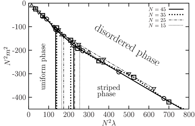
Figure 5: The phase diagram of the 3d $\lambda\phi^{4}$ model with two NC coordinates, identified from (indirect) lattice simulations with lattice size $N^{3}$.

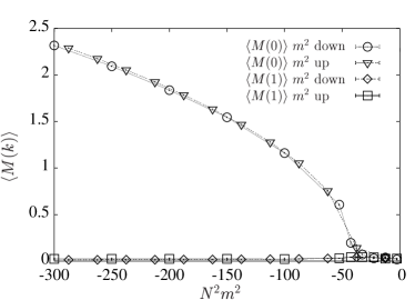
(a) $N^{2}\lambda=50$

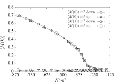
(b) $N^{2}\lambda=500$

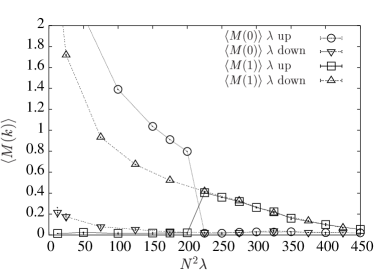
(c) $N^{2}m^{2}=-250$

Figure 6: An illustration of the hysteresis behavior described in the text: for the disorder-order phase transition, no hysteresis can be observed, as we show for the case that the uniform resp. striped order is involved (above, on the left resp. on the right). Below we show the outcome for the uniform-striped transformation: once a stripe pattern is built, a return to the uniform order is hardly possible inside the ordered regime, hence the “thermal cycle” does not close.

It is instructive to visualize typical configurations in the different phases. This can be achieved by mapping back the matrix configurations to the lattice. The mapping and inverse mapping between lattice configurations and matrices are briefly described in appendix A. For further details we refer to ref. [26]. Typical snapshots at low and at high values of $\lambda$ and of $-m^{2}$ are shown in figure 7.

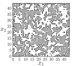
(a) $N^{2}\lambda=70,~{}N^{2}m^{2}=-17.5$

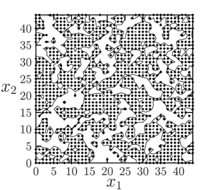
(b) $N^{2}\lambda=700,~{}N^{2}m^{2}=-350$

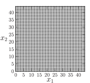
(c) $N^{2}\lambda=70,~{}N^{2}m^{2}=-280$

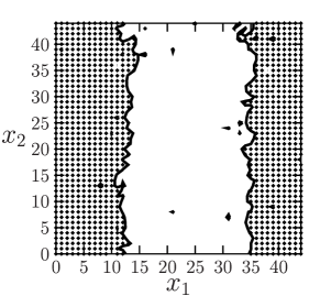
(d) $N^{2}\lambda=700,~{}N^{2}m^{2}=-910$

Figure 7: Typical lattice configurations at $N=T=45$ for low $-m^{2}$ (on top) and high $-m^{2}$ (below), and for weak $\lambda$ (on the left) and strong $\lambda$ (on the right). The dotted and blank area represent the domains with different signs of $\phi(x)$. We recognize disorder in both cases on top, and a uniform resp. striped order below.

In particular we clearly see a two stripe pattern in the plot on bottom on the right. The search for such obvious pictures also for multi-stripe and checkerboard patterns — which are safely stable in the Monte Carlo history — turned out be very difficult. Quite clear hints for such patterns can be seen at relatively large $N$ and a strong self-coupling $\lambda$; examples are shown in figure 8.

However, if we just map the configurations back to the lattice and illustrate it as in figures 7 and 8, the emerging pictures do not show a convincing dominance of one stable multi-stripe pattern, unlike the case of two stripes parallel to one axis at lower $\lambda$.

(a) $N=35$, $\lambda=10$, $m^{2}=-4$

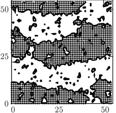
(b) $N=55$, $\lambda=50$, $m^{2}=-22$

Figure 8: Examples for a pattern with two diagonal stripes (on the left) and of four stripes parallel to an axis (on the right). They were observed in the histories at $N=35$, $\lambda=10$, $m^{2}=-4$, resp. $N=55$, $\lambda=50$, $m^{2}=-22$. However, it is difficult to verify the ultimate stability of such non-minimal stripe patterns.

If we really want to confirm the Gubser-Sondhi conjecture we need evidence that in the limit, which corresponds to the continuum and to infinite volume, a finite stripe width dominates. Hence in this limit we expect an infinite number of stripes in various directions, with a finite width. Since it is very difficult to find evidence for this behavior by a direct illustration, we will search for it in a more subtle manner in sections 6 and 7. That investigation is based on correlation functions, so this is what we want to discuss next.

5 Correlation functions

We first take a look at the spatial correlation function

$$C(\vec{x})=\frac{1}{N^{2}T}\sum_{\vec{y},t}\langle\phi(\vec{x}+\vec{y},t)\phi(\vec{y},t)\rangle\,.$$ (24)

As an example we plot in figure 9 the correlators $C(x_{1},0)$ and $C(0,x_{2})$ at $N=T=45$ in the four sectors of the phase diagram, which we also distinguished in figure 7. In all the sectors we confirm the expected behavior: a fast decay in both directions in the disordered phase, but hardly any decay in the uniform phase. In the case of two stripes (parallel to an axis), we observe a ferromagnetic behavior parallel to the stripes and an anti-ferromagnetic behavior vertical to them.

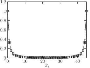
(a) $N^{2}\lambda=90,~{}N^{2}m^{2}=-22.5$

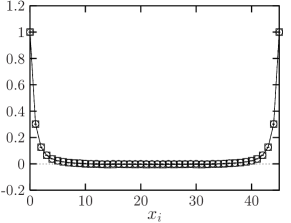
(b) $N^{2}\lambda=900,~{}N^{2}m^{2}=-360$

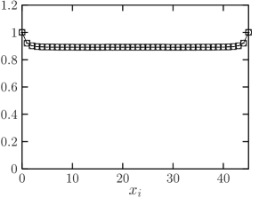
(c) $N^{2}\lambda=90,~{}N^{2}m^{2}=-225$

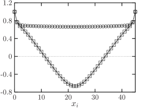
(d) $N^{2}\lambda=900,~{}N^{2}m^{2}=-945$

Figure 9: The spatial correlation function $C(\vec{x})$, defined in eq. (24) (with one component of $\vec{x}$ being $0$) in the different sectors of the phase diagram in figure 5, at $N=T=45$. In the disordered phase (the two plots above) we see a fast decay in both directions, both, for small and for large $\lambda$. In the uniform phase (below, left) there is hardly any decay, and in the case of two stripes (below, right) we observe a mixed ferromagnetic and anti-ferromagnetic behavior in the two directions.

Next we turn our interest to the fast decay in the disordered phase, at some point close to the ordering phase transition. Figure 10 shows logarithmic plots for these correlators, one close to the uniform phase (on the left) and the other one close to the striped phase (on the right). We see that the decay is somehow irregular: it is faster than polynomial, but it does not follow an exponential either. Of course the exponential decay is standard in the commutative world, so here we see that this property is distorted by the non-commutativity.

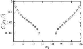
(a) $N^{2}\lambda=70,~{}N^{2}m^{2}=-17.5$

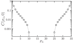
(b) $N^{2}\lambda=350,~{}N^{2}m^{2}=-140$

Figure 10: The spatial correlator in the disordered phase, close to the transition to the uniform phase (on the left) resp. to the striped phase (on the right). The logarithmic plots show that the decay is fast, but it does not follow an exponential.

Now we turn our attention to another type of correlation function, namely to the quantity

$$G(\tau):=\frac{1}{T}\sum_{t}\langle\tilde{\phi}(\vec{p}=\vec{0},t)^{*}\tilde{\phi}(\vec{p}=\vec{0},t+\tau)\rangle\,.$$ (25)

This function measures the correlation between two averaged spatial layers with a temporal separation of $\tau$. We denote $G(\tau)$ as the temporal correlator, but we should stress that the difference from the spatial correlator is not only that we deal with a separation in time.

In figure 11 we show typical examples also for this correlator in the four sectors of the phase diagram, in analogy to figure 9. Here we show directly logarithmic plots, which illustrate that this decay does follow an exponential — resp. a $\cosh$ function, i.e. an exponential with periodic boundary conditions — in the disordered phase and in the striped phase. In the uniform phase we obtain $G(\tau)\simeq 1$ for all values of $\tau$.

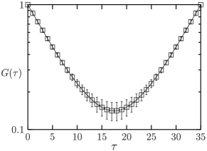
(a) $N^{2}\lambda=70,~{}N^{2}m^{2}=-35$

(b) $N^{2}\lambda=525,~{}N^{2}m^{2}=-140$

(c) $N^{2}\lambda=70,~{}N^{2}m^{2}=-140$

(d) $N^{2}\lambda=525,~{}N^{2}m^{2}=-560$

Figure 11: The temporal correlator $G(\tau)$, defined in eq. (25), in the different sectors of the phase diagram in figure 5, at $N=T=35$. We see a fast decay, which now follows well an exponential (resp.  a $\cosh$ shape) in the disordered phase (two plots above) and in the striped phase (below, right), whereas $G(\tau)$ is nearly constant in the uniform phase (below, left).

From the exponential decay in the disordered phase close to ordering we can now extract the energy at momentum $\vec{p}=\vec{0}$, i.e. the rest energy $E_{0}$. We evaluate this quantity at some time separation $\tau$ as

$$E_{0}=-\ln\frac{G(\tau+1)}{G(\tau)}\,.$$ (26)

Such a term is sensible if this evaluation yields a plateau over some range of $\tau$, which is not very close to the boundary nor to the center $T/2$, so that the exponential decay dominates. Figure 12 shows an example of the corresponding decay and for the neat plateau that one obtains for $E_{0}$ according to eq. (26).

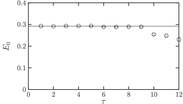
Figure 12: On the left: the temporal correlator $G(\tau)$ in the disordered phase, close to the transition to the striped phase (at $N=T=35$, $N^{2}\lambda=350$, $N^{2}m^{2}=-140$). For comparison, the line represents a cosh function. From the decay we extract the rest energy $E_{0}$ at different values of $\tau$, according to eq. (26). The plot on the right shows that this provides a stable plateau, up to the region around $T/2$ where the finite $T$ effects are significant.

The same procedure to extract the effective energy from an exponential decay can be repeated also for finite momenta $\vec{p}$. This leads to the full dispersion relation, which is the subject of the next section 6. For more general aspects of dispersion relations in NC field theory we refer to ref. [32].

6 The dispersion relation

We now generalize the correlation function $G(\tau)$ of eq. (25) and study the decay of the expectation value

$$\frac{1}{T}\sum_{t}\langle\tilde{\phi}(\vec{p},t)^{*}\tilde{\phi}(\vec{p},t+\tau)\rangle$$ (27)

at various momenta $\vec{p}$. In the disordered phase close to the ordering transition we always find an exponential decay in $\tau$, which allows us to extract the energy $E(\vec{p})$. In figure 13 we show the resulting dispersion relation at $N=T=35$ for a small, a moderate and a large value of $\lambda$. In the first case — near the uniform phase — $E^{2}(\vec{p}^{\,2})$ follows closely the usual linear form, which confirms again that at small $\lambda$ this model looks like its commutative counterpart.

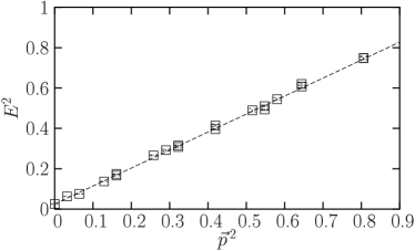
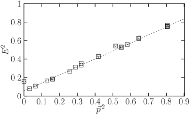
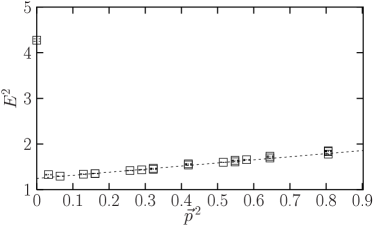
Figure 13: The dispersion relations measured at $N=35$ in the disordered phase, close to the ordering transition. We proceed from small $\lambda$ (on top: $\lambda=0.06$, $m^{2}=-0.01$) to moderate $\lambda$ (on the left: $\lambda=0.6$, $m^{2}=-0.23$) and finally to large $\lambda$ (on the right: $\lambda=100$, $m^{2}=-7$). In the first case, which is close to the uniform phase, we see the standard linear dispersion relation. As $\lambda$ increases we are close to the striped phase, and the energy minimum moves to a finite momentum $|\vec{p}|$. The location of the minimum and the rest energy grow for raising values of $\lambda$.

As $\lambda$ increases we see an amplified rest energy (at $\vec{p}=\vec{0}$), followed by a sharp dip at low momenta and again the linear curve asymptotically at larger momenta. Of course, the observation $E_{0}>0$ agrees with the UV/IR mixing. Our result confirms that this mixing also occurs non-perturbatively, as we announced in section 1. The question of an IR divergence, i.e. a divergence of $E_{0}$ in the double scaling limit of zero lattice spacing and infinite volume, will be addressed in the next section.

The fact that the energy minimum drives to finite momenta is the basis for the striped phase that we illustrated before in section 4. If such momenta condense they manifest themselves in the stabilization of some stripe patterns. For instance, in the second plot of figure 13 (at $\lambda=0.6$) the leading non-zero momentum which occurs in this volume is clearly the location of the energy minimum. This momentum corresponds to $k=1$ in the notation of eq. (23), hence in this case a condensation of the mode with minimal energy leads to two stripes parallel to one of the axes.

In the last example in figure 13 there are several non-zero momenta which are close to the minimum. In such situations various types of stripe patterns may condense. The transition between them does not come about easily, so they all appear stable even if they do not correspond to the exact minimum. In such cases we could see multi-stripe patterns as in figure 8, but it was difficult to figure out which pattern is ultimately most stable. The dispersion relation now clarifies the situation as a coexistence of qualitatively different, practically stable patterns in the vicinity of the energy minimum. If we start from such a point in the disordered phase and lower $m^{2}$, the configuration takes one of the stripe patterns which correspond to the $k$ values near the minimum. Once this pattern is built up, it is hardly possible to change it again as long as we are in the ordered regime (obviously this would require a large deformation in the structure of the configuration). For the same reason the transition between the uniform and the striped phase could not be determined accurately based on a direct illustration, as we described in section 4. However, it is the very nature of the system that such transitions happen gradually over a broad interval in $\lambda$.

As a further example, we show a dispersion relation for $N=T=55$ in figure 14. Here we have a finer resolution of the momenta. Now the momentum that corresponds to $k=1$ is clearly not the minimum any more, but the minimal vicinity involves the cases $k=\sqrt{2}$, $2$ and $\sqrt{5}$. From the phase diagram in figure 5 it is clear that for the given parameters $m^{2}=-15$, $\lambda=50$ we are near the striped phase, so here we have at last an evidence for the existence of stable multi-stripe patterns.

Figure 14: The dispersion relation determined at $N=55$, $m^{2}=-15$, $\lambda=50$. The symbols correspond to the discrete values of $k=N|\vec{p}|/(2\pi)$ that occur, i.e. $k=1$, $\sqrt{2}$, $2$, $\sqrt{5}$, $\sqrt{8}$, $\dots$

The dispersion relation observed in figure 14 can be parameterized to a good accuracy as

$$E^{2}(\vec{p}^{\,2}) = c_{0}\,\vec{p}^{\,2}+m^{2}+\frac{c_{1}}{\sqrt{\vec{p}^{\,2}+\bar{m}^{2}}}\exp\left(-c_{2}\sqrt{\vec{p}^{\,2}+\bar{m}^{2}}\right)$$

$$\hbox{with}\quad c_{0} = 0.919(4)\,,\quad c_{1}=0.07(1)\,,\quad c_{2}=13(1)\,,\quad\bar{m}^{2}=0.0004(1)\,,$$ (28)

which is illustrated by the curve in figure 14. (We assume the slight deviation of $c_{0}$ from its expected value $1$ to be a finite $N$ artifact.) The square root in this formula is characteristic for the three dimensional case, and an obvious ansatz for a linear IR divergence in $E^{2}$ (regularized by the term $\bar{m}^{2}$ and suppressed at larger $\vec{p}^{\,2}$). We remark that in $d=4$ one would expect the corresponding formula with the square root replaced both times by $(\vec{p}^{\,2}+\bar{m}^{2})$. In $d=3$ and $4$ this form can be related to $\Gamma^{(1)}_{\rm np}$ given in eq. (11) [26]. In our 3d results the fits work in fact much better with eq. (28) than with the expected 4d formula.

7 The continuum limit

In order to study the extrapolation of our results to a continuous, non-commutative space, we first have to identify a dimensionful lattice spacing. We perform this identification in the planar limit, where one sends $N\to\infty$ at fixed parameters $m^{2}$ and $\lambda$.

We saw in section 6 that the dispersion relation $E^{2}(\vec{p}^{\,2})$ becomes linear for relatively large momenta. In figure 15 we study this behavior in the planar limit: we see that the linear regime is not altered any more as we approach this limit, and that the dip for the minimum is squeezed towards zero momentum. This implies that the behavior at relatively large momenta is dominated by the planar contribution. Hence we can extrapolate a dispersion relation to the planar limit by just extending the linear slope down to $\vec{p}^{\,2}=0$.

This is analogous to our study of the 2d NC $\mathop{\rm{}U}\nolimits(1)$ gauge theory, where we saw an area law for Wilson loops at a small area [16]. Thus it coincided with the analytic result by Gross and Witten for (commutative) $\mathop{\rm{}U}\nolimits(N)$ Yang-Mills theory in the planar limit [33].

Figure 15: The dispersion relation (at $\lambda=50$, $m^{2}=-13.2$) as we approach the planar limit. The linear regime is stable, and the minimum moves close to $0$.

Making use of this property, we determine an effective mass $M_{\rm eff}$ in the planar limit. We only consider the “linear dispersion regime” where the momentum $|\vec{p}|$ is large enough to follow the linear dispersion behavior

$$E^{2}\simeq M_{\rm eff}^{2}+\vec{p}^{\,2}\,.$$ (29)

If the momenta are not too small, this relation is fulfilled to a high precision — as we saw from figures 13 and 14 — hence we can evaluate an accurate value for $M_{\rm eff}^{2}$ in lattice units. In particular, we fixed again $\lambda=50$ and considered various values of $m^{2}$; in each case we searched for the planar limit, i.e. a stabilization of the resulting effective mass as $N$ increases.

Figure 16: The effective mass squared as a function of the bare mass squared in the disordered phase. We observe a linear behavior, which stabilizes accurately in the planar large $N$ limit.

This is indeed the case in the range $N=15\dots 45$. Figure 16 shows that the results for $M^{2}_{\rm eff}$ depend linearly on $m^{2}$, as long as we are in the disordered phase. We parameterize this linear curve as

$$M^{2}_{\rm eff}=\mu^{2}+\gamma\,m^{2}\,,$$ (30)

and we show in figure 17 that the values we obtain for $\mu^{2}$ and $\gamma$ are stable in $N$.

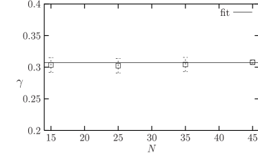
Figure 17: The terms $\mu^{2}$ and $\gamma$ in the parameterization (30), at $\lambda=50$. They are found to be constant in $N$ to a good approximation.

Our condition for the continuum limit is now that we keep the effective mass in physical units, $M_{\rm eff}/a$, constant in the planar limit, where $a$ is the lattice spacing. Without loss of generality we simply set $M_{\rm eff}/a=1$, which means that we measure every quantity which has the dimension of a length in units of $\,a/M_{\rm eff}$. This corresponds to identifying the lattice spacing as

$$a^{2}=\mu^{2}+\gamma\,m^{2}\,.$$ (31)

The ratio $m_{c}^{2}=-\mu^{2}/\gamma$ represents the squared critical bare mass, and according to our result illustrated in figure 17 we obtain

$$m_{c}^{2}=-15.01(8)\,,$$ (32)

which is of course also in agreement with figure 16.

Therefore, in the double scaling limit — which keeps the non-commutativity parameter $\vartheta$ in eq. (7) constant — we have to fix $N(\mu^{2}+\gamma\,m^{2})$, while taking the limits $N\to\infty$ and $m^{2}\to m_{c}^{2}$. This limit involves a free constant, which fixes the value of the non-commutativity parameter $\vartheta$. We choose it as

$$Na^{2}=100\gamma\quad\Rightarrow N(m^{2}-m_{c}^{2})=100\,,$$ (33)

$$\vartheta=\frac{100\gamma}{\pi}=9.77(6)\,.$$

The value for $N(m^{2}-m_{c}^{2})$ is taken rather large, so that we do not get too close to the critical mass for the $N$ values that we are using (otherwise we would risk numerical problems due to large fluctuations).

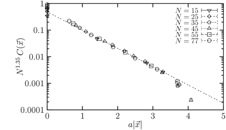
Figure 18: The spatial correlator $C(\vec{x})$ defined in eq. (24), amplified by a wave function renormalization factor $N^{1.35}$, against the physical distance $a|\vec{x}|$. We see a double scaling regime, which corresponds to the non-commutative continuum limit. (The dashed line marks the linear regime of this double scaling limit.)

In this framework, we first measure the spatial correlator, which was defined before in eq. (24). A double scaling behavior can be observed if the spatial correlator is multiplied by a wave function renormalization factor $N^{\alpha}$, where the suitable power is found to be $\alpha=1.35$. Then a scaling region shows up, as figure 18 shows.

Finally we are equipped to approach the question, which represents the real challenge in this context: we now want to verify if the striped phase persists in the continuum limit.

To this end, we consider the double scaling limit of the dispersion relation. The crucial question is whether or not the dispersion minimum stabilizes at a finite momentum. If such a minimum survives the double scaling limit, it indicates the existence of a striped phase in the continuum, where the value of the minimal momentum characterizes the dominating stripe width in the infinite, non-commutative space.

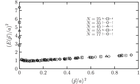
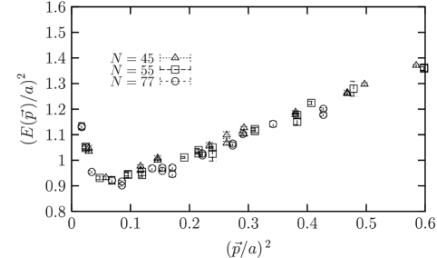
Figure 19: The dispersion relation at $\lambda=50$ and $\vartheta\simeq 9.77$ (in physical units), with energy and momentum expressed in physical units. We see the linear regime starting at moderate momenta, a minimum around $(\vec{p}/a)^{2}\mathop{\lesssim}0.1$, and a rest energy $E_{0}$, which increases rapidly with $N$, see also figure 20. The plot on top provides an overview, and below we zoom the region around the minimum. This result confirms that the dispersion relation stabilizes in the double scaling limit to the continuum and infinite volume, which corresponds to large $N$ in this figure.

The plots in figures 19 demonstrate that at finite momentum the dispersion relation does indeed stabilize in the double scaling limit. For $N=25\dots 77$, a universal minimum is found around $(\vec{p}/a)^{2}_{\rm min}\mathop{\lesssim}0.1$. Of course, this number refers to the specific values of $\vartheta$ and $\lambda$ that we have chosen. We recall that here we are working in the disordered phase, which also holds for figure 19. It would be very difficult to extrapolate to the double scaling limit inside the striped phase, because there the finite $N$ boundary conditions have a very strong impact. Hence our strategy is to work in the disordered phase (where the finite $N$ effects are rather harmless, as figures 9 and 10 show) close to the striped phase, and extract from there information about the striped phase in the continuum, by identifying the modes that will condense at lower $m^{2}$.

In particular this result shows that the model is non-perturbatively renormalizable. In fact the way we identified the lattice spacing amounts to choosing it in such a way that the high momentum region of the dispersion relation scales in the double scaling limit. What is really non-trivial, therefore, is that the large $N$ scaling extends to the low momentum region, where it deviates from the planar linear behavior observed at higher momenta. This corresponds to the continuum limit of the non-commutative field theory at finite $\vartheta$.

We remark that in this model also the renormalizability of the perturbative series may seem less problematic than in other cases, since the commutative $\lambda\phi^{4}$ model is super-renormalizable. However, to the best of our knowledge the perturbative renormalizability of the 3d NC $\lambda\phi^{4}$ model has not been shown in the literature.

At last we take a look at the double scaling of the rest energy $E_{0}$. Figure 20 shows that it diverges linearly in $\sqrt{N}\propto 1/a$. Therefore we do find an IR divergence in the continuum limit, in full agreement with the concept of UV/IR mixing — we recall that also the UV divergence in this model is linear, as eq. (11) shows. This IR divergence confirms that the non-planar terms survive the continuum limit that we take by the double scaling described here, and they strongly affect the continuum behavior.

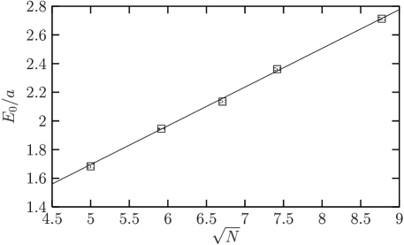
Figure 20: The rest energy in physical units as a function of $\sqrt{N}\propto 1/a$. We clearly recognize a linear IR divergence in the continuum limit.

8 A Nambu-Goldstone mode in the striped phase

In the striped phase the translational symmetry is spontaneously broken. According to the Goldstone Theorem, we expect the emergence of a zero-energy mode in the continuum theory. Generalities about Nambu-Goldstone (NG) bosons in NC field theory are discussed in refs. [34].

On the lattice the NG mode acquires a small energy since the translational symmetry is discretized. In this section we present numerical results from the striped phase on this issue.

When dealing with the spontaneous breakdown of a symmetry, one has to define the vacuum expectation values (VEVs) with some care to make them meaningful. In figure 9 (below, right), for instance, we have rotated each configuration before the measurements so that the stripe pattern is oriented in one particular direction. More precisely we have rotated each configuration such that the momentum $\vec{p}$ which gives the maximum in $M(k)$ — defined in eq. (23) — points to a particular direction.

The standard VEV $\langle\phi(\vec{x},t)\rangle$ vanishes all over the phase diagram. Alternatively we now introduce an oriented VEV, which is based on configurations which are all rotated and shifted before the measurements. In this section we restrict our attention to the two-stripe patterns parallel to an axis. We define the oriented VEV by a rotation so that the stripes are vertical to the $x_{2}$-axis, and in addition by shifts on the rotated configurations,

$$\phi^{\prime}(\vec{x},t)=\phi(x_{1},x_{2}-\sigma,t)_{\rm rotated}\,,$$ (34)

which maximize the overlap with a characteristic profile.

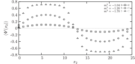
Figure 21: The oriented VEV $\langle\Phi^{\prime}(x_{2})\rangle=\frac{1}{NT}\sum_{x_{1},t}\langle\phi^{\prime}(\vec{x},t)\rangle$ against $x_{2}$ for $\lambda=2$ and $m^{2}=-1.04,-1.2,-1.7$. Rotations and shifts are carried out before taking the ensemble average, as we described in the text.

For simplicity we use the step profile ${\rm sign}(N/2-x_{2})$, so we determine the shift $\sigma$ by maximizing the overlap $\sum_{\vec{x},t}\phi^{\prime}(\vec{x},t)\,{\rm sign}(N/2-x_{2})$. In figure 21 we show the results for the oriented VEV

$$\langle\Phi^{\prime}(x_{2})\rangle=\frac{1}{NT}\sum_{x_{1},t}\langle\phi^{\prime}(\vec{x},t)\rangle\,.$$ (35)

The feature is very similar to figure 4 (where we considered single configurations), and it demonstrates that the translational symmetry in the $x_{2}$-direction is broken spontaneously.

Performing a Fourier transformation, we find that $\frac{1}{NT}\sum_{t}\langle\tilde{\phi}(\vec{p},t)\rangle$ is non-zero for $\vec{p}=(0,\frac{2\pi}{N})$. Deeper in the striped phase we also have condensations for $\vec{p}=(0,\frac{2\pi}{N}n_{2})$ with $n_{2}=3,5,\dots$, which corresponds to the deformation of the leading sine pattern as we have seen in figure 3. Note that the pattern is characterized by anti-periodicity in the $x_{2}$-direction with the period $N/2$, and a constant behavior in the $x_{1}$-direction. All the modes consistent with this periodicity may condense. Due to the condensation of non-zero momentum modes, the momentum is no longer conserved in the striped phase.

In the continuum we can identify the NG mode in the standard manner. We introduce a field $\phi^{\prime}(x,t)$ in analogy to eq. (34), i.e. oriented such that the dominant stripes are vertical to the $x_{2}$ axis, and shifted properly. Let us then decompose this field $\phi^{\prime}(x,t)$ into the VEV and the fluctuation as

$$\phi^{\prime}(\vec{x},t)=\langle\phi^{\prime}(\vec{x},t)\rangle+\delta\phi^{\prime}(\vec{x},t)\,.$$ (36)

In the case of the assumed stripe pattern, the VEV is not invariant under the shift in the $x_{2}$ direction. The corresponding NG mode is given by the infinitesimal translation in the $x_{2}$ direction as

$$\delta\phi^{\prime}(\vec{x},t)\propto\frac{\partial}{\partial x_{2}}\langle\phi^{\prime}(\vec{x},t)\rangle\,.$$ (37)

Thus we find that the NG mode has the same Fourier components as the VEV $\langle\phi^{\prime}(\vec{x},t)\rangle$ itself.

In order to reveal the existence of the NG mode, we repeat the analysis which we performed before to study the dispersion relation in the disordered phase. Let us define the connected two-point function

$$G(\vec{p},\vec{q};\tau)_{c}:=\frac{1}{N^{2}}\left[\frac{1}{T}\sum_{t}\langle\tilde{\phi}^{\prime}(\vec{p},t)^{*}\tilde{\phi}^{\prime}(\vec{q},t+\tau)\rangle-\left(\frac{1}{T}\sum_{t}\langle\tilde{\phi}^{\prime}(\vec{p},t)^{*}\rangle\right)\left(\frac{1}{T}\sum_{t}\langle\tilde{\phi}^{\prime}(\vec{q},t)\rangle\right)\right].$$ (38)

Unlike the behavior in the disordered phase, the two-point function can take non-zero values also for $\vec{p}\neq\vec{q}$ because of the non-conservation of the momentum. From the exponential decay with respect to $\tau$, we can extract the energy of the intermediate state which couples to the operators considered, as we have done in section 6 in the disordered phase. When the two-stripe pattern is formed, the subtraction of the disconnected part is needed for $\vec{p}=(0,\frac{2\pi}{N}n_{2}^{(p)})$ and $\vec{q}=(0,\frac{2\pi}{N}n_{2}^{(q)})$, where $n_{2}^{(p)}$ and $n_{2}^{(q)}$ are odd integers. It is precisely this case where the quasi NG mode is expected to appear.

In figure 22 we plot the energies extracted from the two-point function $G(\vec{p},\vec{p};\tau)_{c}$ for some low momentum modes against the bare mass squared. In order to see the $N$ dependence, we compare the results for $N=21$ and $N=25$.

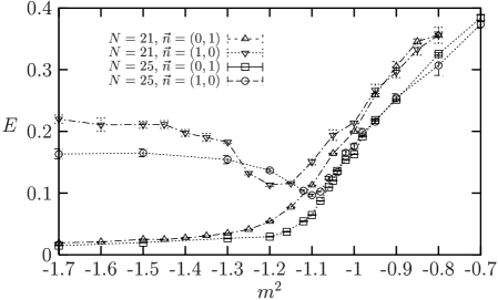
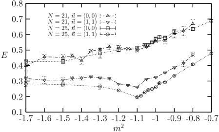
Figure 22: The energies extracted from the connected two-point function, against the bare mass squared for $N=21$ and $N=25$ at $\lambda=2$. We show above the results for the modes $(0,\frac{2\pi}{N})$ and $(\frac{2\pi}{N},0)$, and below the results for the modes $(0,0)$ and $(\frac{2\pi}{N},\frac{2\pi}{N})$ (with $\vec{p}=2\pi\vec{n}/N$).

The energy extracted from the $(\frac{2\pi}{N},0)$ mode and the $(0,\frac{2\pi}{N})$ mode coincide in the disordered phase, but they differ in the striped phase because the rotational invariance is broken. The energy of the $(\frac{2\pi}{N},0)$ mode and the $(\frac{2\pi}{N},\frac{2\pi}{N})$ mode have a minimum near the critical point. The minimum values decrease for larger $N$, and they seem to approach zero, having a cusp-like dip. Thus these modes are expected to have finite dimensionful energy in the continuum limit.

The energy of the $(0,\frac{2\pi}{N})$ mode is small in the striped phase, and it becomes even smaller as $N$ increases. At larger $N$ the energy seems to approach zero not only at the critical point, but all the way in the striped phase. This behavior suggests the existence of the quasi NG mode in the striped phase, whose tiny non-zero energy is due to the discretization of the translational symmetry. Our results also support that the discretization effects are governed by the ratio of the lattice spacing to the wave length of the stripe pattern, which goes to zero at large $N$ in the striped phase.

The energy extracted from the zero mode $(0,0)$ does not have a minimum near the critical point and it does not decrease as $N$ increases. This is consistent with our observation in the disordered phase that the dispersion relation has an infrared singularity, and the $(0,0)$ mode, in particular, has as energy which diverges linearly with the cutoff scale as shown in figure 20.

9 Conclusions

We have presented a comprehensive non-perturbative study of the $\lambda\phi^{4}$ model in a three dimensional space, with two non-commutative spatial coordinates and a commutative Euclidean time. The non-commutativity tensor is constant. This system is lattice discretized and then mapped onto a hermitean matrix model. This mapping is of great advantage for our numerical simulations, which would be extremely tedious to run directly on the lattice because of the star product.

We introduced a set of order parameters which are able to detect the uniform order as well as various types of stripe patterns. Measuring numerically the expectation values of these order parameters, we could explore the explicit phase diagram of the lattice discretized model, see figure 5. Its structure is consistent with an earlier qualitative conjecture by Gubser and Sondhi: at strongly negative $m^{2}$ some order emerges, which is uniform at small $\lambda$ (as in the commutative case), but which is dominated by stripe patterns at larger $\lambda$. The latter is unknown in the commutative $\lambda\phi^{4}$ model; we denoted it as the striped phase. The phase transition between the disordered phase and the ordered regime seems to be of second order, both, for the uniform order and for the striped order.

We then studied spatial correlation functions, which decay in an irregular way due to the non-commutative spatial geometry. On the other hand, the temporal correlation functions decay exponentially. That property allowed us to evaluate the dispersion relation of the scalar field, in particular in the disordered phase close to the ordering transition. In the vicinity of the uniform phase we find the usual linear dispersion, whereas the vicinity of the striped phase corresponds to the case of an energy minimum at a finite momentum. In fact, the stripe formation means a condensation of such modes of lower energy than the zero momentum mode.

If the momentum is not that small, we enter — also in the vicinity of stripes — into a linear regime of the dispersion relation. From the extrapolation of this linear behavior we obtained an effective mass, which allowed us to identify a “physical” (i.e. dimensionful) lattice spacing $a$ (in the planar limit). This provides a prescription how to take the limit to the NC $\lambda\phi^{4}$ model in the continuum: we take the double scaling limit, which keeps the product $Na^{2}$ constant, where $N$ is the size of the lattice resp. the matrices. Thus we fix the non-commutativity parameter $\vartheta$. Approaching this limit, which is at the same time an infinite volume limit, we found stable dispersion relations. In particular, the shift of the energy minimum to a finite momentum survives this limit, which shows that the striped phase is indeed there to stay in the continuum. This limit completes the confirmation of the conjecture by Gubser and Sondhi. Moreover, the convergence of the dispersion in the double scaling limit shows that this model can be renormalized non-perturbatively.

The stripe formation implies the spontaneous breaking of translation and rotation invariance in the spatial plane. The Nambu-Goldstone mode of the broken translation symmetry can be seen approximately from the numerical data. Interestingly, this symmetry breaking also occurs in the two dimensional model, see ref. [27] and appendix B. This is possible because this model does not obey the assumptions for the proof of the Mermin-Wagner Theorem.

The energy of the zero mode itself (rest energy) diverges in the limit of zero lattice spacing and infinite volume. This confirms that the UV/IR mixing is a fundamental property of NC field theories, which is also manifest beyond perturbation theory. Diagrammatically, this mixing effect is driven by the non-planar diagrams, which are not suppressed in the double scaling limit (in contrast to the planar limit). This mixing is the basis for the different types of long ranged orders that occur in this model.

As an outlook, we are now elaborating a dispersion relation for the photon (or, strictly speaking, for the corresponding “glueball”) in a four dimensional NC space [35]. We have studied earlier QED in a NC plane [16], where we already saw striking manifestations of UV/IR mixing. We expect such effects also in four dimensions, in particular a $\Theta$-deformed dispersion relation for the photon. This dispersion has been studied before to one loop in perturbation theory [36], though with an uncontrolled behavior of higher orders. In contrast, explicit non-perturbative results would allow us to establish bounds on the magnitude of the non-commutativity in nature.

For instance, blazars (highly active galactic nuclei) are assumed to emit bursts of photons simultaneously, which cover a broad range of energies, see e.g. ref. [37]. Experimentalists are already trying to detect a relative delay of these photons upon their arrival on earth, depending on the frequency [38]. Such experimental efforts will be intensified in the near future. For instance, the GLAST project [39] is scheduled to be launched in 2006 and to monitor gamma rays from $20\,{\rm MeV}$ up to $1\,{\rm TeV}$. If we arrive at results for the $\Theta$-deformed photon dispersion — analogous to figure 19 — they could then be confronted with such experimental data [40].

Appendix A The mapping between the lattice and the matrix formulation

To describe the connection between the lattice formulation and the matrix model that we actually simulated, we first go back to the continuum and introduce the terminology of Weyl operators.

We start from a scalar field $\phi(x)$ in the (commutative) euclidean space $\mathbb{R}^{d}$, which falls off fast enough for the Fourier integral

$$\tilde{\phi}(p)=\int d^{d}x\,\phi(x)e^{-ix_{\mu}p_{\mu}}$$ (39)

to converge. The corresponding NC space is characterized by the coordinate operators $\hat{x}_{\mu}$, which obey the non-commutativity relation (1). We recall that we are dealing with commutative momenta in the NC space. Now we introduce the Weyl operators

$$\hat{W}[\phi]=\frac{1}{(2\pi)^{d}}\int d^{d}p\,\tilde{\phi}(p)\ e^{i\hat{x}_{\mu}p_{\mu}}\,,$$ (40)

which build a NC, associative algebra. In coordinate space, the map between the scalar fields and the corresponding Weyl operators reads

$$\hat{W}[\phi]=\int d^{d}x\,\phi(x)\hat{\Delta}(x)\,,\qquad\hat{\Delta}(x)=\frac{1}{(2\pi)^{d}}\int d^{d}p\,e^{i(\hat{x}_{\mu}-x_{\mu})p_{\mu}}\,,$$ (41)

where $\hat{\Delta}(x)$ is a hermitean operator.

Derivatives of the Weyl operators are defined by an anti-hermitean operator $\hat{\partial}_{\mu}$, which obeys

$$[\hat{\partial}_{\mu},\hat{x}_{\nu}]=\delta_{\mu\nu}\quad\rightarrow\quad[\hat{\partial}_{\mu},\hat{\Delta}(x)]=-\partial_{\mu}\hat{\Delta}(x)\,.$$ (42)

This implies the desired property

$$[\hat{\partial}_{\mu},\hat{W}[\phi]\,]=\hat{W}[\partial_{\mu}\phi]\,.$$ (43)

Hence a translation can be expressed by unitary operators $\exp(v_{\mu}\hat{\partial}_{\mu})$, (c.f. eqs. (19) and (20)),

$$\hat{\Delta}(x+v)=e^{v_{\mu}\hat{\partial}_{\mu}}\hat{\Delta}(x)e^{-v_{\mu}\hat{\partial}_{\mu}}\,.$$ (44)

Accordingly a trace on the algebra of Weyl operators is translation invariant, and it is given explicitly by

$$\mathop{\rm Tr}\nolimits\,\hat{W}[\phi]=\int d^{d}x\,\phi(x)\,,\quad\mathop{\rm Tr}\nolimits\,\hat{\Delta}(x)=1\,.$$ (45)

If $\Theta$ is invertible — which requires the dimension $d$ of the NC space to be even — it can be shown that [12]

$$\mathop{\rm Tr}\nolimits\left(\hat{\Delta}(x)\hat{\Delta}(y)\right)=\delta^{(d)}(x-y)\,.$$ (46)

Thus we arrive at the inverse map

$$\phi(x)=\mathop{\rm Tr}\nolimits\left(\hat{W}[\phi]\,\hat{\Delta}(x)\right).$$ (47)

Based on this inverse map, we obtain the product of Weyl operators as

$$\hat{W}[\phi]\,\hat{W}[\psi]=\hat{W}[\phi\star\psi]\,,$$ (48)

which justifies the use of the star product in eq. (8) and below.

Let us now focus on $d=2$ and reduce the plane to a periodic $N\times N$ lattice. Then also the Weyl operators are reduced to $N\times N$ matrices, for instance

$$\hat{\Delta}(x)=\sum_{n_{1},n_{2}=1}^{N}\hat{Z}_{1}^{n_{1}}\hat{Z}_{2}^{n_{2}}\exp\left(-\frac{2\pi i}{N}(n_{1}n_{2}+n_{\mu}x_{\mu})\right),$$ (49)

where the operators $\hat{Z}_{j}$ are defined in eq. (17) (here we set $a=1$).

This provides a map between a lattice field $\phi$ and the Weyl matrices, which is analogous to the map from continuum fields to Weyl operators,

$$\hat{\phi}=\frac{1}{N^{2}}\sum_{x}\phi(x)\,\hat{\Delta}(x)\,,\qquad\phi(x)=\frac{1}{N}\mathop{\rm Tr}\nolimits\,\Big{(}\hat{\phi}\,\hat{\Delta}(x)\Big{)}\,.$$ (50)

The lattice field in momentum space,

$$\tilde{\phi}(n)=\frac{1}{N}\sum_{x}\phi(x)e^{-2\pi in_{\mu}x_{\mu}/N}\,,$$ (51)

is related to the Weyl matrix as

$$\hat{\phi}=\frac{1}{N}\sum_{n}\tilde{\phi}(n)\hat{J}(n)\,,\qquad\tilde{\phi}(n)=\frac{1}{N}\mathop{\rm Tr}\nolimits\,\left(\hat{\phi}\,\hat{J}^{\dagger}(n)\right),$$

where

$$\hat{J}(n)=\hat{Z}_{1}^{n_{1}}\hat{Z}_{2}^{n_{2}}\,e^{-2\pi in_{1}n_{2}/N}\,.$$ (52)

Appendix B The non-commutative $\lambda\phi^{4}$ model in $d=2$

In this appendix we want to address the case of only two NC spatial coordinates, i.e. we omit the time direction now (resp. we reduce it to one point).

In this context, we would like to repeat that the formation of stripes necessarily implies the spontaneous breaking of translational and rotational invariance. For this reason, a striped phase was originally not expected in $d=2$ [20].

However, a numerical study by Ambjørn and Catterall revealed that the striped phase does exist even in the 2d model [27]. They also mapped the lattice formulation onto a matrix model and simulated $N=39$ at a fixed value of $\lambda$, probing one line for $m^{2}$. They saw the two stripe pattern along with more complicated multi-stripe patterns. They pointed out that this does not contradict the Mermin-Wagner Theorem [28], because the derivations of the latter are all based on assumptions like locality, which are not realized in this case. Intuitively one may wonder why the short-ranged non-commutativity can induce a long-range order. However, keeping in mind that we found UV/IR mixing to be a fundamental property also beyond perturbation theory, this does not seem surprising any longer.

We verified the results reported in ref. [27] for $d=2$, and extended also that investigation to a full exploration of the phase diagram. First we run the simulation with the same algorithm as in ref. [27]: in a Metropolis step the matrix $\hat{\phi}$ may be replaced by $\hat{\phi}+\varepsilon\hat{\eta}$, where $\hat{\eta}$ is a hermitean random matrix and $\varepsilon$ is a small parameter which is tuned for an acceptance rate around 50 %. After about 500 steps we saw a rich structure of patterns in the striped phase, in agreement with ref. [27]. Some typical multi-stripe patterns that appeared in this way are shown in figure 23. However, when we extend the history to $O(10^{6})\dots O(10^{7})$ steps only the two stripe patterns survive, as in the three dimensional case.

Figure 23: Three snapshots of meta-stable multi-stripe patterns in the 2d model, at $N=35$, $N^{3/2}m^{2}\simeq-213$ and $N^{2}\lambda=350$, in the striped phase.

We then checked this result with the more powerful algorithm that we also used in the 3d case. The difference is that now the matrices $\hat{\phi}$ are updated by changing only pairs of conjugate matrix elements $\hat{\phi}_{ij}=\hat{\phi}_{ji}^{*}$. This takes more steps, but the corresponding parameter $\varepsilon$ can be taken much larger. In total this results in a reduction of the thermalization time by a factor $\sim 1/N$. For further numerical details we refer to appendix C.

The result was that we could see now with less steps the behavior described above, namely that in this magnitude of $N$ only two stripes parallel to one axis are ultimately stable. Of course, also the variety of meta-stable patterns found first by Ambjørn and Catterall is interesting in itself and their observation complements the description of the 2d model.

The feature of the phase diagram is similar to the 3d case, but as a qualitative difference the mass axis has to be scaled as $N^{3/2}m^{2}$ (rather than $N^{2}m^{2}$). Then we find again an accurate transition line between the disordered phase and the ordered regime, and a somewhat broad but stable transition region between the uniform phase and the striped phase, see figure 24.

Figure 24: The phase diagram of the 2d NC $\lambda\phi^{4}$ model, identified on a lattice of size $N^{2}$. Note that the vertical axis has to be scaled differently from the 3d case shown in figure 5.

Finally we would like to add that the 2d $\lambda\phi^{4}$ model has recently been studied numerically on a “fuzzy sphere”, which also represents a NC manifold. Ref. [41] observed a “matrix phase”, which is likely to coincide with the striped phase. For another numerical study of a matrix model involving the fuzzy sphere, see ref. [42].

Appendix C The simulations

Our Monte Carlo simulations were performed with the standard Metropolis algorithm. The update steps of a configuration run over the single matrix elements $\hat{\phi}_{ij}(t)$ $(i\geq j)$ which may be modified as

$$\hat{\phi}_{ij}(t)\to\hat{\phi}_{ij}(t)+\varepsilon\eta\,,\qquad\hat{\phi}_{ji}(t)\to\hat{\phi}_{ji}(t)+\varepsilon\eta^{*}\,,\qquad\varepsilon\in\mathbb{R}_{+}\,.$$ (53)

The matrix elements $\hat{\phi}_{ij}(t)=\hat{\phi}_{ji}(t)^{*}$ of the initial hot configurations, and the variable $\eta$ are complex random numbers, where the real and the imaginary part have a flat probability density in $[-0.5,0.5]$. The parameter $\varepsilon$, which controls the step size, is set in the beginning to $N^{-1/4}$. It is then adapted dynamically as follows: after updating the complete lattice configuration, it is increased resp. decreased by 20 % if the Metropolis acceptance rate is larger than 0.6, resp. less then 0.3. Thus the acceptance rate is pushed into this interval, and the parameter $\varepsilon$ typically stabilizes around one order of magnitude below its starting value.

We compared this updating procedure to an alternative one which updates the whole matrix $\hat{\phi}(t)$ at once, c.f. appendix B. We found the method described above to be superior by far with respect to the thermalization time and to the autocorrelation.

For our method, the autocorrelation time ranged from about 10 to 90 update steps, depending on the point in the phase diagram. To keep this effect under control, we proceeded as follows: for each simulation we performed six completely independent hot starts. Then we thermalized over about 500 to 1000 update steps. After this we measured the observables on configurations which were separated by 100 steps each time.

The statistical error was evaluated with the jack-knife and the binning method. In both cases we varied the bin size and we took finally the over-all maximum as a careful estimate for the error bar, which is shown in the plots. For the bulk of the points in the phase diagram we arrived at small errors already with a modest statistics. To compute the 2-point functions of the order parameter, however, we had to handle in particular the region close to the phase transitions, which required a much larger number of measurements. Our statistics is given in table 1.

$N$		15	25	35	45	55
number of configurations	phase diagram	300	180	60	30	—
	2-point function	10000	10000	5000	3000	2700

Table 1: Our statistics at the different values of $N=T$ in the measurements for the phase diagram in figure 5, and for the connected 2-point function $\langle M^{2}(k)\rangle_{c}$ (examples are shown in figure 2).

As a test for the correctness of our code, we expanded the expectation value of the action analytically to the first order in $\lambda$. The result is in excellent agreement with our numerical data up to $\lambda\approx 0.5$. For the corresponding plot, and for further details about the simulation, we refer to ref. [26].

References

- [1] H.S. Snyder, Quantized space-time, Phys. Rev. 71 (1947) 38.
- [2] C.N. Yang, On quantized space-time, Phys. Rev. 72 (1947) 874.
-
[3]
A. Connes, Noncommutative geometry,
Academic Press, New York 1994;
J. Madore, An introduction to noncommutative differential geometry and its applications, Cambridge University Press, Cambridge 1995;
G. Landi, An introduction to noncommutative spaces and their geometries, Springer, Berlin 1997;
J.M. Gracia-Bondia, H. Figueroa and J.C. Varilly, Methods of noncommutative geometry, Birkhäuser, 2000. -
[4]
J. Bellisard, A. van Elst and H. Schulz-Baldes,
The noncommutative geometry of the quantum Hall effect,
cond-mat/9411052;
S.M. Girvin and A.H. MacDonald, Multi-component quantum Hall systems: the sum of their parts and more, cond-mat/9505087. -
[5]
E. Witten, Noncommutative geometry and string field theory,
Nucl. Phys. B 268 (1986) 253;
A. Abouelsaood, C.G. Callan Jr., C.R. Nappi and S.A. Yost, Open strings in background gauge fields, Nucl. Phys. B 280 (1987) 599;
A. Connes, M.R. Douglas and A. Schwarz, Noncommutative geometry and matrix theory: compactification on tori, J. High Energy Phys. 02 (1998) 003 [hep-th/9711162];
M.R. Douglas and C.M. Hull, D-branes and the noncommutative torus, J. High Energy Phys. 02 (1998) 008 [hep-th/9711165];
M.M. Sheikh-Jabbari, Open strings in a B-field background as electric dipoles, Phys. Lett. B 455 (1999) 129 [hep-th/9901080];
V. Schomerus, D-branes and deformation quantization, J. High Energy Phys. 06 (1999) 030 [hep-th/9903205];
N. Seiberg and E. Witten, String theory and noncommutative geometry, J. High Energy Phys. 09 (1999) 032 [hep-th/9908142]. - [6] F.A. Schaposnik, Noncommutative solitons and instantons, hep-th/0310202.
- [7] S. Doplicher, K. Fredenhagen and J.E. Roberts, The quantum structure of space-time at the Planck scale and quantum fields, Commun. Math. Phys. 172 (1995) 187 [hep-th/0303037].
-
[8]
N. Seiberg, L. Susskind and N. Toumbas, Space/time
non-commutativity and causality, J. High Energy Phys. 06 (2000) 044
[hep-th/0005015];
H. Bozkaya et al., Space/time noncommutative field theories and causality, Eur. Phys. J. C 29 (2003) 133 [hep-th/0209253]. -
[9]
O. Aharony, J. Gomis and T. Mehen, On theories with light-like
noncommutativity, J. High Energy Phys. 09 (2000) 023 [hep-th/0006236];
D. Bahns, S. Doplicher, K. Fredenhagen and G. Piacitelli, On the unitarity problem in space/time noncommutative theories, Phys. Lett. B 533 (2002) 178 [hep-th/0201222];
C.H. Rim and J.H. Yee, Unitarity in space-time noncommutative field theories, Phys. Lett. B 574 (2003) 111 [hep-th/0205193]. -
[10]
T. Filk, Divergencies in a field theory on quantum space,
Phys. Lett. B 376 (1996) 53;
J.C. Varilly and J.M. Gracia-Bondia, On the ultraviolet behaviour of quantum fields over noncommutative manifolds, Int. J. Mod. Phys. A 14 (1999) 1305 [hep-th/9804001];
M. Chaichian, A. Demichev and P. Prešnajder, Quantum field theory on noncommutative space-times and the persistence of ultraviolet divergences, Nucl. Phys. B 567 (2000) 360 [hep-th/9812180]. - [11] S. Minwalla, M. Van Raamsdonk and N. Seiberg, Noncommutative perturbative dynamics, J. High Energy Phys. 02 (2000) 020 [hep-th/9912072].
- [12] R.J. Szabo, Quantum field theory on noncommutative spaces, Phys. Rept. 378 (2003) 207 [hep-th/0109162].
- [13] H.O. Girotti, M. Gomes, V.O. Rivelles and A.J. da Silva, A consistent noncommutative field theory: the Wess-Zumino model, Nucl. Phys. B 587 (2000) 299 [hep-th/0005272].
- [14] A. Bichl et al., Renormalization of the noncommutative photon self-energy to all orders via Seiberg-Witten map, J. High Energy Phys. 06 (2001) 013 [hep-th/0104097].
-
[15]
E. Langmann and R.J. Szabo, Duality in scalar field theory on
noncommutative phase spaces, Phys. Lett. B 533 (2002) 168
[hep-th/0202039];
H. Grosse and R. Wulkenhaar, Renormalisation of theory on noncommutative in the matrix base, hep-th/0401128; Renormalisation of theory on noncommutative to all orders, hep-th/0403232. - [16] W. Bietenholz, F. Hofheinz and J. Nishimura, A non-perturbative study of gauge theory on a non-commutative plane, J. High Energy Phys. 09 (2002) 009 [hep-th/0203151].
- [17] J. Ambjørn, Y.M. Makeenko, J. Nishimura and R.J. Szabo, Finite N matrix models of noncommutative gauge theory, J. High Energy Phys. 11 (1999) 029 [hep-th/9911041]; Nonperturbative dynamics of noncommutative gauge theory, Phys. Lett. B 480 (2000) 399 [hep-th/0002158]; Lattice gauge fields and discrete noncommutative Yang-Mills theory, J. High Energy Phys. 05 (2000) 023 [hep-th/0004147].
- [18] L. Griguolo, D. Seminara and P. Valtancoli, Towards the solution of noncommutative : Morita equivalence and large--limit, J. High Energy Phys. 12 (2001) 024 [hep-th/0110293].
- [19] J.E. Moyal, Quantum mechanics as a statistical theory, Proc. Cambridge Phil. Soc. 45 (1949) 99.
- [20] S.S. Gubser and S.L. Sondhi, Phase structure of non-commutative scalar field theories, Nucl. Phys. B 605 (2001) 395 [hep-th/0006119].
- [21] D. Mihailovic and V.V. Kabanov, Finite wave vector Jahn-Teller pairing and superconductivity in the cuprates, Phys. Rev. D 63 (2001) 054505
- [22] P. Castorina and D. Zappalà, Nonuniform symmetry breaking in noncommutative theory, Phys. Rev. D 68 (2003) 065008 [hep-th/0303030].
- [23] G.H. Chen and Y.S. Wu, Renormalization group equations and the Lifshitz point in noncommutative Landau-Ginsburg theory, Nucl. Phys. B 622 (2002) 189 [hep-th/0110134].
-
[24]
L. Griguolo and M. Pietroni, Wilsonian renormalization group and
the non-commutative IR/UV connection, J. High Energy Phys. 05 (2001) 032
[hep-th/0104217];
S. Sarkar, On the UV renormalizability of noncommutative field theories, J. High Energy Phys. 06 (2002) 003 [hep-th/0202171]. - [25] W. Bietenholz, F. Hofheinz and J. Nishimura, Simulating non-commutative field theory, Nucl. Phys. 119 (Proc. Suppl.) (2003) 941 [hep-lat/0209021]; Non-commutative field theories beyond perturbation theory, Fortschr. Phys. 51 (2003) 745 [hep-th/0212258]; Numerical results on the non-commutative model, Nucl. Phys. 129 (Proc. Suppl.) (2004) 865 [hep-th/0309182]; The non-commutative model, Acta Phys. Polon. B34 (2003) 4711 [hep-th/0309216].
- [26] F. Hofheinz, Field theory on a non-commutative plane: a non-perturbative study, Fortschr. Phys. 52 (2004) 391 [hep-th/0403117].
- [27] J. Ambjørn and S. Catterall, Stripes from (noncommutative) stars, Phys. Lett. B 549 (2002) 253 [hep-lat/0209106].
-
[28]
N.D. Mermin and H. Wagner, Absence of ferromagnetism or
antiferromagnetism in one-dimensional or two-dimensional isotropic
Heisenberg models, Phys. Rev. Lett. 17 (1966) 1133;
P.C. Hohenberg, Existence of long-range order in one and two dimensions, Phys. Rev. 158 (1967) 383;
S.R. Coleman, There are no Goldstone bosons in two-dimensions, Commun. Math. Phys. 31 (1973) 259. -
[29]
H. Aoki et al., Noncommutative Yang-Mills in IIB matrix model,
Nucl. Phys. B 565 (2000) 176 [hep-th/9908141];
N. Ishibashi, S. Iso, H. Kawai and Y. Kitazawa, Wilson loops in noncommutative Yang-Mills, Nucl. Phys. B 573 (2000) 573 [hep-th/9910004]. -
[30]
A. González-Arroyo and M. Okawa, A twisted model for
large- lattice gauge theory, Phys. Lett. B 120 (1983) 174;
A. González-Arroyo and C.P. Korthals Altes, Reduced model for large- continuum field theories, Phys. Lett. B 131 (1983) 396;
For a review, see S.R. Das, Some aspects of large- theories, Rev. Mod. Phys. 59 (1987) 235. -
[31]
A. Schwarz, Morita equivalence and duality,
Nucl. Phys. B 534 (1998) 720 [hep-th/9805034];
B. Pioline and A. Schwarz, Morita equivalence and T-duality (or B versus ), J. High Energy Phys. 08 (1999) 021 [hep-th/9908019];
K. Saraikin, Comments on the Morita equivalence, J. Exp. Theor. Phys. 91 (2000) 653 [hep-th/0005138];
L. Alvarez-Gaumé and J.L.F. Barbón, Morita duality and large- limits, Nucl. Phys. B 623 (2002) 165 [hep-th/0109176]. - [32] Y. Liao and K. Sibold, Spectral representation and dispersion relations in field theory on noncommutative space, Phys. Lett. B 549 (2002) 352 [hep-th/0209221].
- [33] D.J. Gross and E. Witten, Possible third order phase transition in the large- lattice gauge theory, Phys. Rev. D 21 (1980) 446.
-
[34]
B.A. Campbell and K. Kaminsky, Noncommutative field theory and
spontaneous symmetry breaking, Nucl. Phys. B 581 (2000) 240
[hep-th/0003137];
S. Sarkar and B. Sathiapalan, Comments on the renormalizability of the broken symmetry phase in noncommutative scalar field theory, J. High Energy Phys. 05 (2001) 049 [hep-th/0104106];
F. Ruiz Ruiz, UV/IR mixing and the Goldstone theorem in noncommutative field theory, Nucl. Phys. B 637 (2002) 143 [hep-th/0202011];
Y. Liao, Validity of Goldstone theorem at two loops in noncommutative linear sigma model, Nucl. Phys. B 635 (2002) 505 [hep-th/0204032];
H.O. Girotti, M. Gomes, A.Y. Petrov, V.O. Rivelles and A.J. da Silva, Spontaneous symmetry breaking in noncommutative field theory, Phys. Rev. D 67 (2003) 125003 [hep-th/0207220]. - [35] W. Bietenholz, F. Hofheinz, J. Nishimura, Y. Susaki and J. Volkholz, in preparation.
- [36] A. Matusis, L. Susskind and N. Toumbas, The IR/UV connection in the non-commutative gauge theories, J. High Energy Phys. 12 (2000) 002 [hep-th/0002075].
- [37] HEGRA collaboration, F. Aharonian et al., TeV gamma rays from the blazar H 1426+428 and the diffuse extragalactic background radiation, astro-ph/0202072.
- [38] S.D. Biller et al., Limits to quantum gravity effects from observations of TeV flares in active galaxies, Phys. Rev. Lett. 83 (1999) 2108 [gr-qc/9810044].
- [39] L. Latronico, The GLAST large area telescope, Nucl. Instrum. Meth. A 511 (2003) 68.
-
[40]
G. Amelino-Camelia, J.R. Ellis, N.E. Mavromatos, D.V. Nanopoulos and
S. Sarkar, Potential sensitivity of gamma-ray burster
observations to wave dispersion in vacuo, Nature 393 (1998) 763
[astro-ph/9712103];
G. Amelino-Camelia and S. Majid, Waves on noncommutative spacetime and gamma-ray bursts, Int. J. Mod. Phys. A 15 (2000) 4301 [hep-th/9907110];
G. Amelino-Camelia, L. Doplicher, S.K. Nam and Y.S. Seo, Phenomenology of particle production and propagation in string-motivated canonical noncommutative spacetime, Phys. Rev. D 67 (2003) 085008 [hep-th/0109191];
G. Amelino-Camelia, F. D’Andrea and G. Mandanici, Group velocity in noncommutative spacetime, JCAP 09 (2003) 006 [hep-th/0211022]. - [41] X. Martin, A matrix phase for the scalar field on the fuzzy sphere, J. High Energy Phys. 04 (2004) 077 [hep-th/0402230].
- [42] T. Azuma, S. Bal, K. Nagao and J. Nishimura, Nonperturbative studies of fuzzy spheres in a matrix model with the Chern-Simons term, J. High Energy Phys. 05 (2004) 005 [hep-th/0401038].