D-brane charges on SO(3)

In this letter we discuss charges of D-branes on the group manifold SO(3). Our discussion will be based on a conformal field theory analysis of boundary states in a $\mathbb{Z}_{2}$-orbifold of SU(2). This orbifold differs from the one recently discussed by Gaberdiel and Gannon in its action on the fermions and leads to a drastically different charge group. We shall consider maximally symmetric branes as well as branes with less symmetry, and find perfect agreement with a recent computation of the corresponding K-theory groups.

IHES/P/04/14 hep-th/0404017

e-mail:stefan@ihes.fr

1 Introduction: The geometric picture

D-branes on group manifolds and their charges have been an active field of research over the past years. Most of the literature concentrated on the case of simply-connected group manifolds. Recently, Gaberdiel and Gannon analysed D-brane charges in orbifolds of SU$(n)$ [1] which geometrically describe non-simply connected manifolds having SU$(n)$ as covering space. In the super-symmetric WZNW model of SU$(n)$, however, there is not always a unique choice of how to implement the orbifold. One specific choice has been investigated in the charge analysis in [1], the starting point of this letter is a different choice in the special case of $\text{SO}(3)\sim\text{SU}(2)/\mathbb{Z}_{2}$. We will comment on the generalisation to other groups at the end of the paper.

Geometrically, SO$(3)$ arises when one identifies antipodal points in $S^{3}\sim\$SU$(2)$. The maximally symmetric D-branes in SU$(2)$ are localised along conjugacy classes, 2-spheres $S^{2}$ sitting in $S^{3}$ (see fig. 1). In the super-symmetric models, these branes are oriented, and branes of different orientation correspond to brane and anti-brane, carrying opposite charges.

Now, D-branes in orbifolds can be described by a superposition of their preimages in the covering geometry, so maximally symmetric D-branes in SO$(3)$ correspond to a superposition of two spherical branes in SU$(2)$ related by the antipodal map (for earlier work on branes in SO$(3)$ see [2, 3, 4, 5]). From fig. 1 it is obvious that the image of an oriented $S^{2}$ under the antipodal map gives back the same $S^{2}$ with the same orientation, translated from one hemisphere to the other. Therefore we would expect that the charges of D-branes on SO$(3)$ are given by twice the charges of branes on SU$(2)$. This does not correspond to the findings of Gaberdiel and Gannon that the charge inherited from the SU$(2)$-branes vanishes [1]. Where did we go wrong? What we tacitly assumed here, is that the antipodal map acts on the orientation in a natural way. If we instead combine the antipodal map with a change of orientation, we find that a brane on SO$(3)$ corresponds to a superposition of brane and anti-brane on SU$(2)$, and hence should have charge zero in agreement with [1].

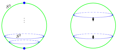
Figure 1: The figure on the left sketches the spherical, maximally symmetric branes in $S^{3}$ in a lower-dimensional illustration. The figure on the right shows a superposition of oriented branes which are related by the antipodal map.

The orientation of the branes is related to the fermionic part of the theory, so the two different implementations of the antipodal map should correspond to two conformal field theory descriptions differing in the way the orbifold acts on the fermions. The first, more natural action of the antipodal map should correspond to an orbifold which acts in the same way on bosons and fermions. It is this model we want to consider here.

The letter is organised as follows. In the next section we specify our model by presenting its field content and analyse the maximally symmetric branes. The corresponding charge group will be computed in section 3. In section 4 we shall construct the boundary state of the brane that wraps the non-trivial one-cycle of SO$(3)$. We shall discuss the relation to the recent K-theory computations by Braun and Schäfer-Nameki [6] in the final section 5.

2 The model and its symmetric branes

The super-symmetric WZNW model on the simply-connected SU$(2)$ is governed by the bosonic currents forming an affine algebra $\text{su}(2)_{k}$ and the fermions which can be combined into currents of an $\text{su}(2)_{2}$ algebra. The modular partition function on the torus is just the diagonal modular invariant of the product theory $\text{su}(2)_{k}\otimes\text{su}(2)_{2}$ . We can label the sectors by an integer $l$ running from $0$ to $k$ and an additional label $s$ from the $\text{su}(2)_{2}$ part taking the values $0,1,2$. The values $s=0,2$ correspond to the NS sector, $s=1$ to the R sector. From the superstring point of view, we can think of the model as a GSO-projected theory of type 0 leaving only NSNS and RR sectors.

The boundary states $|L,S\rangle$ are parametrised by labels with the same range because here we are in the ’Cardy case’ [7] . We can think of the branes with label $S=1$ as an analogue of unstable ’non-BPS’ branes (they do not couple to the closed string RR sector), and the brane with label $|L,2\rangle$ is the anti-brane to the one with label $|L,0\rangle$ (their boundary states only differ in the sign in front of the RR contributions).

The theory we want to consider now is the simple current orbifold of this model with respect to the simple current $(J_{k},J_{2})$ of the product theory, i.e.  the orbifold acts on fermions as well as on the bosonic part. Consistency requires the level $k$ to be even. In the notation of [6], our model is called the $(+)$-twisted model. Note that the $(-)$-twisted model that has been investigated in [1] is the orbifold with respect to the simple current $(J_{k},{\rm id})$ acting only on the bosonic part.

The space of states ${\cal H}$ can be obtained by standard techniques (see e.g. [8]). For $k=4\ell$, we find (Case A)

$${\cal H}\ =\ \bigoplus_{l\text{ even}}{\cal H}_{l}\otimes\overline{{\cal H}}_{l}\otimes({\cal H}_{0}\otimes\overline{{\cal H}}_{0}\oplus{\cal H}_{2}\otimes\overline{{\cal H}}_{2})\ \oplus\bigoplus_{l\text{ odd}}{\cal H}_{l}\otimes\overline{{\cal H}}_{l}\otimes{\cal H}_{1}\otimes\overline{{\cal H}}_{1}\\ \oplus\bigoplus_{l\text{ even}}{\cal H}_{l}\otimes\overline{{\cal H}}_{k-l}\otimes{\cal H}_{1}\otimes\overline{{\cal H}}_{1}\ \oplus\bigoplus_{l\text{ odd}}{\cal H}_{l}\otimes\overline{{\cal H}}_{k-l}\otimes({\cal H}_{0}\otimes\overline{{\cal H}}_{2}\oplus{\cal H}_{2}\otimes\overline{{\cal H}}_{0})\ \ ,$$

and for $k=4\ell-2$ (Case B):

$${\cal H}\ =\ \bigoplus_{l\text{ even}}{\cal H}_{l}\otimes\overline{{\cal H}}_{l}\otimes({\cal H}_{0}\otimes\overline{{\cal H}}_{0}\oplus{\cal H}_{2}\otimes\overline{{\cal H}}_{2})\ \oplus\bigoplus_{l\text{ odd}}{\cal H}_{l}\otimes\overline{{\cal H}}_{l}\otimes{\cal H}_{1}\otimes\overline{{\cal H}}_{1}\\ \oplus\bigoplus_{l\text{ odd}}{\cal H}_{l}\otimes\overline{{\cal H}}_{k-l}\otimes{\cal H}_{1}\otimes\overline{{\cal H}}_{1}\ \oplus\bigoplus_{l\text{ even}}{\cal H}_{l}\otimes\overline{{\cal H}}_{k-l}\otimes({\cal H}_{0}\otimes\overline{{\cal H}}_{2}\oplus{\cal H}_{2}\otimes\overline{{\cal H}}_{0})\ \ .$$

It is well known how to analyse D-branes in orbifold theories (see e.g. [9, 10, 11, 12, 13, 14, 15]), and we shall explicitly work out the boundary states in our model. First, we look for Ishibashi states for the untwisted, maximally symmetric gluing of the SU$(2)$-currents. In both cases, A and B, we find the states $|l,s\rangle\!\rangle$ for $l+s$ even and $l\not=k/2$. In Case A we find in addition the states $|k/2,S\rangle\!\rangle$ for $S=0,1,2$, in Case B we find the sector $(k/2,1)$ with multiplicity two, $|k/2,1;+\rangle\!\rangle$ and $|k/2,1;-\rangle\!\rangle$.

Selection rules in the Ishibashi states give rise to identification rules for the boundary states $|[L,S]\rangle$. The latter are labelled by equivalence classes of pairs $[L,S]$ with $[L,S]=[k-L,2-S]$. For charge issues we are mainly interested in boundary states with label $S=0,2$ (see next section). We can easily see that in this sector there are no fixed-points under the identification, in contrast to the $(-)$-twisted model of [1].

The boundary states for $S=0,2$ are in Case A given by

$$|[L,S]\rangle\ =\ \sqrt{2}\sum_{l+s\ \text{even}}\frac{S^{(k)}_{Ll}S^{(2)}_{Ss}}{\sqrt{S^{(k)}_{0l}S^{(2)}_{0s}}}|l,s\rangle\!\rangle\ \ ,$$ (1)

and in Case B by

$$|[L,S]\rangle\ =\ \sqrt{2}\!\!\!\!\sum_{\begin{array}[]{cc}\scriptstyle l+s\ \text{even}\\[-2.84526pt] \scriptstyle l\not=k/2\end{array}}\!\!\frac{S^{(k)}_{Ll}S^{(2)}_{Ss}}{\sqrt{S^{(k)}_{0l}S^{(2)}_{0s}}}|l,s\rangle\!\rangle+\frac{S^{(k)}_{L\frac{k}{2}}S^{(2)}_{S1}}{\sqrt{S^{(k)}_{0\frac{k}{2}}S^{(2)}_{01}}}\big{(}|\tfrac{k}{2},1;+\rangle\!\rangle+|\tfrac{k}{2},1;-\rangle\!\rangle\big{)}\ \ .$$ (2)

Here, $S^{(k)}$ and $S^{(2)}$ are the modular S-matrices of $\text{su}(2)_{k}$ and $\text{su}(2)_{2}$, respectively.

The Cardy computation shows that the NIMreps for branes with label $S=0,2$ are in both cases

$$n_{(l,s)[L_{1},S_{1}]}{}^{[L_{2},S_{2}]}\ =\ N^{(k)}_{lL_{1}}{}^{L_{2}}N^{(2)}_{sS_{1}}{}^{S_{2}}+N^{(k)}_{(k-l)L_{1}}{}^{L_{2}}N^{(2)}_{(2-s)S_{1}}{}^{S_{2}}\ \ ,$$ (3)

where $N^{(k)}$ and $N^{(2)}$ are the fusion matrices of $\text{su}(2)_{k}$ and $\text{su}(2)_{2}$.

In a superstring theory context, the boundary states obtained from a pure CFT analysis have to be altered slightly (see e.g. [16, 17]) to obtain correct GSO projected open string spectra and to respect space-time spin-statistics. In our case this amounts to an insertion of a factor of $i$ in front of the RR contributions in the boundary states with $S=0,2$. The open string partition function for $S,S^{\prime}=0,2$ is then

$$Z_{[L,S]}{}^{[L^{\prime},S^{\prime}]}(q)\ =\ \sum_{l,s}n_{(l,s)[L,2-S]}{}^{[L^{\prime},S^{\prime}]}\,\chi^{(k)}_{l}(q)\chi^{(2)}_{s}(q)\ \ ,$$ (4)

e.g. the spectrum of a $[0,0]$-brane is

$$Z_{[0,0]}{}^{[0,0]}(q)\ =\ \chi^{(k)}_{0}(q)\chi^{(2)}_{2}(q)+\chi^{(k)}_{k}(q)\chi^{(2)}_{0}(q)\ \ ,$$

and does not contain a tachyon.

3 Charges of symmetric branes

For the charge analysis we can concentrate on the branes with label $[L,0]$ and $[L,2]$ (the boundary states with label $S=1$ do not couple to the RR sector and they always have a tachyon in their spectrum). One way of determining brane charges from the world-sheet point of view is by looking for conserved charges under RG-flows. In WZNW models, this method has been successfully applied in many examples [18, 19, 20, 21] by considering flows described by the Affleck-Ludwig rule [22]. In our case, these flows give rise to the charge constraint

$$\dim(l)\,q_{[L_{1},S_{1}]}\ =\ \sum_{[L_{2},S_{2}]}n_{(l,0)[L_{1},S_{1}]}{}^{[L_{2},S_{2}]}\ q_{[L_{2},S_{2}]}\ \ .$$

Here, $q_{[L,S]}$ is the abelian charge assigned to $[L,S]$, and $\dim(l)=l+1$ is the dimension of the corresponding representation of $\text{su}(2)$. Let us set $S_{1}=0$. From the expression (3) for the NIMrep we find

$$\dim(l)\,q_{[L_{1},0]}\ =\ \sum_{L_{2}}N^{(k)}_{lL_{1}}{}^{L_{2}}\ q_{[L_{2},0]}\ \ .$$

The solution to this charge constraint is well known from the analysis of SU$(2)$ (see e.g. [18, 19]). Without further constraints, the charges would take values in the finite group $\mathcal{C^{\prime}}=\mathbb{Z}_{k+2}$ and they are given by $q_{[L,0]}=\dim(L)$. This is the same charge group as for SU$(2)$. We have to be aware of the problem that there will be many more flows which are not of the Affleck-Ludwig form, and they could restrict the charge group further. It actually turns out that not all the branes are stable. From (4) we see in particular that the brane with label $L=k/2$ has a tachyon (the vacuum state with $l=0,s=0$) in its open string spectrum. Moreover, it does not couple to the closed string RR sector. Put differently, the brane $|[\frac{k}{2},0]\rangle$ corresponds in SU$(2)$ to a superposition of brane and anti-brane, a chargeless configuration that is not stable. We expect that there are RG-flows which lead from a configuration where this superposition is present to one where it has vanished; and these flows should be present also in the SO$(3)$ model. This suggests that the brane $|[\frac{k}{2},0]\rangle$ has charge zero, so $q_{[\frac{k}{2},0]}=\frac{k}{2}+1\stackrel{{\scriptstyle!}}{{=}}0$. We conclude that the charge group of symmetric even-dimensional branes is $\mathcal{C}_{\text{even}}=\mathbb{Z}_{\frac{k+2}{2}}$. Interestingly, this result has been anticipated in [3].

4 Symmetry breaking branes and the non-trivial one-cycle

The branes considered so far preserve as much of the SU$(2)$ symmetry as possible. Branes with less symmetry in SU$(2)$ have been constructed in [23] (see [24, 25] for generalisations to other groups). The simplest of them corresponds geometrically to a 1-dimensional circle [23]. In the usual SU$(2)$ model it is not expected to carry any charge, because there is no non-trivial one-cycle in the simply connected SU$(2)$. In SO$(3)$ on the other hand, we would expect that it is possible for a brane to wrap the non-trivial cycle giving rise to a $\mathbb{Z}_{2}$ charge.

In this section we shall state explicitly the corresponding boundary state. We identify it by its mass and its localisation region. Under the assumption that the symmetry breaking branes in SU$(2)$ do not carry any charges, we show that this brane carries a $\mathbb{Z}_{2}$ charge.

What one usually calls ’symmetry breaking boundary states’ are in truth maximally symmetric boundary states with respect to a smaller symmetry algebra $\mathcal{A}^{\prime}$. Here, we want to break down the maximal chiral algebra $\mathcal{A}=\text{su}(2)_{k}\otimes\text{su}(2)_{2}$ in the following way,

$$\mathcal{A}\ =\ \text{su}(2)_{k}\,\otimes\,\text{su}(2)_{2}\ \longrightarrow\ \text{su}(2)_{k}\,\otimes\,\frac{\text{su}(2)_{2}}{\text{u}(1)_{4}}\,\otimes\,\text{u}(1)_{4}$$

$$\longrightarrow\ \frac{\text{su}(2)_{k}\,\otimes\,\text{u}(1)_{4}}{\text{u}(1)_{2k+4}}\,\otimes\,\text{u}(1)_{2k+4}\,\otimes\,\frac{\text{su}(2)_{2}}{\text{u}(1)_{4}}\ =\ \mathcal{A}^{\prime}\ \ .$$

The sectors can be decomposed with respect to $\mathcal{A}^{\prime}$,

$${\cal H}_{l}\otimes{\cal H}_{s}(q)\ =\ \bigoplus{\cal H}_{[l,s^{\prime},m]}\otimes{\cal H}_{m}\otimes{\cal H}_{[s,s^{\prime}]}\ \ ,$$

where $m$ is a $(2k+4)$-periodic integer which labels sectors of $\text{u}(1)_{2k+4}$, and $s^{\prime}$ is a label of $\text{u}(1)_{4}$ taking the values $s^{\prime}=0,1,2,3$ modulo $4$. The coset sectors are labelled by equivalence classes of tuples with the identifications $[l,s^{\prime},m]=[k-l,s^{\prime}+2,m+k+2]$ and $[s,s^{\prime}]=[2-s,s^{\prime}+2]$. The total space of states then reads

$${\cal H}\ =\ \bigoplus_{\begin{array}[]{cc}\scriptstyle l+s\ \text{even}\\[-2.84526pt] \scriptstyle s_{1}^{\prime},s_{2}^{\prime},m_{1},m_{2}\end{array}}\!\!\!\!{\cal H}_{[l,s_{1}^{\prime},m_{1}]}\otimes{\cal H}_{m_{1}}\otimes{\cal H}_{[s,s_{1}^{\prime}]}\otimes\overline{{\cal H}}_{[l,s_{2}^{\prime},m_{2}]}\otimes\overline{{\cal H}}_{m_{2}}\otimes\overline{{\cal H}}_{[s,s_{2}^{\prime}]}$$

$$\oplus\!\!\! \bigoplus_{\begin{array}[]{cc}\scriptstyle l+s\begin{array}[]{ll}\scriptstyle\text{odd (A)}\\[-4.83694pt] \scriptstyle\text{even (B)}\end{array}\\[-2.84526pt] \scriptstyle s_{1}^{\prime},s_{2}^{\prime},m_{1},m_{2}\end{array}}\!\!\!{\cal H}_{[l,s_{1}^{\prime},m_{1}]}\otimes{\cal H}_{m_{1}}\otimes{\cal H}_{[s,s_{1}^{\prime}]}\otimes\overline{{\cal H}}_{[k-l,s_{2}^{\prime},m_{2}]}\otimes\overline{{\cal H}}_{m_{2}}\otimes\overline{{\cal H}}_{[2-s,s_{2}^{\prime}]}\ \ \ .$$

Now we want to implement gluing conditions which twist the currents of the $u(1)_{2k+4}$. The closed string sectors ${\cal H}_{\dots}\otimes\overline{{\cal H}}_{\dots}$ that can couple to such a boundary state are characterised by

$$[l,s,m]\ =\ [\bar{l},\bar{s},\bar{m}]$$

$$m\ =\ -\bar{m}$$

$$[s,s^{\prime}]\ =\ [\bar{s},\bar{s}^{\prime}]\ \ .$$

It is straightforward to find the list of Ishibashi states, in Case A they are labelled by $|l,s,s^{\prime},m\rangle\!\rangle$ where $m=0,\pm\frac{k+2}{2},k+2$, and $s+s^{\prime}$ as well as $l+s+m$ are even; in Case B the states with $l=\frac{k}{2}$ and $s=1$ occur with multiplicity 2.

For simplicity we only work out the boundary states for Case A. They are labelled by $|[L,S,S^{\prime},\hat{M}]\rangle$. Here, $\hat{M}$ can take the values $0,1,2,3$ and is defined modulo 4. As always, the selection rules on Ishibashi states give rise to identifications among the boundary labels, namely

$$[L,S,S^{\prime},\hat{M}]\ =\ [L,2-S,S^{\prime}+2,\hat{M}]\ =\ [k-L,S,S^{\prime}+2,\hat{M}+2]\ \ .$$

The boundary state reads explicitly

$$|[L,S,S^{\prime},\hat{M}]\rangle\ =\ {\sum}^{\prime}\frac{S^{(k)}_{Ll}}{\sqrt{S^{(k)}_{0l}}}\frac{S^{(2)}_{Ss}}{\sqrt{S^{(2)}_{0s}}}\frac{Z^{(4)}_{S^{\prime}s^{\prime}}}{Z^{(4)}_{0s^{\prime}}}\frac{\psi_{\hat{M}m}}{Z^{(2k+4)}_{0m}}|l,s,s^{\prime},m\rangle\!\rangle$$

where the sum is restricted to the allowed range for the Ishibashi states. We denoted the modular S-matrix of $u(1)_{k}$ by $Z^{(k)}$ to distinguish it from the S-matrix of SU$(2)$. The matrix $\psi$ is defined by

$$\psi_{\hat{M}m}\ =\ \frac{1}{2}\exp\big{(}i\pi m\hat{M}/(k+2)\big{)}\ \ .$$

Now let us look at charges. As for the symmetric case, all branes can be generated from the branes with label $L=0$ , so we shall concentrate on these. The boundary states with label $\hat{M},\hat{M}+2$ arise from a fixed-point resolution of symmetry breaking boundary states in SU$(2)$. If we assume that these branes in SU$(2)$ do not carry any charge, we conclude that the superposition of two branes differing in $\hat{M}$ by 2 is chargeless. On the other hand, branes with different $\hat{M}$ are connected by marginal deformations, and so they have to carry identical charges. This means that symmetry-breaking branes in SO$(3)$ can at most carry a $\mathbb{Z}_{2}$ charge.

The geometric interpretation of these symmetry-breaking branes can be inferred from the general rules given in [23, 24]. It stretches along the image of the $S^{1}$ sitting inside SU$(2)$ and passing through $-{\rm id}$, and hence it wraps the non-trivial one-cycle. We can ask whether it really wraps the cycle once. The answer is yes which can be seen from the following analysis of masses. The length of the cycle is $\pi R$ where $R\sim\sqrt{k}$ is the radius of the SU$(2)$ (we set $\alpha^{\prime}=1$). The tension of the D1-brane is $\frac{1}{2\pi}$, so the ratio of its mass and the mass of the D0-brane (which is described by the boundary state $|[0,0]\rangle$ of (1)) is

$$\frac{\text{Mass of D1-brane on one-cycle}}{\text{Mass of D0-brane}}\ \sim\ \frac{\sqrt{k}}{2}\ \ .$$

This should be compared to the ratio of g-factors of the boundary states,

$$\frac{g_{|[0,0,0,0]\rangle}}{g_{|[0,0]\rangle}}\ =\ \frac{\psi_{00}}{\sqrt{2}Z^{(2k+4)}_{00}}\ =\ \frac{\sqrt{k+2}}{2}\ \ .$$

Having in mind that the geometric interpretation applies for large values of the level $k$, we find complete agreement.

5 Discussion

Let us summarise our results. We analysed brane charges in the $(+)$-twisted model of SO$(3)$. The charge groups of even-dimensional, maximally symmetric branes and the contribution of the odd-dimensional symmetry breaking branes are

$$\mathcal{C}_{\text{even}}\ =\ \mathbb{Z}_{\frac{k+2}{2}} \mathcal{C}_{\text{odd}}\ =\ \mathbb{Z}_{2}\ \ .$$ (5)

There is much evidence that D-brane charges are classified by K-theory [28, 29]. For branes in backgrounds $X$ with a non-trivial NSNS 3-form field $H$, one has to use twisted K-groups ${}^{H}\!K(X)$ [30, 31]. This applies in particular to WZNW models where the corresponding K-theories for simply-connected group manifolds have been computed in [32, 33]. Recently, Braun and Schäfer-Nameki computed the twisted K-theory of SO$(3)$ [6]. The authors found two possible answers ${}^{(\pm,H)}K^{*}(\text{SO}(3))$ depending on the choice of a twist in $H^{1}(\text{SO}(3),\mathbb{Z}_{2})$. One version, ${}^{(-,H)}K^{*}(\text{SO}(3))$, is in agreement with the results of [1] for the $(-)$-twisted model. The other K-groups are

$${}^{(+,H)}K^{1}(\text{SO}(3))\ =\ \mathbb{Z}_{\frac{k+2}{2}} {}^{(+,H)}K^{0}(\text{SO}(3))\ =\ \mathbb{Z}_{2}\ \ .$$

Obviously, these results agree exactly with the charge groups $\mathcal{C}_{\text{even}}$ and $\mathcal{C}_{\text{odd}}$ in eq. (5).

Let us shortly comment on the role of the symmetry-breaking branes. In SU$(2)$ and SO$(3)$, these are objects of even co-dimension, and their charge should be measured by $K^{0}$. In our $(+)$-twisted model, we found a D1-brane wrapping the non-trivial one-cycle which contributes a $\mathbb{Z}_{2}$-charge in agreement with the K-group ${}^{(+,H)}K^{0}(\text{SO}(3))$ above. For the other twist, the result of [6] is ${}^{(-,H)}K^{0}(\text{SO}(3))=0$. In the analysis of the corresponding conformal field theory model in [1], symmetry breaking branes have not been considered, and at first sight one might think that one finds a D1 on the non-trivial cycle along the same lines as in section 4. This is not the case. An analysis of masses reveals that a similar construction in the $(-)$-twisted model only gives rise to D1-branes which wrap the cycle twice. The reason is simple: in the $(+)$-twisted model, the D1-brane of SU$(2)$ is fixed under the antipodal map and gets resolved in SO$(3)$. In the $(-)$-twisted model on the other hand the D1-brane of SO$(3)$ corresponds to a superposition of two D1-branes of different orientations. Therefore, it is contractible and we do not expect it to carry any charge; again, we find agreement with the K-theory result.

This special analysis for $\text{SO}(3)\sim\text{SU}(2)/\mathbb{Z}_{2}$ can be generalised to orbifolds of higher rank groups. In [1], brane charges are analysed in the models $\frac{\text{su}(n)_{k}}{\mathbb{Z}_{m}}\otimes\text{so}(d)_{1}$ where $d=n^{2}-1$ is the dimension of SU$(n)$. Instead one could analyse the theories $\frac{\text{su}(n)_{k}\otimes\,\text{so}(d)_{1}}{\mathbb{Z}_{m}}$. The action of $\mathbb{Z}_{m}$ on SU$(n)$ induces a natural action of $\mathbb{Z}_{m}$ on SO$(d)$. It turns out that this action on the fermions is non-trivial only if $n$ is even and $n/m$ is odd, and here we would expect new phenomena. These are precisely the ’pathological cases’ in the analysis of [1] where the order of the charge group is unexpectedly small and does not grow with the level $k$. Therefore we suggest that one should repeat the charge analysis in these cases with the changed orbifold action. For comparison, it would be very interesting to compute the corresponding K-groups.

Acknowledgements

I would like to thank Pedro Bordalo, Volker Braun, Matthias Gaberdiel, Terry Gannon, Sakura Schäfer-Nameki and Volker Schomerus for useful discussions and correspondences.

References

- [1] M. R. Gaberdiel, T. Gannon, D-brane charges on non-simply connected groups (2004), hep-th/0403011
- [2] G. Felder, J. Fröhlich, J. Fuchs, C. Schweigert, The geometry of WZW branes, J. Geom. Phys. 34 (2000) 162, hep-th/9909030
- [3] K. Matsubara, V. Schomerus, M. Smedbäck, Open strings in simple current orbifolds, Nucl. Phys. B626 (2002) 53, hep-th/0108126
- [4] N. Couchoud, D-branes and orientifolds of SO(3), JHEP 03 (2002) 026, hep-th/0201089
- [5] P. Bordalo, A. Wurtz, D-branes in lens spaces, Phys. Lett. B568 (2003) 270, hep-th/0303231
- [6] V. Braun, S. Schäfer-Nameki, Supersymmetric WZW models and twisted K-theory of SO(3) (2004), hep-th/0403287
- [7] J. L. Cardy, Boundary conditions, fusion rules and the Verlinde formula, Nucl. Phys. B324 (1989) 581
- [8] P. D. Francesco, P. Mathieu, D. Sénéchal, Conformal Field Theory, Graduate Texts in Contemporary Physics, Springer, New York (1999)
- [9] G. Pradisi, A. Sagnotti, Open string orbifolds, Phys. Lett. B216 (1989) 59
- [10] G. Pradisi, A. Sagnotti, Y. S. Stanev, The Open descendants of nondiagonal SU(2) WZW models, Phys. Lett. B356 (1995) 230, arXiv:hep-th/9506014
- [11] M. R. Douglas, G. W. Moore, D-branes, Quivers, and ALE Instantons (1996), hep-th/9603167
- [12] J. Fuchs, C. Schweigert, Orbifold analysis of broken bulk symmetries, Phys. Lett. B447 (1999) 266, hep-th/9811211
- [13] J. Fuchs, C. Schweigert, Symmetry breaking boundaries. I: General theory, Nucl. Phys. B558 (1999) 419, hep-th/9902132
- [14] L. Birke, J. Fuchs, C. Schweigert, Symmetry breaking boundary conditions and WZW orbifolds, Adv. Theor. Math. Phys. 3 (1999) 671, hep-th/9905038
- [15] R. E. Behrend, P. A. Pearce, V. B. Petkova, J.-B. Zuber, Boundary conditions in rational conformal field theories, Nucl. Phys. B570 (2000) 525, hep-th/9908036
- [16] A. Recknagel, V. Schomerus, D-branes in Gepner models, Nucl. Phys. B531 (1998) 185, hep-th/9712186
- [17] M. Billo, B. Craps, F. Roose, Orbifold boundary states from Cardy’s condition, JHEP 01 (2001) 038, hep-th/0011060
- [18] A. Alekseev, V. Schomerus, RR charges of D2-branes in the WZW model (2000), hep-th/0007096
- [19] S. Fredenhagen, V. Schomerus, Branes on group manifolds, gluon condensates, and twisted K-theory, JHEP 04 (2001) 007, hep-th/0012164
- [20] P. Bouwknegt, P. Dawson, D. Ridout, D-branes on group manifolds and fusion rings, JHEP 12 (2002) 065, hep-th/0210302
- [21] M. R. Gaberdiel, T. Gannon, The charges of a twisted brane, JHEP 01 (2004) 018, hep-th/0311242
- [22] I. Affleck, A. W. W. Ludwig, The Kondo effect, conformal field theory and fusion rules, Nucl. Phys. B352 (1991) 849
- [23] J. Maldacena, G. W. Moore, N. Seiberg, Geometrical interpretation of D-branes in gauged WZW models, JHEP 07 (2001) 046, hep-th/0105038
- [24] T. Quella, V. Schomerus, Symmetry breaking boundary states and defect lines, JHEP 06 (2002) 028, hep-th/0203161
- [25] T. Quella, On the hierarchy of symmetry breaking D-branes in group manifolds, JHEP 12 (2002) 009, hep-th/0209157
- [26] S. Fredenhagen, V. Schomerus, On boundary RG-flows in coset conformal field theories, Phys. Rev. D67 (2003) 085001, hep-th/0205011
- [27] S. Fredenhagen, Organizing boundary RG flows, Nucl. Phys. B660 (2003) 436, hep-th/0301229
- [28] R. Minasian, G. Moore, K-theory and Ramond-Ramond charge, JHEP 11 (1997) 002, hep-th/9710230
- [29] E. Witten, D-branes and K-theory, JHEP 12 (1998) 019, hep-th/9810188
- [30] A. Kapustin, D-branes in a topologically nontrivial B-field, Adv. Theor. Math. Phys. 4 (2000) 127, hep-th/9909089
- [31] P. Bouwknegt, V. Mathai, D-branes, B-fields and twisted K-theory, JHEP 03 (2000) 007, hep-th/0002023
- [32] J. M. Maldacena, G. W. Moore, N. Seiberg, D-brane instantons and K-theory charges, JHEP 11 (2001) 062, hep-th/0108100
- [33] V. Braun, Twisted K-theory of Lie groups, JHEP 03 (2004) 029, hep-th/0305178