On Correspondences Between Toric Singularities
and $(p,q)$-webs

Abstract:

We study four-dimensional ${\cal N}=1$ gauge theories which arise from D3-brane probes of toric Calabi-Yau threefolds. There are some standing paradoxes in the literature regarding relations among $(p,q)$-webs, toric diagrams and various phases of the gauge theories, we resolve them by proposing and carefully distinguishing between two kinds of $(p,q)$-webs: toric and quiver $(p,q)$-webs. The former has a one to one correspondence with the toric diagram while the latter can correspond to multiple gauge theories. The key reason for this ambiguity is that a given quiver $(p,q)$-web can not capture non-chiral matter fields in the gauge theory. To support our claim we analyse families of theories emerging from partial resolution of Abelian orbifolds using the Inverse Algorithm of hep-th/0003085 as well as $(p,q)$-web techniques. We present complex inter-relations among these theories by Higgsing, blowups and brane splittings. We also point out subtleties involved in the ordering of legs in the $(p,q)$ diagram.

1 Introduction and Summary

Investigating the world volume theories of D-brane probes on Calabi-Yau manifolds is of vital phenomenological importance as well as theoretical interest. In particular, toric singularities have been investigated for some time [1, 2, 3, 4, 5, 6] because of the wealth of mathematical techniques that allow a detailed study. Amongst many other boons, progress in this direction has taught us salient prospects on the AdS/CFT correspondence [2, 21, 22, 23].

A plethora of methods have been developed to extract field theories from these toric singularities, each with its virtues. The first of these methods is to use the so-called “Inverse Algorithm” developed in [7, 8, 9]. This algorithm is based on the “Forward Algorithm” given in [1, 5, 6]. Another method is to use the higgsing mechanism, starting from a parent Abelian orbifold theory and adjusting the FI-parameters properly in the spacetime field theory [12, 13, 14, 20]. A third method is to use geometric engineering techniques of [17] to calculate the appropriate intersection numbers and mappings among exceptional collections [15, 16, 22, 28]. The fourth one, which we shall address in detail here, is to use the $(p,q)$-web picture of [31, 32] as a useful guide to directly obtain the matter content and find fields which should be higgsed down [15, 18]. Of these four methods, the $(p,q)$-web technique is very attractive, given the ease by which the matter content, i.e., quiver diagram, of the gauge theory can be calculated (from intersection numbers of $(p,q)$-charges) and the immediate identification of fields higgsed down by acquiring VEVs in the parent orbifold theory.

For toric singularities, the method of $(p,q)$-webs is particularly useful due to a supposed equivalence between the toric diagram and the $(p,q)$-web representations [31, 32]. The $(p,q)$ webs provide us with a very direct and picturesque perspective. Indeed, in [31], it was noticed that the grid diagram dual to $(p,q)$-web precisely resembles the corresponding toric diagram. Then, in [32], evidence from the geometric point of view was given to support such a relation. These works tell us that (at least for the case of a single interior point in the toric diagram) there is a one-to-one correspondence between the $(p,q)$-web and the toric data.

If we accept the above correspondence, the next question is to find the quiver theory of a given toric data or $(p,q)$-web. As mentioned above, the quiver diagram can be directly obtained from the given $(p,q)$ charges. The relation between the quiver diagram and the $(p,q)$ charges was established in [15] by mirror symmetry for cones over del Pezzo surfaces. This begs the question: does a one-to-one correspondence hold for general $(p,q)$-webs? Along this line, [18] identified different $(p,q)$-webs for different phases of toric duality [7, 8] for cones over the ample surfaces $F_{0}$, $dP_{2}$ and $dP_{3}$ and established the transitions among them by higgsing and unhiggsing mechanisms [20].

Therefore, we run into a paradox. On the one hand, a one-to-one correspondence would dictate that given a toric singularity, there should be a unique corresponding $(p,q)$-web. On the other hand, different $(p,q)$-webs have been identified with different toric (Seiberg) dual phases of a given toric singularity. The two situations cannot both be true and yet each seems to have its supporting evidence.

It is the main aim of this paper to explain this puzzle. By careful analysis, we find that we need to distinguish two kinds of $(p,q)$-webs. The first one is what we shall call a toric $(p,q)$-web which has the direct one-to-one correspondence with a given toric variety. This is the one considered in [15, 31, 32]. The second one is what we shall call quiver $(p,q)$-web which re-expresses a quiver diagram in the form of a $(p,q)$-web [18]. The second concept has limitations. Firstly, the quiver $(p,q)$-web can be applied only for toric diagrams with one interior point. For those with more than one interior point, we need to use more than one pair of $(p,q)$ charges to calculate the quiver diagram. Secondly, as we will show, we can use the same “quiver $(p,q)$-web” for several different theories and read out various higgsing phases; this will circumvent our problem of the lack of one-one correspondence. Because of these limitations, however, we think that the first concept of the toric $(p,q)$-web is more fundamental, although the second does have its useful rôle.

In summary, then, the outline of the paper is as follows. We begin with a review in Section 2 on the key points of $(p,q)$-webs and in particular how they represent a four-dimensional world-volume gauge theory on D3-branes probing singular toric Calabi-Yau varieties. We show how one obtains the web from the toric diagram of the singularity by graph-dualisation. Such webs we shall call “toric $(p,q)$-webs.” We then go to extensive case studies of the toric partial resolutions of $\hbox{$\,\vrule height=6.45831pt,width=0.4pt,depth=0.0pt\kern-3.00003pt{\rm C}$}^{3}/\mathchoice{\hbox{\cmss Z\kern-3.99994ptZ}}{\hbox{\cmss Z\kern-3.99994ptZ}}{\lower 0.9pt\hbox{\cmsss Z\kern-2.79996ptZ}}{\lower 1.2pt\hbox{\cmsss Z\kern-2.79996ptZ}}_{3}\times\mathchoice{\hbox{\cmss Z\kern-3.99994ptZ}}{\hbox{\cmss Z\kern-3.99994ptZ}}{\lower 0.9pt\hbox{\cmsss Z\kern-2.79996ptZ}}{\lower 1.2pt\hbox{\cmsss Z\kern-2.79996ptZ}}_{3}$ in Section 3. We will reach families of Hirzebruch, del Pezzo and so-called pseudo del Pezzo surfaces. The quivers for these theories are intricately inter-related and if we ignored bi-directional arrows therein many of these theories have the same quiver even though their toric diagrams and hence toric $(p,q)$-webs differ greatly. We re-construct the web which gives rise to these quivers and call these webs “quiver $(p,q)$-webs.” These are more useful in reading out the higgsing information. To this we then turn in Section 4 where detailed checks from the field theory, complete with the superpotential, are carried out to show how these plethora of theories are related by (un)higgsing. From the web point of view, these (un)higgsing correspond to splitting and combining of external legs in the web-diagrams, and we finally show how the various theories can be reached by combining legs from the parent $(p,q)$-webs of the $\hbox{$\,\vrule height=6.45831pt,width=0.4pt,depth=0.0pt\kern-3.00003pt{\rm C}$}^{3}/\mathchoice{\hbox{\cmss Z\kern-3.99994ptZ}}{\hbox{\cmss Z\kern-3.99994ptZ}}{\lower 0.9pt\hbox{\cmsss Z\kern-2.79996ptZ}}{\lower 1.2pt\hbox{\cmsss Z\kern-2.79996ptZ}}_{3}\times\mathchoice{\hbox{\cmss Z\kern-3.99994ptZ}}{\hbox{\cmss Z\kern-3.99994ptZ}}{\lower 0.9pt\hbox{\cmsss Z\kern-2.79996ptZ}}{\lower 1.2pt\hbox{\cmsss Z\kern-2.79996ptZ}}_{3}$ orbifold.

2 A Brief Reminder on $(p,q)$-Webs of Branes

We are interested in the construction of a wide class of four-dimensional ${\cal N}=1$ gauge theories that arise on the world-volume of D-branes probing toric singularities. A particularly visual method of studying the quiver that arise from such theories is to use $(p,q)$-webs. In this section, we briefly outline the techniques involved before proceeding on to study detailed examples. The reader is encouraged to also refer to Section 2 of [18] for a very nice review on this subject in the present context.

2.1 The $(p,q)$-Web

We first recall that the S-duality in type IIB, or equivalently, the torus modular group in F-theory, allows the existence of $(p,q)$ branes. The D5-brane is assigned a charge of $(1,0)$ while the NS5-brane has charge $(0,1)$. The methods of [29, 30] allowed [31, 32] to construct five-dimensional ${\cal N}=1$ theories via configurations of type IIB $(p,q)$-fivebranes, stretched in a way such that 4+1 common dimensions of the world-volume correspond to spacetime for the gauge theory. In the transverse 5 directions the branes look like lines which conjoin in a web fashion. We therefore suppress 3 of the transverse direction and represent our branes as intersections of lines in a two-dimensional coördinate system with axes $(p,q)$ so that the charge of the $(p,q)$ fivebrane can be readily read out from its slope. To such configurations we shall refer as $(p,q)$-webs of fivebranes.

The branes intersect at a basic 3-valence vertex which we have drawn in Part (a) of Figure 1. In general, the branes will extend in a skeletal structure woven by 3-valence vertices at which $(p,q)$-charges are conserved. That is, at each vertex, the sum of the $(p,q)$-vectors vanishes. Furthermore, there are internal lines and external lines, the former of which has no free ends; these are colour and flavour branes respectively. An archetypal example of the web is given in Part (b) of Figure 1. In general, a web with $N_{c}$ parallel internal lines and $N_{f}$ external lines corresponds to an $SU(N_{c})$ theory with $N_{f}$ flavours.

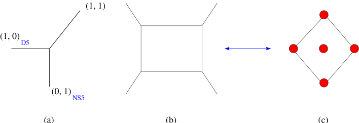
Figure 1: (a) The triple vertex of a D5-brane (1,0), an NS5-brane (0,1) and a (1,1)-brane; (b) An archetypal example of a $(p,q)$-web and (c) its dual grid (toric) diagram.

The Higgs branch of the gauge theory is parametrised by the abovementioned three suppressed dimensions, while the Coulomb branch corresponds to deformations of the relative positions of the $(p,q)$-branes. In (b) of Figure 1, fundamental strings stretched between the parallel fivebranes are BPS states: those between the horizontal correspond to W-bosons of mass $T_{s}\Delta y$ and those between the vertical, instantons of mass $|\tau|T_{s}\Delta x$ (where $\tau$ is the type IIB scalar and $T_{s}$, the fundamental string tension).

The number of global deformations of the theory is $SO(3)$ coming from the Higgs branch; in addition there are

$$n_{G}=\#(\mbox{external faces})-3$$

extra global deformations. On the other hand, the number of local deformations is

$$n_{L}={\rm dim}(\mbox{Coulomb Branch})=\#(\mbox{internal faces})\ .$$

2.2 Grid Diagrams, Toric Diagrams and Four-dimensional Gauge Theory

Having explained the fundamental rules of the representing five-dimensional gauge theories with $(p,q)$-webs. We now explain how this configuration gives rise to a four-dimensional ${\cal N}=1$ gauge theory, which is in particular a world-volume theory of a D3-brane probe of a toric singularity. For some rudiments of toric geometry in the present context, the reader could read, for example, [24]. We point out that, of course, the toric diagrams we draw should be three-dimensional because we are dealing with complex threefolds. However, since we are dealing with local Calabi-Yau threefolds, we henceforth draw only the two-dimensional cross section of the toric diagram. The endpoints of the vectors are coplanar due to the Calabi-Yau condition.

As explained in [31], one could define a dual diagram to the $(p,q)$-web, a so-called grid diagram. The duality is in the sense of finite planar graphs, where vertices and faces are interchanged and edges, to their perpendiculars. This procedure is illustrated in going from our prototypical example (b) to its dual in (c) in Figure 1. The astute reader may recognise (c) to be nothing but a toric diagram; this is precisely the point of [31, 32]. The Inverse Algorithm of [7] was devised exactly for taking this data to gauge theory data in terms of quiver diagrams.

Indeed, in the perspective of [32], it was noted that when geometrically engineering gauge theories from toric varieties, a simple correspondence exists between the geometry and branes. The key features of toric varieties are captured by when the torus fibrations shrink. However, this is precisely where the shrinking cycles become a source of the brane-charges. Therefore these loci should be identified with appropriate brane configurations. To be specific, we have identified lines in the $(p,q)$-web with D5-branes. In addition, there could be (fractional) D3 and D7 branes. Then, the D3-branes can be associated with vertices and D7, with the faces. In other words, we let D3, D5 and D7 branes wrap 0, 2 and 4 cycles respectively in a Calabi-Yau threefold geometry. The result, is a four-dimensional gauge theory, which, on the D3-brane world volume perspective, is the ${\cal N}=1$, four-dimensional quiver gauge theory from probing the said Calabi-Yau, which is a (non-compact) toric variety whose toric diagram is specified by the grid diagram.

In light of these insights, obtaining the matter content of the ${\cal N}=1$ gauge theories on D-branes probing toric singularities can be extremely intuitive and straight-forward. Indeed, given the toric diagram, one simply has to identify it with a grid diagram, and then draw the dual; this is then the $(p,q)$-web. Assigning appropriate $(p_{i},q_{i})$-charges to each external leg $i$ according to the direction of the vectors, the quiver matrix of the resulting theory is instantly given by

$$\chi_{ij}=\det\left(\matrix{p_{i}&p_{j}\cr q_{i}&q_{j}}\right)\ .$$ (2.1)

Of course, there are limitations to this methodology: in contrast to the generality of the Inverse Algorithm of [7], there is a present lack of a direct method to obtain the superpotential. Moreover, subtleties arise when there are multiple internal points (or equivalently, parallel external legs). More pertinent to us is the fact that we see that (2.1) is naturally antisymmetric in the indices $i$ and $j$. The non-antisymmetric parts are (1) adjoint matter corresponding to non-zero diagonal entries in the quiver matrix and (2) non-chiral matter corresponding to bi-directional arrows, i.e., symmetric parts, in the quiver matrix. Capturing these fields, though being discussed nicely in [15], still lacks a systematic analysis from geometric methods such as $(p,q)$-webs.

An important point is that the $(p,q)$-web method culminating in (2.1) seems to suggest a one-to-one correspondence between the toric data and the $(p,q)$-web data in the sense that they are dual finite graphs. Once the toric diagram is given, the $(p,q)$-web, and thence the quiver, are uniquely determined. We will point below how one needs to be careful with this identification and emphasise the concepts of “toric” versus “quiver” $(p,q)$-webs.

3 Case Studies: Partial Resolutions of $\hbox{$\,\vrule height=6.45831pt,width=0.4pt,depth=0.0pt\kern-3.00003pt{\rm C}$}^{3}/\mathchoice{\hbox{\cmss Z\kern-3.99994ptZ}}{\hbox{\cmss Z\kern-3.99994ptZ}}{\lower 0.9pt\hbox{\cmsss Z\kern-2.79996ptZ}}{\lower 1.2pt\hbox{\cmsss Z\kern-2.79996ptZ}}_{3}\times\mathchoice{\hbox{\cmss Z\kern-3.99994ptZ}}{\hbox{\cmss Z\kern-3.99994ptZ}}{\lower 0.9pt\hbox{\cmsss Z\kern-2.79996ptZ}}{\lower 1.2pt\hbox{\cmsss Z\kern-2.79996ptZ}}_{3}$

We will be focusing on the D-brane probe theories that arise from partial resolutions of Abelian orbifolds, especially the cones of the Hirzebruch and del Pezzo surfaces; these have readily available data from the Inverse Algorithm with which we may compare and contrast. Some of these have been very nicely considered in [15, 18] from the $(p,q)$ point of view.

The gauge theories on D-brane probes to partial resolutions of the Abelian orbifold $\hbox{$\,\vrule height=6.45831pt,width=0.4pt,depth=0.0pt\kern-3.00003pt{\rm C}$}^{3}/\mathchoice{\hbox{\cmss Z\kern-3.99994ptZ}}{\hbox{\cmss Z\kern-3.99994ptZ}}{\lower 0.9pt\hbox{\cmsss Z\kern-2.79996ptZ}}{\lower 1.2pt\hbox{\cmsss Z\kern-2.79996ptZ}}_{3}\times\mathchoice{\hbox{\cmss Z\kern-3.99994ptZ}}{\hbox{\cmss Z\kern-3.99994ptZ}}{\lower 0.9pt\hbox{\cmsss Z\kern-2.79996ptZ}}{\lower 1.2pt\hbox{\cmsss Z\kern-2.79996ptZ}}_{3}$ have been extensively studied [5, 7]; the Inverse Algorithm of [7] and subsequent duality considerations [8, 9, 10, 11, 12, 20] have provided us with a wealth of explicit examples. The $(p,q)$-web techniques reviewed in the previous Section have been applied to these examples in [18].

In this section, we will re-examine these examples together with some new ones, in order to demonstrate that there are really two kinds of $(p,q)$-webs. In particular we will focus on the cones over Hirzebruch surfaces and so-called pseudo-del Pezzo surfaces.

3.1 The $F_{2}$ Singularity

We begin with an example not previously addressed in the literature. This is the affine cone $F_{2}$ over the second Hirzebruch surface. The surface itself is a ${\rm I\kern-1.79993ptP}^{1}$-fibration over ${\rm I\kern-1.79993ptP}^{1}$. $F_{2}$ is a local Calabi-Yau threefold which can be described as a singular affine variety. The toric diagram (with a perpendicular dimension of the cone suppressed) for $F_{2}$ is given in part (b) of Figure 2. The background configuration of blue dots is the familiar toric diagram of $\hbox{$\,\vrule height=6.45831pt,width=0.4pt,depth=0.0pt\kern-3.00003pt{\rm C}$}^{3}/\mathchoice{\hbox{\cmss Z\kern-3.99994ptZ}}{\hbox{\cmss Z\kern-3.99994ptZ}}{\lower 0.9pt\hbox{\cmsss Z\kern-2.79996ptZ}}{\lower 1.2pt\hbox{\cmsss Z\kern-2.79996ptZ}}_{3}\times\mathchoice{\hbox{\cmss Z\kern-3.99994ptZ}}{\hbox{\cmss Z\kern-3.99994ptZ}}{\lower 0.9pt\hbox{\cmsss Z\kern-2.79996ptZ}}{\lower 1.2pt\hbox{\cmsss Z\kern-2.79996ptZ}}_{3}$. We see that there is an embedding of toric diagrams. This means that the Inverse Algorithm of [7] can be applied.

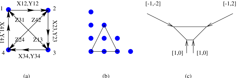
Figure 2: The theory for the singularity $F_{2}$ which is a cone over the second Hirzebruch surface: (a) the quiver diagram; (b) the toric diagram (bounded by the lines) given as an embedding into that of $\hbox{$\,\vrule height=6.45831pt,width=0.4pt,depth=0.0pt\kern-3.00003pt{\rm C}$}^{3}/\mathchoice{\hbox{\cmss Z\kern-3.99994ptZ}}{\hbox{\cmss Z\kern-3.99994ptZ}}{\lower 0.9pt\hbox{\cmsss Z\kern-2.79996ptZ}}{\lower 1.2pt\hbox{\cmsss Z\kern-2.79996ptZ}}_{3}\times\mathchoice{\hbox{\cmss Z\kern-3.99994ptZ}}{\hbox{\cmss Z\kern-3.99994ptZ}}{\lower 0.9pt\hbox{\cmsss Z\kern-2.79996ptZ}}{\lower 1.2pt\hbox{\cmsss Z\kern-2.79996ptZ}}_{3}$; (c) the corresponding $(p,q)$-web diagram.

Subsequently, we can readily obtain the world volume theory of a brane probing $F_{2}$. The matter content is given by the quiver diagram depicted in part (a) of Figure 2; it is a theory with 4 product gauge groups and 12 bi-fundamental fields. The superpotential is given by

$$W_{F_{2}} = X_{12}Y_{23}Z_{31}-Y_{12}X_{23}Z_{31}+X_{23}Y_{34}Z_{41}-Y_{23}X_{34}Z_{41}$$

$$+ X_{34}Y_{41}Z_{13}-Y_{34}X_{41}Z_{13}+X_{41}Y_{12}Z_{24}-Y_{41}X_{12}Z_{24}\ .$$

As discussed above, instead of using the Inverse Algorithm, the matter content, at least, can be easily obtained from a $(p,q)$-web configuration. We dualise the toric diagram to obtain the web; the result is presented in part (c) of Figure 2 with the $(p,q)$-charges appropriately labelled. The quiver is then obtained by the intersection rule (2.1) from the $(p,q)$-charges. The answer is in perfect agreement with that obtained from the Inverse Algorithm, presented in Part (a) of the figure.

Note that the procedure of obtaining the web from the toric diagram involves a direct dualisation of the graph. We henceforth call a web obtained this way a toric $(p,q)$-web to reflect the fact that it is directly and uniquely obtained from the toric diagram by graph-dualisation.

Now, in presenting the quiver and the superpotential, we have purposefully chosen the notations above. The reader may instantly recognise, upon observing the theory presented in the said manner, that the theory is nothing other than the familiar theory of the Abelian orbifold $\hbox{$\,\vrule height=6.45831pt,width=0.4pt,depth=0.0pt\kern-3.00003pt{\rm C}$}^{3}/\mathchoice{\hbox{\cmss Z\kern-3.99994ptZ}}{\hbox{\cmss Z\kern-3.99994ptZ}}{\lower 0.9pt\hbox{\cmsss Z\kern-2.79996ptZ}}{\lower 1.2pt\hbox{\cmsss Z\kern-2.79996ptZ}}_{4}$ with action $(1,1,2)$. That is, with the action of the $\mathchoice{\hbox{\cmss Z\kern-3.99994ptZ}}{\hbox{\cmss Z\kern-3.99994ptZ}}{\lower 0.9pt\hbox{\cmsss Z\kern-2.79996ptZ}}{\lower 1.2pt\hbox{\cmsss Z\kern-2.79996ptZ}}_{4}$ on the coördinates $(x,y,z)$ of $\hbox{$\,\vrule height=6.45831pt,width=0.4pt,depth=0.0pt\kern-3.00003pt{\rm C}$}^{3}$ as $(x,y,z)\rightarrow(\omega_{4}x,\omega_{4}y,\omega_{4}^{2}z)$, where $\omega_{4}$ is the primitive fourth root of unity. Quivers for Abelian orbifolds are most conveniently given in terms of the Brane Box Model representation [25]. For comparison, we have drawn the Brane Box Model of this theory in Figure 3.

$A=\left(\matrix{0&2&1&0\cr 0&0&2&1\cr 1&0&0&2\cr 2&1&0&0}\right),\qquad\qquad\qquad\begin{array}[]{r}\epsfbox{F2box.eps}\hfil\end{array}$

Figure 3: The Brane Box model of for the orbifold theory $\hbox{$\,\vrule height=6.45831pt,width=0.4pt,depth=0.0pt\kern-3.00003pt{\rm C}$}^{3}/\mathchoice{\hbox{\cmss Z\kern-3.99994ptZ}}{\hbox{\cmss Z\kern-3.99994ptZ}}{\lower 0.9pt\hbox{\cmsss Z\kern-2.79996ptZ}}{\lower 1.2pt\hbox{\cmsss Z\kern-2.79996ptZ}}_{4}$ with action $(1,1,2)$. We have also included the adjacency matrix $A$ for reference.

Regarding this equivalence to the orbifold theory, we remark that in general, the toric diagram for $\hbox{$\,\vrule height=6.45831pt,width=0.4pt,depth=0.0pt\kern-3.00003pt{\rm C}$}^{3}/\mathchoice{\hbox{\cmss Z\kern-3.99994ptZ}}{\hbox{\cmss Z\kern-3.99994ptZ}}{\lower 0.9pt\hbox{\cmsss Z\kern-2.79996ptZ}}{\lower 1.2pt\hbox{\cmsss Z\kern-2.79996ptZ}}_{1+a+b}$ with action $(1,a,b)$ is given in Figure 4.

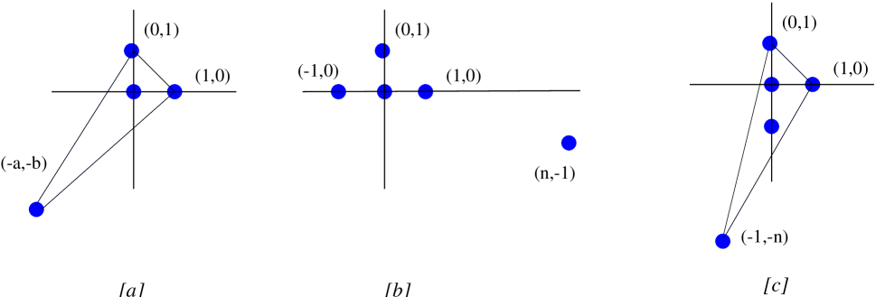
Figure 4: (a) The toric diagram of the weighted projective space ${\rm I\kern-1.79993ptP}^{2}_{[1,a,b]}$, which is the exceptional divisor in the resolution of the abelian orbifold $\hbox{$\,\vrule height=6.45831pt,width=0.4pt,depth=0.0pt\kern-3.00003pt{\rm C}$}^{3}/\mathchoice{\hbox{\cmss Z\kern-3.99994ptZ}}{\hbox{\cmss Z\kern-3.99994ptZ}}{\lower 0.9pt\hbox{\cmsss Z\kern-2.79996ptZ}}{\lower 1.2pt\hbox{\cmsss Z\kern-2.79996ptZ}}_{1+a+b}$ with action $(1,a,b)$. (b) The toric diagram of the $n$-th Hirzebruch surface. (c) We redraw (a) for the case of ${\rm I\kern-1.79993ptP}^{2}_{[1,1,n]}$ and see that toric diagram, up to rotation, coincides with that of (b).

This toric diagram, when visualized in the two-dimensional cross section, is that of the weighted projective space ${\rm I\kern-1.79993ptP}^{2}_{[1,a,b]}$. This fact was observed in [10], and the corresponding “toric” $(p,q)$-web has also been constructed therein. Indeed for large $(a,b)$, there may be multiple interior points. This would therefore be an example which demonstrates that the one-to-one correspondence, in the sense of dual graphs, between the toric $(p,q)$-web and the toric diagram is still valid even with multiple inner points in the toric diagram. The web diagram can also be used to investigate the resolution of singularities, as discussed in [10].

More importantly, we have that the quiver obtained from (2.1) for $F_{n\geq 2}$, the cone over the $n$-th Hirzebruch surface, is given simply by that of the Abelian orbifold $\hbox{$\,\vrule height=6.45831pt,width=0.4pt,depth=0.0pt\kern-3.00003pt{\rm C}$}^{3}/\mathchoice{\hbox{\cmss Z\kern-3.99994ptZ}}{\hbox{\cmss Z\kern-3.99994ptZ}}{\lower 0.9pt\hbox{\cmsss Z\kern-2.79996ptZ}}{\lower 1.2pt\hbox{\cmsss Z\kern-2.79996ptZ}}_{n+2}$ with action $(1,1,n)$. We have used our toric algorithm to verify the cases of $F_{3}$ and $F_{4}$. This is both remarkable and unsurprising. It is remarkable because we have reduced the matter content for a series of complicated geometries to those of simple Abelian orbifolds:

$$\mbox{Quiver}(F_{n\geq 2})=\mbox{Quiver}(\hbox{$\,\vrule height=6.45831pt,width=0.4pt,depth=0.0pt\kern-3.00003pt{\rm C}$}^{3}/\mathchoice{\hbox{\cmss Z\kern-3.99994ptZ}}{\hbox{\cmss Z\kern-3.99994ptZ}}{\lower 0.9pt\hbox{\cmsss Z\kern-2.79996ptZ}}{\lower 1.2pt\hbox{\cmsss Z\kern-2.79996ptZ}}_{n+2}),\quad\mbox{with~{}action~{}}(1,1,n).$$ (3.3)

It is also unsurprising because upon observing part (c) of Figure 4 for the special case of $a=1,b=n$, we see that for $n\geq 2$, the toric diagrams for $F_{n}$ and ${\rm I\kern-1.79993ptP}^{2}_{[1,1,n]}$ are the same (up to rotation). Indeed, as ${\rm I\kern-1.79993ptP}^{2}$ (which, incidentally, is the zeroth del Pezzo surface) is the exceptional divisor in the resolution of $\hbox{$\,\vrule height=6.45831pt,width=0.4pt,depth=0.0pt\kern-3.00003pt{\rm C}$}^{3}/\mathchoice{\hbox{\cmss Z\kern-3.99994ptZ}}{\hbox{\cmss Z\kern-3.99994ptZ}}{\lower 0.9pt\hbox{\cmsss Z\kern-2.79996ptZ}}{\lower 1.2pt\hbox{\cmsss Z\kern-2.79996ptZ}}_{3}$, so too is the weighted projective space ${\rm I\kern-1.79993ptP}^{2}_{[1,1,n]}$ the exceptional divisor for the resolution of $\hbox{$\,\vrule height=6.45831pt,width=0.4pt,depth=0.0pt\kern-3.00003pt{\rm C}$}^{3}/\mathchoice{\hbox{\cmss Z\kern-3.99994ptZ}}{\hbox{\cmss Z\kern-3.99994ptZ}}{\lower 0.9pt\hbox{\cmsss Z\kern-2.79996ptZ}}{\lower 1.2pt\hbox{\cmsss Z\kern-2.79996ptZ}}_{n+2}$. Now, because we have shown that the $(p,q)$-webs of $F_{n}$ and ${\rm I\kern-1.79993ptP}^{2}_{[1,1,n]}$ are identical for $n\geq 2$, it is not surprising that the quiver for $F_{n}$, or at least the antisymmetric part thereof obtained from (2.1), coincides with that of $\hbox{$\,\vrule height=6.45831pt,width=0.4pt,depth=0.0pt\kern-3.00003pt{\rm C}$}^{3}/\mathchoice{\hbox{\cmss Z\kern-3.99994ptZ}}{\hbox{\cmss Z\kern-3.99994ptZ}}{\lower 0.9pt\hbox{\cmsss Z\kern-2.79996ptZ}}{\lower 1.2pt\hbox{\cmsss Z\kern-2.79996ptZ}}_{n+2}$. As a parenthetical note, construction of exceptional collections of coherent sheafs over ${\rm I\kern-1.79993ptP}^{2}$ has been central to D-brane interpretations of the McKay correspondence [26, 27], generalisations to the aforementioned weighted projective spaces would be interesting.

We mentioned earlier that the $(p,q)$-web technique readily gives the antisymmetric part of the quiver. We note that there are two bi-directional arrows in the quiver diagram (a) of Figure 2 obtained from the Inverse Algorithm. If we neglect these bi-directional arrows, the diagram is something we have seen before: it is exactly phase II of theory probing $F_{0}$, the cone over the zeroth Hirzebruch surface! The reader is referred to (2.2) of [8] or Figure 4 of [11] for this theory. For completeness let us include the relevant data here for the readers’ convenience. The figure contains the respective quivers of and the superpotentials are tabulated for $dP1$, the cone over the first del Pezzo surface, the two Seiberg dual phases $dP2_{I}$ and $dP2_{I}I$ for $dP2$, the cone over the second del Pezzo surface, as well as the two phases $F0_{I}$ and $F0_{II}$ of $F_{0}$, the cone over the zeroth Hirzebruch surface.

$$W_{dP1} = X_{34}Y_{41}X_{13}-Y_{34}X_{41}X_{13}-X_{34}X_{42}Y_{23}+Y_{34}X_{42}X_{23}$$

$$\quad-X_{12}X_{23}Z_{34}Y_{41}+X_{12}Y_{23}Z_{34}X_{45},$$

$$W_{F0_{I}} = X_{14}^{1}X_{43}^{1}M_{31}^{22}-X_{14}^{2}X_{43}^{1}M_{31}^{12}-X_{14}^{1}X_{43}^{2}M_{31}^{21}+X_{14}^{2}X_{43}^{2}M_{31}^{11}$$

$$\quad-X_{12}^{1}X_{23}^{1}M_{31}^{22}+X_{12}^{2}X_{23}^{1}M_{31}^{12}+X_{12}^{1}X_{23}^{2}M_{31}^{21}-X_{12}^{2}X_{23}^{2}M_{31}^{11},$$

$$W_{F0_{II}} = X_{12}X_{23}Y_{34}Y_{41}-Y_{12}X_{23}X_{34}Y_{41}-X_{12}Y_{23}Y_{34}X_{41}+Y_{12}Y_{23}X_{34}X_{41},$$

$$W_{dP2_{I}} = [X_{41}X_{15}X_{54}-X_{42}X_{25}X_{54}]-[X_{41}Y_{15}X_{53}X_{34}-X_{42}Y_{25}Y_{53}X_{34}]$$

$$\quad-[X_{31}X_{15}Y_{53}-X_{32}X_{25}X_{53}]+[X_{31}Y_{15}Z_{53}-X_{32}Y_{25}Z_{53}],$$

$$W_{dP2_{II}} = [X_{34}X_{45}X_{53}]-[X_{53}Y_{31}X_{15}+X_{34}X_{42}Y_{23}]$$ (3.4)

$$+[Y_{23}X_{31}X_{15}X_{52}+X_{42}X_{23}Y_{31}X_{14}]-[X_{23}X_{31}X_{14}X_{45}X_{52}].$$

This above observation on the bi-directional arrows will be our initiation into the concept of “quiver $(p,q)$-webs.” We first define, given a quiver diagram, the notion of the quiver $(p,q)$-web; this is simply the $(p,q)$-web diagram which produces a given quiver by rule (2.1) regardless of geometry. We emphasise again that since (2.1) is an antisymmetric form, it is exactly these bi-directional arrows that can not be captured by the $(p,q)$ technique. Therefore, as far as $F_{0}$ and $F_{2}$ are concerned, they have the same “quiver $(p,q)$-web” even though their “toric $(p,q)$-webs” differ because their toric diagrams obvious differ and we recall that the toric $(p,q)$-web is obtained from the toric diagram by graph dualisation. In the geometry this means that the intersection numbers among vanishing cycles (cf. [10]) are antisymmetric for these theories and cannot capture non-chiral matter. We now exploit this ambiguity in the correspondence between the quiver $(p,q)$-web diagram and the toric data in detail.

3.2 The $PdP2$ Singularity

Our next example is what was called in Section 6 of [20] as the cone over a “Pseudo del Pezzo surface.” Recall, we call a surface pseudo del Pezzo if it is toric and obtained by a single blowup (inclusion of a point in the toric diagram) of a toric del Pezzo surface, but is not itself a del Pezzo surface because the blowup point is not in general position. In other words, it is ${\rm I\kern-1.79993ptP}^{2}$ blown up at non-generic points. Indeed, though only the first 3 del Pezzo surfaces are toric varieties, that is, ${\rm I\kern-1.79993ptP}^{2}$ blown up at up to 3 generic points are toric, a higher number of blowups can be included and the surface remains toric so long as these blowups are in special positions.

We illustrate the first case of a cone over a Pseudo del Pezzo surface, namely $PdP2$, in Figure 5. In part (a), we have the toric diagram of our familiar $dP1$, the cone over the first del Pezzo surface (cf. e.g. [7] and [24]), embedded into $\hbox{$\,\vrule height=6.45831pt,width=0.4pt,depth=0.0pt\kern-3.00003pt{\rm C}$}^{3}/\mathchoice{\hbox{\cmss Z\kern-3.99994ptZ}}{\hbox{\cmss Z\kern-3.99994ptZ}}{\lower 0.9pt\hbox{\cmsss Z\kern-2.79996ptZ}}{\lower 1.2pt\hbox{\cmsss Z\kern-2.79996ptZ}}_{3}\times\mathchoice{\hbox{\cmss Z\kern-3.99994ptZ}}{\hbox{\cmss Z\kern-3.99994ptZ}}{\lower 0.9pt\hbox{\cmsss Z\kern-2.79996ptZ}}{\lower 1.2pt\hbox{\cmsss Z\kern-2.79996ptZ}}_{3}$. Under the condition that there is only one interior point, we can blow up $dP1$ in two ways, as shown in (b) and (c). Part (c) is the familiar $dP2$, the cone over the second del Pezzo surface while (d) is what we call $PdP2$, the cone over the second pseudo del Pezzo surface.

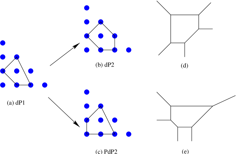
Figure 5: (a) The toric diagram of $dP1$, embedded into that of $\hbox{$\,\vrule height=6.45831pt,width=0.4pt,depth=0.0pt\kern-3.00003pt{\rm C}$}^{3}/\mathchoice{\hbox{\cmss Z\kern-3.99994ptZ}}{\hbox{\cmss Z\kern-3.99994ptZ}}{\lower 0.9pt\hbox{\cmsss Z\kern-2.79996ptZ}}{\lower 1.2pt\hbox{\cmsss Z\kern-2.79996ptZ}}_{3}\times\mathchoice{\hbox{\cmss Z\kern-3.99994ptZ}}{\hbox{\cmss Z\kern-3.99994ptZ}}{\lower 0.9pt\hbox{\cmsss Z\kern-2.79996ptZ}}{\lower 1.2pt\hbox{\cmsss Z\kern-2.79996ptZ}}_{3}$. $dP1$ can be blown up in two ways (in the toric diagram this is done by the inclusion of another point) into (b) $dP2$, the cone over the second del Pezzo surface, or (c) $PdP2$, the cone over the second pseudo del Pezzo surface. The toric $(p,q)$-web diagrams are drawn respectively in (d) and (e).

The corresponding $(p,q)$-web diagrams are given respectively in parts (d) and (e) of Figure 6. We remind the reader that these, in our nomenclature, are toric $(p,q)$-webs because they are obtained directly from dualising the toric diagrams. Indeed (d) and (e) differ because the respective toric diagrams differ; this is illustrative of the fact that toric data and toric $(p,q)$-web diagrams should be in one-to-one correspondence.

Now, in [18], these two $(p,q)$-web were obtained by the technique of splitting a brane. There, these two web diagrams were identified as those for the two different toric dual phases of $dP2$. We now point out that the web diagrams in fact correspond to different geometries and that it is important to distinguish toric and quiver $(p,q)$-webs. With some foresight, we note that the condition of [18] for splitting one external leg, such that the new external legs should not intersect with nearby external legs, is exactly the condition for addition of points in the toric diagram. We will return to this issue in a later section on splitting webs. We shall see that higgsing in the field theory, i.e., the combining of nearby external legs, is exactly the reverse process of deleting some nodes from the toric diagram to reach another [20]. In other words, the splitting and combining of external legs in the $(p,q)$-web language correspond naturally to embedding and deleting nodes in toric diagrams, and thus, to blowing up and down in the geometry. From this geometric point of view, it is natural that there is a one-to-one correspondence between the (toric) $(p,q)$-web and toric diagram.

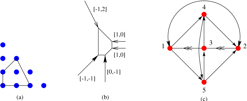
Figure 6: (a) The toric data of $PdP2$ and (b) its (toric) $(p,q)$-web diagram; these are redrawn from Figure 5. (c) the corresponding quiver diagram.

Now, let us return to the issue on bi-directional arrows and the comparison between the two webs (d) and (e) in Figure 5. The quiver diagram of $PdP2$ singularity is given in part (c) of Figure 6. Notice that this quiver diagram is exactly like phase II of $dP2$ given in the diagram in (3.4), if we ignored the bi-directional arrow between nodes 1 and 2. Once again, as in the case of $F_{2}$ and $F_{0}$ mentioned in the previous subsection, ignoring bidirectional arrows identifies two different theories. Indeed, if we calculated the quiver diagram directly from the corresponding $(p,q)$-web diagram in part (b) of Figure 6, we would have obtained phase II of $dP2$ and this is the reason why [18] identified this web as that for $dP2_{II}$. Of course, this is a vestigial feature of the fact that (2.1) does not capture bi-directional arrows. We therefore need to be careful that the “toric” $(p,q)$-web for $PdP2$ given in Part (b) of Figure 6 does not produce the right quiver for the theory but instead gives that of $dP2_{II}$.

We can further see the difference by noting that the superpotential for $PdP2$, from the Inverse Algorithm, given in terms of its 13 fields is

$$W_{PdP2} = X_{31}X_{15}X_{53}-X_{23}X_{34}X_{42}+Y_{31}X_{12}X_{23}-Y_{23}X_{31}X_{12}$$ (3.5)

$$+ X_{14}X_{42}X_{21}-X_{15}X_{52}X_{21}-Y_{31}X_{14}X_{45}X_{53}+Y_{23}X_{34}X_{45}X_{52}\ ,$$

which of course differs from $W_{dP2_{II}}$. Incidentally, we can see that this theory is invariant under the action: $1\leftrightarrow 2,4\leftrightarrow 5$ plus conjugation (i.e., reversal of arrows) of all fields (cf. [11] for discussion on these symmetries). Moreover, we can find all the toric dual phases for $PdP2$. To remain rank 1 after Seiberg duality (cf. [8] for this condition), only nodes 4 and 5 are suitable. Choosing either one (they are equivalent to each other by symmetry), we get back to the same theory. Hence, there is only one toric dual phase for $PdP2$, as opposed to $dP2$, which has two toric dual phases, as shown in (3.4)

3.3 The $PdP3$ Family of Singularities

Having seen the examples of $F_{0}$ versus $F_{2}$ and $dP2_{II}$ versus $PdP2$, let us move on. Now, starting from the toric diagram of $dP2$, we can embed it into three different toric diagrams by adding one more node. This is given in Figure 7. The first is our familiar cone over the third del Pezzo surface $dP3$ (cf. Figure 4 of [7]). The other two, in the convention above, are also what we call pseudo del Pezzo’s; these we respectively call $PdP3b$ and $PdP3c$. We have also drawn their corresponding (toric) $(p,q)$-web diagrams. We call these three members the $PdP3$ family and will address them individually. Later, as a check on the embedding of the toric data, we will demonstrate that higgsing any of $dP3$, $PdP3b$ and $PdP3c$ in the spirit of [20] gives back the $dP2$ field theory.

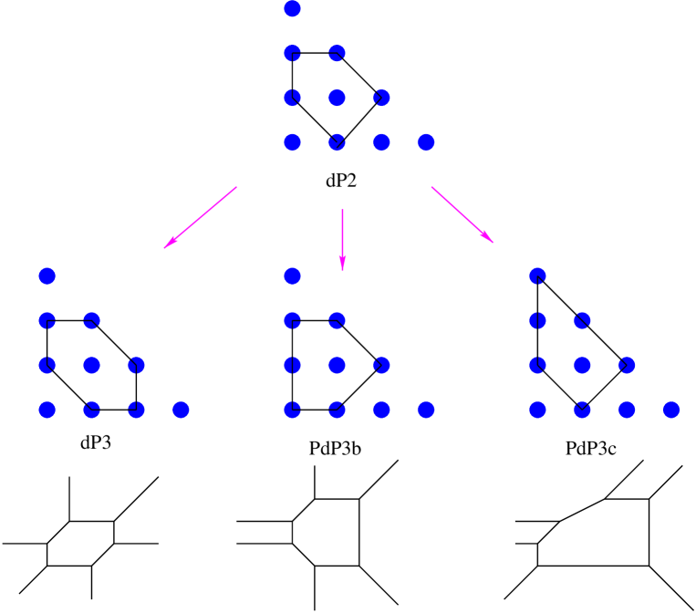
Figure 7: The possible three embeddings (unhiggsings) of $dP2$ into $dP3$, $PdP3b$ and $PdP3c$. The corresponding (toric) $(p,q)$-webs are also drawn.

3.3.1 The $PdP3b$ Singularity

Let us first analyse $PdP3b$. The Inverse Algorithm applied to $PdP3b$ from partial resolution of $\hbox{$\,\vrule height=6.45831pt,width=0.4pt,depth=0.0pt\kern-3.00003pt{\rm C}$}^{3}/\mathchoice{\hbox{\cmss Z\kern-3.99994ptZ}}{\hbox{\cmss Z\kern-3.99994ptZ}}{\lower 0.9pt\hbox{\cmsss Z\kern-2.79996ptZ}}{\lower 1.2pt\hbox{\cmsss Z\kern-2.79996ptZ}}_{3}\times\mathchoice{\hbox{\cmss Z\kern-3.99994ptZ}}{\hbox{\cmss Z\kern-3.99994ptZ}}{\lower 0.9pt\hbox{\cmsss Z\kern-2.79996ptZ}}{\lower 1.2pt\hbox{\cmsss Z\kern-2.79996ptZ}}_{3}$ results in three toric theories that are Seiberg (toric) dual to each other. The quiver diagrams and the superpotentials for these three dual phases are given below:

$$W_{PdP3b_{I}} = X_{61}X_{15}Y_{56}-X_{61}Y_{15}X_{56}+X_{16}X_{64}X_{41}-X_{16}X_{62}X_{21}$$

$$\quad-X_{41}X_{15}X_{54}+X_{21}Y_{15}X_{52}+Y_{35}X_{54}X_{43}-Y_{35}X_{52}X_{23}$$

$$\quad+X_{56}X_{62}X_{23}X_{35}-Y_{56}X_{64}X_{43}X_{35},$$

$$W_{PdP3b_{II}} = X_{12}X_{25}X_{54}X_{41}+X_{26}X_{64}X_{43}X_{32}-X_{25}X_{51}Y_{13}X_{32}-X_{64}X_{41}X_{13}X_{36}$$

$$\quad+Y_{13}X_{36}X_{61}+X_{13}X_{35}X_{51}-X_{61}X_{12}X_{26}-X_{43}X_{35}X_{54},$$

$$W_{PdP3b_{III}} = X_{13}X_{34}X_{41}-X_{46}X_{61}X_{14}+X_{45}X_{51}X_{14}-X_{24}X_{41}X_{12}+X_{62}X_{24}X_{46}$$ (3.6)

$$\quad-X_{35}X_{51}X_{13}+X_{23}X_{35}X_{56}X_{61}X_{12}-X_{23}X_{34}X_{45}X_{56}X_{62}\ .$$

We first remark on the bi-directional arrows in comparison with the 4 phases of our familiar $dP3$ theory. We will not present those quivers here due to their similarity to the ones above and the reader is referred to Figure 9 of [11]. In summary,

$$\begin{array}[]{|c|c|}\hline\cr PdP3b&dP3\\ \hline\cr II&II\\ \hline\cr I&III\\ \hline\cr III&I\\ \hline\cr\end{array}$$ (3.7)

where we have juxtaposed the quivers of the two theories that are identical if we ignored the bi-directional arrows. We remark also that because of the bi-directional arrow in $PdP3b_{I}$, the quiver has only a $\mathchoice{\hbox{\cmss Z\kern-3.99994ptZ}}{\hbox{\cmss Z\kern-3.99994ptZ}}{\lower 0.9pt\hbox{\cmsss Z\kern-2.79996ptZ}}{\lower 1.2pt\hbox{\cmsss Z\kern-2.79996ptZ}}_{2}$ symmetry with action $2\leftrightarrow 4$ and we write the superpotential in a manner to make the symmetry manifest. The same holds for $PdP3b_{III}$; the superpotential preserves only a $\mathchoice{\hbox{\cmss Z\kern-3.99994ptZ}}{\hbox{\cmss Z\kern-3.99994ptZ}}{\lower 0.9pt\hbox{\cmsss Z\kern-2.79996ptZ}}{\lower 1.2pt\hbox{\cmsss Z\kern-2.79996ptZ}}_{2}\times\mathchoice{\hbox{\cmss Z\kern-3.99994ptZ}}{\hbox{\cmss Z\kern-3.99994ptZ}}{\lower 0.9pt\hbox{\cmsss Z\kern-2.79996ptZ}}{\lower 1.2pt\hbox{\cmsss Z\kern-2.79996ptZ}}_{2}$ subgroup of the full $D_{6}$ symmetry that is expect of the quiver for $dP3$. Indeed, recalling the symmetry argument in [11], it was shown that the $\mathchoice{\hbox{\cmss Z\kern-3.99994ptZ}}{\hbox{\cmss Z\kern-3.99994ptZ}}{\lower 0.9pt\hbox{\cmsss Z\kern-2.79996ptZ}}{\lower 1.2pt\hbox{\cmsss Z\kern-2.79996ptZ}}_{2}\times\mathchoice{\hbox{\cmss Z\kern-3.99994ptZ}}{\hbox{\cmss Z\kern-3.99994ptZ}}{\lower 0.9pt\hbox{\cmsss Z\kern-2.79996ptZ}}{\lower 1.2pt\hbox{\cmsss Z\kern-2.79996ptZ}}_{2}$ symmetry uniquely determines the superpotential of phase II of $dP3$. Now since $PdP3b_{II}$ has the same quiver diagram, we should have a different symmetry in order to distinguish it. It is easy to check that this is indeed true and the phase II has only a diagonal $\mathchoice{\hbox{\cmss Z\kern-3.99994ptZ}}{\hbox{\cmss Z\kern-3.99994ptZ}}{\lower 0.9pt\hbox{\cmsss Z\kern-2.79996ptZ}}{\lower 1.2pt\hbox{\cmsss Z\kern-2.79996ptZ}}_{2}$ symmetry with action $5\leftrightarrow 6,1\leftrightarrow 3,2\leftrightarrow 4$ plus charge conjugation. We conclude that $PdP3b$ and $dP3$ are indeed markedly different theories even though they share the same quiver $(p,q)$-webs.

3.3.2 The $PdP3c$ Singularity

Our next member of the family is $PdP3c$, onto which we now move. The toric diagram and corresponding $(p,q)$-web diagram were given in Figure 7. In this case, we have two different phases, as obtained from the Inverse Algorithm, with quivers drawn in Figure 3.8 and superpotentials given as follows:

$$W_{PdP3c_{I}} = X_{12}X_{24}X_{41}+X_{45}X_{51}X_{14}-X_{13}X_{34}X_{41}-X_{46}X_{61}X_{14}$$

$$\quad+X_{13}X_{35}X_{56}X_{61}+X_{46}X_{62}X_{23}X_{34}-X_{12}X_{23}X_{35}X_{51}-X_{45}X_{56}X_{62}X_{24},$$

$$W_{PdP3c_{II}} = X_{64}X_{42}X_{26}-X_{54}X_{42}X_{25}+X_{54}X_{43}X_{35}-X_{26}X_{61}X_{12}$$ (3.8)

$$\quad+X_{24}X_{41}X_{12}-X_{24}X_{43}X_{32}+X_{13}X_{36}X_{61}-X_{13}X_{35}X_{51}$$

$$\quad+X_{25}X_{51}Y_{13}X_{32}-X_{41}Y_{13}X_{36}X_{64}\ .$$

Again, let us compare with the phases of $dP3$. For $PdP3c_{I}$, its quiver diagram is exactly the same as the phase I of $dP3$ except for the bi-directional arrow between nodes 1 and 4. This arrow breaks the $D_{6}$ symmetry of the original $dP3$ quiver down to $\mathchoice{\hbox{\cmss Z\kern-3.99994ptZ}}{\hbox{\cmss Z\kern-3.99994ptZ}}{\lower 0.9pt\hbox{\cmsss Z\kern-2.79996ptZ}}{\lower 1.2pt\hbox{\cmsss Z\kern-2.79996ptZ}}_{2}\times\mathchoice{\hbox{\cmss Z\kern-3.99994ptZ}}{\hbox{\cmss Z\kern-3.99994ptZ}}{\lower 0.9pt\hbox{\cmsss Z\kern-2.79996ptZ}}{\lower 1.2pt\hbox{\cmsss Z\kern-2.79996ptZ}}_{2}$, where one $\mathchoice{\hbox{\cmss Z\kern-3.99994ptZ}}{\hbox{\cmss Z\kern-3.99994ptZ}}{\lower 0.9pt\hbox{\cmsss Z\kern-2.79996ptZ}}{\lower 1.2pt\hbox{\cmsss Z\kern-2.79996ptZ}}_{2}$ takes $1\leftrightarrow 4,2\leftrightarrow 5,3\leftrightarrow 6$ and the other takes $2\leftrightarrow 6,3\leftrightarrow 5$ plus charge conjugation for all fields. It is easy to see these remnant symmetries from the superpotential $W_{PdP3c_{I}}$ given in (3.8). For $PdP3c_{II}$, the quiver diagram is the same as the phase II of $dP3$ except for the bi-directional arrow between nodes 2 and 4. This theory has only a diagonal $\mathchoice{\hbox{\cmss Z\kern-3.99994ptZ}}{\hbox{\cmss Z\kern-3.99994ptZ}}{\lower 0.9pt\hbox{\cmsss Z\kern-2.79996ptZ}}{\lower 1.2pt\hbox{\cmsss Z\kern-2.79996ptZ}}_{2}$ symmetry with action $1\leftrightarrow 3,2\leftrightarrow 4,5\leftrightarrow 6$ plus conjugation.

3.3.3 The $PdP3a$ Singularity

The reader may question why we have not named a $PdP3a$ singularity. We now turn precisely to this issue. The above theories of the $PdP3$ family were obtained from blowing up $dP2$; now let us examine what happens when we blow up $PdP2$ from the toric diagram in Part (a) of Figure 6. We present all possible blowups of the $PdP2$ toric diagram that still embed into $\hbox{$\,\vrule height=6.45831pt,width=0.4pt,depth=0.0pt\kern-3.00003pt{\rm C}$}^{3}/\mathchoice{\hbox{\cmss Z\kern-3.99994ptZ}}{\hbox{\cmss Z\kern-3.99994ptZ}}{\lower 0.9pt\hbox{\cmsss Z\kern-2.79996ptZ}}{\lower 1.2pt\hbox{\cmsss Z\kern-2.79996ptZ}}_{3}\times\mathchoice{\hbox{\cmss Z\kern-3.99994ptZ}}{\hbox{\cmss Z\kern-3.99994ptZ}}{\lower 0.9pt\hbox{\cmsss Z\kern-2.79996ptZ}}{\lower 1.2pt\hbox{\cmsss Z\kern-2.79996ptZ}}_{3}$ in Figure 8.

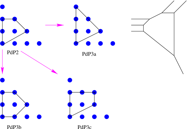
Figure 8: The three blowups of $PdP2$ into $PdP3a$, $PdP3b$ and $PdP3c$, which still embed into the parent $\hbox{$\,\vrule height=6.45831pt,width=0.4pt,depth=0.0pt\kern-3.00003pt{\rm C}$}^{3}/\mathchoice{\hbox{\cmss Z\kern-3.99994ptZ}}{\hbox{\cmss Z\kern-3.99994ptZ}}{\lower 0.9pt\hbox{\cmsss Z\kern-2.79996ptZ}}{\lower 1.2pt\hbox{\cmsss Z\kern-2.79996ptZ}}_{3}\times\mathchoice{\hbox{\cmss Z\kern-3.99994ptZ}}{\hbox{\cmss Z\kern-3.99994ptZ}}{\lower 0.9pt\hbox{\cmsss Z\kern-2.79996ptZ}}{\lower 1.2pt\hbox{\cmsss Z\kern-2.79996ptZ}}_{3}$. The toric web diagram for $PdP3a$ is also drawn. The toric $(p,q)$ webs for $PdP3b$ and $PdP3c$ are given in Figure 7.

We see that, in addition to the $PdP3b$ and $PdP3c$ obtained as blowups of $dP2$ studied in the previous subsection, we also obtain a third new singularity which we call $PdP3a$. As before, we again use the Inverse Algorithm to find the quiver and superpotential. These are given below:

$$\begin{array}[]{ll}\begin{array}[]{l}\epsfbox{PdP3a.eps}\end{array}&\begin{array}[]{rcl}&&W_{PdP3a}\\ &&=[X_{13}X_{36}X_{61}+X_{24}X_{41}X_{12}+X_{35}X_{52}X_{23}+X_{46}X_{63}X_{34}\\ &&\quad+X_{51}X_{14}X_{45}+X_{62}X_{25}X_{56}]-[X_{12}X_{25}X_{51}+X_{23}X_{36}X_{62}\\ &&\quad+X_{34}X_{41}X_{13}+X_{45}X_{52}X_{24}+X_{56}X_{63}X_{35}+X_{61}X_{14}X_{46}]\ .\end{array}\end{array}$$

There is only one toric phase for this theory. Its quiver is the same as that of model I of $dP3$ if we ignore the three bi-directional arrows connecting nodes (1,4), (2,5) and (3,6). The superpotential, written in the manner of (3.3.3), clearly manifests a $D_{6}$ symmetry: a $\mathchoice{\hbox{\cmss Z\kern-3.99994ptZ}}{\hbox{\cmss Z\kern-3.99994ptZ}}{\lower 0.9pt\hbox{\cmsss Z\kern-2.79996ptZ}}{\lower 1.2pt\hbox{\cmsss Z\kern-2.79996ptZ}}_{6}$ factor which is a $60^{o}$ degree rotation, and a $\mathchoice{\hbox{\cmss Z\kern-3.99994ptZ}}{\hbox{\cmss Z\kern-3.99994ptZ}}{\lower 0.9pt\hbox{\cmsss Z\kern-2.79996ptZ}}{\lower 1.2pt\hbox{\cmsss Z\kern-2.79996ptZ}}_{2}$ factor exchanging $2\leftrightarrow 6,3\leftrightarrow 5$ together with field conjugation.

4 Higgsing, Splitting and Blowing Up

Now we have constructed a host of theories, related to each other by blowups in the toric diagram and whose quivers can be obtained either from the toric $(p,q)$-webs or from the Inverse Algorithm. We have shown that different geometries may give rise to the same quiver if we ignored bi-directional arrows which can not be encoded into the rule (2.1) for the webs anyway. We have insisted that there is a one-one correspondence between the toric diagram and the “toric” $(p,q)$-web, which is the graph-dual of the toric diagram. On the other hand, we have introduced the notion of the “quiver” $(p,q)$-web which is simply a web that gives the right quiver by (2.1). Indeed, different geometries may have the same “quiver” $(p,q)$-web even though their “toric” $(p,q)$-webs obviously differ.

To further establish the one-to-one correspondence between the toric data and toric $(p,q)$-web diagrams, we now show that these theories above are indeed related to each other from various perspectives. This is in the spirit of the (un)higgsing mechanism of [20]. What we have used in the previous section is sequential blow-ups (blow-downs) in the toric geometry corresponding to the removal (addition) of toric points. Now we will first show that the theories can indeed be higgsed from each other from a field theory point of view. We then show that this is also in accordance with the splitting procedure in the $(p,q)$-web picture.

For example, from the toric data of $dP1$, we see that it can be embedded into both $dP2$ and $PdP2$ as shown in Figure 5. From the point of view of $(p,q)$-webs, this process is realized by splitting one external leg in the $(p,q)$-web diagram of $dP1$ [18]. To keep only one interior point in the toric data, we get only two inequivalent $(p,q)$-web diagrams by this splitting process. From the perspective of the field theory on the D-brane probe, this means that we can higgs the field theories of $dP2$ and $PdP2$ to that of $dP1$. This will be our first consistency check.

4.1 Higgsing: Checks in the Field Theory

We begin with checks from the field theory which lives on the D3-brane probe world volume. We will show that the theories obtained above by the blowups in the geometry and using the Inverse Algorithm are indeed inter-related by the higgsing mechanism.

4.1.1 From $PdP2$ to $dP1$

To higgs down from $PdP2$ to $dP1$, we start from the superpotential (3.5). By giving the field $X_{14}$ a non-zero vacuum expectation value, the fields $X_{42},X_{21}$ become massive and must be integrated out. The final theory will be left with only $13-3=10$ fields, which turns out to be precisely those of $dP1$. Indeed, after integrating out the massive fields and relabelling fields $X_{45}\rightarrow Y_{15},X_{34}\rightarrow Z_{31}$, we obtain the following superpotential:

$$W = X_{31}X_{15}X_{53}-Y_{31}Y_{15}X_{53}-X_{31}X_{12}Y_{23}+Y_{31}X_{12}X_{23}$$ (4.9)

$$\quad-X_{52}X_{23}Z_{31}X_{15}+X_{52}Y_{23}Z_{31}Y_{15}\ .$$

This is exactly the superpotential of $dP1$ given in (3.4).

4.1.2 From $PdP3b$ to $dP2$

Let us start from the phase I of $PdP3b$. First we give $X_{62}$ a non-zero VEV. In this case, fields $X_{16}$ and $X_{21}$ will become massive and should be integrated out, so we are left with $16-3=13$ fields in the final theory. After working out the superpotential as above, it is exactly that of the phase I of $dP2$ given by $W_{dP2_{I}}$ in (3.4). Next, if we give $X_{41}$ a non-zero VEV, fields $X_{16},X_{64},X_{15},X_{54}$ will get mass and we are left with $16-5=11$ fields. After integrating out the massive fields we get exactly the superpotential of phase II of $dP2$ given by $W_{dP2_{II}}$ in (3.4).

Let us now start with phase II of $PdP3b$. First, if we give field $X_{41}$ a VEV, it is easy to show that the final superpotential is exactly $W_{dP2_{I}}$. On the other hand, if we give field $X_{26}$ a non-zero VEV, we will obtain $W_{dP2_{II}}$. Recall that phase II of $PdP3b$ has the same quiver as phase II of $dP3$ and both of them can higgs down to $dP2$. Therefore, by doing the reverse procedure of unhiggsing, this gives us a non-trivial example that when we unhiggs one theory to a given quiver diagram, we may reach more than one final theory.

On the other hand, if we give $X_{25}$ the VEV, this will give the $PdP2$ theory which as we have seen has same quiver as the phase II of $dP2$ except the bi-directional arrow. Here we see a very good example how the $(p,q)$-web diagrams guide us which theory to higgs to which and where ambiguities may arises due to the bi-directional arrows. We will discuss this issue more in the next section.

4.1.3 Summary of Higgsings in the Field Theory

The calculation is thus standard and we will not present the details here for all the theories. What we will find is an intricate web of theories inter-related by the various higgsings. In the table below we present which theories, in the vertical, can be higged to which theories, in the horizontal. We explicitly indicate which fields acquire non-zero VEV’s.

$${\small\begin{array}[]{|c|c|c|c|}\hline\cr&dP2_{I}&dP2_{II}&PdP2\\ \hline\cr\hline\cr dP3_{I}&&X_{12},X_{23},X_{34},X_{45},X_{56},X_{61}&\\ \hline\cr dP3_{II}&X_{32},X_{41}&X_{25},X_{54},X_{64},X_{26}&\\ \hline\cr dP3_{III}&X_{46},X_{26}&X_{32},X_{34},X_{24},X_{12}&\\ \hline\cr dP3_{IV}&X_{51},X_{53},X_{43},X_{42},X_{52},X_{41}&&\\ \hline\cr\hline\cr PdP3a&&&X_{12},X_{23},X_{34},X_{45},X_{56},X_{61}\\ \hline\cr\hline\cr PdP3b_{I}&X_{64},X_{62}&X_{41},X_{21}&X_{43},X_{23}\\ \hline\cr PdP3b_{II}&X_{32},X_{41}&X_{26},X_{54}&X_{25},X_{64}\\ \hline\cr PdP3b_{III}&&X_{12},X_{61},X_{34},X_{45}&X_{23},X_{56}\\ \hline\cr\hline\cr PdP3c_{I}&&X_{12},X_{61},X_{34},X_{45}&X_{23},X_{56}\\ \hline\cr PdP3c_{II}&X_{32},X_{41}&X_{26},X_{54}&X_{25},X_{64}\\ \hline\cr\hline\cr\end{array}}$$ (4.10)

We remark two points. First, since the toric diagram of $dP2$ can not be embedded into that of $PdP3a$, they should not be related by higgs mechanism. This fact is shown by the empty entry in the above table. This same argument holds between $dP3$ and $PdP2$. Second, starting from phase I of $dP3$ we can never reach phase I of $dP2$ by higgsing. Conversely, $dP3_{I}$ can never be reached by the un-higgsing method of [20] applied to $dP3_{I}$. This indicates that the starting point of the un-higgsing process will effect the final result.

4.2 Splitting: Higgsing in the $(p,q)$-Web

Now, as detailed very nicely in Section 4.1 of [18], the process of (un)higgsing in the field theory, or equivalently, the process of adding/deleting nodes in the toric diagram, has a simple counterpart in the $(p,q)$-web picture. This simply corresponds to the splitting and combining of external legs (dual to the addition and deletion of points in the toric diagram). The archetypal example is given in Figure 9 below.

A strong evidence for the identification of different $(p,q)$-webs with different phases given in [18] is the ability to use the $(p,q)$-web to higgs very conveniently. The basic assumption behind this idea is the premise that the quiver diagram of a given $(p,q)$-web is calculated by the intersection number a la (2.1). As we have seen in the previous discussions, such an assumption is too strong. First, it is possible that there are bi-directional arrows in the quiver diagram. These are not captured by the intersection number which are necessarily antisymmetric. Second, when there is more than one interior point in the toric diagram, i.e., when we have parallel legs, we need more than one pair of $(p,q)$ charges to calculate the intersection. This point was shown in [10] in the mirror picture. Moreover, we will adhere to the following constraint. When we read out which fields should get a non-zero VEV from the $(p,q)$-web, we insist that only nearby external legs are combined. This condition is not required from the point of view of field theories because there are a number of fields that can develop non-zero VEVs to reach the desired result. However from the point of view of toric resolutions and indeed from the $(p,q)$-web, this condition is natural.

Bearing these points in mind, we now construct the “quiver $(p,q)$-webs” for the toric singularities studied above (incidentally, these diagrams all have only one interior point). We will reverse-engineer the $(p,q)$-charges so that the desired quiver diagrams can be calculated using (2.1) and that the various higgsings are in accordance with the conditions in the preceding paragraph. Therefore, unlike the “toric $(p,q)$-web” which is uniquely determined by graph dualisation once the toric diagram is given, for the “quiver $(p,q)$-web” we construct the web from the quiver diagram a postiori to show that the correspondence may not be one-to-one. For example, as stated earlier, the quiver $(p,q)$-web of $PdP2$ will be identical to that of phase II of $dP2$ whereas their toric $(p,q)$-webs clearly differ.

Indeed, we would like to emphasise that the toric $(p,q)$-web, obtained from the geometry alone, is perhaps a more fundamental concept. However, since the quiver $(p,q)$-web encodes the information of the quiver diagram, it can be used to efficiently encode which field gets a non-zero VEV as advocated in [18]. The $(p,q)$-webs identified with particular toric dual phases of a theory in [18] are precisely these “quiver $(p,q)$-webs.” Thus armed, let us now use a few examples to demonstrate how to use the quiver $(p,q)$-web to perform higgsing and what ambiguities may arise.

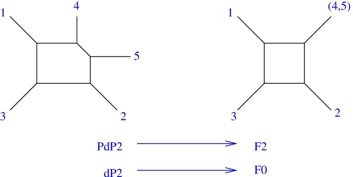
Figure 9: The higgsing of the quiver $(p,q)$-web of either $PdP2$ or $dP2_{II}$ to that of either $F_{2}$ or $F_{0}$.

4.2.1 Bi-directional Arrows

The first example is depicted in Figure 9. Since $F_{2}$ can be embedded into both $dP2$ and $PdP2$, we should expect to be able to higgs $PdP2$ and $dP2$ to $F_{2}$ as was done in the previous sections. As we have seen, the quiver diagram of $PdP2$ is same as phase II of $dP2$ up to a bi-directional arrow, so the corresponding quiver $(p,q)$-webs are same. From Figure 9 it is easy to see that by combining external legs $4$ and $5$ of left web we can get the web on the right.

According to the results in [18], this means that if we give the field $X_{45}$ a non-zero VEV, we can higgs down $PdP2$ (or $dP2$) to $F_{2}$. We have shown this, by using the explicit superpotential, in previous sections. This example demonstrates that while it is very simple to read out the higgsing information from the quiver $(p,q)$-web, the identification of field theories to a specific quiver $(p,q)$-web is ambiguous. The higgsing process dictated by a quiver $(p,q)$-web can indeed result in different field theories, depending on the theory we choose to associate with the quiver $(p,q)$-web. Thus, the same quiver $(p,q)$-webs can tell us the higgsing process of $dP2$ to $F_{0}$ or from $PdP2$ to $F_{2}$.

4.2.2 Adjacent Parallel Legs

The above ambiguities for the quiver $(p,q)$-web is by no means the whole story. The procedure to read off the higgsed fields becomes much trickier when considering $(p,q)$-webs with adjacent parallel external legs. For example, knowing the quiver diagram of phase II of $PdP3b$, we can draw its corresponding quiver $(p,q)$-web as either part (a) or (b) of Figure 10.

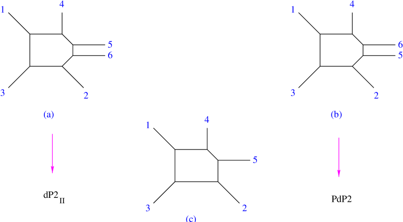
Figure 10: Higgsing the Phase II theory of $PdP3b$ down to $dP2$ or $PdP2$. Even though the latter two have the same $(p,q)$-webs, their corresponding gauge theories differ by bi-directional arrows. The different orders of label $5$ and $6$ (a) and (b) higgs down to these two different theories.

These quiver $(p,q)$-webs in Figure 10 differ from each other only by the exchange of legs $5$ and $6$ because these nodes are identical in the quiver diagram. However, when we try to higgs these two webs down to the quiver $(p,q)$-web of $dP2$ in Part (c), this difference in leg ordering becomes manifest in the higgsing procedure. Using the diagram in Part (a), by combining legs $2$ and $6$ we reach the phase II of $dP2$, but from Part (b) by combining legs $2$ and $5$ we reach $PdP2$. These are, we recall, different gauge theories.

This example demonstrates the tricky part of using quiver $(p,q)$-web in performing higgsing. In fact, this also solves the following puzzle of higgsing down from the $(p,q)$-web of $\hbox{$\,\vrule height=6.45831pt,width=0.4pt,depth=0.0pt\kern-3.00003pt{\rm C}$}^{3}/\mathchoice{\hbox{\cmss Z\kern-3.99994ptZ}}{\hbox{\cmss Z\kern-3.99994ptZ}}{\lower 0.9pt\hbox{\cmsss Z\kern-2.79996ptZ}}{\lower 1.2pt\hbox{\cmsss Z\kern-2.79996ptZ}}_{3}\times\mathchoice{\hbox{\cmss Z\kern-3.99994ptZ}}{\hbox{\cmss Z\kern-3.99994ptZ}}{\lower 0.9pt\hbox{\cmsss Z\kern-2.79996ptZ}}{\lower 1.2pt\hbox{\cmsss Z\kern-2.79996ptZ}}_{3}$. The requirement of combining only nearby legs tell us that there are four and only four different $(p,q)$-webs which we can reach from $\hbox{$\,\vrule height=6.45831pt,width=0.4pt,depth=0.0pt\kern-3.00003pt{\rm C}$}^{3}/\mathchoice{\hbox{\cmss Z\kern-3.99994ptZ}}{\hbox{\cmss Z\kern-3.99994ptZ}}{\lower 0.9pt\hbox{\cmsss Z\kern-2.79996ptZ}}{\lower 1.2pt\hbox{\cmsss Z\kern-2.79996ptZ}}_{3}\times\mathchoice{\hbox{\cmss Z\kern-3.99994ptZ}}{\hbox{\cmss Z\kern-3.99994ptZ}}{\lower 0.9pt\hbox{\cmsss Z\kern-2.79996ptZ}}{\lower 1.2pt\hbox{\cmsss Z\kern-2.79996ptZ}}_{3}$ by higgsing three fields. These are precisely the four kinds of toric singularities, viz., $dP3$, $PdP3a$, $PdP3b$ and $PdP3c$. However as we saw in §3 there are a total ten phases for $dP3$, $PdP3a$, $PdP3b$ and $PdP3c$. The answer to this puzzle is that the toric $(p,q)$-web and quiver $(p,q)$-web of $\hbox{$\,\vrule height=6.45831pt,width=0.4pt,depth=0.0pt\kern-3.00003pt{\rm C}$}^{3}/\mathchoice{\hbox{\cmss Z\kern-3.99994ptZ}}{\hbox{\cmss Z\kern-3.99994ptZ}}{\lower 0.9pt\hbox{\cmsss Z\kern-2.79996ptZ}}{\lower 1.2pt\hbox{\cmsss Z\kern-2.79996ptZ}}_{3}\times\mathchoice{\hbox{\cmss Z\kern-3.99994ptZ}}{\hbox{\cmss Z\kern-3.99994ptZ}}{\lower 0.9pt\hbox{\cmsss Z\kern-2.79996ptZ}}{\lower 1.2pt\hbox{\cmsss Z\kern-2.79996ptZ}}_{3}$ are identical but not so for the partial resolutions thereof. By switching the positions of the external leg labels in the $(p,q)$-web, we can obtain the total of ten phases of these four toric singularities. Let us now see how this is done in detail.

$A={\scriptsize\left(\matrix{0&1&0&1&0&0&0&0&1\cr 0&0&1&0&1&0&1&0&0\cr 1&0&0&0&0&1&0&1&0\cr 0&0&1&0&1&0&1&0&0\cr 1&0&0&0&0&1&0&1&0\cr 0&1&0&1&0&0&0&0&1\cr 1&0&0&0&0&1&0&1&0\cr 0&1&0&1&0&0&0&0&1\cr 0&0&1&0&1&0&1&0&0\cr}\right)},\qquad\qquad\begin{array}[]{r}\epsfbox{C3.eps}\hfil\end{array}$

Figure 11: (a) The brane box model for the matter content of $\hbox{$\,\vrule height=6.45831pt,width=0.4pt,depth=0.0pt\kern-3.00003pt{\rm C}$}^{3}/\mathchoice{\hbox{\cmss Z\kern-3.99994ptZ}}{\hbox{\cmss Z\kern-3.99994ptZ}}{\lower 0.9pt\hbox{\cmsss Z\kern-2.79996ptZ}}{\lower 1.2pt\hbox{\cmsss Z\kern-2.79996ptZ}}_{3}\times\mathchoice{\hbox{\cmss Z\kern-3.99994ptZ}}{\hbox{\cmss Z\kern-3.99994ptZ}}{\lower 0.9pt\hbox{\cmsss Z\kern-2.79996ptZ}}{\lower 1.2pt\hbox{\cmsss Z\kern-2.79996ptZ}}_{3}$ and (b) its corresponding quiver-$(p,q)$-web. Notice that we have three equivalent groups of external legs which we have labelled as $(123)$, $(456)$ and $(789)$. For every group, the order of nodes has not been specified, the $(p,q)$ charges have been written in square brackets. For reference, we have included the quiver matrix for the theory.

To start, the matter content for $\hbox{$\,\vrule height=6.45831pt,width=0.4pt,depth=0.0pt\kern-3.00003pt{\rm C}$}^{3}/\mathchoice{\hbox{\cmss Z\kern-3.99994ptZ}}{\hbox{\cmss Z\kern-3.99994ptZ}}{\lower 0.9pt\hbox{\cmsss Z\kern-2.79996ptZ}}{\lower 1.2pt\hbox{\cmsss Z\kern-2.79996ptZ}}_{3}\times\mathchoice{\hbox{\cmss Z\kern-3.99994ptZ}}{\hbox{\cmss Z\kern-3.99994ptZ}}{\lower 0.9pt\hbox{\cmsss Z\kern-2.79996ptZ}}{\lower 1.2pt\hbox{\cmsss Z\kern-2.79996ptZ}}_{3}$ is given in Part (a) of Figure 11 and the corresponding quiver $(p,q)$ is drawn in Part (b). The superpotential of the theory is:

$$W = \phi_{18}\phi_{85}\phi_{51}-\phi_{17}\phi_{75}\phi_{51}+\phi_{86}\phi_{63}\phi_{38}-\phi_{85}\phi_{53}\phi_{38}+\phi_{61}\phi_{17}\phi_{76}-\phi_{63}\phi_{37}\phi_{76}$$ (4.11)

$$+\phi_{42}\phi_{28}\phi_{84}-\phi_{41}\phi_{18}\phi_{84}+\phi_{29}\phi_{96}\phi_{62}-\phi_{28}\phi_{86}\phi_{62}+\phi_{94}\phi_{41}\phi_{19}-\phi_{96}\phi_{61}\phi_{19}$$

$$+\phi_{75}\phi_{52}\phi_{27}-\phi_{74}\phi_{42}\phi_{27}+\phi_{53}\phi_{39}\phi_{95}-\phi_{52}\phi_{29}\phi_{95}+\phi_{37}\phi_{74}\phi_{43}-\phi_{39}\phi_{94}\phi_{43}\ .$$

We now apply the higgsing mechanism to this orbifold theory to obtain all ten phases of $dP3$, $PdP3a$, $PdP3b$, and $PdP3c$.

From the corresponding toric $(p,q)$-web of $\hbox{$\,\vrule height=6.45831pt,width=0.4pt,depth=0.0pt\kern-3.00003pt{\rm C}$}^{3}/\mathchoice{\hbox{\cmss Z\kern-3.99994ptZ}}{\hbox{\cmss Z\kern-3.99994ptZ}}{\lower 0.9pt\hbox{\cmsss Z\kern-2.79996ptZ}}{\lower 1.2pt\hbox{\cmsss Z\kern-2.79996ptZ}}_{3}\times\mathchoice{\hbox{\cmss Z\kern-3.99994ptZ}}{\hbox{\cmss Z\kern-3.99994ptZ}}{\lower 0.9pt\hbox{\cmsss Z\kern-2.79996ptZ}}{\lower 1.2pt\hbox{\cmsss Z\kern-2.79996ptZ}}_{3}$ in Figure 11, we higgs down from the $U(1)^{9}$ theory down to a $U(1)^{6}$ theory by combining adjacent legs. We consequently arrive at four theories (cf. [18]):

$$\begin{array}[]{|c|c|c|}\hline\cr&&\mbox{legs combined}\\ \hline\cr(1)&dP3&[-1,0]+[1,1],\ [1,1]+[0,-1],\ [0,-1]+[-1,0]\\ \hline\cr(2)&PdP3b&[1,1]+[0,-1],\ [0,-1]+2[-1,0]\\ \hline\cr(3)&PdP3c&[0,-1]+2[1,1],\ [-1,0]+[1,1]\\ \hline\cr(4)&PdP3a&3[-1,0]+[1,1]\\ \hline\cr\end{array}$$ (4.12)

To obtain all ten theories we simply change the ordering of external legs in Part (b) of Figure 11 and hence alter the fields which obtain non-zero VEV. We summarise the relevant permutations below. The notation is such that $(a_{1}a_{2})(b_{1}b_{2})(c_{1}c_{2})$ means that the pairs of legs in each of the three brackets are to be combined.

(4.13)

In summary, the reasons that quiver $(p,q)$-web can describe more than one gauge theories are (1) it does not contain information about the bi-directions bifundamental fields; (2) the ordering ambiguities of parallel lines affects the Higgsing process. Therefore, we do not take quiver $(p,q)$-web as a fundamental concept, though it is evidently a very useful tool.

References

- [1] M. Douglas, B. Greene, and D. Morrison, “Orbifold Resolution by D-Branes”, Nucl. Phys. B506 (1997) 84-106, hep-th/9704151.
- [2] D. R. Morrison and M. R. Plesser, “Non-spherical horizons. I,” Adv. Theor. Math. Phys. 3, 1 (1999) [arXiv:hep-th/9810201].
- [3] P. S. Aspinwall, “Resolution of Orbifold Singularities in String Theory”, hep-th/9403123.
- [4] M. Douglas and G. Moore, “D-Branes, Quivers, and ALE Instantons,” hep-th/9603167.
- [5] C. Beasley, B. R. Greene, C. I. Lazaroiu, and M. R. Plesser, “D3-branes on partial resolutions of abelian quotient singularities of Calabi-Yau threefolds”, hep-th/9907186.
- [6] Duiliu-Emanuel Diaconescu, Michael R. Douglas, “D-branes on Stringy Calabi-Yau Manifolds”, hep-th/0006224.
- [7] B. Feng, A. Hanany and Y. H. He, “D-brane gauge theories from toric singularities and toric duality,” Nucl. Phys. B 595, 165 (2001) [arXiv:hep-th/0003085].
- [8] B. Feng, A. Hanany and Y. H. He, “Phase structure of D-brane gauge theories and toric duality,” JHEP 0108, 040 (2001) [arXiv:hep-th/0104259].
- [9] B. Feng, A. Hanany, Y. H. He and A. M. Uranga, “Toric duality as Seiberg duality and brane diamonds,” JHEP 0112, 035 (2001) [arXiv:hep-th/0109063].
- [10] B. Feng, A. Hanany, Y. H. He and A. Iqbal, “Quiver theories, soliton spectra and Picard-Lefschetz transformations,” arXiv:hep-th/0206152.
- [11] B. Feng, S. Franco, A. Hanany and Y. H. He, “Symmetries of toric duality,” arXiv:hep-th/0205144.
- [12] C. E. Beasley and M. R. Plesser, “Toric duality is Seiberg duality,” JHEP 0112, 001 (2001) [arXiv:hep-th/0109053].
- [13] C. E. Beasley, “Superconformal Theories from Branes at Singularities,” Unpublished Thesis.
- [14] M. Raugas, “Topics in Quantum Geometry,” Unpublished Thesis.
- [15] A. Hanany and A. Iqbal, “Quiver theories from D6-branes via mirror symmetry,” JHEP 0204, 009 (2002) [arXiv:hep-th/0108137].
- [16] F. Cachazo, B. Fiol, K. A. Intriligator, S. Katz and C. Vafa, “A geometric unification of dualities,” Nucl. Phys. B 628, 3 (2002) [arXiv:hep-th/0110028].
- [17] K. Hori, A. Iqbal, C. Vafa, “D-Branes And Mirror Symmetry”, hep-th/0005247.
- [18] S. Franco and A. Hanany, “Geometric dualities in 4d field theories and their 5d interpretation,” arXiv:hep-th/0207006.
-
[19]
S. Franco and A. Hanany,
“Toric duality, Seiberg duality and Picard-Lefschetz transformations,”
Fortsch. Phys. 51, 738 (2003)
[arXiv:hep-th/0212299].
S. Franco, A. Hanany and Y. H. He, “A trio of dualities: Walls, trees and cascades,” arXiv:hep-th/0312222. - [20] B. Feng, S. Franco, A. Hanany and Y. H. He, “Unhiggsing the del Pezzo,” arXiv:hep-th/0209228.
- [21] I. R. Klebanov and M. J. Strassler, “Supergravity and a confining gauge theory: Duality cascades and chiSB-resolution of naked singularities,” JHEP 0008, 052 (2000) [arXiv:hep-th/0007191].
-
[22]
C. P. Herzog and J. Walcher,
“Dibaryons from exceptional collections,”
JHEP 0309, 060 (2003) [arXiv:hep-th/0306298].
C. P. Herzog, “Exceptional collections and del Pezzo gauge theories,” arXiv:hep-th/0310262. -
[23]
S. Franco, A. Hanany, Y. H. He and P. Kazakopoulos,
“Duality walls, duality trees and fractional branes,”
arXiv:hep-th/0306092.
S. Franco, Y.-H. He, C. Herzog, and J. Walcher, “Chaotic Duality in String Theory,” hep-th/0402120. - [24] Y.-H. He, “On Algebraic Singularities, Finite Graphs and D-Brane Gauge Theories: A String Theoretic Perspective,” hep-th/0209230.
- [25] A. Hanany and A. M. Uranga, “Brane boxes and branes on singularities,” JHEP 9805, 013 (1998) [arXiv:hep-th/9805139].
-
[26]
S. Govindarajan and T. Jayaraman,
“D-branes, exceptional sheaves and quivers on Calabi-Yau manifolds:
From Mukai to McKay,” Nucl. Phys. B 600, 457 (2001)
[arXiv:hep-th/0010196];
A. Tomasiello, “D-branes on Calabi-Yau manifolds and helices,” JHEP 0102, 008 (2001) [arXiv:hep-th/0010217]; -
[27]
Y. H. He and J. S. Song,
“Of McKay correspondence, non-linear sigma-model and conformal field
theory,”
Adv. Theor. Math. Phys. 4, 747 (2000)
[arXiv:hep-th/9903056];
A. Hanany and Y. H. He, “Non-Abelian finite gauge theories,” JHEP 9902, 013 (1999) [arXiv:hep-th/9811183]. - [28] Martijn Wijnholt, “Large Volume Perspective on Branes at Singularities,” hep-th/0212021.
- [29] A. Hanany and E. Witten, “Type IIB superstrings, BPS monopoles, and three-dimensional gauge dynamics,” Nucl. Phys. B 492, 152 (1997) [arXiv:hep-th/9611230].
- [30] O. Aharony and A. Hanany, “Branes, superpotentials and superconformal fixed points,” Nucl. Phys. B 504, 239 (1997) [arXiv:hep-th/9704170].
- [31] O. Aharony, A. Hanany and B. Kol, “Webs of (p,q) 5-branes, five dimensional field theories and grid diagrams,” JHEP 9801, 002 (1998) [arXiv:hep-th/9710116].
- [32] N. C. Leung and C. Vafa, “Branes and toric geometry,” Adv. Theor. Math. Phys. 2, 91 (1998) [arXiv:hep-th/9711013].