Abstract

We present a matrix-model expression for the sum of instanton contributions to the prepotential of an $\mathcal{N}=2$ supersymmetric $\mathrm{U}(N)$ gauge theory, with matter in various representations. This expression is derived by combining the renormalization-group approach to the gauge theory prepotential with matrix-model methods. This result can be evaluated order-by-order in matrix-model perturbation theory to obtain the instanton corrections to the prepotential. We also show, using this expression, that the one-instanton prepotential assumes a universal form.

1 Introduction

Over the past two years, many rich connections between supersymmetric gauge theories and matrix models have been uncovered, beginning with the work of Dijkgraaf and Vafa [1, 2]. (For a review and list of references, see Ref. [3].) One aspect of this is the relation between matrix models and the Seiberg-Witten solution of $\mathcal{N}=2$ gauge theories [4], which was elucidated for gauge group $\mathrm{U}(N)$ with matter in various representations in Refs. [2, 5, 6, 7, 8, 9, 10] and for other gauge groups in Ref. [11].

In Refs. [6, 8, 9], the matrix-model approach was used to compute the one-instanton contribution to the $\mathcal{N}=2$ prepotential for $\mathrm{U}(N)$ gauge theories with matter in fundamental, symmetric, or antisymmetric representations, with the results in agreement with previous calculations made within the Seiberg-Witten framework. The matrix-model calculation requires the evaluation of the free energy to two-loops in perturbation theory (together with a tadpole calculation in the matrix model to relate the classical moduli $e_{i}$ to the quantum moduli $a_{i}$ of Seiberg-Witten theory). The final expressions for the one-instanton prepotential, however, are much simpler than the intermediate calculations. Moreover, it was observed a posteriori (in sec. 6 of Ref. [9]) that the one-instanton prepotential for all the theories considered takes the universal form

$$2\pi i\Lambda^{b_{0}}\mathcal{F}_{1-\rm inst}=\sum_{i}\frac{\langle{S_{i}}\rangle}{W_{0}^{\prime\prime}(e_{i})}+\frac{\langle{S_{0}}\rangle}{W_{0}^{\prime\prime}(m)}$$ (1.1)

where the second term is present only in theories containing an antisymmetric hypermultiplet (with mass $m$). Here $W_{0}^{\prime}(z)=\alpha\prod_{i=1}^{N}(z-e_{i})$, $\langle{S_{i}}\rangle$ and $\langle{S_{0}}\rangle$ are the values of the glueball fields $S_{i}$ and $S_{0}$ that extremize the effective superpotential, and $\Lambda^{b_{0}}$ is the one-instanton scale. Particularly intriguing is that the r.h.s. of eq. (1.1) can be evaluated using a one-loop calculation in the matrix model, despite the fact that two-loop calculations were required to arrive at this result. This strongly suggests that a much simpler route to the prepotential exists.

In this paper, we provide this simpler approach to the prepotential by combining matrix-model methods with the renormalization-group approach to the $\mathcal{N}=2$ prepotential [12, 13, 14, 15]. We obtain a general expression for the sum of the instanton contributions to the prepotential in terms of matrix-model quantities:

$$2\pi i\sum_{k=1}^{\infty}k\Lambda^{{b_{0}}k}\mathcal{F}_{k-\rm inst} = {\textstyle{1\over 2}}\sum_{i=1}^{N}\Bigg{[}\sum_{j=1}^{N}\frac{\partial}{\partial S_{j}}g_{s}\langle{{\rm tr}\,\Psi^{2}_{ii}}\rangle_{S^{2}}+\langle{{\rm tr}\,\Psi^{2}_{ii}}\rangle_{\rm disk}+4\,\langle{{\rm tr}\,\Psi^{2}_{ii}}\rangle_{\mathrm{I}\kern-1.6pt\mathrm{R}\mathrm{I}\kern-1.6pt\mathrm{P}^{2}}\Bigg{]}\Bigg{|}_{\langle{S}\rangle}$$

$$+ {\textstyle{1\over 2}}\Bigg{[}\sum_{j=1}^{N}\frac{\partial}{\partial S_{j}}g_{s}\langle{{\rm tr}\,\Psi^{2}_{00}}\rangle_{S^{2}}+\langle{{\rm tr}\,\Psi^{2}_{00}}\rangle_{\rm disk}+4\,\langle{{\rm tr}\,\Psi^{2}_{00}}\rangle_{\mathrm{I}\kern-1.6pt\mathrm{R}\mathrm{I}\kern-1.6pt\mathrm{P}^{2}}\Bigg{]}\Bigg{|}_{\langle{S}\rangle}$$

$$- {\textstyle{1\over 2}}\sum_{i=1}^{N}\Bigg{[}\sum_{j=1}^{N}\frac{\partial}{\partial S_{j}}g_{s}\langle{{\rm tr}\,\Psi_{ii}}\rangle_{S^{2}}+\langle{{\rm tr}\,\Psi_{ii}}\rangle_{\rm disk}+4\,\langle{{\rm tr}\,\Psi_{ii}}\rangle_{\mathrm{I}\kern-1.6pt\mathrm{R}\mathrm{I}\kern-1.6pt\mathrm{P}^{2}}\Bigg{]}^{2}\Bigg{|}_{\langle{S}\rangle}\,.$$

The r.h.s. can be evaluated order-by-order in matrix-model perturbation theory. The one-instanton prepotential requires only a one-loop matrix-model calculation, rather than the two-loop calculation used previously, and yields the universal expression (1.1). It is also easier to use eq. (1) to obtain higher-instanton contributions to the prepotential, as we illustrate for the case of the pure $\mathcal{N}=2$ $\mathrm{U}(N)$ theory.

Section 2 contains a review of the salient features of the Seiberg-Witten and matrix-model approaches to $\mathcal{N}=2$ supersymmetric gauge theories. Section 3 contains the main result of our paper, the derivation of eq. (1). In Sec. 4, we evaluate this expression for all $\mathrm{U}(N)$ gauge theories with asymptotically-free matter content to obtain the one-instanton correction to the prepotential. We also show that eq. (1.1) is valid for pure $\mathcal{N}=2$ $\mathrm{SO}(N)$ and $\mathrm{Sp}(N)$ theories. In Sec. 5, we compute the two-instanton prepotential for pure $\mathcal{N}=2$ $\mathrm{U}(N)$ gauge theory, using a two-loop matrix-model calculation, one loop fewer than would be required by the method of Ref. [6]. Section 6 contains our conclusions.

2 $\mathcal{N}=2$ supersymmetric gauge theory

In this section, we review $\mathcal{N}=2$ supersymmetric gauge theory, first in the Seiberg-Witten approach, and then in the matrix-model approach. Specifically, we will treat all classes of asymptotically-free $\mathcal{N}=2$ $\mathrm{SU}(N)$ gauge theories with or without matter:
(a) $\mathcal{N}=2$ $\mathrm{SU}(N)$ with $N_{f}$         hypermultiplets ($0\leq N_{f}<2N$),                
(b)  $\mathcal{N}=2$ $\mathrm{SU}(N)$ with one                 and $N_{f}$         hypermultiplets ($0\leq N_{f}<N-2$),                
(c)  $\mathcal{N}=2$ $\mathrm{SU}(N)$ with one                 and $N_{f}$         hypermultiplets ($0\leq N_{f}<N+2$),
(d) $\mathcal{N}=2$ $\mathrm{SU}(N)$ with two                 and $N_{f}$         hypermultiplets ($0\leq N_{f}<4$).

2.1 Seiberg-Witten approach

In the Seiberg-Witten (SW) approach [4], the Coulomb branch of an $\mathcal{N}=2$ gauge theory is described in terms of an algebraic curve $\Sigma$ and meromorphic differential $\lambda_{SW}$, whose explicit forms depend on the gauge group and matter content [4, 16, 17, 18]. Consider a generic point of the Coulomb branch, with the $\mathrm{SU}(N)$ gauge symmetry broken down to $\mathrm{U}(1)^{N-1}$. The SW differential can be expressed as $\lambda_{SW}=z\,T(z)\,{\rm d}z$, where

$$\oint_{A_{i}}\,T(z)\,{\rm d}z=1,\qquad\qquad\oint_{B_{i}}\,T(z)\,{\rm d}z=0$$ (2.1)

with $\{A_{i},B_{i}\}$ a canonical basis of homology cycles on $\Sigma$. The quantum moduli $a_{i}$ and their duals $a_{D,i}$ are defined as periods of the SW differential

$$a_{i}=\oint_{A_{i}}z\,T(z)\,{\rm d}z,\qquad\qquad a_{D,i}=\oint_{B_{i}}z\,T(z)\,{\rm d}z\,.$$ (2.2)

The gauge theory prepotential $\mathcal{F}(a)$ and the matrix $\tau_{ij}$ of gauge couplings of the unbroken gauge group are given by

$$a_{D,i}={\partial\mathcal{F}(a)\over{\partial a_{i}}},\qquad\qquad\tau_{ij}={\partial a_{D,i}\over\partial a_{j}}={\partial^{2}\mathcal{F}(a)\over\partial a_{i}\partial a_{j}}\,.$$ (2.3)

The SW curves and differentials for theories (a)–(d), whose explicit forms will not be needed in this paper, depend on a set of classical moduli $e_{i}$, the hypermultiplet masses, and the quantum scale $\Lambda$ of the gauge theory. By expanding $\lambda_{SW}$ in powers of $\Lambda$, one may compute the periods $a_{i}$ and $a_{D,i}$ in a weak-coupling expansion. To lowest order, $a_{i}$ coincides with the classical moduli: $a_{i}=e_{i}+\mathcal{O}(\Lambda^{b_{0}})$, where ${b_{0}}=2N-\sum_{n}I(R_{n})$ with $I(R_{n})$ the Dynkin indices of the representations $R_{n}$ of the matter hypermultiplets. Next, $a_{D,i}$ may be integrated with respect to $a_{i}$ to obtain the prepotential in the form

$$\mathcal{F}(a)=\mathcal{F}_{\rm pert}(a,\log\Lambda)+\sum_{k=1}^{\infty}\Lambda^{{b_{0}}k}\mathcal{F}_{k-\rm inst}(a)$$ (2.4)

where $\mathcal{F}_{\rm pert}(a,\log\Lambda)$ consists of the classical and one-loop prepotential, and $\mathcal{F}_{k-\rm inst}(a)$ is the $k$-instanton contribution. Using the Seiberg–Witten approach, the instanton corrections to the prepotential for theory (a) were computed in Refs. [13, 19, 20, 21]. (More recent approaches to computing the prepotential may be found in Refs. [22, 23].) For theories (b) and (c), the one-instanton prepotentials were computed in Refs. [24, 25]. For theory (d), the conjectured form of $\mathcal{F}_{1-\rm inst}$ was used in Ref. [26] to reverse-engineer the (approximate) form of the SW curve for the theory; proposals for the exact curve were made in Ref. [27], but not in a form that enabled the extraction of $\mathcal{F}_{k-\rm inst}$.

2.2 Matrix model approach

We now sketch the relation between $\mathcal{N}=2$ supersymmetric gauge theories and large $M$ matrix models, referring to Refs. [5, 6, 8, 9] for further details.

Consider an $\mathcal{N}=2$ $\mathrm{U}(N)$ gauge theory containing an $\mathcal{N}=2$ adjoint vector multiplet (which includes an $\mathcal{N}=1$ chiral superfield $\phi$) as well as $\mathcal{N}=2$ matter hypermultiplets in various representations (each of which comprises a pair of $\mathcal{N}=1$ chiral superfields $q$ and $\tilde{q}$). The superpotential for the gauge theory is taken to be $W_{0}(\phi)+W_{\mathcal{N}=2}(\phi,q,\tilde{q})$, where $W_{\mathcal{N}=2}(\phi,q,\tilde{q})$ is the $\mathcal{N}=2$ superpotential (including possible mass terms for the matter hypermultiplets) and $W_{0}^{\prime}(z)=\alpha\prod_{i=1}^{N}(z-e_{i})$. The inclusion of $W_{0}(\phi)$ in the superpotential breaks the supersymmetry to $\mathcal{N}=1$, and freezes the moduli of the Coulomb branch of vacua to $\langle{\phi}\rangle=\mathrm{diag}(e_{1},e_{2},\ldots,e_{N})$, breaking the $\mathrm{U}(N)$ gauge symmetry to $\mathrm{U}(1)^{N}$.

More general vacua (with $\langle{q}\rangle$,$\langle{\tilde{q}}\rangle\neq 0$) are possible when matter hypermultiplets are present. In particular, for theories with symmetric and antisymmetric representations, there are vacua which leave $\mathrm{Sp}(N_{0})$ or $\mathrm{SO}(N_{0})$ factors in the unbroken gauge group [28]. Thus, for theory (b), containing a symmetric hypermultiplet, the generic vacuum state has unbroken gauge group $\mathrm{SO}(N_{0})\times\prod\mathrm{U}(N_{i})$; for theory (c), containing an antisymmetric hypermultiplet, the generic vacuum state has unbroken gauge group $\mathrm{Sp}(N_{0})\times\prod\mathrm{U}(N_{i})$; for theory (d), containing two antisymmetric hypermultiplets, the generic vacuum state has unbroken gauge group $\mathrm{Sp}(N_{0})\times\mathrm{Sp}(N^{\prime}_{0})\times\prod\mathrm{U}(N_{i})$. On the Coulomb branch, one has $N_{i}=1$ for $i=1,\cdots,N$ and $N_{0}=N^{\prime}_{0}=0$. It turns out that the apparently trivial $\mathrm{Sp}(0)$ factors (but not the $\mathrm{SO}(0)$ factors) play an important role [29, 30, 31, 32] in the IR dynamics and in the matrix-model correspondence, as we will see below.

The $\mathrm{U}(N)$ gauge theory just described (with supersymmetry broken to $\mathcal{N}=1$) is related to a $\mathrm{U}(M)$ matrix model [1, 2] in which each $\mathcal{N}=1$ chiral superfield of the gauge theory has a matrix-model analog: specifically, an $M\times M$ matrix $\Phi$ (corresponding to $\phi$) together with $Q$ and $\tilde{Q}$, which are vectors or symmetric/antisymmetric matrices depending on the representation of the corresponding matter superfields $q$ and $\tilde{q}$. The superpotential of the gauge theory is taken to be the potential of the matrix model, whose partition function is

$$Z=\frac{1}{\mathrm{vol}(G)}\int{\rm d}\Phi\,{\rm d}Q\,{\rm d}\tilde{Q}\,\exp\left(-{1\over g_{s}}\left[W_{0}(\Phi)+W_{\mathcal{N}=2}(\Phi,Q,\tilde{Q})\right]\right)$$ (2.5)

where $G$ is the unbroken gauge group of the matrix model.

The partition function (2.5) is evaluated perturbatively about the extremum

$$\Phi_{0}=\pmatrix{m1\kern-3.0pt\mathrm{l}_{M_{0}}&0&\cdots&0\cr 0&e_{1}1\kern-3.0pt\mathrm{l}_{M_{1}}&\cdots&0\cr\vdots&\vdots&\ddots&\vdots\cr 0&0&\cdots&e_{N}1\kern-3.0pt\mathrm{l}_{M_{N}}},\qquad\qquad M=M_{0}+\sum_{i=1}^{N}M_{i}$$ (2.6)

where the $M_{0}\times M_{0}$ block (with $M_{0}$ even) is included only when the gauge theory contains an antisymmetric hypermultiplet (of mass $m$). In general, $Q$ and $\tilde{Q}$ vanish at the extremum, except when the theory contains an antisymmetric hypermultiplet, in which case $Q_{0}$ and $\tilde{Q}_{0}$ contain $M_{0}\times M_{0}$ blocks proportional to the symplectic unit $J$. When the $M_{0}\times M_{0}$ block is absent, the vacuum state (2.6) breaks the $\mathrm{U}(M)$ symmetry of the matrix model to $G=\prod_{i=1}^{N}\mathrm{U}(M_{i})$. When the $M_{0}\times M_{0}$ block is present, the vacuum state (2.6) (together with $Q_{0}$ and $\tilde{Q}_{0}$) breaks the $\mathrm{U}(M)$ symmetry of the matrix model to $G=\mathrm{Sp}(M_{0})\times\prod_{i=1}^{N}\mathrm{U}(M_{i})$.

The presence of the additional $M_{0}\times M_{0}$ block for theories containing an antisymmetric representation (c), and its absence for theories containing a symmetric representation (b), was discovered to be necessary to obtain the correct SW curve, differential, and one-instanton prepotential from the matrix model in Ref. [9]. This is an example of a more general phenomenon in which the correct IR description of the gauge theory requires [29, 30, 31, 32] the inclusion of a glueball field (in this case $S_{0}=g_{s}M_{0}$) corresponding to apparently trivial $\mathrm{Sp}(0)$ factors in the unbroken gauge group. Such a prescription resolves [30, 32] an apparent discrepancy [33, 34, 35] in a related $\mathcal{N}=1$ $\mathrm{Sp}(N)$ gauge theory.

For theories with two antisymmetric hypermultiplets (d), the unbroken gauge theory symmetry on the Coulomb branch is $\mathrm{Sp}(0)\times\mathrm{Sp}(0)\times\mathrm{U}(1)^{N}$. The prescription in Ref. [32] requires the inclusion of two glueball fields $S_{0}$ and $S^{\prime}_{0}$ for the two $\mathrm{Sp}(0)$ factors. Correspondingly, the perturbative matrix model must be expanded about an extremum that includes two additional blocks, $m1\kern-3.0pt\mathrm{l}_{M_{0}}$ and $m^{\prime}1\kern-3.0pt\mathrm{l}_{M^{\prime}_{0}}$, in $\Phi_{0}$ (and corresponding blocks, proportional to $J$, in $Q_{0}$ and $\tilde{Q}_{0}$), breaking the matrix-model symmetry to $G=\mathrm{Sp}(M_{0})\times\mathrm{Sp}(M^{\prime}_{0})\times\prod_{i=1}^{N}\mathrm{U}(M_{i})$.

To evaluate the partition function (2.5) perturbatively about eq. (2.6) we write $\Phi=\Phi_{0}+\Psi$. A gauge choice [5, 6] allows us to take $\Psi$ to be block-diagonal, $\Psi=\mathrm{diag}(\Psi_{00},\Psi_{11},\cdots,\Psi_{NN})$. The matrix-model expectation values $\langle{{\rm tr}\,\Phi^{n}}\rangle$ can also be evaluated perturbatively

$$\langle{{\rm tr}\,\Phi^{n}}\rangle=\sum_{i=1}^{N}\langle{{\rm tr}_{\rm i}\,\Phi^{n}}\rangle+\langle{{\rm tr}_{\rm 0}\,\Phi^{n}}\rangle=\sum_{i=1}^{N}\langle{{\rm tr}(e_{i}1\kern-3.0pt\mathrm{l}_{M_{i}}+\Psi_{ii})^{n}}\rangle+\langle{{\rm tr}(m1\kern-3.0pt\mathrm{l}_{M_{0}}+\Psi_{00})^{n}}\rangle$$ (2.7)

by computing matrix-model Feynman diagrams containing insertions of $\Psi^{m}_{ii}$ (and $\Psi^{m}_{00}$, for theories with an antisymmetric representation).

Alternatively, one may evaluate the partition function (2.5) using saddle-point methods (for a review, see Ref. [36]) in which case one starts from the resolvent of the matrix model

$$\omega(z)\equiv g_{s}\bigg{\langle}{\!{\rm tr}\!\left(\frac{1}{z-\Phi}\right)\!}\bigg{\rangle}=\sum_{n=0}^{\infty}z^{-n-1}g_{s}\langle{{\rm tr}\,\Phi^{n}}\rangle,\qquad\qquad g_{s}\langle{{\rm tr}\,\Phi^{n}}\rangle=\oint_{\infty}z^{n}\,\omega(z)\,{\rm d}z$$ (2.8)

where $\oint_{\infty}$ represents a large contour in the $z$-plane, taken counterclockwise. The resolvent $\omega(z)$ classically has poles at $e_{i}$ (and $m$, if an antisymmetric hypermultiplet is present). In the saddle-point approximation, these open up into cuts, and $\omega(z)$ becomes a function on a multisheeted Riemann surface. Let $A_{i}$ (and $A_{0}$) be cycles surrounding these cuts on the first sheet. The contour in eq. (2.8) may be deformed into a sum of cycles $A_{i}$, $A_{0}$, and we may identify the integral around the cut at $e_{i}$ (or $m$) with the trace over the $i$th (or $0$th) block of $\Phi$:

$$g_{s}\langle{{\rm tr}_{\rm i}\Phi^{n}}\rangle=\oint_{A_{i}}z^{n}\,\omega(z)\,{\rm d}z,\qquad\qquad g_{s}\langle{{\rm tr}_{0}\Phi^{n}}\rangle=\oint_{A_{0}}z^{n}\,\omega(z)\,{\rm d}z$$ (2.9)

of which the $n=0$ case is

$$S_{i}\equiv g_{s}M_{i}=\oint_{A_{i}}\,\omega(z)\,{\rm d}z,\qquad\qquad S_{0}\equiv g_{s}M_{0}=\oint_{A_{0}}\,\omega(z)\,{\rm d}z\,.$$ (2.10)

It follows straightforwardly from eq. (2.7) that

$$g_{s}\langle{{\rm tr}\,\Psi^{n}_{ii}}\rangle=\oint_{A_{i}}(z-e_{i})^{n}\,\omega(z)\,{\rm d}z,\qquad\qquad g_{s}\langle{{\rm tr}\,\Psi^{n}_{00}}\rangle=\oint_{A_{0}}(z-m)^{n}\,\omega(z)\,{\rm d}z$$ (2.11)

relating perturbative diagrams (with insertions of $\Psi^{n}_{ii}$ or $\Psi^{n}_{00}$) in the matrix model to certain moments of the resolvent.

The next step is to express matrix-model quantities in a large $M$ (small $g_{s}$) expansion, with $S_{i}$, $S_{0}$ fixed. The free energy can be written as

$$\log Z=\sum_{\chi\leq 2}g_{s}^{-\chi}F_{\chi}(S).$$ (2.12)

Using ’t Hooft double-line notation for the connected diagrams of the matrix model, this corresponds to the usual topological expansion [37] characterized by $\chi$, the Euler characteristic $2{-}2g{-}h{-}q$ of the surface in which the Feynman diagrams are embedded (where $g$ is the number of handles, $h$ the number of boundary components, and $q$ the number of crosscaps). In the large $M$ limit, the dominant contribution $F_{\rm s}\equiv g_{s}^{2}\log Z\big{|}_{\rm sphere}$ arises from planar diagrams that can be drawn on a sphere ($\chi=2$). Theories with fundamental representations give rise to surfaces with boundaries; the dominant boundary contribution $F_{\rm d}\equiv g_{s}\log Z\big{|}_{\rm disk}$ comes from planar diagrams on a disk ($\chi=1$). Theories with symmetric or antisymmetric representations contain nonorientable surfaces; the dominant nonorientable contribution $F_{\rm rp}\equiv g_{s}\log Z\big{|}_{\mathrm{I}\kern-1.6pt\mathrm{R}\mathrm{I}\kern-1.6pt\mathrm{P}^{2}}$ comes from planar diagrams on $\mathrm{I}\kern-2.5pt\mathrm{R}\mathrm{I}\kern-2.5pt\mathrm{P}^{2}$, a sphere with one crosscap ($\chi=1$). Hence,

$$\log Z=g_{s}^{-2}F_{\rm s}+g_{s}^{-1}\left(F_{\rm d}+F_{\rm rp}\right)+\mathcal{O}(g_{s}^{0})\,.$$ (2.13)

The resolvent can also be written in a large $M$ expansion:

$$\omega=\omega_{\rm s}+g_{s}(\omega_{\rm d}+\omega_{\rm rp})+\mathcal{O}(g_{s}^{2})\,.$$ (2.14)

The perturbative diagrams contributing to the vevs $\langle{{\rm tr}\,\Psi^{n}_{ii}}\rangle$ and $\langle{{\rm tr}\,\Psi^{n}_{00}}\rangle$ may be classified by the surface on which they can be drawn, thus

$$g_{s}\langle{{\rm tr}\,\Psi^{n}_{ii}}\rangle_{S^{2}}=\oint_{A_{i}}(z-e_{i})^{n}\,\omega_{\rm s}(z)\,{\rm d}z,\qquad g_{s}\langle{{\rm tr}\,\Psi^{n}_{00}}\rangle_{S^{2}}=\oint_{A_{0}}(z-m)^{n}\,\omega_{\rm s}(z)\,{\rm d}z,\qquad n\geq 1$$ (2.15)

and similarly for the disk and $\mathrm{I}\kern-2.5pt\mathrm{R}\mathrm{I}\kern-2.5pt\mathrm{P}^{2}$ contributions.

One last ingredient, the effective superpotential, is necessary to make the connection between the matrix model and the gauge theory. When the $\mathrm{U}(N)$ symmetry of the gauge theory is broken to $\prod_{i=1}^{N}\mathrm{U}(N_{i})$, with $N_{i}=1$, the superpotential takes the form [2, 38]

$$W_{\rm eff}=\,-\left[\sum_{j=1}^{N}\frac{\partial}{\partial S_{j}}F_{\rm s}+F_{\rm d}+4\,F_{\rm rp}\right]\,.$$ (2.16)

In the matrix model, the parameters $S_{i}$ (and $S_{0}$) are arbitrary, but extremizing (2.16) yields specific values $\langle{S_{i}}\rangle$ (and $\langle{S_{0}}\rangle$). Specializing the Riemann surface on which the resolvent (2.8) is defined to $\langle{S}\rangle$ then yields the SW curve $\Sigma$ of the gauge theory. The SW differential $\lambda_{SW}=z\,T(z)\,{\rm d}z$ is given by the matrix-model expression [8, 35, 39, 40]

$$T(z)=\Bigg{[}\sum_{j=1}^{N}\frac{\partial}{\partial S_{j}}\omega_{\rm s}+\omega_{\rm d}+4\,\omega_{\rm rp}\Bigg{]}\Bigg{|}_{\langle{S}\rangle}$$ (2.17)

also evaluated at the extrema $\langle{S}\rangle$ of the effective superpotential. Finally, for $\mathrm{U}(N)$ with (or without) fundamental hypermultiplets, the matrix of unbroken gauge couplings (2.3) is given by [2]

$$\tau_{ij}={1\over 2\pi i}\,{\partial^{2}F_{\rm s}\over\partial S_{i}\partial S_{j}}\bigg{|}_{\langle{S}\rangle}$$ (2.18)

evaluated at $\langle{S}\rangle$. The prescription for $\tau_{ij}$ is modified for theories with symmetric and antisymmetric representations [9, 40]. The $\mathcal{N}=2$ prepotential (2.3) is then obtained [6, 8, 9] by integrating $\tau_{ij}$ twice with respect to $a_{i}$.

An equivalent approach [30, 41, 42] is to define $\langle{S}\rangle$, not as the extrema of an effective superpotential, but as those values which ensure that $\,T(z)\,{\rm d}z$, defined by eq. (2.17), obeys eq. (2.1). In cases in which the unbroken gauge group contains “trivial” $\mathrm{Sp}(0)$ factors, such as the theories considered in this paper with antisymmetric hypermultiplets, one must further impose $\oint_{A_{0}}\,T(z)\,{\rm d}z=N_{0}=0$. Cachazo [30] emphasizes (in a related theory) that the vanishing of the $A_{0}$ period of $\,T(z)\,{\rm d}z$ does not imply the vanishing of $S_{0}=\oint_{A_{0}}\,\omega(z)\,{\rm d}z$. In turn, the nonvanishing of $\oint_{A_{0}}\,\omega(z)\,{\rm d}z$ implies the presence of an $M_{0}\times M_{0}$ block in $\Phi_{0}$.

3 Matrix-model computation of the ${\cal N}=2$ prepotential

In this section, we derive a new matrix-model expression for the instanton contributions to the prepotential. This simplifies the matrix-model computation of the one- and two-instanton prepotentials, and allows us to prove that $\mathcal{F}_{1-\rm inst}$ has the simple universal form (1.1) presented in the introduction.

An efficient method for computing $\mathcal{F}_{k-\rm inst}$ for the $\mathrm{SU}(N)$ gauge theory with or without fundamental representations was developed within the Seiberg-Witten approach in Refs. [13, 20] by making use of a renormalization-group equation satisfied by the $\mathcal{N}=2$ prepotential [12, 13]. This method was extended to $\mathrm{SU}(N)$ gauge theories with one symmetric or one antisymmetric representation in Refs. [14, 15], and can easily be generalized to include all cases in (b) and (c) above. In all these cases, the renormalization-group equation for the prepotential takes the form

$$2\pi i\Lambda\frac{\partial\mathcal{F}}{\partial\Lambda}={b_{0}}u_{2}+\cdots$$ (3.19)

where $\cdots$ represents moduli-independent constants, which would not affect the computation of $a_{D,i}$ or $\tau_{ij}$. Here $u_{2}$ is defined as

$$u_{2}=\oint_{\infty}{\textstyle{1\over 2}}z^{2}\,T(z)\,{\rm d}z\,.$$ (3.20)

The perturbative (one-loop) prepotential satisfies

$$2\pi i\Lambda\frac{\partial\mathcal{F}_{\rm pert}}{\partial\Lambda}={{b_{0}}\over 2}\sum_{i=1}^{N}a_{i}^{2}+\cdots$$ (3.21)

where $\cdots$ represents $a_{k}$-independent constants. (In writing this, we have assumed $\sum_{i}a_{i}=0$, as is appropriate for an $\mathrm{SU}(N)$ gauge theory.) Subtracting eq. (3.21) from (3.19), and neglecting henceforth the moduli-independent constants, we obtain

$$2\pi i\sum_{k=1}^{\infty}k\Lambda^{{b_{0}}k}\mathcal{F}_{k-\rm inst}=u_{2}+\sum_{i=1}^{N}e_{i}({\textstyle{1\over 2}}e_{i}-a_{i})-{\textstyle{1\over 2}}\sum_{i=1}^{N}(a_{i}-e_{i})^{2}$$ (3.22)

where we have introduced the classical moduli $e_{i}$. Different choices for $e_{i}$ are possible, differing at $\mathcal{O}(\Lambda^{b_{0}})$, but the prepotential $\mathcal{F}(a)$, computed using eq. (2.3), is independent of this choice [19]. Equation (3.22) is obviously valid for any choice of $e_{i}$, so we will make a convenient choice, letting $e_{i}$ be the parameters that appear naturally in the matrix-model approach (sec. 2.2).

We now use eqs. (2.1) and (2.2) to rewrite each of the terms in eq. (3.22) as a contour integral, which will be suitable for re-expressing the equation in terms of matrix-model quantities. The sheet on which eq. (3.20) is defined has cuts centered (approximately) on $z=e_{i}$. For theories containing an antisymmetric representation (of mass $m$), there is also a cut centered (approximately) on $z=m$. The contour in eq. (3.20) may be deformed to give

$$u_{2}=\sum_{i=1}^{N}\oint_{A_{i}}{\textstyle{1\over 2}}z^{2}\,T(z)\,{\rm d}z+\oint_{A_{0}}{\textstyle{1\over 2}}z^{2}\,T(z)\,{\rm d}z\,.$$ (3.23)

The first term in eq. (3.23) combines with the second term on the r.h.s. of eq. (3.22) to give

$$\sum_{i=1}^{N}\oint_{A_{i}}{\textstyle{1\over 2}}z^{2}\,T(z)\,{\rm d}z+\sum_{i=1}^{N}\oint_{A_{i}}e_{i}({\textstyle{1\over 2}}e_{i}-z)\,T(z)\,{\rm d}z=\sum_{i=1}^{N}\oint_{A_{i}}{\textstyle{1\over 2}}(z-e_{i})^{2}\,T(z)\,{\rm d}z\,.$$ (3.24)

Collecting all the contributions, we obtain

$$2\pi i\sum_{k=1}^{\infty}k\Lambda^{{b_{0}}k}\mathcal{F}_{k-\rm inst} = \mathcal{G}_{1}+\mathcal{G}_{2}+\mathcal{G}_{3}\,,$$ (3.25)

$$\mathcal{G}_{1} = \sum_{i=1}^{N}\oint_{A_{i}}{\textstyle{1\over 2}}(z-e_{i})^{2}\,T(z)\,{\rm d}z\,,$$

$$\mathcal{G}_{2} = \oint_{A_{0}}{\textstyle{1\over 2}}z^{2}\,T(z)\,{\rm d}z\,,$$

$$\mathcal{G}_{3} = -{\textstyle{1\over 2}}\sum_{i=1}^{N}\left[\oint_{A_{i}}(z-e_{i})\,T(z)\,{\rm d}z\right]^{2}$$

where $\mathcal{G}_{2}$ is present only in theories containing an antisymmetric hypermultiplet, and $\mathcal{G}_{3}$ only contributes to two-instantons and higher.

Even purely within the context of SW theory, eq. (3.25) is a useful equation for computing the instanton contributions to the prepotential by expanding $\,T(z)\,{\rm d}z$ in powers of $\Lambda$. However, our interest is in recasting this expression in terms of matrix-model quantities. Using eqs. (2.17) and (2.15) etc., we obtain

$$\mathcal{G}_{1} = {\textstyle{1\over 2}}\sum_{i=1}^{N}\Bigg{[}\sum_{j=1}^{N}\frac{\partial}{\partial S_{j}}g_{s}\langle{{\rm tr}\,\Psi^{2}_{ii}}\rangle_{S^{2}}+\langle{{\rm tr}\,\Psi^{2}_{ii}}\rangle_{\rm disk}+4\,\langle{{\rm tr}\,\Psi^{2}_{ii}}\rangle_{\mathrm{I}\kern-1.6pt\mathrm{R}\mathrm{I}\kern-1.6pt\mathrm{P}^{2}}\Bigg{]}\Bigg{|}_{\langle{S}\rangle}\,,$$

$$\mathcal{G}_{2} = {\textstyle{1\over 2}}\Bigg{[}\sum_{j=1}^{N}\frac{\partial}{\partial S_{j}}g_{s}\langle{{\rm tr}\,\Psi^{2}_{00}}\rangle_{S^{2}}+\langle{{\rm tr}\,\Psi^{2}_{00}}\rangle_{\rm disk}+4\,\langle{{\rm tr}\,\Psi^{2}_{00}}\rangle_{\mathrm{I}\kern-1.6pt\mathrm{R}\mathrm{I}\kern-1.6pt\mathrm{P}^{2}}\Bigg{]}\Bigg{|}_{\langle{S}\rangle}\,,$$ (3.26)

$$\mathcal{G}_{3} = -{\textstyle{1\over 2}}\sum_{i=1}^{N}\Bigg{[}\sum_{j=1}^{N}\frac{\partial}{\partial S_{j}}g_{s}\langle{{\rm tr}\,\Psi_{ii}}\rangle_{S^{2}}+\langle{{\rm tr}\,\Psi_{ii}}\rangle_{\rm disk}+4\,\langle{{\rm tr}\,\Psi_{ii}}\rangle_{\mathrm{I}\kern-1.6pt\mathrm{R}\mathrm{I}\kern-1.6pt\mathrm{P}^{2}}\Bigg{]}^{2}\Bigg{|}_{\langle{S}\rangle}$$

which is the main result of this paper. In writing this, we have used

$$\oint_{A_{0}}{\textstyle{1\over 2}}z^{2}\,T(z)\,{\rm d}z = \oint_{A_{0}}{\textstyle{1\over 2}}m^{2}\,T(z)\,{\rm d}z$$

$$+ m\Bigg{[}\sum_{j=1}^{N}\frac{\partial}{\partial S_{j}}g_{s}\langle{{\rm tr}\,\Psi_{00}}\rangle_{S^{2}}+\langle{{\rm tr}\,\Psi_{00}}\rangle_{\rm disk}+4\,\langle{{\rm tr}\,\Psi_{00}}\rangle_{\mathrm{I}\kern-1.6pt\mathrm{R}\mathrm{I}\kern-1.6pt\mathrm{P}^{2}}\Bigg{]}\Bigg{|}_{\langle{S}\rangle}$$

$$+ {\textstyle{1\over 2}}\Bigg{[}\sum_{j=1}^{N}\frac{\partial}{\partial S_{j}}g_{s}\langle{{\rm tr}\,\Psi^{2}_{00}}\rangle_{S^{2}}+\langle{{\rm tr}\,\Psi^{2}_{00}}\rangle_{\rm disk}+4\,\langle{{\rm tr}\,\Psi^{2}_{00}}\rangle_{\mathrm{I}\kern-1.6pt\mathrm{R}\mathrm{I}\kern-1.6pt\mathrm{P}^{2}}\Bigg{]}\Bigg{|}_{\langle{S}\rangle}$$

where the first two terms on the r.h.s. vanish because $\oint_{A_{0}}\,T(z)\,{\rm d}z=0$ and $\langle{{\rm tr}\,\Psi_{00}}\rangle_{S^{2}}=\langle{{\rm tr}\,\Psi_{00}}\rangle_{\rm disk}=\langle{{\rm tr}\,\Psi_{00}}\rangle_{\mathrm{I}\kern-1.6pt\mathrm{R}\mathrm{I}\kern-1.6pt\mathrm{P}^{2}}=0$ since $\Psi_{00}\in\mathrm{Sp}(M_{0})$ [9].

In the following two sections, we will evaluate the expression (3) for asymptotically-free $\mathcal{N}=2$ $\mathrm{U}(N)$ gauge theories.

4 Universality of the one-instanton prepotential

In this section, we will demonstrate that the one-instanton contribution to the prepotential has a simple universal form for all the theories considered in this paper (and for others as well). The only terms in eq. (3) that contribute to the one-instanton prepotential are

$$2\pi i\Lambda^{b_{0}}\mathcal{F}_{1-\rm inst}={\textstyle{1\over 2}}\bigg{[}\sum_{i=1}^{N}\sum_{j=1}^{N}\frac{\partial}{\partial S_{j}}g_{s}\langle{{\rm tr}\,\Psi^{2}_{ii}}\rangle_{S^{2}}+4\,\langle{{\rm tr}\,\Psi^{2}_{00}}\rangle_{\mathrm{I}\kern-1.6pt\mathrm{R}\mathrm{I}\kern-1.6pt\mathrm{P}^{2}}\bigg{]}\bigg{|}_{\langle{S}\rangle}\,.$$ (4.28)

Figure 1: 1-loop diagrams contributing to second order in $S_{i}$ and first order in $S_{0}$.

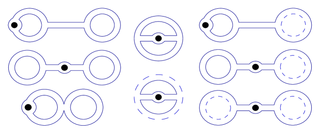
The $\mathcal{O}(S^{2})$ contribution to $\langle{{\rm tr}\,\Psi^{2}_{ii}}\rangle_{S^{2}}$ is independent of the matter content and comes from the first diagram in Fig. 1:

$$g_{s}\langle{{\rm tr}\,\Psi^{2}_{ii}}\rangle_{S^{2}}={S_{i}^{2}\over W_{0}^{\prime\prime}(e_{i})}+\mathcal{O}(S^{3}),\qquad\qquad W_{0}^{\prime\prime}(e_{i})=\alpha\prod_{j\neq i}(e_{i}-e_{j})\,.$$ (4.29)

Only theories with an antisymmetric hypermultiplet have a $\langle{{\rm tr}\,\Psi^{2}_{00}}\rangle_{\mathrm{I}\kern-1.6pt\mathrm{R}\mathrm{I}\kern-1.6pt\mathrm{P}^{2}}$ term, and the $\mathcal{O}(S)$ contribution comes from the second diagram in Fig. 1:

$$\langle{{\rm tr}\,\Psi^{2}_{00}}\rangle_{\mathrm{I}\kern-1.6pt\mathrm{R}\mathrm{I}\kern-1.6pt\mathrm{P}^{2}}=\frac{S_{0}}{2W_{0}^{\prime\prime}(m)}+\mathcal{O}(S^{2})\,.$$ (4.30)

These are the only terms contributing to the one-instanton prepotential, which becomes

$$2\pi i\Lambda^{b_{0}}\mathcal{F}_{1-\rm inst}=\sum_{i}\frac{\langle{S_{i}}\rangle}{W_{0}^{\prime\prime}(e_{i})}+\frac{\langle{S_{0}}\rangle}{W_{0}^{\prime\prime}(m)}$$ (4.31)

where the second term is only present in theories with one antisymmetric hypermultiplet (see below for theories with two antisymmetric hypermultiplets). Only the $\mathcal{O}(\Lambda^{b_{0}})$ contributions to $\langle{S_{i}}\rangle$ and $\langle{S_{0}}\rangle$ are retained in eq. (4.31), and we may replace $e_{i}$ with $a_{i}$ since the difference between these is higher order in $\Lambda$.

The fact that the one-instanton prepotential takes the universal form (4.31) was observed empirically in sec. 6 of ref. [9] for a subset of the theories considered in this paper. (This universality of form of the one-instanton prepotential was previously recognized in Refs. [26, 43] based in calculations in SW theory.)

While the form (4.31) is universal, the specific expressions for $\mathcal{F}_{1-\rm inst}$ (as functions of $a_{i}$) differ among the theories because the extrema $\langle{S_{i}}\rangle$ (and $\langle{S_{0}}\rangle$, if present) of $W_{\rm eff}$ depend on the matter content. We now evaluate (4.31) explicitly for the four classes of asymptotically-free $\mathrm{U}(N)$ theories listed at the beginning of sec. 2, as well as for pure $\mathcal{N}=2$ $\mathrm{SO}(N)$ and $\mathrm{Sp}(N)$ gauge theory.

(a) $\mathrm{U}(N)$ with $N_{f}$         hypermultiplets ($0\leq N_{f}<2N$)

To lowest order in $\Lambda$, we have [8]

$$\langle{S_{i}}\rangle={\alpha\prod_{I=1}^{N_{f}}(e_{i}+m_{I})\over R_{i}}\Lambda^{2N-N_{f}}+\cdots,\qquad\qquad R_{i}={W_{0}^{\prime\prime}(e_{i})\over\alpha}=\prod_{j\neq i}(e_{i}-e_{j})\,.$$ (4.32)

Substituting this into eq. (4.31), we obtain

$$2\pi i\mathcal{F}_{1-\rm inst}=\sum_{i}{\prod_{I=1}^{N_{f}}(a_{i}+m_{I})\over\prod_{j\neq i}(a_{i}-a_{j})^{2}}$$ (4.33)

where we have replaced $e_{i}$ by $a_{i}$, since the difference is higher order in $\Lambda$. This agrees with the expression (4.34) derived in Ref. [19] and the previous matrix-model result [8].

(b) $\mathrm{U}(N)$ with a                 hypermultiplet and $N_{f}$         hypermultiplets ($0\leq N_{f}<N-2$)

A generalization of the calculation in Ref. [9] yields

$$\langle{S_{i}}\rangle={\alpha(e_{i}-m)^{2}\prod_{j}(e_{i}+e_{j}-2m)\prod_{I=1}^{N_{f}}(e_{i}+m_{I})\over R_{i}}\Lambda^{N-2-N_{f}}+\cdots$$ (4.34)

giving the one-instanton prepotential

$$2\pi i\mathcal{F}_{1-\rm inst}=\sum_{i}{(a_{i}-m)^{2}\prod_{j}(a_{i}+a_{j}-2m)\prod_{I=1}^{N_{f}}(a_{i}+m_{I})\over\prod_{j\neq i}(a_{i}-a_{j})^{2}}$$ (4.35)

where again we have replaced $e_{i}$ with $a_{i}$. This agrees (up to a redefinition of the mass) with the one-instanton prepotential (eq. 35) obtained for this theory in Ref. [25]. This result was obtained previously using the matrix model in the $N_{f}=0$ case [9].

(c) $\mathrm{U}(N)$ with an                 hypermultiplet and $N_{f}$         hypermultiplets ($0\leq N_{f}<N+2$)

A generalization of the calculation in Ref. [9] yields

$$\langle{S_{i}}\rangle = {\alpha\prod_{j}(e_{i}+e_{j}-2m)\prod_{I=1}^{N_{f}}(e_{i}+m_{I})\over(e_{i}-m)^{2}R_{i}}\Lambda^{N+2-N_{f}}+\cdots,$$

$$\langle{S_{0}}\rangle = -\,{2W_{0}^{\prime\prime}(m)\prod_{I=1}^{N_{f}}(m+m_{I})\over\prod_{j}(e_{j}-m)}\Lambda^{N+2-N_{f}}+\cdots$$ (4.36)

which implies

$$2\pi i\mathcal{F}_{1-\rm inst}=\sum_{i}{\prod_{j}(a_{i}+a_{j}-2m)\prod_{I=1}^{N_{f}}(a_{i}+m_{I})\over(a_{i}-m)^{2}\prod_{j\neq i}(a_{i}-a_{j})^{2}}\ -\ {2\prod_{I=1}^{N_{f}}(m+m_{I})\over\prod_{j}(a_{j}-m)}$$ (4.37)

in agreement with the one-instanton prepotential (eq. 47) obtained for this theory in Ref. [25]. This result was obtained previously using the matrix model for the $N_{f}=0$ case [9].

(d) $\mathrm{U}(N)$ with two                 hypermultiplets and $N_{f}$         hypermultiplets ($0\leq N_{f}<4$)

The SW curve for this theory is known from M-theory only approximately [26, 43] or in a form [27] in which explicit calculations of the prepotential are not yet practicable, and so we cannot state with complete confidence that the renormalization group equation (3.19) holds in this case. If, however, we assume that it remains valid, the arguments of sec. 3 of this paper show that

$$2\pi i\Lambda^{b_{0}}\mathcal{F}_{1-\rm inst}=\sum_{i}\frac{\langle{S_{i}}\rangle}{W_{0}^{\prime\prime}(e_{i})}+\frac{\langle{S_{0}}\rangle}{W_{0}^{\prime\prime}(m)}+\frac{\langle{S^{\prime}_{0}}\rangle}{W_{0}^{\prime\prime}(m^{\prime})}$$ (4.38)

where, as explained in sec. 2.2, the matrix model is evaluated perturbatively about the extremum $\Phi_{0}=\mathrm{diag}(m1\kern-3.0pt\mathrm{l}_{M_{0}},m^{\prime}1\kern-3.0pt\mathrm{l}_{M^{\prime}_{0}},e_{1}1\kern-3.0pt\mathrm{l}_{M_{1}},\ldots)$. Generalizing the calculations of Ref. [9] to this case yields:

$$\langle{S_{i}}\rangle = {\alpha\prod_{j}(e_{i}+e_{j}-2m)\prod_{j}(e_{i}+e_{j}-2m^{\prime})\prod_{I=1}^{N_{f}}(e_{i}+m_{I})\over(e_{i}-m)^{2}(e_{i}-m^{\prime})^{2}R_{i}}\Lambda^{4-N_{f}}+\cdots,$$

$$\langle{S_{0}}\rangle = -{2W_{0}^{\prime\prime}(m)\prod_{j}(e_{j}+m-2m^{\prime})\prod_{I=1}^{N_{f}}(m+m_{I})\over(m-m^{\prime})^{2}\prod_{j}(e_{j}-m)}\Lambda^{4-N_{f}}+\cdots,$$ (4.39)

$$\langle{S^{\prime}_{0}}\rangle = -{2{W_{0}^{\prime\prime}(m^{\prime})}\prod_{j}(e_{j}+m^{\prime}-2m)\prod_{I=1}^{N_{f}}(m^{\prime}+m_{I})\over(m-m^{\prime})^{2}\prod_{j}(e_{j}-m^{\prime})}\Lambda^{4-N_{f}}+\cdots,$$

and thus,

$$2\pi i\mathcal{F}_{1-\rm inst}=\sum_{i}{\prod_{j}(a_{i}+a_{j}-2m)\prod_{j}(a_{i}+a_{j}-2m^{\prime})\prod_{I=1}^{N_{f}}(a_{i}+m_{I})\over(a_{i}-m)^{2}(a_{i}-m^{\prime})^{2}\prod_{j\neq i}(a_{i}-a_{j})^{2}}$$ (4.40)

$$\ -\ {2\prod_{j}(a_{j}+m-2m^{\prime})\prod_{I=1}^{N_{f}}(m+m_{I})\over(m-m^{\prime})^{2}\prod_{j}(a_{j}-m)}\ -\ {2\prod_{j}(a_{j}+m^{\prime}-2m)\prod_{I=1}^{N_{f}}(m^{\prime}+m_{I})\over(m-m^{\prime})^{2}\prod_{j}(a_{j}-m^{\prime})}$$

This is precisely what was conjectured in Ref. [26].

(e) Pure $\mathcal{N}=2$ $\mathrm{SO}(N)$ and $\mathrm{Sp}(N)$ gauge theories

Although the focus is on $\mathrm{U}(N)$ gauge theories in this paper, the expression (4.31) for the one-instanton prepotential also applies to $\mathcal{N}=2$ $\mathrm{SO}(N)$ and $\mathrm{Sp}(N)$ gauge theories [11]. For $\mathrm{SO}(N)$, there is no glueball field $S_{0}$ [32], and the leading contribution to $\langle{S_{i}}\rangle$ is

$$\langle{S_{i}}\rangle\propto\left\{\begin{array}[]{ll}(\alpha e_{i}^{4}/R_{i})\Lambda^{2N-4}&\mbox{ for even $N$},\\ (\alpha e_{i}^{2}/R_{i})\Lambda^{2N-4}&\mbox{ for odd $N$},\end{array}\right.\qquad\qquad R_{i}=\prod_{j\neq i}(e^{2}_{i}-e^{2}_{j})\,.$$ (4.41)

Substituting this into eq. (4.31), where now $W_{0}^{\prime}(z)=\alpha z\prod_{i=1}^{r}(z^{2}-e^{2}_{i})$, with $r$ the rank of the group, yields a one-instanton prepotential in agreement with Refs. [20, 21, 44].

For $\mathrm{Sp}(N)$, on the other hand, the glueball field $S_{0}$ must be included, and in fact gives the leading contribution: $\langle{S_{0}}\rangle\propto\alpha\Lambda^{N+2}$. The other vevs are subleading: $\langle{S_{i}}\rangle=\mathcal{O}(\Lambda^{2N+4})$. Substituting $\langle{S_{0}}\rangle$ into eq. (4.31), with $m=0$ and $W_{0}^{\prime}(z)=\alpha z\prod_{i=1}^{r}(z^{2}-e^{2}_{i})$, where $r=N/2$, yields a one-instanton prepotential in agreement with the Seiberg-Witten result [43]. (If massless fundamentals are present in the theory, the $\mathcal{O}(\Lambda^{N+2})$ contribution to $\langle{S_{0}}\rangle$ vanishes and the leading nonperturbative contribution to the prepotential is $\mathcal{O}(\Lambda^{2N+4})$ [20, 21, 44].)

5 Matrix-model evaluation of $\mathcal{F}_{2-\rm inst}$

In this section, we evaluate the two-instanton contribution to the prepotential for the pure $\mathcal{N}=2$ $\mathrm{U}(N)$ theory. While this computation would be quite lengthy (involving the three-loop free-energy) using the methods of Ref. [6], it is considerably simplified through the use of eqs. (3.25)–(3).

The topological expansion has no disk or $\mathrm{I}\kern-2.5pt\mathrm{R}\mathrm{I}\kern-2.5pt\mathrm{P}^{2}$ contributions, nor does $\mathcal{G}_{2}$ contribute, so eqs. (3.25)–(3). simplify to

$$2\pi i\sum_{k=1}^{\infty}k\Lambda^{2Nk}\mathcal{F}_{k-\rm inst}={\textstyle{1\over 2}}\sum_{i=1}^{N}\Bigg{[}\sum_{j=1}^{N}\frac{\partial}{\partial S_{j}}g_{s}\langle{{\rm tr}\,\Psi^{2}_{ii}}\rangle_{S^{2}}-\Bigg{(}\sum_{j=1}^{N}\frac{\partial}{\partial S_{j}}g_{s}\langle{{\rm tr}\,\Psi_{ii}}\rangle_{S^{2}}\Bigg{)}^{2}\ \Bigg{]}\Bigg{|}_{\langle{S}\rangle}\,.$$ (5.42)

Figure 2: 2-loop diagrams contributing to third order in $S$. Solid + dashed lines correspond to ghost propagators.

To evaluate the r.h.s. to two-instanton $(\mathcal{O}(\Lambda^{4N}))$ accuracy, we only require the tadpole $\langle{{\rm tr}\,\Psi_{ii}}\rangle_{S^{2}}$ to one-loop accuracy (eq. 6.1 of Ref. [6])

$$g_{s}\langle{{\rm tr}\,\Psi_{ii}}\rangle_{S^{2}}={1\over\alpha}\sum_{j\neq i}\bigg{[}-\frac{S_{i}^{2}}{R_{i}e_{ij}}+2\frac{S_{i}S_{j}}{R_{i}e_{ij}}\bigg{]}+\mathcal{O}(S^{3})$$ (5.43)

where $e_{ij}=e_{i}-e_{j}$. The $\mathcal{O}(S^{2})$ and $\mathcal{O}(S^{3})$ contributions to $\langle{{\rm tr}\,\Psi^{2}_{ii}}\rangle_{S^{2}}$ are obtained from the diagrams in Figs. 1 and 2, respectively

$$g_{s}\langle{{\rm tr}\,\Psi^{2}_{ii}}\rangle_{S^{2}} = {S_{i}^{2}\over\alpha R_{i}}+{1\over\alpha^{2}}\Bigg{[}\sum_{k\neq i}{S_{i}^{3}\over R_{i}^{2}e_{ik}^{2}}+{3S_{i}^{3}\over R_{i}^{2}}\bigg{(}\sum_{k\neq i}{1\over e_{ik}}\bigg{)}^{2}$$

$$-\sum_{k\neq i}{8S_{i}^{2}S_{k}\over R_{i}^{2}e_{ik}}\sum_{\ell\neq i}{1\over e_{i\ell}}+\sum_{k\neq i}\sum_{\ell\neq i}{4S_{i}S_{k}S_{\ell}\over R_{i}^{2}e_{ik}e_{i\ell}}-\sum_{k\neq i}{2S_{i}^{2}S_{k}\over R_{i}^{2}e_{ik}^{2}}\Bigg{]}+\mathcal{O}(S^{4})\,.$$

Substituting these expressions into eq. (5.42) gives

$$2\pi i\sum_{k=1}^{\infty}k\Lambda^{2Nk}\mathcal{F}_{k-\rm inst} = \sum_{i}{\langle{S_{i}}\rangle\over\alpha R_{i}}+{1\over\alpha^{2}}\sum_{i}\Bigg{[}{\langle{S_{i}}\rangle^{2}\over 2R_{i}^{2}}\sum_{k\neq i}{1\over e_{ik}^{2}}$$

$$+{\langle{S_{i}}\rangle^{2}\over 2R_{i}^{2}}\bigg{(}\sum_{k\neq i}{1\over e_{ik}}\bigg{)}^{2}-\sum_{k\neq i}\sum_{\ell\neq i}{4\langle{S_{i}}\rangle\langle{S_{k}}\rangle\over R_{i}^{2}e_{ik}e_{i\ell}}-\sum_{k\neq i}{2\langle{S_{i}}\rangle\langle{S_{k}}\rangle\over R_{i}^{2}e_{ik}^{2}}\Bigg{]}+\mathcal{O}(S^{3})\,.$$

The perturbative evaluation of $\langle{S_{i}}\rangle$ is given in eq. (4.17) of Ref. [6]:

$$\langle{S_{i}}\rangle={\alpha\Lambda^{2N}\over R_{i}} + {\alpha\Lambda^{4N}}\Bigg{[}\frac{1}{2R_{i}^{3}}\sum_{k\neq i}\frac{1}{e_{ik}^{2}}+\frac{2}{R_{i}^{2}}\sum_{k\neq i}\frac{1}{R_{k}e_{ik}^{2}}$$

$$+ \frac{2}{R_{i}}\sum_{k\neq i}\frac{1}{R_{k}^{2}e_{ik}^{2}}+\frac{3}{2R_{i}^{3}}\bigg{(}\sum_{k\neq i}{1\over e_{ik}}\bigg{)}^{2}+\frac{4}{R_{i}}\sum_{k\neq i}\sum_{\ell\neq k}\frac{1}{R_{k}R_{\ell}e_{ik}e_{k\ell}}\Bigg{]}+\mathcal{O}(\Lambda^{6N})\,.$$

After substituting $\langle{S_{i}}\rangle$ into eq. (5) we rewrite the expression in terms of $a_{i}$ using eq. (6.2) of Ref. [6]

$$e_{i}=a_{i}+{2\Lambda^{2N}\over R_{i}^{2}}\sum_{j\neq i}\frac{1}{a_{ij}}+\mathcal{O}(\Lambda^{4N})\,,$$ (5.47)

where $a_{ij}=a_{i}-a_{j}$, to find

$$2\pi i\sum_{k=1}^{\infty}k\Lambda^{2Nk}\mathcal{F}_{k-\rm inst} = \sum_{i}{\Lambda^{2N}\over R_{i}^{2}}+\Lambda^{4N}\sum_{i}\Bigg{[}{1\over R_{i}^{4}}\sum_{k\neq i}{1\over a_{ik}^{2}}$$

$$+{2\over R_{i}^{2}}\sum_{k\neq i}{1\over R_{k}^{2}a_{ik}^{2}}-{2\over R_{i}^{4}}\bigg{(}\sum_{k\neq i}{1\over a_{ik}}\bigg{)}^{2}+{4\over R_{i}^{2}}\sum_{k\neq i}{1\over R_{k}^{2}a_{ik}}\sum_{\ell\neq k}{1\over a_{k\ell}}$$

$$+{4\over R_{i}^{2}}\sum_{k\neq i}{1\over R_{k}a_{ik}}\sum_{\ell\neq k}{1\over R_{\ell}a_{k\ell}}-{4\over R_{i}^{3}}\sum_{k\neq i}{1\over R_{k}a_{ik}}\sum_{\ell\neq i}{1\over a_{i\ell}}\Bigg{]}+\mathcal{O}(\Lambda^{6N})$$

where here and below, $R_{i}$ is redefined as $\prod_{j\neq i}(a_{i}-a_{j})$. Finally, using identity (4.21) of Ref. [6]

$$\sum_{k\neq i}{1\over R_{k}a_{ik}}=-\ {1\over R_{i}}\sum_{k\neq i}{1\over a_{ik}}$$ (5.49)

we obtain the one- and two-instanton contributions to the prepotential for pure $\mathcal{N}=2$ $\mathrm{U}(N)$ gauge theory

$$2\pi i\mathcal{F}_{1-\rm inst} = \sum_{i}{1\over R_{i}^{2}}\,,$$

$$2\pi i\mathcal{F}_{2-\rm inst} = \sum_{i}\Bigg{[}{1\over 2R_{i}^{4}}\sum_{k\neq i}{1\over a_{ik}^{2}}+{1\over R_{i}^{2}}\sum_{k\neq i}{1\over R_{k}^{2}a_{ik}^{2}}+{1\over R_{i}^{4}}\bigg{(}\sum_{k\neq i}{1\over a_{ik}}\bigg{)}^{2}\Bigg{]}\,.$$ (5.50)

This result is precisely in agreement with eq. (4.34) in Ref. [19].

It would be straightforward to use eq. (3) to compute the two-instanton prepotential for the other theories considered in this paper.

6 Concluding remarks

Certain results of this paper deserve to be emphasized. By making use of the renormalization group equations, a general expression for the sum of the instanton contributions to the prepotential was obtained in eqs. (3.25)–(3) in terms of matrix-model quantities. The terms in eq. (3) can be computed order-by-order in matrix-model perturbation theory, simplifying the evaluation of the prepotential within this setup. In particular, a direct computation in matrix-model perturbation theory associates a $(k+1)$–loop perturbative calculation with the $k$–instanton term of the prepotential, while the method developed in this paper requires only a $k$–loop calculation to obtain the $k$–instanton prepotential. This improvement is of most practical use for low instanton number, as illustrated by our one- and two-instanton results. The exact results (3.25)–(3) may also lead to new insights into the matrix model.

On the other hand, it should be pointed out that the expression obtained in this paper is not a pure matrix-model result, as it relies on the RG equation satisfied by the prepotential, a result derived within Seiberg-Witten theory using knowledge of the SW curve and differential.

A striking result of this paper is the universal form of the one–instanton correction to the prepotential (4.31), where the dependence on the matter content appears only in the specific expressions for $\langle{S_{i}}\rangle$ and $\langle{S_{0}}\rangle$. This form applies to all aymptotically-free $\mathrm{U}(N)$ gauge theories, and to others as well (e.g., to pure $\mathcal{N}=2$ $\mathrm{SO}(N)$ and $\mathrm{Sp}(N)$ theories). In fact these regularities were previously noted in Refs. [26, 43] using the Seiberg–Witten approach to the computation of the prepotential, where the quantity $S_{i}(x)$ in Refs. [26, 43] is related to $\langle{S_{i}}\rangle$ of this paper by $S_{i}(e_{i})={\langle{S_{i}}\rangle}/W_{0}^{\prime\prime}(e_{i})$, with a similar expression for $\langle{S_{0}}\rangle$.

Appendix

In Ref. [18], the cubic curves for $\mathcal{N}=2$ $\mathrm{SU}(N)$ gauge theory with one                 (or one                 ) and $N_{f}$         hypermultiplets were derived via M-theory. In this appendix, we will transform these curves into a different set of cubic curves, which are the ones that arise in the matrix-model approach. We begin with the curve obtained in Ref. [18] for the $\mathcal{N}=2$ $\mathrm{SU}(N)$ gauge theory with one                 and $N_{f}$         hypermultiplets:

$$0 = y^{3}+\bigg{[}P(z)+{B\over z-m}+{3A\over(z-m)^{2}}\bigg{]}\,y^{2}$$

$$+{\Lambda^{{b_{0}}}j(z)\over(z-m)^{2}}\bigg{[}P(2m-z)-{B\over z-m}+{3A\over(z-m)^{2}}\bigg{]}\,y+{\Lambda^{3{b_{0}}}j(z)^{2}j(2m-z)\over(z-m)^{6}}$$

where

$$P(z)=\prod_{i=1}^{N}(z-e^{\prime}_{i}),\qquad j(z)=\prod_{I=1}^{N_{f}}(z+m_{I}),\qquad{b_{0}}=N+2-N_{f}$$ (A.2)

with $A$ and $B$ to be specified below. The classical moduli $e^{\prime}_{i}$ appearing in the curve may differ at $\mathcal{O}(\Lambda^{b_{0}})$ from the moduli $e_{i}$ used in the matrix-model approach. The curve (Appendix) lives in the space described by

$$xy=\Lambda^{2{b_{0}}}\,{j(z)j(2m-z)\over(z-m)^{4}}$$ (A.3)

modded out by the involution $x\leftrightarrow y$, $z\to 2m-z$.

To transform this curve, one first defines the variable (invariant under the involution)

$$u=\,-\,x\,-\,y\,-\,{2\Lambda^{b_{0}}j(m)\over(z-m)^{2}}\,.$$ (A.4)

Equation (A.4) may be rewritten, using (A.3), as

$$y^{2} = \,-\,uy\,-\,{2\Lambda^{b_{0}}j(m)\over(z-m)^{2}}\,\,y\,-\,{\Lambda^{2{b_{0}}}j(z)j(2m-z)\over(z-m)^{4}}\,,$$ (A.5)

$${1\over y} = \,-\,{(z-m)^{4}\over\Lambda^{2{b_{0}}}j(z)j(2m-z)}\left[u\,+\,y\,+\,{2\Lambda^{b_{0}}j(m)\over(z-m)^{2}}\right]\,.$$ (A.6)

Next divide eq. (Appendix) by $y$, and use eqs. (A.5) and (A.6) to obtain

$$y = \,-\,{\Lambda^{b_{0}}j(z)\over(z-m)^{2}}\left[u\,-\,\pi(2m-z)\over u\,-\,\pi(z)\right]\,,$$ (A.7)

$$\pi(z) \equiv P(z)\,+\,{B\over z-m}\,+\,{3A-\Lambda^{b_{0}}\left[j(z)+2j(m)\right]\over(z-m)^{2}}\,.$$ (A.8)

Substituting (A.7) into eq. (A.5), we obtain the transformed cubic curve

$$u\left[u-\pi(z)\right]\left[u-\pi(2m-z)\right]={\Lambda^{b_{0}}\over(z-m)^{2}}\Big{\{}{j(2m-z)}\,\left[u-\pi(z)\right]^{2}$$

$$\qquad+{j(z)}\,\left[u-\pi(2m-z)\right]^{2}-{2j(m)}\,\left[u-\pi(z)\right]\left[u-\pi(2m-z)\right]\Big{\}}\,.$$ (A.9)

Now, provided that the parameters $A$ and $B$ in the curve (Appendix) are given by

$$A=\Lambda^{b_{0}}j(m),\qquad B=\Lambda^{b_{0}}{{\rm d}j\over{\rm d}z}(m)$$ (A.10)

eq. (Appendix) may be written as

$$u\left[u-P(z)\right]\left[u-P(2m-z)\right]=r_{1}(z)u\,-\,t_{1}(z)$$ (A.11)

where $r_{1}(z)$ and $t_{1}(z)$ are polynomials (whose explicit forms are not particularly enlightening). Indeed, the requirement that these be polynomials was used in Ref. [18] to determine the values of $A$ and $B$. Equation (A.11) is the form of the curve that arises within the matrix-model approach to this theory [9, 28, 40].

When $\Lambda\to 0$, $r_{1}(z)$ and $t_{1}(z)$ vanish, and the curve (A.11) has singular points at the roots of $P(z)$, $P(2m-z)$, and $P(z)-P(2m-z)$. When $\Lambda\neq 0$, the curve is deformed such that the first two sets of singular points (at $z=e^{\prime}_{i}$ and $z=2m-e^{\prime}_{i}$) open up into branch cuts (on different sheets), but the singularities at the roots of $P(z)-P(2m-z)$ remain, except for the one at $z=m$, which also opens up into a branch cut. Thus, on the top sheet ($u\approx P(z)$) of the Riemann surface, there are branch cuts near $z=e^{\prime}_{i}$ and $z=m$, as was assumed in sec. 3.

The cubic curve for the $\mathcal{N}=2$ $\mathrm{SU}(N)$ gauge theory with one                 and $N_{f}$         hypermultiplets is [18]

$$0=y^{3}+P(z)\,y^{2}+{\Lambda^{{b_{0}}}(z-m)^{2}j(z)}P(2m-z)\,y+\Lambda^{3{b_{0}}}(z-m)^{6}j(z)^{2}j(2m-z)$$ (A.12)

(where now ${b_{0}}=N-2-N_{f}$) which lives in a space described by

$$xy=\Lambda^{2{b_{0}}}(z-m)^{4}j(z)j(2m-z)$$ (A.13)

modded out by the involution $x\leftrightarrow y$, $z\to 2m-z$. To transform the curve into the form obtained in the matrix model, one defines the invariant variable

$$u=\,-\,x\,-\,y\,-\,{2\Lambda^{b_{0}}j(m)\,(z-m)^{2}}$$ (A.14)

and follows the same strategy as before to obtain

$$y=\,-\,{\Lambda^{b_{0}}(z-m)^{2}j(z)}\left[u\,-\,\pi(2m-z)\over u\,-\,\pi(z)\right],\qquad\pi(z)\equiv P(z)\,-\,\Lambda^{b_{0}}(z-m)^{2}\left[j(z)+2j(m)\right]$$ (A.15)

from which one may derive the transformed cubic curve

$$u\left[u-\pi(z)\right]\left[u-\pi(2m-z)\right]={\Lambda^{b_{0}}(z-m)^{2}}\Big{\{}{j(2m-z)}\,\left[u-\pi(z)\right]^{2}$$

$$\qquad+{j(z)}\,\left[u-\pi(2m-z)\right]^{2}-{2j(m)}\,\left[u-\pi(z)\right]\left[u-\pi(2m-z)\right]\Big{\}}\,.$$ (A.16)

This may be rewritten as

$$u\left[u-P(z)+3\Lambda^{b_{0}}j(m)(z-m)^{2}\right]\left[u-P(2m-z)+3\Lambda^{b_{0}}j(m)(z-m)^{2}\right]=r_{1}(z)u\,-\,t_{1}(z)$$ (A.17)

with polynomials $r_{1}(z)$ and $t_{1}(z)$. This is the form of the curve that arises in the matrix model [9, 28, 40].

The polynomials $r_{1}(z)$ and $t_{1}(z)$ contain factors of $(z-m)^{2}$, so unlike the previous case, the singular point $z=m$ of the curve (A.17) remains present when $\Lambda\neq 0$; i.e. it does not open up into a branch cut. Thus, on the top sheet ($u\approx P(z)$) of the Riemann surface, there are branch cuts only near $z=e^{\prime}_{i}$, as was assumed in sec. 3.

References

- [1] R. Dijkgraaf and C. Vafa, Nucl. Phys. B644 (2002) 3–20, hep-th/0206255; Nucl. Phys. B644 (2002) 21–39, hep-th/0207106.
- [2] R. Dijkgraaf and C. Vafa, hep-th/0208048.
- [3] R. Argurio, G. Ferretti, and R. Heise, hep-th/0311066.
- [4] N. Seiberg and E. Witten, Nucl. Phys. B426 (1994) 19–52, hep-th/9407087; Nucl. Phys. B431 (1994) 484–550, hep-th/9408099.
- [5] R. Dijkgraaf, S. Gukov, V. A. Kazakov, and C. Vafa, Phys. Rev. D68 (2003) 045007, hep-th/0210238.
- [6] S. G. Naculich, H. J. Schnitzer, and N. Wyllard, Nucl. Phys. B651 (2003) 106–124, hep-th/0211123.
- [7] A. Klemm, M. Mariño, and S. Theisen, JHEP 03 (2003) 051, hep-th/0211216.
- [8] S. G. Naculich, H. J. Schnitzer, and N. Wyllard, JHEP 01 (2003) 015, hep-th/0211254.
- [9] S. G. Naculich, H. J. Schnitzer, and N. Wyllard, Nucl. Phys. B674 (2003) 37–79, hep-th/0305263.
-
[10]
R. Boels, J. de Boer, R. Duivenvoorden, and J. Wijnhout,
JHEP 03 (2004) 009,
hep-th/0304061;
M. Alishahiha and A. E. Mosaffa, JHEP 05 (2003) 064, hep-th/0304247;
M. Petrini, A. Tomasiello, and A. Zaffaroni, JHEP 08 (2003) 004, hep-th/0304251;
T. J. Hollowood, JHEP 10 (2003) 051, hep-th/0305023;
M. Matone and L. Mazzucato, JHEP 07 (2003) 015, hep-th/0305225. -
[11]
C.-h. Ahn and S.-k. Nam,
Phys. Rev. D67 (2003) 105022,
hep-th/0301203;
Y. Ookouchi and Y. Watabiki, Mod. Phys. Lett. A18 (2003) 1113–1126, hep-th/0301226;
R. Abbaspur, A. Imaanpur, and S. Parvizi, JHEP 07 (2003) 043, hep-th/0302083. -
[12]
M. Matone,
Phys. Lett. B357 (1995) 342–348,
hep-th/9506102;
G. Bonelli and M. Matone, Phys. Rev. Lett. 76 (1996) 4107–4110, hep-th/9602174;
G. Bonelli and M. Matone, Phys. Rev. Lett. 77 (1996) 4712–4715, hep-th/9605090;
T. Eguchi and S.-K. Yang, Mod. Phys. Lett. A11 (1996) 131–138, hep-th/9510183;
J. Sonnenschein, S. Theisen, and S. Yankielowicz, Phys. Lett. B367 (1996) 145–150, hep-th/9510129. - [13] E. D’Hoker, I. M. Krichever, and D. H. Phong, Nucl. Phys. B494 (1997) 89–104, hep-th/9610156.
- [14] E. D’Hoker, I. M. Krichever, and D. H. Phong, hep-th/0212313.
- [15] M. Gomez-Reino, JHEP 03 (2003) 043, hep-th/0301105.
[16]
A. Klemm, W. Lerche, S. Yankielowicz, and S. Theisen,
Phys. Lett. B344 (1995) 169–175,
hep-th/9411048;
P. C. Argyres and A. E. Faraggi, Phys. Rev. Lett. 74 (1995) 3931–3934, hep-th/9411057;
A. Hanany and Y. Oz, Nucl. Phys. B452 (1995) 283–312, hep-th/9505075;
P. C. Argyres, M. R. Plesser, and A. D. Shapere, Phys. Rev. Lett. 75 (1995) 1699–1702, hep-th/9505100;
J. A. Minahan and D. Nemeschansky, Nucl. Phys. B464 (1996) 3–17, hep-th/9507032;
I. M. Krichever and D. H. Phong, J. Diff. Geom. 45 (1997) 349–389, hep-th/9604199. - [17] K. Landsteiner and E. Lopez, Nucl. Phys. B516 (1998) 273–296, hep-th/9708118.
- [18] K. Landsteiner, E. Lopez, and D. A. Lowe, JHEP 07 (1998) 011, hep-th/9805158.
- [19] E. D’Hoker, I. M. Krichever, and D. H. Phong, Nucl. Phys. B489 (1997) 179–210, hep-th/9609041.
- [20] G. Chan and E. D’Hoker, Nucl. Phys. B564 (2000) 503–516, hep-th/9906193.
[21]
J. D. Edelstein, M. Mariño and J. Mas,
Nucl. Phys. B541 (1999) 671,
hep-th/9805172;
J. D. Edelstein, M. Gomez-Reino and J. Mas, Nucl. Phys. B561 (1999) 273, hep-th/9904087. -
[22]
N. A. Nekrasov,
hep-th/0206161;
hep-th/0306211;
H. Nakajima and K. Yoshioka, math.AG/0306198. -
[23]
R. Flume and R. Poghossian,
Int. J. Mod. Phys. A18 (2003) 2541,
hep-th/0208176;
U. Bruzzo, F. Fucito, J. F. Morales, and A. Tanzini, JHEP 05 (2003) 054, hep-th/0211108. -
[24]
S. G. Naculich, H. Rhedin, and H. J. Schnitzer,
Nucl. Phys. B533 (1998) 275–302,
hep-th/9804105;
I. P. Ennes, S. G. Naculich, H. Rhedin, and H. J. Schnitzer, Int. J. Mod. Phys. A14 (1999) 301–321, hep-th/9804151. - [25] I. P. Ennes, S. G. Naculich, H. Rhedin, and H. J. Schnitzer, Nucl. Phys. B536 (1998) 245–257, hep-th/9806144.
- [26] I. P. Ennes, S. G. Naculich, H. Rhedin, and H. J. Schnitzer, Nucl. Phys. B558 (1999) 41–62, hep-th/9904078.
[27]
A. E. Ksir and S. G. Naculich,
in Topics in Algebraic and Noncommutative Geometry
(Contemporary Mathematics, v. 324),
C. G. Melles et. al., eds.
(American Mathematical Society, Providence, 2003) 155–164,
hep-th/0203270;
P. C. Argyres, R. Maimon, and S. Pelland, JHEP 05 (2002) 008, hep-th/0204127. - [28] A. Klemm, K. Landsteiner, C. I. Lazaroiu, and I. Runkel, JHEP 05 (2003) 066, hep-th/0303032.
- [29] M. Aganagic, K. Intriligator, C. Vafa, and N. P. Warner, hep-th/0304271.
- [30] F. Cachazo, hep-th/0307063.
[31]
C.-h. Ahn, B. Feng, and Y. Ookouchi,
Phys. Rev. D69 (2004) 026006,
hep-th/0307190;
K. Landsteiner and C. I. Lazaroiu, hep-th/0310111. - [32] K. Intriligator, P. Kraus, A. V. Ryzhov, M. Shigemori, and C. Vafa, hep-th/0311181.
- [33] P. Kraus and M. Shigemori, JHEP 04 (2003) 052, hep-th/0303104.
- [34] L. F. Alday and M. Cirafici, JHEP 05 (2003) 041, hep-th/0304119.
- [35] P. Kraus, A. V. Ryzhov, and M. Shigemori, JHEP 05 (2003) 059, hep-th/0304138.
- [36] P. Di Francesco, P. Ginsparg, and J. Zinn-Justin, Phys. Rept. 254 (1995) 1–133, hep-th/9306153.
- [37] G. ’t Hooft, Nucl. Phys. B72 (1974) 461.
[38]
R. Argurio, V. L. Campos, G. Ferretti, and R. Heise,
Phys. Rev. D67 (2003) 065005,
hep-th/0210291;
H. Ita, H. Nieder, and Y. Oz, JHEP 01 (2003) 018, hep-th/0211261;
R. A. Janik and N. A. Obers, Phys. Lett. B553 (2003) 309–316, hep-th/0212069;
S. K. Ashok, R. Corrado, N. Halmagyi, K. D. Kennaway, and C. Romelsberger, Phys. Rev. D67 (2003) 086004, hep-th/0211291. - [39] R. Gopakumar, JHEP 05 (2003) 033, hep-th/0211100.
- [40] S. G. Naculich, H. J. Schnitzer, and N. Wyllard, JHEP 08 (2003) 021, hep-th/0303268.
- [41] F. Cachazo, N. Seiberg, and E. Witten, JHEP 04 (2003) 018, hep-th/0303207.
- [42] R. Casero and E. Trincherini, JHEP 09 (2003) 063, hep-th/0307054.
- [43] I. P. Ennes, C. Lozano, S. G. Naculich, and H. J. Schnitzer, Nucl. Phys. B576 (2000) 313–346, hep-th/9912133.
- [44] E. D’Hoker, I. M. Krichever, and D. H. Phong, Nucl. Phys. B489 (1997) 211–222, hep-th/9609145.