ANOMALOUS MAGNETIC MOMENT AND LAMB SHIFT IN THE SECOND ORDER OF THE PERTURBATION THEORY
WITH FINITE ELECTRON MASS RENORMALIZATION IN QUANTUM ELECTRODYNAMICS

Abstract

The paper determines the anomalous magnetic moment and Lamb energy level shift in the second order of the perturbation theory using the algorithm of self-energy expression regularization in quantum electrodynamics (QED) that meets the relativistic and gauge invariance requirements /1/; the comparison is made to the associated conventional quantum electrodynamics results. A limiting 4-impulse, $L^{2}=L_{0}^{2}-\vec{L}^{2}$, with an infinitely large temporal component ($\frac{L_{0}}{m}>>1)$ and limited value of spatial components $L_{i}$ that depend quite weakly on the Dirac particle impulse variation is introduced within the algorithm.

The computations in the second order of the perturbation theory result in the anomalous magnetic moment of electron, which is larger by $\sim 2.4\,$% than that in the conventional QED calculations, and the Lamb hydrogen level shift $\Delta v_{2S_{1/2}}-\Delta v_{2P_{1/2}}$, which is smaller by $\sim 6\,$ % than that in the conventional QED calculations.

The answer in regard to the agreement between the experimental data and results of the calculations by the algorithm of this paper will be given by the calculations of the next order of the perturbation theory which are being planned for the nearest future.

Merits of the algorithm suggested are:

• possibility of finite renormalization of electron and positron mass

  $$\left({m^{\left({2}\right)}=m_{0}\left({1+1.115\frac{{\alpha}}{{\pi}}}\right)}\right);$$

• agreement between the final results for the self-energy in the second order of the ”old” and relativistically covariant perturbation theory /1/;

• provision of the symmetric interaction of the electron intrinsic magnetic moment with the external magnetic and electric fields (the electron interacts both with the external magnetic field and external electric field through its intrinsic magnetic moment in the same manner in the first and second order of the perturbation theory).

1 Introduction

Ref. /1/ suggests an algorithm for regularization of the self-energy expressions for Dirac particle that meets the relativistic and gauge invariance requirements. A limiting 4-impulse, $L^{2}=L_{0}^{2}-\vec{L}^{2}$, with an infinitely large temporal component ($\frac{L_{0}}{m}>>1)$ and limited value of spatial components $L_{i}$ depending quite weakly on the particle impulse variation is introduced within the algorithm. For the particle at rest, $|\vec{L}|=m$; for the particle impulses $\frac{p}{m}$ ranging from 0 to 1, $|\vec{L}|\simeq m\left({1+0.202\frac{p^{\;4}}{m^{\;4}}-0.135\frac{p^{6}}{m^{6}}}\right)$; for the ultrarelativistic case, $|\vec{p}|>>m:|\vec{L}|\approx 2m$.

The dependence of the components $L_{i}$ on the particle impulse implies the relevant dependence on the impulse of the temporal component $L_{0}$ ensuring invariant $L^{2}=Cm^{2}$, where $C$ is a numerical coefficient much larger than one.

In the presence of external fields $A^{\mu}\left(\vec{x}\right)$ the components $L_{0}$, $L_{i}$ depend on their magnitude with the invariant $L^{2}$ remaining unchanged.

Within the algorithm suggested, in the second order of the perturbation theory the renormalized mass of Dirac particle is

$$m^{(2)}=m_{0}+\Delta m^{(2)}=m_{0}\left({1+1.115\frac{\alpha}{\pi}}\right),$$

where $m_{0}$ is the “bare” mass of the particle, $\alpha$ is the fine-structure constant.

This paper uses the algorithm /1/ to determine the anomalous magnetic moment and Lamb energy level shift in the second order of the perturbation theory. The contribution of Feynman diagrams $1a\div 1f$ presented in Fig.1 to the physical processes is calculated specifically.

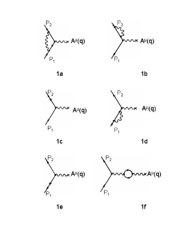
Figure 1: Electron scattering in external field $A^{\mu}(q)$. Diagrams of the second order of the perturbation theory.

In so doing the case of non-relativistic motion of charged particle $\left({|\vec{p}|<<m}\right)$ in weak external static magnetic or electric field is considered.

Like in /1/, the following computational steps are performed:

1. The integration with respect to variable $k^{0}$ (for the vertex and mass operators) or variable $p^{0}$ (for the polarization operator) is performed using the residue theorem and Feynman rule of pole bypassing.

2. The integration of impulse $k$ (for the vertex and mass operators) with respect to spatial variables is performed with introduction of the finite limit of integration $|\vec{L}|=m$.

Section 2 calculates the radiation corrections for the electron motion in a weak static homogeneous magnetic field.

Section 3 calculates the radiation corrections for the electron motion in a weak static electric field.

Section 4 summarizes the calculations and compares them to the associated results of the conventional quantum electrodynamics (QED).

2 Anomalous magnetic moment

Consider the electron motion in a weak external homogeneous magnetic field $\vec{H}$. In the final expressions we restrict our consideration only to the terms proportional to electron impulse $p_{i}$ and magnetic field $H_{i}$. Expressions proportional to $p_{i}H_{k}$ will be neglected. A contribution to the anomalous magnetic moment is made only by diagrams $1a\div 1e$.

2.1 Vertex operator

Initially consider the contribution to the anomalous magnetic moment made by the diagram $1,a$ with vertex operator $\Lambda_{\mu}^{(3)}\,(p_{1},p_{2})$. Write the process amplitude as $e\cdot\bar{u}(p_{2})\cdot\Lambda_{\mu}^{(3)}(p_{1},p_{2})\cdot A^{\mu}\cdot u(p_{1})$, where $u(p_{1})$, $\bar{u}(_{2})$ are the relevant bispinors for the initial and final state and $A^{\mu}$ is the 4-vector of the external electromagnetic field.

The vertex operator $\Lambda_{\mu}^{(3)}(p_{1},p_{2})$ can be represented as

$$\Lambda_{\mu}^{(3)}(p_{1},p_{2})=\frac{-ie^{2}}{(2\pi)^{\;4}}\int{d^{\;4}k\frac{\left({4m^{2}-2q^{2}}\right)\gamma_{\mu}-4mk_{\mu}-2\left({\hat{q}\gamma_{\mu}\hat{k}-\hat{k}\gamma_{\mu}\hat{q}}\right)-2\hat{k}\gamma_{\mu}\hat{k}}{k^{2}\left({\left({k-p_{1}}\right)^{2}-m^{2}}\right)\left({\left({k-p_{2}}\right)^{2}-m^{2}}\right)}}.$$ (1)

In (1), $q=p_{2}--p_{1}$.

When the electron moves in weak magnetic field and only those terms that are proportional to $p_{i}$ and $H_{i}$ are taken into consideration, the product $e\cdot A^{\mu}\cdot\Lambda_{\mu}^{(3)}(p_{1},p_{2})$ can be written as

$$\begin{array}[]{l}\left({-e}\right)\cdot A^{i}\cdot\Lambda^{(3)\,i}(p_{1},p_{2})=\\ {}^{=}\left({-e}\right)\frac{-ie^{2}}{(2\pi)^{\;4}}\int{d^{\;4}k\frac{B+C\cdot k_{0}+D\cdot k_{0}^{2}}{\left({k_{0}-k}\right){\kern 1.0pt}\left({k_{0}+k}\right){\kern 1.0pt}\left({k_{0}-p_{1}^{0}-\tilde{p}_{1}^{0}}\right){\kern 1.0pt}\left({k_{0}-p_{1}^{0}+\tilde{p}_{1}^{0}}\right){\kern 1.0pt}\left({k_{0}-p_{2}^{0}-\tilde{p}_{2}^{0}}\right){\kern 1.0pt}\left({k_{0}-p_{2}^{0}+\tilde{p}_{2}^{0}}\right)}}.\end{array}$$ (2)

In (2), $B=\left({4m^{2}-2k^{2}}\right)\,\vec{\gamma}{\kern 1.0pt}\vec{A}+4\left({\vec{\gamma}{\kern 1.0pt}\vec{k}}\right)\,\left({\vec{A}\cdot\vec{k}}\right)$; $C=-4\gamma^{0}\cdot\vec{\sigma}{\kern 1.0pt}\vec{H}$; $D=2\vec{\gamma}{\kern 1.0pt}\vec{A};$ $\tilde{p}_{1}^{0}=\left({m^{2}+\left({\vec{p}_{1}-\vec{k}}\right)^{2}}\right)^{1/2};\;\tilde{p}_{2}^{0}=\left({m^{2}+\left({\vec{p}_{2}-\vec{k}}\right)^{2}}\right)^{1/2}.$

Next, following the action program discussed in Introduction, integrate with respect to variable $k_{\mbox{ }}$ with using the residue theorem, for example, for the poles in the right half-plane of the complex variable $k_{0}$. Then expression (2) becomes

$$\begin{array}[]{l}\left({-e}\right)\cdot A^{i}\cdot\Lambda^{(3){\kern 1.0pt}{\kern 1.0pt}i}(p_{1},p_{2})=\\ \quad=(e)\frac{ie^{2}}{(2\pi)^{\;4}}\cdot\left({-2\pi i}\right)\int{d\vec{k}\left[{\frac{B+C\cdot k+D\cdot k^{2}}{2k\cdot\left({k-p_{1}^{0}-\tilde{p}_{1}^{0}}\right){\kern 1.0pt}\left({k-p_{1}^{0}+\tilde{p}_{1}^{0}}\right){\kern 1.0pt}\left({k-p_{2}^{0}-\tilde{p}_{2}^{0}}\right){\kern 1.0pt}\left({k-p_{2}^{0}+\tilde{p}_{2}^{0}}\right)}+}\right.}\\[7.0pt] \qquad\qquad\quad\qquad+\frac{B+C\left({p_{1}^{0}+\tilde{p}_{1}^{0}}\right)+D\left({p_{1}^{0}+\tilde{p}_{1}^{0}}\right)^{2}}{\left({\tilde{p}_{1}^{0}+p_{1}^{0}-k}\right)\;\left({\tilde{p}_{1}^{0}+p_{1}^{0}+k}\right)\cdot 2\tilde{p}_{1}^{0}\left({\tilde{p}_{1}^{0}+p_{1}^{0}-p_{2}^{0}-\tilde{p}_{2}^{0}}\right)\;\left({\tilde{p}_{1}^{0}+p_{1}^{0}-p_{2}^{0}+\tilde{p}_{2}^{0}}\right)}+\\[7.0pt] \qquad\qquad\quad\qquad+\left.{\frac{B+C\left({p_{2}^{0}+\tilde{p}_{2}^{0}}\right)+D\left({p_{2}^{0}+\tilde{p}_{2}^{0}}\right)^{2}}{\left({\tilde{p}_{2}^{0}+p_{2}^{0}-k}\right)\;\left({\tilde{p}_{2}^{0}+p_{2}^{0}+k}\right)\cdot 2\tilde{p}_{2}^{0}\left({\tilde{p}_{2}^{0}+p_{2}^{0}-p_{1}^{0}-\tilde{p}_{1}^{0}}\right)\;\left({\tilde{p}_{2}^{0}+p_{2}^{0}-p_{1}^{0}+\tilde{p}_{1}^{0}}\right)}}\right].\end{array}$$ (3)

Expression $\left({\tilde{p}_{1}^{0}+p_{1}^{0}-p_{2}^{0}-\tilde{p}_{2}^{0}}\right)$ appears in the denominators of the second and third addends in (3), and it vanishes with $\vec{p}_{1},\vec{p}_{2}\to 0$. In fact, this feature is seeming, and it is removed on appropriate algebraic transformations. After that (3) can be written as

$$\begin{array}[]{l}\left({-e}\right)\cdot A^{i}\cdot\Lambda^{(3){\kern 1.0pt}{\kern 1.0pt}i}(p_{1},p_{2})=\\[7.0pt] =(e)\frac{e^{2}}{2\cdot(2\pi)^{3}}\,\int{d\vec{k}\left\{{\frac{\left({4m^{2}-2k^{2}}\right)\,\vec{\gamma}{\kern 1.0pt}\vec{A}+4\left({\vec{\gamma}{\kern 1.0pt}\vec{k}}\right)(\vec{A}{\kern 1.0pt}\vec{k})-4\gamma^{0}\cdot\vec{\sigma}{\kern 1.0pt}\vec{H}\cdot k+2\cdot k^{2}\cdot\vec{\gamma}{\kern 1.0pt}\vec{A}}{k\left({\tilde{p}_{1}^{0}-k+p_{1}^{0}}\right)\,\left({\tilde{p}_{1}^{0}+k-p_{1}^{0}}\right)\,\left({\tilde{p}_{2}^{0}-k+p_{2}^{0}}\right)\,\left({\tilde{p}_{2}^{0}+k-p_{2}^{0}}\right)}-}\right.}\\[20.0pt] -\frac{\left[{\left({4m^{2}-2k^{2}}\right)\,\vec{\gamma}{\kern 1.0pt}\vec{A}+4\left({\vec{\gamma}{\kern 1.0pt}\vec{k}}\right)(\vec{A}{\kern 1.0pt}\vec{k})}\right]\cdot\left[{\left.{\tilde{p}_{2}^{0}\left({\left({\tilde{p}_{2}^{0}+p_{2}^{0}}\right)^{2}-k^{2}}\right)+\tilde{p}_{1}^{0}\left({\left({\tilde{p}_{1}^{0}+p_{1}^{0}}\right)^{2}-k^{2}}\right)+2\tilde{p}_{1}^{0}\cdot\tilde{p}_{2}^{0}\left({\tilde{p}_{1}^{0}+p_{1}^{0}+\tilde{p}_{2}^{0}+p_{2}^{0}}\right)}\right]}\right.}{\tilde{p}_{1}^{0}\cdot\tilde{p}_{2}^{0}\left({\tilde{p}_{1}^{0}+\tilde{p}_{2}^{0}+p_{1}^{0}-p_{2}^{0}}\right)\,\left({\tilde{p}_{2}^{0}+\tilde{p}_{1}^{0}-p_{1}^{0}+p_{2}^{0}}\right)\,\left({\left({\tilde{p}_{1}^{0}+p_{1}^{0}}\right)^{2}-k^{2}}\right)\,\left({\left({\tilde{p}_{2}^{0}+p_{2}^{0}}\right)^{2}-k^{2}}\right)}+\\[20.0pt] +\frac{4\gamma^{0}\cdot\vec{\sigma}{\kern 1.0pt}\vec{H}\left[{\tilde{p}_{2}^{0}\left({\tilde{p}_{1}^{0}+p_{1}^{0}}\right)\left({\left({\tilde{p}_{2}^{0}+p_{2}^{0}}\right)^{2}-k^{2}}\right)+\tilde{p}_{1}^{0}\left({\tilde{p}_{2}^{0}+p_{2}^{0}}\right)\left({\left({\tilde{p}_{1}^{0}+p_{1}^{0}}\right)^{2}-k^{2}}\right)+2\tilde{p}_{1}^{0}\cdot\tilde{p}_{2}^{0}\left({\left({\tilde{p}_{1}^{0}+p_{1}^{0}}\right){\kern 1.0pt}\left({\tilde{p}_{2}^{0}+p_{2}^{0}}\right)+k^{2}}\right)}\right]}{\tilde{p}_{1}^{0}\cdot\tilde{p}_{2}^{0}\left({\tilde{p}_{1}^{0}+\tilde{p}_{2}^{0}+p_{1}^{0}-p_{2}^{0}}\right){\kern 1.0pt}\left({\tilde{p}_{2}^{0}+\tilde{p}_{1}^{0}-p_{1}^{0}+p_{2}^{0}}\right){\kern 1.0pt}\left({\left({\tilde{p}_{1}^{0}+p_{1}^{0}}\right)^{2}-k^{2}}\right){\kern 1.0pt}\left({\left({\tilde{p}_{2}^{0}+p_{2}^{0}}\right)^{2}-k^{2}}\right)}-\\[20.0pt] \left.-\frac{2\vec{\gamma}{\kern 1.0pt}\vec{A}\left[{\left({\tilde{p}_{1}^{0}+p_{1}^{0}}\right)^{2}\cdot\tilde{p}_{2}^{0}\left({\left({\tilde{p}_{2}^{0}+p_{2}^{0}}\right)^{2}-k^{2}}\right)+\left({\tilde{p}_{2}^{0}+p_{2}^{0}}\right)^{2}\cdot\tilde{p}_{1}^{0}\left({\left({\tilde{p}_{1}^{0}+p_{1}^{0}}\right)^{2}-k^{2}}\right)+2\tilde{p}_{1}^{0}\cdot\tilde{p}_{2}^{0}\cdot k^{2}\left({\tilde{p}_{1}^{0}+p_{1}^{0}+\tilde{p}_{2}^{0}+p_{2}^{0}}\right)}\right]}{\tilde{p}_{1}^{0}\cdot\tilde{p}_{2}^{0}\left({\tilde{p}_{1}^{0}+\tilde{p}_{2}^{0}+p_{1}^{0}-p_{2}^{0}}\right){\kern 1.0pt}{\kern 1.0pt}\left({\tilde{p}_{2}^{0}+\tilde{p}_{1}^{0}-p_{1}^{0}+p_{2}^{0}}\right){\kern 1.0pt}{\kern 1.0pt}\left({\left({\tilde{p}_{1}^{0}+p_{1}^{0}}\right)^{2}-k^{2}}\right){\kern 1.0pt}\left({\left({\tilde{p}_{2}^{0}+p_{2}^{0}}\right)^{2}-k^{2}}\right)}\;{\kern 1.0pt}\right\}.\end{array}$$

With the accuracy degree taken by us,

$$\bar{u}\left({p_{2}}\right)\cdot\vec{\gamma}{\kern 1.0pt}\vec{A}\cdot u\left({p_{1}}\right)\simeq u\ast\left({p_{2}}\right)\left({\frac{\vec{\sigma}{\kern 1.0pt}\vec{H}}{2m}+\frac{\left({\vec{p}_{2}+\vec{p}_{1}}\right)\vec{A}}{2m}}\right)\,u\left({p_{1}}\right).$$ (4)

The contribution to the anomalous magnetic moment is seen to be made only by the first term.

In view of (4), in the integrand of (4) we can restrict our consideration only to those terms that do not depend on impulses $\vec{p}_{1},\vec{p}_{2}$. Then the integration in (4) reduces to one-dimensional integral in $k$. The integration results can be written as

$$\left({-e}\right)A^{i}\cdot\Lambda^{(3)i}(p_{1},p_{2})\!=\!(e)\frac{e^{2}}{4\pi^{2}}\frac{\vec{\sigma}\vec{H}}{4m}\!\left[{2\ln k\!-3\ln\left|{k\!+\mu}\right|\!-\frac{2}{3}\frac{k}{\mu}\!-\frac{1}{3}\frac{k\mu}{m^{2}}+\frac{1}{3}\frac{k^{2}}{m^{2}}}\right]\mathop{\left|{\begin{array}[]{l}\\ \\ \end{array}}\right.}\limits_{0}^{m}.$$ (5)

In (5), $\mu=\left({k^{2}+m^{2}}\right)^{1/2}$.

2.2 Mass operator. Mass renormalization

The contribution of the mass operator and electron mass renormalization related counterterm to the electron anomalous magnetic moment is described by diagrams $1b$, $1c$ for the electron with impulse $p_{2}$ and diagrams $1d$, $1e$ for the electron with impulse $p_{1}$. To estimate the contribution of diagrams, for example, $1b$ and $1c$, use Heitler approach /2/ and write the total process amplitude as

$$G_{3}\!=\!\frac{ie^{2}}{\left({2\pi}\right)^{\!4}}\bar{u}\left({p_{2}}\right)\left({-e}\right)\vec{\gamma}\vec{A}u\left({p_{1}}\right)\!\int\!\!{d^{\;4}k\!\frac{2m^{2}-2p_{2}\cdot k+k^{2}-\frac{2}{m^{2}}\left({p_{2}\cdot k}\right)^{2}}{\left({k^{0}\!-\!k}\right)\!\left({k^{0}\!+\!k}\right)\!\left({k^{0}\!\!-\!p_{2}^{0}-\!\tilde{p}_{2}^{0}}\right)^{2}\!\left({k^{0}\!\!-\!p_{2}^{0}\!+\!\tilde{p}_{2}^{0}}\right)^{2}}}.$$ (6)

Then integrate (6) with respect to ${\kern 1.0pt}k_{0}$, using the residue theorem with poles either in the right half-plane of complex variable ${\kern 1.0pt}k_{0}$, with the profile line closure in the lower half-plane or with poles in the left half-plane with the profile line closure in the upper half-plane. Upon the integration with respect to ${\kern 1.0pt}k_{0}$, with taking into account the accuracy degree taken by us, only the terms independent on impulse $\vec{p}_{2}$ can be left in the integrand. On the integration with respect to the solid angle and variable $k$ expression (6) can be written as

$$G_{3}=\bar{u}\left({p_{2}}\right)\,\left({-e}\right)\frac{\vec{\sigma}{\kern 1.0pt}\vec{H}}{2m}\,u\left({p_{1}}\right)\cdot\frac{e^{2}}{8\pi^{2}}\left({\ln k-\frac{3}{2}\ln\,\left|{k+\mu}\right|-\frac{k^{2}}{2m^{2}}+\frac{k\mu}{2m^{2}}}\right)\;\mathop{\left|{\begin{array}[]{l}\\ \\ \end{array}}\right.}\limits_{0}^{m}.$$ (7)

Evidently, with the accuracy degree taken, the contribution of the diagrams $1d$, $1e$ is also determined by relation (7).

In view of (5), the total contribution made by the diagrams $1a\div 1e$ to the electron anomalous magnetic moment is

$$\begin{array}[]{l}\bar{u}\left({p_{2}}\right)\frac{\alpha}{4\pi m}\,\left({-e}\right)\vec{\sigma}{\kern 1.0pt}\vec{H}\,\left({\frac{2}{3}{\kern 1.0pt}\frac{k}{\mu}-\frac{4}{3}\,\frac{k^{2}}{m^{2}}+\frac{4}{3}\,\frac{k\mu}{m^{2}}}\right)\,\mathop{\left|{\begin{array}[]{l}\\ \end{array}}\right.}\limits_{0}^{m}u\left({p_{1}}\right)=\\ =\bar{u}\left({p_{2}}\right)\frac{\alpha}{4\pi m}\left({-e}\right)\vec{\sigma}\vec{H}\left({\frac{5}{3}\sqrt{2}-\frac{4}{3}}\right)u\left({p_{1}}\right)\simeq\bar{u}\left({p_{2}}\right)\frac{\alpha}{4\pi m}1.0237\left({-e}\right)\vec{\sigma}\vec{H}\cdot u\left({p_{1}}\right).\end{array}$$ (8)

In (8), $\alpha=\frac{e^{2}}{4\pi}$ is the fine structure constant.

3 Lamb shift

In this section we consider the electron motion in weak external electric field $\vec{\varepsilon}=-\nabla A_{0}$. In the final expressions we will restrict our consideration to the terms proportional to electric field $\varepsilon_{i}$ and expansions up to the ones quadratic in electron impulse $p_{i}^{2}$. Expressions proportional to $p_{i}^{2}\varepsilon_{\kappa}$ will be neglected. The contribution to the Lamb shift is made by all diagrams $1a\div 1f$.

3.1 Vertex operator

Consider the contribution made by the diagram $1a$ with the vertex operator $\Lambda_{0}^{(3)}(p_{1},p_{2})$ to the Lamb shift. With account for the accuracy degree taken by us, product $eA_{0}\Lambda_{0}^{(3)}(p_{1},p{}_{2})$ can be written as

$$\begin{array}[]{l}eA_{0}\Lambda_{0}^{(3)}(p_{1},p_{2})=\\ =eA_{0}(-)\frac{ie^{2}}{(2\pi)^{\;4}}\int{d^{\;4}\kappa\frac{B_{1}+C_{1}\cdot k_{0}+D_{1}\cdot k_{0}^{2}}{(k_{0}-k)(k_{0}+k)(k_{0}-p_{1}^{0}-\tilde{p}_{1}^{0})(k_{0}-p_{1}^{0}+\tilde{p}_{1}^{0})(k_{0}-p_{2}^{0}-\tilde{p}_{2}^{0})(k_{0}-p_{2}^{0}+\tilde{p}_{2}^{0})}}.\end{array}$$ (9)

In (9), $B_{1}=(4m^{2}+2\vec{q}^{2}-2k^{2})\gamma_{0}+4i\gamma_{0}\vec{\sigma}(\vec{k}\times\vec{q}),$ $C_{1}=-4m+4\vec{\gamma}\,\vec{k}$, $D_{1}=$$=-2\gamma_{0}.$

Next, like in Section 2, perform the integration with respect to variable $k_{0}$ and algebraic transformations with canceling from the denominators the expression $(\tilde{p}_{1}^{0}+p_{1}^{0}-p_{2}^{0}-\tilde{p}_{2}^{0})$ that vanishes with $\vec{p}_{1},\;\vec{p}_{2}\to 0.$

As a result, expression (9) can be written as:

$$\begin{array}[]{l}eA_{0}\Lambda_{0}^{(3)}(p_{1},p_{2})\!=\!-eA_{0}\!\frac{e^{2}}{2(2\pi)^{3}}\int\!{d\vec{k}\left\{{\frac{(4m^{2}+2\vec{q}^{2}-2k^{2})\gamma_{0}-4i\gamma_{0}(\vec{\sigma}\times\vec{q})\vec{k}-4m\cdot k+4\cdot\kappa\cdot\vec{\gamma}\vec{k}-2\gamma_{0}\cdot k^{2}}{k(\tilde{p}_{1}^{0}-k+p_{1}^{0})(\tilde{p}_{1}^{0}+k-p_{1}^{0})(\tilde{p}_{2}^{0}-k+p_{2}^{0})(\tilde{p}_{2}^{0}+k-p_{2}^{0})}}\right.}-\\[14.0pt] \quad-\frac{(4m^{2}+2\vec{q}^{2}-2k^{2}-4i(\vec{\sigma}\times\vec{q})\cdot\vec{k})\cdot\gamma_{0}[\tilde{p}_{2}^{o}((\tilde{p}_{2}^{0}+p_{2}^{0})^{2}-k^{2})+\tilde{p}_{1}^{0}((\tilde{p}_{1}^{0}+p_{1}^{0})^{2}-k^{2})+2\tilde{p}_{1}\cdot\tilde{p}_{2}^{0}(\tilde{p}_{1}^{0}+p_{1}^{0}+\tilde{p}_{2}^{0}+p_{2}^{0})]}{\tilde{p}_{1}^{0}\tilde{p}_{2}^{0}(\tilde{p}_{1}^{0}+\tilde{p}_{2}^{0}+p_{1}^{0}-p_{2}^{0})(\tilde{p}_{2}^{0}+\tilde{p}_{1}^{0}-p_{1}^{0}+p_{2}^{0})((\tilde{p}_{1}^{0}+p_{1}^{0})^{2}-k^{2})((\tilde{p}_{2}^{0}+p_{2}^{0})^{2}-k^{2})}-\\[14.0pt] \quad-\frac{(-4m+4\vec{\gamma}\vec{k})[\tilde{p}_{2}^{0}(\tilde{p}_{1}^{0}+p_{1}^{0})((\tilde{p}_{2}^{0}+p_{2}^{0})^{2}-k^{2})+\tilde{p}_{1}^{0}(\tilde{p}_{2}^{0}+p_{2}^{0})((\tilde{p}_{1}^{0}+p_{1}^{0})^{2}-k^{2})+2\tilde{p}_{1}^{0}\cdot\tilde{p}_{2}^{0}((\tilde{p}_{1}^{0}+p_{1}^{0})(\tilde{p}_{2}^{0}+p_{2}^{0})+k^{2})]}{\tilde{p}_{1}^{0}\cdot\tilde{p}_{2}^{0}(\tilde{p}_{1}^{0}+\tilde{p}_{2}^{0}+p_{1}^{0}-p_{2}^{0})(\tilde{p}_{2}^{0}+\tilde{p}_{1}^{0}-p_{1}^{0}+p_{2}^{0})((\tilde{p}_{1}^{0}+p_{1}^{0})^{2}-k^{2})((\tilde{p}_{2}^{0}+p_{2}^{0})^{2}-k^{2})}+\\[14.0pt] \quad+\left.{\frac{2\gamma_{0}\cdot[\tilde{p}_{2}^{0}(\tilde{p}_{1}^{0}+p_{1}^{0})^{2}((\tilde{p}_{2}^{0}+p_{2}^{0})^{2}-k^{2})+\tilde{p}_{1}^{0}(\tilde{p}_{2}^{0}+p_{2}^{0})^{2}((\tilde{p}_{1}^{0}+p_{1}^{0})^{2}-k^{2})+2\tilde{p}_{1}^{0}\cdot\tilde{p}_{2}^{0}\cdot k^{2}(\tilde{p}_{1}^{0}+\tilde{p}_{2}^{0}+p_{1}^{0}+p_{2}^{0})}{\tilde{p}_{1}^{0}\cdot\tilde{p}_{2}^{0}(\tilde{p}_{1}^{0}+\tilde{p}_{2}^{0}+p_{1}^{0}-p_{2}^{0})(\tilde{p}_{2}^{0}+\tilde{p}_{1}^{0}-p_{1}^{0}+p_{2}^{0})((\tilde{p}_{1}^{0}+p_{1}^{0})^{2}-k^{2})((\tilde{p}_{2}^{0}+p_{2}^{0})^{2}-k^{2})}}\right\}.\end{array}$$ (10)

If the integrand in (10) is expanded in degrees of electron impulses $\vec{p}_{1},\;\vec{p}_{2}$ up to the quadratic ones inclusive, then on the averaging over angles integral (10) reduces to the one-dimensional integral in variable $k$.

The results of the integration of (10) can be represented as a sum of addends proportional to $\vec{\sigma}\left({\nabla A_{0\;}\times\vec{p}}\right),\quad\left({\vec{p}_{1}\cdot\vec{p}_{2}}\right)A_{0}$ and $\left({\vec{p}_{1}^{\;2}+\vec{p}_{2}^{\;2}}\right)\;A_{0}$.

The addends proportional to $\sigma\left({\nabla A_{0}\,\times\vec{p}}\right)$ correspond to the contribution of the interaction of the particle anomalous moment with external electric field. The addends proportional to $\left({\vec{p}_{1}\cdot\vec{p}_{2}}\right)A_{0}$ and $\left({\vec{p}_{1}^{\;2}+\vec{p}_{2}^{\;2}}\right)\;A_{0}$ should be integrated into the gauge-invariant expression proportional to $\nabla^{2}A_{0}=$$=-\left({\vec{p}_{1}-\vec{p}_{2}}\right)^{2}A_{0}$.

When deriving the final expression for the integration of (10) which is proportional to $\vec{\sigma}\left({\nabla A_{0\;}\times\vec{p}}\right)$ with account for the accuracy degree taken by us, it is necessary to include in the integrand expansion only the terms linear in impulses $p_{1}$, $p_{2}$.

The final result of the integration of the terms proportional to $\vec{\sigma}\left({\nabla A_{0\;}\times\vec{p}}\right)$ can be represented as

$$\frac{\alpha}{\pi}\,\frac{e\vec{\sigma}\left(\nabla A_{0}\times\vec{p}\right)}{4m^{2}}\;\left[{\frac{2}{3}\;\frac{k\mu}{m^{2}}\,-\,\frac{2}{3}\;\frac{k^{2}}{m^{2}}\,+\,\frac{2}{3}\;\frac{k^{3}}{\mu^{3}}}\right]\;\mathop{\left|{\begin{array}[]{l}\\ \\ \end{array}}\right.}\limits_{0}^{m}.$$ (11)

The integration of the terms proportional to $\left({\vec{p}_{1}\vec{p}_{2}}\right)A_{0}$ and $\left({\vec{p}_{1}^{\;2}+\vec{p}_{2}^{\;2}}\right)A_{0}$ entails, like the conventional QED calculations do, the problem of the logarithmic divergence in the lower limit of integration with $k\to 0$. To overcome this problem, divide the region of integration into two parts: low-energy region $(0\leq k<\gamma\,m)$ and high-energy region $(\gamma m\leq k\leq\,m)$, where $\gamma\ll 1$.

When integrating over the low-energy region, we can make use of the results of the nonrelativistic perturbation theory (see, e.g., /3/). Then for the terms proportional to $\left({\vec{p}_{1}\vec{p}_{2}}\right)A_{0}$ the result of the integration in (10) can be written as

$$\left[{eA_{0}\cdot\Lambda_{0}^{(3)}\,\left({p_{1},p_{2}}\right)}\right]{\kern 1.0pt}_{1}\,=\frac{2\left({\vec{p}_{1}\cdot\vec{p}_{2}}\right)\,A_{0}}{m^{2}}\left({-\frac{\alpha}{\pi}}\right)\,\frac{1}{3}\,\ln\left({\frac{M}{\gamma\,m}}\right).$$ (12)

In (12), $M$ is some average electron bound state energy level difference. The $M$ is evaluated numerically. For example, $\ln\frac{m}{M}=7.6876$ for the hydrogen atom energy level shift with $n=2$ /2/.

In the integration of (10) over the high-energy region the following is obtained for the terms proportional to $\left({\vec{p}_{1}\cdot\vec{p}_{2}}\right)A_{0}$:

$$\begin{array}[]{ll}\left[{e\,A_{0}\Lambda_{0}^{(3)}\left({p_{1},p_{2}}\right)}\right]_{2}&=\frac{2\left({\vec{p}_{1}\vec{p}_{2}}\right)eA_{0}}{m^{2}}\left({-\frac{\alpha}{\pi}}\right)\left[{\frac{1}{3}\ln\left({1+\frac{\mu}{k}}\right)-\frac{1}{4}\frac{k}{\mu}-\frac{1}{36}\frac{k^{3}}{\mu^{3}}}\right]\left.{\begin{array}[]{l}\\ \\ \end{array}}\right|_{\gamma\,m}^{m}=\\[14.22636pt] &=\frac{2\left({\vec{p}_{1}\vec{p}_{2}}\right)\left({eA_{0}}\right)}{m^{2}}\left({-\frac{\alpha}{\pi}}\right)\left[{-\frac{1}{3}\,\ln\frac{1}{\gamma}+\frac{1}{3}\ln\left({1+\sqrt[]{2}}\right)-\frac{\sqrt{2}}{8}-\frac{\sqrt{2}}{36\cdot 4}}\right].\end{array}$$ (13)

The dependence on $\gamma$ is seen to disappear in the summation of (12) and (13), which validates the choice of the low-energy and high-energy regions of integration of (10).

The calculation of the terms proportional to $(p_{1}^{2}+p_{2}^{2})A_{0}$ requires, besides the integration of the relevant parts of (10), inclusion of the contribution made by the diagrams $1\div 1e$. The results of the integration are presented in the following section.

3.2 Mass operator. Mass renormalization

The contribution of the mass operator and electron mass renormalization related counterterm to the Lamb shift is described by the diagrams 1b, 1c for the electron with impulse $p_{2}$ and the diagrams $1d$, $1e$ for the electron with impulse $p_{1}$. The contribution made by the diagrams $1b$, $1c$ is determined by relation (6) with substitution $-e\,\vec{\gamma}\vec{A}\to\,e\gamma_{0}A_{0}$ in the bispinor coverings. On the substitution and integration with respect to $k_{0}$ expression (6) can be written as

$$\begin{array}[]{l}G_{3}=\frac{e^{2}}{(2\pi)^{3}}\;\bar{u}(p_{2})e\gamma_{0}A_{0}u(p_{1})\int{d\vec{k}}\left\{\frac{2m^{2}-2p_{2}^{0}k+2p_{2}\vec{k}-\frac{2}{m^{2}}{\left(p_{2}^{0}k-\vec{p}_{2}\vec{k}\right)}^{2}}{2k{\left(k-p_{2}^{0}-\tilde{p}_{2}^{0}\right)}^{2}{\left(k-p_{2}^{0}+\tilde{p}_{2}^{0}\right)}^{2}}\;+\right.\\[15.0pt] \qquad\;+\;\frac{2\tilde{p}_{2}^{0}-\frac{4}{m^{2}}\,\left({p_{2}^{0}}\right)^{2}\,\left({p_{2}^{0}+\tilde{p}_{2}^{0}}\right)+\frac{4}{m^{2}}p_{2}^{0}\left({\vec{p}_{2}\vec{k}}\right)}{\left({\tilde{p}_{2}^{0}+p_{2}^{0}-k}\right)\;\left({\tilde{p}_{2}^{0}+p_{2}^{0}+k}\right)\;\cdot 4\left({\tilde{p}_{2}^{0}}\right)^{2}}\;-\\[17.0pt] \qquad\;-\!\left(2m^{2}\!-2\!\left({p_{2}^{0}}\right)^{2}\!-2p_{2}^{0}\tilde{p}_{2}^{0}\!+2\vec{p}_{2}\vec{k}+\left(\tilde{p}_{2}^{0}\!+p_{2}^{0}\right)^{2}\!-k^{2}-\!\frac{2}{m^{2}}\left({p_{2}^{0}}\right)^{2}\left(p_{2}^{0}\!+\tilde{p}_{2}^{0}\right)^{2}\!+\right.\\[9.0pt] \qquad\;+\left.\frac{4}{m^{2}}p_{2}^{0}\left(p_{2}^{0}+\tilde{p}_{2}^{0}\right)\left(\vec{p}_{2}\vec{k}\right)-\frac{2}{m^{2}}{\left(\vec{p}_{2}\vec{k}\right)}^{2}\right)\left[\frac{1}{4\left({\tilde{p}_{2}^{0}}\right)^{2}\,\left({\tilde{p}_{2}^{0}+p_{2}^{0}-k}\right)^{2}\,\left({\tilde{p}_{2}^{0}+p_{2}^{0}+k}\right)}\right.+\\[15.0pt] \qquad\;+\left.\left.\frac{1}{4\left({\tilde{p}_{2}^{0}}\right)^{2}\,\left({\tilde{p}_{2}^{0}+p_{2}^{0}+k}\right)^{2}\,\left({\tilde{p}_{2}^{0}+p_{2}^{0}-k}\right)}+\frac{1}{4\left({\tilde{p}_{2}^{0}}\right)^{3}\,\left({\tilde{p}_{2}^{0}+p_{2}^{0}-k}\right)\,\left({\tilde{p}_{2}^{0}+p_{2}^{0}+k}\right)}\right]\right\}.\end{array}$$ (14)

It is evident that the contribution made by the diagrams 1$d,$1$e$ is also determined by expression (14) with substitution $p_{2}\to p_{1}$. To integrate (14) further, it is necessary to expand the integrand in the electron impulse degrees up to the quadratic inclusive and, on the averaging over angles, reduce to the one-dimensional integral with respect to variable $k$.

Above all we note that on the integration of the terms in (10), (14), and in relation (14) with substitution $p_{2}\to p_{1}$ proportional to $eA_{0}$ their total contribution is zero.

To integrate the terms in (10) that are proportional to $\left({\vec{p}_{1}^{\;2}+\vec{p}_{2}^{\;2}}\right)A_{0}$, like previously, divide the region of integration into two parts in expression (14) and in expression (14) with substitution $p_{2}\to p_{1}$: low-energy region $\left({0\leq k<\gamma\;m}\right)$ and high-energy region $\gamma\;m\leq k\leq m$, where $\gamma\ll 1$.

The result of the integration over the low-energy region of integration can be shown to be

$$\left[{\bar{u}(p_{2})\Lambda_{0}^{(3)}(p_{1},p_{2})eA_{0}u(p_{1})+G_{3}}\right]_{1}=\bar{u}(p_{2})\left({\frac{\vec{p}_{1}^{\;2}+\vec{p}_{2}^{\;2}}{m^{2}}}\right)eA_{0}\frac{\alpha}{\pi}\frac{1}{3}\ln\left({\frac{M}{\gamma\;m}}\right)u(p_{1}).$$ (15)

The result of the integration over the high-energy region of integration can be represented as

$$\begin{array}[]{l}\left[{\bar{u}(p_{2})\Lambda_{0}^{(3)}(p_{1},p_{2})eA_{0}\;u(p_{1})+G_{3}}\right]_{2}=\bar{u}(p_{2})\left\{\left({\frac{\vec{p}_{1}^{\;2}+\vec{p}_{2}^{\;2}}{m^{2}}}\right)\,eA_{0}\cdot\frac{\alpha}{\pi}\left[\frac{1}{3}\ln\left({1\!+\frac{\mu}{k}}\right)-\right.\right.\\[9.0pt] \qquad\left.\left.-\frac{7}{12}\,\frac{k}{\mu}\,-\;\,\frac{1}{36}\;\frac{k^{3}}{\mu^{3}}\,\;-\left.\,\,\frac{1}{6}\;\frac{k^{2}}{m^{2}}+\frac{1}{6}\;\frac{k}{m}+\frac{1}{6}\;\frac{k\cdot\mu}{m^{2}}\right]\;\right|_{\gamma\cdot m}^{m}\,\right\}\;u(p_{1})=\\ \qquad\,=\bar{u}(p_{2})\;\left\{\frac{\left(\vec{p}_{1}^{\;2}+\vec{p}_{2}^{\;2}\right)\;eA_{0}}{m^{2}}\;\frac{\alpha}{\pi}\left[{-\frac{1}{3}}\ln\,\frac{1}{\gamma}+\frac{1}{3}\,\ln\,\left({1+\sqrt{2}}\right)-\frac{\sqrt{2}}{8}-\frac{\sqrt{2}}{36\cdot\,4}\right]\right\}u(p_{1}).\end{array}$$ (16)

Like for expressions (12), (13), the dependence on $\gamma$ disappears in summation (15), (16). Moreover, the simultaneous summation of expressions (12), (13), (15), (16) with the upper limit of integration $|\vec{L}|=m$ allows their integration into a single gauge-invariant expression proportional to $(\vec{p}_{1}-\vec{p}_{2})^{\;2}A_{0}=-\nabla^{2}A_{0}$.

3.3 Polarization operator. Charge renormalization

Now consider the contribution made by the diagram $1f$. The process amplitude can be written as

$$\bar{u}(p_{2})\frac{(i)}{q^{2}}\left({\gamma_{0}\Pi_{00}^{(2)}(q)-\gamma_{i}\Pi_{i0}^{(2)}(q)}\right)\,eA_{0}(q)u(p_{1}),$$

where $\Pi_{\mu\nu}^{(2)}(q)$ is the polarization operator.

$$\Pi_{\mu\nu}^{(2)}(q)=\frac{4e^{2}}{(2\pi)^{\;4}}\int{d^{\;4}p\frac{\delta_{\mu\nu}(-p^{2}+m^{2}+pq)+2p_{\mu}p_{\nu}-(p_{\mu}q_{\nu}+p_{\nu}q_{\mu})}{(p^{2}-m^{2})[(p-q)^{2}-m^{2}]}}.$$ (17)

The polarization operator component

$$\Pi_{00}^{(2)}(q)=\frac{4e^{2}}{(2\pi)^{\;4}}\int{d^{\;4}p\frac{(p_{0}^{2}+E^{2}-p_{0}q_{0}-\vec{p}\vec{q}\,)}{(p_{0}-E)(p_{0}+E)(p_{0}-q_{0}-\tilde{E})(p_{0}-q_{0}+\tilde{E})}}$$ (18)

alone makes the contribution to the process amplitude in the electron scattering in static external field $A_{0}(\vec{x})$. In (18), like previously,$E=(m^{2}+p^{2})^{1/2}$; $\tilde{E}=(m^{2}+(\vec{p}-\vec{q})^{2})^{1/2}$.

On integration of (18) with respect to $dp_{0}$ using the residue theorem and keeping in mind that $q_{0}=0$ in the case under discussion, we obtain

$$\begin{array}[]{ll}\Pi_{00}^{(2)}(q)&=\frac{4e^{2}}{(2\pi)^{\;4}}\frac{(-2\pi i)}{2}\int{d\vec{p}\left[{\frac{2E^{2}-\vec{p}\vec{q}}{E(E^{2}-\tilde{E}^{2})}+\frac{\tilde{E}^{2}+E^{2}-\vec{p}\vec{q}}{\tilde{E}(\tilde{E}^{2}-E^{2})}}\right]}=\\[7.0pt] &=\frac{4e^{2}}{(2\pi)^{\;4}}(-\pi i)\int{d\vec{p}\left[{\frac{E(\tilde{E}-E)+\vec{p}\vec{q}}{\tilde{E}\cdot E(\tilde{E}+E)}}\right]}.\end{array}$$ (19)

Expanding the integrand in (19) in powers of $q^{i}$ up to $\vec{q}^{\;4}$ and integrating, we arrive at

$$\begin{array}[]{ll}\Pi_{00}^{(2)}(q)=&\vec{q}^{\;2}\left({-\frac{2i\alpha}{\pi}}\right)\;\left[{\frac{1}{3}\ln(p+p_{0})-\frac{1}{3}\frac{p}{p_{0}}+\frac{1}{18}\frac{p^{3}}{p_{0}^{3}}}\right]\mathop{\left|{\begin{array}[]{l}\\ \end{array}}\right.}\limits_{0}^{\left|\vec{L}\right|}+\\[12.0pt] &+\vec{q}^{\;4}\left({-\frac{i\alpha}{\pi}}\right)\;\left[{-\frac{1}{3}\frac{p^{3}}{\tilde{p}_{0}^{3}}+\frac{5}{12}\frac{p^{5}}{\tilde{p}_{0}^{5}}-\frac{3}{20}\frac{p^{7}}{\tilde{p}_{0}^{7}}}\right]\mathop{\left|{\begin{array}[]{l}\\ \end{array}}\right.}\limits_{0}^{\left|\vec{L}\right|}.\end{array}$$ (20)

The first addend in (20) requires the charge normalization, whereas the second addend contributes to the Lamb energy level shift.

At the moment the author has no strong arguments in favor of the finiteness of the upper limit of integration for the polarization operator other than the speculations that the limiting impulses $L$ for the mass and polarization operators are of the same magnitude.

Hence, in this paper we use $\Pi_{00}^{(2)}(q)$ with $\left|\vec{L}\right|\to\infty$. In this case we obtain the same results as in the conventional quantum electrodynamics calculations.

$$\Pi_{00}^{(2)}(q)=\vec{q}^{\;2}\left({-\frac{i\alpha}{\pi}}\right)\left[{\frac{2}{3}\ln\frac{\left|\vec{L}\right|}{m}-\frac{5}{9}}\right]+\vec{q}^{\;4}\left({\frac{i\alpha}{\pi}}\right)\cdot\frac{1}{15}$$ (21)

4 Discussion of results

Initially write Dirac Hamiltonian for the electron motion in weak external electromagnetic field.

$$H_{D}\approx m+\frac{\left({\vec{p}-e\vec{A}}\right)^{2}}{2m}+eA_{0}-\left({\frac{e\vec{\sigma}}{2m}}\right)\vec{H}-\frac{e\vec{\sigma}}{2m}\left({\frac{\vec{\varepsilon}\times\vec{p}}{2m}}\right)-\frac{e}{8m^{2}}\nabla\vec{\varepsilon}.$$ (22)

Pay attention to the third and fourth terms, which represent the interaction of electron magnetic moment $\vec{\mu}=-\frac{e}{2m}\vec{\sigma}$ with the magnetic and electric fields.

The existence of the intrinsic electromagnetic field in the electron leads to radiation corrections, a part of which has been calculated in this paper in the second order of the perturbation theory by the algorithm discussed in /1/ and in Introduction. These results are presented below in comparison with the conventional quantum electrodynamics calculations with infinite limits of integration.

4.1 Anomalous magnetic moment

One of the radiation corrections in the interaction of electron with external static magnetic field is appearance of an additional term in the interaction energy which is identified with the electron magnetic moment additional in comparison with the Dirac one.

In the conventional QED calculations in the second order of the perturbation theory it is

$$\vec{\mu}=\vec{\mu}_{D}+\Delta\vec{\mu}^{(2)}=-\frac{e\vec{\sigma}}{2m}\left({1+\frac{\alpha}{2\pi}}\right),$$ (23)

where $\Delta\vec{\mu}^{\;(2)}=-\frac{e\vec{\sigma}}{2m}\frac{\alpha}{2\pi}$ is the anomalous magnetic moment of electron.

In this paper, according to (8),

$$\begin{array}[]{ll}\Delta\vec{\mu}^{(2)}&=-\frac{e\vec{\sigma}}{2m}\frac{\alpha}{2\pi}\left({\frac{2}{3}\,\frac{k}{\left({k^{2}+m^{2}}\right)^{1/2}}-\frac{4}{3}{\kern 1.0pt}\frac{k^{2}}{m^{2}}+\frac{4}{3}{\kern 1.0pt}\frac{(k^{2}+m^{2})^{1/2}}{m^{2}}}\right)\mathop{\left|{\begin{array}[]{l}\\ \\ \end{array}}\right.}\limits_{0}^{m}=\\ &=-\frac{e\vec{\sigma}}{2m}\frac{\alpha}{2\pi}\left({\frac{5}{3}\sqrt{2}-\frac{4}{3}}\right)\approx-\frac{e\vec{\sigma}}{2m}\frac{\alpha}{2\pi}\cdot 1.0237.\end{array}$$ (24)

4.2 Lamb atomic energy level shift

The radiation corrections in the second order of the perturbation theory to Hamiltonian (22) in the electron motion in weak external Coulomb field are a sum of terms proportional to $\frac{\vec{\varepsilon}\times\vec{p}}{2m^{2}},\;\frac{\left({p_{1}^{2}+p_{2}^{2}}\right)A_{0}}{m^{2}},\,\frac{2\left({\vec{p}_{1}\vec{p}_{2}}\right)A_{0}}{m^{2}}.$ In the conventional QED calculations, the last two terms appear in the final results as gauge-invariant expression $-\frac{\left({\vec{p}_{1}-\vec{p}_{2}}\right)^{2}A_{0}}{m^{2}}=\frac{\nabla^{2}A_{0}}{m^{2}}$.

First consider the term proportional to $\frac{\vec{\varepsilon}\times\vec{p}}{2m^{2}}$. This is the radiation correction due to the electron’s anomalous magnetic moment, which interacts with the external electric field in this case. The correction according to (22) would seem to be

$$\Delta\vec{\mu}^{(2)}\left({\frac{\vec{\varepsilon}\times\vec{p}}{2m}}\right)=-\frac{e\vec{\sigma}}{2m}\,\frac{\alpha}{2\pi}\,\frac{\vec{\varepsilon}\times\vec{p}}{2m}.$$

However, in the conventional QED calculations the correction proves two times as large,

$$\left({\Delta H_{D}}\right)_{1}=-\frac{e\vec{\sigma}}{2m}\,\,\frac{\alpha}{\pi}\,\frac{\vec{\varepsilon}\times\vec{p}}{2m}.$$ (25)

In the calculations of this paper, according to (11), the correction is

$$\begin{array}[]{l}\left({\Delta H_{D}}\right)_{1}=-\frac{e\vec{\sigma}}{2m}\,\frac{\alpha}{2\pi}\left[{\frac{4}{3}\frac{k(m^{2}+k^{2})^{1/2}}{m^{2}}-\frac{4}{3}\frac{k^{2}}{m^{2}}+\frac{4}{3}\frac{k^{3}}{(m^{2}+k^{2})^{3/2}}}\right]\;\mathop{\left|{\begin{array}[]{l}\\ \\ \end{array}}\right.}\limits_{0}^{m}\left({\frac{\vec{\varepsilon}\times\vec{p}}{2m}}\right)=\\ =-\frac{e\vec{\sigma}}{2m}\,\frac{\alpha}{2\pi}\left({\frac{5}{3}\sqrt{2}-\frac{4}{3}}\right)\left({\frac{\vec{\varepsilon}\times\vec{p}}{2m}}\right)\approx-\frac{e\vec{\sigma}}{2m}\,\frac{\alpha}{2\pi}\cdot 1.0237\;\frac{\vec{\varepsilon}\times\vec{p}}{2m}=\Delta\vec{\mu}^{\;(2)}\frac{\vec{\varepsilon}\times\vec{p}}{2m}.\end{array}$$ (26)

From (26) it is seen that the calculations according to the algorithm of this paper yield symmetry of the interaction of the anomalous magnetic moment with the magnetic and electric field. True, correction (26) is therewith $\sim 2$ times as small as correction (25) found from the conventional QED calculations.

From the standpoint of the internal logic of QED, the results of the calculations by the algorithm of this paper are more preferable. Because of the presence of the intrinsic field in the electron the magnetic moment changes:

$\vec{\mu}=\frac{e\vec{\sigma}}{2m}\left({1+\frac{\alpha}{2\pi}\cdot 1.0237}\right);$ it is with this changed magnetic moment that the electron interacts with electric field $\left({\frac{e\vec{\sigma}}{2m}\left({1+\frac{\alpha}{2\pi}\cdot 1.0237}\right)\frac{\vec{\varepsilon}\times\vec{p}}{2m}}\right)$, which leads to the atomic energy level shift.

The comparison with the associated experimental data will be dealt with later.

We now turn to the terms proportional to $\left({\vec{p}_{1}^{\;2}+\vec{p}_{2}^{\;2}}\right)A_{0}$ and $(\vec{p}_{1}^{\;2}\cdot\vec{p}_{2}^{\;2})A_{0}$.

As already mentioned above, in the conventional QED calculations with infinite limits of integration these terms are grouped into the gauge-invariant expression proportional to $\nabla^{2}A_{0}$.

$$\left({\Delta H_{D}}\right)_{2}=-\frac{1}{8m^{2}}\frac{\alpha}{\pi}\cdot\frac{8}{3}\,\left({\ln\frac{m}{2M}+\frac{5}{6}}\right)\,\nabla\vec{\varepsilon}.$$ (27)

In the calculations of this paper, this correction, according to (12), (13), (15), (16), is

$$\begin{array}[]{l}\left({\Delta H_{D}}\right)_{2}\!=\!\frac{2\vec{p}_{1}\vec{p}_{2}}{m^{2}}eA_{0}\!\left({\!-\frac{\alpha}{\pi}}\!\right)\!\!\left\{\!{\frac{1}{3}\ln\frac{M}{m}\!+\!\frac{1}{3}\ln\!\left(\!{1\!\!+\!\sqrt{2}}\right)\!+\!\!\left[\!{-\frac{1}{4}\frac{k}{(k^{2}\!+\!m^{2})^{1/\!2}}\!-\!\frac{1}{36}\frac{k^{3}}{(k^{2}\!+\!m^{2})^{3\!/\!2}}}\right]\!\mathop{\left|{\begin{array}[]{l}\\ \end{array}}\right.}\limits_{0}^{m}}\!\!\!\right\}\!\!+\\[12.0pt] \quad+\frac{\left({\vec{p}_{1}^{\;2}\!+\!\vec{p}_{2}^{\;2}}\right)}{m^{2}}eA_{0}\!\left(\!{\frac{\alpha}{\pi}}\right)\left\{\frac{1}{3}\ln\frac{M}{m}+\frac{1}{3}\ln\!\left({1+\sqrt{2}}\right)+\left[-\frac{7}{12}\frac{k}{(k^{2}+m^{2})^{1/2}}-\frac{1}{36}\frac{k^{3}}{(k^{2}+m^{2})^{3/2}}-\right.\right.\\[7.0pt] \quad-\left.\left.\frac{1}{6}\frac{k^{2}}{m^{2}}+\frac{1}{6}\frac{k}{m}+\frac{1}{6}k(k^{2}+m^{2})^{1/2}\right]\!\mathop{\left|{\begin{array}[]{l}\\ \end{array}}\right.}\limits_{0}^{m}\!\right\}.\end{array}$$ (28)

From (28) it is seen that it is only with the upper limit of integration $|\vec{L}|=m$ that the terms can be grouped into the gauge-invariant expression proportional to $(\vec{p}_{1}-\vec{p}_{2})^{\;2}eA_{0}=-\nabla^{2}(eA_{0})$. In this case

$$\left({\Delta H_{D}}\right)_{2}=\frac{-\nabla^{2}(eA_{0})}{m^{2}}\frac{\alpha}{\pi}\left\{{\frac{1}{3}\ln\frac{M}{m}+\frac{1}{3}\ln(1+\sqrt{2})-\frac{19}{144}\sqrt{2}}\right\}.$$ (29)

With allowance made for the correction due to the contribution of the diagram $1f$ (vacuum polarization), the final expression for the radiation correction in the second order of the perturbation theory leading to the Lamb energy level shift can be written as follows:

• for the conventional QED calculations:

  $$\Delta H_{D}=-\frac{e\vec{\sigma}}{2m}\frac{\alpha}{\pi}\frac{\vec{\varepsilon}\times\vec{p}}{2m}\,-\,\frac{1}{3m^{2}}\;\frac{\alpha}{\pi}\left({\ln\frac{m}{2M}+\frac{5}{6}-\frac{1}{5}}\right)\nabla\vec{\varepsilon};$$ (30)

• for the calculations of this paper with the finite limit of integration $|\vec{L}|=m$:

  $$\Delta H_{D}\!=-\frac{e\vec{\sigma}}{2m}\frac{\alpha}{2\pi}\cdot 1.0237\frac{\vec{\varepsilon}\!\times\!\vec{p}}{2m}-\frac{1}{3m^{2}}\frac{\alpha}{\pi}\!\left(\!{\ln\!\frac{m}{M}-\ln\!\left(\!{1\!+\!\sqrt{2}}\right)\!+\frac{57}{144}\sqrt{2}\!-\!\frac{1}{5}}\right)\!\nabla\vec{\varepsilon}.$$ (31)

The term in (31) which is proportional to $\nabla\vec{\varepsilon}$ makes about 0.94 of the associated term in (30) derived from the conventional QED calculations. The Lamb hydrogen level shift $\Delta\nu_{2S_{1/2}}-\Delta\nu_{2P_{1/2}}$ calculated from relation (31) is also smaller by $\sim$6% than that calculated from (30).

Summarize the results of ref. /1/ and this paper.

The merits of the suggested relativistically- and gauge-invariant algorithm for the self-energy expression regularization in quantum electrodynamics are:

• possibility of finite renormalization of electron and positron mass /1/;

• agreement between the final results for the self-energy in the second order of the “old” and relativistically covariant perturbation theory /1/;

• provision of the symmetric interaction of the electron intrinsic magnetic moment with the external magnetic and electric fields.

What gives us concern is the disagreement between the calculations in the second order of the perturbation theory and the conventional QED calculations in regard to the electron anomalous magnetic moment (larger by $\sim 2.4\,{\%}$ in the former case) and Lamb hydrogen level shift $\Delta\nu_{2S_{1/2}}-\Delta\nu_{2P_{1/2}}$ (smaller by $\sim 6\,{\%}$).

The answer to the question of the agreement between the experimental data and results of the calculations by the algorithm of this paper will be given by the calculations of the next order of the perturbation theory that are being planned for the nearest future.

For the anomalous magnetic moment calculation in the next order of the perturbation theory to agree with the experimental data, the following result should be obtained.

$$\vec{\mu}=-\frac{e\vec{\sigma}}{2m}\left({1+\frac{\alpha}{2\pi}\cdot 1.0237-4.77\left({\frac{\alpha}{\pi}}\right)^{2}}\right).$$ (32)

In the QED calculations with infinite limits of integration the coefficient $\alpha_{4}$ of $\left({\frac{\alpha}{\pi}}\right)^{2}$ is /4/, /5/, /6/

$$\alpha_{4}=0.3285=1.3681+0.8222-6.8371+4.9753.$$ (33)

It is seen to be the algebraic sum of quite large numbers, and it is not at all impossible that the integration by the algorithm of this paper can yield $\alpha_{4}\simeq-4.77$.

Similarly, for the calculation of the Lamb shift of hydrogen levels $2S_{1/2}$ and $2P_{1/2}$ by the algorithm of this paper with $|\vec{L}|=m$ with account for three orders of the perturbation theory to agree with the experimental data, for the last term in (22) proportional to $\nabla\vec{\varepsilon}$ the result should be as follows:

$$-\frac{\nabla\vec{\varepsilon}}{8m^{2}}\left({1+20.874\frac{\alpha}{\pi}\,\left({0.94+28.6\frac{\alpha}{\pi}}\right)}\right).$$ (34)

Thus, the final judgement about the applicability of the algorithm discussed in this paper for the calculation of the radiation corrections in quantum electrodynamics should be provided by higher-order perturbation theory calculations.

References

1. Gichuk A.V., Neznamov V.P., Petrov Yu.V. Feasibility of finite renormalization of particle mass in quantum electrodynamics, hep-th/0301245.

2. Heitler V. Quantum theory of radiations. Moscow, Inostrannaya Literature Publishers, 1956.

3. Akhiezer A.N., Berestetsky V.V. Quantum electrodynamics. Moscow, Nauka Publishers. Editorial Office of Physical and Mathematical Literature. 1969.

4. Karplus R., Krull N.M. Phys.Rev. 1950. V.77. P.536.

5. Sommerfeld A. Phys.Rev. 1957. V.107. P.328.

6. Petermann Helv.Phys.Acta. 1957. V.30. P.407.