PUPT-2114

SLAC-PUB-10326

SU-ITP-04/03

hep-th/0403123

The Giant Inflaton

Oliver DeWolfe¹, Shamit Kachru² and Herman Verlinde¹

¹ Department of Physics, Princeton University, Princeton, NJ 08544
² Department of Physics and SLAC, Stanford University, Stanford, CA 94305/94309

Abstract

We investigate a new mechanism for realizing slow roll inflation in string theory, based on the dynamics of $p$ anti-D3 branes in a class of mildly warped flux compactifications. Attracted to the bottom of a warped conifold throat, the anti-branes then cluster due to a novel mechanism wherein the background flux polarizes in an attempt to screen them. Once they are sufficiently close, the $M$ units of flux cause the anti-branes to expand into a fuzzy NS5-brane, which for rather generic choices of $p/M$ will unwrap around the geometry, decaying into D3-branes via a classical process. We find that the effective potential governing this evolution possesses several epochs that can potentially support slow-roll inflation, provided the process can be arranged to take place at a high enough energy scale, of about one or two orders of magnitude below the Planck energy; this scale, however, lies just outside the bounds of our approximations.

1. Introduction

Inflation is presently the most attractive scenario for early cosmology [1]. The assumption that the universe has gone through an early de Sitter phase, driven by a slowly rolling inflaton field, naturally predicts a flat universe and can produce a nearly scale-invariant spectrum of density perturbations, in agreement with current observations. In a successful inflation model, however, the inflaton potential must be quite delicately tuned to satisfy various constraints: it must be sufficiently flat to produce at least 60 e-foldings of expansion, it must allow for a graceful exit from inflation, and there must be a natural mechanism for reheating and producing density perturbations of the correct magnitude. It is therefore important to know whether realistic models of inflation can naturally arise from a microscopic starting point such as string theory.

To obtain a string realization of inflation, one preferably would like to start from a string compactification with fixed shape, size, and string coupling, since experience shows that when unfixed these moduli typically have too steep a potential to permit inflation. Finding such stable compactifications is an important but difficult problem. Promising scenarios for stabilizing all geometric moduli have recently been discussed within the context of warped type IIB flux compactifications in [2, 3, 4, 5, 6, 7]. These flux compactifications have several other features that make them attractive starting points for constructing string inflation models. The geometrical warping in these scenarios can provide a dynamical mechanism to control the size of potentially destabilizing supersymmetry-breaking effects, by introducing a hierarchy of scales. Most relevant for us, they naturally incorporate mobile branes.

When anti-branes are introduced, their tension can provide the requisite positive vacuum energy necessary for inflation. Furthermore, as we shall make explicit in this note, fields corresponding to their positions on the compact space can naturally possess a sufficiently flat potential to be candidate inflatons. One then requires a graceful exit mechanism, a classical process by which the vacuum energy stored in the anti-branes can decay.

In typical brane inflation scenarios considered thus far [8], one imagines an inflationary system with both $\overline{\rm D3}$- and D3-branes. The brane/anti-brane distance is the candidate inflaton, and the exit from inflation takes place via the violent brane/anti-brane annihilation process. The embedding of such inflationary models in warped flux compactifications was studied in detail in [9]. The conclusion was that, either due to the mutual attraction between the branes or due to coupling with the Kähler moduli, the potential in such a model is generally too steep to support inflation.

We shall consider a different, more “stringy” exit scenario, which has the advantage that it only requires anti-branes. As shown in [10], it is possible for $\overline{\rm D3}$’s in a warped flux geometry (such as the example of the Klebanov-Strassler throat [13]) to annihilate against the background flux, via the intermediate formation of a “giant graviton” 5-brane. Moreover, it was found that for a sufficient number of $\overline{\rm D3}$’s, this decay proceeds as a classical (as opposed to quantum tunneling) process, and thus could represent a viable exit mechanism for inflation.

Taking this decay as a proposal for an exit from inflation, we consider the dynamics of a number of $\overline{\rm D3}$’s as they evolve towards it. As we shall discuss, there are several distinct phases in the evolution that may be able to support a slow roll phase. In this paper, we systematically examine these phases in the brane life cycle as possible inflationary epochs.

We begin by simply placing a number $p$ of $\overline{\rm D3}$’s inside a stabilized flux compactification (the details of the stabilization do not matter much for us here). As in [12], we assume that the geometry includes a (mildly) warped conifold region [13]. The $\overline{\rm D3}$’s will automatically be drawn down the “throat” towards the $S^{3}$ at the tip of the conifold. Although $\overline{\rm D3}$’s feel no force from one another in flat space, this is not the case in the flux geometry. We demonstrate an interesting mechanism wherein the fluxes are polarized in an attempt to screen the anti-branes, and the anti-branes then feel a force from the inhomogeneous background. The first stage in the evolution is hence that the anti-branes begin to cluster together. When they come close enough to one other, the Myers effect [14] takes over as in [10], and their worldvolume scalars condense to form a coherent non-Abelian configuration, an NS-5 brane that we christen the giant inflaton. The dynamics of giant graviton formation is a stringy effect not occurring in most brane world models, relying on the appearance of non-Abelian gauge theory when the branes coincide and the detailed interactions of worldvolume scalars with the background flux. When enough anti-branes have coalesced into a single giant, the 5-brane becomes able to unwrap itself by traversing the $S^{3}$, finally decaying and depositing all its potential energy into the matter that lives on a newly created set of (supersymmetric) D3-branes.

For a suitable choice of parameters, we find that all three stages, the accumulation of the anti-branes, the giant inflaton formation, and the unwrapping process, can lead to a substantial amount of inflation, provided the string scale at the bottom of the conifold can be chosen high enough. This condition, however, implies a rather strict lower bound on the amount of warping, and our approximations become less reliable in this regime. Hence although the scenario has some promising features, it eludes a precise, controllable realization.

Because none of the potential inflationary stages involve motion in the radial direction of the throat, these scenarios can evade the problems arising from the conformal coupling in AdS-like regions of warped geometries [9].

This paper is organized as follows. In §2 we start with an overview of the various stages of our inflationary model. The various stages are then considered in quantitative detail in §3, §4 and §5. Each section ends with an estimate of the conditions necessary for inflation, which will depend on the ratio the 4-d Planck scale and the string scale at the bottom of the warped geometry. In §6, we estimate this ratio, finding that the conditions for inflation to occur – namely very mild warping – may be just outside the regime of validity of our approximations. We close with a summary of some general lessons from this work in §7. Some calculations which are referred to in the body of the paper but whose details are not essential are relegated to appendices.

While this work was in progress, an idea which is similar in spirit but not in detail, appeared in the paper of Pilo, Riotto and Zaffaroni [15]. Other promising recent work concerning stringy inflation models can be found in [16, 17, 18, 19, 20, 21], where different ideas for overcoming the difficulties described in [9] are discussed.

2. The Life Cycle of the Anti-D3 Brane

We begin with an overview of the dynamics experienced by a set of $\overline{\rm D3}$-branes on the road towards giant graviton decay, and highlight the epochs in which slow roll inflation seems possible. This section also serves as an introduction and summary of the subsequent three sections.

2.1. Setting: Warped Flux Compactification

Our inflationary scenario is realized within a warped compactification of type IIB string theory to four dimensions. We briefly review the warped backgrounds, following [12]; our conventions are those of [11]. We work in string units $\alpha^{\prime}=1$. The full geometry has the form

$$ds^{2}=e^{2A}g_{\mu\nu}dx^{\mu}dx^{\nu}+e^{-2A}\tilde{g}_{mn}dy^{m}dy^{n}\,,$$ (1)

where $e^{A}(y)$ is the warp factor and $g_{\mu\nu}$ is the 4D metric. The unwarped compact metric $\tilde{g}_{mn}$ is that of a Calabi-Yau threefold. The geometry is additionally threaded by three- and five-form field strengths. The five-form $\tilde{F}_{5}$ is self-dual in 10 dimensions, and is given by

$$\tilde{F}_{5}={\cal F}_{5}+*{\cal F}_{5}\,,\quad\quad{\cal F}_{5}=d\alpha\wedge dV_{4}/g_{s}\,,$$ (2)

for some function $\alpha(y)$, where $dV_{4}=\sqrt{-g_{4}}\,d^{4}x$. The RR and NSNS three-form field strengths $F_{3}$ and $H_{3}$ are conveniently assembled into the complex combination

$$G_{3}\equiv F_{3}-\tau H_{3}\,,$$ (3)

where $\tau=C_{0}+ie^{-\phi}$ is the axion-dilaton.

Three-form fluxes with support on given three cycles of the Calabi-Yau manifold generate a warp factor and fix the complex structure moduli [12]. Depending on the choice of fluxes, this may result in one or more conical regions with an AdS-like geometry. We will primarily be concerned with dynamics in a single warped throat with $M$ units of $F_{3}$ flux through the $A$-cycle and $K$ units of $H_{3}$ through the dual $B$-cycle:

$${1\over 2\pi}\int_{A}F_{3}=2\pi M\,,\quad\quad{1\over 2\pi}\int_{B}H_{3}=-2\pi K\,,$$ (4)

where $M$ and $K$ are integers. To simplify our discussion, we will assume that $M$ and $K$ are the only crossed three-form fluxes that are turned on.

Besides flux, the geometry will typically involve the insertion of $N_{3}$ D3-branes and/or $\overline{N}_{3}$ anti-D3 branes, localized at points in the compact space. The net 5-form charge is required to vanish by the integrated Bianchi identity, leading to the condition [22]

$${\chi(X)\over 24}~{}=~{}Q_{3}+MK\,.$$ (5)

Here $Q_{3}=N_{3}-\overline{N}_{3}$ is the net charge from mobile branes. The Euler characteristic $\chi(X)$ of the F-theory CY fourfold gives the net charge from 7-branes wrapped on 4-cycles; for us $\chi(X)$ can be thought of as a property of the background providing a sink to absorb the charge on the RHS of (5). The typical value of $\chi(X)$ can be quite large; it is easy to find examples in which $\chi(X)/24$ is of order $10^{4}$ or larger. Hence if we choose $K$ relatively small, we can consider values for $M$ of up to $10^{3}$ or even larger.

When $\overline{\rm D3}\,$’s are absent, there exist certain special warped backgrounds over flat four-dimensional space, where the fluxes are imaginary self-dual (ISD) [23, 24] and the warp factor is related to the 5-form flux:

$$*_{6}G_{3}=iG_{3}\,,\quad\quad e^{4A}=\alpha\,.$$ (6)

The imaginary self-duality condition requires $G_{3}$ to have contributions only from $(2,1)$ and $(0,3)$ indices relative to the complex structure; the former preserves supersymmetry while the latter breaks it. These solutions have been termed “pseudo-BPS” because despite the fact that supersymmetry may be broken, mobile D3-branes feel no force from the background or each other, and their backreaction does not spoil the structure.

The fluxes and branes act as sources for the warp factor:

$$\nabla^{2}A={g_{s}\,G_{mnp}\overline{G}^{mnp}\over 48\,{\rm Im}\,\tau}+{e^{-8A}\over 4}\left(\partial_{m}\alpha\partial^{m}\alpha-\partial_{m}e^{4A}\partial^{m}e^{4A}\right)-e^{-2A}{\cal R}_{4}+{\rm branes}\,,$$ (7)

where the warped metric $g_{mn}$ is used, and we have included the term from the 4-dimensional Ricci scalar ${\cal R}_{4}$. When the fluxes (4) $M$ and $K$ are defined on the $A$- and $B$-cycles of a conifold singularity within the total space, they generate an $AdS$-like warped throat coming to a smooth end, of the type studied by Klebanov and Strassler (KS) [13]; this throat, and its tip in particular, will be the arena for our inflation scenario.

As emphasized in [9], the overall volume must also be stabilized to prevent the anti-branes from triggering a runaway decompactification. We assume that the volume is somehow stabilized, though our discussion does not require any particular mechanism.

2.2. The Four Stages

Now consider the case where only anti D3-branes are present in the geometry,

$$N_{3}=0,~{}{\overline{N}_{3}}=p,~{}{\chi\over 24}~{}=~{}KM-p\,,$$ (8)

This theory is non-supersymmetric because the supersymmetry preserved by the ${\overline{\rm D3}}$’s is incompatible with the global supersymmetry preserved by the ISD 3-form flux. We assume that $p\ll KM$ so that we may neglect the backreaction of the antibranes on the background, except in a small neighborhood of the branes themselves. Initially, the $p$ $\overline{\rm D3}$’s are placed at random positions over the 6-d compactification manifold. In the following, we will describe their subsequent life story. Our discussion is based on their worldvolume action, which for a non-essential technical reason we prefer to write in the S-dual frame. It is given by

$$S_{\overline{\rm D3}}=-{\mu_{3}\over g_{s}}\int d^{4}x{\rm Tr}\sqrt{\det(G_{\parallel})\det(Q)}-\mu_{3}\int{\rm Tr}\,(2\pi i\,{\bf i}_{\Phi}{\bf i}_{\Phi}B_{\it 6}+C_{4})\,,$$ (9)

where $G_{\parallel}$ is the pullback of the induced metric along the brane, $\mu_{3}$ is the brane tension, ${\bf i}_{\Phi}$ is the interior derivative, ${\bf i}_{\Phi}{\bf i}_{\Phi}B_{6}=\Phi^{n}\Phi^{m}B_{mnpqrs}dy^{p}\wedge\ldots\wedge dy^{s}/4!$, and

$$Q^{i}{}_{j}=\delta^{i}{}_{j}+{2\pi i\over g_{s}}\,[\Phi^{i},\Phi^{k}]\,(G_{kj}+g_{s}C_{kj})\,.$$ (10)

The scalar fields $\Phi\equiv 2\pi X$ parameterize the location $X$ of the ${\overline{\rm D3}}$ branes.

Stage 0: Motion towards Apex

In the very first stage of their life, the anti-D3 branes are quickly drawn towards the region with the smallest value of the warp-factor. This is seen as follows.

Let us introduce a coordinate system such that the warp factor depends on some “radial” coordinate $r$ going down the throat. The basic non-commutator terms of the worldvolume action of the anti-branes in the ISD background are

$$-{\mu_{3}\over g_{s}}\int d^{4}x\sqrt{g_{4}}\,{{\rm Tr}}\,e^{4A}\left(2+{1\over 2}e^{-2A}\partial^{\mu}\Phi^{i}\partial_{\mu}\Phi^{j}g_{ij}\right)\,,$$ (11)

The potential $V\sim 2e^{4A}(r)$ comes from a combination of Born-Infeld and Chern-Simons terms that cancel in the D3-brane case. It generates a radial force, $F_{r}(r)$

$${F}_{r}(r)=-{2\mu_{3}\over g_{s}}\partial_{r}e^{4A}(r)\,,$$ (12)

pulling the $\overline{D3}$-branes to the region of with the smallest value of the warp factor: the tip of the conifold geometry.

New Setting: Geometry at the Apex

In the following we will therefore assume that all of the interesting dynamics takes place very close to the tip of the conifold; here we give a brief description of this region. The metric near the apex takes the form [26]

$$ds^{2}\simeq a_{0}^{2}\;dx_{\mu}dx_{\mu}+\,R^{2}d\Omega_{3}^{2}+dr^{2}+r^{2}d\tilde{\Omega}_{2}^{2}\,.$$ (13)

The geometry of the tip $r=0$ is well approximated by a three-sphere, with radius

$$R^{2}\simeq g_{s}M\,,$$ (14)

with $M$ the three-form RR-flux through the $S^{3}$ (4). The conifold geometry has an $SO(4)$ symmetry acting naturally on the $S^{3}$ at the base of the throat. The embedding of the throat region into the compact CY will break this symmetry, however. To the extent that the $SO(4)$ is preserved, the RR three-form locally takes the form

$$F_{mnp}=f\epsilon_{mnp}\,,\quad\quad f\,\simeq{2\over\sqrt{g^{3}_{s}M}}\,,$$ (15)

where $\epsilon_{mnp}$ is the warped volume element on the $S^{3}$. In addition there is an NS three-form flux $H_{3}$, which due to the imaginary self-duality condition (6) obeys $*_{6}H_{3}=-g_{s}F_{3}$.

The prefactor $a_{0}\equiv e^{A}|_{apex}$ in (13) is the value of the warp factor at the apex: it represents the redshift factor between the bulk of the CY geometry and the tip of the conifold. Depending on the choice of fluxes $K$ and $M$, it can be tuned to take an exponentially small value [12]. However, since the physics that could lead to inflation takes place at the tip, we will in fact not be interested in generating a large hierarchy between this scale and the Planck scale; instead, we will be drawn to a compactification scenario with only mild warping. We will return to the physics of the warp factor in §6, where we will discuss the inflationary parameters of our model. For now, we will treat $a_{0}$ as an independently tunable quantity.

Stage I: Mutual Attraction

The next stage starts with the $p$ anti-D3 branes scattered randomly over the $S^{3}$ at the tip of the conifold. Since anti-branes in flat space do not feel a force from one another, and since the $S^{3}$ has an approximate $SO(4)$-symmetry, it would seem a reasonable hope that the individual brane positions $\Phi$ are like pseudo-Goldstone bosons, associated with spontaneous breaking of the $SO(4)$-symmetry that acts on each brane-position. In this case, the brane positions would be good candidates for inflaton fields. In the compact background with three form flux, however, the anti-branes break the supersymmetry of the background, and one may naturally wonder whether any additional force arises. There will be two mechanisms that concern us.

Although the KS-type throat respects the $SO(4)$ symmetry, the full CY geometry need not, and consequently it will in general produce an effective potential on the $S^{3}$ that is common for every 3-brane. For example, we expect to have to turn on at least one more flux in order to stabilize the dilaton, as is described in [12], and this flux will generically be a source of $SO(4)$ symmetry breaking. The magnitude of the symmetry breaking from such “distant” fluxes will however be suppressed by the warp factor, and will be small compared with the effects we discuss next. We present the calculation of these forces in appendix A, from both a direct supergravity perspective and a holographic field theory perspective.

The second, more important effect that we need to include comes from an effective mutual interaction that is induced between the branes. This interaction is not suppressed by the warp-factor $a_{0}$, since it is generated by local physics near the $S^{3}$. Still, it would seem a reasonable hope that any such force vanishes at least at linearized order. Somewhat surprisingly, as we will show in §3, it turns out that an interbrane force is already generated at the linearized level.

The underlying mechanism is quite interesting: the branes polarize the surrounding flux background. The background three-form fluxes have effective D3-brane charge, as is evident from (5), and they adjust themselves in an attempt to screen the anti-branes. As a result, the gravitational interaction dominates, producing an attractive force between the anti-branes. Equivalently, a probe anti-D3 ignores the other anti-branes but is drawn to the cloud of flux that is induced around them. The typical magnitude of the force is comparable to that between a brane and an anti-brane. As a result the anti-branes will accumulate, forming a single cluster.

We are led to ask whether this force can be weak enough that the branes can roll slowly as they come together. We end §3 by examining the condition for inflation during the accumulation process.

Stage II: Formation of the Non-Abelian Giant Inflaton

If the branes are close to one another, by making their matrix coordinates non-commutative, they can collectively represent a 5-dimensional brane which can be identified with the NS 5-brane [10]. The topology of this “fuzzy NS 5 brane” is ${\bf R}^{4}\times S^{2}$, where the two-sphere $S^{2}$ is wrapped on the $S^{3}$. The formation of the non-Abelian configuration is energetically favorable, because of the presence of the three-form flux; one may think of the branes, pointlike on the compact space, expanding into two-spheres under the influence of the flux background. This is the famous Myers effect [14].

We review how this works. The $\overline{\rm D3}$-brane effective action (9) has the special property that in an imaginary $\it anti$ self-dual flux background, the cubic terms in the full potential for the worldvolume fields $\Phi$ coming from the flux cancel. In our imaginary self-dual flux background, on the other hand, there is no cancellation. Instead one finds

$$V_{\rm ef\!f}(\Phi)\,\simeq\,\,{\mu_{3}\over g_{s}}\Bigl{(}p-i{4\pi^{2}f\over 3}\epsilon_{ijk}{\rm Tr}\Bigl{(}[\Phi^{k},\Phi^{j}]\Phi^{l}\Bigr{)}-{\pi^{2}\over g_{s}^{2}}{\rm Tr}\Bigl{(}[\Phi^{i},\Phi^{j}]^{2}\Bigr{)}+\ldots\,\Bigr{)}\ .$$ (16)

As in [14], this potential has extrema away from the origin $\Phi=0$. It is easy to verify that constant matrices $\Phi^{i}$ satisfying the commutation relations

$$[\Phi^{i},\Phi^{j}]~{}=~{}-{ig_{s}^{2}f}\,\epsilon_{ijk}\Phi^{k}$$ (17)

represent a static solution to the equations of motion of (16). Up to rescaling, (17) are just the commutation relations which are satisfied by a $p\!\times\!p$-dimensional matrix representation of the $SU(2)$ generators $[J^{i},J^{j}]=2i\epsilon_{ijk}J^{k}$. So by setting $\Phi^{i}=-{1\over 2}{g_{s}^{2}f}\,J^{i}$, with $J^{i}$ the generators of any $p$-dimensional $SU(2)$ representation, we find a large class of solutions of (17). Each $d$-dimensional irrep comprising the $p$-dimensional representation should be thought of as a separate fuzzy sphere composed of $d$ branes, and the location of the center of each is a flat direction. Myers showed that the $p$-dimensional irreducible representation, where all the branes have coalesced, is the lowest-energy configuration.

The landscape of such fuzzy-sphere vacua is quite intricate, and was analyzed in some detail in the work of Jatkar, Mandal, Wadia and Yogendran [27], who studied conditions under which reducible $SU(2)$ representations can roll perturbatively to the $p$-dimensional irrep. JMWY found that when the fuzzy spheres are nested with the same center there is no tachyon, but when their centers are separated by a certain amount along the flat direction, a path downward opens up. It then follows that one can roll classically in the field space from the configuration with $p$ separated anti-D3s, to the “most giant” NS5 which we wish to consider. It would be interesting to explore whether inflation can occur in the convoluted route that one takes through the fuzzy landscape of [27] to the final endpoint, but we will not consider that question here. We will instead focus on the dynamics of the NS5-brane collective coordinate $\psi$, which should capture the physics once the fuzzy sphere is large enough.

To understand the motion of the non-Abelian inflaton when it is still small, the gauge theory language is inadequate. Instead we must use the dual supergravity description. The geometry sufficiently close to a stack of $\overline{\rm D3}$-branes is a Polchinski-Strassler-type throat, inside of which the stack non-abelianizes into a giant inflaton 5-brane [11]. To describe the evolution of the system and investigate its potential use as an inflationary scenario, we must understand the supergravity solution inside this throat region. We will study this geometry and the resulting 5-brane potential in §4.

Stage III: Rolling Giant Inflaton

We already reviewed the Myers effect by which the anti-D3s puff up into a fuzzy 5-brane. As the size of the fuzzy $S^{2}$ grows, we expect a dual picture in terms of a wrapped NS5-brane to become the most effective description of the system, as in [10]. Let us parameterize the metric on the $S^{3}$ as

$$d\Omega_{3}^{2}=d\psi^{2}+\sin^{2}\psi\,d\Omega_{2}^{2}\,.$$ (18)

We consider an NS5-brane, with anti-D3 charge $p$, wrapped around the $S^{2}$ at the location $\psi$. The anti-D3 charge is represented by a flux of the worldvolume electro-magnetic field-strength $F=dA$ through the $S^{2}$. The total potential for the motion of the 5-brane across the 3-sphere is [10]

$$V_{\rm ef\!f}(\psi)=\,{\mu_{3}M\over g_{s}}\,\Bigl{(}\,{V}_{2}(\psi)+{1\over\pi}\,U(\psi)\Bigr{)}\,,$$ (19)

where we defined

$$V_{2}(\psi)\equiv{1\over\pi}\sqrt{\sin^{4}\psi+U(\psi)^{2}}\,,\quad \quad U(\psi)\equiv{\pi p\over M}-\psi+{1\over 2}\sin 2\psi\,.$$ (20)

Figure 1: The effective potential $V_{\rm ef\!f}(\psi)$ near the critical value for ${p\over M}\simeq 8\%$, with only a marginally stable minimum. For smaller $p/M$ there is a more pronounced metastable vacuum, for larger $p/M$, the potential is monotonic.

This potential is plotted in figure 1. The crucial property is that for $p/M\lesssim.08$ it exhibits a metastable minimum, while for $p/M\gtrsim.08$, the slope of the effective potential is negative definite! In both cases we can draw an interesting conclusion. In the regime with $p/M\lesssim.08$, the branes reach a meta-stable state, corresponding to a static NS 5-brane wrapping an $S^{2}$ of approximate radius $R^{2}=g_{s}M\sin^{2}\psi_{min}$. This state will eventually decay via quantum mechanical tunneling to a supersymmetric state. In the regime ${p/M}\gtrsim.08$, on the other hand, the nonsupersymmetric configuration of $p$ ${\overline{D3}}$ branes relaxes to the supersymmetric minimum via a classical process: the anti-branes cluster to form the maximal size “fuzzy” NS 5-brane, which then rolls down towards the bottom of the potential, at the north-pole $\psi=\pi$. The end result of the process is $M\!-\!p$ D3-branes (in place of the original $p$ anti-D3-branes) while the $H_{\it 3}$ flux around the B-cycle has been changed from $K$ to $K\!-\!1$; it is hence referred to as brane/flux annihilation, and is depicted schematically in figure 2.

Figure 2: The giant inflaton starts as a bound state of $p$ anti-D3’s, and expands due to the 3-form flux. Near the slow roll region of the potential, its expansion slows down due to a balance between the 5-brane tension and the dielectric force. Eventually, the 5-brane decays to a supersymmetric state with $M\!-\!p$ D3-branes.

This classical decay is our exit mechanism. In addition, we see that for $p/M$ very close to the critical value, the potential exhibits an interesting plateau region near $\psi\simeq 0.7$. Whether this region is sufficiently flat to support inflation depends on the relative ratio of the string scale and the Planck scale. In §5 we determine the necessary bound on this ratio, and in §6 we discuss whether this bound can be satisfied.

The region of the NS5 potential (19) near $\psi=0$ also looks like a promising regime for a slow roll. As we have just discussed, however, the NS5-brane description is expected to suffer large corrections near $\psi=0$, because the gravitational backreaction cannot be ignored. Taking this backreaction into account is the goal of §4.

3. Interbrane Attraction from Flux Polarization

In this section, we will compute the leading order polarization of the background ISD three-form flux on the $S^{3}$ by a stack of $\overline{\rm D3}$-branes, and demonstrate how this induces an attractive force on other anti-branes. We find it useful to define the following combinations of supergravity fields:

$$\Phi_{\pm}\equiv e^{4A}\pm\alpha\,,\quad\quad G_{\pm}\equiv iG\pm*_{6}G\,.$$ (21)

The supergravity equations of motion then become (we assume $\tau=i/g_{s}$ for simplicity)

$$\tilde{\nabla}^{2}\Phi_{\pm}={g_{s}^{2}e^{2A}\over 24}\,|{G}_{\pm}|^{2}+e^{-6A}|\nabla\Phi_{\pm}|^{2}+4g_{s}\kappa_{10}^{2}\mu_{3}{e^{2A}\over\sqrt{g_{6}}}\sum_{i_{\pm}}\delta^{6}(y-y^{i_{\pm}})\,,$$ (22)

$$d(\Phi_{+}G_{-})\;=\;d(\Phi_{-}G_{+})\,,$$ (23)

where $\kappa_{10}^{2}$ is the 10D gravitational constant and $i_{+}$ and $i_{-}$ label D3- and $\overline{\rm D3}$-branes, respectively. The branes couple to the bulk fields as

$$S_{3\pm}=-{T_{3}\over g_{s}}\int d^{4}x\sqrt{g_{4}}\,\Phi_{\mp}\,.$$ (24)

We see that a $\overline{\rm D3}$ feels a potential from $\Phi_{+}$, while it acts as a source for $\Phi_{-}$, and vice versa for a D3.

We are interested in evaluating the backreaction of the anti-branes on the geometry near the apex. The unperturbed background is imaginary self-dual, $\Phi^{0}_{-}=G^{0}_{-}=0$. Ignoring the anti-brane sources, this background trivially satisfies two of the above equations, and the remaining equation determines $\Phi_{+}\equiv\Phi_{+}^{0}$ from a given $G_{+}\equiv G_{+}^{0}$. In our case, the resulting $\Phi_{+}^{0}$ is the warping of the KS throat. We have $\Phi_{+}^{0}=2a_{0}^{4}$ at the tip and $G_{+}^{0}$ as given in (15).

Now let us include the effect of the anti-branes. It is clear that they will immediately generate a $\Phi_{-}$ perturbation. This perturbation, however, does not yet produce a force on the other anti-branes. The question is whether, via coupling to the fluxes, a change in $\Phi_{+}$ is induced as well.

We find it convenient to take advantage of the shift symmetry $\alpha\rightarrow\alpha$ + const present in the equations of motion. Using this, we may shift $\Phi_{+}^{0}\rightarrow 0$ at the apex, while making $\Phi_{-}^{0}=2a_{0}^{4}$. Since furthermore $d\Phi_{+}^{0}=0$ at the tip, we will ignore $\Phi^{0}_{+}$ in calculating the leading perturbation induced to $\Phi_{-}$. For $\Phi^{0}_{+}=0$, we may write the $\Phi_{-}$ equation as

$$-\tilde{\nabla}^{2}(\Phi_{-})^{-1}={g_{s}^{2}\over 96}\widetilde{|G_{-}|}^{2}+8\pi^{4}g_{s}{1\over\sqrt{\tilde{g}_{6}}}\sum_{i_{-}}\delta^{6}(y-y^{i_{-}})\,,$$ (25)

where the tilde indicates contraction with $\tilde{g}_{mn}$. This form is very useful because all powers of the warp factor have disappeared from the right-hand side. Solving (25) in the presence of $p$ anti-branes ($G_{-}$ will arise only as a perturbation and is subleading) we find

$$\Phi_{-}=2a_{0}^{4}\left({y^{4}\over y^{4}+4\pi g_{s}p}\right)\,,$$ (26)

where an integration constant was chosen to give $\Phi_{-}^{0}=2a_{0}^{4}$ for large $y$, and $y^{2}$ is defined with the warped metric. This is nothing but the familiar geometry of a set of 3-branes in flat space, approaching warp factor $a_{0}$ instead of $1$ far away. Thus the first effect of the anti-brane backreaction is to form a new, small warped region deep inside the original geometry, as in [28]; this region can be viewed as a perturbation of the KS throat as long as $p\ll KM$.

The characteristic length scale of (26) is $R_{p}^{4}\equiv 4\pi g_{s}p$. For $y^{4}\gg R_{p}^{4}$, one is well outside this $\overline{\rm D3}$ throat region, and one has

$$\Phi_{-}\equiv 2a_{0}^{4}+\phi_{-}\simeq 2a_{0}^{4}-{8\pi g_{s}pa_{0}^{4}\over y^{4}}\,,$$ (27)

where we defined the perturbation $\phi_{-}$.

The flux background will respond to the development of the anti-brane throat. In our conventions where $\Phi_{+}^{0}=d\Phi_{+}^{0}=0$ on the $S^{3}$, we have the leading order $G$ equation

$$d(\Phi_{-}G_{+})=0\,.$$ (28)

One then finds the solution for the three-form

$$G_{+}=\left(1+{4\pi g_{s}p\over y^{4}}\right)G_{+}^{0}\,.$$ (29)

The Bianchi identity $dG_{+}=-dG_{-}$ requires $G_{-}$ to be turned on as well. We will discuss the form of the $G_{-}$ flux in §4.

Finally, the nonzero $G_{+}$ flux backreacts on $\Phi_{+}$, which we have taken to vanish thus far, leading to a source in (22) proportional to

$$|G_{+}|^{2}\;\simeq\;|G_{+}^{0}|^{2}\left(1-{2\phi_{-}\over\Phi_{+}^{0}}\right)\;\simeq\;|G_{+}^{0}|^{2}\left(1+{8\pi g_{s}p\over y^{4}}\right)\,.$$ (30)

The leading piece already generated the KS throat, while the subleading piece will produce a perturbation $\phi_{+}$ of $\Phi_{+}$ via the equation of motion (22)

$$\tilde{\nabla}^{2}\phi_{+}=\;{\pi a_{0}^{6}g_{s}^{3}p\over 3}\;|G_{+}^{0}|^{2}\,{1\over\tilde{y}^{4}}\,.$$ (31)

Using $\nabla^{2}(1/x^{2})=-4/x^{4}$ and $|G_{+}^{0}|^{2}=24/(g_{s}^{3}M)$, we find

$$\phi_{+}=-{2\pi g_{s}p\over g_{s}M}\;{a_{0}^{4}\over y^{2}}\,.$$ (32)

Thanks to this perturbation, a test anti-brane will indeed feel a force from the stack of $p$ $\overline{\rm D3}$s. This is the main result of this section.

It is useful to compare (32) to the $\phi_{+}$ perturbation that would have been created by a stack of $p$ D3-branes, instead of anti-D3 branes; this is equal to the $\phi_{-}$ perturbation we found in (27). The sign on the perturbations is the same, so the force from the $\overline{\rm D3}$s is also attractive. One can then define an effective D3-brane charge corresponding to the $\phi_{+}$ perturbation (32),

$$Q_{D3}\,=\;{p\;y^{2}\over 4g_{s}M}\,.$$ (33)

This induced D3-brane charge results in an attractive force that is weaker than the brane/anti-brane attraction at short distance, but becomes comparable in magnitude at sufficient distance: recall that $\!\sqrt{g_{s}M}$ is the characteristic length scale of the $S^{3}$, so this crossover happens on order the size of the available space.

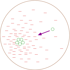
Figure 3: A stack of $\overline{\rm D3}$-branes polarizes the sea of flux, represented by dashes, leading to a force on a test $\overline{\rm D3}$-brane.

One may intuitively understand these results as follows. We can think of the flux background effectively as a sea of D3-branes; it carries D3 charge, as well as some energy-momentum. When a stack of $\overline{\rm D3}$-branes is placed in this sea, the background adjusts itself in an attempt to screen the branes, by moving some of the flux closer to the stack. The effective charge of the $\overline{\rm D3}$s is hence reduced, but the stress-energy in their vicinity only becomes greater. Consequently a test $\overline{\rm D3}$-brane will feel a stronger gravitational attraction than Ramond-Ramond repulsion, and will be drawn towards the anti-branes. (See figure 3.) Because of the universal gravitational attraction, the stack is never truly screened, and the effective force only grows larger as more flux is displaced. Moving further away from the stack a greater volume of polarized flux is enclosed, explaining the growth of the effective D3-brane charge with distance (33).

Condition for Slow Roll Inflation

We have developed a physical picture: a test $\overline{\rm D3}$-brane feels an attractive force from another $\overline{\rm D3}$-brane due to the polarization of the background flux. The force falls off with distance like $1/y^{3}$. We will now formulate the condition for slow roll during the resulting motion of the branes, which could last until the exit via nonabelianization is triggered, making this potentially a kind of hybrid inflation stage [29].

Recall that the slow roll parameter $\eta$, which typically imposes the most strict constraints on the potential, is defined as

$$\eta\,\equiv\,{\mbox{\small$M$}}_{\!p}^{2}\;{V^{\prime\prime}\over V}\,.$$ (34)

where $V^{\prime\prime}$ denotes the second derivative of the inflaton potential, defined such that the inflaton kinetic term is canonically normalized. We would like to apply this prescription to our situation.

Starting from our initial condition with $p$ anti-branes scattered randomly over the $S^{3}$, the process of forming a cluster goes in successive steps. First the branes that are nearest to each other form small clumps, which continue to merge with other small clumps until the maximum size cluster is reached. An important difference with the case of brane/anti-brane inflation is that each small cluster retains its non-zero vacuum energy, and only supercritical size clusters can decay and dump their vacuum energy via brane/flux annihilation. How should we choose to parameterize the inflaton field and compute the corresponding slow roll parameters during the accumulation process?

A natural choice for the inflaton field $X$ is to take the square root of the average (distance)² between the branes,

$$X^{2}={1\over p^{2}}\sum_{i\neq j}(y_{i}-y_{j})^{2}.$$ (35)

In the case that the branes are uniformly distributed over the $S^{3}$, one has $X^{2}=2R^{2}$, where $R^{2}=g_{s}M$ is the radius of the $S^{3}$. Given the interbrane potential, which we denote ${\cal V}(y_{i}-y_{j})$, it is possible to compute the average static force on $X$. This computation is outlined in Appendix B, with the following result

$$a_{0}^{2}\ddot{X}\,\simeq\,-p\,{\cal V}^{\prime}(X)\Bigl{(}1-{X^{2}\over 2R^{2}}\Bigr{)}\,\equiv\,a_{0}^{2}V_{\rm eff}^{\prime}(X),\quad\quad R^{2}=g_{s}M$$ (36)

where the interbrane potential ${\cal V}(X)$ reads

$${\cal V}(X)\,=\,{2\pi g_{s}\over g_{s}M}{a_{0}^{4}\over X^{2}}\,.$$ (37)

This result has the expected feature that for a uniform brane distribution, so that $X^{2}=2R^{2}$, the force vanishes. We now compute $V^{\prime\prime}(X)$ by differentiating $V_{\rm eff}^{\prime}(X)$ at $X^{2}=2R^{2}$. We obtain

$$V^{\prime\prime}(X)\simeq{2\pi pg_{s}a_{0}^{2}\over(g_{s}M)^{3}}\,.$$ (38)

The total potential $V$ is twice the energy stored in the anti-brane tension, $V=2pT_{3}a_{0}^{4}/g_{s}$. Putting things together we find

$$|\eta|\,\simeq\;{16\pi^{4}\over g_{s}M^{3}}\;{{\mbox{\small$M$}}_{\!p}^{2}\over a_{0}^{2}{\mbox{\small$M$}}_{\!s}^{2}}\,,$$ (39)

where we have restored $M_{s}$, previously set equal to 1; $a_{0}M_{s}$ is the string scale at the bottom of the throat. So we would get the required amount of inflation in case we could embed our scenario in a rather mildly warped setting, such that

$${a_{0}^{2}{\mbox{\small$M$}}_{\!s}^{2}\over{\mbox{\small$M$}}_{\!p}^{2}}\,\gtrsim{10^{5}\over g_{s}M^{3}}\,.$$ (40)

As mentioned earlier, $M$ can be chosen as large as $10^{3}$ (or even larger). Taking $g_{s}\sim 10^{-1}$, we find that $a_{0}{\mbox{\small$M$}}_{\!s}$ can be a factor of $30$ below the Planck scale. As we will discuss in more detail in §6, this is difficult to realize within the regime of validity of our approximations.

4. Gravity Dual of the Non-Abelian Inflaton

The preceding analysis is only valid so long as the backreaction is small, which is the case outside the anti-brane throat, $y^{4}\gg 4\pi g_{s}p$. As one goes down the throat, $\Phi_{-}$, which was growing as we approached the throat, “turns around” and begins decreasing as (see (26))

$$\Phi_{-}\simeq{2a_{0}^{4}y^{4}\over 4\pi g_{s}p}\,,$$ (41)

which is the usual result for the near-horizon geometry of the stack of branes. The three-form flux (29), however, is forced into blowing up as $G_{+}\sim 1/y^{4}$ to compensate for $\Phi_{-}$ in the $G$ equations of motion (23). We see that once we are within the throat, the fluxes are no longer small and our approximations of the last section break down. What can we learn about the geometry near the anti-branes?

The perturbation of the near-horizon throat of a stack of D3-branes by 3-form flux has been studied in the classic paper of Polchinski and Strassler (PS) [11]. PS found (see sec. III.D) four linearized solutions for $G_{3}$, falling off as powers $y^{p}$ with $p=0,-4,-6,-10$. The $p=0,-10$ solutions are associated with a constant IASD tensor, which is not our situation. The $p=-4,-6$ solutions, on the other hand, are constructed from a constant ISD tensor $T_{3}$ in the anti-brane throat. The solutions are, for $p=-4$,

$$G_{+}={-i2\sqrt{2}\over g_{s}}{R^{4}\over y^{4}}T_{3}\,,\quad\quad G_{-}={-i4\sqrt{2}\over g_{s}}{R^{4}\over y^{4}}(T_{3}-2V_{3})\,,$$ (42)

and for $p=-6$,

$$G_{+}=0\,,\quad\quad G_{-}=\varsigma{R^{6}\over y^{6}}(T_{3}-2V_{3})\,,$$ (43)

where $V_{mnp}\equiv{y^{q}\over y^{2}}(y^{m}T_{qnp}+y^{n}T_{mqp}+y^{p}T_{mnq})$; one may check that $T_{3}-2V_{3}$ is indeed IASD.

We see that our leading $G$ perturbation (29), which we found by matching to the region outside the throat, is of the $p=-4$ form (42), with ISD tensor

$$T_{ijk}\simeq{\epsilon_{ijk}\over\sqrt{2g_{s}M}}\,.$$ (44)

This $p=-4$ solution corresponds in the holographic dual to the addition of a quadratic term in the superpotential of the non-Abelian worldvolume gauge theory, which generates a cubic term in the full potential, of the same form as the matrix potential given in eqn (16). In addition, it generates masses for the fermions and bosons, proportional to $1/\sqrt{2g_{s}M}$. The worldvolume gauge theory description has limited validity, however, since it is strongly coupled. Instead, the system must be studied using the dual supergravity.

Polchinski and Strassler solved for the effect of the flux perturbation on the supergravity geometry and on the location of the $p$ branes generating the throat. Their essential result is that the branes tend to become non-Abelian and balloon up into an 5-brane wrapping a transverse $S^{2}$. The radial motion of the 5-brane is governed by a effective potential drawing it to a certain minimal energy location within the throat geometry. It was further shown that, due to some miraculous cancellations, the exact form of the effective potential is reproduced by a simple probe calculation based on a single 5-brane moving in the original throat geometry.

The result that the branes tend to non-abelianize is, of course, consistent with our own physical picture. The additional lesson that we have now learned, however, is that the potential obtained in [11] is the proper refinement of the 5-brane potential $V_{\rm ef\!f}(\psi)$ given in (19) in the region near $\psi=0$, where the backreaction needs to be taken into account.

This 5-brane potential can be found in section IV.C of [11], eqn. (72). We match their $z$ as $|z|^{2}=y^{2}/2$, and for the NS5-brane, $z$ is real. The potential then becomes

$$V(y)=\alpha y^{2}(y-\beta)^{2}\,,\quad\quad\alpha={a_{0}^{4}\over 16\pi^{5}g_{s}^{3}p}\,,\quad\quad\beta={\pi g_{s}p\over\sqrt{2g_{s}M}}\,.$$ (45)

The quadratic term in (45) is fixed in [11] by supersymmetry. In our situation, supersymmetry is broken by the conflict between the anti-brane throat and the surrounding ISD background. One may wonder, therefore, whether the quadratic term will be absent or modified in our case. This term has a direct dynamical origin, however, in the backreaction of the fluxes on $\Phi_{+}$. We should expect to obtain the same result (45) in any regime where our flux and geometry agree with that of [11].

The potential (45) has two minima, at $y=0$ and $y=\beta$. The former is outside the validity of the supergravity approximation, while the latter is the location where the giant comes to sit. The radius for the giant is

$$y_{0}^{2}={\pi^{2}g_{s}p^{2}\over 2M}\,,$$ (46)

This answer should be compared with the estimate in [10], eqn. (32): $y^{2}=4\pi^{2}g_{s}(p^{2}~{}-~{}1)/M$, which was obtained from the non-Abelian theory, neglecting the gravitational backreaction. One sees that the parametric dependence matches nicely; the difference in the constants can be interpreted as the tendency of the 5-brane to be held back by its own backreaction. Both results, however, apply only in the limit where $p\ll M$. It is easy to verify from the shape of the potential (19), that in case $p/M$ gets close to the critical value $p_{crit}/M\sim.08$, the size of the giant graviton in fact starts to exceed its gravitational radius. Since this is the regime we are interested in, we must conclude that for the near-critical value of $p/M$, the PS potential (45) can be trusted only for $y$ sufficiently smaller than $y_{0}$ given in (46).

Meanwhile, (45) also exhibits a maximum at $y=\beta/2$. It can be shown that this maximum occurs within the regime of validity of the supergravity approximation, and is also just far enough down the throat, so that the PS potential provides a good description. We would like to investigate whether this top of the potential is a viable starting point for a slow-roll evolution of the giant inflaton 5-brane. Can we get a small value for the inflationary parameter $\eta$ there?

Our coordinate $y$ is not canonically normalized: the $y$ kinetic term is proportional to

$$S_{kin}=-{T_{3}p\,a_{0}^{2}\over g_{s}}\int\!d^{4}x\,{1\over 2}(\partial_{\mu}y)^{2}\,.$$ (47)

At the maximum $y=\beta/2$, we find using (45)

$${\partial^{2}V\over\partial y^{2}}\,\simeq\,{p\,a_{0}^{4}\over 32\pi^{3}Mg^{2}_{s}}\qquad\rightarrow\qquad V^{\prime\prime}\,\simeq\;{a_{0}^{2}\over 4g_{s}M}\,.$$ (48)

To estimate the value of the potential $V$ at this maximum, note the contribution $V(\beta/2)$ from the PS potential is much smaller than the overall contribution from the anti-brane tension, $V=2pT_{3}a_{0}^{4}/g_{s}$. Using these facts, a straightforward calculation gives

$$|\eta|\,\simeq\,\,{\pi^{3}\over pM}\;{{\mbox{\small$M$}}_{\!p}^{2}\over a_{0}^{2}{\mbox{\small$M$}}_{\!s}^{2}}$$ (49)

Inflation works provided $|\eta|\,\lesssim\,1/30$, which requires that the ratio of the red-shifted string scale $a_{0}{\mbox{\small$M$}}_{\!s}$ at the bottom of the conifold and the 4-d Planck scale must satisfy the inequality

$${a^{2}_{0}{\mbox{\small$M$}}_{\!s}^{2}\over{\mbox{\small$M$}}_{\!p}^{2}}\;\gtrsim\;{10^{3}\over p\,M}\,.$$ (50)

A possible value of $p\,M$ is of order $10^{5}$. In this case, this inequality implies that $a_{0}{\mbox{\small$M$}}_{\!s}$ is just one order of magnitude below the 4-d Planck scale.

5. Numerical Study of the Rolling Giant Inflaton

Up to now our focus has been on the dynamics at the onset of NS5 brane formation. We now wish to consider the possibility of inflation produced during the rolling phase of the giant inflaton. Examining the potential (19) indeed reveals another promising regime (well studied with the NS5 action). For very small $p/M$, there is a metastable giant graviton vacuum at finite $\psi$. As one increases $p$, there is a critical value $p_{crit}$ above which the metastable vacuum disappears – the anti-D3 branes perturbatively roll to $M-p$ D3 branes, a feature which provides the graceful exit of our inflationary model. As a consequence of this structure, for $p\sim p_{crit}$ there is actually a plateau in the potential (19) at intermediate values of $\psi$. This plateau can be used to provide several e-foldings of inflation at intermediate $\psi$. Hence, the system of $p$ anti-D3s in the warped flux background is rich enough to potentially exhibit several inflationary phases.

Because the dynamics are more involved in the plateau region, we will study them by explicitly setting up the coupled system of scalar and Friedmann equations, and solving these numerically using Mathematica. We find that for fixed $p/M$, the physics is controlled by only one nontrivial parameter (which we call $B$). For clarity, we now derive the explicit form of the equations of motion that we used for numerical integration.

The 5-brane world-volume action reads [10]

$$S_{NS5}=-A_{0}\int d^{4}x\sqrt{-g_{4}}\left[V_{2}(\psi)\sqrt{1-Z^{2}\dot{\psi}^{2}}+{1\over\pi}U(\psi)\right]\,,$$ (51)

with $V_{2}(\psi)$ and $U(\psi)$ as in (20), and

$$A_{0}\equiv{\mu_{3}Ma_{0}^{4}\over g_{s}}\,,\quad\quad Z^{2}\equiv{g_{s}M\over a_{0}^{2}}\,.$$ (52)

The 5-brane equations of motion are most conveniently expressed in first-order Hamiltonian form. The conjugate momentum derived from (51) is

$$P=A_{0}V_{2}(\psi){Z^{2}\dot{\psi}\over\sqrt{1-Z^{2}\dot{\psi}^{2}}}\,,$$ (53)

leading to the Hamiltonian

$${\cal H}=\sqrt{P^{2}/Z^{2}+A_{0}^{2}\,V_{2}(\psi)^{2}}+{A_{0}\over\pi}U(\psi)\,.$$ (54)

Hamilton’s equations are

$$\dot{\psi}={\partial{\cal H}\over\partial P} = {P\over Z^{2}\sqrt{P^{2}/Z^{2}+A_{0}^{2}\,V_{2}(\psi)^{2}}}\,,$$ (55)

$$\dot{P}=-{\partial{\cal H}\over\partial\psi} = {A_{0}\over\pi}(\cos 2\psi-1)-{A_{0}^{2}\,(4\sin^{3}\psi\cos\psi+2U(\psi)(\cos 2\psi-1))\over 2\pi^{2}\sqrt{P^{2}/Z^{2}+A_{0}^{2}\,V_{2}(\psi)^{2}}}\,.$$

We couple to 4-d gravity:

$$S_{tot}={\mbox{\small$M$}}_{\!p}^{2}\int d^{4}x\sqrt{-g_{4}}{\cal R}+S_{NS5}\,,$$ (56)

and assume a flat FRW universe,

$$g_{\mu\nu}dx^{\mu}dx^{\nu}=-dt^{2}+a(t)^{2}d\vec{x}^{2}\,.$$ (57)

Since we are assuming only time derivatives in $S_{NS5}$, the scale factor is present only in the overall $\sqrt{-g_{4}}$. Hence it can be taken into account by scaling $A_{0}\rightarrow a^{3}A_{0}$ in (55), (S5.Ex1). The Friedmann equation is (written in terms of the momentum $P$)

$$\left({\dot{a}\over a}\right)^{2}={\mu_{3}Ma_{0}^{4}\over 6\pi g_{s}{\mbox{\small$M$}}_{\!p}^{2}}\left[\sqrt{P^{2}\pi^{2}/(A_{0}^{3}a^{6})+\sin^{4}\psi+U(\psi)^{2}}+U(\psi)\right]\,.$$ (58)

We find it convenient to define the variables $\tilde{a}^{3}\equiv A_{0}a^{3}/\pi$, $\tilde{P}\equiv P/Z$, in which case we can write the three coupled first-order equations as

$$Z\dot{\psi} = {\tilde{P}\over\sqrt{\tilde{P}^{2}+\tilde{a}^{6}\,\pi^{2}V_{2}(\psi)^{2}}}\,,$$

$$Z\dot{\tilde{P}} = \tilde{a}^{3}(\cos 2\psi-1)-{\tilde{a}^{6}\,(4\sin^{3}\psi\cos\psi+2U(\psi)(\cos 2\psi-1))\over 2\sqrt{\tilde{P}^{2}+\tilde{a}^{6}\,\pi^{2}V_{2}(\psi)^{2}}}\,,$$ (59)

$$Z\dot{\tilde{a}} = \tilde{a}\sqrt{B}\left[\sqrt{\tilde{P}^{2}\tilde{a}^{-6}+\sin^{4}\psi+U(\psi)^{2}}+U(\psi)\right]^{1/2}\,,$$

with

$$B\equiv{Z^{2}\mu_{3}Ma_{0}^{4}\over 6\pi g_{s}{\mbox{\small$M$}}_{\!p}^{2}}={M^{2}\over 48\pi^{4}}\;{a_{0}^{2}{\mbox{\small$M$}}_{\!s}^{2}\over{\mbox{\small$M$}}_{\!p}^{2}}\,.$$ (60)

We solved these equations numerically. Notice that $Z$ now appears in combination with the time derivative, and thus can be absorbed into a new definition of time. Hence the relevant parameters for controlling the dynamics are just $B$ and $Y\equiv\pi p/M$; for $p=p_{crit}$ we have $Y\sim 2/7$.

Figure 4: The giant inflaton trajectory for $B=0.85$ and initial conditions $\psi(0)=.03$ and $\tilde{P}(0)=0.3$, and the corresponding evolution in the log of the scale factor $a$. We see that almost all of the inflation comes from the shoulder region near $\psi=0.7$.

In figure 4, we have indicated a typical trajectory for $B\sim.85$, and $Y=2/7$. The initial conditions chosen are $\psi(0)=1/25$ and $\tilde{P}(0)=0.3$. The evolution is insensitive to the initial condition of $\psi$ as long as it is near zero. We see that one quite easily obtains $\sim 60$ e-foldings of exponential expansion, with quite generic initial conditions. All of the expansion is generated in the shoulder region, where the potential flattens out. If one allows for smaller initial momenta, we find that one can still get around 60 e-foldings for values of $B\simeq 0.5$.

Hence given the expression (60) for $B$, we conclude that the rolling giant inflaton can represent an interesting scenario provided that it can be realized with a mild enough warp factor $a_{0}$. The condition on $a_{0}$ is roughly

$${a_{0}{\mbox{\small$M$}}_{\!s}\over{\mbox{\small$M$}}_{\!p}}\gtrsim{65\over M}\,.$$ (61)

Note that this condition is slightly less stringent than (50), given that $p/M\sim 10^{-1}$. In the next section we will analyze whether this condition can be satisfied within our set-up.

6. The Viability of the Giant Inflaton

In the previous sections, we have expressed the conditions for inflation in terms of specific inequalities (40), (50) and (61) for the ratio of the red-shifted string scale $a_{0}{\mbox{\small$M$}}_{\!s}$ and the 4-d Planck scale ${\mbox{\small$M$}}_{\!p}$. The inequalities also involve the microscopic parameters $M$, $p$ and $g_{s}$; the ratio $a_{0}{\mbox{\small$M$}}_{\!s}/{\mbox{\small$M$}}_{\!p}$ is not independent of these quantities. In this final section we will study whether the inequality can be satisfied within our set-up.

The 4-d Planck scale is expressed in string units as

$${\mbox{\small$M$}}_{\!p}^{2}={V_{6}\over g_{s}^{2}\kappa_{10}^{2}}\,,\quad\quad\kappa_{10}^{2}=\pi(2\pi)^{6}\,,$$ (62)

where $V_{6}$ is the warped volume of the compactification manifold. We wish to obtain an estimate of the minimal possible value of $V_{6}$ for given flux $M$ and $K$. To this end, let us compute the warped volume of the throat region. In the warped region between the tip and the Calabi-Yau manifold, the throat geometry takes the approximate form

$$\tilde{g}_{mn}dy^{m}dy^{n}=dy^{2}+y^{2}ds_{T^{1,1}}^{2}\,,\quad e^{-4A}\approx{R^{4}\over y^{4}}\,,\quad R^{4}\approx{27\pi\over 4}\,g_{s}MK\,,$$ (63)

giving a total space that is approximately $AdS_{5}\times T^{1,1}$, where $T^{1,1}$ is the base of the conifold. We can now perform the integral

$$V_{6}\equiv\int\!\!d^{6}y\,\sqrt{\tilde{g}_{6}}\,e^{-4A}\! \!\simeq\! \!\int_{T^{1,1}}\!\!\!d\Omega\;\int_{y_{0}}^{y_{1}}\!\!\!\!dy\,y^{5}\,{R^{4}\over y^{4}}\ \simeq\ {1\over 2}\,{\rm vol}(T^{1,1})\,R^{6}\,,$$ (64)

where in the last line we assume that the location $y_{0}$ of the bottom of the throat is small compared to the location $y_{1}\sim R$ where the throat is capped off by the CY geometry. Plugging in the values for $R^{6}$ and the known volume of $T^{1,1}$, we thus obtain a lower bound for the total warped 6-volume, given by

$$V_{6}\gtrsim\Bigl{(}{2\pi\over 3}\Bigr{)}^{3}\Bigl{(}{27\pi\over 4}\,g_{s}MK\Bigr{)}^{3/2}$$ (65)

The warp factor at the bottom of the KS throat scales with powers of the overall volume, as well as the complex structure $z$ of the conifold geometry, which is also determined by the microscopic parameters:

$$a_{0}^{2}\simeq{V_{6}^{1/3}z^{2/3}\over g_{s}M}\;\,,\quad\quad z\simeq e^{-{2\pi K\over g_{s}M}}\,.$$ (66)

Combined we derive the following inequality for the ratio of the warped string scale and the 4-d Planck scale:

$${a_{0}^{2}{\mbox{\small$M$}}_{\!s}^{2}\over{\mbox{\small$M$}}_{\!p}^{2}}\,=\,{g_{s}^{2}\,a_{0}^{2}\,\kappa_{10}^{2}\over V_{6}}\;\lesssim\;{64\pi^{4}z^{2/3}\over 3M^{2}K}\,.$$ (67)

This inequality should be compared with our conditions (40), (50) (61) for inflation.

The most promising stage for inflation, it turns out, is stage I, the accumulation process of the anti-branes on the $S^{3}$. Combining the result (39) of §3 and the estimate (67) we obtain the lower bound for $|\eta|$ during this stage

$$|\eta|\gtrsim{{3K\over 4g_{s}M}\,\exp\Bigl{(}{4\pi K\over 3g_{s}M}\Bigr{)}}\,.$$ (68)

Given this formula, slow roll would require that $g_{s}M$ is at least 30 times larger than $K$, which would correspond to a very shallow, mildly warped throat.

Such a shallow throat is problematic for our approximations, however. Our description in terms of the conifold geometry holds only for $z\ll 1$, which requires $K$ to be larger than $g_{s}M$. This renders our conclusion that inflation works in the regime (68) suspect. For this reason, we will not try to analyze the inflationary predictions in any detail. It would be interesting (though technically challenging) to study this scenario in a global setting where the calculations could be continued beyond our present regime of control.

The analogous results for the giant inflaton moving in its own throat (39), and rolling over the shoulder (60) are

$$|\eta|\simeq{3MK\over 64\pi p}\exp\Bigl{(}{4\pi K\over 3g_{s}M}\Bigr{)}\,,$$ (69)

and

$$B^{-1}={9K\over 4}\exp\Bigl{(}{4\pi K\over 3g_{s}M}\Bigr{)}\,.$$ (70)

The throat roll result (69) is moderately larger than (68), by a factor $(g_{s}M)(M/p)/(16\pi)$. $B^{-1}$ is larger than (68) by $3g_{s}M$, but as we discussed $B^{-1}$ can be as large as $1$ or $2$. All three results are tantalizingly close to realizability, but lie just outside the bounds of our approximations. It is intriguing to speculate that if we could gain control of the region $K\ll g_{s}M$, these giant inflaton scenarios could be realized.

7. Discussion

Our results illustrate several simple points about brane cosmology in string theory. Among them:

$\bullet$ Unlike the models described in [9], in the promising regime of parameters these models provide inflation at a very high scale. This exacerbates the challenges of moduli stabilization (one must make sure the the radion and dilaton are stiff already at this very high $V^{1/4}$), but relaxes the tuning associated with obtaining initial conditions appropriate for low-scale inflation. Indeed, even if the 60+ e-foldings which explain our flat, homogeneous bubble occur at $V^{1/4}<<{\mbox{\small$M$}}_{\!s}$, it is natural to postulate a primordial phase of inflation very close to $V^{1/4}\sim{\mbox{\small$M$}}_{\!s}$ to explain the initial conditions for the later stage. The giant inflaton could provide a model of this “primordial inflation,” which can occur at a very high scale and need not last for 60 e-foldings.

$\bullet$ Unlike the models described in [9], here we see that warping actually works $\it against$ the success of many potential models. We have always assumed very mild warping $a_{0}$ in the inflationary throat, because our slow-roll parameters scale like $1/a_{0}^{2}$. The reason for the difference between this class of models and the models of [9] arises because only potentials which are inverse power laws in the canonical inflaton field provide improved inflationary properties in warped backgrounds. More conventional field theoretic models with positive power-law potentials (analogous to the effective field theories which arise in our models) are hindered by the warping.

$\bullet$ The emergence of the standard model at the end of inflation may be more “stringy” than is assumed in the most conventional models. For instance, in brane/anti-brane scenarios, it is natural to assume that the standard model branes (plus an extra) are the targets which collide with an anti-brane to end inflation; then the standard-model open strings are naturally excited in a reheating process during the brane/anti-brane annihilation. In such a model, the standard model degrees of freedom are already evident as perturbative quantum fields during inflation. In a scenario like ours, it is possible for the standard model to emerge on the $M-p$ D3 branes which only exist $\it after$ the brane/flux annihilation is completed. In this sense the standard model degrees of freedom may only emerge as perturbative objects at the end of inflation.

$\bullet$ One merit of exhibiting an inflationary scenario within a microscopically complete theory is that it allows one to examine the nature and severity of the required tunings to produce inflation. As in [9], we find that tuning is required to produce a working model in our scenario. However, the tuning can be explicitly parameterized in terms of microscopic data which is at our disposal – the choice of the number of anti-D3 branes $p$ and the background RR flux $M$. The severity (or lack thereof) of the tuning may be best estimated not by assuming a flat measure on e.g. $\eta$ space, but instead by asking: how severely must we tune the microscopic parameters within their reasonable ranges, to obtain a desirable value of $\eta$? In the case at hand, it looks a bit worse than one would have expected, but there is no reason to expect that this is a general feature.

Acknowledgments

We would like to thank Kristin Burgess, Renata Kallosh, Andrei Linde, John McGreevy, Eva Silverstein and Lenny Susskind for discussions. We are particularly grateful to John Pearson for early collaboration. This material is based upon work supported by the National Science Foundation under grants No. 0243680 (O.D. and H.V.) and PHY-0097915 (S.K.). Any opinions, findings, and conclusions or recommendations expressed in this material are those of the authors and do not necessarily reflect the views of the National Science Foundation. The work of S.K. was also supported by a David and Lucile Packard Foundation Fellowship for Science and Engineering, and the DOE under contract DE-AC03-76SF00515.

Appendix A Forces generated by distant fluxes

In compactifying the KS throat as in [12], one introduces other fluxes elsewhere in the Calabi-Yau manifold. These will generically backreact and produce perturbations to the KS throat. Here we show that these corrections break the Goldstone-mode shift symmetry on the $S^{3}$ for the D-brane collective coordinates. We present two arguments: a direct gravity-side estimate, and a dual holographic field theory estimate. The two agree. The gravity estimate basically uses the same logic as [30], which studied soft-breaking terms in flux compactifications.

A.1 Anti-D3 potential from distant fluxes

We consider “distant fluxes” supported on cycles not associated with our throat, but preserving the ISD property. The effect on the warp factor can be determined from the equation of motion (7) with $\alpha=e^{4A}$ and ${\cal R}_{4}=0$,

$$\nabla^{2}A={g_{s}^{2}|G|^{2}\over 48}\,,$$ (71)

where to this order we are ignoring the tension of the anti-branes. The leading contribution to $|G|^{2}$ comes from the primary fluxes $M$ and $K$, which of course generates the radial warp factor (63) respecting the $SO(4)$-symmetry. We consider the subleading corrections involving the distant fluxes.

The primary flux at the base of the throat is equal to

$$G_{mnp}={2M\epsilon_{mnp}\over(g_{s}M)^{3/2}}\,,$$ (72)

in terms of the warped epsilon tensor of the 3-sphere. A natural estimate for the distant flux is that is proportional, up to some factor $f$ of order unity, to the unwarped volume of the $S^{3}$:

$$\delta G_{mnp}\sim f\Omega_{mnp}\sim{fz\epsilon_{mnp}\over(g_{s}M)^{3/2}}\,,$$ (73)

where we used that $\int_{A}\Omega=z$. One way of thinking about this is that the density of primary flux must be very large in unwarped units, since it is integrated over a small cycle to obtain a fixed value $M$. The distant fluxes will generically be associated to a cycle of order one, and hence the density of the flux will be smaller, by an order $z$.

The subleading value of $|G|^{2}$ is then

$${g_{s}^{2}(G_{mnp}\,\delta\overline{G}^{mnp}+\delta G_{mnp}\overline{G}^{mnp})\over 48}\sim{fz\over 2g_{s}M^{2}}\,\equiv\,{1\over 8}m_{{}_{\!X}}^{2}a_{0}^{-2}\quad\rightarrow\quad m_{X}^{2}={4fza_{0}^{2}\over g_{s}M^{2}}\,.$$ (74)

Considering only the variation of the warp factor over the $S^{3}$, we then estimate

$$A(\Phi)\sim A_{0}+{1\over 8}m_{{}_{\!X}}^{2}a_{0}^{-2}g_{ij}\Phi^{i}\Phi^{j}+\ldots\,,$$ (75)

and find that $m_{X}^{2}$ is the effective mass for canonically normalized fields $X^{i}\equiv a_{0}\sqrt{T_{3}M}\Phi^{i}$,

$$S_{\overline{\rm D3}} \sim -\int d^{4}x\sqrt{-g_{4}}\,\left({2T_{3}pa_{0}^{4}\over g_{s}}+{1\over 2}m_{{}_{\!X}}^{2}\,{\rm Tr}\,X_{i}^{2}+{1\over 2}\,{\rm Tr}\,(\partial_{\mu}X_{i})^{2}\right)\,.$$ (76)

All mass-scales in the above formulas are expressed in units of the unwarped string scale ${\mbox{\small$M$}}_{\!s}$. We see that beyond the overall redshift of $a_{0}$ that affects all masses at the bottom of the throat, the mass-squared $m_{{}_{\!X}}^{2}$ induced by distant fluxes is suppressed by an additional factor of $z=\exp(-2\pi K/3g_{s}M)$.

One may easily impose a discrete symmetry on the geometry such that the crossterm (74) vanishes. In this case, the leading mass correction is instead

$${g_{s}^{2}\delta G_{mnp}\delta\overline{G}^{mnp}\over 48}\sim{f^{2}z^{2}\over 8g_{s}M^{3}}\equiv{1\over 8}m_{X}^{2}a_{0}^{-2}\quad\rightarrow\quad m^{2}_{X}={f^{2}z^{2}a_{0}^{2}\over g_{s}M^{3}}\,.$$ (77)

which is suppressed by two factors of $z$. The masses in (74), (77) are smaller than the effective mass from interbrane forces (38), and hence we neglect them in our estimates of inflation.

A.2 Holographic argument

It is instructive to consider these symmetry breaking perturbations from the point of view of the holographic dual picture. The Klebanov-Strassler geometry has a dual description as a four-dimensional ${\cal N}=1$ $SU(M(K+1))\times SU(MK)$ field theory with bi-fundamental fields $A_{i}$, $B_{j}$ transforming in the $({\bf 2},{\bf 1})$ and $({\bf 1},{\bf 2})$ of $SO(4)\sim SU(2)\times SU(2)$ and a quartic superpotential. The rest of the geometry at the top of the KS throat can be interpreted as a “Planck brane” in the spirit of [31], corresponding to additional dynamics cutting the theory off in the UV, at the Planck scale. This is realized as irrelevant operators suppressed by powers of ${\mbox{\small$M$}}_{\!p}$ added to the dual field theory.

The $SO(4)$-breaking physics of the distant fluxes is hence translated into $SO(4)$-breaking irrelevant operators in the dual. One can estimate these as follows. Assuming unbroken supersymmetry, we consider corrections to the superpotential. The most straightforward class of these is (see [32]):

$$\Delta W_{n}={\cal C}^{i_{1}i_{2}\ldots i_{n}j_{i}j_{2}\ldots j_{n}}\,{\rm Tr}\left(A_{i_{1}}B_{j_{1}}A_{i_{2}}B_{j_{2}}\ldots A_{i_{n}}B_{j_{n}}\right)\,.$$ (78)

For generic choices of ${\cal C}$, $SO(4)$ is broken. Due to the anomalous dimensions of the $A_{i},B_{j}$ fields, these perturbations have dimension $\Delta_{n}=3n/2$. The superpotential of the theory, which is marginal, is a special case of $n=2$. Hence the leading irrelevant operator has $n=3$ and dimension $\Delta=9/2$, while the subleading irrelevant perturbation is $n=4$ with $\Delta=6$. The corresponding terms in the component Lagrangian have dimension $(3/2)(2n-1)-1/2=3n-2$, and hence we find perturbing irrelevant operators ${\cal O}_{7}$ and ${\cal O}_{10}$.

We can obtain mass terms for brane modes at the bottom of the throat by substituting some of the $A$s and $B$s in each ${\cal O}$ with their VEV, leaving a mass term (i.e. the operators are “dangerously irrelevant”). At the bottom of the throat these VEVs are naturally of the scale $a_{0}{\mbox{\small$M$}}_{\!p}$. Hence a mass term from of ${\cal O}_{7}$, will naturally scale like $m^{2}\sim(a_{0})^{5}$, while a mass term from ${\cal O}_{10}$ behaves as $m^{2}\sim(a_{0})^{8}$. Recalling that $z\sim a_{0}^{3}$, These are precisely the results for the leading (74) and subleading (77) perturbations from distant flux we found above, confirming from the dual field theory point of view that these are the appropriate corrections to the KS throat.

This analysis naturally suggests that it is possible to forbid the larger mass term (74), leaving the smaller (77) as the leading correction, by imposing a discrete symmetry. For example, $A_{i}\rightarrow-A_{i}$, $B_{j}\rightarrow B_{j}$ is a symmetry of the KS field theory dual. It can be mapped into a symmetry of the geometry as in [32]. Requiring that such a $Z_{2}$ symmetry can be extended to hold throughout the geometry is enough to forbid (74). It is easy to find examples of Calabi-Yau manifolds which admit such a global $Z_{2}$ symmetry.

Appendix B Computation of Effective Potential $V_{\rm eff}(X)$

In this appendix we outline the derivation of eqn (36). Consider $p$ particles on a sphere with radius $R$. We assume that $p$ is large, and will work to leading order in $p$. Particle $i$ has a position ${\vec{x}}_{i}$ satisfying $|\vec{x}_{i}|^{2}=R^{2}$. The particles interact via a potential

$$V(x_{ij})=(x_{ij})^{n}\,\qquad\quad x_{ij}=|{\vec{x}}_{i}-{\vec{x}}_{j}|.$$ (79)

Define $X$ as the square root of the average (distance)² between the particles

$$X^{2}={1\over p^{2}}\sum_{i\neq j}(x_{ij})^{2}$$ (80)

Let us assume that the motion of the particles is governed by the Lagrangian

$$L={1\over 2}\sum_{i}\dot{x}^{2}_{i}-\sum_{i<j}V(x_{ij})-\sum_{i}\lambda_{i}(x_{i}^{2}-R^{2}),$$ (81)

with corresponding equation of motion

$$\ddot{\vec{x}}_{i}=-\sum_{k\neq i}\hat{x}_{ik}V^{\prime}(x_{ik})-2\lambda_{i}{\vec{x}}_{i}$$ (82)

Starting with all particles at rest, we want to compute the second time derivative $\ddot{X}$. We start from

$$X\ddot{X} \!=\! {1\over p^{2}}\sum_{i\neq j}{\vec{x}}_{ij}\!\cdot(\ddot{\vec{x}}_{i}-\ddot{\vec{x}}_{j})$$ (83)

The plan is to evaluate the right-hand side by inserting the equation of motion (82). This still results in a complicated expression. However, we can simplify the calculation by treating the Lagrange multipliers $\lambda_{i}$ in a “mean field” approximation, setting

$$\lambda_{i}=\lambda_{j}=\lambda$$ (84)

The mean field value is determined by the condition that

$$\sum_{i}{\vec{x}}_{i}\!\cdot\ddot{\vec{x}}_{i} \!=\! -\sum_{i\neq j}{\vec{x}}_{i}\!\cdot\hat{x}_{ij}V^{\prime}(x_{ij})-2\lambda\sum_{i}x_{i}^{2}$$ (85)

$$\!=\! -{1\over 2}\sum_{i\neq j}{x}_{ij}\,V^{\prime}(x_{ij})\;-\;2\lambda\,p\,R^{2}\,=\,0$$

We thus find

$$\lambda={npV\over 4\,R^{2}}\,\qquad\quad V\equiv{1\over p^{2}}\sum_{i\neq j}V(x_{ij})$$ (86)

A straightforward calculation now gives

$$X\ddot{X} \!=\! {1\over p}\sum_{i\neq j}{x}_{ij}\,V^{\prime}(x_{ij})\,-\,{2\lambda\over p^{2}}\sum_{i\neq j}x_{ij}^{2}$$ (87)

$$\!=\! \Bigl{(}1-{X^{2}\over 2R^{2}}\Bigr{)}\,p\,nV$$

Identifying $nV=XV^{\prime}(X)$ gives equation (36).

References

-
[1]
A. Guth, “The Inflationary Universe: A Possible Solution to the
Horizon and Flatness Problems,” Phys. Rev. D23, 347
(1981);
A. Linde, “A New Inflationary Universe Scenario: A Possible Solution of the Horizon, Flatness, Homogeneity, Isotropy and Primordial Monopole Problems,” Phys. Lett. B108 (1982) 389;
A. Albrecht and P. Steinhardt, “Cosmology for Grand Unified Theories with Radiatively Induced Symmetry Breaking,” Phys. Rev. Lett. 48 (1982) 1220. - [2] S. Kachru, R. Kallosh, A. Linde and S. P. Trivedi, “De Sitter vacua in string theory,” Phys. Rev. D 68, 046005 (2003) [arXiv:hep-th/0301240].
- [3] C.P. Burgess, R. Kallosh and F. Quevedo, “De Sitter String Vacua from Supersymmetric D-terms,” JHEP 0310 (2003) 056, hep-th/0309187.
- [4] A. Saltman and E. Silverstein, “The Scaling of the No-Scale Potential and de Sitter Model Building,” hep-th/0402135.
- [5] A. Frey, M. Lippert and B. Williams, “The Fall of Stringy de Sitter,” Phys. Rev. D68 (2003) 046008, hep-th/0305018.
- [6] C. Escoda, M. Gomez-Reino and F. Quevedo, “Saltatory de Sitter String Vacua,” JHEP 0311 (2003) 065, hep-th/0307160.
- [7] R. Brustein and S. P. de Alwis, “Moduli potentials in string compactifications with fluxes: Mapping the discretuum,” arXiv:hep-th/0402088.
-
[8]
G.R. Dvali and S.H. Tye, “Brane Inflation,” Phys. Lett. B450 (1999) 72, hep-th/9812483;
S.H. Alexander, “Inflation from D -anti D brane annihilation,” Phys. Rev. D65 (2002) 023507, hep-th/0105032;
C.P. Burgess, M. Majumdar, D. Nolte, F. Quevedo, G. Rajesh and R.J. Zhang, “The inflationary brane-antibrane universe,” JHEP 0107 (2001) 047,hep-th/0105204;
G.R. Dvali, Q. Shafi and S. Solganik, “D-brane Inflation,” hep-th/0105203. - [9] S. Kachru, R. Kallosh, A. Linde, J. Maldacena, L. McAllister and S. P. Trivedi, “Towards inflation in string theory,” JCAP 0310, 013 (2003) [arXiv:hep-th/0308055].
- [10] S. Kachru, J. Pearson and H. Verlinde, “Brane/flux annihilation and the string dual of a non-supersymmetric field theory,” JHEP 0206, 021 (2002) [arXiv:hep-th/0112197].
- [11] J. Polchinski and M. J. Strassler, “The string dual of a confining four-dimensional gauge theory,” arXiv:hep-th/0003136.
- [12] S. B. Giddings, S. Kachru and J. Polchinski, “Hierarchies from fluxes in string compactifications,” Phys. Rev. D 66, 106006 (2002) [arXiv:hep-th/0105097].
- [13] I. R. Klebanov and M. J. Strassler, “Supergravity and a confining gauge theory: Duality cascades and SB-resolution of naked singularities,” JHEP 0008, 052 (2000) [arXiv:hep-th/0007191].
- [14] R. Myers, “Dielectric Branes,” JHEP 9912, 022 (1999) [hep-th/9910053].
- [15] L. Pilo, A. Riotto and A. Zaffaroni, “Old inflation in string theory,” hep-th/0401004.
-
[16]
J. Hsu, R. Kallosh and S. Prokushkin, “On Brane Inflation with
Volume Stabilization,” hep-th/0311077;
H. Firouzjahi and S.H. Tye, “Closer Towards Inflation in String Theory,” hep-th/0312020. - [17] E. Silverstein and D. Tong, “Scalar Speed Limits and Cosmology: Acceleration from D-cceleration,” hep-th/0310221.
- [18] A. Buchel and R. Roiban, “Inflation in warped geometries,” arXiv:hep-th/0311154.
- [19] M. R. Garousi, M. Sami and S. Tsujikawa, “Inflation and dark energy arising from rolling massive scalar field on the D-brane,” arXiv:hep-th/0402075.
- [20] A. Buchel, “Gauge theories on hyperbolic spaces and dual wormhole instabilities,” arXiv:hep-th/0402174.
- [21] C.P. Burgess, J.M. Cline, H. Stoica and F. Quevedo, “Inflation in Realistic D-brane Models,” hep-th/0403119.
-
[22]
K. Becker and M. Becker, “M-theory on Eight Manifolds,” Nucl.
Phys. B477 (1996) 155;
S. Sethi, C. Vafa and E. Witten, “Constraints on Low Dimensional String Compactifications,” Nucl. Phys. B480 (1996) 213, hep-th/9606122. -
[23]
S. Gukov, C. Vafa and E. Witten, “CFTs from
Calabi-Yau Fourfolds,” Nucl. Phys. B584, 69 (2000) [hep-th/9906070];
T.R. Taylor and C. Vafa, “RR Flux on Calabi-Yau and Partial Supersymmetry Breaking,” Phys. Lett. B474 (2000) 130, hep-th/9912152;
P. Mayr, “On Supersymmetry Breaking in String Theory and its Realization in Brane Worlds,” Nucl. Phys. B593 (2001) 99, hep-th/0003198. -
[24]
K. Dasgupta, G. Rajesh, and S. Sethi, “M-theory, Orientifolds and
G-flux,” JHEP 9908, 023 (1999) [hep-th/9908088];
B. Greene, K. Schalm and G. Shiu, “Warped Compactifications in M and F-theory,” Nucl. Phys. B584, 480 (2000) [hep-th/0004103]. - [25] O. DeWolfe and S. B. Giddings, “Scales and hierarchies in warped compactifications and brane worlds,” Phys. Rev. D 67, 066008 (2003) [arXiv:hep-th/0208123].
- [26] C. Herzog, I. Klebanov and P. Ouyang, “Remarks on the Warped Deformed Conifold,” [hep-th/0108101].
- [27] D. Jatkar, G. Mandal, S. Wadia and K. Yogendran, “Matrix dynamics of fuzzy spheres,” hep-th/0110172.
-
[28]
H. Verlinde, “Holography and Compactification,”
Nucl. Phys. B580, 264 (2000) [hep-th/9906182];
C. Chan, P. Paul and H. Verlinde, “A Note on Warped String Compactification,” Nucl. Phys. B581, 156 (2000) [hep-th/0003236]. - [29] A.D. Linde, “Hybrid Inflation,” Phys. Rev. D49 (1994) 748, astro-ph/9307002.
-
[30]
P.G. Camara, L.E. Ibanez and A.M. Uranga, “Flux Induced SUSY
Breaking Soft Terms,” hep-th/0311241;
for related work see M. Grana, T. Grimm, H. Jockers and J. Louis, “Soft Supersymmetry Breaking in Calabi-Yau Orientifolds with D-branes and Fluxes,” hep-th/0312232;
A. Lawrence and J. McGreevy, “Local String Models of Soft Supersymmetry Breaking,” hep-th/0401034. - [31] L. Randall and R. Sundrum, “A Large Mass Hierarchy from a Small Extra Dimension,” Phys. Rev. Lett. 83, 3370 (1999) [hep-th/9905221].
- [32] I. R. Klebanov and E. Witten, “Superconformal field theory on three-branes at a Calabi-Yau singularity,” Nucl. Phys. B 536, 199 (1998) [arXiv:hep-th/9807080].