Inflation in Realistic D-Brane Models

Abstract:

We find successful models of D-brane/anti-brane inflation within a string context. We work within the GKP-IKLT class of type IIB string vacua for which many moduli are stabilized through fluxes, as recently modified to include ‘realistic’ orbifold sectors containing standard-model type particles. We allow all moduli to roll when searching for inflationary solutions and find that inflation is not generic inasmuch as special choices must be made for the parameters describing the vacuum. But given these choices inflation can occur for a reasonably wide range of initial conditions for the brane and antibrane. We find that D-terms associated with the orbifold blowing-up modes play an important role in the inflationary dynamics. Since the models contain a standard-model-like sector after inflation, they open up the possibility of addressing reheating issues. We calculate predictions for the CMB temperature fluctuations and find that these can be consistent with observations, but are generically not deep within the scale-invariant regime and so can allow appreciable values for $dn_{s}/d\ln k$ as well as predicting a potentially observable gravity-wave signal. It is also possible to generate some admixture of isocurvature fluctuations.

1 Introduction

The possibility of having cosmological inflation arise due to the relative motion of D-branes and their anti-branes is very attractive [1, 2, 3]. It provides an explicit and geometrical interpretation of the inflaton field as the separation of the D-branes [6], with slow roll potentially achieved through a calculably weak effective attraction. It also includes a naturally graceful exit from inflation due to the necessary appearance of an open string tachyon at a critical separation [1], providing a stringy realization of the hybrid inflation [7] scenario. This potentially permits further connections between cosmology and string theory through the properties of the tachyon field which have been recently discovered [8].

Its great promise as an inflationary mechanism has sharpened the search for an explicit realization of this scenario within a string compactification. This search has proven to be difficult, for several reasons. First, as originally pointed out in [1], slow roll generically does not occur for brane motion in compact spaces because the branes typically cannot get far enough apart to let their interactions become sufficiently weak. Compact spaces also raise another difficulty, since the projecting out of bulk-field zero modes also makes slow rolls difficult to achieve [9]. (See [10] for a recent discussion of ways to avoid this last difficulty.)

A second serious obstacle has been the strong technical assumption (made in all of the original proposals) that all string moduli but the putative inflaton be fixed by some unknown string effect. Recent progress circumventing this difficulty has come with the realization that string moduli can be explicitly fixed if the extra dimensions are appropriately warped due to the presence of fluxes [11]. However even in this case inter-brane inflation has been difficult to obtain [9] due to a variant of the standard $\eta$-problem of supergravity inflationary models [12]. It is nonetheless expected that inflation can occur in these vacua, although possibly at the expense of fine tunings in the brane initial conditions to roughly a part in 100.

Model-building suggests two features to seek in any inflationary candidate within string theory. First, resolution of the $\eta$ problem suggests looking for a $D$-term inflationary mechanism [13, 14], with the inflationary energy density being driven by a supersymmetric $D$-term which is independent of (or weakly dependent on) the putative inflaton. Second, successful post-inflationary reheating requires the model be realistic in the sense that it is possible to identify where Standard Model degrees of freedom reside once inflation ends. The challenge is to find real string vacua with these features, and for which as many moduli are fixed as possible. This is the motivation for the present paper, and we find that the inclusion of Standard Model sectors automatically introduces $D$-term potentials.

We base our inflationary scenario on a recent extension to realistic models [15] of the IKLT mechanism [11] for moduli stabilization. The extension we use requires adding extra branes where the (chiral) standard model particles can sit. These models are particularly attractive for our purposes because they incorporate many desirable features for phenomenology. Besides including the spectrum of the standard model with three chiral families of quarks and leptons, they also include a mechanism for fixing the moduli and for generating a hierarchy through warping, à la Randall and Sundrum [16]-[19]. The models considered necessarily require more than one Kähler modulus to be present and therefore the effective potential depends on more than the few fields of the IKLT scenario. We identify here the essential low-energy features of this scenario in order to explore their prospects for obtaining inflation.

We organize our presentation as follows. In order to set the stage for our own work, in the next section we briefly summarize recent developments, including both the string vacua which arise in the IKLT [11] and IKLIMT [9] cosmological models of recent interest and the construction [15] which allows realistic string vacua to be embedded into these constructions. Section 3 follows this with a description of the effective 4D theory which captures the main features of the low-energy dynamics of the moduli of these string vacua. In section 4 we follow brane-antibrane motion with this low-energy moduli space in search of inflationary slow rolls. In certain circumstances we are able to identify sufficiently slow rolls and this section describes the required circumstances in detail. In Section 5 we close with some concluding remarks, including some words concerning reheating and whether string theory may prefer to produce a comparatively short period of inflation at the epoch of horizon exit for the largest scales currently observed in the fluctuations of the cosmic microwave background.

2 Fluxes, Warping and Moduli Fixing

Let us in this section briefly summarize the results of [11] which are relevant for our discussion.

2.1 GKP Compactifications

The authors of ref. [11] use the GKP [19] vacua of the Type IIB string, which are compactified in the presence of D-branes and orientifold planes in such a way as to preserve $N=1$ supersymmetry in four dimensions (see also [18] for earlier discussions.). These vacua have RR and NS-NS antisymmetric 3-form field strengths, $H_{3}$ and $F_{3}$ respectively, which can have a (quantized) flux on 3-cycles of the compactification manifold,

$$\frac{1}{4\pi^{2}\alpha^{\prime}}\int_{A}F_{3}\ = J\,,$$ (1)

$$\frac{1}{4\pi^{2}\alpha^{\prime}}\int_{B}H_{3}\ = -K\,,$$ (2)

where $K$ and $J$ are arbitrary integers and $A$ and $B$ are the different 3-cycles of the internal Calabi-Yau manifold.

The 10D field equations imply that the inclusion of fluxes of RR and/or NS-NS forms in the compact space warps the 4D metric according to

$$d\hat{s}_{10}^{2}=A\,z(y)\,g_{\mu\nu}(x)\,dx^{\mu}\,dx^{\nu}+L^{2}\,z^{-1}(y)h_{mn}(y)\,dy^{m}\,dy^{n}\,,$$ (3)

with a warp factor, $z$, which can be computed in regions close to a conifold singularity of the Calabi-Yau manifold. (The $L$-dependent factor $A$ is chosen to ensure the low-energy theory is obtained in the 4D Einstein frame.) The result for the warp factor is exponentially suppressed at the throat’s tip, depending on the fluxes as:

$$z_{0}\sim L^{2}\,e^{-2\pi K/3g_{s}J}\,,$$ (4)

where $g_{s}$ is the string coupling constant. If this warp factor suppresses standard-model particle masses relative to the string scale, then such fluxes can naturally generate a large hierarchy [16].

The fluxes turned on in the GKP construction are also useful for fixing string moduli, since they can stabilize all of those moduli that are associated with the complex structure of the underlying Calabi-Yau space. This includes in particular the axion-dilaton chiral scalar field of type IIB theory, $S=e^{\phi}+i{\hat{a}}$. From the point of view of the 4 dimensional field theory the fluxes generate a superpotential in the effective supergravity action of the Gukov-Vafa-Witten form [20]:

$$W\ =\ \int_{M}G_{3}\wedge\Omega\,,$$ (5)

where $G_{3}=F_{3}-iSH_{3}$ with $S$ the dilaton field and $\Omega$ the unique $(3,0)$ form of the corresponding Calabi-Yau space.

This mechanism does not fix any of the moduli associated with the Kähler class. The simplest models therefore only have one modulus, which is the model-independent Kähler-structure modulus containing the breathing mode, $L$, which all Calabi-Yau spaces must have. Four-dimensional supersymmetry organizes this mode into the complex combination $T=\frac{1}{2}\sigma+i\tau$, where $\sigma\propto L^{4}$ and $\tau$ is an axion field coming from the RR 4-form, $C_{4}$ ($T=i\rho$ in the conventions of [19, 11]). If this is the only Kähler modulus then it is the only one which cannot be fixed by the fluxes.

Semiclassical dimensional reduction [21] leads to a Kähler potential of the low-energy 4D theory having the no-scale form [22],

$$K\ =\ \tilde{K}(\varphi_{i},\varphi_{i}^{*})-3\log\left(T+T^{*}\right)\,,$$ (6)

with $\tilde{K}$ being the Kähler potential for all the other fields $\varphi_{i}$ besides $T$. This form implies that the supersymmetric scalar potential becomes

$$V_{SUSY}\ =\ e^{K}\left(\tilde{K}^{i\bar{\j}}D_{i}W\bar{D}_{\bar{\j}}{\bar{W}}\right)\,,$$ (7)

where the sum is only over the $\varphi^{i}$, with $\tilde{K}^{i\bar{\j}}$ being the inverse of the Kähler metric $\tilde{K}_{i\bar{\j}}=\partial_{i}\partial_{\bar{\j}}\tilde{K}$ and $D_{i}W=\partial_{i}W+W\partial_{i}\tilde{K}$ denoting the Kähler covariant derivative. Since the superpotential does not depend on $T$, we see that the superpotential generated by the fluxes generically fixes all moduli but $T$.

In order to fix $T$ IKLT first choose fluxes to obtain a vacuum for which $W=W_{0}\neq 0$. This by itself would imply that supersymmetry is broken by the $T$ field so long as Re $T$ is finite, because $D_{T}W=K_{T}W_{0}=-3W_{0}/(T+T^{*})\neq 0$. They then consider a nonperturbative superpotential, which could be either generated by Euclidean D3-branes or by gaugino condensation within an unbroken nonabelian gauge sector within one of the wrapped $N$ D7-branes of the GKP scenario.

For instance, the gauge coupling for such a D7-brane gauge group is ${8\pi^{2}}/{g_{YM}^{2}}=2\pi{L^{4}}\langle z^{-2}\rangle_{4}/{g_{s}}$, where

$$\langle z^{k}\rangle_{4}=\int d^{4}y\;\sqrt{{\det}_{4}h}\;z^{k}\,,$$ (8)

denotes the integral of a power of the warp factor over the 4-dimensional wrapped internal world volume of the relevant D7 brane. Normalizing $T$ so that $4\pi/g_{YM}^{2}=\hbox{Re}\,T$ implies that the gauge-coupling function for this gauge group in the low energy 4D supergravity is simply related to the breathing mode: $f_{ab}=T\,\delta_{ab}$. Well-established arguments [23, 24] then imply the effective theory below the gaugino-condensation scale has a nonperturbative superpotential of the form $W_{np}=Ae^{-aT}$, for appropriate constants $A$ and $a$.

Combining the two sources of superpotentials

$$W=W_{0}+Ae^{-aT},$$ (9)

gives an effective scalar potential for the field $T=\frac{1}{2}\,\sigma+i\tau$ of the form

$$V_{F}=\frac{1}{8\sigma^{3}}\left\{\frac{1}{3}|2\sigma W^{\prime}-3W|^{2}-3|W|^{2}\right\}\,,$$ (10)

where $W^{\prime}$ denotes $dW/dT$ and $\sigma\equiv 2{\rm Re}T$. This has a nontrivial minimum at finite $T$, as well as the standard runaway behaviour towards infinity. The nontrivial minimum corresponds to negative cosmological constant and gives rise to a supersymmetric AdS vacuum. (More general superpotentials have also been considered in [25].)

2.2 Anti-Branes and Supersymmetry Breaking

In order to obtain a de Sitter vacuum, IKLT introduce anti-D3 branes, and in so doing break the supersymmetry of the underlying GKP vacuum. As a result the low-energy Lagrangian contains two very different kinds of terms: those which can be organized into a standard 4D $N=1$ supergravity Lagrangian, and those which cannot. The nonsupersymmetric terms can arise in the effective theory even though the underlying theory is fully supersymmetric, to the extent that the energy scale defining the low-energy theory is smaller than the mass splittings within some supermultiplets. In this case some of the light fields no longer have superpartners within the low-energy theory, which can therefore only nonlinearly realize supersymmetry [29]. This is the generic situation to study brane-antibrane inflation, since supersymmetry is broken on the branes at the string scale.

Semiclassically, the presence of anti-branes has the effect of adding an extra nonsupersymmetric term to the effective 4D scalar potential of the form,

$$V_{T}\ =\ \frac{\hat{k}}{\sigma^{3}}=\ \frac{k}{\sigma^{2}}\,,$$ (11)

effectively due to the tension of the anti-D3 brane. The constant $\hat{k}=2z_{b}^{2}T_{3}/g_{s}^{4}$ parameterizes the scale of supersymmetry breaking in the effective 4D potential, where $z_{b}$ is the warp factor at the location of the anti-D3 brane and $T_{3}$ is the anti-brane tension. Because of the warping the anti-D3 brane energetically prefers to sit at the throat’s tip, and so $z_{b}=z_{0}$. (Because $z_{0}$ itself depends on $L$ — and so also $\sigma$ — it is convenient to follow ref. [9] and extract these factors and so replace $\hat{k}$ with the bona fide constant $k$.) This addition to the potential has the effect, for suitable values of $k$, of lifting the original anti-de Sitter minimum to a de Sitter one.

2.3 Seeking Slow Rolls

In the cosmological models of [9] the above construction is supplemented with a D3 brane which was free to move and so whose position modulus, $\phi^{i}$, appears in the low-energy theory. The appearance of this modulus in the Kähler function becomes [30]

$$K(T,T^{*},\phi,\phi^{*})=-3\log r\,,$$ (12)

with $r=T+T^{*}-k(\phi,\phi^{*})$ where $k(\phi,\phi^{*})$ is the Kähler function of the underlying Calabi-Yau space.

The interaction between the mobile D3-brane and the anti-D3-brane also introduces another kind of nonsupersymmetric energy into the effective potential. This potential has the form [9]

$$V_{int}=\frac{\hat{k}^{\prime}}{r^{3}}\,G(\phi,\phi_{0})=\frac{k^{\prime}}{r^{n}}\,G(\phi,\phi_{0})\,,$$ (13)

where $G(\phi,\phi_{0})$ is the solution to $\nabla^{2}G=\delta$ in the background geometry, where the $\delta$ function is located at the position, $\phi_{0}$, of the antibrane. Here again $\hat{k}^{\prime}\propto z_{b}^{2}\,\hat{z}_{b}^{2}\,T_{3}/g_{s}^{4}$, where as before $z_{b}$ is the warp factor at the position of the anti-brane and $\hat{z}_{b}$ is the warp factor at the mobile brane’s position. The second equality above extracts from $\hat{k}^{\prime}$ the $\sigma=\hbox{Re}\,T$ dependence which is implicit in these warp factors.

There are two regimes for which the function $G$ is known explicitly. Firstly, for small proper separation, $s(\phi,\phi_{0})$, between the mobile D3-brane and the anti-D3 brane this propagator varies approximately as $s^{-4}$. Alternatively, $G$ is also known within the throat, since there coordinates may be chosen for which the metric is given approximately by

$$ds^{2}=h^{-1/2}(r)\eta_{\mu\nu}dx^{\mu}dx^{\nu}+h^{1/2}(r)\Bigl{[}dr^{2}+r^{2}ds_{5}^{2}\Bigr{]}\,,$$ (14)

where we do not require the explicit form of the warp factor, $h(r)$. Within this throat region the function $G$ is related to the corresponding quantity for anti-de Sitter space, which is known quite generally in $n$ dimensions [31]. For anti-branes located at the throat’s tip ($r=0$) and for mobile branes separated from this purely in the $r$ direction the result is given explicitly by $G(r)=C_{1}+C_{2}/r^{4}$, where $C_{1}$ and $C_{2}$ are constants.

The above expression assumes the antibrane is at the throat’s tip, and the power $n$ is determined by the warping at the position of the mobile D3 brane. It is given by $n=1$ if the mobile brane is also near the throat’s tip, or $n=2$ if the mobile brane is not deep inside the throat. We find that our later results do not depend strongly on the value taken for $n$, and we choose $n=2$ for the numerical work described in later sections.

It is with the above model (with $n=2$) that the authors of ref. [9] unsuccessfully sought solutions for which the motion of the D3 brane was sufficiently slow to allow an inflationary slow roll. See also refs. [32, 34, 35, 36] for subsequent proposals within a similar framework.

2.4 Sticking the Standard Model in the Throat

Let us now briefly describe how the IKLT scenario can be extended in order to include chiral matter on the anti D3 brane, following the recent discussion of [15]. The idea is to generalise the geometry in such a way that a ${\mathbb{Z}}_{N}$ singularity can be located somewhere within the Calabi-Yau geometry, such as at the tip of the throat where the anti D3 brane lives. This has the end result that the throat is locally like a complex plane and at the tip of the throat there is a 4-torus (coming from a double elliptic fibration). Modding out by the discrete symmetry ${\mathbb{Z}}_{N}$ induces fixed points on the 4-torus. The standard model (anti) D3-branes can then be located at one of these fixed points. The cancellation of RR tadpoles then implies that there must also be D7 branes wrapped on the 4-torus at the throat’s tip, as well as further D3 or anti D3 branes positioned at the other fixed points to cancel the tadpoles at each fixed point. (See Figure 1 for a cartoon of the underlying geometry.)

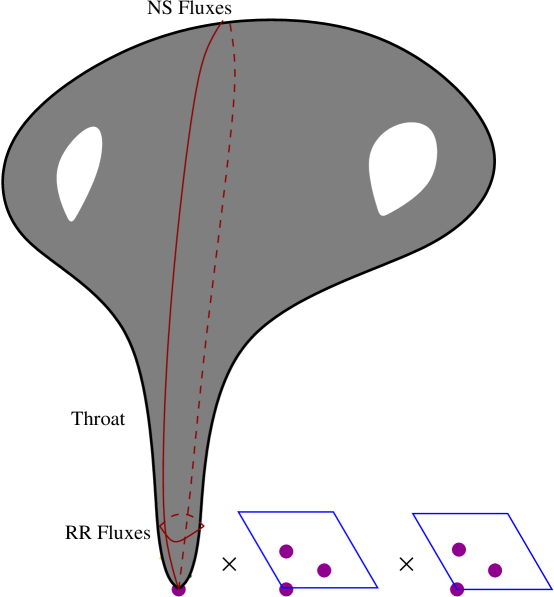
Figure 1: Description of a warped throat with 3-form fluxes embedded in a compact geometry, with anti-D3-branes trapped at the tip of the throat. At the tip of the throat there is also a twisted $T^{4}$ with the 9 fixed points under a ${\mathbb{Z}}_{3}$ symmetry indicated. D7 branes can wrap 4-cycles outside the throat and/or the $T^{4}$ in the tip of the throat, (anti) D3 branes live at the fixed points.

The presence of these fixed points has several consequences. First, the various tadpole conditions imply the existence of chiral fields and gauge interactions on the branes localized at the fixed-points, and these can contain gauge groups and matter fields which contain the Standard Model spectrum [37]. They also potentially introduce new moduli corresponding to the blowing-up mode, $b$, for each of the corresponding singularities. Therefore, even if we follow IKLT by starting with a model with all complex structure moduli fixed by fluxes and having only a single Kähler modulus which is fixed by nonperturbative effects associated with D7 branes away from the throat, having new fixed points introduces new moduli whose stabilization must be addressed.

As it happens, these new moduli generally do appear in the low-energy supergravity potential, in the form of a $D$-term. They typically do so because supersymmetry pairs the blowing-up modes with axion fields, $\beta$, which are required to cancel the anomalies which the chiral fermions of the low-energy theory have for various $U(1)$ gauge groups. To see why this is so, notice that anomaly cancellation requires the axion field to have both of the couplings $\partial_{\mu}\beta\,A^{\mu}$ and $\beta\,F_{\mu\nu}\widetilde{F}^{\mu\nu}$, where $F=dA$ is the gauge field for the anomalous $U(1)$. But supersymmetry in 4D then relates these two couplings to others involving the blowing up modes. In terms of the chiral scalar, $B=b+i\beta$, containing both the axion and the blowing up mode, anomaly cancellation requires the following two couplings [38].

• The coupling $\beta\,F_{\mu\nu}\widetilde{F}^{\mu\nu}$ requires the holomorphic gauge coupling function must depend on $B$, according to

  $$f=f_{0}+\alpha B$$ (15)

  for some nonzero constant $\alpha$. The form for $f_{0}$ depends on the origin of the anomalous $U(1)$. If it is associated with a D7 brane which lies far from the throat, then $f_{0}=T$ as was the case for the gaugino condensation within the IKLT framework. On the other hand, if the anomalous $U(1)$ arises from a D7 brane located at the tip of the throat then the gauge coupling function goes like $L^{4}/z_{0}^{2}$, and so the warping cancels the $L$ dependence, leading to a $T$-independent result: $f_{0}=S=$ (constant). A $T$-independent gauge coupling function is also what is expected if the anomalous $U(1)$ is associated with a D3 brane situated anywhere within the internal 6 dimensions.

• The $\partial_{\mu}\beta A^{\mu}$ term requires the chiral scalar $B$ can only appear in the Kähler potential together with the anomalous $U(1)$ gauge multiplet, $A$, through the combination $B+B^{*}+A$. This in turn implies the existence of a Fayet-Iliopoulos $D$-term [40] proportional to $\partial K/\partial B$.

Using these in the 4D supergravity action (and expanding the Kähler function to leading order in powers of the chiral matter fields, $Q$) leads to a contribution to the low-energy 4D scalar potential for $B$ having the $D$-term form:

$$V_{D}=g^{2}\left[\left(\frac{\partial K}{\partial B}\right)_{A=0}-Q^{\dagger}qQ\right]^{2}\,,$$ (16)

where $g^{-2}=f+f^{*}$ is the inverse 4D gauge coupling for the anomalous $U(1)$. Here $q$ generically denotes the charge matrix of the chiral matter fields under the anomalous $U(1)$. Clearly this potential generically lifts the flat directions associated with $B$, as does gaugino condensation by any nonabelian gauge-group factors for which the gauge coupling function is given by eq. (15).

3 The Effective Theory

With an eye to searching for inflation, in this section we write down a four dimensional effective field theory which is meant to capture the low-energy dynamics of a mobile D3 brane moving within the string vacua discussed above (and hopefully for more general configurations). To this end we include in the low energy theory representatives of each of the types of moduli described in the previous section as well as the position modulus of the mobile D3 brane. Our goal is to follow the way that the mobile brane and other moduli move under the influence of the geometry and forces due to the other branes.

Thus, we choose a Lagrangian which depends on the following fields: (1) the moduli $T$ and $B$; (2) various gauge multiplets, including at least one anomalous $U(1)$ multiplet, $A$; (3) the chiral matter fields, $Q$, whose fermions are responsible for the $U(1)$ anomalies; and (4) the position modulus, $\phi$, of the D3 brane whose motion is the putative inflaton. If we were to set the fields $A$, $B$ and $Q$ to zero, we would be left with a Lagrangian only for the fields $T$ and $\phi$ for which the analysis of [9] applies (and shows that inflation is not easily generated). In this sense our scenario generalises the one in [9]. For simplicity of analysis we specialize to the case of a single anomalous $U(1)$ multiplet, $A$, to a single charged field, $Q$, and to a single modulus, $B$, but we expect our results to also apply to the more realistic case where several such moduli appear.

We next discuss in turn the supersymmetric and nonsupersymmetric contributions to the low-energy scalar potential.

3.1 Supersymmetric Terms

We imagine the gauge group of the low-energy theory to include unbroken nonabelian factors associated with some of the D7 and D3 branes of the model, and that these gauge interactions confine at energies below the compactification scale. We further imagine some of the relevant D7 branes are located far from the throat, and so have gauge coupling functions ${\cal F}_{ab}=({\cal F}_{0}+T)\delta_{ab}$. We also assume there to be a nonabelian gauge group associated with the branes which are localized at the orbifold points, and that these are located at the throat’s tip and so have gauge coupling functions of the form ${\cal F}^{t}_{ab}=({\cal F}^{t}_{0}+B)\delta_{ab}$. As discussed above, in these expressions ${\cal F}_{0}$ and ${\cal F}^{t}_{0}$ are constants which are independent of the low-energy moduli of interest.

These nonabelian gauge groups are assumed to exist in addition to the anomalous $U(1)$ gauge group mentioned above, whose gauge fields survive into the low-energy theory. Since this $U(1)$ is assumed to be associated with a brane at the throat’s tip, its low-energy gauge coupling function, $f$, is independent of $T$. $f$ must depend on $B$, however, since this is required by the condition that Im$B$ cancel the $U(1)$ anomalies in the low-energy theory.

Since our interest is in the effective theory below the condensation scale for the nonabelian gauge groups, their gauge degrees of freedom can be integrated out. Their sole low-energy influence is then through the nonperturbative effects to which they give rise (like gaugino condensation [23, 24]) since these generate contributions to the low-energy superpotential of the form $W_{np}=A\,e^{-aT}+C\,Q^{\ell}\,e^{-cB}$. (The power, $\ell$, of $Q$ which appears here is determined by the condition that $W_{np}$ be invariant under the gauged $U(1)$ symmetry, under which Im$B$ shifts like a would-be Goldstone boson.) In general the quantities $A$ and $C$ could also depend on other moduli, such as $\phi$ [9, 34], but this dependence need not be strong, particularly if the mobile D3 brane should be distant from the brane on which the condensation occurs. We do not use this $\phi$ dependence in what follows.

We are led in this way to describing the supersymmetric part of the low-energy theory (below the confinement scale of the nonabelian gauge bosons) by a 4D supergravity model which is characterized by the following Kähler function, $K$, superpotential, $W$, and $U(1)$ gauge coupling function, $f$:

$$K = -3\,\ln r+{\cal B}\left(B+B^{*}+A\right)+{{\cal Q}}\left(Q^{\dagger}\,e^{A},Q\right)$$

$$f = f_{0}+\alpha\,B\qquad\hbox{and}\qquad W=w+W_{p}(Q)+W_{np}(T,B)\,.$$ (17)

Here ${\cal B}$ and ${\cal Q}$ are arbitrary real functions of their arguments, and $w$ is the term in the superpotential which arises in the low-energy theory due to the fluxes which fix the complex-structure moduli. We follow IKLIMT by taking $w$ to be independent of $T$, $\phi$ and $B$, and by taking $r=T+T^{*}-k(\phi^{*},\phi)$ [30, 9], with the logarithm expressing the leading dependence of $K$ on $T$ and $\phi$ for large $r$. The function $k(\phi,\phi^{*})$ is the Kähler potential for the underlying metric on the internal Calabi-Yau space itself. As discussed above, the quantity $f_{0}$ is a constant if the anomalous $U(1)$ is associated with a D3 brane, or for a D7 brane localized at the throat’s tip. For D7’s located elsewhere we instead have $f_{0}$ proportional to $T$ which was used to induce the nonperturbative dependence on $T$ of $W$. Finally, we include a perturbative superpotential, $W_{p}(Q)$, since in general charged matter fields acquire cubic tree-level superpotentials in the low-energy theory.

The contributions of $r$ and $B$ to the Kähler function arise as a sum of contributions as written above since microscopically the $B$’s are associated with fixed points while $T$ and $\phi$ are not. (A similar split would also have occurred if $B$ had been an unfixed complex-structure modulus.) Similar remarks apply to the dependence of $K$ on $Q$, but this does not significantly influence our results. With these choices the kinetic energies for the fields are controlled by the following Kähler metric

$$ds^{2} = \frac{3}{r^{2}}\Bigl{[}dT^{*}dT+\left(r\,k_{\phi\phi^{*}}+k_{\phi}\,k_{\phi^{*}}\right)d\phi^{*}d\phi-\left(k_{\phi}\,dT^{*}d\phi+\hbox{c.c.}\right)\Bigr{]}$$ (18)

$$\qquad\qquad\qquad+{\cal B}^{\prime\prime}\,dB^{*}dB+{\cal Q}_{Q{Q}^{*}}\,d{Q}^{*}dQ\,,$$

where for simplicity we restrict to a single charged chiral field, $Q$. As usual subscripts denote differentiation with respect to the appropriate fields, and primes denote differentiation with respect to the function’s argument.

The $D$-term and $F$-term contributions to the scalar potential $V=V_{F}+V_{D}$ for such a supergravity become

$$V_{D}=\frac{({\cal B}^{\prime}+q{\cal Q}_{\overline{Q}}Q)^{2}}{f+f^{*}}=\frac{({\cal B}^{\prime}+q{\cal Q}_{\overline{Q}}Q)^{2}}{f_{0}+f_{0}^{*}+\alpha(B+B^{*})}\,,$$ (19)

and

$$V_{F} = \frac{e^{{\cal B}+{\cal Q}}}{r^{3}}\left[\frac{r^{2}\left|W_{T}\right|^{2}}{3}\left(1+\frac{k_{\phi}k_{\phi^{*}}}{rk_{\phi\phi^{*}}}\right)-r\,\Bigl{(}W^{*}W_{T}+\hbox{c.c.}\Bigr{)}\right.$$

$$\qquad\qquad+\left.\frac{\left|W_{B}+{\cal B}^{\prime}\,W\right|^{2}}{{\cal B}^{\prime\prime}}+\frac{\left|W_{Q}+{\cal Q}_{Q}\,W\right|^{2}}{{\cal Q}_{Q\overline{Q}}}\right]\,.$$

3.2 Supersymmetry-Breaking Terms

Because the realistic models typically involve both branes and antibranes, for the antibranes supersymmetry is broken at the scale of the brane tension (i.e. the string scale, modified by the warp factor appropriate to the brane position). Consequently, in addition to the previous supergravity Lagrangian we must also include in the low-energy theory terms which explicitly break supersymmetry.

Although a general statement of the low-energy form of the Lagrangian for branes interacting with antibranes is not yet known [29], approximate expressions may be obtained in the limit that the antibrane supersymmetry-breaking effects are perturbatively small. In this limit their leading effects may be added to the supergravity Lagrangian considered above. We obtain then the low-energy 4D scalar potential $V=V_{F}+V_{D}+V_{sb}$ with $V_{F}$ and $V_{D}$ given as above, and where $V_{sb}$ can also be written as a sum of two terms: the antibrane’s tension term plus a brane-antibrane interaction term, $V_{sb}=V_{T}+V_{int}$. We expect the supersymmetry breaking also introduces the soft susy-breaking terms, $V_{soft}$, including trilinear terms and scalar masses for matter fields, which the low-energy phenomenology of the $Q$ fields would require.

The tension part of the supersymmetry-breaking potential takes the form

$$V_{T}=\frac{k}{r^{2}}\,,$$ (21)

which is the IKLT result for antibranes localized near the tip of the throat. Recall that if the supersymmetry breaking is due to anti-D3 branes, then $k$ is related to the brane tension $T_{3}$ by $k=2z_{b}^{2}T_{3}/g_{s}^{4}$.

As before, the brane-antibrane interaction term similarly is given by

$$V_{int}=\frac{k^{\prime}}{r^{2}}\,G(\phi,\phi_{0})$$ (22)

where $\phi_{0}$ denotes the coordinate position of the antibrane. In what follows we shall use the explicit expression

$$G\propto\frac{1}{(\psi-\psi_{0})^{4}}\,,$$ (23)

with the real coordinate $\psi$ representing the position of the mobile brane and $\psi_{0}$ denoting the antibrane position in the same coordinates. This expression follows quite generally if the proper separation between the brane and antibrane is very small compared with the geometry’s radius of curvature, since in this case $G\propto s^{-4}$ and $s^{2}\approx\sum_{i}|\phi^{i}-\phi_{0}^{i}|^{2}$. The above expression then follows provided we choose $\psi^{2}=\sum_{i}|\phi^{i}|^{2}$, and minimize over the directional variables of $\phi^{i}$.

Alternatively, eq. (23) also follows if the antibranes are at the throat’s tip, with the mobile brane also within the throat. This follows if we work in the coordinates defined by the metric of eq. (14), and choose $\psi=\psi_{0}+r$.

4 Inflationary Dynamics

In this section we explore the dynamics which is implied by the above 4D effective theory, with the goal of identifying the circumstances under which it permits an inflationary slow roll, given that all of the potential moduli are left free to move. We do find that inflation is generically difficult to obtain (in agreement with [9]), and we find that this property is not significantly changed by the presence of new moduli like $B$ in our model. Unlike these authors we explicitly identify some of the special circumstances which do allow inflation, in order to see how unusual inflationary solutions are. We also identify in this section the observational consequences which follow from the inflationary trajectories which we do find.

4.1 Domain of Validity of Approximations

Before presenting numerical results, we briefly pause to describe some preliminary considerations which are useful to have in mind when performing the detailed analysis. Because our scalar fields have nonminimal kinetic terms, the scalar parts of our low-energy effective actions have the generic form

$${S}_{\rm scalar}=-\int d^{4}x\;\sqrt{-g}\left[\,\frac{1}{2}\,g_{ij}\,\partial_{\mu}\varphi^{i}\,\partial^{\mu}\varphi^{j}+V(\varphi)\right]\,,$$ (24)

with the target-space metric, $g_{ij}$, given by eq. (18) and the scalar potential, $V$, as discussed at length in previous sections. The field equations which follow from this Lagrangian density are

$$\ddot{\varphi}^{i} + 3H\dot{\varphi}^{i}+\Gamma^{i}_{jk}\,\dot{\varphi}^{j}\,\dot{\varphi}^{k}+g^{ij}\,{\partial V\over\partial\varphi^{j}}=0\,,$$

$$H^{2} = \left({\dot{a}\over a}\right)^{2}={8\pi G\over 3}\left(\frac{1}{2}g_{ij}\dot{\varphi}^{i}\dot{\varphi}^{j}+V\right)\,,$$ (25)

where $a$ is the scale factor for the 4D FRW metric, dots denote time derivatives and the $\Gamma^{k}_{ij}$ denote the target-space Christoffel symbols constructed using the metric $g_{ij}$. Notice that the new terms involving the Christoffel symbol in the scalar field equation are quadratic in time derivatives, and so are normally negligible in the slow-roll approximation. Even so, in later sections we integrate the full equations when numerically computing scalar evolution.

Because of the nontrivial target-space metric we must adopt slow-roll criteria which differ slightly from those normally used. An invariant notion of the slowness of the scalar evolution is controlled by the smallness of the generalized slow-roll parameters defined by $\epsilon$ and $\eta=\hbox{min}_{a}\,\eta_{a}$, where

$$\epsilon=\frac{M_{p}^{2}}{2}\,g^{ij}\left(\frac{V_{i}\,V_{j}}{V^{2}}\right)\qquad\hbox{and}\qquad{N_{i}}^{j}v^{(a)}_{j}=\eta_{a}\,v^{(a)}_{i}\,.$$ (26)

Here $V_{i}=\partial_{i}V=\partial V/\partial\varphi^{i}$ and the $\eta_{a}$ are eigenvalues of the matrix, ${N_{i}}^{j}=M_{p}^{2}\,g^{jk}\,V_{;ik}/V$. The target-space covariant derivative is built in the usual way from the target-space Christoffel symbols: $V_{;ij}=\partial_{i}\partial_{j}V-\Gamma^{k}_{ij}\partial_{k}V$. These expressions agree with the usual ones when $g_{ij}=\delta_{ij}$, and are invariant under scalar field redefinitions.

A second general consideration involves the domain of validity of the low-energy effective theory. In particular, the derivation of the form of the 4D Lagrangian for the moduli presupposes the internal dimensions to be much larger than the string scale. In 4D Planck units this requires $r,\sigma\gg 1$. Since it is more convenient numerically to deal with fields which are $O(1)$, many of the solutions we find also have $r\sim\sigma\sim O(1)$. We therefore return at the end of the next section to show how to construct solutions having larger values of $r$ and $\sigma$ from the ones we present numerically.

4.2 Inflationary Dynamics

We now describe our numerical results which explore the inflationary possibilities of our effective 4D theory in more detail. These results were obtained by numerically evolving the scale factor, $a$, of the 4D metric and all of the scalar moduli forward in time, starting from rest, using the full equations, (4.1). In practice this is most easily done by using the scale factor itself as the time variable when integrating the scalar field equations.

The scalar fields whose evolution we follow are the complex quantities $T=\frac{1}{2}\,\sigma+i\tau$, $B=b+i\beta$, $Q$ and $\phi^{i}$, with $i=1,2,3$. The numerical evolution we describe was performed using the target-space metric defined by eq. (18), such as follows for the scalar part of the 4D supergravity defined by the functions $K$, $f$ and $W$ of eqs. (3.1). For simplicity we take the function ${\cal B}$ to be ${\cal B}=\frac{1}{2}\,(B+B^{*})^{2}$, and approximate the Calabi-Yau Kähler function by $k(\phi^{*},\phi)=\sum_{i}|\phi^{i}|^{2}$. We take the scalar potential to be the sum of $V_{D}$, $V_{F}$, $V_{T}$ and $V_{\rm int}$, as given by eqs. (19), (3.1), (21) and (22).

4.2.1 Qualitative Description

Although our full numerical simulations follow all of the moduli, for the inflationary solutions we present, none of the fields are very important besides the two fields $\sigma=2\hbox{Re}\,T$ and the brane position, $\psi^{2}=\sum|\phi^{i}|^{2}$, (whose relation to coordinates on the Calabi-Yau space is given below eq. (23)). This is because for these solutions the other fields tend to roll quickly to the local $\sigma$- and $\psi$-dependent minima of their potentials, leaving the long-term behaviour dominated by the $\sigma$ and $\psi$ evolution. It is therefore instructive to approximately integrate out these other fields analytically in order to understand qualitatively the potential which governs the inflationary dynamics. This is the topic of the present section.

The field $Q$ generally likes to very quickly sit at its minimum, and so does not contribute to the scalar dynamics in an interesting way. In what follows all we need to know about this minimum is that it occurs at nonzero $Q$. This would automatically be preferred if the power of $Q$ in the superpotential $Q^{\ell}\,e^{-cB}$ were to satisfy $\ell\leq 1$. The stabilization of $Q$ away from zero is automatic if $\ell<1$ since in this case $\partial W/\partial Q$ involves negative powers of $Q$, which drive the field away from zero. It is then stabilized at a finite value because positive powers of $Q$ appearing in the Käher function also prevent a runaway to infinity. Alternatively, stabilization of $Q$ away from zero might also be arranged by suitably designing the interactions of the perturbative superpotential, $W_{p}$, or the $Q$-dependent soft supersymmetry-breaking terms.

It is very simple to analytically integrate out the imaginary parts of $T$ and $B$. With the assumption $k(\phi^{*},\phi)=\sum_{i}|\phi^{i}|^{2}=\psi^{2}$, only $V_{\rm int}$ cares about the direction, $\theta$, of $\phi^{i}$, and this (for real $\phi_{0}$) is minimized by setting all components of $\phi^{i}$ to zero apart from the overall modulus $\psi$. Once this is done we have $r=\sigma-\psi^{2}$. It is only $V_{F}$ which depends on Im$T=\tau$ and Im$B=\beta$, with

$$V_{F} = {e^{2b^{2}}\over r^{3}}\left(2\,{\frac{AC\left(ra+4\,{b}^{2}-2\,cb\right)\cos\left(\tau-\beta\right)}{{e^{a\sigma/2}}{e^{cb}}}}+2\,{\frac{Aw\left(ra+4\,{b}^{2}\right)\cos\tau}{{e^{a\sigma/2}}}}\right.$$

$$+ 4\,{\frac{bCw\left(2\,b-c\right)\cos\beta}{{e^{cb}}}}\left.+{\frac{{A}^{2}\left(12\,{b}^{2}+6\,ra+r\sigma\,{a}^{2}\right)}{3{e^{a\sigma}}}}+{\frac{{C}^{2}\left(2\,b-c\right)^{2}}{\left({e^{cb}}\right)^{2}}}+4\,{b}^{2}{w}^{2}\right)$$

where $A$, $a$, $C$, $c$ and $w$ are the constants which appear in the superpotential (after the vacuum value of $Q$ is absorbed),

$$W=w+A\,e^{-aT}+C\,e^{-cB}\,,$$ (28)

which we take to be real and positive. Minimizing with respect to $\tau$ and $\beta$, we find that $w\cos\tau=-|w|$ at the minimum, and $\beta=0$.

To minimize with respect to $B$, we can use the hindsight that $B$ typically evolves toward small field values, since it is only the exponential superpotential, $Ce^{-cB}$, which excludes the solution $B=0$. For small $B$ we can take the gauge kinetic function to be a real constant, $f=f_{0}$, without loss of generality, and so $V_{D}=2|B|^{2}/f_{0}$. For small $B$, $V_{F}$ can be approximated by expanding to quadratic order in $B$, giving

$$V(B)\cong\alpha+\beta B+\frac{1}{2}\gamma B^{2}\,,$$ (29)

where $\alpha$, $\beta$ and $\gamma$ are calculable functions of $r$ and $\sigma$. The value of $B$ which minimizes the potential is then $B=-\beta/\gamma$, and the value of the potential at this minimum is $V_{\rm min}=\alpha-{\beta^{2}/2\gamma}$. We have verified that this actually gives a quite good approximation to the full $B$-dependent potential once $B$ has settled down to its instantaneous local minimum, due to the Hubble damping of its oscillations during inflation.

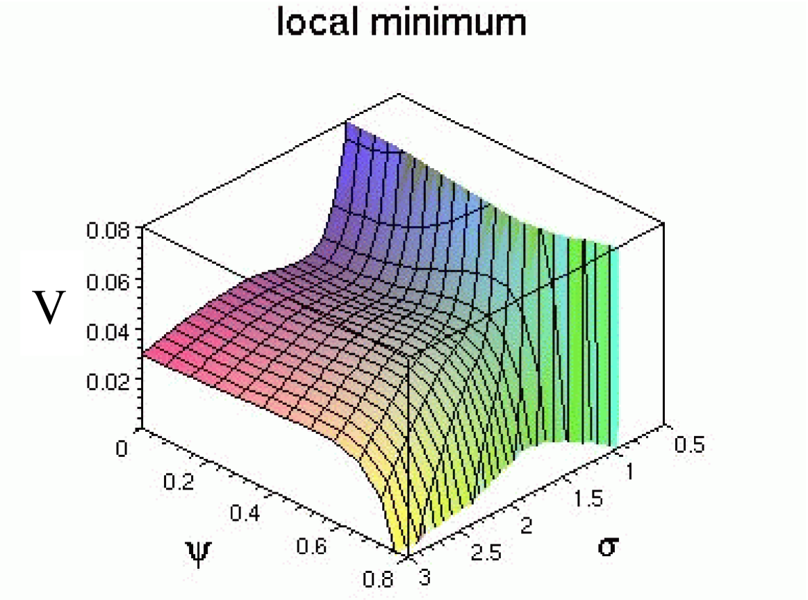
Figure 2: The potential with a local minimum in the trough, which leads to old inflation.

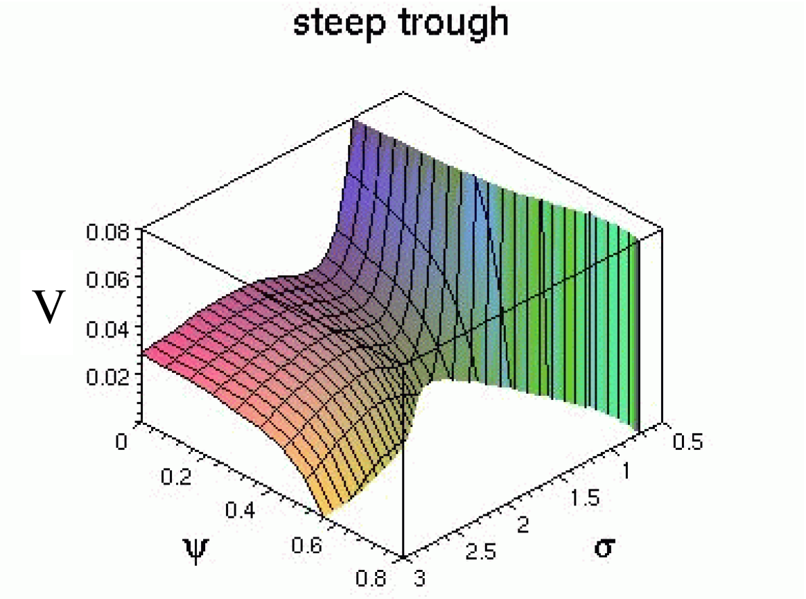
Figure 3: The potential with a steep trough, which gives a short period of inflation.

Given these values for the other moduli, we may now examine the potential $V=V_{D}+V_{F}+V_{sb}$ as a function of $\sigma$ and $\psi$ to discover the conditions that will lead to inflation, typically with $\psi$ playing the role of the inflaton. The parameter space for the full potential is large, consisting of $A,a,C,c,k,k^{\prime},f_{0},\psi_{0}$, where $\psi_{0}=|\phi_{0}|$ is the modulus of the antibrane position (see (22) and the discussion following).

Despite the large number of parameters which can be varied, we find essentially one situation where inflation can occur. For certain parameter values, a trough can form along the $\psi$ direction, as shown in Figs. 3 and 3. This trough can have a local minimum at small values of $\psi$, as in Fig. 3, or else it slopes monotonically toward zero potential, in the direction of the brane-antibrane annihilation, as in Fig. 3. The parameters chosen to obtain these figures are

$$w=0.25,\ {f_{0}}=1.175,{A}=0.9,\ a=2.1,\ {C}=0.51,\ c=1,\ k=0.3,\ {\psi_{0}}=1.136$$ (30)

with $k^{\prime}=0.005$ chosen for Fig. 3 and $k^{\prime}=0.03$ for Fig. 3. (Recall that these values are expressed in 4D Planck units, with $M_{p}=(8\pi G)^{-1/2}=1$.)

The qualitative features of this potential can be understood as follows:

• The function $\alpha$ in (29) has the form

  $$\alpha(\sigma,\psi)={\frac{\left(2\,a+\sigma\,{a}^{2}/3\right){{A}}^{2}}{{r}^{2}{e^{a\sigma}}}}-{\frac{\left(2\,wa+2\,{C}\,a\right){A}}{{r}^{2}{e^{a\sigma/2}}}}+{\frac{{{C}}^{2}{c}^{2}}{{r}^{3}}}\,.$$ (31)

  For the chosen parameters, $\alpha$ has a minimum as a function of $\sigma$ over the interesting range of $\psi$. This explains the existence of a trough in the $\psi$ direction. Furthermore, the correction $-\beta^{2}/(2\gamma)$ in (29) does not destroy this trough. The minimum with respect to $\sigma$ is a consequence of the usual modulus stabilization due to gaugino condensation. It is only a local minimum; for larger values of $\sigma$, there is runaway behavior toward $\sigma\to\infty$.

• The behavior in the $\psi$ direction depends not only on $\alpha$ but also the SUSY-breaking terms in the potential, whose strengths are determined by $k$ and $k^{\prime}$. For example a function of the form $k_{0}r^{-n}-k^{\prime}r^{-2}(\psi-\psi_{0})^{-4}$ (where the first term represents the typical dependence on $\psi$ of the F-term contributions to the potential) can be seen to have the observed qualitative behavior of $V(\psi)$ along the trough for fixed $\sigma$. Whether there is a saddle point along the trough is controlled by the relative sizes of the parameters $k_{0}$, $k^{\prime}$ and $\psi_{0}$. The runaway to large $\psi$ arises once the brane-antibrane attraction dominates, and describes the approach of these two objects in prelude to their mutual annihilation.

In the case where there is a local minimum in the trough, as shown in Fig. 3, a de Sitter solution may be obtained along the lines of that obtained in ref. [11] simply by sitting at the local minimum, provided that the parameters are chosen to ensure the potential is positive there. Of course this provides at best an example of old inflation, in which most of the universe continues to inflate forever, and so is not a phenomenologically attractive scenario. But it is possible to obtain inflation by tuning away the local minimum and so flattening the trough. Since, generically, the curvature of the saddle point which separates the local minimum from the large-$\psi$ region is a function of all these parameters,

$$\left.{\partial^{2}V\over\partial\psi^{2}}\right|_{\rm saddle\ pt.}=f(A,a,C,c,k,k^{\prime},f_{0},\psi_{0}),$$ (32)

sufficient flatness — i.e., $({\partial^{2}V/\partial\psi^{2}})|_{s.p.}=0$ — can be obtained by adjusting practically any of the parameters in $V$. This highly tuned situation is the optimal one for inflation, since going beyond it to negative values of $({\partial^{2}V/\partial\psi^{2}})$ leads to a steeper trough, and so leads to an earlier end for inflation, with typically far less than the canonical 60 $e$-foldings of inflation.

4.2.2 Numerical Results

We now report on the results of the full numerical evolution of all of the scalar moduli, using the full equations of motion, eqs. (4.1).

We have explored the sensitivity of the duration of inflation to the parameter values, and find that in order to get 60 $e$-foldings, a tuning of 1 part in 1000 is required in any given parameter. If we tune to only a part in 100, as might have been naively expected to suffice, we obtain only about 30 $e$-foldings. The situation is illustrated with respect to the parameters $k^{\prime}$ and $k$, which appear in the SUSY-breaking part of the potential, in Figs. 5 and 5. It is worth remarking that a small number of $e$-foldings like 30 could be phenomenologically viable if the mechanism of reheating were inefficient enough to give a reheat temperature far below the string scale [44]. Such a possibility is not out of the question, since the mechanism of reheating after brane-antibrane annihilation is unknown. If, for instance, the false vacuum energy were initially dumped mainly into invisible closed-string modes, the reheat temperature in visible radiation could naturally be small.

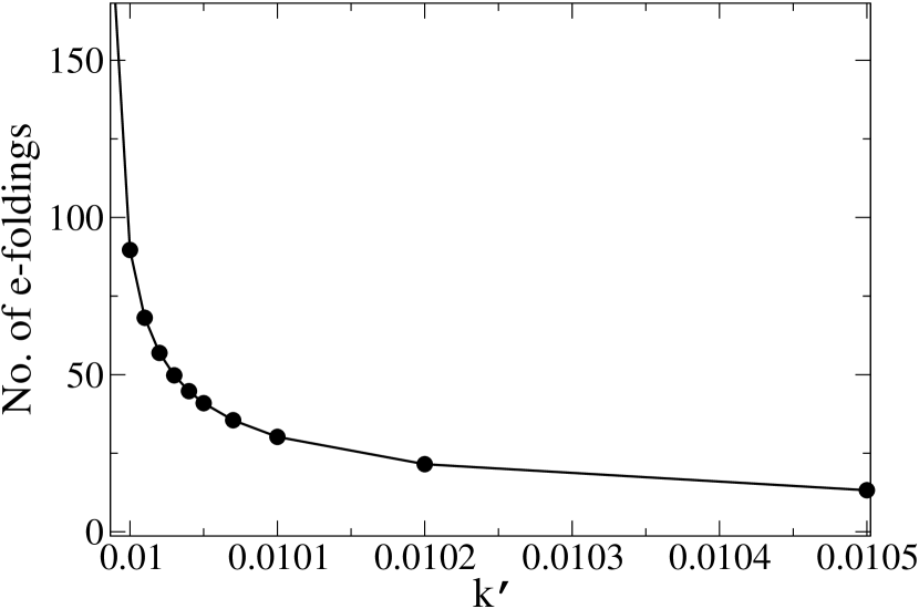
Figure 4: Dependence of the amount of inflation on the value of the brane-antibrane interaction strength $k^{\prime}$.

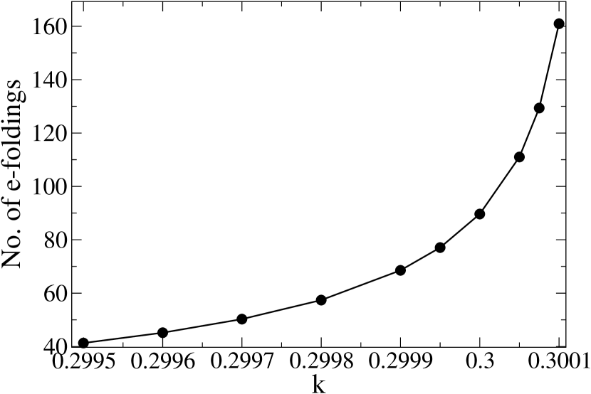
Figure 5: Dependence of the amount of inflation on the tension parameter $k$ in the SUSY-breaking part of the potential.

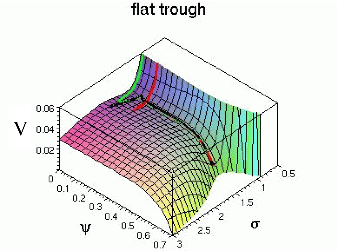
Figure 6: Potential with a flat trough, showing several inflaton trajectories starting from different initial field values. Parameters are given by eq. (4.7) and $k^{\prime}=0.01$.

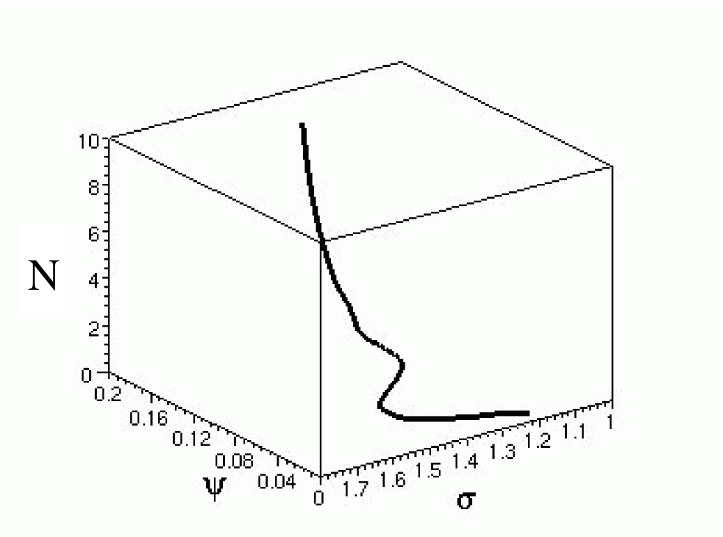
Figure 7: The first 10 (out of 90) $e$-foldings of expansion as a function of evolving field values for one of the trajectories in Fig. 6.

Fig. 7 shows several trajectories for the fields $\{\sigma,\psi\}$, starting initially at rest, drawn on their potential in the case where the trough is sufficiently flat to yield up to 90 $e$-foldings of inflation. (With a finer tuning of parameters, even more inflation is possible; this example uses the parameters in (30) and $k^{\prime}=0.01$.) The trajectories are integrated until the potential becomes negative; at this point the brane and antibrane are close to annihilating, and we expect that the low-energy effective action no longer gives an accurate description of the system, due to large corrections at the string scale.

In contrast to the precision of the tuning required for the parameters of the potential in order to obtain a flat enough potential, the sensitivity to the initial conditions of the inflaton moving in this potential is quite mild. The fields quickly roll to the trough, within the first $2$-$3$ $e$-foldings of expansion, as illustrated in Fig. 7. The total amount of inflation obtained is controlled mainly by the initial value of $\psi$, which determines how much of the trough is traversed. Fig. 9 shows the number of $e$-foldings which are achieved as a function of initial field values.

For completeness, we also illustrate the evolution of $B$ during inflation along the trough in Fig. 9. This figure shows that the initial transient oscillations die out within the first 4 $e$-foldings, and $B$ remains nearly constant during the slow-roll period. Furthermore, its small value during this roll justifies the heuristic use of a Taylor expansion in $B$ of the full potential, which we employed for the qualitative description given above.

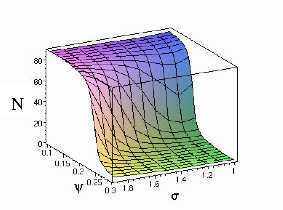
Figure 8: The number of $e$-foldings of expansion as a function of initial field values for the potential in Fig. 6

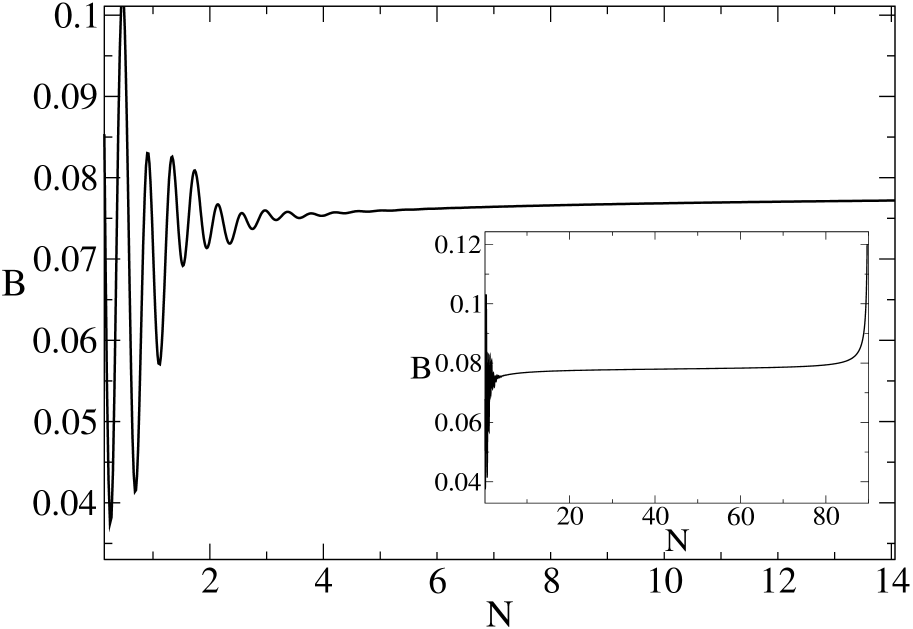
Figure 9: Evolution of the $B$ field for a typical trajectory, at early times. Inset shows the evolution over the entirety of inflation.

Multi-Field Inflation: One might ask whether $\psi$ need always be the inflaton, or whether instead $\sigma$ could play this role. If so it might be possible to take advantage of the arguments of ref. [3] that under certain circumstances a radion such as $\sigma$ can have a naturally very slow roll. It is also worth searching for inflationary trajectories where both fields roll, since these can give rise to observable signals for the Cosmic Microwave Background (CMB), such as isocurvature density perturbations.

We did not find any examples of radion inflation, but did find some inflationary trajectories along which both $\sigma$ and $\psi$ rolled appreciably. For these alternative solutions a hole can be opened along the side of the trough, allowing the fields to escape in the direction of increasing $\sigma$, before finally veering in the direction of brane-antibrane annihilation. The situation is illustrated in Figs. 11 and 11. This behaviour is obtained by lowering the value of $A$ to 0.897, while keeping other parameters of (30) fixed. Successful inflationary trajectories loiter at some place in the trough during most of inflation, before eventually leaving it in the $\sigma$ direction. At the very end of inflation $\psi$ once again takes over the motion and the annihilation of brane and antibrane takes place. The twisted nature of the field-space trajectories is shown in Fig. 13 (and in a projected view in Fig. 13), which illustrates the evolution of the fields as a function of the expansion. It is possible to have periods during which the trajectories curve significantly, which could have observable consequences for density perturbations, as we will discuss below.

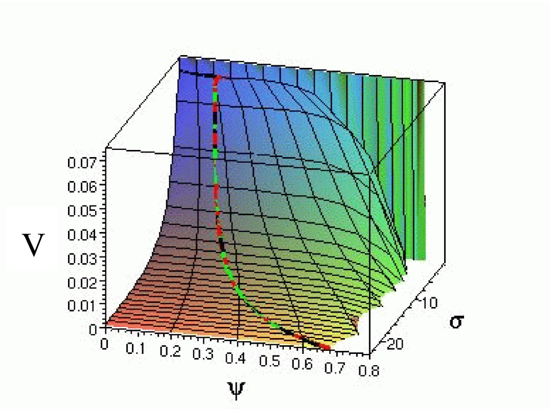
Figure 10: Potential with an opening in the trough, showing several inflaton trajectories.

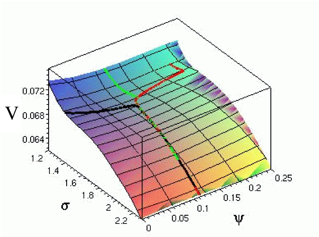
Figure 11: Closeup of the trough region in figure 10.

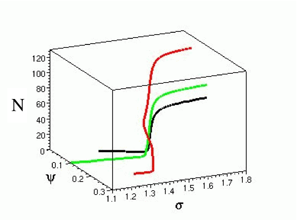
Figure 12: The number of $e$-foldings versus field values for the three trajectories shown in figures 10 and 11.

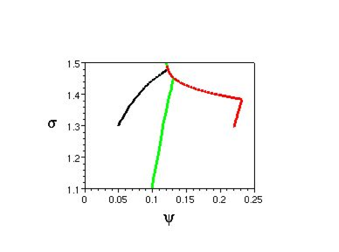
Figure 13: Projection of previous figure on the $\psi$-$\sigma$ plane.

4.2.3 Scaling Arguments

The previous examples use a numerically convenient choice of model parameters which are $O(1)$ in Planck units. We return now to the issue of whether these solutions lie within the domain of validity of the low-energy field theory, which require $r,\sigma\gg 1$. We do so by identifying two separate scaling symmetries which the solutions to the scalar equations approximately enjoy when they are in the slow-roll limit.

There is a scale invariance satisfied by any scalar potential in the slow-roll approximation, and so which holds throughout almost the entirety of inflation. This symmetry follows because the slow-roll equations are unchanged under an overall rescaling of the potential, $V\to\lambda V$, accompanied by a rescaling of time, $t\to t/\sqrt{\lambda}$. Under such a change, the slow-roll equations transform as

$$H={\dot{a}\over a}=\sqrt{V/3}\ \to \ H=\sqrt{\lambda}\,{\dot{a}\over a}=\sqrt{\lambda V/3};$$

$$3H\dot{\phi}^{i}=-V^{,i}\ \to \ 3\sqrt{\lambda}H\sqrt{\lambda}\dot{\phi}^{i}=-\lambda V^{,i}$$ (33)

Although the time-dependence of solutions is stretched by this transformation, the number of $e$-foldings is unchanged and so there is no change at all in the solutions for the field equations if it is the number of $e$-foldings, $u\equiv\ln a$, which is used as the independent variable, $\phi=\phi^{i}(u)$.

In the present instance this rescaling is accomplished by letting the Lagrangian parameters scale as,

$$\{A,C,w\}\to\sqrt{\lambda}\{A,C,w\},\quad\{k,k^{\prime},1/f_{0}\}\to\lambda\{k,k^{\prime},1/f_{0}\}\,,$$ (34)

which simply corresponds to changing the string scale (in Planck units). Of course, the freedom to choose this scale is lost once we demand to reproduce the observed magnitude of the density perturbations in the CMB, as is done below.

There is a slightly more subtle rescaling property of the solutions considered here, which has important implications for the validity of our approximations. In the slow-roll limit, our scalar equations are unaffected by the transformation:

$$a\to\lambda^{\prime}a,\quad\{\sigma,\psi^{2},\psi_{0}^{2}\}\to\{\sigma,\psi^{2},\psi_{0}^{2}\}/\lambda^{\prime},\quad k^{\prime}\to k^{\prime}/\lambda^{\prime 2}\,,$$ (35)

which gives an overall rescaling $V\to\lambda^{\prime 2}V$, but without rescaling the time coordinate. This rescaling to $V$ could be undone by a transformation of the type (34) if desired, but we instead use it to generate new solutions for which $\psi$ and $\sigma$ are larger, since $r\to r/\lambda^{\prime}$. That is, given any parameter set which leads to a successful inflationary slow roll, a continuous family of solutions can be constructed that leads to the same physical predictions, while ensuring that $r$ is in the range where the effective theory is trustworthy.

4.3 Density Perturbations

It is natural to ask for the observable implications of the inflationary solutions just discussed, so we now calculate the signature of fluctuations which they predict for the temperature of the cosmic microwave background (CMB). The precise expression for the power spectrum in a multi-field inflationary model can be written as

$$P(k)={8\pi G\,V\over 75\pi^{2}}\,g^{ij}\,{\partial N\over\partial\phi^{i}}{\partial N\over\partial\phi^{j}}$$ (36)

(in the notation of [45], $P(k)=\delta_{H}^{2}$), where the COBE normalization implies that $\sqrt{P(k_{0})}=2\times 10^{-5}$ at the scale $k_{0}\sim 10^{3}$ Mpc.

We find that in the present model, the exact power spectrum is well approximated by the computationally simpler formula

$$P(k)={3\over 75\pi^{2}}{H^{4}\over g_{ij}\dot{\phi}^{i}\dot{\phi}^{j}}\,,$$ (37)

which agrees with (36) in the single-field case (where it also reduces to the familiar expression $\sqrt{P(k)}\sim H^{2}/\dot{\phi}$). The right hand side of these expressions are to be calculated at the value of $N$, the number of $e$-foldings since the beginning of inflation, for which $k=aH=e^{N}H$. To the extent that $H$ is constant during inflation (which is true for our examples), $P(N)$ has the same functional form as $P(\ln k)$.

In a universe that underwent a total of $N_{t}$ $e$-foldings of inflation, only the last 60 or so correspond to fluctuations within our present horizon. This number could be lower, depending on the scale of inflation, which we take to be the string scale $M_{s}$, and also on the reheat temperature $T_{\rm rh}$, but if $T_{\rm rh}\sim M_{s}\sim 10^{16}$ GeV, then 60 is the expected number for the $e$-foldings of inflation which have potentially observable consequences.

The COBE normalization should then be applied at a value near $N\cong N_{t}-60$. Normalizing a typical spectrum obtained from inflationary trajectories like those shown in Fig. 7, we find that the potential must be rescaled by a factor of $10^{-11}$ relative to its value corresponding to the parameters in (30). If we assume that these parameters maintain their order 1 values in units of the string scale rather than the Planck scale, we then obtain an estimate of the string scale which would be required to reproduce the observed amplitude of CMB temperature fluctuations:

$$M_{s}\cong(10^{-11})^{1/4}\,M_{p}\cong 4\times 10^{15}\hbox{\ GeV}\,.$$ (38)

We may similarly ask whether a successful description of the CMB fluctuations constrains how strongly warped the throat must be. To the extent that quantities like $k\propto z_{b}^{2}$ and $k^{\prime}\propto z_{b}^{2}\hat{z}_{b}^{2}$ are $O(1)$ in our numerical solutions during inflation, this also means that the brane tensions are not strongly suppressed by warping compared to the string scale.

When making these estimates we must also return to the issue of whether the large-$r$ approximation is valid. That is, suppose we rescale $r$ from its numerically-obtained, $O(1)$, value, $r=r_{0}$, by a factor of $\zeta$ to a larger value $r_{1}=\zeta\,r_{0}$, using transformation (35) with $\lambda^{\prime}=1/\zeta$. Then the Lagrangian parameter $k$ (not to be confused with the wave number of fluctuations!) remains unchanged by this rescaling but we have $k^{\prime}\to\zeta^{2}\,k^{\prime}$ and $V\to V/\zeta^{2}$. Now, the value of $V$ can be adjusted back to the phenomenologically successful value of $10^{-11}$ by raising $V$ by a factor of $\zeta^{2}$ using transformation (4.2.3), with $\lambda=\zeta^{2}$. But under such a rescaling both $k$ and $k^{\prime}$ also increase by a factor of $\lambda=\zeta^{2}$, to give $k\to\zeta^{2}\,k$ and $k^{\prime}\to\zeta^{4}\,k^{\prime}$. If we find that $k$ and $k^{\prime}$ obtained after this operation are very small, we may again conclude the warping is small, but this time within a framework for which $r$ is acceptably large.

We have searched the parameter space of inflationary solutions, looking for configurations for which $k$ and $k^{\prime}$ are small and the extra-dimensional volume, $r$, is large, in precisely the above sense. The best values which we found were

$$w=0.25,\ {f_{0}}=10^{-2},{A}=5.5,\ a=0.45,\ {C}=1.5\times 10^{-3},$$

$$\ c=10^{-2},\ k=10^{-3},\ k^{\prime}=10^{-5},{\psi_{0}}=1.95$$ (39)

and for which $\sigma\approx 300$ and $\psi\sim 0.01$ during inflation. Rescaling this result as above with $\zeta=1/30$ leaves $r\approx\sigma\approx 10$ throughout inflation, while rescaling $k\to k/900\approx 10^{-6}$ and $k^{\prime}\to k^{\prime}/810000\approx 10^{-11}$. The value of $k$ points to a warp factor of order $z_{b}\sim 10^{-3}$ at the position of the anti-brane, and the value $k^{\prime}/k\approx 10^{-5}$ indicates a warp factor of order $\hat{z}_{b}\sim 10^{-5/2}\approx 3\times 10^{-3}$ at the position of the mobile D3-brane. This shows that the warping at the brane and antibrane position is strong enough to justify our use of approximate formulae based on both branes being deep within the warped throat. Even so, given a string scale of $4\times 10^{15}$ GeV, this implies an antibrane tension which is about $0.03$ times smaller, $10^{14}$ GeV, and so which is well above the weak scale.

The above arguments point to a string scale which is quite close to the GUT scale because the inflationary roll is not particularly slow. This has interesting implications for the burning question of whether the tensor (gravity wave) contribution to the CMB has any hope of being observed. Current data bound the scale of the potential to be $V^{1/4}<3\times 10^{16}$ GeV (see for example [46]), and it is difficult to push this to lower values since the figure of merit for observations is $V$, rather than $V^{1/4}$. Nevertheless, current estimates of the potential for discovering tensor modes in the CMB indicate that the scale (38) is within the reach of future experiments [46, 47].

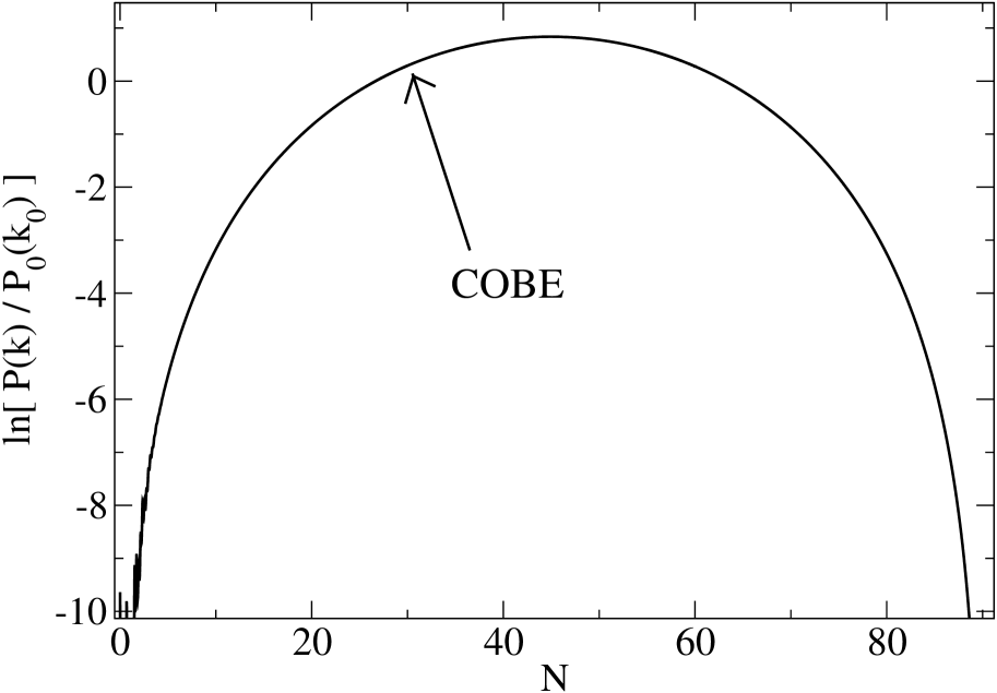
Figure 14: $\ln[P(k)/P_{0}(k_{0})]$ versus number of $e$-foldings since the beginning of inflation, where $\sqrt{P_{0}(k_{0})}=2\times 10^{-5}$ is the COBE normalization.

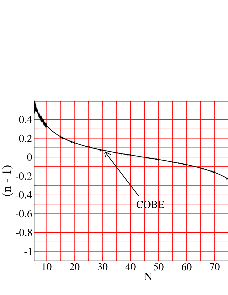
Figure 15: Scalar perturbation index as a function of $N$, related to wave number through $N\approx\ln k/H$.

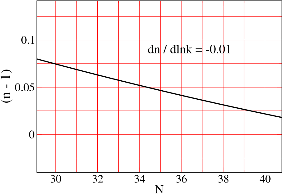
Figure 16: Closeup of the physically interesting region in figure XX, with $N\sim 30-39$ corresponding to wave numbers $k\sim 10^{-4}-1$ Mpc^-1.

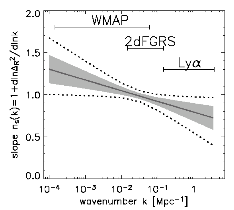
Figure 17: WMAP, LSS and Lyman $\alpha$ constraints on the spectral index from 68% (shaded area) and 95% (dashed lines) confidence level, from ref. [48].

The shape of the spectrum of scalar perturbations is shown in Fig. 15. It can be characterized by the spectral index $n_{s}$, defined as

$$n_{s}=1+{d\ln P(k)\over d\ln k}\,,$$ (40)

which for our typical solutions is the slope of Fig. 15. This is plotted explicitly in Figs. 15 and 17. Because it is difficult to obtain a large amount of inflation, the inflationary roll is not extremely slow, and the departure from a scale-free spectrum $(n_{s}=1)$ tends to be large. In the example shown, the spectrum is blue in the region relevant for the CMB and large scale structure formation (shown in Fig. 17), with $n_{s}\sim 1.03-1.08$.

This prediction from brane-antibrane inflation can be compared to observational constraints from the Wilkinson Microwave Anisotropy Probe (WMAP), the 2 degree Field Galaxy Redshift Survey (2dFGRS), and Lyman $\alpha$ forest data, which have been analyzed in ref. [48]. Fig. 17, borrowed from fig. 2 of [48], shows that our spectrum is well within the current limits. In comparing the prediction with the constraints, one should identify $N=30$ with $k=10^{-4}$ Mpc^-1, and $N=39$ with $k=1$ Mpc^-1. Present data are still consistent with a flat spectrum $n_{s}=1$ with no running, but there is a suggestion of large negative running, $dn/d\ln k\sim-0.04$, with large error bars. This hint is reiterated by a recent analysis combining WMAP data with that of Sloan Digital Sky Survey (SDSS), which obtained $dn/d\ln k=-0.07\pm 0.04$ [49]. The probability distribution function is reproduced in Fig. 19. If the trend toward negative running is confirmed in future CMB observations at a lower level than the present central value, it could be a signal in favor of the brane-antibrane model, which has $dn/d\ln k=-0.01$ in the region of interest in the example shown. We also plot $dn/d\ln k$ over the entire inflationary history in Fig. 19. This shows that larger values of $|dn/d\ln k|$ are indeed correlated with larger deviations of $n$ from unity, as one would expect from the theoretical slow-roll expressions for these quantities.

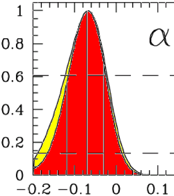
Figure 18: Probability distribution function for running of spectral index, $\alpha\equiv dn/d\ln k$, from combining WMAP and SDSS data [49].

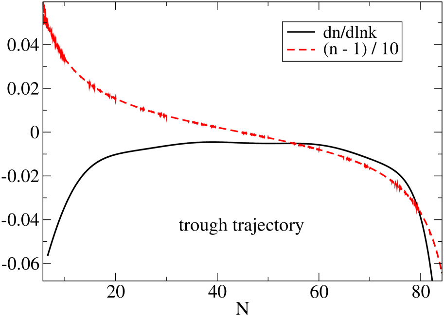
Figure 19: $dn/d\ln k$ (solid line) and $(n_{s}-1)/10$ (dashed line) versus $N$ for the inflaton trajectories in the trough.

More generally, Fig. 19 tells us how large a departure from a pure Harrison-Zeldovich ($n_{s}=1$) spectrum can be accommodated in the brane inflation model. To obtain larger deviations, the total duration of inflation can easily be shortened by relaxing the fine tuning of parameters. The visible region of the spectrum can thus be moved to lower values of $N$, leading to deviations as large as $n_{s}-1=0.5$, $|dn/d\ln k|=-0.06.$ Although Fig. 19 corresponds to the trough trajectories of Fig. 7, where the inflaton is identified with $\psi$, we have found that the central $\sigma$-like trajectory of fig. 11 produces a remarkably similar result for both $n_{s}$ and $dn/d\ln k$. On the other hand, interesting variations on this result can be found for the trajectories neighboring this central one, as shown in Figs. 21-21. The former is less favored by the data, since it has $dn/d\ln k>0$, but the latter is more consistent, and provides an example of obtaining distinctive features in the power spectrum, which could be revealed in future observations.

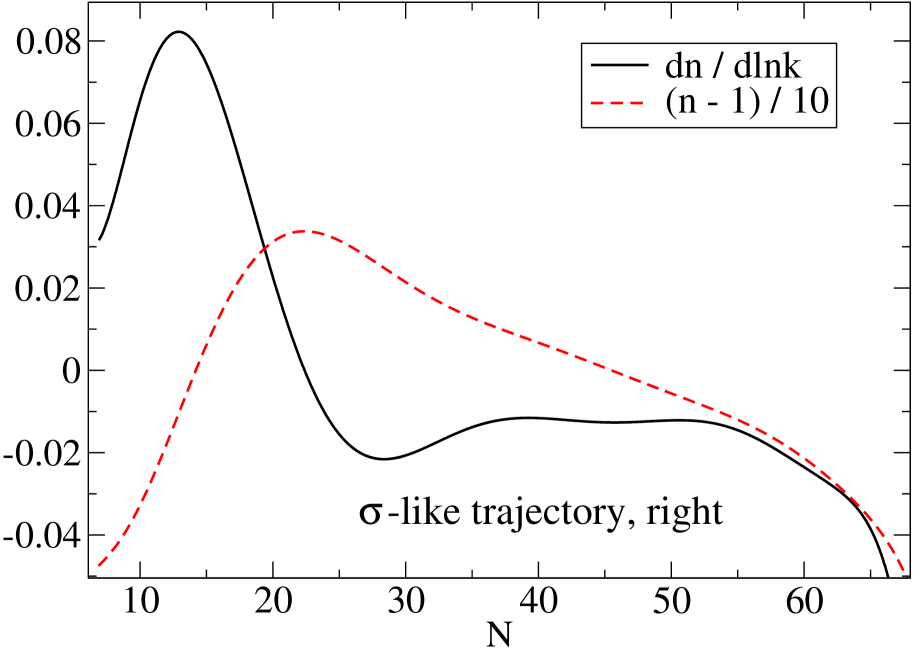
Figure 20: $dn/d\ln k$ (solid line) and $(n_{s}-1)/10$ (dashed line) versus $N$ for the $\sigma$-like trajectory starting on the right-hand-side of Fig. 11.

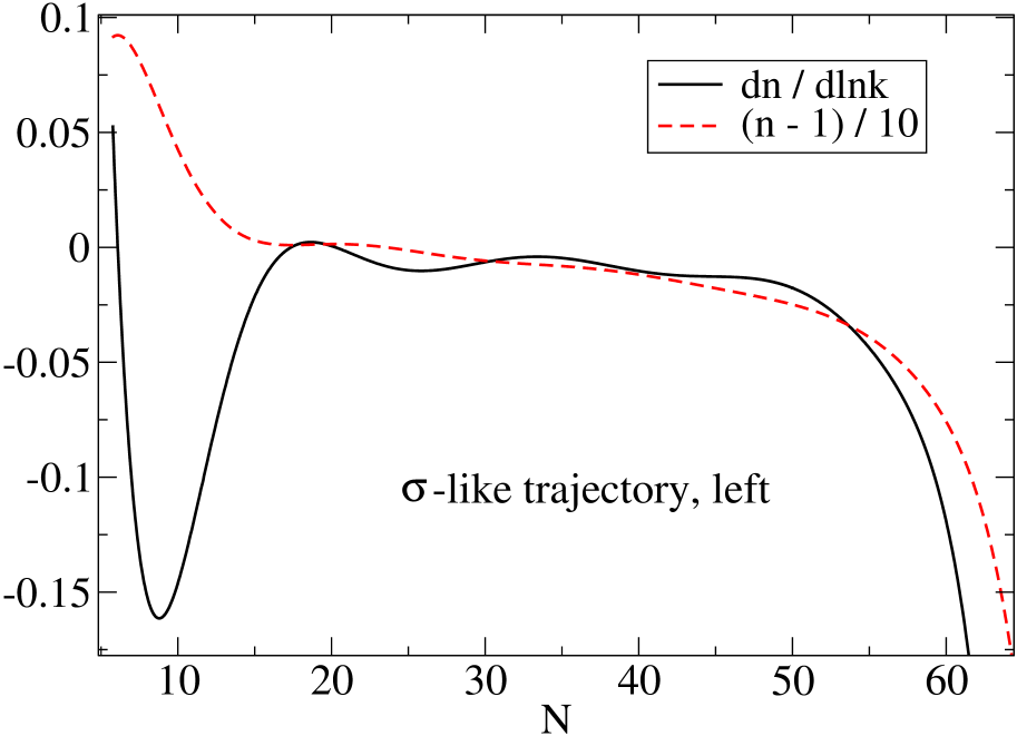
Figure 21: Same as previous figure, but for trajectory starting on the left-hand-side of Fig. 11.

Isocurvature Perturbations: In addition to the adiabatic (curvature) perturbations considered above, the presence of several fields makes it possible to generate entropy (isocurvature) perturbations–fluctuations in the light fields which are orthogonal to the inflaton trajectories. Isocurvature perturbations alter the shape of the acoustic peaks of the CMB fluctuation power spectrum, but only if the different light fields decay after inflation into particles with different equations of state (such as if $\psi$ decayed into cold dark matter and $\sigma$ decayed into radiation). At present there is no evidence for such perturbations, but only observational bounds on the level at which they can contribute to the temperature anisotropy [50]. Here we will not make a detailed analysis of their potential presence in brane-antibrane inflation; rather we just point out that some of our inflaton trajectories fulfill one of the necessary criteria for isocurvature modes to possibly be observable, namely there must be some curvature in field space of the inflaton trajectory [51]. In other words, the linear combination of fields which constitutes the inflaton must be time dependent. This possibility is demonstrated in Figs. 13-13, where significant twisting of the trajectories is evident. A more thorough investigation would be warranted if evidence for contamination by isocurvature modes is found in the data.

5 Comments and Conclusions

Our purpose in this paper is to see whether inflation can arise in the effective theory which captures the essential features of the low-energy limit of realistic string vacua in which the moduli are fixed at the string scale, as in refs. [19, 11, 15]. Several interesting features emerge from this investigation.

5.1 ‘Realistic’ Inflation

Our two main results are these:

1. Explicit Inflationary Solutions: We are able to explicitly identify inflationary trajectories within the 4D effective theory with fixed moduli. In so doing we allow all of the remaining moduli to roll. We find that inflation appears to be possible in these models even after moduli stabilization, representing definite progress over early work [1]-[6] for which moduli fixing was not addressed. As is usually the case for inflationary field theories, we find that obtaining a long period of inflation is not generic in the sense that it requires tuning of couplings and, to a lesser extent, initial conditions in field space.

In particular, we find that the relevant parameters must be adjusted to 1 part in 1000 in order to obtain 60 $e$-foldings of inflation. Once these parameters are so chosen, inflation occurs for a relatively wide range of initial field values (if the various fields all start from rest). The effective 4D theories have both $F$-term, $D$-term and supersymmetry-breaking contributions to their scalar potentials, and we find that all of these terms play an important role during inflationary evolution.

The inflationary solutions we find could well provide a good description of the observed CMB temperature fluctuations. Because it is difficult to obtain a slow roll, the predicted density fluctuations are typically not deep within the scale invariant regime. It is quite possible to obtain a scalar index observably different from unity (on the blue side for the examples considered), and for which $dn_{s}/d\ln k$ is different from zero. Because the inflationary roll is not very slow, observable tensor perturbations may also be produced.

2. The Standard Model and Reheating: We provide the first example of brane-antibrane inflation for which it is possible to identify the Standard Model degrees of freedom in the post-inflationary world. This opens up the exciting possibility of exploring all of the issues associated with reheating in the post-inflationary universe.

In the models studied in the greatest detail, the Standard Model lives on an antibrane at the tip of the throat, since this is the choice we made when using a $U(1)$ gauge coupling which is independent of $T$. (Presumably we are not living on the antibrane which is annihilated when the mobile brane reaches the end of the throat.) Since the tip of the throat can be highly warped, our possible presence there raises several interesting possibilities. It could be that the warping along the throat plays a role in the hierarchy problem, along the lines proposed by Randall and Sundrum. (Of course, this possibility conflicts with obtaining sufficiently large perturbations in the CMB within the large $r$ approximation within the inflationary solutions found here, because these latter two conditions led us to conclude the total warping should be small.) It is clearly an open question to obtain a string model with a realistic chiral spectrum of quarks and leptons, with all moduli fixed in such a way that a hierarchy is naturally obtained after supersymmetry breaking and the scales are also the ones preferred by the inflation/density perturbation requirements. It would be well worth further exploring the model-building possibilities along these lines. On the other hand if the scale preferred by inflation does not match the one needed for a phenomenologically realistic model after supersymmetry breaking, a two-throat scenario may be considered in which inflation happens in one throat with probably not much warping, whereas the standard model lies on a different throat with enough warping to generate the hierarchy in the scales.

If strong warping could be produced at the throat’s tip in a way consistent with inflation, this might open up other attractive possibilities for cosmology. In particular, since the warping tends to reduce the effective tension of the D3 brane as it falls down the throat, the energy density released by the final brane-antibrane annihilation is likely to be set by a lower scale (like the weak scale) rather than the much higher string or Planck scales. This may be too little to pay the cost of exciting the comparatively high string-scale masses of states in the bulk or on branes situated further away from the throat. If so, then the warping of the throat may act to improve the efficiency with which inflationary energy gets converted into reheating standard model degrees of freedom as opposed to populating phenomenologically problematic bulk states. A full consideration of this process would be very interesting to pursue but it lies beyond the scope of the present article. A particularly interesting possibility in this context is the generation of topological defects such as cosmic strings after inflation, such has been discussed in [55, 56]. In particular the structure of the models presented here seems to fit in the class of scenarios discussed by Copeland, Myers and Polchinski [56], for which no stable cosmic strings survive.

5.2 String Theory and Double Inflation

Although we are able to obtain 60 $e$-foldings of inflation for some initial conditions, since this is not the generic situation it is worth standing back and asking whether string theory is trying to tell us something when it makes inflation not so easy to achieve.

On reflection there are two things that emerge from the search for inflation in string theory as being rather generic.

$\bullet$ It is difficult to obtain 60 $e$-foldings of inflation at energies near the string scale, largely because the theory does not have many small dimensionless numbers with which to work. (In fact the tunings we required were special values of not particularly small couplings, rather than unnaturally small values.) Although there are many scalar fields which are free to roll at very high energies, the periods of potential-energy domination which result are normally not long enough to produce a full 60 $e$-foldings. 10 to 20 $e$-foldings are much easier to obtain however, and perhaps this suggests that string theory prefers to only give a small number of $e$-foldings during the inflationary phase which produces the observed temperature fluctuations in the microwave background.

$\bullet$ String vacua are normally rife with moduli, which generically acquire masses only after supersymmetry breaks. Thus, there are likely to be numerous scalar fields whose masses are comparatively small since they are close to the weak scale, $M_{w}$. Such scalars generically cause problems for cosmology since they give rise to a host of cosmological moduli problems [54] during the Hot Big Bang. Many of these problems would not arise if the universe were to undergo a period of late-time inflation [57].

Perhaps these two points can lead to a more generic picture of inflation within string theory. In this picture CMB temperature fluctuations are produced by an inflationary period involving energy densities near the string scale, but lasting for only 10 or more $e$-foldings. The remainder of the 60 $e$-foldings required to explain the Big Bang’s flatness and homogeneity problems arise during a second period of inflation which is associated with the rolling of the many string moduli whose masses are of order the weak scale. For instance the slowness of this later rolling might be due to a mechanism along the lines proposed in ref. [58].

If this picture is borne out as a bona fide string prediction, then it implies several observational consequences.

• First, the observed CMB temperature fluctuations should not be deep into the slow-roll regime because $N_{e}\ll 60$, and so should not be extremely close to the scale invariant predictions. In particular we might expect to find slow-roll parameters $\epsilon$ and $\eta$ which are on the larger side of their allowed ranges, perhaps being of order $1/N_{e}\sim 0.1$. Besides more easily accommodating phenomena like kinks in the inflationary spectrum and a running spectral index, this would imply that tensor perturbations might be detected in the near future.

• Second, it predicts a period of late inflation, and so requires any explanation of phenomena like baryon-number generation to necessarily take place at comparatively low energies like the electroweak scale.

We believe this kind of picture may well represent a more natural reconciliation between the requirements of inflation and the properties of known string vacua. If so, it would provide a natural explanation for effects like a running spectral index, which may have been observed in the primordial fluctuation spectrum. We believe more detailed studies of cosmologies of this sort are warranted given the motivation this kind of picture may receive both from string theory and the current data.

In summary, we have seen how inflation can arise in an effective theory which captures the essential features of the low-energy limit of realistic string vacua with moduli fixed at the string scale. We believe that we are just seeing the beginnings of the exploration of inflation in string vacua, and that with the recent advent of string vacua for which many moduli are fixed at the string scale [19], much remains to be done towards the goal of a systematic investigation of the properties of string-based inflation.

6 Acknowledgements

We would like to thank J. Blanco-Pilado, C. Escoda, H. Firouzjahi, M. Gómez-Reino, N. Jones, S. Kachru, R. Kallosh, A. Linde, J. Maldacena, S. Trivedi, H. Tye and A. Uranga for helpful discussions on these and related subjects. We thank the organizers of the KITP workshop on string cosmology for providing the perfect environment to start this work. C.B. is funded by NSERC (Canada), FCAR (Québec) and McGill University. F.Q. is partially funded by PPARC and the Royal Society Wolfson award.

References

- [1] C. P. Burgess, M. Majumdar, D. Nolte, F. Quevedo, G. Rajesh and R. J. Zhang, “The inflationary brane-antibrane universe,” JHEP 0107 (2001) 047 [hep-th/0105204].
- [2] G. R. Dvali, Q. Shafi and S. Solganik, “D-brane inflation,” [hep-th/0105203].
- [3] C. P. Burgess, P. Martineau, F. Quevedo, G. Rajesh and R. J. Zhang, “Brane antibrane inflation in orbifold and orientifold models,” JHEP 0203 (2002) 052 [hep-th/0111025].
- [4] S. H. Alexander, “Inflation from D - anti-D brane annihilation,” Phys. Rev. D 65 (2002) 023507 [hep-th/0105032].
- [5] C. Herdeiro, S. Hirano and R. Kallosh, “String theory and hybrid inflation / acceleration,” JHEP 0112 (2001) 027 [arXiv:hep-th/0110271]; K. Dasgupta, C. Herdeiro, S. Hirano and R. Kallosh, “D3/D7 inflationary model and M-theory,” Phys. Rev. D 65 (2002) 126002 [arXiv:hep-th/0203019]; J. Garcia-Bellido, R. Rabadan and F. Zamora, “Inflationary scenarios from branes at angles,” JHEP 0201 (2002) 036 [hep-th/0112147]; N. Jones, H. Stoica and S. H. Tye, “Brane interaction as the origin of inflation,” JHEP 0207 (2002) 051 [hep-th/0203163]; M. Gomez-Reino and I. Zavala, “Recombination of intersecting D-branes and cosmological inflation,” JHEP 0209 (2002) 020 [hep-th/0207278].
- [6] G. R. Dvali and S. H. H. Tye, “Brane inflation,” Phys. Lett. B 450 (1999) 72 [hep-ph/9812483].
- [7] A. D. Linde, “Hybrid inflation,” Phys. Rev. D 49 (1994) 748 [astro-ph/9307002].
- [8] For a recent discussion including many references, see: A. Fotopoulos and A. A. Tseytlin, “On open superstring partition function in inhomogeneous rolling tachyon background,” hep-th/0310253; A. Sen, “Remarks on tachyon driven cosmology,” arXiv:hep-th/0312153.
- [9] S. Kachru, R. Kallosh, A. Linde, J. Maldacena, L. McAllister and S. P. Trivedi, “Towards inflation in string theory,” hep-th/0308055.
- [10] S. Buchan, B. Shlaer, H. Stoica and S. H. H. Tye, “Inter-brane interactions in compact spaces and brane inflation,” hep-th/0311207.
- [11] S. Kachru, R. Kallosh, A. Linde and S. P. Trivedi, “de Sitter Vacua in String Theory,” [hep-th/0301240].
- [12] See for instance: E. J. Copeland, A. R. Liddle, D. H. Lyth, E. D. Stewart and D. Wands, “False vacuum inflation with Einstein gravity,” Phys. Rev. D 49 (1994) 6410 [astro-ph/9401011].
- [13] P. Binetruy and G. R. Dvali, “D-term inflation,” Phys. Lett. B 388 (1996) 241 [hep-ph/9606342].
- [14] T. Kobayashi and O. Seto, “Dilaton and moduli fields in D-term inflation,” Phys. Rev. D 69, 023510 (2004) [arXiv:hep-ph/0307332]; T. Higaki, T. Kobayashi and O. Seto, “D-term inflation and nonperturbative Kaehler potential of dilaton,” arXiv:hep-ph/0402200.
- [15] J. F. G. Cascales, M. P. Garcia del Moral, F. Quevedo and A. M. Uranga, “Realistic D-brane models on warped throats: Fluxes, hierarchies and moduli stabilization,” hep-th/0312051.
- [16] L. Randall and R. Sundrum, “A large mass hierarchy from a small extra dimension,” Phys. Rev. Lett. 83 (1999) 3370 [hep-ph/9905221].
- [17] H. Verlinde, “Holography and compactification,” Nucl. Phys. B 580 (2000) 264 [hep-th/9906182].
- [18] S. Sethi, C. Vafa and E. Witten, “Constraints on low-dimensional string compactifications,” Nucl. Phys. B 480 (1996) 213 [arXiv:hep-th/9606122]; K. Dasgupta, G. Rajesh and S. Sethi, “M theory, orientifolds and G-flux,” JHEP 9908 (1999) 023 [arXiv:hep-th/9908088].
- [19] S. B. Giddings, S. Kachru and J. Polchinski, “Hierarchies from fluxes in string compactifications,” Phys. Rev. D66, 106006 (2002).
- [20] S. Gukov, C. Vafa and E. Witten, “CFTs from Calabi-Yau Fourfolds,” Nucl. Phys. B584, 69 (2000).
- [21] E. Witten, “Dimensional Reduction Of Superstring Models,” Phys. Lett. B 155 (1985) 151; C. P. Burgess, A. Font and F. Quevedo, “Low-Energy Effective Action For The Superstring,” Nucl. Phys. B 272 (1986) 661.
- [22] E. Cremmer, S. Ferrara, C. Kounnas and D.V. Nanonpoulos, “Naturally vanishing cosmological constant in supergravity,” Phys. Lett. B133, 61 (1983); J. Ellis, A.B. Lahanas, D.V. Nanopoulos and K. Tamvakis, “No-scale Supersymmetric Standard Model,” Phys. Lett. B134, 429 (1984).
- [23] J. P. Derendinger, L. E. Ibanez and H. P. Nilles, “On The Low-Energy D = 4, N=1 Supergravity Theory Extracted From The D = 10, N=1 Superstring,” Phys. Lett. B 155 (1985) 65; M. Dine, R. Rohm, N. Seiberg and E. Witten, “Gluino Condensation In Superstring Models,” Phys. Lett. B 156 (1985) 55.
- [24] C.P. Burgess, J.-P. Derendinger, F. Quevedo and M. Quirós, “Gaugino Condensates and Chiral-Linear Duality: An Effective-Lagrangian Analysis”, Phys. Lett. B 348 (1995) 428–442; “On Gaugino Condensation with Field-Dependent Gauge Couplings”, Ann. Phys. 250 (1996) 193-233.
- [25] C. Escoda, M. Gomez-Reino and F. Quevedo, “Saltatory de Sitter string vacua,”JHEP 0311 (2003) 065, hep-th/0307160.
- [26] C. P. Burgess, R. Kallosh and F. Quevedo, “de Sitter string vacua from supersymmetric D-terms,” JHEP 0310 (2003) 056 [hep-th/0309187].
- [27] A. Saltman and E. Silverstein, “The Scaling of the No Scale Potential and de Sitter Model Building,” [hep-th/0402135].
- [28] R. Brustein and S. P. de Alwis, “Moduli potentials in string compactifications with fluxes: Mapping the discretuum,” arXiv:hep-th/0402088.
- [29] J. Hughes and J. Polchinski, “Partially Broken Global Supersymmetry And The Superstring,” Nucl. Phys. B 278 (1986) 147. R. Altendorfer and J. Bagger, “Dual supersymmetry algebras from partial supersymmetry breaking,” Phys. Lett. B 460 (1999) 127 [hep-th/9904213]; C. P. Burgess, E. Filotas, M. Klein and F. Quevedo, “Low-energy brane-world effective actions and partial supersymmetry breaking,” JHEP 0310 (2003) 041 [hep-th/0209190].
- [30] O. De Wolfe and S.B. Giddings, “Scales and Hierarchies in Warped Compactifications and Brane Worlds,” Phys. Rev. D67 (2003) 066008 [hep-th/0208123].
- [31] C.P. Burgess and C.A. Lütken, Phys. Lett. B153 (1985) 137.
- [32] J. P. Hsu, R. Kallosh and S. Prokushkin, “On brane inflation with volume stabilization,” JCAP 0312 (2003) 009 [hep-th/0311077];
- [33] R. Kallosh and S. Prokushkin, “SuperCosmology,” arXiv:hep-th/0403060.
- [34] H. Firouzjahi and S. H. H. Tye, “Closer towards inflation in string theory,” hep-th/0312020.
- [35] A. Buchel and R. Roiban, “Inflation in warped geometries,” arXiv:hep-th/0311154; E. Halyo, “D-brane inflation on conifolds,” arXiv:hep-th/0402155.
- [36] L. Pilo, A. Riotto and A. Zaffaroni, “Old inflation in string theory,” hep-th/0401004.
- [37] G. Aldazabal, L. E. Ibanez, F. Quevedo and A. M. Uranga, “D-branes at singularities: A bottom-up approach to the string embedding of the standard model,” JHEP 0008 (2000) 002 [hep-th/0005067].
- [38] M. Dine, N. Seiberg and E. Witten, “Fayet-Iliopoulos Terms In String Theory,” Nucl. Phys. B 289 (1987) 589.
- [39] P. Binetruy, G. Dvali, R. Kallosh and A. Van Proeyen, [hep-th/0402046].
- [40] P. Fayet and J. Iliopoulos, “Spontaneously Broken Supergauge Symmetries And Goldstone Spinors,” Phys. Lett. B 51 (1974) 461.
- [41] J. M. Cornwall, D. N. Levin and G. Tiktopoulos, “Derivation Of Gauge Invariance From High-Energy Unitarity Bounds On The S - Matrix,” Phys. Rev. D 10 (1974) 1145 [Erratum-ibid. D 11 (1975) 972]; C. P. Burgess and D. London, “Uses and abuses of effective Lagrangians,” Phys. Rev. D 48 (1993) 4337 [hep-ph/9203216].
- [42] P. G. Camara, L. E. Ibanez and A. M. Uranga, “Flux-induced SUSY-breaking soft terms,” [hep-th/0311241].
- [43] See for instance: S. Groot Nibbelink and B. J. W. van Tent, “Density perturbations arising from multiple field slow-roll inflation,” [hep-ph/0011325]; C. P. Burgess, P. Grenier and D. Hoover, “Quintessentially flat scalar potentials,” [hep-ph/0308252].
- [44] J. M. Cline, H. Firouzjahi and P. Martineau, “Reheating from tachyon condensation,” JHEP 0211, 041 (2002) [hep-th/0207156]; J. M. Cline and H. Firouzjahi, “Real-time D-brane condensation,” Phys. Lett. B 564, 255 (2003) [arXiv:hep-th/0301101]; N. Barnaby and J. M. Cline, in preparation
- [45] D. H. Lyth and A. Riotto, “Particle physics models of inflation and the cosmological density perturbation,” Phys. Rept. 314, 1 (1999) [hep-ph/9807278].
- [46] A. Cooray, “After MAP: Next generation CMB,” [astro-ph/0211347].
- [47] L. Knox and Y. S. Song, “A limit on the detectability of the energy scale of inflation,” Phys. Rev. Lett. 89, 011303 (2002) [astro-ph/0202286]; M. Kesden, A. Cooray and M. Kamionkowski, “Separation of gravitational-wave and cosmic-shear contributions to cosmic microwave background polarization,” Phys. Rev. Lett. 89, 011304 (2002) [astro-ph/0202434]. W. H. Kinney, “The energy scale of inflation: Is the hunt for the primordial B-mode a waste of time?,” [astro-ph/0307005].
- [48] H. V. Peiris et al., “First year Wilkinson Microwave Anisotropy Probe (WMAP) observations: Implications for inflation,” Astrophys. J. Suppl. 148, 213 (2003) [astro-ph/0302225].
- [49] M. Tegmark et al. [SDSS Collaboration], “Cosmological parameters from SDSS and WMAP,” [astro-ph/0310723].
- [50] P. Crotty, J. Garcia-Bellido, J. Lesgourgues and A. Riazuelo, “Bounds on isocurvature perturbations from CMB and LSS data,” Phys. Rev. Lett. 91, 171301 (2003) [astro-ph/0306286]; M. Bucher, J. Dunkley, P. G. Ferreira, K. Moodley and C. Skordis, “The initial conditions of the universe: how much isocurvature is allowed?,” arXiv:astro-ph/0401417.
- [51] C. Gordon, D. Wands, B. A. Bassett and R. Maartens, “Adiabatic and entropy perturbations from inflation,” Phys. Rev. D 63, 023506 (2001) [astro-ph/0009131].
- [52] S. Kachru, J. Pearson and H. Verlinde, “Brane/Flux Annihilation and the String Dual of a Non-Supersymmetric Field Theory,” JHEP 0206, 021 (2002) [hep-th/0112197].
- [53] N. V. Krasnikov, “On Supersymmetry Breaking In Superstring Theories,” Phys. Lett. B 193 (1987) 37.
- [54] G. D. Coughlan, W. Fischler, E. W. Kolb, S. Raby and G. G. Ross, “Cosmological Problems For The Polonyi Potential,” Phys. Lett. B 131 (1983) 59; B. de Carlos, J. A. Casas, F. Quevedo and E. Roulet, “Model independent properties and cosmological implications of the dilaton and moduli sectors of 4-d strings,” Phys. Lett. B 318 (1993) 447 [hep-ph/9308325]; T. Banks, D. B. Kaplan and A. E. Nelson, “Cosmological implications of dynamical supersymmetry breaking,” Phys. Rev. D 49 (1994) 779 [hep-ph/9308292].
- [55] N. T. Jones, H. Stoica and S. H. H. Tye, “The production, spectrum and evolution of cosmic strings in brane inflation,” Phys. Lett. B 563 (2003) 6 [hep-th/0303269]; L. Pogosian, S. H. H. Tye, I. Wasserman and M. Wyman, “Observational constraints on cosmic string production during brane inflation,” Phys. Rev. D 68 (2003) 023506 [hep-th/0304188]; M. Majumdar and A. Christine-Davis, “Cosmological creation of D-branes and anti-D-branes,” JHEP 0203 (2002) 056 [arXiv:hep-th/0202148]; G. Dvali and A. Vilenkin, “Formation and evolution of cosmic D-strings,” hep-th/0312007; G. Dvali, R. Kallosh and A. Van Proeyen, “D-term strings,” JHEP 0401 (2004) 035 [hep-th/0312005].
- [56] E. J. Copeland, R. C. Myers and J. Polchinski, “Cosmic F- and D-strings,” hep-th/0312067.
- [57] D. H. Lyth and E. D. Stewart, “Thermal inflation and the moduli problem,” Phys. Rev. D 53, 1784 (1996) [arXiv:hep-ph/9510204].
- [58] G. Dvali and S. Kachru, “New old inflation,” hep-th/0309095.