Field theory on a Non–commutative Plane: a Non–perturbative Study
⋆⋆\star⋆⋆\starSlightly modified PhD thesis, accepted at Humboldt–Universität zu Berlin in March 2003, defended
in June 2003.
Frank Hofheinz
Institut für Physik, Humboldt–Universität zu Berlin
Newtonstr. 15, D–12489 Berlin, Germany
E–mail: hofheinz@physik.hu-berlin.de
Abstract: The 2d gauge theory on the lattice is equivalent to the twisted Eguchi–Kawai model, which we simulated at ranging from 25 to 515. We observe a clear large scaling for the 1– and 2–point function of Wilson loops, as well as the 2–point function of Polyakov lines. The 2–point functions agree with a universal wave function renormalization. The large double scaling limit corresponds to the continuum limit of non–commutative gauge theory, so the observed large scaling demonstrates the non–perturbative renormalizability of this non–commutative field theory. The area law for the Wilson loops holds at small physical area as in commutative 2d planar gauge theory, but at large areas we find an oscillating behavior instead. In that regime the phase of the Wilson loop grows linearly with the area. This agrees with the Aharonov–Bohm effect in the presence of a constant magnetic field, identified with the inverse non–commutativity parameter.
Next we investigate the 3d model with two non–commutative coordinates and explore its phase diagram. Our results agree with a conjecture by Gubser and Sondhi in , who predicted that the ordered regime splits into a uniform phase and a phase dominated by stripe patterns. We further present results for the correlators and the dispersion relation. In non–commutative field theory the Lorentz invariance is explicitly broken, which leads to a deformation of the dispersion relation. In one loop perturbation theory this deformation involves an additional infrared divergent term. Our data agree with this perturbative result.
We also confirm the recent observation by Ambjørn and Catterall that
stripes occur even in , although they imply the spontaneous
breaking of the translation symmetry.
Keywords: Non–commutative Geometry, Matrix Models, Lattice Gauge Theory, Field Theory in lower Dimensions
1 Introduction
The ideas of non–commutative space–time and field theories defined on such a structure started already in the year 1947. At this time the concept of renormalization was not yet well established and therefore ultraviolet divergences in quantum field theory still caused serious problems. To solve these problems or at least weaken them Snyder introduced the quantized space–time [1] (see also [2]).
The plan was to define quantum field theories on a space–time which is smeared out at very small length scales. This means that in addition to Heisenberg’s uncertainty relation between coordinates and momenta there is a uncertainty between different coordinates.
As in the quantization of the classical phase space, space–time can be quantized by replacing the usual coordinates by Hermitian operators , obeying the commutator relation
| (1.1) |
The non–commutativity tensor is a real–valued antisymmetric matrix and is the space–time dimension. Since the coordinate operators do not commute they cannot be diagonalized simultaneously and therefore induce the uncertainty relation
| (1.2) |
This uncertainty implies a quantum structure of space–time and due to the lack of points in space–time it then represents an effective ultraviolet cut–off.
Much later, in 1996, it was shown by Filk [3] that in
field theory on a non–commutative plane the divergences of
commutative field theory still occur. In addition to those divergences
the authors of Refs. [4, 5] found in 1999
that
there is a mixing of ultraviolet and infrared divergences.
The concept of quantized space–time has not been followed further in the early days of quantum field theory, since the renormalization technique became more and more successful. It came up again first in the 80’s, when Connes formulated the mathematically rigorous [6] framework of non–commutative geometry. In physical theories a non–commutative space–time first appeared in string theory, namely in the quantization of open strings [7]. In an constant magnetic background field the boundary conditions change and the zero momentum modes of the string do not commute anymore. Instead they obey a commutation relation of the type (1.1), where is proportional to the inverse background field.
The zero momentum modes of an open string can be interpreted as the
end points of the string, which are confined to a submanifold, i.e. a D–brane. The commutator (1.1) implies a
non–commutative geometry on the branes. Hence a quantized space–time
appears naturally in string
theory [8].
Another field of interest, where the non–commutativity of space–time
could play an important role, is quantum gravity. It is an old believe
that for a quantized theory of gravitation space–time has to change
its nature on very small length scales. The synthesis of the
principles of quantum mechanics and of classical general relativity
leads to a space–time uncertainty
[9, 10], which implies that any
theory of quantum gravity will not be local in the conventional sense
[11].
Such effects could be modeled by a non–commutative space–time.
Also in condensed matter physics the concept of non–commutative space–time is applied. The theory of electrons in a magnetic field projected to the lowest Landau level can be naturally described by a non–commutative field theory [12, 13, 14, 15, 16], where is again proportional to the inverse magnetic field. These ideas are relevant for the quantum Hall effect. For the integer quantum Hall effect, a non–commutative treatment serves as an alternative description to standard condensed matter techniques. This is already remarkable, since it is the first application of non–commutativity geometry that provides phenomenological results. However, with these methods only the known results are reproduced; it does not provide new insight in the nature of the integer quantum Hall effect.
This may be different in the case of the fractional quantum Hall
effect. That effect is not well understood from the theoretical point
of view. Here a non–commutative field theory is considered by many
researchers as the most promising candidate for a description.
One may also try to study the non–commutative analog of pure
Yang–Mills theories or of QED and QCD. Such theories can be
considered as an extended standard model and a study of them could
allow for an experimental verification or falsification. Hence results
from these extended theories may provide sensible tests of a quantized
space–time.
The above described applications of non–commutative field theory suffer from the ultraviolet/infrared (UV/IR) mixing. This effect causes still severe problems in a perturbative treatment. Our goal is to study non–commutative field theories on a completely non–perturbative level.
This work represents the first non–perturbative study of non–commutative field theories. As usual when entering a new topic we studied toy models, which share important properties of the full theory. In this work we studied field theory in lower dimensions and we focused on basic properties of these theories. The results presented here are published in Refs. [17, 18, 19].
In a two dimensional gauge theory we address the problem of
renormalizability.
It is an interesting question whether this
model can be renormalized non–perturbatively.
In the three dimensional theory we studied the effects
of UV/IR mixing. Our main interest was here the phase diagram of this
theory and the question if there is a phase with spontaneously broken
translation invariance, as it had been conjectured from analytic
results. In addition we studied the dispersion relation in
this theory, for which perturbation theory predicts a deformation due
to the non–commutativity.
This work is organized as follows: in Chapter 2 we give an introduction to non–commutative field theory. We concentrate here on the main differences compared to commutative field theory. In a first Section we set up the non–commutative geometry on which we define a scalar field theory and a pure gauge theory (Sections 2.2 and 2.3, respectively). These are the theories studied in this work. In Section 2.4 we briefly comment on the extension to the non–commutative standard model. In addition to the motivation already given in the introduction we want to motivate the study of non–commutative space–time from this point of view.
Chapter 3 is dedicated to the lattice regularization. As we already mentioned in this introduction the non–commutativity of space–time does not cure the ultraviolet divergences, and therefore one still has to regularize the theory. To this end we will introduce a momentum cut–off via discretization of space–time.
In Chapter 4 and 5 we present the two models we
investigated; a two dimensional non–commutative pure gauge theory and
a three dimensional scalar field theory. The explicit construction of
the lattice actions as well as the Monte Carlo results of our studies
are presented in these Chapters. In Chapter 6 we show results
on a two dimensional scalar theory, and in Chapter 7 we
summarize our results and give an outlook. For the sake of continuity
the details of the simulations are banned
to Appendix A.
Note that throughout this work we always work in Euclidean space–time. We should mention here that in contrast to the commutative case, it is an open question if the Euclidean version of non–commutative field theory can be interpreted in the Minkowski world, since there is no equivalent of the Osterwalder–Schrader theorem [20]. However, in non–commutative field theory with a commuting time coordinate it is generally believed that this interpretation exists. For a discussion of Wick rotation and the related question of unitarity, see e.g. Refs. [21, 22, 23].
Chapter 2 Non–commutative field theory
In this Chapter we give an introduction to the concept of non–commutative space–time and field theories defined on it. We will work out the main differences to their commutative counterparts and discuss the additional problems that arise in such theories. For a general discussion of non–commutative space–time see for example Refs. [24, 11]. We follow here the discussion in Refs. [25, 26].
2.1 Non–commutative flat space–time
In this Section we discuss those features of non–commutative geometry, which are needed to define field theories on such a geometry. We will find two alternative formulations, in terms of Weyl operators and in terms of functions with a deformed multiplication.
2.1.1 Weyl operators
Let us start with the commutative algebra of complex valued functions on dimensional Euclidean space–time . An element of this algebra corresponds to a configuration of a scalar field, with pointwise addition and multiplication. We consider here functions of sufficiently rapid decrease at infinity, so that any function may be described by its Fourier transform
| (2.1) |
A non–commutative space–time can be defined by replacing the local coordinates by Hermitian operators satisfying
| (2.2) |
The non–commutativity tensor is antisymmetric with the dimension length squared and it can in general depend on space–time. Here we restrict ourselves to a constant non–commutativity tensor parametrized by the non–commutativity parameter
| (2.3) |
Here we assume the space–time dimension to be even. The generate a non–commutative and associative algebra of operators. Elements of this algebra, the Weyl operators , can be constructed by a formal Fourier transform involving the operators and the ordinary Fourier transform of
| (2.4) |
Combining equations (2.1) and (2.4) we find an explicit map between operators and fields
| (2.5) |
where is a Hermitian operator that can be understood as a mixed basis for operators of fields.
We may define a linear and anti–Hermitian derivative on the algebra of Weyl operators by the commutator relations
| (2.6) |
where is a real valued c–number. With this definition of the derivative one can show that
| (2.7) |
Together with equation (2.5) and integration by parts one obtains that the derivative of Weyl operators is equal to the Weyl operator of the usual derivative of the functions
| (2.8) |
Any global translation with can be obtained with the unitary operators
| (2.9) |
This follows directly from the commutator relation (2.7). This property implies that any trace , with Tr defined on the algebra of Weyl operators, is independent of . Together with equation (2.7) it follows that the trace Tr is unambiguously given by an integration over space–time
| (2.10) |
with the normalization .
In Ref. [26] it is shown that if is invertible (which implies that the dimension of space–time has to be even) the product of two operators at distinct points can be computed as follows
| (2.11) |
Together with the normalization of the trace the operators form an orthonormal set for ,
| (2.12) |
With this property of we can define the inverse map to (2.5)
| (2.13) |
This one–to–one correspondence can be thought of as an analog of the operator–state correspondence in quantum mechanics.
2.1.2 The star–product
Let us now consider the product of two Weyl operators corresponding to the two functions and . We want to transform this product into the coordinate space representation with the help of the inverse map (2.13),
| (2.14) |
To achieve this we rewrite the product in terms of the map (2.5)
| (2.15) |
where in the second line equation (2.11) was used. Multiplying both sides with from the right and taking the trace leads to
| (2.16) |
where we used the completeness relation (2.12). Using this product we obtain
| (2.17) |
i.e. the product of Weyl operators is equal to the Weyl operator of the star–products of functions in coordinate space. With the star–product we can rewrite the commutation relation between space–time operators (2.2) in terms space–time coordinates
| (2.18) |
The star–product is associative but non–commutative. For it reduces to the ordinary product of functions. It can be thought of as a deformation of the algebra of functions on to a non–commutative algebra, with the same elements and addition law, but with a different multiplication law given by (2.16). Note that the commutator of a function with the coordinates can be used to generate derivatives
| (2.19) |
Due to the cyclicity of the trace defined in equation (2.10) the integral
| (2.20) |
is invariant under cyclic permutations of the functions . In
particular the integral of the star–product of two
functions is identical to the integral of the ordinary product
of two functions
| (2.21) |
We have now two ways to encode non–commutative space–time:
-
•
we can use ordinary products in the non–commutative –algebra of Weyl operators,
-
•
or we may deform the ordinary product of the commutative –algebra of functions in to the non–commutative star–product.
2.1.3 The non–commutative torus
In this Subsection we briefly discuss the case when space–time is a –dimensional torus instead of . For a more detailed discussion, see [25, 26].
Let us consider functions on a periodic torus
| (2.22) |
is the unit vector in the direction and is the period matrix of the torus. Due to this periodicity the momenta in (2.1) are discretized according to
| (2.23) |
Using the discrete version of Fourier transform (2.1) we can define a mapping from fields to operators in the same way as we did in flat . The result is
| (2.24) |
where we introduced the dimensionless non-commutativity tensor
| (2.25) |
and the operators
| (2.26) |
With this mapping we find the one–to–one correspondence (2.5) and (2.13) also on the non–commutative torus. These definitions will reappear in Section 3.1, where we discuss the discrete torus.
2.2 Non–commutative scalar field theory
Having defined the algebra of functions of non–commutative space–time we are able to define a scalar field theory on this geometry. At this point we make a change of notation and introduce the short–hand notation for Weyl operators .
2.2.1 Non–commutative scalar action
We start our discussion with the action of an Euclidean commutative theory,
| (2.27) |
where is a real valued scalar field and is the dimension of space–time.
To transform an ordinary scalar field theory to a non–commutative field theory we can use one of the procedures described in the last Section. Either we may use the Weyl quantization via Hermitian operators , or we use the deformation of the product into the star–product (2.16).
The quantum field theory written in terms of Weyl operators , corresponding to a real scalar field on , reads
| (2.28) |
where the kinetic term is a direct consequence of equation (2.8) (it involves a sum over ). The measure is here the ordinary path integral measure for scalar fields .
This theory may be formulated in coordinate space by applying the map (2.13) to the action (2.28) and using equation (2.17),
| (2.29) |
the kinetic term and the mass term do not contain the star–product, because of the property (2.21) of the star–product. As a consequence the commutative and the non–commutative theory coincide for free fields. The difference arises due to the self–interaction term
| (2.30) |
with the interaction vertex in momentum space
| (2.31) |
This vertex contains a momentum dependent phase factor and it is therefore non–local.
2.2.2 UV/IR mixing
We discuss this important difference of non–commutative field theories compared to commutative theories at the example of one loop mass renormalization of the 4d theory, given by equation (2.29). To this end we consider the one particle irreducible two–point function
| (2.32) |
At lowest order the two–point function is given by . The one loop contribution splits topologically into two parts, one planar and one non–planar diagram
| (2.33) | |||||
| (2.34) |
In Refs. [3, 4] it is shown that the contribution of planar diagrams to non–commutative perturbation theory is proportional to the commutative case (to all orders). Therefore the planar divergences may be absorbed into the bare parameters, if and only if the corresponding commutative theory is renormalizable. This already disproves the expectation that non–commutative quantum field theory would not require renormalization.
In the case of the non–planar diagrams the situation is different. Rewriting the denominator in equation (2.34) in terms of a Schwinger parameter
| (2.35) |
and introducing a momentum cut–off by multiplying the resulting integrand in (2.34) with a Pauli–Villars regulator , leads in dimensions to [26]
| (2.36) |
where is the irregular modified Bessel function of order . In the leading divergences of equation (2.36) are given by
| (2.37) |
Here we introduced the effective cut–off given by
| (2.38) |
The two–point function remains finite in the limit , because it is effectively regulated by the non–commutative space–time. The complete one loop corrected propagator then reads
| (2.39) |
where we used
| (2.40) |
The UV limit () does not commute with the IR limit () or with the limit . At small momenta or small non–commutativity parameter the two–point function reads
| (2.41) |
Taking now the UV limit leads to the standard mass renormalization of the theory. Taking these limits vice versa, the effective cut–off is given by
| (2.42) |
and diverges — and therefore also — either in the limit 111Note that the limit in the non–commutative action (2.29) leads to the commutative action, since in this limit the star–product turns into the usual product. In the quantized theory, after the cut–off is removed, the limit does not lead to the commutative theory, as equation (2.43) shows. or in the infrared limit when the incoming momentum goes to zero. We may absorb the planar one loop contribution of by defining the renormalized mass through . Removing the cut–off while keeping fixed, then leads to a finite for finite incoming momenta . For zero momentum diverges and the divergence at one loop is given by
| (2.43) |
with . Here we see that a non–zero
non–commutativity tensor replaces the standard
ultraviolet divergence with a singular infrared behavior. This mixing
between high
and low energy effects is called UV/IR mixing.
The long distance behavior of the spatial correlators is controlled by the pole in the upper half plane nearest to the real axis, as in the commutative case [11]. Due to the additional term in equation (2.43) the poles of the propagator are now at
| (2.44) |
In the weak coupling limit this pole is here at and not at as in the commutative case. This can be interpreted a a new mode with mass . By definition is much smaller than and therefore dominates the behavior of the spatial correlators. In the commutative theory these correlation functions decay exponentially if . Here we obtain at small a power–like decay of the correlators, leading to the long range correlations [4]. At large the decay is again exponential, but now with a decay constant .
2.2.3 Phase structure of non–commutative theory
The UV/IR mixing is one of the most interesting properties of
non–commutative field theory and has no counterpart in the
commutative case. A number of new effects and also problems occur due to
this term. In particular the phase diagram of the non–commutative
model is changed,
which we want to discuss here.
The low momentum singularity of , discussed in the last
Subsection, has a large impact on the phase diagram. Since a phase
transition should involve the momenta that minimize , it is
not likely that the low momentum modes will participate in a phase
transition. If there is a phase transition at all it will be driven by
non–zero momentum modes. Then the IR divergence leads to an
oscillation in the sign of the correlator
, indicating a new type of ordered
phase.
Gubser and Sondhi studied the phase diagram of 4d theory [27] within the framework of a one loop self–consistent Hartree–Fock approximation [28]. We do not discuss their calculation, but summarize their results on the phase diagram.
At small non–commutativity parameter they obtained an Ising type (second order) phase transition leading to an uniformly ordered phase with . At sufficiently large the minimum of is not at . The phase transition is now driven by modes and it is of first order.
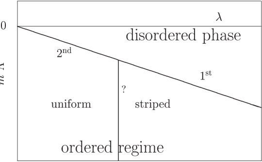
This leads to an ordered phase where the translation invariance is broken spontaneously. In this phase varies in space, which implies the ground state to involve some non–uniform patterns like stripes. These patterns depend on the momentum mode which drives the phase transition. In Ref. [27] these results are summarized in a qualitative phase diagram in the – plane, where is a momentum cut–off.
In Section 2.2.1 we have seen that only the interaction term depends on the parameter . Therefore increasing the coupling also amplifies effects of non–commutativity. According to Ref. [27] the phase diagram in the – plane is then given by Figure 2.2.
A similar phase structure was conjectured in three dimensions. In two
dimensions it was argued that a striped phase does not occur. Gubser
and Sondhi worked with an action of the Brazovskiian form
[28], which is local. Hence the Mermin–Wagner theorem
[29, 30, 31] applies, which
states that spontaneous breakdown of a continuous symmetry is not
possible in two dimensions.
We come back to this point in Chapter 6.
In another approach renormalization group techniques were used to study the phase diagram of the model [32]. Chen and Wu obtained in a new IR stable fixed point, i.e. the non–commutative counterpart of the Wilson–Fisher fixed point. This fixed point is stable, and therefore a striped phase exists, when . In contrast to the results in Ref. [27], this implies that in there is no striped phase. Since we studied the 3d model, we will not address this controversy in this work.
2.3 Non–commutative gauge theory
In this Section we extend our considerations to gauge theories defined on a non–commutative plane.
2.3.1 Star–gauge invariant action
To define a Yang–Mills theory on a non–commutative plane we have to generalize the map (2.5) in Section 2.1 to the algebra of matrix valued functions. Let be a Hermitian gauge field on , which corresponds to the unitary gauge group . We can introduce the Weyl operators corresponding to by taking the trace of the tensor product of and the gauge field
| (2.45) |
where is defined in equation (2.5). Based on equation (2.8) a non–commutative version of the Yang–Mills action can be defined
| (2.46) |
where the term in brackets is the operator analog of the field strength tensor. Here Tr is the operator trace (2.10) and denotes the trace in color space. This action is invariant under transformations of the form
| (2.47) |
where is an arbitrary unitary element of the algebra of matrix valued operators, i. e.
| (2.48) |
The symbol is here the identity on the ordinary Weyl
algebra and is a unit matrix.
To set up the action in coordinate space we can construct an inverse map of (2.45). By mapping the product of matrix valued Weyl operators to coordinate space, using this inverse map, again the star–product (2.16) appears. The Yang–Mills action in coordinate space then reads
| (2.49) |
where we introduced the non–commutative field strength tensor given by
| (2.50) |
The index ’’ indicates that the products in this commutator are
star–products. From equation (2.50) we see that
already for the simple gauge group we have a Yang–Mills type
structure. Therefore there exist three and four point gauge
interactions and non–commutative theory is
asymptotically free.
The invariance under unitary transformations in operator space translates here into an invariance of the action (2.49) under star–gauge transformations given by
| (2.51) |
where is a star–unitary matrix field,
| (2.52) |
Equation (2.52) is equivalent to the unitarity
condition (2.48).
So far we considered non–commutative theories which reduce to the ordinary theories in the limit (on the classical level). In Ref. [33] it was shown that for other gauge groups like this cannot be realized on non–commutative flat space. 222We refer to a constant non–commutativity tensor . The group is closed under the star–product; the product of two star–unitary matrix fields is again star–unitary. In contrast to the special unitary group is not closed, since in general
| (2.53) |
The and the sectors in the decomposition
| (2.54) |
do not decouple in the non–commutative case, because the photon interacts with the gluons [34].
2.3.2 Star–gauge invariant observables
To construct star–gauge invariant observables we consider an arbitrary oriented smooth contour in space–time, which connects the points and . The holonomy of the gauge field over this contour is described by the non–commutative parallel transporter
| (2.55) |
where P indicates path ordering and parameterizes the contour. The index ’’ at the exponential function indicates that in the expansion of this function the star–product has to be used. The parallel transporter (2.55) is a star–unitary matrix field and transforms under the star–gauge transformation (2.51) like
| (2.56) |
A remarkable fact in non–commutative field theory is that space-time translations can be arranged by (star–) multiplication with plane waves
| (2.57) |
where we assume to be invertible. That this equation holds can easily be shown by expanding the exponential functions and using equation (2.19). With the definition of the non–commutative parallel transporter and equation (2.57) we can associate a star–gauge invariant observable with any arbitrary contour by
| (2.58) |
It is straightforward to show the invariance under the star-gauge transformation (2.56) by using equation (2.57) and the cyclicity of the trace over the star–product.
In commutative gauge theory gauge invariant observables can only be
constructed from closed loops. In contrast to that, equation
(2.58) shows that in non–commutative gauge theory we
can find star–gauge invariant observables associated with open
contours. The vector in equation (2.58) can be
regarded as the total momentum of the open loop. This is again a
manifestation of the UV/IR mixing phenomenon, discussed in Section
2.2.2. If we increase the momentum in a given
direction, the contour will extent in
the other directions according to .
This completes our introduction to non–commutative field theories in the continuum. We showed how to define a scalar field theory and a pure gauge theory on a non–commutative plane, and we discussed the main differences compared to the commutative case. This sets up the framework for our numerical studies to be presented in Chapters 4 and 5. In the next Section we will discuss further properties and problems of non–commutative field theory.
2.4 Phenomenological implications of a quantized space–time
In this Section we present phenomenological consequences of a –deformed space–time. To this end we discuss briefly some aspects of the non–commutative standard model.
Gauge fields coupled to matter fields
To set up the non–commutative standard model we have to extend our considerations in Section 2.3 to the case where the gauge field couples to matter fields. We start from the action of a free Dirac field
| (2.59) |
where we extended the commutative theory to a non–commutative theory by replacing the usual products of fields with star–products. The Grassmann valued fermionic fields are represented by . To obtain an action that is invariant under the star–gauge transformations
| (2.60) |
with a star–unitary matrix field , we have to modify the kinetic term of the action (2.59). We follow here Ref. [35] and introduce, in analogy to the commutative case, the covariant derivative
| (2.61) |
where is the gauge field that generates the unitary group . The derivative (2.61) is covariant under the star–gauge transformation (2.51),
| (2.62) |
Replacing the derivative in (2.59) by the covariant derivative leads to the star–gauge invariant fermion action
| (2.63) |
The complete action is then given by the sum of the gauge action
(2.49) and the fermion action
(2.63)
| (2.64) |
As we mentioned in the last Section, it was so far not possible to formulate a non–commutative field theory for the special unitary group . The gauge group is restricted to , which is (for ) not a gauge group of the standard model. There are attempts to modify the space–time non–commutativity in order to take also gauge groups into account [36, 37], but this is an ongoing field of research. However, we may consider the star–unitary gauge field coupled to fermions as an extension of commutative QED.
About renormalizability
The UV/IR mixing poses severe problems for the renormalization of perturbation theory, which are not overcome yet. For instance, scalar fields can become unstable — tachionic — due to IR effects as the non–commutativity is switched on. The attempts to renormalize perturbation theory include methods known from standard field theory [38], the application of Wilson’s renormalization group technique [39, 40, 41], controlling the IR divergences in the framework of supersymmetry [42, 43] and the Hartree–Fock method [27].
In spite of some plausibility arguments in favor
of perturbative renormalizability, it is an open question if
non–commutative quantum field theories do really have finite UV and IR
limits. There are even claims that basic non–commutative field
theories, like non–commutative QED, are not renormalizable
[44].
Violation of Lorentz symmetry
Since carries Lorentz indices, two distinct types of Lorentz symmetries have to be considered [45]: the observers Lorentz transformation and the particle Lorentz transformation. The action (2.64) as well as the scalar action (2.29) are fully covariant under rotations or boosts of the observers reference frame, because and the fields transform covariantly. This does not hold anymore in the case of rotations or boosts of a particle [46]; is unaffected by these transformations. 333The non–commutativity tensor plays the role of an inverse background field (see introduction). From this point of view the Lorentz symmetry breaking occurs very naturally. The symmetry would be restored in a formalism that transforms the particle fields as well as the background field.
The broken Lorentz symmetry implies a deformed dispersion relation, where the deformation depends on the theory under consideration. In the case of the non–commutative theory the dispersion relation is given by the poles of the irreducible two–point function (2.43). We focus here on the case with two commuting and two non–commuting directions. The on–shell condition then reads
| (2.65) |
where is the momentum that corresponds to the non–commutative plane and corresponds to the commutative space coordinate. We include here only the leading IR divergence in first order of ; in addition there is also a logarithmic divergence.
Phenomenology of non–commutative space–time
The effects of non–commutativity on quantities that are measurable in
experiment are studied intensively by many authors. These studies may
be interpreted as an attempt to set stringent limits on the
non–commutativity parameter , or to suggest possibly
measurable effects of non–commutative space–time. We will present
here an
incomplete list of current investigation in this field.
Deformed dispersion relation in gauge theories
Also in gauge theories Lorentz symmetry is broken, which leads to a deformed dispersion relation and changes the particle propagation. This was studied for example in Refs. [47, 48]. There a dispersion relation for photons was obtained containing a term as in the scalar case. Based on one loop perturbation theory the authors of Ref. [47] obtained the photon dispersion relation
| (2.66) |
where they chose the time to be commutative. The coefficient depends on the number of bosonic and fermionic degrees of freedom present in the theory and is the coupling constant.
This may give rise to experimental verification of quantized space–time. The non–linear term in leads to a vacuum dispersion of light, such that the speed of light depends on the wave length. In addition the dispersion depends on the polarization of the photons leading to birefringence.
The authors of Ref. [49] suggest to measure this deformation of the dispersion relation by so–called time of arrival measurements. In these measurements the time delay between photons with different wave length, emitted simultaneously up to a known precision, is measured. The delay will depend on the time the photons are traveling. This effect is (if existent at all) very small. Therefore the sources of the photons should be far distant to accumulate the delay to a measurable effect.
There are attempts by experimentalists to study this effect. Already in high precision measurements 444The accuracy in this measurements was , where is the time delay and is the overall time. of an energy dependent speed of light were performed [50]. However, up to a given sensitivity these measurements did not show any energy dependence.
Newer experiments might give more insight. For example the HESS
project [51], just started to take data, has a higher
sensitivity than in Ref. [50]. Besides other
projects, this collaboration intend to make measurements related to
the vacuum dispersion [52]. Another candidate for
measuring such effects is GLAST [53], which is
expected to start
measurements by the year 2005.
Threshold anomalies
It is still an open question why high energy photons (TeV) from far distant galaxies can be detected on earth [54]. Photons in this energy range traveling over galactic distances should interact with the cosmic microwave background, producing electron positron pairs
The threshold for this reaction is approximately TeV [55, 56] and it should make the observation of high energy photons very unlikely.
A second threshold exist for cosmic high energy protons. There the interaction of the protons with the cosmic microwave background leads to
The protons loose energy when producing pions and the threshold, i.e. the GZK threshold, for this process is at approximately eV [57, 55] Therefore
cosmic protons with higher energy should not be observed. However,
cosmic proton
rays have been detected beyond this limit [58].
In both cases non–commutative space–time could provide an explanation of these anomalies. The thresholds can be estimated kinematically using the momentum and energy conservation. In a Lorentz invariant theory the threshold momentum in the case of high energy protons is approximately [59]
| (2.67) |
where and are the masses of the proton and of the pion,
respectively, and is the energy of the background photon that
interacts with the proton. In a non–commutative space–time the dispersion
relation is given by equation (2.66). Inserting
the deformed dispersion relation into this computation
leads to a
dependent threshold.
Bounds on
So far we discussed new effects and known problems that might be explained by non–vanishing . Let us now address the limits on set by existing experiments and the possibility of setting bounds on in near future experiments.
The fact that in the aforementioned time of arrival measurements no
energy dependence was measured, allows to set a lower limit on
(if we assume a non–zero from the beginning).
Note that here we find a lower limit, because the
dispersion relation (2.66) implies that larger
values of correspond to a softer deformation of the standard
dispersion.
555The rather unexpected lower bound of is related
to the order of UV limit and commutative limit, as we discussed in
Section 2.2.2. This lower bound can be understood in
the sense that if there is a non–commutative space–time,
then has to be larger than a certain value. However, this
does not exclude .
On the other hand if one wants to solve the cosmic proton threshold
anomaly within the framework of non–commutative field theory one
finds an upper bound of . According to Ref. [47] this leads to a rough estimation of the
a parameter in the range
.
More precise bounds on could be obtained from accelerator physics. Since non–commutative QCD is not well formulated yet, these investigations are restricted to measurements described by QED. Hence one expects the most significant results from linear colliders.
The idea is to compute for example cross sections for scattering processes from the standard model and from the non–commutative standard model [60]. 666The calculations in non–commutative QED rely on the Feynman rules developed in Ref. [34, 61, 62, 63]. This leads to different predictions for the two models, where both predictions depend of course on the center of mass energy . Measurements of these observables then may verify the non–commutative picture or set an upper bound on . Measurements in existing colliders did not show any signal of non–commutative space–time. Therefore one is looking for search limits, which can be probed in future colliders (TESLA [64], NLC [65] and CLIC [66]) .
| process | search limit on at TeV |
|---|---|
| pair production | GeV |
| Compton scattering | GeV |
For example, Ref. [67] reports search limits for the
processes listed in Table 2.1 on the basis of
the design of these colliders. Further search limits can be found for
example in Ref. [68]. For recent reviews concerning
the activities in this field see
for example Ref. [69, 70, 71].
Note that the theories, which the above presented results are based on, still suffer from IR divergences. They are obtained from one loop calculations. Higher orders in perturbation theory are not under control yet. It is still an open question if the non–commutative field theories are renormalizable in two or three loop calculations. The limits on were obtained assuming that higher order correction will not change the results qualitatively. However, one cannot exclude dramatic changes coming from higher loop contributions.
2.5 Summary
Let us briefly summarize the effects of non–commutative space–time on field theories defined on it. We showed that introducing non-commutativity via the commutation relation (2.2) leads to a non–commutative and non–local product, i.e. the star–product. Field theories may be formulated on this geometry by replacing all products in the commutative theory by the star–product of the fields. This results in a non–local action. In a perturbative treatment one discovers a mixing of high and low energy effects. The UV/IR mixing causes serious problems in perturbative renormalization, since some of the UV divergences in commutative theories turn into IR divergences in the non–commutative model even in the massive case. We discussed this new effect in one loop perturbation theory. Already there the divergences at low momenta cause enormous problems. The difficulties increase when these loops are sub–loops of a higher order contributions.
In a –deformed space–time the Lorentz symmetry is explicitly broken. This leads to unexpected particle propagation like a momentum dependent speed of light. These effects are the most likely candidates for experimental verifications.
In non–commutative gauge theories the gauge symmetry turns into a
star–gauge symmetry. This allows us to construct star–gauge
invariant observables that are associated with open Wilson loops. The
open loops carry a momentum proportional to the separation between the
endpoints. This is again a UV/IR mixing effect. In non-commutative
QED the photons interact, which might again give rise for new
measurable effects.
As an alternative to perturbation theory we are studying non–commutative field theories in the lattice approach [72]. This work has to be considered as the beginning of a long term project. At the end of this project we want of course to compute phenomenological quantities, but in the starting phase we will study field theory in lower dimensions in order to understand better the non–perturbative treatment.
However, already the study of these toy models gives insights into the four dimensional theory. Since also for these models there exist perturbative results, it is an interesting question if in a non–perturbative study new effects arise and how far perturbation theory can be confirmed.
Chapter 3 Lattice regularization
As we have seen in Section 2.2.2, introducing non-commutativity of space–time does not cure the ultraviolet divergences occurring in the commutative case. Therefore the field theories still have to be regularized, by introducing a momentum cut–off. In this Chapter we discuss the lattice regularization. For a more detailed discussion we refer to Refs. [73, 74, 25, 26, 75].
3.1 Discrete non–commutative space–time
On the cubic lattice the space–time points are restricted to discrete values , where is the lattice spacing. Here momentum space is compact and the momenta must be identified under the shift
| (3.1) |
As in the continuum, non-commutativity comes into the game by replacing the ordinary coordinates by Hermitian coordinate operators , which satisfy the commutator relation (2.2). As a consequence of equation (3.1), we can set up the operator identity
| (3.2) |
By multiplying both sides of equation (3.2) with we find
| (3.3) |
where is again the identity of the algebra of Weyl operators. The usual constraint of lattice field theory that the discretization has to be compatible with the spectrum of the position operator leads to
| (3.4) |
Moreover we find an additional constraint for the momenta
| (3.5) |
Combining this result with the periodicity in momentum space (3.1) implies that is an integer for all , leading to a discrete momentum
| (3.6) |
The periods are integer multiples of the lattice spacing and the periodicity (3.1) can be expressed by the integers via .
Due to the discrete momentum space the space–time coordinates are restricted to a periodic lattice
| (3.7) |
Therefore the lattice regularization forces space–time to be compact. The discrete compactification is a non–perturbative manifestation of the UV/IR mixing effect; the perturbative manifestation was described in Section 2.2.2. For practical applications this means that systematic errors resulting from the finite lattice spacing are always entangled with finite volume errors.
The continuum limit does not commute with the commutative
limit . Taking first the continuum limit restores the
infinite space–time , while taking first the
commutative limit shrinks the space–time lattice to a single point as
one infers from equation (3.5).
Due to the momentum discretization (3.6) we cannot use the unbounded operators . Instead we have to use the unitary coordinate operators , which have been introduced in Section 2.1.3
| (3.8) |
These operators generate the algebra of functions on a non–commutative torus 111Note that in equation (3.9) and (3.12) no sum over is taken.
| (3.9) |
where the dimensionless non-commutativity tensor is defined as
| (3.10) |
Moreover since we are dealing with a discrete torus, one should rather use the shift operator
| (3.11) |
instead of the linear derivative (defined in (2.6)). This operator effects translations in units of the lattice spacing
| (3.12) |
The algebra defined in (3.9) and (3.12)
replaces the algebra
based on (2.2) and (2.6).
Now we consider scalar functions on a non–commutative discrete torus, where we assume that these functions may be expressed by a discrete Fourier transformation of . Lattice Weyl operators are then defined by the formal Fourier transform
| (3.13) |
analogous to the continuum (2.4). The relation between the integer vector and the momentum is given by equation (3.6). Replacing in equation (3.13) by its Fourier transform and using equation (3.9) leads to an explicit map between operators and fields
| (3.14) |
This map is the lattice analog of the continuum map (2.24). Here is a point on the space–time lattice . The map between fields and operators then reads
| (3.15) | |||||
| (3.16) |
where the operator trace is uniquely given by
| (3.17) |
3.2 Non–commutative field theory on the lattice
With the definitions of the last Section it is straightforward to construct field theories on a non–commutative lattice. In the case of a scalar theory we use the map (3.15) to define the operators . The action in terms of Weyl operators then reads
| (3.19) |
where is the lattice shift operator defined in equation (3.11) . Using the inverse map (3.16) leads to the lattice action of the field
| (3.20) |
where is the unit vector in the direction . Since also the lattice version of the star–product is invariant under cyclic permutation, only the interaction term differs from the commutative case, as in the continuum.
To construct a non–commutative Yang–Mills theory on the lattice we need the non–commutative counterpart of the link variables . In order to preserve star–gauge invariance the link variables have to be star–unitary. This can be formally achieved by taking the parallel transporter defined in (2.55) between the lattice sites and
| (3.21) |
where is a non–compact gauge field and indicates that in the expansion of the exponential function the star–product has to be used. is star–unitary and transforms under star–gauge transformations as
| (3.22) |
where is again a star–unitary matrix field introduced in equation (2.52). The corresponding Weyl operators are given by
| (3.23) |
The star-unitarity of the link variables is now equivalent to unitarity of the Weyl operators.
The action of a non–commutative Yang–Mills theory can again be constructed with the use of the lattice shift operators (3.11) or with the star–product
| (3.24) |
where is the trace in the fundamental representation of the
unitary group .
As in the continuum we find in coordinate space a simple recipe to construct a field theory on a non–commutative plane: replace all usual products in the commutative theory by star–products. In this spirit we now define star–gauge invariant observables in non–commutative lattice gauge theory, by replacing the products in the commutative Wilson lines with star–products
| (3.25) |
Here is an arbitrary lattice contour with the displacement vector between the two end point of the contour. In the commutative case the trace over these lines is gauge invariant if the lines are closed, either on the plane or over the boundary. This implies or , respectively, where indicates how often the contour winds around the torus in the -th direction.
On the non–commutative torus we can construct star–gauge invariant observables for any separation vector by multiplication by plane waves
| (3.26) |
where the relation between the momentum , carried by the contour, and the separation vector on the torus is given by
| (3.27) |
The fact that open loops carry a momentum proportional to the separation vector again displays the UV/IR mixing.
3.3 Matrix model formulation
In the last Section we constructed a scalar and a pure gauge action on a non–commutative lattice in terms of Weyl operators and in terms of functions with a deformed product, i.e. the star–product. The latter allows for an intuitive extension from commutative field theories to their non–commutative counterparts and it may seem to be suitable for a direct simulation. However, from a practical point of view this formulation rises enormous problems for Monte Carlo simulations.
Already in the scalar case we have to implement the lattice version of
the star–product, which involves a sum over the complete lattice for
every product. This increases the needed computer time to an almost
unreachable amount. In addition to this, in gauge theory we have to
construct star–gauge invariant link variables , which makes the
simulation even more expensive. To avoid these problems we will use a
finite dimensional representation of the operator description.
Here we are leaving the general discussion and restrict ourselves to the case that we studied numerically. This is a 2d non–commutative space or subspace with the period matrix given by
| (3.28) |
where is the lattice spacing on a hyper–cubic lattice and is the number of lattice sites in each direction. Then the coordinate operator (3.8) and the dimensionless non-commutativity tensor (3.10) are given by
| (3.29) |
The quantization of momentum and the non–commutativity parameter read
| (3.30) |
The algebra (3.9) then simplifies to
| (3.31) |
where is the totally antisymmetric tensor.
The key step is now to replace the operators and in the algebra (3.9) by matrices, satisfying the relations (3.31). For odd values of there is a simple choice to achieve this, given by the so–called twist eaters . In two dimensions this amounts to
| (3.32) |
where we introduced the twist in a way that will be useful in the next Section. Inserting (3.32) in (3.31) fixes the twist to
| (3.33) |
The equations (3.32) are of course only one possible choice. For a general construction see for example Refs. [73, 25, 76].
With these definitions an explicit form of the star–product (3.18) is provided and the operator becomes a matrix
| (3.34) |
The map between the functions and the matrices in terms of then reads
| (3.35) |
where the trace now refers to the matrices. If we insert explicitly in the left equation of (3.35) we obtain the matrices . Since the Fourier transform of is given by
| (3.36) |
the matrices read
| (3.37) |
and we obtain a map between Weyl operators and the Fourier transform .
| (3.38) |
Chapter 4 Numerical studies of non–commutative gauge theory
In this Chapter we present the results of our studies of 2d non–commutative gauge theory. As already discussed in the previous Chapter the lattice version of non–commutative gauge theory in coordinate space (3.24) is not immediately suitable for computer simulations. Therefore we make use of the finite dimensional representation introduced at the end of the last Section. The model we will arrive at is the twisted Eguchi–Kawai model (TEK). We start with a discussion of the origins of this model.
4.1 The twisted Eguchi–Kawai model
4.1.1 History of the TEK
In 1982 Eguchi and Kawai conjectured that standard (commutative) and lattice gauge theory in the large limit is equivalent to their dimensional reduction to (one point) [77]. The link variables are replaced by , and the partition function of the Eguchi–Kawai model (EK) simplifies to
| (4.1) |
where . Eguchi and Kawai proved that in the large
limit both models have the same Schwinger–Dyson equations — and
therefore the same Wilson loops — if the global symmetry of
the phases is not spontaneously broken. In this symmetry is
unbroken and the equivalence holds exactly, but in this is not
the case anymore. There the equivalence holds only at
strong coupling [78].
A way out of this restriction to two dimensions is using twisted boundary conditions rather than periodic ones [79]. It is known that the behavior of the partition function at weak coupling differs significantly between twisted and periodic boundaries. Therefore one can expect that the symmetry breaking at weak coupling could be cured.
To obtain the twisted Eguchi–Kawai model one applies the transformation
| (4.2) |
to the partition function with the standard Wilson gauge action [72]
| (4.3) |
The ’s can in general depend on space–time, but for the purpose here it is enough to keep just the dependence on the orientation. The integration measure is invariant under this transformation and the transformed action reads
| (4.4) |
The twist is the product of the factors at the boundary of the plaquette. It can be characterized by an integer valued anti–symmetric matrix
| (4.5) |
Neglecting the space–time dependence of the link variables then defines the TEK action
| (4.6) |
and a general Wilson loop spanned by plaquettes is given by
| (4.7) |
In Ref. [80] it is shown that with this action the equivalence between the TEK and commutative and lattice gauge theory also holds in .
Here we are concerned with the 2d TEK. It seemed for a long time
that adding a twist is not highly motivated in , since there
even the ordinary EK model coincides with lattice gauge theory
in the planar large limit, which was solved analytically
by Gross and Witten [81].
However, the situation changed suddenly due to a new interpretation of the TEK as an equivalent description of non–commutative gauge theory [82]. This equivalence was established by embedding the (dynamically generated) coordinates and momenta of the reduced model into matrices. These matrices can be mapped on functions, where the trace turns into an integral and the star products arise, so that one arrives at action (2.49). The construction of non–commutative gauge theories (for certain ) works out in this way at . 111Note that is here the size of the matrices , whereas refers to the gauge group . At finite the conditions cannot be matched at the boundaries.
4.1.2 TEK at finite
An interpretation of the TEK at finite occurred when Refs. [73, 74, 25] pointed out that the twisted reduced model can be mapped exactly on a non–commutative lattice gauge theory 222Remember that gauge theories so far cannot be constructed on a non–commutative plane and therefore this equivalence exists only for gauge theories. in general dimension and rank of the gauge group. Here we will describe the case of and the star–unitary gauge group .
To show the equivalence we will use the finite dimensional representation of a non–commutative geometry, developed in Section 3.3. The starting point is the action of 2d non–commutative lattice gauge theory in terms of operators (3.24)
| (4.8) |
Inserting the finite dimensional representation (3.34) of the general shift operator leads to
| (4.9) |
The twist eaters obey the Weyl–’t Hooft commutation relation
| (4.10) |
The substitution in equation (4.9) along with the commutation relation (4.10) for the inner ’s leads to the TEK action (4.6).
In this representation the twist reads
.
Comparing this with the twist needed for the TEK, where the exponent
is given by multiplied by some integer, we find that
has to be fulfilled. Therefore we have to use
odd values of .
Note that this interpretation of the TEK differs significantly from the original one. While in the original interpretation the space–time degrees of freedom become irrelevant in the large limit, in the interpretation here the space–time degrees of freedom are exactly mapped onto matrix degrees of freedom already at finite .
4.1.3 Continuum limits
The continuum limit also requires the limit , where the order of these limits is important for the resulting continuum theory.
The planar limit
In the planar limit one first sends , keeping the lattice spacing fixed, followed by the continuum limit along with in a particular way dictated by the coupling constant renormalization. Equation (3.30) implies that in this limit and only planar diagrams remain. In there exists an exact solution of planar and [81]: rectangular Wilson loops follow the area law
| (4.11) |
where is the expectation value of the Wilson loops. The string tension is given by
| (4.12) |
Equation (4.11) shows how the bare coupling has to be tuned as a function of when one takes the continuum limit. In this case the scaling is exact if one identifies the lattice spacing as
| (4.13) |
The double scaling limit
In the double scaling limit one takes the thermodynamic limit and the continuum limit at the same time keeping fixed. Here we used the relation (3.30) between and the lattice spacing. This leads to a finite non–commutativity parameter in the continuum limit and one recovers non–commutative 2d theory in .
This is the continuum limit we studied. has to be scaled as a function of the lattice spacing in exactly the same way as in the planar theory. From equation (4.12) we read off at large . Hence in we are going to search for a double scaling limit keeping the ratio constant. The question of renormalizability of 2d non–commutative gauge theory at finite can be answered by studying this large limit of the TEK. If the observables converge to finite values, we can conclude that 2d lattice non–commutative gauge theory does have a finite continuum limit. Our results will be presented in the next Section.
4.2 2d non–commutative theory
4.2.1 The model
We study the double scaling limit in two dimensional non–commutative lattice theory. The explicit action in terms of dimensionless quantities reads
| (4.15) |
with the twist given by (3.33). If not stated differently
we set .
For details of the simulation see Appendix A.2.
Our main interest in this model is whether a finite continuum limit exists or not. Thus we study the double scaling limit — as described in the previous Section — of various observables. If we find a large scaling of these observables (at fixed ) this corresponds to a finite continuum limit.
The observables we measure are constructed from Wilson loops spanned by plaquettes
| (4.16) |
and from open Polyakov lines,
| (4.17) |
where is the number of multiplied link variables and indicates the backward direction.
In Section 3.2 we showed that one can construct star–gauge invariant observables from general open lines. Here we restrict ourselves to straight lines which are not necessarily closed by the boundary.
4.2.2 Wilson loops and area law
First we study the expectation values of Wilson loops. The expectation value of open Polyakov lines is vanishing. In fact the expectation value of any open contour vanishes due to the symmetry of the TEK. But –point functions of these contours are sensible observables.
In the EK model it was observed that square shaped Wilson loops converge faster to the known exact result than other rectangles with the same area [84]. Hence we also focus on square shaped Wilson loops, which corresponds to in the definition (4.16). We define the normalized Wilson loop
| (4.18) |
Due to the presence of the twist, there is no invariance under the transformation , . As a consequence is in general complex and , hence the Wilson loop depends on the orientation. The real part represents the average over both orientations.


Figure 4.1 shows the real part of the Wilson loops as a function of the physical loop area.
Large scaling is clearly confirmed. At small up to moderate areas the Wilson loop follows the area law of planar lattice gauge theory given in Eq. (4.11), but at large areas it deviates and the real part oscillates around zero instead. This observation is consistent over a wide range of . Remarkably, not even the absolute value decays monotonously; at large areas it seems to fluctuate around an approximately constant value. This is illustrated in Figure 4.2 (top).
Figure 4.2 (below) shows that beyond the Gross–Witten regime, the phase increases linearly in the area. Additional measurements at , corresponding to different values of , are shown in Figure 4.3. They reveal that the phase of the Wilson loop is, in fact, given the simple relation
| (4.19) |
where the area is given by . This relation holds to a high accuracy at large areas , i.e. beyond the Gross–Witten regime. Relation (4.19) has been confirmed also for other (non–square) rectangular Wilson loops, which shows that the effect does not depend on the shape of the Wilson loops. 333Note, however, that the expectation values of Wilson loops with the same area but with different shapes have in general different absolute values in the double scaling limit. Indeed the formula (4.19) agrees with a Aharonov–Bohm effect in the presence of a constant magnetic field across the plane. This is reminiscent of the description of non–commutative gauge theory by Seiberg and Witten [8]. This interpretation is also known in solid state physics. Our numerical results seem to support a picture of this kind.
The observed large area behavior of the Wilson loops confirms that the continuum limit of non–commutative gauge theory is different from any ordinary gauge theory, hence we have found a new universality class. Since the non–locality in this model is of order , one might naively think that in the large area regime, , the effect of non–commutativity is invisible. The fact that we the observe contrary can be understood as a manifestation of non–perturbative UV/IR mixing.
In the two dimensional model there is no perturbative UV/IR mixing,
since there are no UV divergent diagrams in the commutative case. Here
we found this mixing at a completely non–perturbative level.

In the double scaling limit of the untwisted Eguchi–Kawai model, the expectation values of the Wilson loops is real, and it remains positive even at large areas [84]. This means that the two models, twisted and untwisted, yield qualitatively different double scaling limits, although they become identical in the planar large limit.
4.2.3 2–point functions
Here we consider 2–point functions. Figure 4.4 (top) shows the connected Wilson loop 2–point function
| (4.20) |
again plotted against the physical area, for . In contrast to the Wilson loop itself, is a real quantity, since both orientations of the Wilson loop are involved.
In Figure 4.4 (below) we include a wave function renormalization factor
| (4.21) |
The exponent was found to be optimal for to scale.
Indeed it leads to a neat large scaling over more than two
orders of magnitude in the physical area.
Next we consider the Polyakov line
| (4.22) |
which is also invariant and therefore has an interpretation as a star gauge invariant observable in non–commutative gauge theory. Their momentum is related to the separation vector between the two ends of the line. In general the relation is given by modulo the periodicity of the torus, as discussed in Section (3.2). In the present case, the Polyakov line corresponds to a momentum mode with , where the integer is given by and by for even and odd , respectively. In the following, we plot our results against the physical distance for even .
The phase symmetry 444In the terminology of non–commutative gauge theory, this corresponds to momentum conservation. makes vanish, but the connected -point functions () of Polyakov lines are sensible observables. In Figure 4.5 we show the 2–point function 555The choice of the direction is irrelevant. In practice we average over both possibilities in order to enhance the statistics.


| (4.23) |
Note that there is no disconnected part in . Again we insert the wave function renormalization which was optimal for the Wilson 2–point function
| (4.24) |


As a function of the physical length , the result is consistent
with large scaling, as well as a universal
wave function renormalization.
A similar wave function renormalization was also observed in the
EK model [84], where the optimal factor in
relation (4.24) is modified to .
The large scaling of the Wilson loops as well as the large scaling of 2–point functions of Wilson loops and Polyakov lines, described in this Chapter, correspond to a finite continuum limit in 2d non–commutative gauge theory. This observation therefore demonstrates the renormalizability of 2d non–commutative theory.
Chapter 5 Numerical studies of the model
The second model we investigated is the 3d non–commutative theory. In Section 2.2 we described the effects of the UV/IR mixing effect based on results of one loop calculations. We studied this model non–perturbatively and in this Chapter we present our results. For details of the simulations we refer to Appendix A.3.
5.1 Dimensionally reduced model
Since we are in odd dimensions we cannot apply directly the construction of non–commutative field theories as described in Chapter 2 and 3. There the anti–symmetric non–commutativity tensor had to be invertible. This restricts the dimension to be even.
In addition to this rather technical problem related to odd dimensions, a non–commutative time could give rise to unitarity problems [85, 86]. Ref. [87] showed that field theories on a non–commutative space satisfy the generalized unitarity relations. If the time is also non–commutative this is not the case. Therefore we exclude the time direction from non–commutativity. 111In four dimensions the problem is often avoided by taking two commuting and two non–commuting directions.
Then the non–commutativity tensor is two dimensional and acts only in the 2d non–commutative subspace. The star–product defined in (2.16) then reads
| (5.1) |
and the lattice version of the star–product is analogous. Here means , where satisfy the commutation relation (2.18) and commutes with all coordinates.
The corresponding Weyl operators then also depend on the time and the lattice action of this version of non–commutative theory reads, in analogy to equation (3.19),
| (5.2) |
where . There are now two kinetic terms: the first one uses the shift operators (3.11) to perform spatial translations in units of the lattice spacing . The second kinetic term is the square of the standard discrete derivative in time direction.
As in the TEK model we use here the finite dimensional representation (3.32). In this representation the Hermitian operators turn into Hermitian matrices and the shift operators are replaced by the twist eaters .
Effectively we are mapping here a non–commutative lattice theory, defined on a three dimensional lattice, to a one dimensional lattice with sites.
On each site
there is a Hermitian matrix representing
the Hermitian operators, see Figure 5.1. We
use periodic boundary conditions . In
our simulations we always set
.
The dimensionless parameters and in the action (5.2) can be identified with physical parameters
| (5.3) |
Here we used the relation between the non–commutativity parameter and the lattice spacing (3.30). With this identification the double scaling limit described in Subsection 4.1.3 leads to the non–commutative model on . In this procedure the limits and are taken such that is kept constant, leading to a finite non–commutativity parameter.
Here we will not study the continuum limit and the question of
renormalizability. Instead we study the phase diagram and the UV/IR
mixing effects in the regularized theory.
In Section 2.2.2 we discussed this issue in . Since the results depend on the dimension, we repeat the considerations of Section 2.2.2 for the case of three dimensions.
We start with the non–planar one loop contribution to the irreducible two–point function in equation (2.44). In this term reads
| (5.4) |
where is again a momentum cut–off and . Since we chose the time as commutative, only the spatial components of the momentum appear here. Introducing the effective cut–off as in equation (2.38)
| (5.5) |
and evaluating the Bessel function leads the one loop corrected two–point function
| (5.6) |
with . As in Ref. [4] we absorbed the planar contribution into the effective mass . After removing the cut–off in equation (5.6) we obtain the leading IR divergence
| (5.7) |
Again the two–point function is singular at zero momentum. However, here is not a function of , which leads to a different IR behavior of the theory.
5.2 The phase diagram
As we discussed in Section 2.2.3 the phase diagram of the non–commutative 3d theory is expected to differ significantly from the phase diagram in the commutative case. In this Section we present our Monte Carlo results for this phase diagram.
5.2.1 The order parameter
When studying a phase diagram one first has to identify a suitable order parameter that indicates the symmetry breaking. In the model here we expect an Ising type phase, where the discrete symmetry is broken spontaneously. In addition we expect — for sufficiently large coupling — a striped phase, where the translation symmetry is broken spontaneously (see Section 2.2.3). Therefore we need an order parameter that is sensitive to both variants of symmetry breaking, to distinguish the two types of ordered phases.
The momentum dependent quantity
| (5.8) |
turned out to be a good choice. The vector is the integer representation of the momenta introduced in equation (3.6). Here is the spatial Fourier transform of the field , where only the non–commutating coordinates are transformed. The expectation value of is zero in the disordered phase, where both symmetries under consideration are unbroken. In an Ising type or uniform phase only the expectation value of is non–zero, since
| (5.9) |
is the standard order parameter of the spontaneous breakdown of the symmetry. A non–vanishing order parameter at indicates a spontaneous breakdown of the translation symmetry and therefore it implies the striped or non–uniformly ordered phase.
Since we are simulating the dimensionally reduced model in terms of the matrices we have to express this order parameter by these matrices. To this end we use the map defined in equation (3.38) and we obtain
| (5.10) |
This order parameter detects the disordered as well as the uniformly ordered phase. In the striped phase there will arise problems when the pattern for different configurations are rotated. For example if there are stripes for one configuration parallel to the and for another configuration parallel to the there would be two different non–vanishing order parameters. This effect is related to the rotation symmetry, which is also broken spontaneously in the striped phase. 222Actually rotation symmetry is explicitly broken on the lattice. However, in the commutative case this symmetry is reduced to an invariance under rotations of , which can be broken spontaneously in the non–commutative lattice theory. To avoid this problem we defined the rotation invariant order parameter as the expectation value of
| (5.11) |
This order parameter depends only on the absolute value of the momentum
and therefore the above mentioned problem does not occur. Based on
this order parameter we explored the phase diagram of the 3d
model.
5.2.2 Numerical results
With the algorithm described in Appendix A.3 we generated configurations at various values of , and and measured the order parameter (5.11). The result is the phase diagram plotted in Figure 5.2. The points connected by lines display the phase transition between disordered phase and the ordered regime.
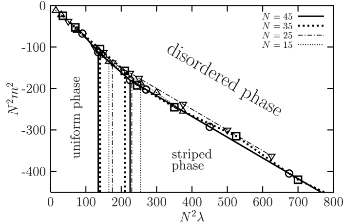
The ordered regime clearly splits into a uniform and in a striped phase, where the transition region between these two phases is marked by two vertical lines for each value of . For each the left line represents the largest value of at which we are still in the uniform phase, and the right lines show the smallest value of , where we are already in the striped phase. Both transitions stabilize in if we multiply the axes by .
To illustrate the different phases we mapped the matrices back to coordinate space () using the map (3.34). We chose configurations in the four areas that can be distinguished.

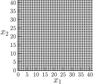
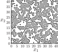

Some example snapshots of are shown in Figure 5.3. The dotted areas indicate and in the blank areas is negative. Figure 5.3(a) and 5.3(c) show in the disordered phase. The positive and negative areas are spread all over as one expects in the disordered phase. Also in the uniformly ordered phase we find the expected behavior; is either positive for all or negative for all (Figure 5.3(b)).
Figure 5.3(d) shows a typical pattern with two stripes.
In the range of the parameters plotted in the phase diagram
5.2 we always found two stripes (in the
non–uniformly ordered phase). They were either parallel to the or to the
axis. We will discuss the number of stripes separately in the
next Subsection. In the rest of this Subsection we discuss the
measurements that
the phase diagram 5.2 is based on.
To localize the phase transitions we started simulations in the disordered phase. After we reached equilibrium we measured . Then we decreased slowly towards the expected phase transition.
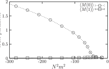
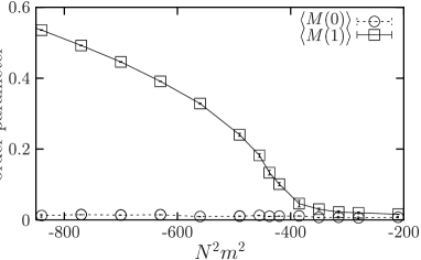
Figure 5.4 shows two example measurements at . We plotted in both cases the order parameter at and against . On the left we started in the disordered phase at . Below a critical value of , we see a clearly non–vanishing at , while is zero for all values of . This indicates that we are entering the uniform phase. On the right we started in the disordered phase at . Lowering leads to a non–zero order parameter at and the standard order parameter is zero. The fact that implies that the system is in the striped phase.
Measurements of this kind allowed us to separate the uniform phase from the striped phase. 333A natural method the determine the transition line between uniform and striped phase is to start in the uniform phase and increase or vice versa. However, it turned out that the initial patterns remain stable when the transition region is crossed. Whenever we see a dominant order parameter with we are in the striped phase. Unfortunately we were not able to determine an accurate transition line between these phases. We obtained a transition region, in which it was not possible to identify the order of the system. Depending on the starting conditions (see Appendix A) we found indication for both phases. We come back to this point in Section 5.4.
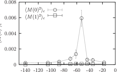
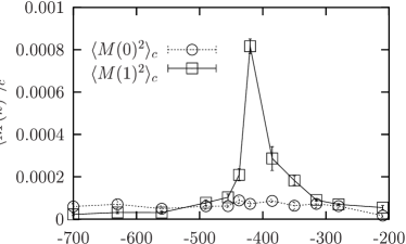
From plots like shown in Figure 5.4 one can also identify the transition line between disordered phase and ordered regime, at least roughly. Whenever any order parameter becomes non–zero we hit the transition line. However, one can localize the transition more accurately by looking at the connected part of the two–point function of ,
| (5.12) |
From statistical mechanics it is known that this two–point function has a peak at the phase transition.
5.2.3 The striped phase
In Figure 5.4 we have seen that the two types of ordered phases can be distinguished by the momentum of the non–vanishing order parameter . We showed the two possibilities . It was left as an open question how behaves for other values of . This we want to discuss here.
In Figure 5.6 we plotted two examples of the order parameter against the momentum , where in both cases we are clearly in the ordered regime. On the left the system is in the uniformly ordered phase. Only the standard order parameter is non–zero, for all other momenta the order parameter is zero. This defines the uniform phase.
The right plot in Figure 5.6 shows the system in the striped phase. There we see again a non–zero order parameter at . In addition we also see a signal for .
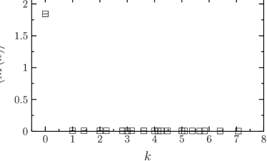
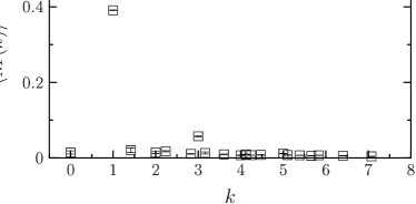
This may appear as an indication for an underlying multi–stripe structure, which is not visible when we plot the sign of , as we did in Figure 5.3. In fact this is not the case. To illustrate this we define the function
| (5.13) |
In this definition we assume that the stripes are parallel to the axis. The function averages over and at . If there is an additional structure 444Of course the method will not find all possible patterns, but we also looked for additional structures in the other direction, which were not present.
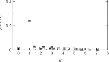
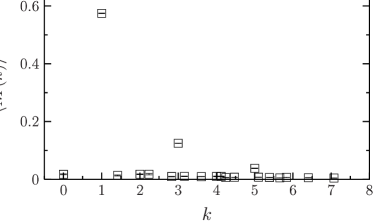
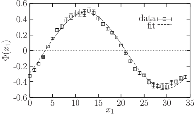
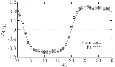
this should be seen in the behavior of . To examine this we first computed the order parameter from configurations close to the phase transition and from configurations at large negative values of . The results are shown in Figure 5.7 (top). On the left the system is close to the phase transition and only is non–zero. On the right, at large negative values of , we see that also and are different from zero. It is evident that when is further decreased, will also be non–vanishing for larger (odd) momenta .
We computed on one configurations in each of these regions, to study how the additional momentum modes influence this function. The results are plotted in Figure 5.7 (bottom). If there is only one non–vanishing mode of the field this corresponds to a pure sine behavior. This is clearly confirmed by the plot on the left. The dashed line is a fit of the data to a sine function. 555The function is an average over and . The errors displayed in Figure 5.7 are computed with respect to this average with the binning method (see Appendix A.1). On the right is plotted in the case of various non–vanishing momentum modes. Here we see that these additional modes do not indicate a more complicated structure. It simply displays that deeply in the striped phase is no more a pure sine, but the Fourier series involves higher momenta. As a fit function in this plot we used the first three odd terms in such an expansion, according to the three non–vanishing modes in Figure 5.7 (right, top), which fits the data perfectly. This result means for the structure of the field that at large negative values of the number of stripes does not change, but the field is here restricted to only two values. At the kinetic term is negligible and the anti–ferromagnetic coupling dominates the system.
As we mentioned above we obtained — in the range of the parameters shown in the phase diagram 5.2 — never more than two stripes. Analytically one expects not only two stripes, but also more complicated patterns [27]. To be in agreement with the perturbative conjecture these complex patterns should also occur on the lattice. The multi–stripe patterns are expected either on larger lattices or at larger non–commutativity parameter or at larger coupling .
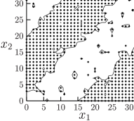
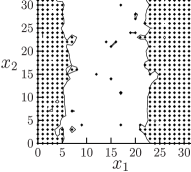
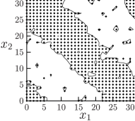
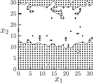
In fact for increased we obtain also diagonal stripes, which support the picture of Gubser and Sondhi. However, only in the continuum limit, where the number of stripes should diverge, this picture can be ultimately verified. Some example snapshots at are displayed in Figure 5.8. The different patterns shown here correspond to different starting configurations. We postpone the discussion of the vacuum until we have considered the dispersion relation.
5.3 Correlation functions
In this Section we present our results concerning the correlation functions. The main interest here is to study the dispersion relation, but also the behavior of two–point functions in position space.
5.3.1 Spatial correlators
There are several predictions about the behavior of the correlation functions in coordinate space in the 4d theory. It is expected from one loop perturbation theory that the decay of this correlator at small is not exponential [4]. For larger the exponential behavior is restored but now depending on the coupling instead of the mass. This refers to the disordered phase. In the non–uniformly ordered phase an oscillation of the correlator is expected. Here we are studying the behavior of these correlators in .
We are dealing here with one commuting and two non–commuting coordinates, namely the spatial coordinates. Since only the correlators in the non–commuting directions are expected to have an exotic behavior, we focus on spatial correlators. To be explicit, we study the correlation function 666In practice we use the twist eaters (3.32), which are a finite dimensional representation of the shift operators (3.11) to compute this quantity. We discuss this issue here and in the following in coordinate space since then the quantities are intuitively readable.
| (5.14) |
In Figure 5.9 the correlator (5.14) in the disordered phase at is shown. We measured the in one direction keeping fixed in the other direction. In Figure 5.9 we averaged over both directions. On the left we plotted the correlator
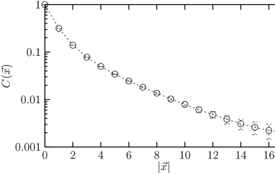
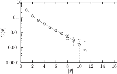
(5.14) at and on the right at . The decay is clearly not exponential at these values of the coupling.
In Figure 5.10 we show results at increased coupling. At moderately enlarged the decay appears almost exponential (on the left),
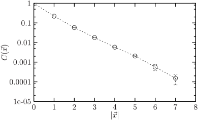
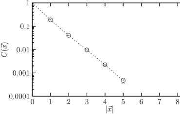
and at very large coupling the exponential decay is restored (on the
right). The non–exponential decay of the spatial correlators was a
result obtained from perturbation theory in four dimension. Here we
observed this behavior in the 3d model.
In the striped phase we have to take more care about the direction in which we measure the correlation function (5.14), since here we have patterns leading to a dependence of the correlator on the direction. Therefore an analysis of the stripe pattern has to be done first. This is achieved by evaluating the order parameter defined in equation (5.8). This order parameter depends also on the orientation of the condensed momentum mode and it is therefore not suitable for detecting the disordered – striped phase transition. However, here it is a perfect observable to detect the patterns. The momentum that maximizes dominates the pattern in the striped phase. For example, a maximum at indicates two stripes parallel to the axis, and a maximum at or at indicates diagonal stripes.
We measured the correlation function parallel and vertical to the stripes separately. For completeness we plotted in Figure
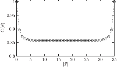
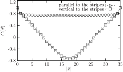
5.11 on the left also an example of
in the uniform phase. In this phase we see a strong correlation as
expected in a uniform phase. However, in the striped phase (on the
right) at the spatial correlator behaves differently in
the two directions. At this value of we obtained two stripes
parallel to one of the axis. Therefore we find in one direction
(parallel to stripes) still a strong correlation. In the direction
vertical to the stripes we see a strong anti–correlation. Since
at this value of the coupling we have only two
stripes, the correlator does not oscillate.
The situation changes if we increase the coupling further. In Figure 5.12 is plotted at and . In the last Section we showed already snapshots of at these values of the coupling. We saw there that depending on the starting configuration we obtain qualitatively different patterns. This leads to a different behavior of the spatial correlator (5.14). Again we refer to Section 5.4 for a discussion. Here we show results for the different striped phases separately.
At these values of the coupling we find the maximum of at or at corresponding to two stripes parallel to the –axis or two diagonal stripes, respectively. In the first case the correlator behaves in the same way as in Figure 5.11 on the right.
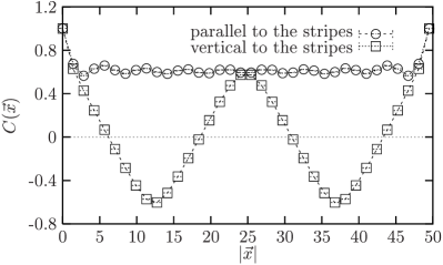
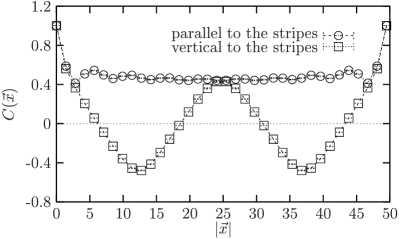
In the case of diagonal stripes we obtain a clear oscillation of the correlation function vertical to the stripes as shown in Figure 5.12. Parallel to the stripes is strongly correlated. Note that here the oscillations do not indicate more than two stripes.
5.3.2 Dispersion relation
In Section 2.4 we discussed the broken Lorentz symmetry and the corresponding deformation of the dispersion relation in non–commutative theory, in the framework of perturbation theory.
In a Lorentz invariant theory the energy squared is linear in and the dispersion relation is given by
| (5.15) |
where is the effective mass. In the non–commutative case equation (5.6) implies a dispersion relation of the form
| (5.16) |
where the last term is the leading one loop IR divergence.
Here we study the dispersion relation non–perturbatively. Since we do not consider renormalization aspects in this model, we are only interested in the momentum dependence of the energy. To this end we considered the two–point correlation function in time direction
| (5.17) |
where is again the spatial Fourier transform that we already used in the definition of the order parameter (5.8). On an infinite lattice decays exponentially in . Since we are on a finite lattice with periodic boundary conditions , the correlator behaves like a cosh function,
| (5.18) |
Here is the energy, where we rescaled the integer representation of the momenta to their physical value
| (5.19) |
The correlator allows us to determine the momentum dependence of the energy, i.e. the dispersion relation, by studying its exponential decay. This can be done either by fitting to the function (5.18) or by studying the ratio of two subsequent values .
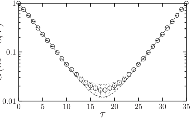
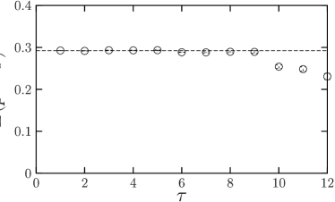
With the first method we obtain as a result of the fit, with
the second method the energy is determined by a plateau. Results are
shown in Figure 5.13. In this example the
system is in the disordered phase and we computed
. These measurements allow us to study the
dispersion relation.
We evaluated configurations close to the disordered – uniform transition and close to disordered – stripe transition. On all configurations we measured with the methods described above, for various momenta . Two example results at are displayed in Figure 5.14. On the left is linear in as one expects in a Lorentz invariant theory. The solid line in this plot is the result of a fit to the dispersion relation (5.15), where we used the effective mass as the only free parameter. Since we are on a finite lattice we see at larger momenta a deviation. Here the momentum dependence of the energy is (if Lorentz symmetry holds). A fit to this function is represented by the dashed line in Figure 5.14. This line fits the data very well. Since the energy minimum is at at this value of , we end up in the uniform phase when we decrease .
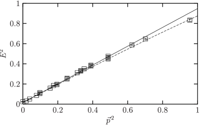
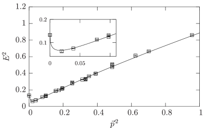
The situation is different for larger . This is shown in Figure 5.14 on the right. In the vicinity of we see here a clear deviation from the dispersion relation (5.15), at large momenta the linear behavior is restored. The increased energy at zero momentum is in full agreement with the perturbatively predicted IR divergence. Due to the discrete compactification (see Section 3.1) a finite lattice spacing serves also as an IR cut–off, along with the finite volume. Therefore we do not see a divergence. Since the cut–off influences the IR behavior we included an ad hoc cut–off , as a consequence of equation (2.38). We fitted the data to the function
| (5.20) |
It turned out that the leading IR divergence in equation (5.16) does not describe the low momentum behavior sufficiently well. Therefore we added a linear term 777Adding more terms in the expansion does not change the results within the errors. in from the expansion of the exponential function in equation (5.6). The relative errors of the fit parameters are shown in Table 5.1. The errors of the parameters of the deformation are rather large, which is not surprising since we have only one data point displaying this effect.
However, the minimum of the energy is here clearly at the smallest non–vanishing momentum. This minimum implies that for decreased the system will be in the striped phase and the vacuum pattern will have two stripes parallel to one of the axes. For the energy increases again, which may indicate the IR divergence (at ).
Here we observe that at small , and equivalently for small
, the effects of UV/IR mixing are strongly suppressed and we
restore the behavior of the commutative theory, including an Ising
type phase transition. At larger the UV/IR mixing effects
become dominant and the phase transition changes its nature. This is
in qualitatively agreement with
the conjecture by Gubser and Sondhi [27].
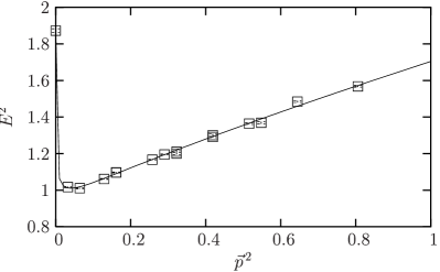
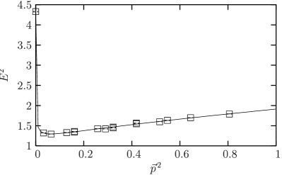
For further increased one expects the minimum at larger
momenta. In addition should increase with . Since at
a slightly larger coupling the expected effect did not show up, we
increased coupling drastically from (the largest value
at that is plotted in the phase diagram
5.2) to and . The results
are shown in Figure 5.15. We clearly see in these
plots that increases with . We fitted the data again
to the fit function (5.20). The results are
the solid lines in Figures 5.15 and 5.16
and the relative errors of the fit parameters are shown in Table
5.1 in the last two lines. At these values of
also the errors of the parameters describing the deformation
of the dispersion relation are under control. The results of the fits
are consistent with the one loop result of perturbation theory
(5.16) over a wide range of .
This is an unexpected result, since at these values of
effects from higher order perturbation theory are expected. One might
conclude here that there are no qualitatively new IR singularities
from higher loop contributions. However, this needs confirmation on
larger lattices.
To identify the minimum of the energy we plotted the dispersion relation in a smaller range (Figure 5.16). On the left, at , the values of the energy at and
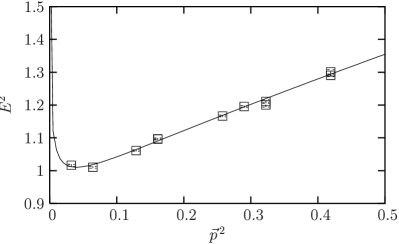
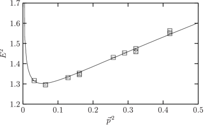
are equal within the statistical errors. From our data it is not possible to predict which of these momentum modes will condense for decreased . On the right in Figure 5.16, at , the minimum of the energy is clearly at the second smallest non–vanishing momentum, which corresponds to . Therefore the pattern in the non–uniform phase will have two diagonal stripes.
5.4 The phase diagram revisited
As we have seen in Subsection 5.3.2, the investigation of the dispersion relation in the disordered phase provides information about the ordered regime. The mode that drives the phase transition, and therefore indicates the pattern of the ordered regime, is given by the momentum that minimizes the energy.
This might give more insight into the transition region between uniform and striped phase. The difference between the energy at and at indicates the type of ordering that will occur in the ordered regime. In the uniform phase this difference is negative and in the striped phase positive. Equal energies indicate the phase transition.
Since this is a small effect we performed high statistic 888To extract this information we used configurations. simulations at in the range of , which is marked as transition region in Figure 5.2. On these configurations we measured the energy gap .
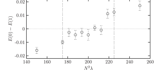
The result is plotted in Figure 5.17, where the
region between vertical lines represent the aforementioned transition
region. Outside this region and at its boundaries we clearly identify
the uniform phase (left) and the striped phase (right). Inside the
region the energy gap is zero within the errors with one exception
close to the striped phase. With this method we cannot identify a
transition line either. However, these measurements clarify why here
the pattern depends on the starting configurations. If and
are almost equal it is (numerically) not clear which mode
drives the phase transitions. Since numerical studies always suffer
from the finite accuracy of computer numbers, it is hardly possible to
resolve these small effects. Therefore already for two slightly
different configurations the system might end up in one case in the
uniform phase and in the other case in the striped phase,
both of which appear to be stable.
Regions where the minimum of the energy is difficult the identify are of course not restricted to the case discussed here. This occurs whenever the difference between the minimum of the energy and the next larger value of the energy is small compared to the absolute value of the energies. This is certainly the case when the minimum of the energy is changing with respect to the momentum. This obviously takes place in Figure 5.16 on the left. We also see this behavior at large as Figure 5.16 on the right shows. In the first case we face the same problem as in the uniform – non–uniform transition area, which does not allow us to determine the behavior in the ordered regime.
In the latter case the two lowest values of the energy are too close to resolve the correct pattern in the striped phase with our algorithm. However, from the analysis of the dispersion relation in the disordered phase we know that at and the striped phase has –patterns. The additional –patterns in Figure 5.8 are only meta–stable.
It is evident that more complex pattern will occur at further
increased . However, in the limit of strong coupling the
kinetic term in the action (5.2) becomes irrelevant.
In Monte Carlo studies this causes a dramatic increase of the
simulations steps that are needed to achieve the equilibrium (see
Appendix A).
Finally we comment on the orders of the phase transitions. We did not study this topic systematically, but we have some indications of which orders the transitions could be.
The phase transition between disordered and ordered phase seems to be most likely of second order. We assume that because we do not see any indication of hysteresis at this transition. This holds for both, the disordered – uniform and the disordered – non–uniform transition. To study the hysteresis we performed simulations starting from the disordered phase and by slowly decreasing we entered the ordered regime. Once the system was clearly in the ordered regime we increased slowly towards the disordered phase. On these configurations we measured the order parameter. In a first order phase transition the order parameter would be different on both way. Since this hysteresis did not show up we assume a second order phase transition.
We did not found a convincing indication of the order of the transition from the uniform to the striped phase. Here we obtained a transition region which prevents a prediction of the order.
Chapter 6 The 2d non–commutative scalar model
The occurrence of stripes in the ground state implies the spontaneous
breakdown of translation invariance. The case is particularly
interesting in this respect. Gubser and Sondhi argued based on an
action of the Brazovskiian form [28] and the
Mermin–Wagner theorem
[29, 30, 31] that stripes cannot
be stable in . However, Ambjørn
and Catterall pointed out that this theorem
is not applicable, because here we deal with a non–local action as
the star–product shows. In fact they did observe non–uniform
patterns in their numerical results for non–commutative
model in [88], where the two
coordinates obey the commutator relation (2.18). In
general their results agree qualitatively with the results we got in
. The only difference was that they obtained more complicated
patterns than the two–stripe
pattern at rather small coupling .
Inspired by their results we also studied the 2d version of the non–commutative model. In two dimensions the action reads
| (6.1) |
where we used the twist–eaters (3.32) as shift operators . We performed the similar measurements as we did in beginning with the phase diagram. Again we used the order parameter (5.11), but since we are in two dimensions there is no sum over the time .
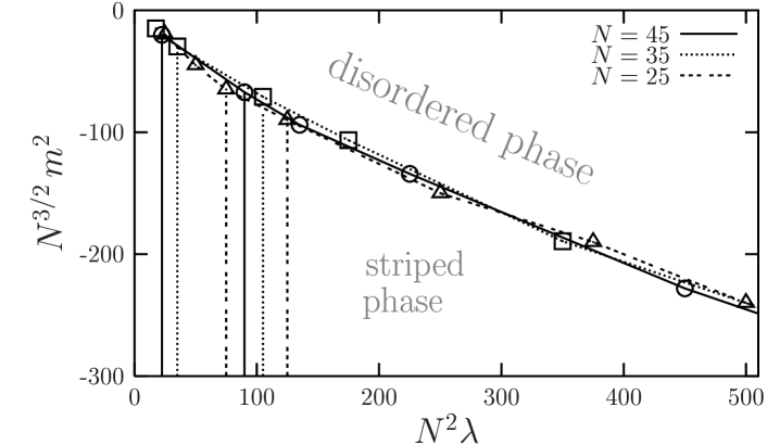
The phase diagram we obtained is plotted in Figure
6.1. As in the 3d case the ordered regime is
split into a uniform and into a striped phase in agreement with
Ambjørn and Catterall. In this case it
takes the factors and on the axes to stabilize the
phase
transitions in .
We also analyzed the striped phase in the range of the parameters that are plotted in Figure 6.1. In this range we always obtained patterns with two stripes. Since Ambjørn and Catterall obtained multi–stripes already at these values of the coupling, we tried to understand the origins of these differences. According to Ref. [88] they used an algorithm that updates the complete matrix at once, in contrast to our algorithm where we updated pairs of matrix elements. Therefore we applied the same algorithm (although it has thermalization and ergodicity problems see Section A.3) and indeed we also discovered other patterns than two stripes. Some example snapshots at are plotted in Figure 6.2. These patterns show up after approximately simulation steps (starting form a random configuration) and survived about further update steps. After increasing the number of update steps further to approximately to steps all patterns turn into the two stripe pattern (Figure 6.2 on the right) independent of the


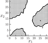
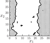
starting configuration.
111In fact we faced the same problem in our study of the 3d model.
In a first attempt we used the same algorithm as in Ref. [88] and we obtained multi stripes already at
. Since we saw a dependence of the patterns on the starting
configuration we improved the algorithm, which unmasked these patterns
as meta–stable.
We show here examples at , but the situation is the same at
. However, the main result in Ref. [88] is of
course the spontaneous breakdown of the translation invariance, and
therefore the existence of a striped phase, which was not expected in
two dimensions. In this point our results fully agree with those of
Ambjørn
and Catterall.
We also computed the spatial correlation function defined in equation (5.14). As in we obtained in the striped phase a strong correlation parallel to the stripes and a strong anti–correlation vertical to the stripes.
For very large coupling we finally obtained stable multi–stripe patterns. One example at is shown in Figure 6.3 on the left.
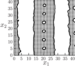
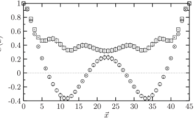
For all starting configurations we arrive at the same pattern, which persists for an apparently unlimited number of update steps even for the improved algorithm (A.13).
The pattern in Figure 6.3 has four stripes where the stripes themselves have some substructure. On the right we plotted the correlation function in position space (5.14). The stripes show up as an oscillation around zero of this correlator perpendicular to the stripes. The substructure of the stripes leads to a slight oscillation of the correlator parallel to the stripes.
Chapter 7 Summary and conclusion
We investigated non–commutative field theories in lower dimensions
non–perturbatively in the lattice approach. Since the non–local
star–product arises also in the lattice formulation it is not
suitable for a direct Monte Carlo investigation. Therefore we used a
finite dimensional representation of the operator formulation
of these field theories. This leads to dimensionally reduced models.
In non–commutative gauge theory the reduced model (reduced to ) is given by the twisted Eguchi Kawai model (TEK). Within this model we investigated the continuum limit of 2d non–commutative theory. In the TEK this limit corresponds to the large double scaling limit. To this end we studied the double scaling limit of the 1–point function and the 2–point function of Wilson loops as well as the 2–point function of Polyakov lines.
The first conclusion from our simulation results is that we do observe a double scaling limit as . This corresponds to the continuum limit of the non–commutative gauge theory, which has therefore also finite observables. This observation demonstrates the non–perturbative renormalizability of 2d non–commutative gauge theory.
The Wilson loop follows an area law at small physical areas, and in this regime non–commutative gauge theory agrees with planar standard gauge theory. However, at larger areas the Wilson loop becomes complex and the real part (the mean values over both loop orientations) begins to oscillate around zero. The phase is proportional to the physical area enclosed by the Wilson loop, irrespectively of its shape, and the coefficient of proportionality is given by the inverse of the non-commutativity parameter . This agrees with the Aharonov–Bohm effect in the presence of a constant magnetic background field
Our results support this law, which is also a key element of the Seiberg and Witten description of non–commutative gauge theory [8]. Moreover, the same law also occurs in condensed matter physics: if one assumes a plane crossed by a constant magnetic flux, then the electrons in this plane can be projected to the lowest Landau level in a non–commutative space, where [12, 13, 14].
The behavior of the Wilson loop at large areas implies that we have found a qualitatively new universality class. At first sight, it may look surprising that the non-commutativity — which introduces a short–ranged non–locality in the action — changes the IR behavior of the gauge theory completely. However, this effect does not appear unnatural in the presence of UV/IR mixing. It is remarkable that this mixing effect does not occur in the perturbative expansion of this model, hence our results for large Wilson loops reveal a purely non–perturbative UV/IR mixing.
For the connected Wilson loop 2–point function, as well as the
2–point function of the Polyakov line, we can confirm the large
scaling. These observables are in agreement with a universal wave
function renormalization, which yields a factor for a
connected 2–point function.
The second model we investigated was the 3d non–commutative theory, with a commutative time coordinate and two non–commutative space directions. Again the lattice model is mapped to a dimensionally reduced model, where here the reduced model is one dimensional.
In this model we explored the phase diagram in the – plane. In the ordered phase (at strongly negative ) we found at small values of a uniform order of the Ising type, as in the commutative case. At larger — which amplifies the non–commutative effects — we observed striped patterns. Up to moderate values of we obtained a pattern of two stripes parallel to the axes for . This corresponds to a minimum of the energy at the smallest non–zero lattice momentum. At very large (compared to the coupling at the uniform – non–uniform phase transition) also other patterns showed up, in agreement with the conjecture of Gubser and Sondhi. However, the continuum limit has to be taken to confirm this agreement. We observed the same behavior in (see Chapter 6). Also there the multiple stripes occurred first at rather large values of . The dominance of stripes implies the spontaneous breaking of translation symmetry, which is also possible in 2d since the action is non–local.
In the ordered regime, the spatial correlations are dictated by the dominant pattern: uniform as in the commutative case, or striped with strong correlations in the direction of the stripes and strong anti–correlation vertical to them. This agrees with the prediction in Ref. [27]. In the disordered phase the spatial correlators deviate at small from the exponential decay. At large the decay is again exponential as was predicted from one loop perturbation theory in Ref. [4].
The correlators in momentum space do decay exponentially in time for all momenta. This property allowed us to study the dispersion relation in the disordered phase: at small the dispersion relation behaves qualitatively like in the commutative case, but at large there appears a jump at as a non–commutative effect. Here we observed the energy minimum at for moderate and at very large the minimum is at . The results agree qualitatively with the results obtained in perturbation theory. Also from non–perturbative studies we observed an IR divergent behavior with the predicted divergence. However, since we obtained rather large fitting errors in the parameters of the IR dominant term this needs further confirmation.
Outlook
In this work we presented results of our first steps in the non–perturbative study of non–commutative field theory. The next steps can be divided into next, near future and future projects.
The next project is to study the 3d model at larger values of . We expect from these studies more insight into the stripe structure in the ordered regime as well as into the IR behavior of the theory. Since the smallest non–zero momentum is given by , a study at larger will resolve the interesting low momentum regime better. In addition we want to study the continuum limit and the related question of renormalizability.
The near future project is to study non–commutative field theory in larger dimensions, for example 4d model or 3d gauge theory. Also a two or three dimensional model would be interesting to study. In addition there are plans to study models including fermions for example a non–commutative Gross–Neveu model.
In the long run we want to study models, which allow phenomenological predictions, like non–commutative pure gauge theory or non–commutative QED in .
Acknowledgements: First of all I would like to thank M. Müller–Preußker, D. Lüst and W. Bietenholz for their support and for the pleasurable and inspiring atmosphere, they provided.
In particular I also thank J. Nishimura, who suggested the numerical study of non–commutative field theory. Together with W. Bietenholz we build this small collaboration and I want to thank both for letting me participate in this challenging field of research.
In addition I thank V. Linke. I was a member also of his group and therefore I had the advantages of two working groups. I am indebted to both groups and especially to A. Barresi for helpful discussions about critical phenomena and phase transitions. I also thank S. Shcheredin, A. Sternbeck and C. Urbach for inspiring discussions.
Appendix A The numerical methods
In this appendix we discuss the details of the algorithms we used to simulate the non–commutative models. We start with some general comments on Monte Carlo simulations.
A.1 Monte Carlo simulations
The idea of Monte Carlo (MC) simulations is to integrate approximately the infinite dimensional path integrals that appear in lattice formulation of any Euclidean field theory, with statistical methods.
Vacuum expectation values of some observables are computed in the path integral approach by
| (A.1) |
where is the action. The action may also depend on matter fields, 111In that case also the matter fields have to be integrated. but for simplicity we restrict ourselves to gauge fields . is the partition function
| (A.2) |
A set of gauge fields , one for each link on the lattice, is a called a configuration. The idea of MC simulations is to generate as many configurations as possible via importance sampling. Importance sampling means that the configurations are generated according to the probability
| (A.3) |
In addition to importance sampling a simulation algorithm has to fulfill the condition of ergodicity. This means that for any two configurations and the probability for a transition from one configuration out of the other, within finite number of update steps, is non–zero.
On each configuration the observable is calculated and the result is the value . The expectation value (A.1) is then given by
| (A.4) |
In practice the number of configurations is of course limited and therefore we get an approximation of the expectation value
| (A.5) |
with an associated statistical uncertainty. If the configurations are statistically independent this uncertainty reads
| (A.6) |
where is the average of . In practical applications the configurations generated with a Monte Carlo simulation are always correlated and the error calculated with equation (A.6) is usually underestimated. This correlation in a sequence of configurations is called autocorrelation. For an infinitely large set of configurations the autocorrelation time is defined as
| (A.7) |
There are several methods to take the autocorrelation time into account or to eliminate the effects of autocorrelation. Here we discuss only the methods that were used in this work.
Error estimation
In our evaluation of the sets of observables we used two types of error estimations: the binning method and the jack–knife method. Both methods are based on dividing the set of observables into a number of subsets. In each subset the average is calculated according to equation (A.5), where the number of configurations has to be replaced by the number of configurations in a subset. The result is a set of averages .
Within the binning method one considers the averages as statistically independent and therefore the error is given by equation (A.6), where now the set of averages is used. The error calculated in this way varies with the number of bins . In order not to underestimate the statistical error one should compute the errors for different values of and take the largest error.
The jack–knife method uses the averages to construct statistically independent subsets in the following way,
| (A.8) |
Here is the average of the omitting the subset . The error is now calculated according to equation (A.6), using as subset. This method has the advantage that it allows to compute the error of quantities that consist of two or more expectation values like the connected part of 2–point functions.
Steps of a Monte Carlo simulation
Before starting a simulation one has to perform tests of the
algorithm. This is of course always important. Here it is
indispensable, since in the case discussed there are no results
available in the literature to compare qualitatively the obtained
results. The test for each algorithm will be discussed at the end of
the corresponding Section. After these tests the simulations can be
started. Here we briefly
summarize the main steps of a typical Monte Carlo simulation.
A Monte Carlo simulation consist of
-
1.
choosing a starting configuration. This can be either a random configuration or the gauge field set to certain values.
-
2.
performing update steps I: the first configurations are in general not distributed according to (A.3), since a random configurations is located anywhere in configuration space. Therefore one performs update steps till the system is in equilibrium. These steps are called thermalization steps.
-
3.
performing update steps II: having reached the equilibrium a set of configurations is evaluated using equation (A.5). The evaluated configurations should be separated by the autocorrelation time.
A.2 Details of the TEK Model simulation
For the TEK model we chose the heat bath algorithm [89]. In this method each link variable is updated separately, while the others are fixed. A new link is suggested and it is accepted with the probability
| (A.9) |
where is the part of the action that depends on . In other words, it is the sum over all plaquettes which involved , times the coupling . To enable this disentanglement the action has to be linear in the link variables.
In the form of equation (4.6), the action cannot be simulated with the heat bath algorithm because it is not linear in the matrices . Following Ref. [90] we introduce an auxiliary field , which enters in a Gaussian form and linearizes the action in ,
| (A.10) |
The auxiliary field consists of general complex matrices, and their integration reproduces the TEK action (4.6), if . The matrices are updated in subgroups in the spirit of Cabbibo and Marinari [91], and the update of is done by generating Gaussian variables.
With this algorithm we generated configurations at various values of keeping fixed. Table A.1 shows the number of configurations we generated at each value of .
| 25 | 35 | 55 | 85 | 125 | 195 | 255 | 515 | |
|---|---|---|---|---|---|---|---|---|
| # of configurations | 9000 | 8400 | 20000 | 8000 | 3400 | 260 | 120 | 18 |
All configurations are separated by update steps, which is more than the autocorrelation time in these simulations (the maximum autocorrelation time measured was update steps). We started the simulations with random configurations and it took approximately update steps to reach equilibrium.
The errors of the Wilson loops (4.18) and the
Polyakov lines (4.22) were computed with the binning
method. To estimate the errors of the two–point functions of Wilson
loops (4.20) we used the jack–knife
method, since this quantity consists of two expectation values.
The simulations were performed on Intel PCs with the operating system Linux. The PCs had a clock rate of MHz. The generation of the configurations took approximately five month.
For the measurement of the observables we had to compute high powers of matrices. Since they are not sparse matrices, in contrast to typical situations in lattice gauge theory, there is no simplified method to calculate these powers. One way to compute these powers is to evaluate the eigenvalues of the matrices first. All powers of the matrix are then just powers of the eigenvalues values. In this case one can use for example the conjugate gradient algorithm, which yields the eigenvalues up to a required precision. Unfortunately with this method we needed more matrix multiplications for a reasonable precision than with the direct multiplication.
Therefore we decided the use a slightly modified direct multiplication of the matrices. The aim of the modification was to use more than one computer to calculate the powers of a given matrix without wasting too much computer time. 222Note that we were not computing on a parallel machine. Assume that we want to compute . To accelerate the calculation we want to use five computers, where to first computes to the second to and so on. This is of course only faster than using one computer if we manage to calculate the starting power for each computer in a fast way.
For this we write the starting exponent in binary form. For example for the exponent 60
| (A.11) |
In the next step these different powers of are computed by taking repeatedly the square of the matrix. In the above example these are 5 matrix multiplications. The final result we get by multiplying the powers which have a non–vanishing coefficient, here multiplications, which means that we computed with matrix multiplications.
After the starting power of is generated the following powers are computed via direct multiplication. With this method it took approximately two months to evaluate the configurations in Table A.1.
Tests of the algorithm
In this model there exists a very stringent test of the implementation of the algorithm, namely the planar limit discussed in Section 4.1.3. In this limit there is an exact solution in the large limit [81]. We reproduced these results in the planar limit with our code, confirming the validity of our investigations. In fact the program we used was only slightly modified compared to Ref. [84]. There the planar limit of the TEK model was studied, though, with a different twist and with even , also reproducing the analytic solution of the planar limit.
A.3 Details of the model simulation
For the scalar model we chose the standard Metropolis algorithm [92]. The idea of this algorithm is to suggest a new configuration, and accept this configuration with the probability
| (A.12) |
If the action of the new configuration is smaller than the action of the old configuration it is accepted in any case, vice versa the new configuration is accepted with the probability . The explicit update was performed by choosing an element of the Hermitian matrices according to
| (A.13) |
Here is a random complex number with and is an overall scale of the suggested changes, which has to be fixed. For every pair of complex conjugated elements we perform the accept–reject step (A.12).
The parameter should be chosen in a way to get a reasonable acceptance rate. If the acceptance rate is close to 1, the generated configurations are strongly correlated. If it is close to zero hardly any configurations are generated. A reasonable value would be , so one might try to fix to a value providing this acceptance rate.
However, in this study we explore a phase diagram and the optimal value of might depend on the different phases or it changes close to the phase transition. Therefore we decided to implement a dynamical value : after updating the complete lattice we measure the acceptance rate. If the acceptance rate is above we increase by , if the acceptance rate is below we decrease by . 333Note that oscillations between two values of are excluded with this choice.
We choose the real and the imaginary part of from the interval
times . A reasonable starting value of
is then . In most cases
stabilized after update steps, depending on the
coupling , at a value close to the starting value. However,
at very large values of the coupling stabilized at a
rather small value one order
of magnitude smaller than , see below.
The update of every independent matrix element of is of course more expensive than updating each matrix at once. However, it improves thermalization as well as ergodicity properties. In Figure A.1 we show the history of the action for three different starting configurations.
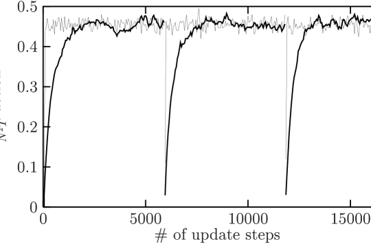
For the history shown by the thin line we used the update procedure (A.13) and the thick lines represent the result when we update each matrix at once. In both methods we used a dynamical parameter . First of all we see that the system thermalize much faster when updating the elements separately. This already compensates the additional computer time needed for this algorithm. We also see that with the procedure, where we update one matrix at once, the action fluctuates much less than with the update procedure (A.13). This means that we hardly proceed in configuration space and the configurations are strongly correlated.
The reason for this is that if we change a complete matrix the change of the action is rather large and we get a reasonable acceptance rate only if we decrease the overall factor to a tiny value. The configuration is hardly changed within an update step.
In practice we also measured as an technical parameter.
It depends only slightly on , but it strongly depends on the
coupling . For very large couplings we have again an
ergodicity problem. The values of discussed in Chapter
5 can be considered as the upper limit for the
algorithm described here.
Besides the qualitative structure of the phase diagram, no details about the phases structure of this theory were known. As we expect a striped phase, with general patterns, we are possibly dealing in this phase with meta–stable states, which are usually difficult to identify.
Therefore we always started from six independent (random) starting configurations and initialized the random number generator differently, i. e. we made for any set of six independent simulations. This is of course much more expensive than starting only from one configuration, because we have to thermalize all six runs. It has several benefits, however. If there are meta–stable states, they certainly depend on the starting conditions. With different starting conditions we should therefore see, in that case, different vacua. This could indicate that we should apply more thermalization steps. On the other hand, if we thermalize the system further, this shows that the algorithm is not ergodic, and we are stuck in a subset of configuration space.
In fact, we saw these different meta–stable states, indicated by different patterns, at some stage of the simulations. At moderate values of , applying more thermalization steps all starting conditions lead to the same results. At very large this tunneling from meta–stable patterns to the stable pattern occurred only close to the ordered – disordered phase transition (see Section 5.4).
A second advantage is that it clarifies the error estimation. As
discussed in the last Section, the number of bins influences the
statistical error in the binning as well as in the jack–knife method.
In our case there is a natural choice of bins. Since we generate six
statistically independent sets of configurations, we also chose six
bins for the error analysis.
Table A.2 shows the number of configurations we generated with the algorithm described above. The necessary statistics to study the phase diagram is relatively small; this is shown in the second row of table A.2.
| 15 | 25 | 35 | 45 | ||
|---|---|---|---|---|---|
| # of configurations | phase diagram | 300 | 180 | 60 | 30 |
| 2–point functions | 10000 | 10000 | 5000 | 3000 |
To compute the 2–point functions, especially those in momentum space, we needed significantly more configurations to obtain small statistical errors. At some values of the parameters we performed high statistic simulations where we doubled the number of configurations. The autocorrelation time in this simulation was in the range – update steps, depending on the observable and on the point in the phase diagram under consideration. Therefore we measured the observables from configurations separated by update steps.
It took approximately 10 month on PCs (with a clock rate in the range – MHz) to generate the configurations in Table A.2. The evaluation of the configuration did not increase the overall needed computer time, since we did not need high powers of the matrices . Most of the (usually expensive) matrix multiplications are in this evaluation multiplications with the constant twist eaters (see Chapter 5). These multiplication can be performed by shifting or modifying the phases of matrix elements of , which is much faster than a direct multiplication.
Tests of the algorithm
To test the algorithm is here more sophisticated than in the TEK model, since no exact solution is known in this case. Therefore we computed the expectation value of the action in equation (5.2) to the first order in ,
| (A.14) |
For small our algorithm should reproduce this result. We give now a brief account on how the coefficients and were obtained [93].
To compute we used the fact that the partition function is invariant under a change of variables . The integration measure and the action transform under this shift like
| (A.15) |
where the transformation of the action is only valid in first order in . Since the partition function is invariant under this transformation we obtain
| (A.16) |
To satisfy this equation the term in square brackets has to vanish. This amounts to the condition
| (A.17) |
Note that the result for is independent of and .
For the determination of we extend the above consideration to the interacting case . This leads to the identity
| (A.18) |
Therefore is given by
| (A.19) |
This expectation value can be calculated by transforming the partition
function into momentum space, with the discrete Fourier transformation
defined in equation (3.38) and using Wick’s theorem to
evaluate the resulting expectation value. The equation for the
coefficient is now given by a sum over momenta. The term that is
summed over is very lengthy and complex, therefore we will not show
the explicit result. However, for given parameters and it
can be computed for example with the program mathematica.
To test if our algorithm provides this result, we computed the action at and . The coefficient is always given by . For the chosen value of we find . Figure A.2 clearly confirms that our program reproduces this result.
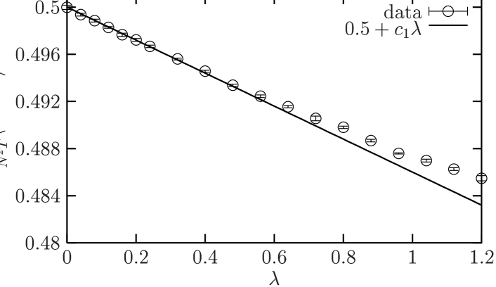
References
- [1] H. S. Snyder. Quantized Space–time. Phys. Rev. 71, 38 (1947).
- [2] C. N. Yang. On Quantized Space–time. Phys. Rev. 72, 874 (1947).
- [3] T. Filk. Divergencies in a Field Theory on Quantum Space. Phys. Lett. B376, 53 (1996).
- [4] S. Minwalla, M. Van Raamsdonk, and N. Seiberg. Non–commutative Perturbative Dynamics. JHEP 02, 020 (2000), hep-th/9912072.
- [5] J. C. Varilly and J. M. Gracia-Bondia. On the Ultraviolet Behaviour of Quantum Fields over Non–commutative Manifolds. Int. J. Mod. Phys. A14, 1305 (1999), hep-th/9804001.
- [6] A. Connes and M. Rieffel. Yang–Mills for Non–commutative Two–tori. Contemp. Math. Oper. Algebra. Math. Phys. 62, 237 (1987).
- [7] A. Abouelsaood, C. Callan, C. R. Nappi, and S. A. Yost. Open Strings in Background Gauge Fields. Nucl. Phys. B280, 599 (1987).
- [8] N. Seiberg and E. Witten. String Theory and Non–commutative Geometry. JHEP 09, 032 (1999), hep-th/9908142.
- [9] S. Doplicher, K. Fredenhagen, and J. E. Roberts. Space–time Quantization Induced by Classical Gravity. Phys. Lett. B331, 39 (1994).
- [10] S. Doplicher, K. Fredenhagen, and J. E. Roberts. The Quantum Structure of Space–time at the Planck Scale and Quantum Fields. Commun. Math. Phys. 172, 187 (1995).
- [11] M. R. Douglas and N. A. Nekrasov. Non–commutative Field Theory. Rev. Mod. Phys. 73, 977 (2002), hep-th/0106048.
- [12] S. M. Girvin and A. H. MacDonald. Off Diagonal Long Range Order, Oblique Confinement, and the Fractional Quantum Hall Effect. Phys. Rev. Lett. 58, 1252 (1987).
- [13] J. Bellissard, A. van Elst, and H. Schulz-Baldes. The Non–commutative Geometry of the Quantum Hall Effect. (1994), cond-mat/9411052.
- [14] S. M. Girvin. The Quantum Hall Effect: novel Excitations and broken Symmetries. (1998), cond-mat/9907002.
- [15] L. Susskind. The Quantum Hall Fluid and Non–commutative Chern Simons Theory. (2001), hep-th/0101029.
- [16] A. P. Polychronakos. Quantum Hall States on the Cylinder as Unitary Matrix Chern–Simons Theory. JHEP 06, 070 (2001), hep-th/0106011.
- [17] W. Bietenholz, F. Hofheinz, and J. Nishimura. The Renormalizability of 2d Yang–Mills Theory on a Non–commutative Geometry. JHEP 09, 009 (2002), hep-th/0203151.
- [18] W. Bietenholz, F. Hofheinz, and J. Nishimura. Simulating Non–commutative Field Theory. Nucl. Phys. Proc. Suppl. 119, 941 (2003), hep-lat/0209021.
- [19] W. Bietenholz, F. Hofheinz, and J. Nishimura. Non–commutative Field Theories beyond Perturbation Theory. Fortsch. Phys. 51, 745 (2003), hep-th/0212258.
- [20] K. Osterwalder and R. Schrader. Axioms for Euclidean Green’s Functions. 2. Commun. Math. Phys. 42, 281 (1975).
- [21] D. Bahns, S. Doplicher, K. Fredenhagen, and G. Piacitelli. On the Unitarity Problem in Space–time Non–commutative Theories. Phys. Lett. B533, 178 (2002), hep-th/0201222.
- [22] C. Rim and J. Yee. Unitarity in Space–time Non–commutative Field Theories. (2002), hep-th/0205193.
- [23] Y. Liao and K. Sibold. Time–ordered Perturbation Theory on Non–commutative Space–time. II. Unitarity. Eur. Phys. J. C25, 479 (2002), hep-th/0206011.
- [24] A. Connes, M. R. Douglas, and A. Schwarz. Non–commutative Geometry and Matrix Theory: Compactification on Tori. JHEP 02, 003 (1998), hep-th/9711162.
- [25] J. Ambjørn, Y. M. Makeenko, J. Nishimura, and R. J. Szabo. Lattice Gauge Fields and Discrete Non–commutative Yang–Mills Theory. JHEP 05, 023 (2000), hep-th/0004147.
- [26] R. J. Szabo. Quantum Field Theory on Non–commutative Spaces. (2001), hep-th/0109162.
- [27] S. S. Gubser and S. L. Sondhi. Phase Structure of Non–commutative Scalar Field Theories. Nucl. Phys. B605, 395 (2001), hep-th/0006119.
- [28] S. Brazovkii. Phase Structure of an Isotropic System to a Non–uniform State. Zh. Eksp. Teor. Fiz A 15, 319 (1975).
- [29] N. D. Mermin and H. Wagner. Absence of Ferromagnetism or Antiferromagnetism in One–dimensional or Two–dimensional Isotropic Heisenberg Models. Phys. Rev. Lett. 17, 1133 (1966).
- [30] P. C. Hohenberg. Existence of Long–Range Order in One and Two Dimensions. Phys. Rev. 158, 383 (1967).
- [31] S. R. Coleman. There are no Goldstone Bosons in Two Dimensions. Commun. Math. Phys. 31, 259 (1973).
- [32] G. Chen and Y. Wu. Renormalization Group Equations and the Lifshitz Point in Non–commutative Landau–Ginsburg Theory. Nucl. Phys. B622, 189 (2002), hep-th/0110134.
- [33] K. Matsubara. Restrictions on Gauge Groups in Non–commutative Gauge Theory. Phys. Lett. B482, 417 (2000), hep-th/0003294.
- [34] A. Armoni. Comments on Perturbative Dynamics of Non–commutative Yang–Mills Theory. Nucl. Phys. B593, 229 (2001), hep-th/0005208.
- [35] M. Hayakawa. Perturbative Analysis on Infrared Aspects of Non–commutative QED on R**4. Phys. Lett. B478, 394 (2000), hep-th/9912094.
- [36] B. Jurco, S. Schraml, P. Schupp, and J. Wess. Enveloping Algebra Valued Gauge Transformations for Non–Abelian Gauge Groups on Non–commutative Spaces. Eur. Phys. J. C17, 521 (2000), hep-th/0006246.
- [37] C. Chu and H. Dorn. Non–commutative SU(N) and Gauge Invariant Baryon Operator. Phys. Lett. B524, 389 (2002), hep-th/0110147.
- [38] I. Chepelev and R. Roiban. Renormalization of Quantum Field Theories on Non–commutative R**d. I: Scalars. JHEP 05, 037 (2000), hep-th/9911098.
- [39] S. Sarkar. On the UV Renormalizability of Non–commutative Field theories. JHEP 06, 003 (2002), hep-th/0202171.
- [40] L. Griguolo and M. Pietroni. Wilsonian Renormalization Group and the Non–commutative IR/UV Connection. JHEP 05, 032 (2001), hep-th/0104217.
- [41] L. Griguolo and M. Pietroni. Hard Non–commutative Loops Resummation. Phys. Rev. Lett. 88, 071601 (2002), hep-th/0102070.
- [42] H. O. Girotti, M. Gomes, V. O. Rivelles, and A. J. da Silva. A Consistent Non–commutative Field Theory: The Wess–Zumino Model. Nucl. Phys. B587, 299 (2000), hep-th/0005272.
- [43] H. O. Girotti, M. Gomes, A. Yu. Petrov, V. O. Rivelles, and A. J. da Silva. The Three–Dimensional Non–commutative Nonlinear Sigma Model in Superspace. Phys. Lett. B521, 119 (2001), hep-th/0109222.
- [44] R. Wulkenhaar. Non–renormalizability of –expanded Non–commutative QED. JHEP 03, 024 (2002), hep-th/0112248.
- [45] D. Colladay and V. A. Kostelecky. Lorentz-violating Extension of the Standard Model. Phys. Rev. D58, 116002 (1998), hep-ph/9809521.
- [46] S. M. Carroll, J. A. Harvey, V. A. Kostelecky, C. D. Lane, and T. Okamoto. Non–commutative Field Theory and Lorentz Violation. Phys. Rev. Lett. 87, 141601 (2001), hep-th/0105082.
- [47] G. Amelino-Camelia, L. Doplicher, S. Nam, and Y. Seo. Phenomenology of particle production and propagation in string-motivated canonical noncommutative spacetime. (2001), hep-th/0109191.
- [48] A. Matusis, L. Susskind, and N. Toumbas. The IR/UV Connection in the Non–commutative Gauge Theories. JHEP 12, 002 (2000), hep-th/0002075.
- [49] G. Amelino-Camelia, J. Ellis, N. E. Mavromatos, D. V. Nanopoulos, and Subir Sarkar. Potential Sensitivity of Gamma-Ray Burster Observations to Wave Dispersion in Vacuo. Nature 393, 763 (1998), astro-ph/9712103.
- [50] S. D. Biller et al. Limits to Quantum Gravity Effects from Observations of TeV Flares in Active Galaxies. Phys. Rev. Lett. 83, 2108 (1999), gr-qc/9810044.
- [51] The HESS Project. http://www.mpi-hd.mpg.de/hfm/HESS/HESS.html.
- [52] T. Lohse, 02 2003. Private Communication.
- [53] A. de Angelis. GLAST, the gamma-ray large area space telescope. (2000), astro-ph/0009271.
- [54] F. Aharonian et al. TeV Gamma Rays from the Blazar H 1426+428 and the diffuse Extragalactic Background Radiation. (2002), astro-ph/0202072.
- [55] K. Greisen. End to the Cosmic Ray Spectrum? Phys. Rev. Lett. 16, 748 (1966).
- [56] F. W. Stecker and O. C. De Jager. New Upper Limits on Intergalactic Infrared Radiation from High–energy Astrophysics. Astrophys. J. 415, L71 (1993).
- [57] G. Zatsepin and V. Kuzmin. Upper Limit of the Spectrum of Cosmic Rays. JETP Lett. 4, 78 (1966).
- [58] N. Hayashida et al. Updated AGASA event list above 4*10**19-eV. Astrophys. J. 522, 225 (1999), astro-ph/0008102.
- [59] G. Amelino-Camelia and T. Piran. Planck-scale deformation of Lorentz symmetry as a solution to the UHECR and the TeV-gamma paradoxes. Phys. Rev. D64, 036005 (2001), astro-ph/0008107.
- [60] J. L. Hewett, F. J. Petriello, and T. G. Rizzo. Signals for Non–commutative Interactions at Linear Colliders. Phys. Rev. D64, 075012 (2001), hep-ph/0010354.
- [61] M. M. Sheikh-Jabbari. Renormalizability of the Supersymmetric Yang–Mills Theories on the Non–commutative Torus. JHEP 06, 015 (1999), hep-th/9903107.
- [62] T. Krajewski and R. Wulkenhaar. Perturbative Quantum Gauge Fields on the Non–commutative Torus. Int. J. Mod. Phys. A15, 1011 (2000), hep-th/9903187.
- [63] I. Ya. Aref’eva, D. M. Belov, A. S. Koshelev, and O. A. Rytchkov. UV/IR Mixing for Non–commutative Complex Scalar Field Theory. II: Interaction with Gauge Fields. Nucl. Phys. Proc. Suppl. 102, 11 (2001), hep-th/0003176.
- [64] J. A. Aguilar-Saavedra et al. TESLA Technical Design Report Part III: Physics at an e+e- Linear Collider. (2001), hep-ph/0106315.
- [65] T. Abe et al. Linear Collider Physics Resource Book for Snowmass 2001. 4: Theoretical, Accelerator, and Experimental Options. (2001), hep-ex/0106058.
- [66] R. W. Assmann et al. A 3-TeV e+ e- Linear Collider Based on CLIC Technology. SLAC-REPRINT-2000-096.
- [67] S. Godfrey and M. A. Doncheski. Signals for Non–commutative QED in and Collisions. Phys. Rev. D65, 015005 (2002), hep-ph/0108268.
- [68] T. G. Rizzo. Signals for Non–commutative QED at Future e+ e- Colliders. (2002), hep-ph/0203240.
- [69] I. Hinchliffe and N. Kersting. Review of the Phenomenology of Non–commutative Geometry. (2002), hep-ph/0205040.
- [70] A. Anisimov, T. Banks, M. Dine, and M. Graesser. Comments on Non–commutative Phenomenology. Phys. Rev. D65, 085032 (2002), hep-ph/0106356.
- [71] S. Godfrey and M. A. Doncheski. Phenomenology of Non–commutative Field Theories. (2002), hep-ph/0211247.
- [72] K. G. Wilson. Confinement of Quarks. Phys. Rev. D10, 2445 (1974).
- [73] J. Ambjørn, Y. M. Makeenko, J. Nishimura, and R. J. Szabo. Finite N Matrix Models of Non–commutative Gauge Theory. JHEP 11, 029 (1999), hep-th/9911041.
- [74] J. Ambjørn, Y. M. Makeenko, J. Nishimura, and R. J. Szabo. Non–perturbative Dynamics of Non–commutative Gauge Theory. Phys. Lett. B480, 399 (2000), hep-th/0002158.
- [75] R. J. Szabo. Discrete Non–commutative gauge theory. Mod. Phys. Lett. A16, 367 (2001), hep-th/0101216.
- [76] P. van Baal and B. van Geemen. A Simple Construction of Twist Eating Solutions. J. Math. Phys. 27, 455 (1986).
- [77] T. Eguchi and H. Kawai. Reduction of Dynamical Degrees of Freedom in the Large N Gauge Theory. Phys. Rev. Lett. 48, 1063 (1982).
- [78] G. Bhanot, U. M. Heller, and H. Neuberger. The Quenched Eguchi–Kawai Model. Phys. Lett. B113, 47 (1982).
- [79] A. González-Arroyo and M. Okawa. A Twisted Model for Large N Lattice Gauge Theory. Phys. Lett. B120, 174 (1983).
- [80] A. González-Arroyo and C. P. Korthals Altes. Reduced Model for Large N Continuum Field Theories. Phys. Lett. B131, 396 (1983).
- [81] D. J. Gross and E. Witten. Possible Third Order Phase Transition in the Large N Lattice Gauge Theory. Phys. Rev. D21, 446 (1980).
- [82] H. Aoki, N. Ishibashi, S. Iso, H. Kawai, Y Kitazawa, and T. Tada. Non–commutative Yang–Mills in IIB Matrix Model. Nucl. Phys. B565, 176 (2000), hep-th/9908141.
- [83] K. Fabricius and O. Haan. Numerical Analysis of the Twisted Eguchi–Kawai Model in Two–Dimensions. Phys. Lett. B131, 399 (1983).
- [84] T. Nakajima and J. Nishimura. Numerical Study of the Double Scaling Limit in Two– dimensional Large N Reduced Model. Nucl. Phys. B528, 355 (1998), hep-th/9802082.
- [85] N. Seiberg, L. Susskind, and N. Toumbas. Space–time Non–commutativity and Causality. JHEP 06, 044 (2000), hep-th/0005015.
- [86] H. Bozkaya, P. Fischer, H. Grosse, M. Pitschmann, V. Putz, M. Schweda, and R. Wulkenhaar. Space–time Non–commutative Field Theories and Causality. (2002), hep-th/0209253.
- [87] J. Gomis and T. Mehen. Space–time Non–commutative Field Theories and Unitarity. Nucl. Phys. B591, 265 (2000), hep-th/0005129.
- [88] J. Ambjørn and S. Catterall. Stripes from (Non–commutative) Stars. Phys. Lett. B549, 253 (2002), hep-lat/0209106.
- [89] M. Creutz. Monte Carlo Study of Quantized SU(2) Gauge Theory. Phys. Rev. D21, 2308 (1980).
- [90] K. Fabricius and O. Haan. Heat Bath Method for the Twisted Eguchi–Kawai Model. Phys. Lett. B143, 459 (1984).
- [91] N. Cabibbo and E. Marinari. A new Method for Updating SU(N) Matrices in Computer Simulations of Gauge Theories. Phys. Lett. B119, 387 (1982).
- [92] G. Bhanot. The Metropolis Algorithm. Rept. Prog. Phys. 51, 429 (1988).
- [93] J. Nishimura, 02 2002. Private Communication.