Transmogrifying Fuzzy Vortices

Abstract:

We show that the construction of vortex solitons of the noncommutative Abelian-Higgs model can be extended to a critically coupled gauged linear sigma model with Fayet-Illiopolous D-terms. Like its commutative counterpart, this fuzzy linear sigma model has a rich spectrum of BPS solutions. We offer an explicit construction of the degree$-k$ static semilocal vortex and study in some detail the infinite coupling limit in which it descends to a degree$-k$ $\mathbb{C}\mathbb{P}^{N}$ instanton. This relation between the fuzzy vortex and noncommutative lump is used to suggest an interpretation of the noncommutative sigma model soliton as tilted D-strings stretched between an NS5-brane and a stack of D3-branes in type IIB superstring theory.

bbold12 bbold8

1 Introduction

A little more than a decade ago, the study of electroweak strings in a modified Abelian-Higgs theory initiated in [35] revealed a curious new vortex solution. As the story goes, vortices are indeed enigmatic objects [34] and the semilocal vortices found in [35] are no exception. Firstly, standard lore holds that a non-simply-connected vacuum manifold is a necessary condition for the existence of stable, finite energy cosmic string solutions. If this is anything to go by, the very existence of these semilocal vortices should be called into question since the vacuum manifold of the modified Abelian-Higgs theory is $S^{3}$. Yet exist they do. Consequently, a more consistent condition was offered in [17]. Semilocal vortices (actually, this holds for other defects as well) form in theories exhibiting spontaneous symmetry breaking and whose vacuum manifold is fibred by the action of the gauge group in some non-trivial way. In this same work it was realised also that the low momentum dynamics of these vortices bear a striking resemblance to the $2-$dimensional lump solutions of the $\mathbb{C}\mathbb{P}^{N}$ nonlinear sigma model. Since then, this similarity between the modified Abelian-Higgs theory (a.k.a gauged linear sigma model) and the $\mathbb{C}\mathbb{P}^{N}$ (or, more generally, Grassmannian) sigma model has found itself the subject of much attention [10, 30, 40]. Nevertheless, much of what is known about the semilocal vortex is only asymptotic. Even its descent to the lump in the infinite coupling limit is only exact at spatial infinity and suffers Skyrme term corrections at smaller radial distances. This is the allure and frustration of vortices; as simple as their defining equations seem, they are also remarkably unyielding.

Until a short time ago, the only avenue toward tractable vortex equations was a curvature deformation of the background space in which the vortices live [32, 38]. These are, of course, not without their own puzzles. The recent renaissance in noncommutative geometry (due in no small part to the seminal work of [31]) offers new recourse. Fuzzy deformations of the background space have, in only a few years, not only yielded a wealth of new solitonic solutions but also several new insights into old solutions to a host of field theories (see [4, 12, 33] for excellent reviews). The noncommutative Abelian-Higgs model, for example, exhibits exact vortex solutions [1, 2, 23, 37] whose moduli space metric can be computed explicitly in the large noncommutativity limit [34].

In this work we extend this idea to the $(2+1)-$dimensional, critically coupled, gauged linear sigma model with an $N+1$ component Higgs field. The BPS spectrum of the resulting fuzzy theory is studied and, like its commutative counterpart, shown to have quite rich structure. In particular, we use an extension of the computational technique of [23] to explicitly construct a family of exact semilocal vortices. As expected, our family contains the Abelian-Higgs vortices of [1, 23, 37] as well as the fluxons of [14] as special cases. As suggested by the title, the metamorphosis of the semilocal vortex is of central importance in this paper. By turning up the gauge coupling, we demonstrate conclusively, at the level of the solutions, the descent of the semilocal vortex into the instanton solution of the fuzzy $\mathbb{C}\mathbb{P}^{N}$ model of the same degree. Interestingly, unlike the commutative case, this “transmogrification” of the vortex is exact at a certain point in the parameter space of the theory. Finally, we turn our attention towards the physical interpretation of the $k-$lump solution of the noncommutative $\mathbb{C}\mathbb{P}^{N}$ model of [22]. Without much additional work, the brane configuration in type II-B string theory that realises the fuzzy lump may be read off from the construction of [10] as tilted $D-$strings suspended between an $NS5-$ and $D3-$brane. We conclude, as is conventional, with the conclusions.

2 The Gauged Linear Sigma Model

2.1 Definitions

Among the many extensions to the Abelian-Higgs model, one of the most natural is the gauged linear sigma model with Fayet-Illiopolous D-terms [30, 40]. This is certainly true if the aim is the construction of a model that supports solitonic excitations saturating BPS-like bounds. With its $\mathbb{C}^{N+1}$-valued scalar fields and $U(1)^{N+1}$ gauge symmetry, the linear sigma model is a natural springboard for our discussion of the relation between noncommutative semilocal vortices, fuzzy sigma model lumps and the braney systems they are associated with. To this end then it will prove useful to briefly review some of the ideas and notation used to extract the vortex excitations from the solution spectrum of the semilocal model. Following [30] we write the linear sigma model action as

$$S_{SL} = -\int_{\mbox{\Bbf R}^{(1,2)}}d^{3}x{\Bigl{[}}(D_{\mu}\Phi)(D^{\mu}\Phi)^{\dagger}+\sum_{a=1}^{N+1}\frac{1}{4e_{a}^{2}}(F^{a}{}_{\mu\nu})^{2}$$ (1)

$$+ \sum_{a=1}^{N}\frac{e_{a}^{2}}{2}(R_{a}-\Phi\tau_{a}\Phi^{\dagger})^{2}{\Bigl{]}}$$

The dynamical degrees of freedom in this model are encoded in a $\mathbb{C}^{N+1}$-valued spacetime scalar $\Phi=(\phi_{1},\ldots,\phi_{N+1})$ and the $N+1$ $U(1)$-valued connection forms $A^{a}=A^{a}{}_{\mu}dx^{\mu}$ with associated curvature $2$-forms $F^{a}=dA^{a}$. The $\tau_{a}$ are the $N+1$ generators of $U(1)^{N+1}$. The gauge covariant derivative we will take as

$$D:=d-i\sum_{a=1}^{N+1}\tau_{a}A^{a}$$ (2)

There are two sets of parameters in the theory; the $N+1$ coupling constants $e_{a}$ of dimension $(mass)^{1/2}$ and $N+1$ Fayet-Illiopolous (FI) parameters $R_{a}$ - effectively the vacuum expectation values of the components of $\Phi$. Without loss of generality (and because we can always re-scale the fields to absorb them anyway) we set the latter to unity. The coupling constants we retain because they control the energy scales of the model.

In the temporal gauge, the static energy corresponding to the action (1) is

$$E=\int_{\mbox{\Bbf R}^{2}}d^{2}x\,{\Bigl{[}}(D_{i}\Phi)(D_{i}\Phi)^{\dagger}+\sum_{a=1}^{N+1}\frac{1}{4e_{a}^{2}}(F^{a}{}_{ij})^{2}+\sum_{a=1}^{N+1}\frac{e_{a}^{2}}{2}(\Phi\tau_{a}\Phi^{\dagger}-1)^{2}{\Bigr{]}}$$ (3)

For instance, in the case $N=1$, following [30] the energy functional becomes (in exhaustive detail)

$$E=\int_{\mbox{\Bbf R}^{2}}d^{2}x\, {\Bigl{[}} (D_{1}\Phi)(D_{1}\Phi)^{\dagger}+(D_{2}\Phi)(D_{2}\Phi)^{\dagger}+\frac{1}{4e_{1}^{2}}(F_{ij})^{2}+\frac{1}{4e_{2}^{2}}(G_{ij})^{2}$$ (4)

$$+ \frac{e_{1}^{2}}{2}(\Phi\tau_{1}\Phi^{\dagger}-1)^{2}+\frac{e_{2}^{2}}{2}(\Phi\tau_{2}\Phi^{\dagger}-1)^{2}{\Bigr{]}}$$

where the $GL(2,\mathbb{R})$-valued connections $A=\tau_{1}A^{1}$ and $B=\tau_{2}A^{2}$ are associated to the curvature forms $F=dA$ and $G=dB$ respectively. For our purposes, it will suffice to turn off $B$ and $e_{2}$ and take $\tau_{1}={\bf 1}_{2}$ giving

$$E=\int_{\mbox{\Bbf R}^{2}}d^{2}x\,{\Bigl{[}}(D_{1}\Phi)(D_{1}\Phi)^{\dagger}+(D_{2}\Phi)(D_{2}\Phi)^{\dagger}+\frac{1}{2e_{1}^{2}}(F_{ij})^{2}+\frac{e_{1}^{2}}{4}(\Phi\Phi^{\dagger}-1)^{2}{\Bigr{]}}$$ (5)

Even under such restricted circumstances, the resulting linear sigma model is still remarkably rich [30, 40], exhibiting a wealth of solitonic structure and enjoying intimate relations with nonlinear sigma models on toric varieties.

In what follows, it will prove convenient to rewrite the energy in terms of the complex coordinates $z:=(x^{1}+ix^{2})/\sqrt{2}$ and ${\bar{z}}:=(x^{1}-ix^{2})/\sqrt{2}$. This particular normalization means that

$$\partial_{z}:=\frac{\partial}{\partial z}=\frac{1}{\sqrt{2}}{\Bigl{(}}\partial_{1}-i\partial_{2}{\Bigr{)}}\qquad\partial_{\bar{z}}:=\frac{\partial}{\partial\bar{z}}=\frac{1}{\sqrt{2}}{\Bigl{(}}\partial_{1}+i\partial_{2}{\Bigr{)}}$$ (6)

This in turn induces a complexification of the gauge covariant derivative so that

$$D_{z}:=\frac{1}{\sqrt{2}}{\Bigl{(}}D_{1}-iD_{2}{\Bigr{)}}\qquad D_{\bar{z}}:=\frac{1}{\sqrt{2}}{\Bigl{(}}D_{1}+iD_{2}{\Bigr{)}}.$$ (7)

when $A_{z}:=(A_{1}-iA_{2})/\sqrt{2}$ and $A_{\bar{z}}:=(A_{1}+iA_{2})/\sqrt{2}$. These are of course now $GL(2,\mathbb{C})$-valued objects. With these definitions,

$$E=\int_{\mathbb{C}}d^{2}z\,{\Bigl{[}}(D_{z}\Phi)(D_{z}\Phi)^{\dagger}+(D_{\bar{z}}\Phi)(D_{\bar{z}}\Phi)^{\dagger}+\frac{1}{2e^{2}}(F_{12})^{2}+\frac{e^{2}}{2}(\Phi\Phi^{\dagger}-1)^{2}{\Bigr{]}}$$ (8)

2.2 Solitons on the Plane

To see the emergence of the semilocal vortex in the spectrum of the gauged linear sigma model, the usual method of “completing the square” in the energy functional may be followed. After some straightforward manipulations, (8) may be put into the form

$$E = \int_{\mathbb{C}}d^{2}z\,{\Bigl{[}}2(D_{\bar{z}}\Phi)(D_{\bar{z}}\Phi)^{\dagger}+\frac{1}{2e^{2}}{\Bigl{|}}F_{12}+e^{2}(\Phi\Phi^{\dagger}-1){\Bigr{|}}^{2}{\Bigr{]}}$$ (9)

$$+ \int_{\mathbb{C}}d^{2}z\,T+\underbrace{\int_{\mathbb{C}}d^{2}z\,F_{12}}_{2\pi k}$$

where $T=\partial_{\bar{z}}(\Phi D_{z}\Phi^{\dagger})-\partial_{z}(\Phi D_{\bar{z}}\Phi^{\dagger})$. As such, the second to last term is a total derivative whose integral vanishes. Consequently, a nonvanishing lower bound of $E\geq 2\pi k$ is established on finite energy field configurations. As usual, the bound saturates when the first order system

$$D_{\bar{z}}\Phi = 0$$

$$F_{12} = {e^{2}}(\Phi\Phi^{\dagger}-1)$$

$$\int_{\mathbb{C}}d^{2}z\,F_{12} = 2\pi k$$ (10)

is satisfied. The first of these is, of course, really two equations, one for each component of the $\mathbb{C}^{2}$-valued field $\Phi$. The equations in (10) form a closed system whose solutions are precisely the semilocal vortices of [16, 30, 35].

Although such solitonic solutions are vortex-like in many respects, a little analysis soon reveals that their asymptotic behavior is very different from the exponential falloff of Abelian-Higgs vortices [16, 17]. In fact the fields of the semilocal model exhibit a distinctive power-law behavior at spatial infinity, a symptom of the fact that the width of the flux tube is an arbitrary parameter of the theory. This should be contrasted with Abelian-Higgs vortices where the width is controlled by the Compton wavelength of the gauge boson. In this sense, these vortex solutions are rather reminiscent of $\mathbb{C}\mathbb{P}^{N}$ instantons. This is no mere coincidence. In fact, the correspondence can be made precise in the large coupling limit in which the semilocal vortices of the $U(1)^{N+1}$-gauged linear sigma model descend to the instanton solutions of a $\mathbb{C}\mathbb{P}^{N}$ nonlinear sigma model [30, 40]. While this is quite clear at the levels of the action and equations of motion, its realization at the level of the solutions is marginally obscured by the fact that only the asymptotic forms of the vortex solutions are known to exist. This is not unlike the situation with the conventional Nielsen-Olesen vortex. However this particular hurdle was recently surmounted in [1, 2, 23, 37] where a noncommutative deformation of the two-dimensional configuration space of the Abelian-Higgs model allows for the construction of exact vortex solutions. The fact that the noncommutative version of the theory seems so much richer than its commutative counterpart is by now not surprising [7, 8]. It would seem then, that a noncommutative deformation of the base space of the two-dimensional gauged linear sigma model might offer, if nothing else, an interesting avenue to explore the construction of exact semilocal vortices.

3 And then everything became fuzzy…

Conventionally a noncommutative deformation of the two-dimensional configuration space is imposed by a Moyal-deformation of the algebra of functions over $\mathbb{R}^{2}$ and implemented by replacing ordinary pointwise multiplication of functions by Moyal $*$-multiplication. Consequently, coordinates on the noncommutative plane $\mathbb{R}^{2}_{\vartheta}$ satisfy the Heisenberg algebra

$$[x^{i},x^{j}]=x^{i}*x^{j}-x^{j}*x^{i}=i\theta^{ij}$$ (11)

where $\theta^{ij}=\vartheta\epsilon^{ij}$ is a nondegenerate, antisymmetric matrix of constants and $\vartheta$ is a positive deformation parameter of dimension $(mass)^{2}$. In terms of the complex coordinates on $\mathbb{R}^{2}_{\vartheta}$, the commutator $[z,\bar{z}]=\vartheta$ is easily seen to be isomorphic to the algebra of annihilation and creation operators for the simple harmonic oscillator. Thus a function on the noncommutative space may be associated, via a Weyl transform [12], to an operator acting on an auxiliary one-particle Hilbert space ${\cal H}=\bigoplus_{n}\mathbb{C}|n\rangle$ built from harmonic oscillator eigenstates. After a mild redefinition of $\widehat{z}=\sqrt{\vartheta}\widehat{a}$ and $\widehat{\bar{z}}=\sqrt{\vartheta}\widehat{a}^{\dagger}$, the action of the coordinate operators on the basis states is given by

$$\widehat{a}|n\rangle = \sqrt{n}|n-1\rangle$$

$$\widehat{a}^{\dagger}|n\rangle = \sqrt{n+1}|n+1\rangle,$$ (12)

with the vacuum $|0\rangle$ defined by $\widehat{a}|0\rangle=0$. Further, under the Weyl map

$$\partial_{z} \rightarrow -\frac{1}{\sqrt{\vartheta}}[\widehat{a}^{\dagger},\cdot]$$ (13)

$$\int_{\mathbb{C}_{\vartheta}}\,d^{2}z\,f(z,\bar{z}) \rightarrow 2\pi\vartheta\,{\rm Tr}_{\cal H}\,\widehat{O}_{f}(\widehat{z},\widehat{\bar{z}})$$ (14)

with an analogous expression for $\partial_{\bar{z}}$.

3.1 The Noncommutative Semilocal Model

With this prescription at hand, the noncommutative semilocal energy functional (8) can be written as

$$E_{\vartheta} = 2\pi\vartheta{\rm Tr}_{\cal H}{\Bigl{[}}(\widehat{D_{z}}\widehat{\Phi})(\widehat{D_{z}}\widehat{\Phi})^{\dagger}+(\widehat{D_{\bar{z}}}\widehat{\Phi})(\widehat{D_{\bar{z}}}\widehat{\Phi})^{\dagger}+\frac{1}{2e^{2}}\widehat{F_{12}}^{2}+\frac{e^{2}}{2}(\widehat{\Phi}\widehat{\Phi}^{\dagger}-1)^{2}{\Bigr{]}}$$ (15)

where, now $\widehat{D_{z}}\widehat{\Phi}=(\widehat{\Phi}\widehat{a}^{\dagger}+\widehat{C}^{\dagger}\widehat{\Phi})/\sqrt{\vartheta}$, $\widehat{D_{\bar{z}}}\widehat{\Phi}=-(\widehat{\Phi}\widehat{a}+\widehat{C}\widehat{\Phi})/\sqrt{\vartheta}$ and the gauge field is parameterized as $\widehat{A}_{z}=(i/\sqrt{\vartheta})(\widehat{a}^{\dagger}+\widehat{C}^{\dagger})$. As in the commutative case, this can be massaged into a Bogomol’nyi form which is saturated when the BPS equations

$$\widehat{\Phi}\widehat{a}+\widehat{C}\widehat{\Phi} = 0$$

$$1+{\Bigl{[}}\widehat{C}^{\dagger},\widehat{C}{\Bigr{]}} = \vartheta e^{2}(\widehat{\Phi}\widehat{\Phi}^{\dagger}-1)$$

$$\rm{Tr}_{\cal H}{\Bigl{(}}1+{\Bigl{[}}\widehat{C}^{\dagger},\widehat{C}{\Bigr{]}}{\Bigr{)}} = -k$$ (16)

are satisfied. As in the commutative case, this is a system of three first order equations, subject to the flux constraint. Solutions of this system will be the noncommutative generalizations of the semilocal vortex of [17]. In the spirit of [2, 23], we begin with an ansatz for the Higgs doublet and the gauge field. To this end the most general vortex-like solution of the BPS equations which maintain the cylindrical symmetry is of the form

$$\widehat{\Phi}=\widehat{\phi_{1}}\otimes\langle\rm{I}|+\widehat{\phi_{2}}\otimes\langle\rm{I\!I}|$$ (17)

where $\langle\rm{I}|=(1,0)$, $\langle\rm{I\!I}|=(0,1)$ and

$$\widehat{\phi_{i}} = \sum_{m=0}^{\infty}\,f^{(i)}_{m}|m\rangle\langle m+q^{(i)}|$$ (18)

where $\{q^{(1)},q^{(2)}\}$ is a set of integers related to the topological charge and, respectively, angular momentum quantum number of the vortex as we show below. For the $U(1)$ gauge field we take the cylindrically symmetric ansatz

$$\widehat{C}=\sum_{m=0}^{\infty}g_{m}|m\rangle\langle m+1|.$$ (19)

Without loss of generality all coefficients are taken to be real. The construction of exact vortex solutions to the semilocal model now hinges on determining the various coefficients in the above ansatze that satisfy the appropriate boundary conditions. In terms of the coefficients $f_{n}\equiv f_{n}^{(1)}$ and $h_{n}\equiv f_{n}^{(2)}$, the first of eqs.(16) become

$$f_{m}\sqrt{m+q+1}+g_{m}f_{m+1} = 0$$

$$h_{m}\sqrt{m+1}+g_{m}h_{m+1} = 0$$ (20)

with the choice $q^{(1)}=q$ and $q^{(2)}=0$. An explanation for this will follow in due course. For the moment though, notice that eqs.(20) mean that the coefficients of each of the components of the Higgs doublet are not independent. Indeed

$$h_{m+1}=\sqrt{\frac{m+1}{m+q+1}}{\Bigl{(}}\frac{f_{m+1}}{f_{m}}{\Bigr{)}}h_{m}.$$ (21)

This is a simple recurrence relation which is easily solved for $h_{m}$ to give

$$h_{m}=\sqrt{\frac{m!q!}{(m+q)!}}\kappa f_{m}$$ (22)

with $\kappa=h_{0}/f_{0}$ determining the relationship between the initial conditions of each coefficient sequence. With the convenient definitions of $Q_{n}\equiv f_{n}^{2}$ and $P_{n}\equiv h_{n}^{2}$, this may be combined with the second of the BPS equations to give

$$Q_{1} = \frac{(q+1)Q_{0}}{1+\gamma-\gamma(1+\kappa^{2})Q_{0}}$$

$$Q_{m+1} = \frac{(m+q+1)Q_{m}^{2}}{Q_{m}+(m+q)Q_{m-1}-\gamma Q_{m}{\Bigl{[}}{\Bigl{(}}1+\frac{m!q!}{(m+q)!}\kappa^{2}{\Bigr{)}}Q_{m}-1{\Bigr{]}}}\quad m>0$$ (23)

where, following [34] the dimensionless combination of $\vartheta e^{2}$ is hereafter christened $\gamma$. In principle then, the noncommutative vortex solution of the critically coupled linear sigma model may be determined by solving the recurrence relation (23) and consequently (22) subject to the “boundary conditions” $f_{n}\rightarrow 1$, $h_{n}\rightarrow 0$ as $n\rightarrow\infty$. Well, almost. The attentive reader would of course have noticed that there is still the matter of the arbitrary integer $q$. Fortunately, there is also the third of the BPS equations, the flux constraint. Using (20) and the ansatz for the gauge field it may be shown that

$${\rm Tr}_{\cal H}{\Bigl{(}}1+[\widehat{C}^{\dagger},\widehat{C}]{\Bigr{)}} = {\rm Tr}_{\cal H}{\Bigl{(}}\sum_{m=0}^{\infty}{\Bigl{(}}1+g_{m-1}^{2}-g_{m}^{2}{\Bigr{)}}|m\rangle\langle m|{\Bigr{)}}$$ (24)

$$= \sum_{l,m=0}^{\infty}{\Bigl{(}}1+g_{m-1}^{2}-g_{m}^{2}{\Bigr{)}}\langle l|m\rangle\langle m|l\rangle$$

$$= \lim_{M\rightarrow\infty}{\Bigl{[}}M+1-(M+q+1)\frac{Q_{M}}{Q_{M+1}}{\Bigr{]}}.$$

In the last step, the cutoff of [37] was employed to regulate the trace. In the large $M$ limit, the convergence of the coefficient sequence means that the ratio of successive $Q$’s approaches unity. Consequently, the flux constraint equation implies that $q=k$. Indeed, a quick comparison with the analogous commutative result confirms that this is the only physically meaningful conclusion; the index of $\phi_{1}$ is equal to the topological number of the vortex. Interestingly enough, choosing $q^{(2)}\neq 0$ does not affect this conclusion. Again, this is not altogether unexpected since $q^{(2)}$ is just the angular momentum quantum number of the vortex [16]. Convergence of the coefficient sequence for $\phi_{2}$ bounds the angular momentum quantum number to the range $0\leq q^{(2)}<k$. However, since none of the arguments presented here depends essentially on $q^{(2)}$ we can, without any loss of generality, set $q^{(2)}=0$. It is also worth noting that when $q=0$, $h_{m}=\kappa f_{m}$ and both boundary conditions can only be simultaneously satisfied if $h_{m}\equiv 0$ which reduces to the $k=0$ vortex of the noncommutative Abelian-Higgs model [1, 2, 23, 34, 37]. Instead of solving eqs.(23) in full generality, it is perhaps more illuminating to focus on a few examples.

3.2 Examples

1. To begin with we consider the case $h_{m}=0$ for all $m$. In this case the Higgs doublet $\Phi=(\phi_{1},0)$ satisfies exactly the equations of motion of the noncommutative Abelian-Higgs model and it is quite easy to check that the solutions of (23) reduce to the degree$-k$ vortices found in [23] for which

   $$Q_{1} = \frac{(q+1)Q_{0}}{1+\gamma(1-Q_{0})}$$

   $$Q_{m+1} = \frac{(m+q+1)Q_{m}^{2}}{Q_{m}+(m+q)Q_{m-1}-\gamma Q_{m}{\Bigl{(}}Q_{m}-1{\Bigr{)}}}\qquad m>0$$ (25)

   This set of equations has been studied extensively and numerically shown to exhibit regular vortex solutions with $+k$ units of magnetic flux for a large $\gamma$ range. In particular, for small $\vartheta$ (and consequently $\gamma$) the regular commutative Neilsen-Olesen vortex solutions of [3, 28] are obtained. In addition, an obvious solution to (25) that satisfies the boundary conditions of the semilocal model is $Q_{m}\equiv 1$. As noted in [23], these are exactly the fluxon solutions of [14].

2. Moving on now to the more interesting case of non-vanishing $h_{m}$, it will suffice to restrict our attention to $k=1$ for which the BPS recurrence relations become

   $$P_{m} = \frac{\kappa^{2}}{m+1}Q_{m}$$

   $$Q_{1} = \frac{2Q_{0}}{1+\gamma-\gamma(1+\kappa^{2})Q_{0}}$$

   $$Q_{m+1} = \frac{(m+2)Q_{m}^{2}}{Q_{m}+(m+1)Q_{m-1}-\gamma Q_{m}{\Bigl{[}}{\Bigl{(}}1+\frac{\kappa^{2}}{m+1}{\Bigr{)}}Q_{m}-1{\Bigr{]}}}\qquad m>0.\qquad{}$$ (26)

   The vortex solutions of the noncommutative semilocal model are constructed by solving eqs.(26) subject to the convergence constraint $(P_{m},Q_{m})\rightarrow(0,1)$ as $n\rightarrow\infty$. From the first of these it is clear that when the $Q_{m}$ sequence converges and $\kappa$ is of order unity, $P_{m}\sim 1/m$ for large $m$. Again, this remains true for any fixed value of the angular momentum quantum number. We solve the above system numerically using a double precision, split-step shooting algorithm. At first glance, the shooting-parameter space looks to be two-dimensional (corresponding to the different values of the pair $(P_{0},Q_{0})$) but a prescient choice of $\kappa^{2}=1/\vartheta$ fixes one of these parameters in terms of the other and reduces the dimension to one. With the initial value $Q_{0}$ as the shooting parameter, we solve (26) for various values of $\gamma$ and tabulate our results below.

   $\vartheta$	$e^{2}$	$\gamma$	$Q_{0}$
   0.2	1	0.2	0.099732894
   0.2	4	0.8	0.140471163
   0.2	16	3.2	0.158732886334
   0.2	36	7.2	0.16297094403243935
   0.5	1	0.5	0.215729007
   0.5	4	2	0.2895665841653
   0.5	16	8	0.32043540606185
   0.5	36	18	0.32737242959721649

   Each of these initial values for the $Q_{m}$ results in a coefficient sequence that converges (with varying degrees of accuracy) to one. Once determined, the $P_{m}$ and $Q_{m}$ may then be used to compute other characteristic quantities associated with the semilocal vortex. For example, the magnetic field of the semilocal vortex may easily be computed as

   $$\widehat{B}=\frac{\gamma}{\vartheta}\sum_{n=0}^{\infty}{\Bigl{[}}1-{\Bigl{(}}\frac{n+1+\vartheta^{-1}}{n+1}{\Bigr{)}}Q_{n}{\Bigr{]}}|n\rangle\langle n|.$$ (27)

   Substituting this, together with the covariant derivative

   $$\widehat{D}_{z}\widehat{\Phi} = \sum_{m=0}^{\infty}\frac{1}{\sqrt{\vartheta}}{\Bigl{(}}f_{m}\sqrt{m+1}+g_{m-1}f_{m-1}{\Bigr{)}}|m\rangle\langle m|\otimes\langle{\rm I}|$$ (28)

   $$+ \sum_{m=0}^{\infty}\frac{1}{\sqrt{\vartheta}}{\Bigl{(}}h_{m+1}\sqrt{m+1}+g_{m}f_{m}{\Bigr{)}}|m+1\rangle\langle m|\otimes\langle{\rm I\!I}|$$

   into eq.(15) allows for the energy density of the vortex to be computed quite straightforwardly as

   $$\widehat{{\cal E}} = \frac{1}{\vartheta}\sum_{m=0}^{\infty}{\Bigl{[}}\frac{m+1}{Q_{m}}(Q_{m}-Q_{m-1})^{2}+\frac{m}{P_{m}}(P_{m}-P_{m-1})^{2}$$ (29)

   $$+ \gamma{\Bigl{(}}1+(\frac{m+1+\vartheta^{-1}}{m+1})Q_{m}{\Bigr{)}}^{2}{\Bigr{]}}|m\rangle\langle m|.$$

   It may be verified numerically that up to the first few hundred terms the above expression for the energy density sums to $1/(2\pi\vartheta)$ to within a few percent as is expected for the $1-$vortex solution. To make contact with the primary aim of this paper, it will be convenient to visualize the profile of the vortex, especially as $\gamma$ is turned up. However, both eqs.(27) and (29) are Fock space representations. Fortunately, these can be turned into (noncommutative) coordinate space representations relatively easily with the inverse Weyl map under which the projector $|n\rangle\langle n|\mapsto(-1)^{n}\exp{(-r^{2}/\vartheta)}L_{n}(-2r^{2}/\vartheta)$ where $L_{n}$ is the $n$’th Laguerre polynomial. In fig.1 we plot the magnetic field as a function of $r$ for various values of the dimensionless parameter $\gamma$. Fig.2. contains a series of snapshots of the energy profile of the vortex as gamma increases from $0.2$ to $28.8$.

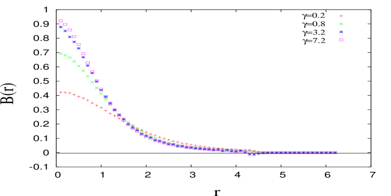
Figure 1: The magnetic field trapped in the vortex core for varying $\gamma$

4 The large coupling limit

Having presented a general algorithm for the construction of degree$-k$ semilocal vortex solutions of the gauged noncommutative linear sigma model and explicitly constructed the $1-$vortex solution we proceed now to study one of the more interesting limits of the semilocal model: its large coupling limit. At the level of the action (15), the $e^{2}\rightarrow\infty$ limit decouples the gauge field dynamics and any finite energy static solution has

$$E = 2\pi\vartheta{\rm Tr}_{\cal H}{\Bigl{[}}(\widehat{D}_{z}\widehat{\Phi})(\widehat{D}_{z}\widehat{\Phi})^{\dagger}+(\widehat{D}_{\bar{z}}\widehat{\Phi})(\widehat{D}_{\bar{z}}\widehat{\Phi})^{\dagger}{\Bigr{]}}$$ (30)

subject to the constraint $\widehat{\Phi}\widehat{\Phi}^{\dagger}=1$. In this limit, the gauge field is relegated to an auxiliary field, completely determined by $\Phi$. Recalling that $\Phi$ is an $(n+1)-$component complex vector leads to the conclusion that this is, of course, nothing but the noncommutative version of the $\mathbb{C}\mathbb{P}^{N}$ sigma model. At the level of the action this observation is certainly not new; in the commutative case, this relation has been commented on by several authors in many different contexts [16, 17, 30, 40]. However, it remains to be seen whether this correspondence persists at the level of the solutions. If it does we will have produced an explicit descent from the vortices of the fuzzy linear sigma model to the instantons of the noncommutative $\mathbb{C}\mathbb{P}^{N}$ model. In the interests of self-containment, we review now the derivation of the lump solutions of the sigma model.

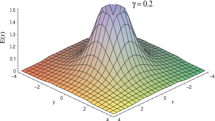
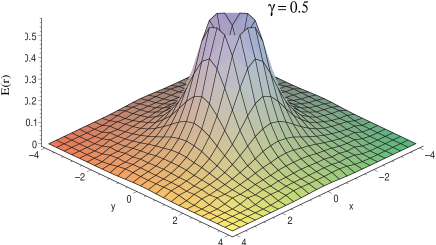
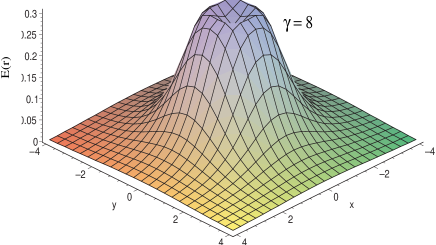
Figure 2: The metamorphosis of the semilocal vortex into the $\mathbb{C}\mathbb{P}^{N}$ lump

With eq.(30) as a starting point, a reparameterization of the $(N+1)-$component Higgs field as $\widehat{\Phi}=(1/\sqrt{\widehat{W}\widehat{W}^{\dagger}})\widehat{W}$ and subsequent definition of the Hermitian projector $P\equiv\widehat{W}^{\dagger}(\widehat{W}\widehat{W}^{\dagger})^{-1}\widehat{W}$ allows for the static energy (or two-dimensional action) to be written as

$$E=2\pi\,{\rm Tr}_{\cal H}{\rm tr}{\Bigl{(}}[P,\widehat{a}^{\dagger}][\widehat{a},P]{\Bigr{)}}.$$ (31)

In this form, the $\mathbb{C}\mathbb{P}^{N}$ energy is remarkably similar to the kinetic term of the static energy of a $(2+1)-$dimensional noncommutative scalar field (see eq.(2.2) of ref.[8]) with the crucial difference of the additional matrix trace in eq.(31). Indeed it was shown in [20, 21, 25] that the quantity ${\rm Tr}_{\cal H}{\rm tr}[\widehat{a},\widehat{a}^{\dagger}P]$ contributes a nonvanishing boundary term to the energy and some care needs to be exercised in the derivation of the noncommutative Bogomol’nyi bound. With this in mind, the energy may correctly be written as

$$E=2\pi\,{\rm Tr}_{\cal H}{\rm tr}{\Bigl{(}}2F_{+}(P)^{\dagger}F_{+}(P){\Bigr{)}}+2\pi Q_{+}\geq 2\pi Q_{+}$$ (32)

with the topological charge $Q_{+}\equiv{\rm Tr}_{\cal H}{\rm tr}(P-[\widehat{a},\widehat{a}^{\dagger}P])$ and $F_{+}(P)\equiv(1-P)\widehat{a}P$. A similar expression holds for the anti-BPS states. Focusing on the BPS states though, saturation of the bound on the energy is obtained when $F_{+}(P)=0$. As first shown in [22], solutions are not difficult to find; any Hermitian projector constructed from an $(n+1)-$vector $W$ whose components are holomorphic polynomials in $\widehat{z}$ will satisfy the above BPS equation. These are precisely the noncommutative extension of the instanton solutions of the conventional $\mathbb{C}\mathbb{P}^{N}$ sigma model. For example, the static, $1-$ and $2-$lump solutions of the noncommutative $\mathbb{C}\mathbb{P}^{1}$ model are given by

$$W_{1}={\Bigl{(}}\widehat{z}-a_{1}\,,\,b_{1}{\Bigr{)}}\qquad W_{2}={\Bigl{(}}\widehat{z}^{2}-a_{2}\,,\,2b_{2}\widehat{z}+c_{2}{\Bigr{)}}$$ (33)

where the soliton parameters $a_{1},...,d_{2}\in\mathbb{C}$ are chosen to coincide with the standard way of writing the solutions in the commutative theory [36]. These are the complex moduli of the $\mathbb{C}\mathbb{P}^{1}$ instanton. To facilitate comparison with the vortices, these may be written in the harmonic oscillator basis so that, for example, the $1-$lump solution becomes

$$W_{1}=\sum_{n=0}^{\infty}\sqrt{\frac{\vartheta(n+1)}{\vartheta(n+1)+1}}|n\rangle\langle n+1|\otimes\langle{\rm I}|+\sum_{n=0}^{\infty}\sqrt{\frac{1}{\vartheta(n+1)+1}}|n\rangle\langle n|\otimes\langle{\rm I\!I}|.$$ (34)

Returning to the degree$-k$ semilocal vortex of the last section, notice that eq.(23) may be recast as

$${\Bigl{(}}1+\frac{n!k!}{(n+k)!}\kappa^{2}{\Bigr{)}}Q_{n}-1+\frac{1}{\gamma}{\Bigl{(}}(n+k+1)\frac{Q_{n}}{Q_{n+1}}-(n+k)\frac{Q_{n-1}}{Q_{n}}-1{\Bigr{)}}=0\quad{}$$ (35)

In the infinite coupling limit $e^{2}\rightarrow\infty$ (or equivalently $\gamma\rightarrow\infty$), the above recurrence relation may be be solved exactly to give

$$Q_{n}={\Bigl{(}}1+\frac{n!k!}{(n+k)!}\kappa^{2}{\Bigr{)}}^{-1}.$$ (36)

In particular, for $k=1$ we find

$$Q_{n}=\frac{n+1}{n+1+\kappa^{2}}\qquad P_{n}=\frac{\kappa^{2}}{n+1+\kappa^{2}}.$$ (37)

Finally, matching coefficients to all orders in eqs.(34) and (37) means that the descent from noncommutative vortex to fuzzy lump only occurs when $\kappa^{2}=1/\vartheta$. Indeed, this is exactly the choice we made in our numerical computations to reduce the dimension of the shooting-parameter space. As a check, we expect that for a fixed value of $\vartheta$, $Q_{0}\rightarrow\vartheta/(\vartheta+1)$ as $\gamma\rightarrow\infty$. A quick glance at the table of our numerical results verifies that this is indeed the case for $\vartheta=0.2$ and $0.5$. Moreover, hindsight reveals that the set of energy densities in figure 2. is in fact a series of snapshots of the $k=1$ vortex of the noncommutative semilocal model morphing into a fuzzy $\mathbb{C}\mathbb{P}^{1}$ $1-$lump. The case $k=2$ is no less straightforward. With its center of mass localised at the origin, the $\mathbb{C}\mathbb{P}^{1}$ $2-$lump in eq.(33) can be written as

$$W_{2} = \sum_{n=0}^{\infty}\sqrt{\frac{\vartheta^{2}(n+1)(n+2)}{\vartheta^{2}(n+1)(n+2)+1}}|n\rangle\langle n+2|\otimes\langle{\rm I}|\qquad{}$$ (38)

$$+ \sum_{n=0}^{\infty}\sqrt{\frac{1}{\vartheta^{2}(n+1)(n+2)+1}}|n\rangle\langle n|\otimes\langle{\rm I\!I}|$$

when $b_{2}$, the frozen out modulus [5] is set to vanish. A comparison with the general expression for the infinite coupling coefficients (36) reveals a matching at all levels only if $\kappa^{2}=1/2\vartheta$. Generalisation to larger $k$ follows in much the same way so no further attention is paid to it here.

At this juncture, a few comments are in order. The Bogomol’nyi equations of the commutative gauged linear sigma model admit a one parameter family of vortex solutions [17]. This single complex parameter $w$ is to the commutative theory what the ratio of initial coefficients $\kappa$ is to our noncommutative model with $w=0$ corresponding to the conventional Neilsen-Olesen string. One of the distinguishing characteristics of the $w\neq 0$ semilocal vortices is the power law behavior exhibited by the scalar and gauge fields as they relax to their respective vacuum values. Consequently, the magnetic field $B\sim 2|w|^{2}/\xi^{4}$ and the width of the flux tube trapped in the vortex core is an arbitrary parameter instead of the Compton wavelength of the vector boson as in the Neilsen-Olesen vortex. In the noncommutative model we once again find a one parameter family of vortices only now the parameter, $\kappa$, is not at all arbitrary. Indeed, we find that there exists a point in the $\kappa$ parameter space dependent on the degree of the vortex and the deformation parameter $\vartheta$ at which the semilocal vortex exactly descends to the corresponding noncommutative $\mathbb{C}\mathbb{P}^{N}$ lump. Correspondingly, the width of the magnetic flux tube associated with the semilocal vortex is set by the scale of noncommutativity. This observed exact metamorphosis of the vortex into the lump should be compared to the results of section 3. of [17]. There an expansion of the $1-$instanton solution of the commutative $\mathbb{C}\mathbb{P}^{N}$ model in powers of $|w|/|z|$ was used to establish that the vortex-instanton matching was exact at spatial infinity with differences emerging at ${\cal O}(|w|^{4}/|z|^{4})$ in this expansion.

5 Brane Realisations

Quite apart from their intrinsic field theoretic value [35, 16, 17], the vortices of gauged linear sigma models also have a remarkably rich stringy structure. Beginning with the ground-breaking work of [11] in which the $(2+1)-$dimensional, ${\cal N}=4$ $U(N)$ Yang-Mills-Higgs theory was recognised as the worldvolume theory on a stack of $N$ $D3-$branes suspended between two parallel $NS5-$branes, an intricate tapestry of ideas can be woven, leading inexorably to a realisation of the noncommutative semilocal vortex as a $D-$brane configuration in type IIB string theory [10]. In this section, we review some of these ideas and cast them into a form that better facilitates comparison with our results.

As in [10] the description of the system begins with a $(2+1)-$dimensional, ${\cal N}=4$, $U(N)$ Yang-Mills-Higgs theory. The field content of the theory consists of a $U(N)$ vector multiplet made up of a gauge field $A_{\mu}$ and a triplet of adjoint scalars $\phi^{r}$ together with their fermionic super partners. Coupled to these are $N$ fundamental hypermultiplets each of which contain a doublet of complex scalars $q$ and $\widetilde{q}$ and their super partners. The Lagrangian for the theory is endowed with a global $SU(N+M)$ flavour symmetry as well as a local $U(N)$ gauge symmetry. Consequently, under these two groups and with $N_{f}\equiv N+M$ denoting the number of flavours, $q$ and $\widetilde{q}$ transform as $({\bf N},\overline{\bf N_{f}})$ and $(\overline{\bf N},{\bf N_{f}})$ respectively; the fundamental scalars are represented by $N\times(N+M)$ matrices. The dynamical content of the bosonic sector of the theory is contained in the Lagrangian

$${\cal L} = -{\rm Tr}{\Bigl{[}}\frac{1}{4e^{2}}F^{2}+\frac{1}{2e^{2}}(D\phi^{r})^{2}+(Dq)^{2}+(D\widetilde{q})^{2}+e^{2}|q\widetilde{q}|^{2}$$ (39)

$$+ \frac{1}{2e^{2}}[\phi^{r},\phi^{s}]^{2}+(q^{2}+\widetilde{q}^{2})\phi^{r}\phi^{r}+\frac{e^{2}}{2}(q^{2}-\widetilde{q}^{2}-\zeta{\bf 1}_{N}){\Bigr{]}}.$$

where the Fayet-Illiopolous (FI) parameter, $\zeta$, in the final D-term in (39) is chosen to be positive. This theory exhibits a Higgs branch of vacua which possess BPS vortices only if $\widetilde{q}$ and $\phi^{r}$ both vanish. This constraint defines a so-called reduced Higgs branch, ${\cal N}_{N,M}=Gr(N,N+M)$, the Grassmannian manifold of $N-$dimensional hyperplanes in $\mathbb{C}^{N+M}$. A particular vacuum choice is made by picking

$$q_{\rm vac} = \left\{\begin{array}[]{ll}\sqrt{\zeta}\delta^{a}_{i}&a,i=1,...,N\\ 0&i=N+1,...,N+M\end{array}\right.$$ (42)

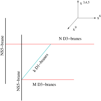
Figure 3: The degree$-k$ BPS vortex as $k$ stretched D-strings.

In our abelian case, for example, $N=1$, the reduced Higgs branch ${\cal N}_{1,M}=Gr(1,1+M)\simeq\mathbb{C}\mathbb{P}^{M}$ and $q_{\rm vac}=(\sqrt{\zeta},0)$. Relabeling $q\rightarrow\Phi$, setting the FI parameter $\zeta=1$ and restricting to time-independent solutions trivially establishes the equivalence of the action in this branch with the static energy (5). As discussed earlier, the spectrum of solutions of this theory is rich with BPS vortices. The brane realisation of these vortices is built up from the $U(N)$ Yang-Mills-Higgs described in (39). It consists of $N$ $D3-$branes suspended between two parallel $NS5-$branes and a further $N+M$ $D3$’s attached to the right hand $NS5-$brane to add flavour (see figure 3).

In the Higgs branch, one of the $NS5-$branes is separated from the others. This separation is proportional to the FI parameter $\zeta$. The degree$-k$ BPS vortices manifest as $k$ $D-$strings stretched between the $D3-$branes and the separated $NS5-$brane - an identification made on the basis of the fact that the stretched $D1-$branes are the only BPS states of the brane configuration with the correct mass. More than just a pretty picture, the geometry of the $D-$brane configuration in figure 3 encodes vital information about the FI parameter, $\zeta$ as well as the gauge coupling $e$ as

$$\frac{1}{e^{2}}=\frac{\Delta x^{6}}{2\pi g_{s}};\quad\zeta=\frac{\Delta x^{9}}{4\pi^{2}g_{s}l_{s}^{2}}$$ (43)

where $l_{s}$ and $g_{s}$ are the string length and coupling respectively and $\Delta x^{6}$ and $\Delta x^{9}$ are the separation distances between the $NS5-$branes defined as in figure 1. It is now clear that the sigma model limit ($e^{2}\rightarrow\infty$) of the vortex occurs precisely when the separation of the $NS5-$branes in the $6-$direction vanishes. The configuration that realises the $k-$lump solution of the (commutative) $\mathbb{C}\mathbb{P}^{M}$ nonlinear sigma model then is as above only with $N=1$. In string theory the transition from commutative to noncommutative worldvolume theories is achieved by turning on an NS-NS $B-$field in the appropriate direction [31]. In the present context, the transition from the semilocal action (5) to its noncommutative counterpart (15) translates into turning on a constant NS-NS $B-$field $B_{12}=\vartheta\,dx^{1}\wedge dx^{2}$ in the $(1,2)-$directions in a background of two $NS5-$branes with a $D3-$brane stretched between them and a further $M+1$ $D3$’s attached to the right hand $NS5-$brane. What of the vortices? The effect of the $B-$field on the $D-$strings stretched between the $NS5-$brane and the $D3$ is quite remarkable. The basic physics is analogous to the situation of a $D-$string suspended between two $D3-$branes studied in [15] and was first described for the vortex case in [10]. The NS-NS $2-$form manifests on the $D3-$worldvolume as a constant magnetic flux ${\cal F}_{12}$ while the $D-$string endpoint appears as a magnetic source. Since on the $4-$dimensional worldvolume of the $D3-$brane ${\cal F}_{12}=\star{\cal F}_{06}$, the magnetic endpoint of the $D1-$brane feels the same force as an electric charge in a constant electric field in the $6-$direction. However, as other end of the $D-$string remains married to the $NS5-$brane, the $D-$string responds to this force by tilting as in figure 4. The effect of the tilting was investigated in [15] by studying the $D-$string Born-Infeld action at weak string coupling

$$S=\frac{1}{2\pi l_{s}^{2}}\int_{0}^{\Delta x^{9}}\!\!dx^{9}\,{\Bigg{(}}\frac{1}{g_{s}}\sqrt{1+{\Bigl{(}}\frac{dx^{6}}{dx^{9}}{\Bigr{)}}^{2}}+A_{06}\frac{dx^{6}}{dx^{9}}{\Bigg{)}}$$ (44)

where the RR $2-$form $A_{06}$ that couples to the $D-$string worldvolume is induced by ${\cal B}_{06}$. The result of that investigation translated into the language of the vortex theory [10] is that the displacement of the $D1-$brane endpoint is given by $\delta=(\vartheta\Delta x^{9})/(2\pi l_{s}^{2})$. With this and some straightforward algebra, the distance between the $D-$string endpoint and the left $NS5-$brane can be computed. With the choice of $\zeta=1$ for the FI parameter, the result is

$$r=2\pi g_{s}{\Bigl{(}}\frac{1}{e^{2}}+\vartheta{\Bigr{)}}.$$ (45)

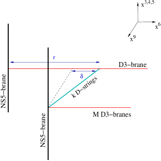
Figure 4: The magnetic field induced on the $D3-$worldvolume causes the $D-$strings to tilt.

This distance is, in fact, the FI parameter of the theory living on the $D1-$branes (see [10] for a lucid discussion of this aspect). Having fixed $\Delta x^{9}$ with the choice $\zeta=1$ the magnitude of $r$ is completely determined by the size of the gauge coupling as determined by the $NS5-$brane separation in the $6-$direction and the noncommutativity. Since the latter is also fixed, the transition from vortex to lump can be studied by changing the distance between the $NS5-$branes. As $\Delta x^{6}$ is decreased to zero, the separation between the $D-$string endpoint and the left $NS5-$brane decreases to $r_{*}=2\pi g_{s}\vartheta$. It is this configuration of the $k$ tilted $D-$strings stretched between the (formerly right hand) $NS5-$brane and the $D3-$brane that realises the degree$-k$ instanton of the $\mathbb{C}\mathbb{P}^{M}$ sigma model. This concludes our treatment of $D-$brane realisation of the noncommutative $\mathbb{C}\mathbb{P}^{M}$ lump.

More than just an academic exercise, this identification of the semilocal vortex and $\mathbb{C}\mathbb{P}^{M}$ instanton has proven invaluable in the understanding of the low energy dynamics of both the vortex and instanton as encoded in the geometry of their respective moduli spaces [34]. We refer the interested reader to [10] for a nice discussion of the structure of the moduli spaces and content ourselves with merely summarising some of their most pertinent results. The moduli space of degree$-k$ semilocal vortices $\hat{{\cal V}}_{k,(1,M)}$ is a $2k(1+M)-$dimensional space with a natural Kähler metric defined by the overlap of zero modes. However, this metric is afflicted with some non-normalisable zero modes that, classically, correspond to the moduli with infinite moments of inertia and that make the quantum mechanical treatment of these solitonic objects quite subtle. Fortunately these subtleties may be circumvented with a little help from the branes. A study of the theory on the $D1-$brane predicts that the Higgs branch, $\hat{\cal M}_{k,(1,M)}$, constructed by a $U(k)$ Kähler quotient of $\mathbb{C}^{k(1+M+k)}$ is isomorphic to the moduli space $\hat{{\cal V}}_{k,(1,M)}$. While the metric on $\hat{\cal M}_{k,(1,M)}$ retains all the symmetries of the Kähler metric on the vortex moduli space, it is finite and suffers from none of the non-normalisablity problems of the latter. Consequently, the study of the quantum theory of semilocal vortices may be simplified somewhat by replacing the natural metric on the vortex moduli space with the metric on the Higgs branch of the $D-$string theory inherited from the Kähler quotient construction of [10].

6 Conclusions and Discussion

The primary concern of this work has been the construction and study of a noncommutative extension of $(2+1)-$dimensional critically coupled, gauged linear sigma model. Like its commutative counterpart this theory possesses a rich spectrum of BPS solutions. By extending the systematic construction of [23] we have explicitly constructed a family of vortex solutions to the BPS equations (16) for arbitrary positive values of the noncommutativity parameter $\vartheta$. As expected, these fuzzy vortices reduce to the exact Neilsen-Olesen strings of the noncommutative Abelian-Higgs model [1, 2, 23, 37] on the co-dimension one surface $\kappa=0$ of the parameter space. Despite retaining many of the properties of their commutative cousins [17, 35], the introduction of a new length scale set by the noncommutativity parameter $\vartheta$ induces several remarkable differences. Among these we find that the width of the magnetic flux tube trapped in the vortex core no longer exhibits the characteristic arbitrariness of the commutative semilocal vortex. In the noncommutative model, this width is set by the scale of the noncommutativity.

The detailed investigation of the large coupling ($e^{2}\rightarrow\infty$) regime of the $\vartheta-$deformed gauged linear sigma model carried out in section 4. confirms, both numerically and analytically, the commutative intuition of the vortex morphing into a lump of the (fuzzy) $\mathbb{C}\mathbb{P}^{M}$ sigma model. Additionally, while the agreement between vortex and lump in the $\vartheta=0$ case is precise only asymptotically [17], we find an exact matching at all levels of the harmonic oscillator expansion at finite $\vartheta$. Indeed, insisting that this agreement holds selects a preferred set of values for $\kappa$, dependent on the scale of noncommutativity and the degree of the vortex. This effectively reduces the dimension of the parameter space by one. While we have explicitly constructed solutions for the $1-$ and $2-$vortex cases, the construction of higher degree solutions follows in much the same way and we do not expect any further surprises.

Finally, we reviewed the elegant constructions of [10] that lead to a realisation of the noncommutative $\mathbb{C}\mathbb{P}^{M}$ $k-$lump as $k$ tilted $D-$strings stretched between an isolated $NS5-$brane (on which a stack of $M$ semi-infinite $D3-$branes end) and a semi-infinite $D3$ whose one endpoint ends on a second $NS5$ (see figure 4). This identification is built on the foundation of a study of the ${\cal N}=4$ $U(N)$ Yang-Mills-Higgs $D3-$worldvolume theory hinges on the metamorphosis of vortices into lumps. Of course, to be sure that this configuration really does correspond to the lump solution requires more work than just a comparison of the masses of both configurations; the spectrum of fluctuations around each object needs to be computed and compared. This is a more difficult endeavor which, together with a more thorough investigation of the spectrum of BPS objects of the noncommutative gauged linear sigma model is left to future work [26]. Curiously, this realisation of fuzzy $\mathbb{C}\mathbb{P}^{M}$ lumps is not unique, at least for $M=1$. Drawing on the tree level equivalence between ${\cal N}=2$ open string theory and self-dual Yang-Mills theory in $(2+2)-$dimensions [29], it was argued in [20, 21] that the effective field theory induced on the worldvolume of $N$ $D2-$branes by ${\cal N}=2$ open strings in a Kähler $B-$field background is a noncommutative $U(N)$ sigma model. Using a modified “method of dressing” soliton solutions of the latter were constructed and their various scattering properties investigated. In this context, the $k-$lump solution of the $\mathbb{C}\mathbb{P}^{1}$ sigma model may be interpreted as $k$ $D0-$branes in the worldvolume of a stack of $D2-$branes [21, 18]. Again, while this assertion needs to be tested beyond the level of a mass comparison, the possibility of a duality between ${\cal N}=2$ open string theory and the type II-B superstring is, to say the least, intriguing and certainly deserves more attention.

- [1] D. Bak, “Exact Multivortex Solutions in Noncommutative Abelian Higgs Theory” Phys. Lett. B 495, 251-255, (2000), hep-th/0008204
- [2] D. Bak, K. Lee and J-H. Park, “Noncommutative Vortex Solitons” Phys. Rev. D 63, 125010 (2001), hep-th/0011099
- [3] H. de Vega and F. Schaposnik, “A classical vortex solution of the of the Abelian-Higgs model” Phys. Rev. D 14, 1100 (1976)
- [4] M.R. Douglas and N.A. Nekrasov , “Noncommutative Field Theory” Rev. Mod. Phys 73, 977 (2001), hep-th/0106048
- [5] K. Furuta, T. Inami, H. Nakajima and M. Yamamoto, “Low-energy dynamics of noncommutative solitons in dimensions,” Phys. Lett. B 537, 165-172, (2002), hep-th/0203125
- [6] K. Furuta, T. Inami, H. Nakajima and M. Yamamoto, “Non-BPS Solutions of the Noncommutative Model in -dimensions,” JHEP 0208, 009, (2002), hep-th/0207166
- [7] R. Gopakumar , S. Minwalla and A. Strominger, “Noncommutative Solitons” JHEP 0005, 020 (2000), hep-th/0003160
- [8] R. Gopakumar, M. Headrick and M. Spradlin, “On Noncommutative Multisolitons.” (2001), hep-th/0103256
- [9] D.J. Gross and N.A. Nekrasov, “Solitons in noncommutative gauge theory.” JHEP 0103, 044 (2001), hep-th/0010090
- [10] A. Hanany and D. Tong, “Vortices, Instantons and Branes” hep-th/0306150
- [11] A. Hanany and E. Witten, “Type IIB superstrings, BPS monopoles, and three-dimensional gauge invariance” Nucl. Phys. B 492, 152 (1997) hep-th/9611230
- [12] J.A. Harvey, “Komaba Lectures on Noncommutative Solitons and D-Branes,” (2001), hep-th/0102076
- [13] J.A. Harvey, P. Kraus, F. Larsen and E. J. Martinec, “D-Branes and Strings as Non-commutative solitons,” JHEP 0007, 042 (2000), hep-th/0005031
- [14] J.A. Harvey, P. Kraus and F. Larsen, “Exact Noncommutative Solitons,” JHEP 0012, 024 (2000), hep-th/0010060
- [15] A. Hashimoto and K. Hashimoto, “Monopoles and dyons in noncommutative geometry” JHEP 11, 005 (1999) hep-th/9909202
- [16] M. Hindmarsh, “Existence and Stability of Semilocal Strings” Phys. Rev. Lett. 68, 9 (1992)
- [17] M. Hindmarsh, “Semilocal Topological Defects” Nucl. Phys. B 392, 461 (1993) hep-ph/9206229
- [18] M. Ihl and S. Uhlmann, “Noncommutative Extended Waves and Soliton-like Configurations in N=2 String Theory,” (2002), hep-th/0211263
- [19] O.Lechtenfeld and A.D.Popov, “Noncommutative Multi-solitons in 2+1 dimensions” JHEP 0111, 040 (2001), hep-th/0106213
- [20] O.Lechtenfeld and A.D.Popov, “Scattering of Noncommutative Solitons in 2+1 dimensions” Phys. Lett. B 523, 178-184 (2001), hep-th/0108118
- [21] O.Lechtenfeld, A.D.Popov and B. Spendig, “Noncommutative Solitons in Open N=2 String Theory” JHEP 0106, 011 (2001), hep-th/0103196
- [22] B-H. Lee, K. Lee and H.S. Yang, “The model on noncommutative plane” Phys. Lett B 498, 277-284 (2001), hep-th/0007140
- [23] G.S. Lozano, E.F. Moreno and F.A. Schaposnik, “Nielsen-Olesen vortices in noncommutative space” Phys. Lett B 504, 117 (2001), hep-th/0011205
- [24] N.S. Manton, “A remark on the scattering of BPS monopoles” Phys. Lett B 110, 54 (1982)
- [25] J. Murugan and R. Adams, “Comments on Noncommutative Sigma Models” JHEP 0212, 073 (2002), hep-th/0211171
- [26] J. Murugan and A. Millner, In progress
- [27] N.A. Nekrasov, “Noncommutative instantons revisited.” (2000), hep-th/0010017
- [28] H.B. Nielsen and P. Olesen, “Vortex line models for dual strings” Nucl. Phys. B 61, 45 (1973)
- [29] H. Ooguri and C. Vafa, “Geometry of N=2 Strings” Nucl. Phys. B 361, 469-518 (1991)
- [30] B.J. Schroers, “The Spectrum of Bogomol’nyi solitons in gauged linear sigma models” Nucl. Phys. B 475, 440-468 (1996), hep-th/0210010
- [31] N. Seiberg and E. Witten, “String Theory and Noncommutative Geometry” JHEP 09, 032 (1999), hep-th/9908142
- [32] I. Strachan, “Low velocity scattering of vortices in a modified Abelian-Higgs model” J. Math. Phys. 33, 102 (1992)
- [33] R.J. Szabo, “Quantum Field Theory on Noncommutative Spaces” Phys. Rep. 378, 207 (2003)
- [34] D. Tong, “The Moduli Space of Noncommutative Vortices” J. Math. Phys. 44, 3509 (2003) hep-th/0210010
- [35] T. Vachaspati and A. Achucarro, “Semilocal cosmic strings” Phys. Rev. D 44, 3067 (1991)
- [36] R.S. Ward, “Slowly moving lumps in the model in dimensions” Phys. Lett B 158, 424 (1985)
- [37] D. Jatkar, G. Mandal and S. Wadia, “Nielsen-Olesen Vortices in Noncommutative Abelian Higgs Model” JHEP 0009, 018 (2000), hep-th/0007078
- [38] E. Witten, “Some exact multi-instanton solutions of classical Yang-Mills theory” Phys. Rev. Lett. 38, 121 (1977)
- [39] E. Witten, “Noncommutative Geometry and String Field Theory” Nucl. Phys. B 268, 253 (1986)
- [40] E. Witten, “Phases of theories in two dimensions” Nucl. Phys. B 403, 159 (1993)