A new duality relating density perturbations in
expanding and contracting Friedmann cosmologies

Abstract

For a 4–dimensional spatially-flat Friedmann-Robertson-Walker universe with a scalar field $\phi(x)$, potential $V(\phi)$ and constant equation of state $w=p/\rho$, we show that an expanding solution characterized by $\epsilon=3(1+w)/2$ produces the same scalar perturbations as a contracting solution with $\widehat{\epsilon}=1/\epsilon$. The same symmetry applies to both the dominant and subdominant scalar perturbation modes. This result admits a simple physical interpretation and generalizes to $d$ spacetime dimensions if we define $\epsilon\equiv[(2d-5)+(d-1)w]/(d-2)$.

I Introduction

In inflationary cosmology inflation , a nearly scale-invariant spectrum of primordial density perturbations is produced as comoving scales leave the Hubble horizon during an early burst of accelerated expansion inflation_perts . In cyclic cosmology cyclic_ekpyrotic , the same perturbation spectrum is produced as comoving scales leave the Hubble horizon during a period of slow decelerated contraction cyclic_perts ; TTS . This agreement between two physically dissimilar models is unexpected, but not coincidental. As we shall show, the relationship between inflation and the cyclic model may be viewed as a special case of a surprisingly simple and general duality between expanding and contracting cosmologies.

A Friedmann-Robertson-Walker (FRW) universe with a single scalar field $\phi$ and potential $V(\phi)$ is a simple yet important system. In particular, it is the canonical 4d effective theory used to model the production of density perturbations in both inflationary and cyclic cosmology. Recent results hint at a connection between two apparently–unrelated regimes of this model: (i) expanding, in the $w\rightarrow-1$ limit, and (ii) contracting, in the $w\rightarrow\infty$ limit. Here $w\equiv p/\rho$ denotes the ratio of pressure to energy density. Long-wavelength scale-invariant density perturbations are produced in the limits (i) and (ii) PHZ_conditions , and the small deviations from scale invariance near these two limits are related by the simple substitution $\epsilon\rightarrow 1/\epsilon$, where $\epsilon\equiv 3(1+w)/2$ spectral_tilt .

The relationship noted in PHZ_conditions ; spectral_tilt between expanding $w\approx-1$ models and contracting $w\gg 1$ models, turns out to be a special case of a general and exact duality relating expanding and contracting models with identical perturbation spectra. In this paper, we derive this duality, focusing on the case where $\epsilon$ (or $w$) is time-independent. In a companion paper dual2 , we generalize the discussion to the case where $\epsilon$ is time-varying. When $\epsilon$ is constant, or varies sufficiently slowly, the duality is simple: an expanding universe characterized by $\epsilon$ produces exactly the same scalar perturbations as a contracting universe characterized by $\widehat{\epsilon}=1/\epsilon$. This duality applies in arbitrary spacetime dimension (not just 3+1); it applies for all $w$ (not just the $w\rightarrow-1$ and $w\rightarrow\infty$ limits discussed in PHZ_conditions ; spectral_tilt ); it applies to all wavelengths (not just the long-wavelength limit); it applies to both the dominant scalar perturbation mode and a subdominant remainder (which are related to the growing and decaying modes, respectively).

This duality is of general theoretical interest since it provides a new relationship between expanding and contracting universes, and exposes an unexpected symmetry of cosmological perturbation theory. It is also relevant to cosmological models, like the ekpyrotic and cyclic cyclic_ekpyrotic scenarios, in which perturbations produced during a period of contraction are proposed to propagate through a bounce into a subsequent expanding phase. These models require that the growing-mode long-wavelength perturbation spectrum is preserved across the bounce. This has been a controversial matter. At first, some authors argued that growing-mode perturbations produced in a contracting phase must match to pure decaying-mode perturbations as one follows them across a bounce into an expanding phase contrascale . At heart, this conclusion followed from requiring that the bounce corresponds to a comoving or constant-energy-density slice. However, recent five dimensional calculations TTS ; newbrand indicate that comoving or constant-energy-density slices are inappropriate for matching, since the bounce event (represented in five dimensions by a brane collision) is not synchronous in these slices. Matching on collision-synchronous slices results in the propagation of growing-mode perturbations across a bounce, with no change in the shape of the long-wavelength spectrum. Other aspects of the cyclic and ekpyrotic models have been criticized kallosh (see ansc for replies), and some have argued that a bounce is impossible altogether contrabounce . While the consistency of a bounce remains to be proven, recent work has shown that the traditional hazard of chaotic mixmaster behavior is strongly suppressed in the contracting phase of the cyclic model chaos . The metric perturbations exhibit ultralocal behavior in which anisotropies remain small, right up to a few Planck times before the bounce. In this situation, causality suggests that the bounce should not disturb correlations on macroscopic scales over which there can be no communication in this finite time interval. Under these conditions, works by several groups TTS ; pro ; newbrand suggest that perturbations generated during the contracting phase may pass into the expanding phase. The subject continues to be an area of active research. If the latter suggestions are made rigorous, it would give added significance to the results presented herein.

Other dualities have been identified in the literature Wands ; Starobinsky ; Brustein ; scalefacdual ; stringdual that relate cosmological solutions and perturbations. See Section VI for a comparison. The duality presented here has the distinctive property that it relates two solutions that are stable under perturbations. Hence, both solutions can plausibly play a role in realistic cosmological models.

The layout of the paper is as follows. In section II, we introduce the background (unperturbed) model: a spatially-flat FRW model with scalar field $\phi$, potential $V(\phi)$, and constant $\epsilon$. In section III, we briefly review scalar perturbation theory, before deriving exact solutions for Mukhanov’s $u$ and $v$ variables. We note that $u$ is invariant under $\epsilon\rightarrow 1/\epsilon$. This invariance is independent of our vacuum choice for the fluctuations, and provides our first glimpse of the duality. In section IV we use $u$ and $v$ to separate scalar perturbations into pieces that are dominant and subdominant at long wavelengths, and show that each piece is both independently invariant under $\epsilon\to 1/\epsilon$. We show how the dominant and subdominant pieces relate to the scalar perturbation growing and decaying modes. In section V we consider tensor perturbations. In section VI, we contrast our duality with other kinds of cosmological dualities that have been studied in the literature Wands ; Starobinsky ; Brustein ; scalefacdual ; stringdual . In section VII, we interpret our duality as a relation between the scale factor and the Hubble parameter, discuss its observational significance, and mention some open questions. In an appendix, we generalize our results to $d$ spacetime dimensions.

II Background model

A spatially-flat Friedmann-Robertson-Walker (FRW) universe with scalar field $\phi$ and potential $V(\phi)$ is described by the metric

$$\textrm{d}s^{2}=a(\tau)^{2}\left[-\textrm{d}\tau^{2}+\textrm{d}\vec{x}^{\,2}\right].$$ (1)

The unperturbed scalar field $\phi_{0}(\tau)$ and scale factor $a(\tau)$ obey the Friedmann equations

$$6(a^{\prime\,2}/a^{4}) = 2\rho$$ (2a)

$$6(a^{\prime\prime}/a^{3})\; = \rho-3p$$ (2b)

where we have chosen units such that $c=\hbar=8\pi G=1$, a prime ($\,{}^{\prime}\,$) denotes a conformal time derivative $\textrm{d}/\textrm{d}\tau$, and the energy density and pressure are given by

$$\rho = (1/2)a^{-2}\phi_{0}^{\prime\,2}+V(\phi_{0})$$ (3a)

$$p = (1/2)a^{-2}\phi_{0}^{\prime\,2}-V(\phi_{0}).$$ (3b)

Instead of the usual variable $w\equiv p/\rho$, it will be more convenient to use

$$\epsilon\equiv 3(1+w)/2.$$ (4)

to parameterize the equation of state. Equations (2,3) imply $-1\leq w<\infty$ (or equivalently $0\leq\epsilon<\infty$). If $w$ is near $-1$, then $\epsilon\ll 1$ is the usual slow-roll parameter; but we make no slow-roll approximation in this paper, and $\epsilon$ may be arbitrarily large.

From now on, we shall assume that $\epsilon$ is constant, not equal to unity. (The self-dual case $\epsilon=1$ possesses special behavior which we shall not study here.) Then the solution of equations (2,3) is:

$$a(\tau) = |\tau|^{1/(\epsilon-1)}$$ (5a)

$$\phi_{0}(\tau) = \pm\frac{(2\epsilon)^{1/2}}{\epsilon-1}\,\textrm{ln}|\tau|$$ (5b)

$$V(\phi) = \frac{3-\epsilon}{(\epsilon-1)^{2}}\,\textrm{exp}\!\!\left[\mp(2\epsilon)^{1/2}\phi\right]$$ (5c)

where, to fix integration constants we have, without loss of generality, chosen the origin of conformal time so that $a(0)=0$, normalized the scale factor so that $a(1)=1$, and redefined $\phi_{0}\rightarrow\phi_{0}+$constant so that $\phi_{0}(1)=0$.

This solution separates into 4 cases:

• (a) expanding, $0\leq\epsilon<1$, $-\infty<\tau<0$;

• (b) expanding, $1<\epsilon<\infty$, $0<\tau<\infty$;

• (c) contracting, $0\leq\epsilon<1$, $0<\tau<\infty$;

• (d) contracting, $1<\epsilon<\infty$, $-\infty<\tau<0$.

Figure 1: Penrose diagrams for spatially-flat FRW universes with: (a) $0<\epsilon<1$, expanding; (b) $1<\epsilon<\infty$, expanding; (c) $0<\epsilon<1$, contracting; (d) $1<\epsilon<\infty$, contracting. The left edge of each diagram is the world line of a comoving observer at the origin; curved lines represent other comoving world lines and spatial hypersurfaces. The Hubble horizon is a curve connecting the $90^{o}$ vertex to the lightlike boundary, but the precise curve depends on $\epsilon$. For illustration, we have shown the horizon for $\epsilon=0$ in (a, c) and for $\epsilon=2$ in (b, d). In this paper, we focus on cases (a) and (d), in which comoving scales exit the Hubble horizon.

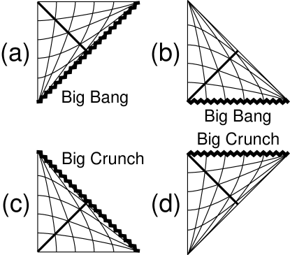
The Penrose diagrams for these 4 possibilities are shown in Figure 1. Case (b) corresponds to an ordinary expanding FRW model with matter or radiation domination, $\epsilon=3/2$ or $2$, respectively. We are interested in the two cases, (a) and (d), in which $\tau$ runs from $-\infty\rightarrow 0$ since, in these two cases, comoving length scales start inside the Hubble horizon at early times, and end outside the horizon at late times. Since we wish to study the amplification of perturbations as modes leave the horizon, these are the two relevant cases. Thus, we will always assume $\epsilon<1\Leftrightarrow\textrm{expanding}$ and $\epsilon>1\Leftrightarrow\textrm{contracting}$. The duality discussed below pairs solutions of type (a) with solutions of type (d). Figure (1) emphasizes that (a) and (d) have similar causal structure, but different singularities.

III Scalar perturbations

In this section, we introduce relevant aspects of gauge-invariant scalar perturbation theory in 4 dimensions, and catch our first glimpse of the duality discussed in section IV. For a thorough introduction to gauge-invariant perturbations Bardeen , see Kodama_Sasaki and pert_reviews . We work in Fourier space throughout, so every perturbation variable carries an implicit subscript $\vec{k}$ which, for brevity, is not shown explicitly. Write the perturbed metric

$$\textrm{d}s^{2}/a^{2} = -(1+2AY)\textrm{d}\tau^{2}-2BY_{i}\textrm{d}\tau\textrm{d}x^{i}$$ (6a)

$$+\left[(1+2H_{L}Y)\delta_{ij}+2H_{T}Y_{ij}\right]\textrm{d}x^{i}\textrm{d}x^{j}$$

and perturbed scalar field

$$\phi=\phi_{0}(\tau)+\delta\phi(\tau)Y$$ (6b)

where $Y(\vec{x})$, $Y_{i}(\vec{x})$, and $Y_{ij}(\vec{x})$ are scalar harmonics (see Appendix C in Kodama_Sasaki ). The corresponding perturbations of the Einstein tensor and energy-momentum tensor (see Appendices D and F in Kodama_Sasaki ) are related to one another through the perturbed Einstein equations, $\delta G^{\mu}_{\;\;\nu}=\delta T^{\mu}_{\;\;\nu}$.

It is well known that scalar perturbations in a spatially-flat FRW universe with scalar field $\phi$ and potential $V(\phi)$ are completely characterized by a single gauge-invariant variable. But the choice of this variable is neither unique nor standard; two of the most familiar options are the “Newtonian potential,” $\Phi$, and the “curvature perturbation,” $\zeta$.

The gauge-invariant Newtonian potential $\Phi$ is most easily understood in “Newtonian gauge” ($B\!=\!H_{T}\!=\!0$), where it is related to the metric perturbations in a simple way: $\Phi=A=-H_{L}$. It obeys the equation of motion

$$\Phi^{\prime\prime}+2\left[\frac{a^{\prime}}{a}-\frac{\phi_{0}^{\prime\prime}}{\phi_{0}^{\prime}}\right]\Phi^{\prime}+2\left[k^{2}+2\mathcal{H}^{\prime}-2\mathcal{H}\frac{\phi_{0}^{\prime\prime}}{\phi_{0}^{\prime}}\right]\Phi=0$$ (7)

where $k=|\vec{k}|$ is the magnitude of the (comoving) Fourier 3-vector. On the other hand, the gauge-invariant perturbation variable $\zeta$ is most easily understood in “comoving gauge” ($H_{T}=\delta T^{0}_{\;\;i}=0$), where it represents the curvature perturbation on spatial-hypersurfaces, and is related to the spatial metric perturbation in a simple way: $\zeta=-H_{L}$. The condition $\delta T^{0}_{\;\;i}=0$ also implies that $\delta\phi=0$ in this gauge. $\zeta$ obeys the equation of motion

$$\zeta^{\prime\prime}+2(z^{\prime}/z)\zeta^{\prime}+k^{2}\zeta=0$$ (8)

where $z\equiv a^{2}\phi_{0}^{\prime}/a^{\prime}$. $\Phi$ and $\zeta$ are related to each other by

$$\zeta = \Phi+\frac{1}{\epsilon}\left[(a/a^{\prime})\Phi^{\prime}+\Phi\right]$$ (9a)

$$\Phi = -\epsilon(a^{\prime}/a)k^{-2}\zeta^{\prime}\;.$$ (9b)

Note that our definitions for $\Phi$ and $\zeta$ agree with those in pert_reviews . But beware: in Kodama_Sasaki , the gauge-invariant Newtonian potential is denoted $\Psi$, while $\Phi$ denotes a different (though closely related) variable.

It is convenient to introduce new variables, $u$ and $v$ Mukhanov , by multiplying $\Phi$ and $\zeta$ by $k$-independent functions of $\tau$:

$$u\equiv(a/\phi_{0}^{\prime})\Phi\qquad v\equiv z\zeta.$$ (10)

Note that $u$ and $v$ have the same $k$-dependence as $\Phi$ and $\zeta$, respectively, and may serve as surrogates for $\Phi$ and $\zeta$. If we also define background quantities, $\theta$ and $z$:

$$\theta\equiv 1/z\equiv\frac{a^{\prime}}{a^{2}\phi_{0}^{\prime}},$$ (11)

then $u$ and $v$ obey simple equations of motion

$$u^{\prime\prime}+(k^{2}-\theta^{\prime\prime}/\theta)u = 0$$ (12a)

$$v^{\prime\prime}+(k^{2}-z^{\prime\prime}/z)v = 0$$ (12b)

and are related to each other by

$$kv = 2k[u^{\prime}+(z^{\prime}/z)u]$$ (13a)

$$-ku = \frac{1}{2k}[v^{\prime}+(\theta^{\prime}/\theta)v].$$ (13b)

We must choose a vacuum state for the fluctuations, which corresponds to specifying appropriate boundary conditions for $u$ and $v$ (see Ch.3 in Birrel&Davies Birrell_Davies ). The standard choice is the Minkowski vacuum of a comoving observer in the far past (when all comoving scales were far inside the Hubble horizon), corresponding to the boundary conditions

$$u \rightarrow i(2k)^{-3/2}\textrm{e}^{-ik\tau}$$ (14a)

$$v \rightarrow\;(2k)^{-1/2}\textrm{e}^{-ik\tau}$$ (14b)

as $\tau\rightarrow-\infty$. Using (13), it is easy to check that these two boundary conditions are equivalent.

When $\epsilon$ is time-independent, we can use (5) to find

$$\theta^{\prime\prime}/\theta = \frac{\epsilon}{(\epsilon-1)^{2}\tau^{2}}$$ (15a)

$$z^{\prime\prime}/z = \frac{2-\epsilon}{(\epsilon-1)^{2}\tau^{2}}$$ (15b)

Then we may solve (12) to obtain

$$u(x)=x^{1/2}\left[A^{(1)}H^{(1)}_{\alpha}(x)+A^{(2)}H^{(2)}_{\alpha}(x)\right]$$ (16a)

$$v(x)=x^{1/2}\left[B^{(1)}H^{(1)}_{\beta}(x)+B^{(2)}H^{(2)}_{\beta}(x)\right]$$ (16b)

where $x\equiv k|\tau|$ is a dimensionless time variable, $A^{(1,2)}$ and $B^{(1,2)}$ are constants, $H^{(1,2)}_{\rho}(x)$ are Hankel functions, and we have defined

$$\alpha\equiv \sqrt{(\theta^{\prime\prime}/\theta)\tau^{2}+1/4} =\frac{1}{2}\left|\frac{\epsilon+1}{\epsilon-1}\right|$$ (17a)

$$\beta\equiv \sqrt{(z^{\prime\prime}/z)\tau^{2}+1/4} =\frac{1}{2}\left|\frac{\epsilon-3}{\epsilon-1}\right|$$ (17b)

In the far past ($x\rightarrow\infty$) we use the asymptotic Hankel expression,

$$H^{(1,2)}_{s}(x)\rightarrow\sqrt{\frac{2}{\pi x}}\textrm{exp}\left[\pm\,i\left(x-\frac{s\,\pi}{2}-\frac{\pi}{4}\right)\right]$$ (18)

so the boundary conditions (14) imply

$$u = \frac{\mathcal{P}_{1}}{2k}(\pi x/4k)^{1/2}H_{\alpha}^{(1)}(x)$$ (19a)

$$v = \,\mathcal{P}_{2}\,(\pi x/4k)^{1/2}H_{\beta}^{(1)}(x)$$ (19b)

where

$$\mathcal{P}_{1}=\textrm{exp}[i(2\alpha+3)\pi/4]$$ (20a)

$$\mathcal{P}_{2}=\textrm{exp}[i(2\beta+1)\pi/4]$$ (20b)

are $k$-independent complex phase factors.

Note from (15a) that the equation of motion for $u$, (12a), is invariant under $\epsilon\rightarrow 1/\epsilon$, while the boundary condition, (14a), is independent of $\epsilon$. As a result, our expressions (17a) for $\alpha$ and (19a) for $u$ are invariant under $\epsilon\rightarrow 1/\epsilon$. This is our first glimpse of the duality discussed below.

We stress that this result does not depend on the particular vacuum choice (14a). Any boundary condition that is independent of $\epsilon$ (or, more generally, invariant under $\epsilon\rightarrow 1/\epsilon$) will work. And it is natural to expect the boundary condition to be independent of $\epsilon$, since it is imposed in the far past, when comoving scales are far inside the Hubble horizon.

IV Dominant and subdominant modes

In this section, we show that $u$ and $v$ can be decomposed into pieces that are dominant and subdominant at long wavelengths such that each is invariant under the transformation $\epsilon\rightarrow 1/\epsilon$. The dominant and subdominant parts are closely related growing and decaying modes over the range of $w$ relevant to cosmological model-building, as we explain below.

For this analysis, it is convenient to scale $u$ and $v$ by appropriate powers of $|\tau|$, so that they only depend on $k$ and $\tau$ through the dimensionless combination $x=k|\tau|$. Thus, using (19a, 19b), define

$$\bar{u}\equiv|\tau|^{-3/2}u = \frac{\mathcal{P}_{1}}{2x}(\pi/4)^{1/2}H_{\alpha}^{(1)}(x)$$ (21a)

$$\bar{v}\equiv|\tau|^{-1/2}v = \,\mathcal{P}_{2}\,(\pi/4)^{1/2}H_{\beta}^{(1)}(x).$$ (21b)

Note that $\bar{u}$ and $\bar{v}$ have the same $k$-dependence as $u$ and $v$, respectively, or $\Phi$ and $\zeta$, respectively, and may be used in place of these more standard variables.

To make the meaning of “dominant” and “subdominant” precise, consider two linearly independent functions $f_{1}(x)$ and $f_{2}(x)$. If $\lim_{x\to 0}f_{2}(x)/f_{1}(x)$ exists, then $f_{1}(x)$ and $f_{2}(x)$ can be related by a linear transformation to two new functions, $f_{{\rm dom}}(x)$ and $f_{{\rm sub}}(x)$, satisfying

$$\lim_{x\to 0}f_{{\rm sub}}(x)/f_{{\rm dom}}(x)=0.$$ (22)

So the subdominant piece, $f_{{\rm sub}}(x)$, becomes negligible relative to the dominant piece, $f_{{\rm dom}}(x)$, for small $x$ (i.e. far outside the horizon). The condition (22) uniquely determines the subdominant piece (up to an overall normalization constant) to be

$$f_{{\rm sub}}(x)=f_{2}(x)-\left[\lim_{y\to 0}\frac{f_{2}(y)}{f_{1}(y)}\right]f_{1}(x),$$ (23)

but does not uniquely fix the dominant piece. Rather, $f_{{\rm dom}}(x)$ may be any linear combination of $f_{1}(x)$ and $f_{2}(x)$ that is linearly independent of $f_{{\rm sub}}(x)$. We can now choose $f_{1}(x)=\bar{u}(x)$ and $f_{2}(x)=\bar{v}(x)$, and find the corresponding dominant and subdominant functions.

Let us first calculate $f_{{\rm sub}}(x)$. To compute $\lim_{x\to 0}f_{2}(x)/f_{1}(x)$, recall the Hankel identity

$$H_{s}^{(1)}(x)\rightarrow-i[\Gamma(s)/\pi](x/2)^{-s}\quad\textrm{as}\quad x\rightarrow 0,$$ (24)

where $s>0$ and $\Gamma(s)$ is the Euler gamma function. Then from (21a,21b) we find

$$\lim_{x\to 0}\frac{f_{2}(x)}{f_{1}(x)}=\left\{\begin{array}[]{ll}(\mathcal{P}_{2}/\mathcal{P}_{1})4\alpha&0\leq\epsilon<1\\ 0&1<\epsilon<\infty\end{array}\right.$$ (25)

where we have used the fact that $\alpha+1=\beta$ when $\epsilon<1$, while $\alpha+1>\beta$ when $\epsilon>1$. Now, substituting (21a), (21b) and (25) into (23), using the Hankel identities

$$H_{s-1}^{(1)}(x)+H_{s+1}^{(1)}(x)=\frac{2s}{x}H_{s}^{(1)}(x)$$ (26a)

$$H_{-s}^{(1)}(x)=\textrm{e}^{i\pi s}H_{s}^{(1)}(x),$$ (26b)

and paying careful attention to absolute value signs, we find

$$f_{{\rm sub}}(x)=\mathcal{P}_{3}(\pi/4)^{1/2}H_{\gamma}^{(1)}(x),$$ (27)

where we have defined

$$\gamma\equiv|\alpha-1|,$$ (28)

and $\mathcal{P}_{3}=\textrm{exp}[i(2\gamma+1)\pi/4]$ is a $k$-independent complex phase factor.

Now let us turn to $f_{{\rm dom}}(x)$. The fact that $\lim_{x\to 0}f_{{\rm sub}}(x)/\bar{v}(x)=0$ when $\epsilon<1$ shows that the dominant mode contributes to $\bar{v}$ in an expanding universe. Since $f_{{\rm sub}}(x)=\bar{v}(x)$ when $\epsilon>1$, $\bar{v}$ is purely subdominant (i.e. contains no dominant-mode contribution) in a contracting universe. By contrast, $\bar{u}$ and $f_{s}(x)$ are always linearly independent, and hence $\lim_{x\to 0}f_{{\rm sub}}(x)/\bar{u}(x)=0$ for all $\epsilon$. Thus, we can use the freedom in defining $f_{{\rm dom}}$ to choose

$$f_{{\rm dom}}(x)=\bar{u}(x)=\frac{\mathcal{P}_{1}}{2x}(\pi/4)^{1/2}H_{\alpha}^{(1)}(x)$$ (29)

for the dominant piece.

Notice that the expressions (27) for $f_{{\rm sub}}(x)$ and (29) for $f_{{\rm dom}}(x)$ are both invariant under $\epsilon\rightarrow 1/\epsilon$, because $\alpha$ is invariant. Thus, we see that the subdominant mode automatically possesses this symmetry, since $f_{{\rm sub}}(x)$ is uniquely determined (up to a normalization factor) by the condition (22). Furthermore, we have shown that we can choose a linear combination of $\bar{u}(x)$ and $\bar{v}(x)$ such that $f_{{\rm dom}}(x)$ displays the same symmetry. (If we had made the wrong choice for $f_{{\rm dom}}(x)$, then the exact $\epsilon\rightarrow 1/\epsilon$ symmetry of the dominant mode would be hidden, and would only re-appear in the long-wavelength limit.)

In the $x\rightarrow 0$ limit, define dominant and subdominant scalar spectral indices, $n_{{\rm dom}}$ and $n_{{\rm sub}}$, which satisfy

$$x^{3}|f_{{\rm dom}}|^{2} \propto x^{n_{{\rm dom}}-1}$$ (30a)

$$x^{3}|\,f_{{\rm sub}}\,|^{2} \propto x^{n_{{\rm sub}}-1}$$ (30b)

Using (27) and (29), along with the Hankel identity (24), we find

$$n_{{\rm dom}}-1\!\! =1-2\alpha=\! 1-\;\Big{|}\frac{\epsilon+1}{\epsilon-1}\Big{|}$$ (31a)

$$n_{{\rm sub\;}}-1\!\! =3-2\gamma=\! 3-\left|\Big{|}\frac{\epsilon+1}{\epsilon-1}\Big{|}-2\right|$$ (31b)

These spectral indices are plotted in Fig. 2a (as a function of $w$), and in Fig. 2b (as a function of $\epsilon$). Again, notice that $n_{{\rm dom}}$ and $n_{{\rm sub}}$ are both invariant under $\epsilon\rightarrow 1/\epsilon$. This symmetry is manifest in Fig. 2b.

Figure 2: The dominant and subdominant scalar spectral indices (a) as a function of $w$ and (b) as a function of $\textrm{ln}\epsilon$. Note especially the symmetry of (b).

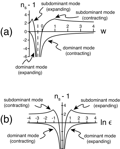
Since $\epsilon$ lies in the range $0\leq\epsilon<\infty$, this duality formally pairs every expanding ($\epsilon<1$) universe with a contracting ($\widehat{\epsilon}>1$) universe, and vice versa. However, the background solution (5) is only stable against small perturbations in two cases: (i) expanding with $\epsilon<1$ or (ii) contracting with $\epsilon>3$ PHZ_conditions ; chaos . Thus, an expanding model and its contracting dual are both stable when $\epsilon<1/3$ ($w<-7/9$) and $\widehat{\epsilon}>3$ ($\widehat{w}>1$). Also note, in agreement with PHZ_conditions , that there are only two limits in which an approximately scale-invariant ($n_{\textrm{grow}}-1\approx 0$) spectrum of scalar perturbations is produced: (i) when $\epsilon\rightarrow 0$ ($w\rightarrow-1$), corresponding to the inflationary regime and (ii) when $\epsilon\rightarrow\infty$ ($w\rightarrow\infty$) corresponding to the cyclic/ekpyrotic regime.

The dominant and subdominant pieces, $f_{{\rm dom}}(x)$ and $f_{{\rm sub}}(x)$ are related to the growing and decaying modes of $\bar{u}$ and $\bar{v}$, which may simply be obtained by replacing the Hankel functions in (21a,21b) with the corresponding Neumann functions or Bessel functions:

$$\bar{u}_{{\rm grow}}\propto x^{-1}Y_{\alpha}(x) \bar{u}_{{\rm decay}}\propto x^{-1}J_{\alpha}(x)$$ (32a)

$$\bar{v}_{{\rm grow}}\propto Y_{\beta}(x)\!\!\qquad \bar{v}_{{\rm decay}}\propto J_{\beta}(x).$$ (32b)

We may define growing-mode and decaying-mode spectral indices for $\bar{u}$ and $\bar{v}$, just as we did for $f_{{\rm sub}}$ and $f_{{\rm dom}}$ in (30). Now restrict attention to the ranges $\epsilon<1/3$ and $\widehat{\epsilon}>3$ (i.e. the range over which the duality pairs stable expanding models to stable contracting models). Then, using (32) along with the (24), we find

• The growing-mode and decaying-mode spectral indices associated with $\bar{u}$ are simply equal to $n_{{\rm dom}}$ and $n_{{\rm sub}}$, respectively.

• The growing-mode spectral index associated with $\bar{v}$ is equal to $n_{{\rm dom}}$ in an expanding ($\epsilon<1/3$) universe, but is equal to $n_{{\rm sub}}$ in a contracting ($\widehat{\epsilon}>3$) universe.

V Tensor perturbations

Tensor perturbations are much simpler than scalar perturbations. The perturbed metric is

$$\textrm{d}s^{2}/a^{2}=-\textrm{d}\tau^{2}+[\delta_{ij}+2h_{T}Y^{(2)}_{ij}]\textrm{d}x^{i}\textrm{d}x^{j}$$ (33)

where $Y^{(2)}_{ij}$ is a tensor harmonic (see Appendix C in Kodama_Sasaki ). The tensor perturbation $h_{T}$ is gauge-invariant and obeys

$$h_{T}^{\prime\prime}+2(a^{\prime}/a)h_{T}^{\prime}+k^{2}h_{T}=0.$$ (34)

It is useful to define a new variable $f_{T}\equiv ah_{T}$ which obeys

$$f_{T}^{\prime\prime}+(k^{2}-a^{\prime\prime}/a)f_{T}=0.$$ (35)

Again, the standard vacuum choice is the Minkowski vacuum of a comoving observer in the far past, corresponding to the boundary condition

$$f_{T}\rightarrow(2k)^{-1/2}e^{-ik\tau}\qquad\textrm{as}\quad\tau\rightarrow-\infty.$$ (36)

We can now solve for $f_{T}$, just as in the scalar case. But it is simpler to notice that (5) and (11) imply $z(\tau)\propto a(\tau)$, and hence $z^{\prime\prime}/z=a^{\prime\prime}/a$ when $\epsilon$ is constant. Thus, since $v$ and $f_{T}$ obey identical equations of motion (compare (12b) with (35)) and boundary conditions (compare (14b) with (36)), we find

$$f_{T}=v=\mathcal{P}_{2}(\pi x/4k)^{1/2}H_{\beta}^{(1)}(x).$$ (37)

The tensor spectral index is defined in the long-wavelength limit by $k^{3}|f_{T}|^{2}\propto k^{n_{T}}$. Using (24) and (37) we find

$$n_{T}=3-2\beta=3-\left|\frac{\epsilon-3}{\epsilon-1}\right|.$$ (38)

Note, in particular, that this expression is not invariant under $\epsilon\rightarrow 1/\epsilon$. An expanding universe with equation of state $\epsilon$ produces a tensor spectrum which is much redder than the tensor spectrum produced in a contracting universe with $\widehat{\epsilon}=1/\epsilon$: $n_{T}\leq\widehat{n}_{T}-2$.

VI Other dualities

It is interesting to contrast our duality with other cosmological dualities that have been discussed in the literature.

One duality, due to Wands Wands (see also Starobinsky ), pairs models that share the same “$v$” perturbations. By contrast, our duality pairs models that share the same “$u$” perturbations. (Note: the variable called “$u$” in Wands is called “$v$” in our paper, in agreement with Mukhanov’s convention pert_reviews ; Mukhanov .) Thus, whereas our duality connects expanding and contracting models through the substitution $\epsilon\rightarrow\widehat{\epsilon}=1/\epsilon$ (which leaves $\theta^{\prime\prime}/\theta$, and hence $u$, invariant), Wands’ duality instead uses the substitution $\epsilon\rightarrow\widehat{\epsilon}=(2\epsilon-3)/(\epsilon-2)$ (which leaves $z^{\prime\prime}/z$, and hence $v$, invariant). For example, his duality pairs an expanding inflationary solution ($\epsilon=0$, $w=-1$) with a contracting dustlike solution ($\widehat{\epsilon}=3/2$, $\widehat{w}=0$). Another difference between our duality and Wands’ stems from the fact that $v$ is purely subdominant (i.e. contains no dominant-mode contribution) in a contracting universe (see section IV). Thus, whereas our duality maps the expanding-phase dominant mode to the contracting-phase dominant mode, and the expanding-phase subdominant mode to the contracting-phase subdominant mode, Wands’ duality instead associates the expanding-phase dominant mode with the contracting-phase subdominant mode.

A second interesting duality, discussed by Brustein et al. Brustein , applies to a broad class of cosmological perturbations. Associated with each type of perturbation is a “pump”—a particular function of the background fields. The Hamiltonian governing a given perturbation is invariant under a transformation that swaps the perturbation with its conjugate momentum, and simultaneously inverts the appropriate pump function Brustein . It is instructive to apply this duality to the $u$ and $v$ variables considered in this paper. In this case, the Brustein et al. duality associates an expanding solution characterized by $\theta$ (or $\epsilon$) to a contracting universe characterized by $\widehat{\theta}=1/\theta=z$ (or $\widehat{\epsilon}=2-\epsilon$). The transformation $\epsilon\rightarrow\widehat{\epsilon}=2-\epsilon$ effectively swaps the variables $u$ and $v$

$$u\rightarrow\widehat{u}=(i/2k)v$$ (39a)

$$v\rightarrow\widehat{v}=(2k/i)u$$ (39b)

as may be verified from (19a,19b).

Recall that $\epsilon$ lies in the range $0\leq\epsilon<\infty$. Thus, our duality formally pairs every expanding ($0\leq\epsilon<1$) solution with a contracting ($1<\widehat{\epsilon}<\infty$) solution, and vice versa. By contrast, Wands’ duality relates every expanding solution to a contracting solution with $1<\widehat{\epsilon}\leq 3/2$; but contracting solutions with $\widehat{\epsilon}>3/2$ have no expanding dual. Similarly, Brustein et al.’s duality pairs every expanding solution with a contracting solution in the range $1<\widehat{\epsilon}\leq 2$; but contracting solutions with $\widehat{\epsilon}>2$ have no expanding dual.

The constant-$\epsilon$ background solutions (5) are only practically useful if they are dynamically stable. Recall that the contracting solutions are stable if and only if $\epsilon>3$ ($w>1$) PHZ_conditions ; chaos . Thus, Wands’ and Brustein et al.’s dualities relate every expanding solution to an unstable contracting solution. By contrast, our duality relates stable expanding solutions with $0\leq\epsilon<1/3$ ($-1\leq w<-7/9$) to stable contracting solutions with $3<\widehat{\epsilon}<\infty$ ($1<\widehat{w}<\infty$). In terms of the spectral index, this means that $n_{s}>0$ may be produced either by a stable expanding phase or by a stable contracting phase. In the real universe, the condition $n_{s}>0$ is satisfied (experiments favor $n_{s}\approx 1$), so that our duality is of practical relevance in cosmological model building. Some properties of the three different duality relations are summarized in Table I.

Transformation of		Range	Maps stable
background	perturbations	of $\epsilon$	to stable?	Ref.
$\epsilon\rightarrow 1/\epsilon\;\;\,$	$u\rightarrow u$	$[0,\infty)$	Yes, if $n_{s}>0$	-
$\epsilon\rightarrow\frac{2\epsilon-3}{\epsilon-2}\,$	$v\rightarrow v$	$[0,3/2]$	never	Wands ; Starobinsky
$\epsilon\rightarrow 2-\epsilon$	$u\leftrightarrow(i/2k)v$	$[0,2]$	never	Brustein

Table 1: Comparison of the duality presented here with those presented by Wands Wands ; Starobinsky and by Brustein et al. Brustein . The first two columns show how the background and perturbation variables transform under each duality. The third column shows the range of $\epsilon$ to which the duality applies. The fourth column indicates the condition under which an expanding background solution and its contracting dual are both stable under small perturbations.

Finally, a number of authors have discussed cosmological symmetries of the low-energy string effective action. If one neglects all fields in this action besides the dilaton and the metric, then there is a well–known “scale–factor duality” scalefacdual : starting with any cosmological solution, one can use this duality to generate new solutions. If, in addition to the dilaton, one includes other fields (axions, moduli,…), then the cosmological solutions may display more general dualities, and the resulting perturbation spectra may be invariant under these dualities stringdual . But note that these symmetries typically relate different solutions of a single effective action. By contrast, the dualities in Table I relate two different cosmological background solutions corresponding to two different Lagrangians: an expanding universe, with potential $V(\phi)$, is dual to a contracting universe, with a different potential $\widehat{V}(\phi)$.

VII Discussion

Beyond its inherent theoretical interest, our duality may be observationally relevant if (as discussed in section I) long-wavelength correlations produced during a contracting phase successfully propagate into a subsequent expanding phase. This suggests a fundamental degeneracy: an ideal measurement of the “primordial” scalar perturbation spectrum may be unable to determine whether the perturbations were generated by an expanding phase or by its contracting dual. Luckily, as shown in section V, tensor perturbations break this degeneracy: an expanding model produces a much redder tensor spectrum than its contracting dual. In particular, a detection of tensors in the cosmic microwave background would indicate that these perturbations were generated in an expanding phase, since the dual contracting phase would produce an undetectably small tensor spectrum on these cosmological length scales gravity_waves .

Using the background solutions (5), we may think of the duality as relating two different scale factors, $a(\tau)$ and $\widehat{a}(\tau)$, or two different scalar potentials, $V(\phi)$ and $\widehat{V}(\phi)$. Alternatively, recall that $a\propto|t|^{1/\epsilon}$ and $H^{-1}\equiv a^{2}/a^{\prime}\propto t$, where $t$ is the proper time of a comoving observer and $H^{-1}$ is the “Hubble scale.” Thus, two dual universes are related by

$$\textrm{d\,ln}H/\textrm{d\,ln}a=\textrm{d\,ln}\widehat{a}/\textrm{d\,ln}\widehat{H}.$$ (40)

So the duality effectively swaps the scale factor with the Hubble scale, and simultaneously swaps expansion and contraction. For example, in the $\epsilon\rightarrow 0$ ($w\rightarrow-1$) limit, the scale factor grows rapidly while the Hubble length grows slowly; whereas in the $\epsilon\rightarrow\infty$ ($w\rightarrow\infty$) limit, the Hubble length shrinks rapidly while the scale factor shrinks slowly. Expanding models in which modes exit the horizon most rapidly ($w\rightarrow-1$) and most slowly ($w\rightarrow-1/3$), are associated with contracting models in which modes exit most rapidly ($w\rightarrow\infty$) and most slowly ($w\rightarrow-1/3$), respectively.

Finally, let us mention several open questions. We have studied the duality using a simple model—spatially-flat FRW spacetime with a single scalar field $\phi$; what happens in more complicated models? We have used linear perturbation theory; what happens in the nonlinear regime? We have restricted ourselves to time-independent $\epsilon$; what if we allow time-varying $\epsilon$? This final question is treated in a companion paper dual2 .

*

Appendix A Generalization to arbitrary spacetime dimension

In sections II—V, we restricted our discussion to 4 spacetime dimensions. Here we sketch the generalization to $d$ spacetime dimensions, for $d\geq 4$. To understand this appendix, read sections II—V first. Gauge-invariant perturbation theory in $d$ spacetime dimensions is treated thoroughly in Kodama_Sasaki (see especially the appendices therein).

The background metric (1) obeys the Friedmann equations

$$(d-1)(d-2)a^{\prime\,2}\!/a^{4}=2\rho\qquad\qquad\qquad\qquad\;$$ (41a)

$$(d-1)(d-2)\,a^{\prime\prime}/a^{3}=(5-d)\rho-(d-1)p\quad$$ (41b)

where $\rho$ and $p$ are given by (3). Instead of $w\equiv p/\rho$, parameterize the equation of state with

$$\epsilon\equiv\frac{(2d-5)+(d-1)w}{d-2}.$$ (42)

From eqs. (3, 41) we find $-1\leq w<\infty$ or $\frac{d-4}{d-2}\leq\epsilon<\infty$. For constant $\epsilon$, the solution of (3, 41) is

$$\!\!\!\!\!\!\!\!\!\!\!\!\!\!\!\!\!\!\!\!a(\tau)=|\tau|^{2/[(d-2)(\epsilon-1)]}$$ (43a)

$$\!\!\!\!\!\!\!\!\!\!\!\!\!\!\!\!\!\!\!\!\phi_{0}(\tau)=\pm\frac{1}{\epsilon-1}\sqrt{2\left(\epsilon-\frac{d-4}{d-2}\right)}\;\textrm{ln}|\tau|$$ (43b)

$$\!\!\!\!\!\!\!\!\!\!\!\!\!\!\!\!\!\!\!\!V(\phi)=\frac{3-\epsilon}{(\epsilon-1)^{2}}\,\textrm{exp}\!\!\left[\mp\sqrt{2\left(\epsilon-\frac{d-4}{d-2}\right)}\;\phi\right]$$ (43c)

where we have chosen $a(0)=0$, $a(1)=1$ and $\phi_{0}(1)=0$.

As shown in Kodama_Sasaki , perturbations in $d$ spacetime dimensions may be decomposed into scalars, vectors and tensors, just as in 4 dimensions, and gauge-invariant variables may be defined. In particular, we can again introduce scalar perturbations through equations (6a, 6b), and describe these perturbations with a single gauge-invariant variable. The gauge-invariant Newtonian potential, $\Phi$, is most easily understood in “Newtonian gauge” ($B=H_{L}=0$), where it is related to the metric perturbations in a simple way: $\Phi=A=-(d-3)H_{L}$. The gauge-invariant variable $\zeta$ is most easily understood in “comoving gauge” ($H_{T}=\delta T^{0}_{i}=0$), where it is related to the spatial metric perturbation in a simple way: $\zeta=-H_{L}$. Note also that $\delta\phi=0$ in this gauge. If we take the $d$-dimensional definitions of $u$, $v$, $\theta$ and $z$ to be:

$$u\equiv\frac{1}{2}\left(\frac{d-2}{d-3}\right)\frac{a^{(d-2)/2}}{\phi_{0}^{\prime}}\Phi\qquad\qquad v\equiv z\zeta\\$$ (44)

$$\theta\equiv 1/z\equiv\frac{a^{\prime}}{a^{d/2}\phi_{0}^{\prime}},$$ (45)

then sections III and IV immediately generalize $d$ dimensions. Indeed, it is straightforward to show that equations (12) through (29) all remain true in $d$ dimensions, provided we take $\epsilon$, $u$, $v$, $\theta$, and $z$ to be given by their $d$-dimensional definitions (42), (44) and (45).

In particular, this means that the duality extends to $d$-dimensions: $u$, $f_{\textrm{grow}}$ and $f_{\textrm{decay}}$ are all invariant under $\epsilon\rightarrow 1/\epsilon$. The duality pairs expanding solutions in the range $\frac{d-4}{d-2}<\epsilon<1$ with contracting solutions in the range $1<\epsilon<\infty$. Note that for $d>4$, there are some contracting models with no expanding dual; but for $d=4$, every expanding model has a contracting dual, and vice versa.

In the $x\rightarrow 0$ limit in $d$ dimensions, define the growing and decaying spectral indices

$$x^{d-1}|f_{\textrm{grow}}|^{2} \propto x^{n_{\textrm{grow}}-1}$$ (46a)

$$x^{d-1}|f_{\textrm{decay}}|^{2} \propto x^{n_{\textrm{decay}}-1}.$$ (46b)

Then, using (17a), (24), (27), (28) and (29) we find

$$n_{\textrm{grow}}\;-1 = d-3-\;\Big{|}\frac{\epsilon+1}{\epsilon-1}\Big{|}$$ (47a)

$$n_{\textrm{decay}}-1 = d-1-\left|\Big{|}\frac{\epsilon+1}{\epsilon-1}\Big{|}-2\right|$$ (47b)

with $\epsilon$ given by (42). Note that these expressions are invariant under $\epsilon\rightarrow 1/\epsilon$.

As shown in Kodama_Sasaki , we may again introduce tensor perturbations through eq. (33). Now define the gauge-invariant variable $f_{T}^{(d)}\equiv a^{(d-2)/2}h_{T}$ which obeys

$$f_{T}^{\prime\prime}+[k^{2}-(a^{(d-2)/2})^{\prime\prime}/a^{(d-2)/2}]f_{T}=0$$ (48)

along with the boundary condition (36). Using (36), (43) and (48) we find that solution for $f_{T}$ is still given by (37) in $d$ dimensions. In the $k\rightarrow 0$ limit, define the tensor spectral index $k^{d-1}|f|^{2}\propto k^{n_{T}}$. Then, using (24) and (37) we find

$$n_{T}=d-1-\left|\frac{\epsilon-3}{\epsilon-1}\right|$$ (49)

with $\epsilon$ given by (42). Note that this expression is not invariant under $\epsilon\rightarrow 1/\epsilon$. This completes the generalization to $d$ spacetime dimensions.

References

- (1) A. H. Guth, Phys. Rev. D 23, 347 (1981); A. D. Linde, Phys. Lett. B 108, 389 (1982); A. Albrecht and P. J. Steinhardt, Phys. Rev. Lett. 48, 1220 (1982).
- (2) V. Mukhanov and G. Chibisov, Pisma Zh. Eksp. Teor. Fiz. 33, 549 (1981); A. H. Guth and S.-Y. Pi, Phys. Rev. Lett. 49, 1110 (1982); S. W. Hawking, Phys. Lett. B 115, 295 (1982); A. A. Starobinskii, Phys. Lett. B 117, 175 (1982); J. M. Bardeen, P. J. Steinhardt and M. S. Turner, Phys. Rev. D 28, 679 (1983).
- (3) J. Khoury, B. A. Ovrut, P. J. Steinhardt and N. Turok, Phys. Rev. D 64, 123522 (2001); J. Khoury, B. A. Ovrut, N. Seiberg, P. J. Steinhardt and N. Turok, Phys. Rev. D 65, 086007 (2002); P. J. Steinhardt and N. Turok, Science 296, 1436 (2002); P. J. Steinhardt and N. Turok, Phys. Rev. D 65, 126003 (2002).
- (4) J. Khoury, B. A. Ovrut, P. J. Steinhardt and N. Turok, Phys. Rev. D 66, 046005 (2002).
- (5) A. J. Tolley and N. Turok, Phys. Rev. D 66, 106005 (2002); A. J. Tolley, N. Turok and P. J. Steinhardt, hep-th/0306109.
- (6) S. Gratton, J. Khoury, P. J. Steinhardt and N. Turok, astro-ph/0301395.
- (7) J. Khoury, P. J. Steinhardt and N. Turok, Phys. Rev. Lett. 91, 161301 (2003).
- (8) L. A. Boyle, P. J. Steinhardt and N. Turok, to appear (2004).
- (9) R. Brandenberger and F. Finelli, JHEP 0111, 056 (2001); J. Martin, P. Peter, N. Pinto-Neto, D. J. Schwarz, Phys. Rev. D 65, 123513 (2002); 67, 028301 (2003); J. Martin and P. Peter, astro-ph/0312488.
- (10) T. J. Battefield, S. P. Patil, and R. Brandenberger, hep-th/0401010.
- (11) R. Kallosh, L. Kofman, and A. Linde, Phys. Rev. D 64, 123523 (2001); R. Kallosh, L. Kofman, A. Linde, and A. Tseytlin, Phys. Rev. D 64, 123524 (2001).
- (12) J. Khoury, B. A. Ovrut, P. J. Steinhardt, N. Turok, hep-th/0105212; see also http://feynman.princeton.edu/ steinh/cyclicFAQS.
- (13) G. T. Horowitz and J. Polchinski, Phys. Rev. D 66, 103512 (2002); H. Liu, G. Moore and N. Seiberg, JHEP 0206, 045 (2002); D. Lyth, Phys. Lett. B 524, 1 (2002).
- (14) J. K. Erickson, D. H. Wesley, P. J. Steinhardt and N. Turok, hep-th/0312009.
- (15) R. Durrer and F. Vernizzi, Phys. Rev. D 66, 083503 (2002); B. Craps and B. A. Ovrut, hep-th/0308057; C. Cartier, R. Durrer and E. J. Copeland, hep-th/0301198.
- (16) D. Wands, Phys. Rev. D 60, 023507 (1999).
- (17) A. A. Starobinsky, Pis’ma Zh. Eksp. Teor. Fiz. 30, 719 (JETP Lett. 30, 682) (1979).
- (18) R. Brustein, M. Gasperini and G. Veneziano, Phys. Lett. B 431, 277 (1998).
- (19) G. Veneziano, Phys. Lett. B 265, 287 (1991); A. Tseytlin, Mod. Phys. Lett. A 6, 1721 (1991); A. Sen, Phys. Lett. B 271, 295 (1991).
- (20) E. J. Copeland, R. Easther and D. Wands, Phys. Rev. D 56, 874 (1997); E. J. Copeland, J. E. Lidsey and D. Wands, Nucl. Phys. B 506, 407 (1997); J. E. Lidsey, D. Wands and E. J. Copeland, Phys. Rept. 337, 343 (2000); H. A. Bridgman and D. Wands, Phys. Rev. D 61, 123514 (2000); A. Buonanno, K. A. Meissner, C. Ungarelli and G. Veneziano, Phys. Rev. D 57, 2543 (1998); JHEP 9801, 004 (1998).
- (21) J. M. Bardeen, Phys. Rev. D 22, 1882 (1980).
- (22) H. Kodama and M. Sasaki, Prog. Theor. Phys. Suppl. 78, 1 (1984).
- (23) V. F. Mukhanov, H. A. Feldman and R. H. Brandenberger, Phys. Reports 215, 203 (1992).
- (24) V. F. Mukhanov, JETP Lett. 41, 493 (1985); Sov. Phys. JETP 68, 1297 (1988).
- (25) N. D. Birrell and P. C. W. Davies, Quantum Fields in Curved Space. Cambridge University Press, (1982).
- (26) J. Khoury, B. A. Ovrut, P. J. Steinhardt and N. Turok, Phys. Rev. D 64, 123522 (2001); L. A. Boyle, P. J. Steinhardt and N. Turok, hep-th/0307170.