1. Introduction

Observational cosmology has made tremendous progress over the last few years. Many of the traditional debates have now been settled, and we have converged on what seems to be a good phenomenological description of the observed universe. The universe is nearly flat, as expected from the simplest inflationary models[2], and the fluctuations seem to be primordial, Gaussian, linear, adiabatic and nearly scale-invariant, which was again the expectation from inflation[3]. Less comforting was the discovery that today’s universe possesses positive vacuum energy, a hundred orders of magnitude smaller than the vacuum energy needed to drive inflation. So any inflationary model not only needs the usual fine-tuning (at a level of $10^{-10}$ or so) required to produce density variations at the right level, but also needs fine-tuning of $10^{-100}$ or so to get today’s vacuum energy right.

The successes of inflation have helped people to forget its failures. Cosmology’s greatest conundrum, the initial singularity - the beginning of time and the origin of everything - remains as puzzling as ever. Proposals for avoiding an initial singularity, for example the no boundary proposal, do not seem successfully to predict the occurrence of inflation. In order to rescue the theory, some resort to anthropic arguments. However, it is questionable whether anthropic selection is really powerful enough to select a universe like ours.

Recently, it has been proposed that superstring theory vacua form a vast ‘discretuum’ within an immense landscape, and that inflation plus the anthropic principle may determine our observed vacuum. However, if we extrapolate back in time we always encounter the big bang singularity and the problem of how and why our region of the universe started out at some particular point on the landscape. These problems provide strong motivation for seeking an alternative to inflation, which deals with the cosmic singularity instead of assuming the universe started out just after it. Perhaps our failure to deal properly with the cosmic singularity is the source of the current unsatisfactory reliance upon ad hoc initial conditions. A more complete dynamical theory of the universe might yield physical attractor states to which the universe would be drawn so that we did not have to start it off ‘by hand’ in an arbitrary inflating state.

It seems to us that the time is right to try to do better. String theory and M theory encourage us to go beyond conventional field theory and gravity and to try and make sense of singularities. Within this framework, if consistent laws for passing through singularities can be uncovered, it seems entirely reasonable to expect that there was a universe before the singularity. Encouraged by the fact that the big bang singularity is much milder in brane world models, we have been developing an alternative to inflation. The basic idea is that the big bang was caused by the collision of two 3-branes colliding in a fourth spatial dimension. In the background solution, the 3-volumes of the branes remain finite at the collision even though this moment is the big bang singularity within the conventional Einstein gravity description.

The first version of our alternative scenario, called the Ekpyrotic universe[4], introduced a new mechanism for the production of scale-invariant adiabatic perturbations, in a pre-big bang epoch. The second version, the Cyclic universe[1], exploited the currently observed dark energy to solve the flatness and homogeneity puzzles, again before the big bang. This new cosmology provides a surprisingly complete picture of cosmic history in which high energy inflation is no longer required. Instead, the universe undergoes a periodic (and classically, eternal) sequence of big bangs and big crunches. Each bang results in baryogenesis, dark matter formation, nucleosynthesis and galaxy formation, and ends with an epoch of low energy acceleration of the type we see today. The decay of the dark energy generates both the energy required for the next big bang, and the scale-invariant density perturbations required for structure formation in the next cycle.

Unlike inflation, the cyclic model requires the presence of low energy acceleration, in order for the cycles to repeat. It offers the possibility of a physical (as opposed to anthropic) explanation for the value of today’s cosmological constant, with its incredibly small value in Planck units, as that required to sustain the attractor state. The cyclic attractor may also be involved in selecting the values of other presently unexplained constants including the baryon/dark matter/dark energy ratios.

The main challenge facing the cyclic scenario is that of tracking the state of the universe through the big crunch/big bang transition. As mentioned, the background density and curvature of the four-dimensional universe remain finite all the way to the singularity. However, the big crunch/big bang transition[5] is still singular because a fifth dimension (the gap between the branes) collapses to zero for a moment. The scenario is built upon the conjecture that this dimension immediately reappears, in a manner consistent with energy and momentum conservation suitably defined[1].

Can one define a consistent matching rule or S-matrix for fields and fluctuations across such singularities? As we discuss below, there is no problem in finding such a continuation for free quantum fields[6] and strings[24]. Recently, we extended this to linearised gravity, showing how scale invariant, adiabatic growing mode perturbations established before the singularity propagate into the hot big bang[7]. The resulting models yield an acceptable phenomenology for a broad range of parameters[8]. In fact, the perturbations in the cyclic and inflationary scenarios exhibit a surprising ‘duality’[10, 11], and the levels of tuning required to fit the observations are almost identical in the two models[9].

The challenge of extending the continuation across the singularity to nonlinear gravity remains. At the end of this review we review this problem, and why we are optimistic that it can be solved.

2. Brief Overview of the Cyclic Scenario

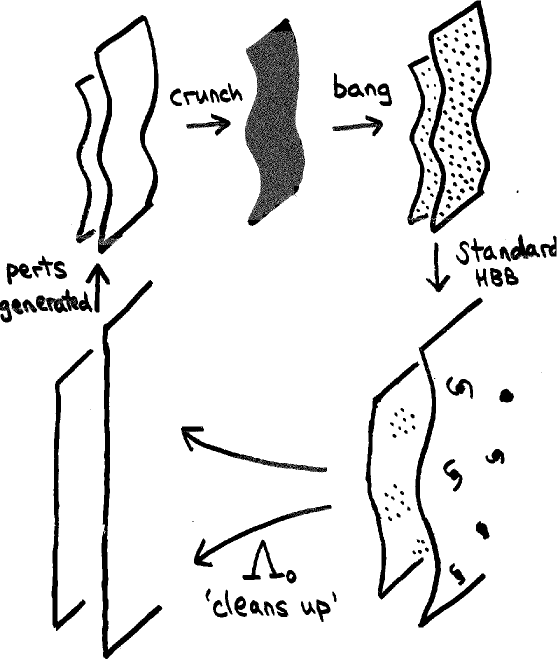
Figure 1: A cartoon showing cosmic evolution in the cyclic scenario.

A cartoon representation of the scenario is shown in Figure 1. We start with today’s universe on the lower right of the figure, assumed to consist of an M-theory setup with two parallel $Z_{2}$ branes separated by a small fifth dimension. Matter is confined to the branes - perhaps with baryonic matter on one, and the dark matter on the other. Positive vacuum energy causes the branes to expand exponentially in the noncompact directions, ‘cleaning up’ the universe by diluting away perturbations, galaxies, and other nonlinear structures to negligible levels. The flat homogeneous universe is a stable attractor and the horizon and flatness puzzles are solved much as they are in high energy inflation except over very much larger timescales - tens of billions of years. Following this low energy inflationary phase, the universe is restored to a ‘blank slate’ (lower left), ready for the imprinting of perturbations which will form galaxies in the next cycle.

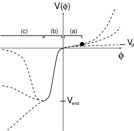
Figure 2: Scalar potentials suitable for a cyclic universe model. Running forward in cosmic time, Region (a) governs the decay of the vacuum energy, leading to the end of the slow acceleration epoch. Region (b) is the region where scale invariant perturbations are generated. In Region (c), as one approaches the big crunch ($\varphi\rightarrow-\infty$), the kinetic energy dominates.

Now, we assume that the two branes attract one another, with a force which decreases rapidly as the branes separate (Figure 2). Over cosmological timescales, the branes are slowly drawn together to eventually collide. The long wavelength physics may be described in four-dimensional terms, using a scalar field to represent the inter-brane separation. The potential for this scalar field is assumed to take the form shown in Figure 2. In this language, the positive vacuum energy phase is unstable because the scalar field slowly creeps downhill towards the region where the scalar potential steepens and becomes large and negative. As we show later, in a generic class of scalar potentials the scalar field acquires long wavelength, nearly scale-invariant perturbations as it runs downhill.

The two branes approach each other with increasing speed, and finally collide at a big crunch. In the background solution, the density and spacetime curvature of the branes are finite at the crunch even though there is a singularity when the fifth dimension disappears for an instant. When perturbations are present, the situation is more challenging. Generic four-dimensional perturbations, i.e. the low energy Kaluza-Klein modes, diverge logarithmically as one approaches the crunch, and a prescription such as analytic continuation is required in order to evolve them around $t=0$ and into the post-big bang universe. Such a continuation will be given below. The result is that the scale-invariant perturbations developed on the branes as they approach propagate into the hot big bang where they supply the adiabatic perturbations needed for concordance phenomenology.

Note that the cyclic model has a surprising economy. From the point-of-view of the four-dimensional effective field theory, one scalar field does everything: it provides today’s dark energy, it generates the density perturbations, regularises the singularity, and ignites the hot big bang. Furthermore, the five-dimensional view of the cyclic model even explains what the scalar field is - the size of an extra dimension - hence it arises naturally in string and M theory models.

Is the cyclic model observationally distinguishable from inflation? Gratifyingly, the answer is yes. High energy inflation produces a nearly scale-invariant spectrum of long wavelength gravitational waves as an inevitable side-effect. Because the cyclic universe does not involve high energy inflation, no such long wavelength waves are produced. In the simplest inflationary models - those with a single characteristic mass scale setting the shape of the effective potential during inflation – gravitational waves contribute substantially to the low multipole cosmic microwave anisotropy visible today, at the ten or twenty per cent level. Furthermore, they cause a distinctive ‘magnetic’ signal in the polarisation of the microwave sky, which may be measurable with the Planck satellite to be flown by ESA in 2007. If Planck detects magnetic polarisation, it will be a triumph for inflationary models and will rule out the cyclic alternative. Conversely, if Planck does not detect magnetic polarisation, it will rule out simple inflationary models.

3. Ekpyrotic Density Perturbation Mechanism

The ekpyrotic universe scenario[4] introduced a new mechanism for generating scale-invariant adiabatic perturbations during a contraction and bounce. The existence of such a simple alternative to the usual inflationary mechanism was a big surprise. At heart, the new mechanism is non-gravitational and the physics behind it can be understood by considering a four-dimensional scalar field $\varphi$ in Minkowski spacetime.

We consider a theory with a scalar potential which is flat at large $\varphi$ but which declines steeply as $\varphi$ decreases. A simple example is a negative exponential,

$$V(\varphi)=-V_{0}e^{-c\varphi},$$ (1)

with $V_{0}$ and $c$ positive constants. The initial conditions for the field are provided by the low-energy inflationary phase of the cyclic model, which leaves $\varphi$ near its Minkowski ground state but with a background value gently rolling downwards to negative values. Gravitational effects are subdominant since the potential and kinetic energies are both small. The background field $\varphi_{0}$ satisfies ${1\over 2}\dot{\varphi_{0}}^{2}+V(\varphi_{0})\approx 0$, which yields $\varphi\approx{2\over c}{\rm ln}(-At)$, with $A=c\sqrt{V_{0}/2}$. Here $t$ is negative and $t=0$ corresponds to $\varphi$ diverging. Fluctuations in $\varphi$ may be expanded as a Fourier series $\delta\varphi=\sum_{\vec{k}}\delta\varphi_{\vec{k}}e^{i\vec{k}\cdot\vec{x}}$. The field equation reads

$$\ddot{\delta\varphi}_{\vec{k}}=-\vec{k}^{2}\delta\varphi_{\vec{k}}-V_{,\varphi\varphi}\delta\varphi_{\vec{k}}+O(\delta\varphi^{2}),$$ (2)

in which the mass squared term $V_{,\varphi\varphi}=c^{2}V=-2/t^{2}$, from the above solution.

Those familiar with inflation will recognise the resulting equation

$$\ddot{\delta\varphi}_{\vec{k}}=-\vec{k}^{2}\delta\varphi_{\vec{k}}+{2\over t^{2}}\delta\varphi_{\vec{k}},$$ (3)

which describes the origin of scale-invariant perturbations in that context (although in inflation, $\delta\varphi$ is a conformally rescaled field and $t$ is the conformal time).

The initial conditions are that the positive frequency part of $\delta\varphi_{\vec{k}}$ is in its Minkowski vacuum

$$\delta\varphi_{\vec{k}}^{+}\sim{e^{-ikt}\over\sqrt{2k}},\qquad t\rightarrow-\infty,$$ (4)

where the $(2k)^{-{1\over 2}}$ factor is required by the usual canonical commutation relations. For early times, each Fourier mode oscillates under the influence of the $k^{2}$ term. However, when $|kt|$ becomes of order unity, the $2t^{-2}$ term in (3) starts to dominate, and the field mode evolution ‘freezes’ into a growing mode proportional to $t^{-1}$. Matching the two regimes, at $|kt|\sim 1$, we see that $\delta\varphi_{\vec{k}}\sim k^{-{3\over 2}}t^{-1}$ for $|kt|<<1$. The power spectrum is the square of this amplitude and is therefore proportional to $k^{-3}$. This is a scale invariant spectrum with equal power in each logarithmic interval of $k$.

In fact, the time-dependence of $\delta\varphi_{\vec{k}}$ may be seen to be just that of a local time delay in the background solution, $\varphi(t)=\varphi_{0}\left(t+\delta t(\vec{x})\right)$, or equivalently, a scale-invariant time delay to the big crunch. Including gravitational back-reaction (at the linearised level) in the four-dimensional effective theory has modest effect. While the perturbations are being generated, the gravitational fields are weak because the energy in the scalar field is small. And after the perturbations are generated, they are ‘frozen in’ as a time delay to the big crunch. Nevertheless, there is a slight reddening of the spectrum because the long wavelength perturbations are generated first, and have more time to self-gravitate[12]. The final result is expressible in similar terms to those usually used for slow-roll inflation: for a general potential of the required form, in the leading approximation including gravitational back-reaction, we obtain a scalar spectral index

$$n_{s}=1-4\left((V/V_{,\varphi})^{2}+(V/V_{,\varphi})_{,\varphi}\right).$$ (5)

Here, as in inflation, the right hand side is to be evaluated as the Fourier modes concerned freeze out, when $|kt|$ becomes smaller than unity. (Here and below we employ units in which $8\pi G$ is unity).

In inflation, departures from scale invariance are described by ‘slow-roll’ parameters, dimensionless measures of the first and second derivatives of the potential $V(\varphi$). In the cyclic model one finds deviations from scale invariance are similarly controlled by ‘fast-roll’ parameters that measure the steepness of the potentials[10]. The amount of tuning required to obtain consistency with the observations is nearly the same in both cases[9]. A simple example of a working potential is the form (1), for which $n_{s}-1=4/c^{2}$, so that $c>10$ is required to obtain a scalar spectral index $n_{s}>0.96$, compatible with the WMAP data [13].

Can we get through the singularity?

In order for the scale-invariant perturbations generated in the pre-big bang epoch to be useful in today’s universe, we have to be able to track them across the singularity. Whether we can do this consistently is the key challenge to the cyclic scenario, and most of the rest of this review will be devoted to it.

Compactified Milne mod $Z_{2}$

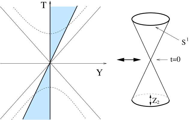
Figure 4: Orbifold construction of a big crunch big bang spacetime. One considers an embedding Minkowski spacetime, and then identifies the upper and lower wedges (the Milne universe) under discrete boosts. This produces the ‘double-cone’ at the right. Under a further $Z_{2}$ identification, one produces a spacetime with two boundary branes approaching, colliding at $t=0$ and re-emerging.

In the cyclic scenario, the singularity occurs when the two boundary branes collide and the fifth dimension momentarily disappears. The two branes have nonzero tensions (one positive and the other negative) and the bulk spacetime has a corresponding warp. However, in the background solution, which possesses cosmological symmetry, a Birkhoff-like theorem applies, and coordinates may be chosen in which the bulk is static. That is, if one sits in between the branes, there is no indication that the branes are coming until they actually arrive. Therefore, in between the branes, one can choose locally Minkowski coordinates. In fact, as $t=0$ approaches the branes behave to leading order as $Z_{2}$ reflection planes in Minkowski spacetime (Figure 4).

A model of the collision is provided by Minkowski spacetime modded out by discrete boosts, and then by an orbifold $Z_{2}$ projection. Consider five-dimensional Minkowski spacetime with the line element

$$ds^{2}=-dT^{2}+dY^{2}+d\vec{x}^{2}=-dt^{2}+t^{2}dy^{2}+d\vec{x}^{2},$$ (6)

where $T=t\cosh y$ and $Y=t\sinh y$. The coordinates $(t,y)$ cover the causal past and future of the origin. We call this half of Minkowski spacetime the Milne universe. We can further identify the spacetime under discrete boosts by identifying $y$ with $y+L$, compactifying the $y$ coordinate and producing the ‘double-cone’ shown on the right of Figure 4, which we call compactified Milne spacetime. Finally, we impose the $Z_{2}$ symmetry by identifying $y\leftrightarrow L-y$ so that the branes are now the edges of the cone shown converging for $t<0$, meeting at $t=0$ and emerging with the same relative speed at $t>0$. We call the resulting spacetime Compactified Milne mod $Z_{2}$ or ${\cal M}^{C}/Z_{2}$, and it is the model spacetime for which we develop a matching rule. We will see that this rule the forms the basis for analysing more general and realistic cosmological models.

Free Fields

Classically, the evolution of fields on ${\cal M}^{C}/Z_{2}$ is ill-defined for obvious reasons. There is no Cauchy surface at $t=0$, so fields cannot be propagated across that point. However, such a viewpoint is certainly too naive. We are not interested in observing the fields at $t=0$. Rather, we seek to construct a satisfactory S-matrix relating the possible ‘in’ and ‘out’ states. There are at least three separate ways of doing so, each of which leads to the same result [6]:

(i) Summing boosted copies of Minkowski plane waves. One can construct a complete basis for ${\cal M}^{C}/Z_{2}$ by summing standard Minkowski plane waves over boosts $y\rightarrow y+nL$, for integer $n$, and projecting onto $Z_{2}$-invariant modes[6]. The basis so derived is defined globally and hence yields a unique propagation rule across $t=0$.

(ii) Analytic continuation. This is the most powerful method since it extends to nonlinear fields, but it is also the least intuitive. The equation of motion for the Fourier modes of a free fields on ${\cal M}^{C}/Z_{2}$ is

$$\ddot{\varphi}+{1\over t}\dot{\varphi}=-k^{2}\varphi-{k_{y}^{2}\over t^{2}}\varphi.$$ (7)

One has to continue the solutions around the singularity at $t=0$. The equation is just Bessel’s equation and the incoming positive (negative) frequency modes of (7) are analytic in the lower half (upper half) complex $t-$ plane. The natural continuation of each is below or above $t=0$ respectively. (This is the standard analytic continuation for Hankel functions from positive to negative argument).

(iii) Decomposition into left and right movers, and real propagation in the embedding spacetime ‘around’ the singularity. Any solution of (7), when evolved towards $t=0$, splits into a sum of left and right moving modes. The left movers are regular on the left lower light cone $Y=T<0$; the right movers on the right lower light cone $Y=-T>0$. The left/right movers therefore have a well defined continuation into the left and right wedges of Minkowski spacetime. A natural assumption is that no other data enters these regions from past null infinity. Since the $k^{2}$ term in (7) behaves like a mass, the left/right movers eventually propagate into the future light cone, providing a unique propagation rule across $t=0$.

These three prescriptions turn out to yield the same matching rule across $t=0$, which furthermore maps the incoming adiabatic vacuum defined as $t\rightarrow-\infty$ to the outgoing adiabatic vacuum defined as $t\rightarrow+\infty$. Therefore for free fields there is no particle production. The $k_{y}=0$ modes behave as

$$\varphi_{\vec{k}}\sim Q+P{\rm ln}|kt|,\quad|t|\rightarrow 0,$$ (8)

and the continuation rules (i), (ii) or (iii) yield

$$P_{out}=P_{in}\qquad Q_{out}=-Q_{in}+2(\gamma-{\rm ln}2)P_{in},$$ (9)

where $P_{in}$, $P_{out}$ and $Q_{in}$, $Q_{out}$ are the constants appropriate to the incoming ($t<0$) and outgoing ($t>0$) field. This result is not time reversal at the bounce, $P_{out}=P_{in}$, $Q_{out}=Q_{in}$, which would produce the time-reversed universe coming out.

Picture (iii) provides helpful insight into the result (9). To the left mover entering the left wedge of Minkowski, one must add a right moving wave, with opposite sign, in order to ensure the field vanishes at infinity. This right mover then enters the future light cone leading to the sign reversal in $Q$. This sign change is universal and insensitive to the warp factor and the long time behaviour of the system far from the collision[7]. The second term involving the Euler constant is specific to the embedding Minkowski spacetime and would change if we included the effect of the warping and cosmological evolution. Happily, in the cosmological perturbation problem, $P_{in}$ is of order $k^{2}$ times $Q_{in}$ and hence negligible on large scales (small $k$). The sign flip of $Q$ turns out to be the key to the propagation of large scale growing mode perturbations across the singularity.

Cosmological Perturbations

In a recent paper[7], we have analysed the propagation of perturbations across a big crunch/big bang collision between two boundary branes, including general relativity at a linearised level. The question of choosing a gauge is especially subtle in singular spacetimes, since well-defined transition functions do not exist across the singularity. How do you then compare what comes in with what goes out? One requires a common coordinate system linking two Cauchy surfaces in the incoming and outgoing spacetimes.

Our procedure is to choose coordinates (or gauge) in which each of the incoming and outgoing spacetimes tend asymptotically, as $t$ tends to zero, to perturbed ${\cal M}^{C}/Z_{2}$ in a particular gauge-fixed gauge, in which the gravitational perturbations evolve as massless fields on ${\cal M}^{C}/Z_{2}$. The rules defined above tell us how to match such fields across $t=0$ in the model spacetime. For $t>0$, the perturbations on ${\cal M}^{C}/Z_{2}$ in our chosen gauge are in one-to-one correspondence with perturbations in the real spacetime and we use this correspondence to map them onto the outgoing state.

In ${\cal M}^{C}/Z_{2}$, the modes of interest are just those of five-dimensional linearised gravity. The $k_{y}=0$ modes of the five massless gravitons provide the four-dimensional massless fields. Two yield four-dimensional gravitons. Two more give a four-dimensional gauge potential, but the $Z_{2}$ projection removes this. The remaining mode is a four-dimensional scalar perturbation. This last mode is the one which is crucial for cosmological density perturbations.

We need to choose a gauge in which we can treat the full, warped spacetime, and easily relate it to the model spacetime in which the analysis is much simpler. Much of the work of Ref. References was to find such a gauge and show that the matching was uniquely defined within it. In this gauge, the four-dimensional scalar mode is represented as

$$ds^{2}=(1+{4\over 3}k^{2}\chi)(-dt^{2}+t^{2}dy^{2})+\left[(1-{2\over 3}k^{2}\chi)\delta_{ij}+2k_{i}k_{j}\chi\right]dx^{i}dx^{j},$$ (10)

and the field $\chi$ obeys the five dimensional massless equation $\nabla^{2}\chi=0$, with Neumann boundary conditions on the branes, $\partial_{y}\chi|_{y_{\pm}}=0$ (following from the $Z_{2}$ symmetry). Since $\chi$ is a free field in compactified Milne mod $Z_{2}$, we are able to apply the matching rule (8) across $t=0$.

So much for the model spacetime. To treat the actual spacetime, we need to include the effect of the warped bulk. We study a Randall-Sundrum model of type I with a positive and negative tension brane separated by a negative $\Lambda$ bulk. We choose a coordinate system in which the branes are at fixed $y=y_{\pm}$. The full metric, including linearised scalar perturbations, is

$$ds^{2}=n^{2}(t,y)\left(-(1+2\Phi)dt^{2}-2Wdtdy+t^{2}(1-2\Gamma)dy^{2}\right)+b^{2}(t,y)\left((1-2\Psi)\delta_{ij}-2\nabla_{i}\nabla_{j}\chi\right)dx^{i}dx^{j}.$$ (11)

For the background, we use the known solution in static coordinates (Schwarzschild-AdS). We can perform a coordinate transformation to a system in which the branes are fixed (i.e. $y=y_{\pm}$) as a Taylor expansion in $t$ around $t=0$. For the perturbations, we choose a gauge where $\Gamma=\Phi-\Psi-k^{2}\chi$. In this gauge, it turns out that the $\chi$ perturbation obeys $\nabla^{2}\chi=0$ (in the full five-dimensional metric), just as it did in the model ${\cal M}^{C}/Z_{2}$ spacetime. Furthermore, there is just enough residual gauge freedom to ensure that, as $t$ tends to zero, the perturbed metric agrees with the perturbed model spacetime (10) in which the matching of free gravitational waves is trivial.

In the vicinity of the singularity, we solve for the background and the perturbations as a series in $t$ and ln$|kt|$, around $t=0$. The four-dimensional effective theory is used to provide the boundary data; i.e. the spacetime metrics on the two branes. From the five dimensional Einstein equations, we obtain Schrodinger-like equations in $y$ at each order in $t$, $t$ln $|kt|$, $t^{2}$, $t^{2}$ln$|kt|$, $\dots$, which may be solved at each order by imposing the boundary conditions appropriate to the gauge choice made. We have checked that we obtain in this way a consistent solution of five dimensional linearised general relativity up to order $t^{3}$. There is precisely enough residual gauge freedom to choose the metric perturbations defined by (11) so that they take at leading order the form (10) corresponding to the model spacetime i.e.

$$W = 0+O(t,{\rm ln}|kt)$$ (12)

$$\Phi = {2\over 3}k^{2}\chi+O(t,t{\rm ln}|kt)$$ (13)

$$\Psi = {1\over 3}k^{2}\chi+O(t,t{\rm ln}|kt)$$ (14)

$${\chi^{\prime}\over nt}(y_{\pm}) = 0+O(t,{\rm ln}|kt),$$ (15)

as $t$ tends to zero. This new gauge is now completely fixed, to leading order in $t$. Therefore, by applying the rule determined for free fields in compactified Milne mod $Z_{2}$, we obtain a unique matching rule from the incoming fields to the model spacetime and from the model spacetime to the outgoing fields.

Boundary Conditions: 4d Effective Theory

Obtaining a matching rule in the five dimensional theory is only half of the story. To solve the full problem, one has to follow the perturbations from their generation well before the singularity, until they reach their asymptotic behaviour as $t\rightarrow 0$ in the big crunch. And after matching across $t=0$, one must solve for their evolution all the way into the late universe where we are interested in their observational effects.

All of the work of evolving to and from $t=0$ is done by a very powerful technique, employing a four-dimensional effective theory in the place of the full five dimensional one. This changes the difficulty of the problem from one of solving PDEs in $t$ and $y$ to ODEs in $t$ alone, a far easier task. In our recent work[7], we gave a new and simpler derivation of the four-dimensional effective theory, that shows how it reproduces the exact solutions for moving empty branes with cosmological symmetry. When matter is present on the branes, the four-dimensional theory is still correct up to $\rho^{2}$ terms which are consistently small at all times in the cyclic scenario.

The four-dimensional theory is used to predict the geometries of the positive and negative tension branes, thus providing the boundary conditions for the five dimensional equations as $|t|\rightarrow 0$. The four-dimensional effective theory is Einstein gravity plus a minimally-coupled scalar field $\varphi$ representing the inter-brane separation. The spacetime metrics $g_{\mu\nu}^{\pm}$ on the positive and negative tension branes are then given by[7]:

$$g_{\mu\nu}^{+}={\rm cosh}^{2}(\varphi/\sqrt{6})g_{\mu\nu}\qquad g_{\mu\nu}^{-}={\rm sinh}^{2}(\varphi/\sqrt{6})g_{\mu\nu},$$ (16)

where $g_{\mu\nu}$ is the Einstein frame metric in the 4d theory and we use units in which $8\pi G=1$. Near the brane collision, the four-dimensional effective theory becomes singular: the Einstein frame scale factor tends to zero as $t^{1\over 2}$ where $t$ is the conformal time, and the scalar field tends to minus infinity, $\varphi\sim\sqrt{3/2}{\rm ln}|t|$, so that both brane metrics are well behaved as $t$ tends to zero.

In the four-dimensional effective theory, the scale-invariant cosmological perturbations are generated by the potential shown in Figure 2. For $t<0$, the scale factor in the four-dimensional effective theory is contracting, and, as $t$ approaches zero, the perturbations in the growing mode freeze out. The four-dimensional Einstein frame metric is, in conformal Newtonian gauge,

$$ds^{2}_{(4)}=a^{2}(t)\left(-(1+2\Phi)dt^{2}+(1-2\Psi)d\vec{x}^{2}\right),$$ (17)

with $\Phi=\Psi$ since there are no anisotropic stresses to linear order. The equations describing the perturbations as $t\rightarrow 0$ are:

$$\delta\varphi^{\prime\prime}+2{\cal H}\varphi^{\prime} = -k^{2}\varphi+4\varphi^{\prime}\Phi,$$ (18)

$$\Phi^{\prime}+{\cal H}\Phi = {1\over 2}\varphi^{\prime}\delta\varphi,$$ (19)

where primes denote conformal time derivatives and ${\cal H}=a^{\prime}/a$. It is convenient to parameterise the solution in terms of the behaviour of the comoving energy density perturbation, $\epsilon=-{2\over 3}{\cal H}^{-2}k^{2}\Phi$, which has the following asymptotic behaviour:

$$\epsilon\sim\epsilon_{0}\left(1-{1\over 2}k^{2}t^{2}{\rm ln}|kt|+\dots\right)+\epsilon_{2}\left(t^{2}+\dots\right),$$ (20)

and the two constants $\epsilon_{0}$ and $\epsilon_{2}$ define the solution for the other variables:

$$\Phi = \epsilon_{0}\left(-{3\over 8k^{2}t^{2}}+{3\over 16}{\rm ln}|kt|+\dots\right)-\epsilon_{2}\left({3\over 8k^{2}}+\dots\right),$$ (21)

$$\varphi = \epsilon_{0}\left({3\over 8k^{2}t^{2}}+{1\over 16}{\rm ln}|kt|+{1\over 8}+\dots\right)-\epsilon_{2}\left({1\over 8k^{2}}+\dots\right),$$ (22)

$$\zeta_{M} = \epsilon_{0}\left(+{1\over 4}{\rm ln}|kt|+{1\over 8}+\dots\right)-\epsilon_{2}\left({1\over 2k^{2}}+\dots\right),$$ (23)

where we have also given the expression for $\zeta_{M}$, which is the curvature perturbation on comoving (or constant $\varphi$) slices. Note that conformal Newtonian gauge is very convenient for the analysis of the generation of the perturbations, and also for relating the four- and five-dimensional theories since it is completely gauge fixed. A further advantage is that one can straightforwardly read off the five dimensional $\Phi$ and $\Psi$ perturbations on the branes from the four-dimensional $\Phi$, $\Psi$ and $\delta\varphi$ perturbations, according to the formulas given in (16). However, the Newtonian gauge perturbations are badly divergent, as $t^{-2}$, and do not behave as free fields in compactified Milne. Hence it is essential to transform into a better behaved gauge such as (15) in order to match perturbation variables across $t=0$.

Examining equations (23), note that $\epsilon_{0}$ parameterises the the growing mode in the incoming state. In conformal Newtonian gauge, both the scalar field and gravitational potential possess nearly scale-invariant perturbations i.e. $\epsilon_{0}/k^{2}$ has a nearly scale-invariant spectrum. Conversely, $\epsilon_{2}$ is the amplitude of the decaying mode, and this is negligible on long wavelengths. The curvature perturbation on $\delta\varphi=0$ slices, $\zeta_{M}$, has no long wavelength power.

Previous treatments of cosmological perturbations in singular spacetimes, for example in the pre-big bang scenario[23], have for the most part simply assumed that at long wavelengths, $\zeta_{M}$ should be matched across the singularity. In our work, we developed an ab initio matching rule based on quantum field theory in a model spacetime which is the asymptotic limit of the real situation. Our finding is that, with this more sophisticated and cutoff-independent procedure, one does not, in general, obtain matching of $\zeta_{M}$ at long wavelengths.

The reason is easy to understand. When we match modes from $t<0$ to $t>0$, we should remember that, in general, we are matching them from two unrelated coordinate systems. It is essential to choose coordinate systems on either side so that the $t=0^{-}$ and $t=0^{+}$ time slices physically coincide(see Figure 5): otherwise it makes no sense to match perturbations on them. The only common timeslice is the brane collision slice: therefore one must choose coordinate systems for $t<0$ and for $t>0$ in which the the collision event is simultaneous. What our five-dimensional calculations reveal is that the brane collision is not simultaneous on $\delta\varphi=0$ slices, but it is in our matching gauge defined above.

The $\delta\varphi=0$ slices are natural from the four-dimensional effective theory point of view because the scalar field provides a natural time slicing of the spacetime. However, in the five dimensional picture, $\varphi$ only describes the brane separation for static branes. When the branes are moving, there are corrections to the distance relation depending on the brane speed and the bulk curvature. Roughly speaking, the gauge choice $\delta\varphi=0$ ensures no velocity perturbations tangent to the branes whereas collision simultaneity requires no velocity perturbations normal to the branes. The gauge transformation required to go from $\delta\varphi=0$ gauge to our gauge is scale-invariant in form, and introduces a scale-invariant curvature perturbation on the collision surface. Thus, in a collision-simultaneous gauge the spatial metrics on the branes acquire long wavelength, near-scale invariant curvature perturbations at the collision.

Finally, let us mention some recent work confirming aspects of the above analysis. Craps and Ovrut [24] have analysed a string theory $SL(2,R)/U(1)$ model which possesses a singularity which is locally of the same type as ${\cal M}^{C}/Z_{2}$. Through a group-theoretic analysis they determine a matching rule which is fully consistent with ours in the limit of high momenta. A recent analysis by Battefield et al. [25] including gravitational back-reaction in the same brane model we use has confirmed our result for $\zeta_{M}$ although, unlike us, they prefer to simply ignore the logarithmically divergent modes.

The result for the long wavelength curvature perturbation amplitude in the four-dimensional effective theory, propagated into the hot big bang after the brane collision is:

$$\zeta_{M}={9\epsilon_{0}\over 16k^{2}L^{2}}{\tanh(\theta/2)\over\cosh^{2}(\theta/2)}(\theta-\sinh\theta)\approx-{3\epsilon_{0}V_{coll}^{4}\over 64k^{2}L^{2}}$$ (24)

where $\theta$ is the rapidity corresponding to the relative speed $V_{coll}$ of the branes at collision, and the second formula assumes $V_{coll}$ is small. $L$ is the bulk curvature scale, and as we saw above, $\epsilon_{0}\over 16k^{2}$ has a scale-invariant power spectrum. The presence of radiation on the branes before or after the collision produces an additional correction term given in full in Ref. References. As discussed above, the physical origin of the curvature perturbation is in the time delay between the collision timeslice and the $\delta\varphi=0$ (or comoving) hypersurfaces, on which the branes do not possess long wavelength scale invariant curvature perturbations.

The nonlinear regime

We have developed and successfully implemented a natural prescription for matching free fields and linear cosmological perturbations across singularities of the type involved in the cyclic and ekpyrotic scenarios. However, the story is far from complete because we have not yet included nonlinear effects. In the gauge we use, perturbations remain small until times exponentially smaller than the Planck time, but nevertheless they generically diverge at $t=0$ meaning that nonlinear effects become important. We need a fully nonlinear matching rule to deal with these.

One useful viewpoint is provided by the standard Kaluza Klein reduction which gives the four-dimensional Newton constant in terms of the five-dimensional Newton constant divided by the size of the fifth dimension. As the latter disappears, we are inexorably led into the regime of strong gravity.

This effect is present in our linearised calculations. Even in the least divergent gauges, perturbations diverge logarithmically in time as $|t|\rightarrow 0$. The logarithmic divergence is not a four-dimensional gauge artifact, as is easily seen[12]. Tensor perturbations, which are gauge-invariant in linear theory, behave as free fields on a Milne spacetime and tend to $Q+P{\rm ln}|kt|$ as $|t|\rightarrow 0$. For scalar perturbations, one has only to see that the perturbation to the four-dimensional Ricci scalar diverges to reach the same conclusion (for another argument see [19]).

As nonlinearities become large, one should anticipate that perturbation theory will break down. This does not mean that a big crunch/big bang transition is impossible. In this section we want to explain why we believe there are grounds for optimism.

First, let us study the log divergence in more detail. Consider a $y$-independent tensor mode propagating in compactified Milne (6) in the $3$ direction. Assume the diagonal mode for simplicity: $h_{11}=-h_{22}$, with all other components zero. The equation of motion is:

$$\ddot{h}_{11}+{1\over t}\dot{h}_{11}=-k_{3}^{2}h_{11},$$ (25)

leading to the familiar behaviour $h_{11}=Q+P{\rm ln}|kt|$ as $|t|\rightarrow 0$. It is not hard to see where this linearised behaviour leads in the nonlinear theory. The $k$ dependence may be absorbed into $Q$ and $P$ and, after Fourier transforming back to real space, one sees that the spatial dependence factorises. Kasner solutions are given (in any dimensions) by

$$ds^{2}=-dt^{2}+\sum_{i}A_{i}t^{2p_{i}}dx_{i}^{2},$$ (26)

where $\sum_{i}p_{i}=\sum_{i}p_{i}^{2}=1$ and the $A_{i}$ are constants. The background compactified Milne solution is $p_{5}=1$, $p_{1}=p_{2}=p_{3}=0$. A small perturbation may be produced by setting $p_{1}=\epsilon<<1$ and $p_{2}=-\epsilon$, and the other $p$’s are unperturbed. This solves the Einstein equations to order $\epsilon$. To leading order in $\epsilon$, the exact asymptotic solution for the metric components takes the form $|t|^{\epsilon}\approx(1+\epsilon{\rm ln}|t|)$, and we recover the time dependence of the linearised gravitational wave above.

Even though the theory is becoming nonlinear, there is compensating simplicity near $t=0$ due to the phenomenon of ultralocality. As we approach the big crunch (or the big bang), long wavelength modes cease to be dynamical. There is just not enough time for them to move. To cosmologists this is familiar as the freezeout mechanism occurring when modes leave the Hubble horizon. In the present context, the Hubble horizon is proportional to $t$, so all modes freeze out on the way to $t=0$. It is known that (in the non-chaotic case - see below) a generic solution of the Einstein equations tends asymptotically to the Kasner form but with $A_{i}$ and $p_{i}$ being local functions of $\vec{x}$. From this asymptotic solution, we can now see exactly how perturbation theory breaks down. In the ultralocal limit, the exact solutions involve metric components behaving like $A(x)t^{\epsilon}(x)=A(x)\left(1+\epsilon(x){\rm ln}t+{1\over 2}(\epsilon(x){\rm ln}t)^{2}+..\right)$. Clearly, for small enough $t$, the higher orders dominate and the perturbative expansion in $\epsilon$ fails.

String theory calculations[18] reveal that naive string perturbation theory breaks down in singular spacetimes like compactified Milne mod $Z_{2}$. This breakdown may be a reflection of a poor choice of variables i.e., representing the perturbed metric as $g_{\mu\nu}^{(0)}+h_{\mu\nu}$ and expanding in $h_{\mu\nu}$. As we have just seen, higher order terms are crucial in representing the Kasner solution. It seems likely to us that perturbation theory needs to be re-summed to incorporate the effect of the changing background as $t$ tends to zero. A trivial example is provided by a scalar field with an action $\int dt|t|\left(\dot{h}^{2}-(\nabla h)^{2}\right)(1+h)$. At linear order, this theory has the same $Q+P{\rm ln}|kt|$ behaviour we have been discussing. At next order, one sees that the energy density in the field provides a diverging source term in the field equations: $\ddot{h}+t^{-1}\dot{h}+k^{2}h\sim\dot{h}^{2}$. This causes the breakdown of first order perturbation theory. However, a simple field redefinition $dH=(1+h)^{1\over 2}dh$ removes the interaction and results in a free field of exactly the type we have been discussing. Of course, gravity is far more complicated than this, but the example is indicative. The failure of first order perturbation theory should not be interpreted to mean that no continuation is possible in the nonlinear theory.

Horowitz and Polchinski[17] have claimed that the breakdown of string perturbation theory signals a disastrous instability. Even accepting that a bounce is possible in an ideal background compactified Milne universe, they argue that the introduction of a single particle would cause the entire space-time to collapse into a giant black hole. We believe this picture is misleading and that the true story is consistent (modulo the issue of chaos, see below) with the locally-Kasner picture we have advocated for some time. Let us examine this claim within linear theory, extrapolated as ultralocal Kasner evolution as $t$ approaches zero. If we introduce into compactified Milne a point particle (or more accurately a line density uniform in the fifth dimension but localised in the noncompact directions) of mass $m$, one can easily show using orbifold techniques that it cannot not alter the spacetime geometry outside of its future light cone[20], as one would intuitively guess. If the particle has existed for an arbitrarily long time, it alters the metric at arbitrary distances, but only by a small amount. And this metric perturbation evolves into locally Kasner evolution as one approaches the singularity, just as one would expect in the generic case. The near field of the particle yields a Newtonian potential $\Phi\sim-G_{4}m/r\sim-r_{0}^{2}/(rt)$, with $r_{0}$ a constant, because the four-dimensional Newton constant is proportional to $t^{-1}$. The far field is more interesting - at a separation $r$ from the particle, modes freeze out (and cease to be sourced by the particle) at a time $|t|\sim r$. Thereafter, these perturbations grow logarithmically in time up to $t=0$, yielding a far field metric perturbation of the form $\sim(r_{0}^{2}/r^{2}){\rm ln}(r/|t|)$. The ultralocal Kasner picture tells us precisely how this extrapolates to the singularity. The deformation of the spacetime induced by the particle changes the original compactified Milne singularity into a more generic Kasner singularity. It does so ultralocally, and in a way which has nothing to do with with the formation of an event horizon or a trapped surface.

Even though the evolution of the metric becomes ultralocal, another complication arises on the way to the singularity. Namely, gravitational theories can possess a chaotic, anisotropic, Mixmaster behaviour as $t$ tends to zero. At first sight, this would seem to be highly problematic for any putative matching rule, since there is no simple asymptotic behaviour on either side of the singularity. However, in recent work[21], we have pointed out that in our context the problem is less severe than one might have expected. It turns out that the potential which we require to generate perturbations has the unexpected effect of suppressing anisotropies, and hence chaos, because it produces an equation of state $w=P/\rho>>1$. The scalar field energy blueshifts far more quickly than anisotropic curvature and hence prevents the Mixmaster effect. If the interbrane potential is bounded below, then eventually the scalar field kinetic energy comes to dominate. In this situation, it is known that all string theories are borderline chaotic at leading order in $\alpha^{\prime}$. That is, the coupling of the dilaton to gauge fields is precisely the value below which chaos ceases to exist.

To summarise, the theory is under excellent perturbative control all the way to one string time before the singularity. First, the initial perturbations are small. Second, the incoming state is steered away from chaos by the $w>>1$ equation of state. Finally, as $t\rightarrow 0$, we are within a theory which is only marginally chaotic. One can safely conclude that there is no chaos up to one string time before $t=0$. More we cannot say, until we possess a better understanding of the $\alpha^{\prime}$ corrections.

In the analytic continuation procedure outlined above, it may be possible to avoid $t=0$ in the complex $t-$plane by analytically continuing around the singularity from negative to positive real values of $t$ in a semicircle with radius greater than the string scale. Then, the calculation given above would remain essentially uncorrected by nonlinear gravitational effects, at least on long (three-dimensional) wavelengths. Work is currently in progress to construct such a continuation in nonlinear gravity.

Another intriguing connection hinting at hidden simplicity in singularity behaviour is provided by a recent analysis of the classic Belinskii-Khalatnikov-Lifshitz analysis of cosmological singularities in the context of string and M theory[14]. Even though one cannot trust the effective field theory for times smaller than the string time, there are hints that a deep mathematical structure lies in wait, perhaps to be made use of in resolving the singularity. Studies[14] reveal the presence of an $E^{10}$ group thought to play a deep role in the full spectrum of $M$ theory. Although string theories are marginally chaotic, the chaos actually appears as a projection of geodesic motion, suggesting an underlying simplicity which is only beginning to be understood.

Horowitz and Maldacena have suggested[15] an alternative approach to dealing with future spacelike singularities. They focus on an isolated, evaporating black hole in an asymptotically flat spacetime, invoking arguments based on the AdS/CFT correspondence to argue that the singularity must be reflecting. That is, all information in the bulk should be stored on the flat, non-singular boundary. So, there is no way to lose information. This, by itself, is controversial[16], but logically consistent. However, they further propose that a cosmological singularity may be the same, although they are quick to note that there is no asymptotic flat, non-singular boundary in this case. Their argument is that the space-like cosmological singularity is, piece by piece, like a black hole, so perhaps shares the same property. If this interpretation is correct, it means that perturbations can certainly not propagate through the singularity. Time must end there, and we should impose a future boundary condition on fields. We would argue that the absence of a non-singular boundary makes a huge difference. There is no flat region where information can leak out and no AdS/CFT-type argument that can be applied. If information is reflected, as they claim, the universe could only tend to a single pre-destined final state. Such an extreme conclusion seems to us uncalled for. One would be saying that the dynamical laws of physics do not determine the future of the universe. Instead, they require us to prescribe the final state. A more conservative, and therefore to us more plausible, alternative is that information, having nowhere else to go, passes forward into the future through the singularity.

Causal Patch Picture and Cycling

During the course of this meeting, we had many stimulating discussions with other participants regarding the relationship between the cyclic model and the holographic principle. The following summarizes some of the discussions and our preliminary and speculative responses.

Each cycle of our model involves low energy cosmic acceleration, during which the brane geometries expand by an exponentially large factor. Thus the global geometry of the model is similar to the upper half of an eternal de Sitter spacetime (Figure 6). In some respects the scenario recalls the steady state universe, of Fred Hoyle and co-workers. Instead of their ‘C-field’ which was introduced to continuously create matter, we have big bangs which do so periodically. Viewed ‘in the large’ there are remarkable similarities between the two models.

Are the cycles eternally continuing? A naive (and perhaps correct) argument is as follows. In any particular region of the cyclic universe, a highly improbable quantum jump could always occur to end the cycling. However, with overwhelming probability, the cycling would continue in most of the universe. The argument is similar to that usually invoked to justify eternal inflation.

Stimulated by ideas of holography, a different picture of de Sitter spacetime has been emphasised by Susskind and others. In the ‘causal patch’ approach, it is argued that only the part of de Sitter spacetime which should be counted as physically relevant is the part from which an observer can send signals to and receive signals from. Furthermore, it is argued that this system should be viewed as having a finite number of degrees of freedom, whose logarithm is the entropy associated with de Sitter space, $S_{DS}\sim(M_{Pl}^{4}/\Lambda)\sim 10^{120}$ where $M_{Pl}$ is the four dimensional Planck mass and $\Lambda$ the cosmological constant.

Consider an observer in the cyclic universe, whose world line may be taken as the right hand edge of the diagram shown in Figure 6. The physical region as defined above is the ‘diamond’ bounded by the $t\rightarrow-\infty$ surface of the cycles and the past light cone of the observer as $t\rightarrow+\infty$ (shown by the dashed line). The observer sees an apparently infinite number of cycles, each of which produces an entropy of the order of the entropy we see inside the Hubble horizon today i.e., $\sim 10^{90}$. The observer sees this entropy produced, and then redshifted away. However, in the causal patch picture, it is believed that the system is closed, so the entropy is not lost. Rather it builds up on the horizon. Since the maximum amount of entropy possible in de Sitter spacetime is $S_{DS}\sim 10^{120}$, it would appear that the maximum number of cycles which can occur is $10^{30}$. Presumably, beyond this number the system would be restored to thermal equilibrium and would no longer possess an arrow of time. We conclude that if the causal patch picture is correct, the number of cycles is limited to $10^{30}$. The cyclic universe would be very long-lived, but not eternal. However, it would last enough cycles to settle into a strong attractor state such that we cannot distinguish which cycle we are presently experiencing. Hence, the essence of the cycle concept would be preserved.

An interesting question that was posed at this meeting is why doesn’t the universe produce near-maximal allowed entropy ($10^{120}$) in just one bounce. In other words, why are so many cyclic oscillations allowed? It seems to us that there is quite a natural answer. Namely, the horizon is so small at the bounce, that only a limited amount of entropy can be generated. Compare the entropy generated at the collision with the maximum entropy possible, focussing on the comoving region corresponding to today’s Hubble volume. At the collision, causality forbids the formation of black holes larger than the Hubble radius at collision, $H_{c}^{-1}$, so the entropy generated at collision is bounded by $NM_{c}^{2}$ where $N\sim(a_{0}/a_{c})^{3}$ is the number of Hubble volumes $H_{c}^{-3}$ contained within today’s comoving Hubble volume, and $M_{c}$ is the mass within a Hubble radius, at collision. The maximum entropy possible is however of order the total mass squared, where we need to redshift the mass $M_{c}$ to the present time. So $S_{max}\sim(NM_{c}(a_{c}/a_{0}))^{2}$. We conclude that

$${S_{coll}\over S_{max}}<{T_{0}\over T_{c}},$$ (27)

where we have used $a\propto T^{-1}$ to relate the scale factors to the temperature. For collision temperatures between $10^{5}$ and $10^{19}$ GeV, we see that the collision entropy can be at most $10^{-20}$ to $10^{-30}$ of the total entropy allowed. We conclude that even if the collision reheat temperature is low, the number of cycles allowed before we are close to restoring thermal equilibrium is $10^{20}$ at least.

In this meeting, Banks has described a model developed with Fischler in which the universe begins in a state filled with black holes and expands and cools[27]. The gas of decaying black holes produces a scale-invariant spectrum of perturbations over a range of scales, but the range does not extend to the horizon radius. They suggest a modest amount of inflation during the expanding phase to push the spectrum to the horizon scale and beyond. However, the cyclic model represents a possible alternative. The long wavelength perturbations are set during the contracting phase, and the Banks-Fischler gas of black holes can be produced at the bounce. In this way, the two pictures might be combined.

4. Conclusion

In proposing a new scenario for the early universe we have deliberately set out to challenge standard wisdom that a high energy inflationary phase is the only way to solve the conundra of the hot big bang.

The new scenario is incomplete at present. We do not yet have a full prescription for nonlinear matching across $t=0$. Nevertheless, we are encouraged by the simplicity and uniqueness of the matching rule in linearised gravity, and by the simplifications wrought by ultralocality. We are led to conjecture that there exists a consistent analytic continuation in nonlinear gravity generalising our linearised treatment.

If the nonlinear matching problem is solved, and cyclic solutions such as we discuss are allowed, an entirely new approach to the basic problems of cosmology is opened. The state of the universe may be determined from the laws of physics in much the same way as is the equilibrium state in statistical mechanics. There would be neither a need for a special initial condition, nor one for strong anthropic selection.

Acknowledgements We thank Ulf Danielsson, Ariel Goobar and Bengt Nilsson for organising this wonderful meeting, in such inspiring surroundings. Also Andreas Albrecht, Tom Banks, Thibault Damour, Brian Greene, Stephen Hawking, David Kutasov, and Lenny Susskind for valuable discussions. Finally, we thank Andrew Tolley and Justin Khoury for their collaboration. The work of NT was partially supported by PPARC (UK), and that of PJS by US Department of Energy Grant DE-FG02-91ER40671 (PJS). PJS is also Keck Distinguished Visiting Professor at the Institute for Advanced Study with support from the Wm. Keck Foundation and the Monell Foundation.

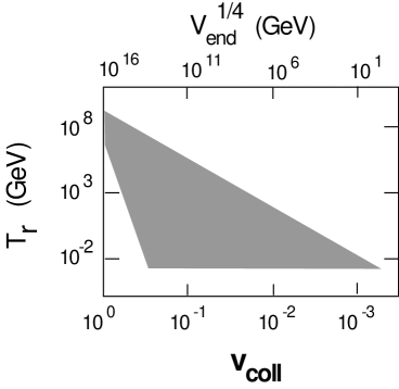
Figure 3: The region of parameter space within which the cyclic model is viable, assuming a potential of the general form shown in Figure 2. As well as the depth of the potential at kinetic domination, $V_{end}$, which determines the relative speed of the branes at collision, $V_{coll}$, the consistency of the model imposes constraints on the reheat temperature at the big bang, $T_{r}$.

Figure 5: The choice of timeslices is crucial in matching across the big crunch/big bang singularity. The brane collision (the $t=0$ surface, shown as a bold line) defines the natural matching surface. It is tempting to use $\delta\varphi=0$ slices defined from the four-dimensional effective theory. However, the $t=0^{-}$ and $t=0^{+}$ limits of these slices do not coincide with the brane collision surface, or with each other. The incoming $t=0^{-}$ surface lacks long wavelength curvature perturbations: however, curvature is induced when one changes to the brane-simultaneous collision surfaces. This curvature is transmitted to the comoving (or constant-energy density) slices of the outgoing big bang.

Figure 6: The global causal structure of the cyclic universe spacetime. The brane collision events define an infinite number of flat spacelike surfaces which tend, as $t\rightarrow-\infty$, to the null surface bisecting the diagram. As in inflation, a horizon is present, preventing an observer from seeing the entire universe. However, the sensitivity to initial conditions is arguably weaker in the cyclic model than in inflation because a very large (classically, infinite) number of cycles separates us from the null initial surface.

References

- [1] P. J. Steinhardt and N. Turok, Science 296, 1436 (2002); P. J. Steinhardt and N. Turok, Phys. Rev. D 65, 126003 (2002).
- [2] A. H. Guth, Phys. Rev. D 23, 347 (1981); A. D. Linde, Phys. Lett. B 108, 389 (1982); A. Albrecht and P. J. Steinhardt, Phys. Rev. Lett. 48, 1220 (1982).
- [3] J. Bardeen, P.J. Steinhardt, and M.S. Turner, Phys. Rev. D 28, 679 (1983); A.H. Guth and S.-Y. Pi, Phys. Rev. Lett. 49, 1110 (1982); S.W. Hawking, Phys. Lett. B 115, 295 (1982); A.A. Starobinskii, Phys. Lett.. B 117, 175 (1982).
- [4] J. Khoury, B. A. Ovrut, P. J. Steinhardt and N. Turok, Phys. Rev. D 64, 123522 (2001)
- [5] J. Khoury, B. A. Ovrut, N. Seiberg, P. J. Steinhardt and N. Turok, Phys. Rev. D 65, 086007 (2002). For recent work see M. Berkooz and B. Pioline, hep-th/0307280.
- [6] A. J. Tolley and N. Turok, Phys. Rev. D 66, 106005 (2002).
- [7] A. J. Tolley, N. Turok and P. J. Steinhardt, hep-th/0306109, Physical Review D, in press (2004).
- [8] J. Khoury, P. J. Steinhardt and N. Turok, Phys. Rev. Lett. in press (2004).
- [9] J. Khoury, P. J. Steinhardt and N. Turok, Phys. Rev. Lett. 91, 161301 (2003)
- [10] S. Gratton, J. Khoury, P. J. Steinhardt and N. Turok, astro-ph/0301395.
- [11] L. A. Boyle, P. J. Steinhardt and N. Turok, to appear (2004).
- [12] J. Khoury, B. A. Ovrut, P. J. Steinhardt and N. Turok, Phys. Rev. D 66, 046005 (2002).
- [13] D. Spergel et al., Astrophys. J. Suppl. 148 (2003) 175.
- [14] T. Damour, M. Henneaux, H. Nicolai, Class.Quant.Grav. 20 (2003) R145, hep-th/0212256.
- [15] G. Horowitz and J. Maldacena, hep-th/0310281.
- [16] G. Gottesman and J. Preskill, hep-th/0311269. Gottesman and Preskill criticise the proposal by pointing out how sensitive it is to interactions: for consistency the Hilbert space of states must be extremely carefully divided into two parts.
- [17] G. T. Horowitz and J. Polchinski, Phys. Rev. D 66, 103512 (2002).
- [18] H. Liu, G. Moore and N. Seiberg, JHEP 0206, 045 (2002); M. Fabinger and J. McGreevy, hep-th/0206196; M. Fabinger and S. Hellerman, hep-th/0212223.
- [19] D. Lyth, Phys. Lett. B 524, 1 (2002).
- [20] P. J. Steinhardt, A. J. Tolley and N. Turok, in preparation.
- [21] J. K. Erickson, D. H. Wesley, P. J. Steinhardt and N. Turok, hep-th/0312009.
- [22] The time delay is sometimes incorrectly referred to as a gauge mode, but it is not. As long as , the time delay mode cannot be gauged away.
- [23] R. Brustein, M. Gasperini, G. Veneziano, hep-th/9803018, Phys.Lett. B431 (1998) 277.
- [24] B. Craps and B.A. Ovrut, hep-th/0308057.
- [25] T. J. Battefield, S. P. Patil, and R. Brandenberger, hep-th/0401010.
- [26] G. Veneziano, Phys. Lett. B 265, 287 (1991); M. Gasperini and G. Veneziano, Astropart. Phys. 1, 317 (1993).
- [27] T. Banks and W. Fischler, hep-th/0212113, hep-th/0310288.