OUTP-04-07P

hep-th/0403003

February 2004

$SO(10)$ heterotic M-theory vacua

Abstract

The $SO(10)$ embedding of the Standard Model spectrum is supported by evidence for neutrino masses. This thesis adapts the available formalism to study a class of heterotic M-theory vacua with $SO(10)$ grand unification group. Compactification to four dimensions with $\mathcal{N}=1$ supersymmetry is achieved on a torus fibered Calabi-Yau 3-fold $\mathbf{Z}=\mathbf{X}/\tau_{\mathbf{X}}$ with first homotopy group $\pi_{1}(\mathbf{Z})=\mathbb{Z}_{2}$. Here $\mathbf{X}$ is an elliptically fibered Calabi-Yau 3-fold which admits two global sections and $\tau_{\mathbf{X}}$ is a freely acting involution on $\mathbf{X}$. The vacua in this class have net number of three generations of chiral fermions in the observable sector and may contain M5-branes in the bulk space which wrap holomorphic curves in $\mathbf{Z}$. Vacua with nonvanishing and vanishing instanton charges in the observable sector are considered. The latter case corresponds to potentially viable matter Yukawa couplings. Since $\pi_{1}(\mathbf{Z})=\mathbb{Z}_{2}$, the grand unification group can be broken with $\mathbb{Z}_{2}$ Wilson lines.

Realistic free-fermionic models preserve the $SO(10)$ embedding of the Standard Model spectrum. These models have a stage in their construction which corresponds to $\mathbb{Z}_{2}\times\mathbb{Z}_{2}$ orbifold compactification of the weakly coupled 10-dimensional heterotic string. This correspondence identifies associated Calabi-Yau 3-folds which possess the structure of the above $\mathbf{Z}$ and $\mathbf{X}$. This, in turn, allows the above formalism to be used to study heterotic M-theory vacua associated with realistic free-fermionic models. It is argued how the top quark Yukawa coupling in these models can be reproduced in the heterotic M-theory limit.

Chapter 1 Introduction

When the 11-dimensional supergravity [1] limit of M-theory [2] is compactified on an orbifold $\mathbf{S}^{1}/\mathbb{Z}_{2}$, cancellation of gauge and gravitational anomalies requires the presence of a chiral $\mathcal{N}=1$, $E_{8}$ vector supermultiplet on each of the two orbifold fixed planes. If the gauginos in these supermultiplets have opposite chirality, then one obtains a theory which has no spacetime supersymmetry [3]. On the other hand, if the gauginos have the same chirality, then one obtains a theory with $\mathcal{N}=1$ supersymmetry. This supersymmetric theory is known as Hořava-Witten theory [4, 5]; it gives the low-energy strongly coupled limit of the $E_{8}\times E_{8}$ heterotic string.

Compactifications of Hořava-Witten theory leading to unbroken $\mathcal{N}=1$ supersymmetry in four dimensions [6] are (to lowest order) based on the spacetime structure

$$\mathbf{M}^{11}=\mathbf{M}^{4}\times\mathbf{S}^{1}/\mathbb{Z}_{2}\times\boldsymbol{\mathcal{X}},$$ (1.1)

where $\mathbf{M}^{4}$ is 4-dimensional Minkowski space and $\boldsymbol{\mathcal{X}}$ is a Calabi-Yau 3-fold. Generally, on a given fixed plane, some subgroup $G$ of the $E_{8}$ symmetry survives on the Calabi-Yau 3-fold. $E_{8}$ is broken to $H$, where the grand unification group $H$ is the commutant subgroup of $G$ in $E_{8}$. Table 1.1 lists the commutant subroup of $G=SU(n)$ in $E_{8}$ for the cases $n=3,4,5$.

$$\begin{array}[]{c|c}G&H\\ \hline\cr SU(3)&E_{6}\\ SU(4)&SO(10)\\ SU(5)&SU(5)\end{array}$$

Table 1.1: Commutant subgroup $H$ of $G=SU(n)$ in $E_{8}$ for the cases $n=3,4,5$.

The ‘standard embedding’, in which the spin connection of the Calabi-Yau 3-fold is embedded in a $G=SU(3)$ subgroup of one of the $E_{8}$ gauge groups, corresponds to $H=E_{6}$. Vacua with nonstandard embeddings may contain M5-branes [6, 7] in the bulk space. One refers to Hořava-Witten theory compactified to lower dimensions with arbitrary gauge vacua as heterotic M-theory.

Powerful techniques in algebraic geometry have been developed which allow the study of a large class of the $G=SU(n)$ vacua discussed above. Consider a Calabi-Yau 3-fold $\boldsymbol{\mathcal{X}}$. The gauge fields associated with $G$ ‘live’ on $\boldsymbol{\mathcal{X}}$, and hence $(3+1)$-dimensional Poincaré invariance is left unbroken. The requirement of unbroken $\mathcal{N}=1$ supersymmetry implies that the corresponding field strengths must satisfy the Hermitian Yang-Mills constraints

$$F_{ab}=F_{\overline{a}\overline{b}}=g^{a\overline{b}}F_{a\overline{b}}=0.$$ (1.2)

Donaldson [8] and Uhlenbeck and Yau [9] prove that each solution to the 6-dimensional Yang-Mills equations

$$D^{A}F_{AB}=0$$ (1.3)

satisfying the Hermitian Yang-Mills constraints corresponds to a semistable holomorphic vector bundle $V_{\boldsymbol{\mathcal{X}}}$ over $\boldsymbol{\mathcal{X}}$ with structure group being the complexification $G_{\mathbb{C}}$ of the group $G$, and conversely. Whereas solving the above Yang-Mills equations may be untenable in practice, some methods for constructing semistable holomorphic vector bundles are known.

Semistable holomorphic vector bundles $V_{\mathbf{X}}$ with structure groups

$$G_{\mathbb{C}}=SU(n)_{\mathbb{C}}\subset E_{8\mathbb{C}}$$ (1.4)

can be explicitly constructed over an elliptically fibered Calabi-Yau 3-fold $\mathbf{X}$ using the spectral cover method [10, 11, 12]. That is, $\mathbf{X}$ is a torus fibered Calabi-Yau 3-fold which admits a global section. It consists of a complex base 2-surface $\mathbf{B}$ and elliptic curves $\mathbf{E}_{b}$ fibered over each point $b\in\mathbf{B}$. The Calabi-Yau condition

$$c_{1}(\mathbf{TX})=0$$ (1.5)

restricts the base $\mathbf{B}$ [13, 14] to be a del Pezzo $(\mathbf{dP}_{r},r=0,\dots,8)$, rational elliptic $(\mathbf{dP}_{9})$, Hirzebruch $(\mathbb{F}_{r},r\geq 0)$, blown-up Hirzebruch, or an Enriques surface. Donagi, Lukas, Ovrut and Waldram [15, 16] used the above construction and the results of [17, 18] to present a class of heterotic M-theory vacua. The vacua in this class have net number of generations $N_{\textrm{gen}}=3$ of chiral fermions in the observable sector with grand unification groups such as $H=E_{6}$, $SO(10)$, and $SU(5)$. The global section restricts the fundamental group of $\mathbf{X}$ to be trivial and hence Wilson lines cannot be used to break $H$ to the standard model gauge group. The exception is $\mathbf{X}$ fibered over an Enriques base which, however [16], is not consistent with the requirement $N_{\textrm{gen}}=3$. The vacua with nonstandard embeddings generically contain M5-branes in the bulk space at specific points in the $\mathbf{S}^{1}/\mathbb{Z}_{2}$ orbifold direction. These M5-branes are required to span the 4-dimensional uncompactified space (to preserve $(3+1)$-dimensional Poincaré invariance) and wrap holomorphic curves in $\mathbf{X}$ (to preserve $\mathcal{N}=1$ supersymmetry in four dimensions).

Considering instead torus fibered Calabi-Yau 3-folds which do not admit a global section, one expects to find nontrivial first homotopy groups. Such a 3-fold $\mathbf{Z}$ can be constructed from an elliptically fibered Calabi-Yau 3-fold $\mathbf{X}$ by modding out by a discrete group of freely acting symmetries $\Gamma$. The smooth 3-fold $\mathbf{Z}=\mathbf{X}/\Gamma$ has first homotopy group $\pi_{1}(\mathbf{Z})=\Gamma$. To construct semistable holomorphic vector bundles on $\mathbf{Z}$, one finds those bundles on $\mathbf{X}$ which are invariant under $\Gamma$. These then descend to bundles on $\mathbf{Z}$. Donagi, Ovrut, Pantev and Waldram [19, 20] used these results to construct $N_{\textrm{gen}}=3$ vacua with grand unification group $H=SU(5)$ which is broken to the standard model gauge group with a $\mathbb{Z}_{2}$ Wilson line. This was done by taking $\Gamma=\mathbb{Z}_{2}$ and constructing an elliptically fibered Calabi-Yau 3-fold $\mathbf{X}$ which admits two global sections and a freely acting involution

$$\tau_{\mathbf{X}}:\mathbf{X}\rightarrow\mathbf{X}.$$ (1.6)

The torus fibered Calabi-Yau 3-fold

$$\mathbf{Z}=\frac{\mathbf{X}}{\tau_{\mathbf{X}}}$$ (1.7)

has first homotopy group

$$\pi_{1}(\mathbf{Z})=\mathbb{Z}_{2}.$$ (1.8)

This thesis extends the above work by Donagi, Ovrut, Pantev and Waldram by considering the $H=SO(10)$ case. Hence the title ‘$SO(10)$ heterotic M-theory vacua’. The $SO(10)$ embedding of the Standard Model spectrum is supported by experimental evidence [21] for neutrino masses. A class of string models which preserves this embedding are the realistic free-fermionic models [22, 23, 24, 25]. These $N_{\textrm{gen}}=3$, 4-dimensional string models are constructed using the free-fermionic formulation [26] of the weakly coupled heterotic string. They have a stage in their construction which corresponds [27] to $\mathbb{Z}_{2}\times\mathbb{Z}_{2}$ orbifold compactification of the weakly coupled 10-dimensional heterotic string. This correspondence identifies associated Calabi-Yau 3-folds which possess the structure of the above $\mathbf{Z}$ and $\mathbf{X}$. This, in turn, allows the above formalism to be used to study heterotic M-theory vacua associated with the realistic free-fermionic models.

A free-fermionic model is generated by a suitable choice of boundary condition basis vectors (which encode the spin structure of the worldsheet fermions) and generalized GSO projection coefficients. The boundary condition basis vectors associated with the realistic free-fermionic models are constructed in two stages. The first stage constructs the NAHE set [28] of five basis vectors denoted by $\{\mathbf{1},\mathbf{S},\mathbf{b}_{1},\mathbf{b}_{2},\mathbf{b}_{3}\}$. After generalized GSO projections over the NAHE set, the residual gauge group is

$$SO(10)\times SO(6)^{3}\times E_{8}.$$

NAHE set models have $\mathcal{N}=1$ spacetime supersymmetry and 48 chiral generations in the $\mathbf{16}$ representation of $SO(10)$ (16 from each of the sectors $\mathbf{b}_{1}$, $\mathbf{b}_{2}$, and $\mathbf{b}_{3}$). The sectors $\mathbf{b}_{1}$, $\mathbf{b}_{2}$, and $\mathbf{b}_{3}$ correspond to the three twisted sectors of the associated $\mathbb{Z}_{2}\times\mathbb{Z}_{2}$ orbifold. The second stage of the construction adds three (or four) basis vectors, typically denoted by $\{\boldsymbol{\alpha},\boldsymbol{\beta},\boldsymbol{\gamma},\ldots\}$, which correspond to Wilson lines in the associated $\mathbb{Z}_{2}\times\mathbb{Z}_{2}$ orbifold formulation. These basis vectors break the $SO(10)\times SO(6)^{3}\times E_{8}$ gauge group and reduce the number of chiral generations from 48 to 3 (one from each of the sectors $\mathbf{b}_{1}$, $\mathbf{b}_{2}$, and $\mathbf{b}_{3}$). The $SO(10)$ symmetry is broken to one of its subgroups. The flipped $SU(5)$ [22], Pati-Salam [23], Standard-like [24], and left-right symmetric [25] $SO(10)$ breaking patterns are shown in Table 1.2.

$$\begin{array}[]{cl}\textrm{flipped}\ SU(5)&SO(10)\rightarrow SU(5)\times U(1)\\ \textrm{Pati-Salam}&SO(10)\rightarrow SO(6)\times SO(4)\\ \textrm{Standard-like}&SO(10)\rightarrow SU(3)\times SU(2)\times U(1)^{2}\\ \textrm{left-right symmetric}&SO(10)\rightarrow SU(3)\times SU(2)_{L}\times SU(2)_{R}\times U(1)\end{array}$$

Table 1.2: $SO(10)$ breaking patterns in realistic free-fermionic models.

In the former two cases, an additional $\mathbf{16}$ and $\mathbf{\overline{16}}$ representation of $SO(10)$ is obtained from the set $\{\boldsymbol{\alpha},\boldsymbol{\beta},\boldsymbol{\gamma},\ldots\}$. Similarly, the hidden $E_{8}$ is broken to one of its subgroups. The flavor $SO(6)$ symmetries are broken to flavor $U(1)$ symmetries. Three such symmetries arise from the subgroup of the observable $E_{8}$ which is orthogonal to $SO(10)$. Additional $U(1)$ symmetries arise from the pairing of real fermions. The final observable gauge group depends on the number of such pairings.

The precise geometrical realization of the full $N_{\textrm{gen}}=3$ realistic free-fermionic models is not yet known. However, the extended NAHE set $\{\mathbf{1},\mathbf{S},\\ \mathbf{b}_{1},\mathbf{b}_{2},\mathbf{b}_{3},\boldsymbol{\xi}_{1}\}$, or equivalently $\{\mathbf{1},\mathbf{S},\boldsymbol{\xi}_{1},\boldsymbol{\xi}_{2},\mathbf{b}_{1},\mathbf{b}_{2}\}$, has been shown [27] to yield the same data as the $\mathbb{Z}_{2}\times\mathbb{Z}_{2}$ orbifold of a toroidal Narain model [29] with nontrivial background fields [30]. This $\mathbb{Z}_{2}\times\mathbb{Z}_{2}$ orbifold is denoted by $\mathbf{Z}_{+}$ or $\mathbf{Z}_{-}$, depending on the choice of sign for the GSO projection coefficient $C(^{\boldsymbol{\xi_{1}}}_{\boldsymbol{\xi_{2}}})$. Each of the three twisted sectors produces eight chiral generations in the $\mathbf{27}$ representation of $E_{6}$ in the case of $\mathbf{Z}_{+}$, or $\mathbf{16}$ representation of $SO(10)$ in the case of $\mathbf{Z}_{-}$. The untwisted sector produces an additional three $\mathbf{27}$ and $\mathbf{\overline{27}}$ or $\mathbf{16}$ and $\mathbf{\overline{16}}$ repesentations of $E_{6}$ or $SO(10)$, respectively, yielding $N_{\textrm{gen}}=24$. As the NAHE set is common to all realistic free-fermionic models, $\mathbf{Z}_{+}$ and $\mathbf{Z}_{-}$ are at their core. A freely acting shift $\gamma$ relates the $(h^{(1,1)},h^{(2,1)})=(27,3)$ orbifold $\mathbf{Z}_{+}$ ($\mathbf{Z}_{-}$) to the $(h^{(1,1)},h^{(2,1)})=(51,3)$ orbifold $\mathbf{X}_{+}$ ($\mathbf{X}_{-}$). As will be discussed, the Calabi-Yau 3-folds associated with the (27,3) and (51,3) orbifolds have the structure of the above $\mathbf{Z}$ and $\mathbf{X}$.

The new results presented in this thesis have been published by Faraggi, Garavuso and Isidro [31] and Faraggi and Garavuso [32]. In the former work, it is shown that a class of $N_{\textrm{gen}}=3$, $H=SO(10)$ vacua is admitted by the $\mathbf{B}=\mathbb{F}_{2}$ surface, while the $\mathbf{B}=\mathbf{dP}_{3}$ surface does not admit such a class. Furthermore, $\mathbf{B}=\mathbb{F}_{r}$ $(r\ \textrm{even}\geq 4)$ admits this class when certain conditions are satisfied, while $\mathbf{B}=\mathbb{F}_{0}$ and $\mathbf{B}=\mathbb{F}_{r}$ $(r\ \textrm{odd}\geq 1)$ do not admit this class. The $SO(10)$ symmetry is broken to $SU(5)\times U(1)$ with a $\mathbb{Z}_{2}$ Wilson line. Such vacua are concrete realizations of the heterotic M-theory brane-world shown in Figure 1.1.

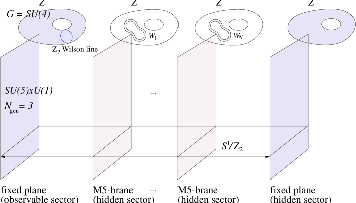
Figure 1.1: Heterotic M-theory brane-world. A $\mathbb{Z}_{2}$ Wilson line breaks the $SO(10)$ grand unification group to $SU(5)\times U(1)$ with $N_{\textrm{gen}}=3$ net chiral generations in the observable sector. There are $N$ M5-branes wrapping holomorphic curves $W^{(n)}_{\mathbf{Z}}$ $(n=1,\ldots,N)$ in the torus fibered Calabi-Yau 3-fold $\mathbf{Z}$.

Finally, the former work utilizes the $\mathbb{Z}_{2}\times\mathbb{Z}_{2}$ correspondence to connect realistic free-fermionic models to the above formalism. In the latter work, vacua with potentially viable matter Yukawa couplings are searched for. Arnowitt and Dutta [33] argue that such vacua can be obtained by requiring vanishing instanton charges in the observable sector. This restriction rules out the solutions found in [31]. However, by replacing the previously considered sufficient (but not necessary) constraints on the vector bundles with more general constraints, it is shown that a class of $N_{\textrm{gen}}=3$, $H=SO(10)$ vacua with potentially viable matter Yukawa couplings is admitted by $\mathbf{B}=\mathbf{dP}_{7}$ when certain conditions are satisfied, while $\mathbf{B}=\mathbf{dP}_{r}$ $(r=0,\ldots,6,8)$ and $\mathbf{B}=\mathbb{F}_{r}$ $(r\geq 0)$ do not admit such a class. It is then argued how the top quark Yukawa coupling [34] in realistic free-fermionic models can be reproduced in the heterotic M-theory limit. Although the precise geometrical realization of the full $N_{\textrm{gen}}=3$ models is unknown, this coupling can be computed as a $\mathbf{27}^{3}$ $E_{6}$ or $\mathbf{16}\cdot\mathbf{16}\cdot\mathbf{10}$ $SO(10)$ coupling with $N_{\textrm{gen}}=24$. This leads to the presentation of rules for constructing heterotic M-theory vacua allowing $H=E_{6}$ and $SO(10)$ grand unification groups with arbitrary $N_{\textrm{gen}}$.

The presentation is organized as follows: Chapter 2 reviews Hořava-Witten theory, its compactification to four dimensions with $\mathcal{N}=1$ supersymmetry, and the associated 4-dimensional low energy effective action. Chapter 3 discusses rules for constructing heterotic M-theory vacua allowing grand unification groups such as $H=E_{6}$, $SO(10)$, and $SU(5)$ with arbitrary $N_{\textrm{gen}}$. The vacua appearing in [31] and [32] are presented in Chapters 4 and 5, respectively. Chapter 6 reviews realistic free-fermionic models and their $\mathbb{Z}_{2}\times\mathbb{Z}_{2}$ correspondence in more detail, explains how this correspondence identifies associated Calabi-Yau 3-folds which possess the structure of the above $\mathbf{Z}$ and $\mathbf{X}$, and argues how the top quark Yukawa coupling in realistic free-fermionic models can be reproduced in the heterotic M-theory limit. Chapter 7 summarizes the new results presented in this thesis. Appendix A reviews Chern classes. The spectral cover method is reviewed in Appendix B.

Chapter 2 Heterotic M-theory

M-theory on the orbifold $\mathbf{S}^{1}/\mathbb{Z}_{2}$ is believed to describe the strong coupling limit of the $E_{8}\times E_{8}$ heterotic string [4]. At low energy, this theory is described by 11-dimensional supergravity [1] coupled to one 10-dimensional $E_{8}$ Yang-Mills supermultiplet on each of the two orbifold fixed planes. This low energy description, known as Hořava-Witten theory [5], will be summarized in Section 2.1. As discussed in Chapter 1, Hořava-Witten theory compactified to lower dimensions with arbitrary gauge vacua is referred to as heterotic M-theory. Compactification on a Calabi-Yau 3-fold to four dimensions with unbroken $\mathcal{N}=1$ supersymmetry [6] is reviewed in Section 2.2, and the corresponding 4-dimensional effective theory is discussed in Section 2.3.

The following conventions will be employed. The 11-dimensional space $\mathbf{M}^{11}$ is parameterized by coordinates $x^{I}$ with indices

$$I,J,K,\ldots=0,\ldots,9,11.$$ (2.1)

The metric

$$g_{IJ}=\eta_{mn}e^{m}_{I}e^{n}_{J}$$ (2.2)

has Lorentz signature $(-,+,\ldots,+)$. The $32\times 32$ real gamma matrices satisfy

$$\{\Gamma_{I},\Gamma_{J}\} =2g_{IJ}$$ (2.3)

$$\Gamma_{0}\ldots\Gamma_{9}\Gamma_{11} =1,$$ (2.4)

and

$$\Gamma^{I_{1}\ldots I_{n}}\equiv\Gamma^{[I_{1}}\ldots\Gamma^{I_{n}]}.$$ (2.5)

The orbifold $\mathbf{S}^{1}/\mathbb{Z}_{2}$ is chosen to be tangent to $x^{11}$, with $\mathbb{Z}_{2}$ acting as

$$\mathbb{Z}_{2}:x^{11}\rightarrow-x^{11}.$$ (2.6)

Barred indices

$$\bar{I},\bar{J},\bar{K},\ldots=0,\ldots,9$$ (2.7)

are used to label the coordinates of the 10-dimensional space orthogonal to the orbifold. In the upstairs picture, $x^{11}\in[-\pi\rho,\pi\rho]$ with the endpoints identified. There are two 10-dimensional hyperplanes, $\mathbf{M}^{10}_{\textrm{\tiny{($i$)}}}\ (i=1,2)$, locally specified by $x^{11}=0$ and $x^{11}=\pi\rho$, which are fixed under $\mathbb{Z}_{2}$ action. In other words, the orbifold is a circle $\mathbf{S}^{1}$ of radius $\rho$ with fixed points at $x^{11}=0$ and $x^{11}=\pi\rho$. In the downstairs picture, the orbifold is an interval $x^{11}\in[0,\pi\rho]$ with $\mathbf{M}^{10}_{\textrm{\tiny{($i$)}}}$ $(i=1,2)$ forming boundaries to $\mathbf{M}^{11}$. The fields are required to have a definite behavior under the $\mathbb{Z}_{2}$ action. A bosonic field $\Phi$ must be even or odd; that is,

$$\Phi(x^{11})=\pm\Phi(-x^{11}).$$ (2.8)

For an 11-dimensional Majorana spinor $\Psi$, the condition is

$$\Psi(x^{11})=\pm\Gamma_{11}\Phi(-x^{11})$$ (2.9)

so that the projection to an orbifold fixed plane yields a 10-dimensional Majorana-Weyl spinor. The 11-dimensional supergravity multiplet consists of the metric $g_{IJ}$, a 3-form potential $C_{IJK}$ with field strength $G_{IJKL}=d_{I}C_{JKL}=4!\,\partial_{[I}C_{JKL]}$, and the gravitino $\psi_{I\alpha}$ ($\alpha$ is a 32-component Majorana spinor index). For the bosonic fields, $g_{\bar{I}\bar{J}}$, $g_{11,11}$ and $C_{\bar{I}\bar{J}11}$ must be even under $\mathbb{Z}_{2}$, while $g_{\bar{I}11}$ and $C_{\bar{I}\bar{J}\bar{K}}$ must be odd. For the 11-dimensional gravitino, the condition is

$$\psi_{\bar{I}}(x^{11})=\Gamma_{11}\psi_{\bar{I}}(-x^{11}),\quad\psi_{11}(x^{11})=-\Gamma_{11}\psi_{11}(-x^{11}).$$ (2.10)

The 11-dimensional supergravity multiplet is coupled to one $E_{8}$ Yang-Mills supermultiplet $(A^{\textrm{\tiny{($i$)}}a}_{\bar{I}},\chi^{\textrm{\tiny{($i$)}}a})$ on each orbifold fixed plane $\mathbf{M}^{10}_{\textrm{\tiny{($i$)}}}$ $(i=1,2)$. Here, $a=1,\ldots,248$ labels the adjoint representation of $E_{8}$. The $E_{8}$ gauge field $A^{\textrm{\tiny{($i$)}}}_{\bar{I}}$ has field strength

$$F^{\textrm{\tiny{($i$)}}}_{\bar{I}\bar{J}}=\partial_{\bar{I}}A^{\textrm{\tiny{($i$)}}}_{\bar{J}}-\partial_{\bar{J}}A^{\textrm{\tiny{($i$)}}}_{\bar{I}}+[A^{\textrm{\tiny{($i$)}}}_{\bar{I}},A^{\textrm{\tiny{($i$)}}}_{\bar{J}}],$$ (2.11)

and the gaugino $\chi^{\textrm{\tiny{($i$)}}}$ satisfies

$$\Gamma_{11}\chi^{\textrm{\tiny{($i$)}}}=\chi^{\textrm{\tiny{($i$)}}}.$$ (2.12)

An inner product is defined by

$$X^{a}X^{a}=\textrm{tr}(X^{2})=\frac{1}{30}\textrm{Tr}(X^{2}),$$ (2.13)

with ‘Tr’ the trace in the adjoint representation. The spin connection

$$\Omega_{IJK}\equiv\Omega^{mn}_{I}e_{Jm}e_{Kn}$$ (2.14)

is understood to be given by the solution of the field equation that results from varying it as an independent field. The Riemann tensor is the field strength constructed from $\Omega$. When the theory is further compactified on a Calabi-Yau manifold in Section 2.2, indices

$$A,B,C,\ldots=4,\ldots,9$$ (2.15)

label the Calabi-Yau coordinates. Holomorphic and antiholomorphic indices on the Calabi-Yau space are denoted by $a,b,c,\ldots$ and $\bar{a},\bar{b},\bar{c},\ldots$, respectively. Coordinates of the 4-dimensional uncompactified space $\mathbf{M}^{4}$ are labeled by indices

$$\mu,\nu,\ldots=0,\ldots,3.$$ (2.16)

2.1 Hořava-Witten theory

Hořava-Witten theory can be formulated as an expansion [5] in the 11-dimensional gravitational coupling $\kappa$. To lowest order in this expansion, Hořava-Witten theory is 11-dimensional supergravity (which is of order $\kappa^{-2}$), with the fields restricted under the $\mathbb{Z}_{2}$ action as described above. In the upstairs picture, the action is

$$S_{\textrm{SG}}=-\frac{1}{\kappa^{2}}\int_{\mathbf{M}^{11}}d^{11}x\sqrt{g}\Biggl{[}\frac{1}{2}R+\frac{1}{2}\overline{\psi}_{I}\Gamma^{IJK}D_{J}(\Omega)\psi_{K}+\frac{1}{48}G_{IJKL}G^{IJKL}\Biggr{.}\\ +\frac{\sqrt{2}}{192}\left(\overline{\psi}_{I}\Gamma^{IJKLMN}\psi_{N}+12\overline{\psi}^{J}\Gamma^{KL}\psi^{M}\right)G_{JKLM}\\ \left.+\frac{\sqrt{2}}{3456}\epsilon^{I_{1}\ldots I_{11}}C_{I_{1}I_{2}I_{3}}G_{I_{4}\ldots I_{7}}G_{I_{8}\ldots I_{11}}+\textrm{(Fermi)}^{4}\right].$$ (2.17)

The terms which are quartic in the gravitino can be absorbed into the definition of supercovariant objects. The condition (2.10) means that the gravitino is chiral from a 10-dimensional perspective, and so the theory has a gravitational anomaly localized on the fixed planes. $S_{\textrm{SG}}$ is invariant under the local supersymmetry transformations

$$\delta e_{I}^{m} =\frac{1}{2}\bar{\eta}\Gamma^{m}\psi_{I}$$ (2.18)

$$\delta C_{IJK} =-\frac{\sqrt{2}}{8}\bar{\eta}\Gamma_{[IJ}\psi_{K]}$$ (2.19)

$$\delta\psi_{I} =D_{I}(\Omega)\eta+\frac{\sqrt{2}}{288}(\Gamma_{IJKLM}-8g_{IJ}\Gamma_{KLM})G^{JKLM}\eta+(\textrm{Fermi})^{2}$$ (2.20)

whose infinitesimal spacetime dependent Grassmann parameter $\eta$ (which transforms as a Majorana spinor) satisfies the orbifold condition

$$\eta(x^{11})=\Gamma_{11}\eta(-x^{11}).$$ (2.21)

This condition means that the theory has 32 supersymmetries in the bulk, but only 16 (chiral) supersymmetries on the orbifold fixed planes. At this order in $\kappa$, the 4-form field strength $G_{IJKL}$ satisfies the boundary conditions

$$G_{\bar{I}\bar{J}\bar{K}\bar{L}}|_{x^{11}=0} =0$$ (2.22)

$$G_{\bar{I}\bar{J}\bar{K}\bar{L}}|_{x^{11}=\pi\rho} =0,$$ (2.23)

the equation of motion

$$D_{I}(\Omega)G^{IJKL}=0,$$ (2.24)

and the Bianchi identity

$$(dG)_{IJKLM}=0.$$ (2.25)

To this order, it is consistent to set $G_{IJKL}=0$.

Cancellation of the gravitational anomaly requires the introduction of one $E_{8}$ Yang-Mills supermultiplet $(A^{\textrm{\tiny{($i$)}}a}_{\bar{I}},\chi^{\textrm{\tiny{($i$)}}a})$ on each orbifold fixed plane $\mathbf{M}^{10}_{\textrm{\tiny{($i$)}}}$ $(i=1,2)$. The minimal Yang-Mills action is

$$S_{\textrm{YM}}=-\frac{1}{\lambda^{2}}\sum_{i=1}^{2}\int_{\mathbf{M}^{10}_{\textrm{\tiny{($i$)}}}}d^{10}x\sqrt{g}\ \textrm{tr}\left(\frac{1}{4}F^{\textrm{\tiny{($i$)}}}_{\bar{I}\bar{J}}F^{\textrm{\tiny{($i$)}}\bar{I}\bar{J}}+\frac{1}{2}\bar{\chi}^{\textrm{\tiny{($i$)}}}\Gamma^{\bar{I}}D_{\bar{J}}(\Omega)\chi^{\textrm{\tiny{($i$)}}}\right)$$ (2.26)

where $\lambda$ is the 10-dimensional gauge coupling. This action is invariant under the global supersymmetry transformations

$$\delta A^{\textrm{\tiny{($i$)}}a}_{\bar{I}} =\frac{1}{2}\bar{\eta}\Gamma_{\bar{I}}\chi^{\textrm{\tiny{($i$)}}a}$$ (2.27)

$$\delta\chi^{\textrm{\tiny{($i$)}}a} =-\frac{1}{4}\Gamma^{\bar{I}\bar{J}}F^{\textrm{\tiny{($i$)}}a}_{\bar{I}\bar{J}}\eta.$$ (2.28)

The challenge is then to add interactions and modify the supersymmetry transformation laws so that $S=S_{\textrm{SG}}+S_{\textrm{YM}}+\cdots$ is locally supersymmetric. This involves coupling the gravitino to the Yang-Mills supercurrent. However, since the gravitino lives in the 11-dimensional bulk, while the Yang-Mills supermultiplets live on the 10-dimensional fixed planes, a locally supersymmetric theory cannot be achieved simply by adding interactions on the fixed planes. To achieve local supersymmetry, the Bianchi identity must be modified to read

$$(dG)_{11\bar{I}\bar{J}\bar{K}\bar{L}}=8\pi^{2}\sqrt{2}\ \frac{\kappa^{2}}{\lambda^{2}}\Biggl{\{}J^{(0)}\delta(x^{11})+J^{(N+1)}\delta(x^{11}-\pi\rho)\Biggr{.}\\ \Biggl{.}+\frac{1}{2}\sum_{n=1}^{N}J^{(n)}\left[\delta(x^{11}-x_{n})+\delta(x^{11}+x_{n})\right]\Biggr{\}}_{\bar{I}\bar{J}\bar{K}\bar{L}}$$ (2.29)

where

$$J^{(0)} =-\frac{1}{16\pi^{2}}\left[\textrm{tr}\left(F^{\textrm{\tiny{(1)}}}\wedge F^{\textrm{\tiny{(1)}}}\right)-\frac{1}{2}\,\textrm{tr}\,(R\wedge R)\right]_{x^{11}=0}$$ (2.30)

$$J^{(N+1)} =-\frac{1}{16\pi^{2}}\left[\textrm{tr}\left(F^{\textrm{\tiny{(2)}}}\wedge F^{\textrm{\tiny{(2)}}}\right)-\frac{1}{2}\,\textrm{tr}\,(R\wedge R)\right]_{x^{11}=\pi\rho}$$ (2.31)

are the sources on the fixed planes at $x^{11}=x_{0}\equiv 0$ and $x^{11}=x_{N+1}\equiv\pi\rho$, respectively, and $J^{(n)}$ $(n=1,\ldots,N)$ are the M5-brane sources located at $x^{11}=x_{1},\ldots,x_{N}$ $(0\leq x_{1}\leq\ldots\leq x_{N}\leq\pi\rho)$. Each M5-brane at $x=x_{n}$ is paired with a mirror M5-brane at $x=-x_{n}$ with the same source since the Bianchi identity must be even under the $\mathbb{Z}_{2}$ action.

With the modified Bianchi identity (2.29), $S=S_{\textrm{SG}}+S_{\textrm{YM}}+\ldots$ can be made locally supersymmetric. However, having gained supersymmetry, Yang Mills gauge invariance has been lost. The modified Bianchi identity implies that $G_{11\bar{I}\bar{J}\bar{K}}$ is invariant under the infinitesimal gauge transformations

$$\delta A^{\textrm{\tiny{($i$)}}a}_{\bar{I}}=D_{\bar{I}}(\Omega)\epsilon^{\textrm{\tiny{($i$)}}a}$$ (2.32)

if $C_{11\bar{I}\bar{J}}$ transforms as

$$\delta C_{11\bar{I}\bar{J}}=-\frac{\kappa^{2}}{6\sqrt{2}\lambda^{2}}\left[\delta(x^{11})\ \textrm{tr}\left(\epsilon^{\textrm{\tiny{(1)}}}F^{\textrm{\tiny{(1)}}}_{\bar{I}\bar{J}}\right)+\delta(x^{11}-\pi\rho)\ \textrm{tr}\left(\epsilon^{\textrm{\tiny{(2)}}}F^{\textrm{\tiny{(2)}}}_{\bar{I}\bar{J}}\right)\right].$$ (2.33)

This implies that the $CGG$ Chern-Simons interaction is not gauge invariant. Thus, the classical theory is not gauge invariant, and a consistent classical theory does not exist. At the quantum level, there is in addition the 10-dimensional Majorana-Weyl anomaly which cancels the gauge anomaly of the CGG interaction provided

$$\frac{1}{\lambda^{2}}=\frac{1}{2\pi\kappa^{2}}\left(\frac{\kappa}{4\pi}\right)^{2/3}.$$ (2.34)

The quantum theory is anomaly free; gauge, gravitational and mixed anomalies are cancelled with a refinement [4, 5] of the standard Green-Schwarz mechanism [35].

To order $\kappa^{-2+(2/3)}$, the Hořava-Witten action is

$$S=-\frac{1}{\kappa^{2}}\int_{\mathbf{M}^{11}}d^{11}x\sqrt{g}\Biggl{[}\frac{1}{2}R+\frac{1}{2}\overline{\psi}_{I}\Gamma^{IJK}D_{J}\left(\textrm{\scriptsize$\frac{1}{2}$}(\Omega+\hat{\Omega})\right)\psi_{K}\Biggr{.}\\ +\frac{\sqrt{2}}{384}\left(\overline{\psi}_{I}\Gamma^{IJKLMN}\psi_{N}+12\overline{\psi}^{J}\Gamma^{KL}\psi^{M}\right)(G_{JKLM}+\hat{G}_{JKLM})\\ \left.+\frac{1}{48}G_{IJKL}G^{IJKL}+\frac{\sqrt{2}}{3456}\epsilon^{I_{1}\ldots I_{11}}C_{I_{1}I_{2}I_{3}}G_{I_{4}\ldots I_{7}}G_{I_{8}\ldots I_{11}}\right]\\ -\frac{1}{2\pi\kappa^{2}}\left(\frac{\kappa}{4\pi}\right)^{2/3}\sum_{i=1}^{2}\int_{\mathbf{M}^{10}_{\textrm{\tiny{($i$)}}}}d^{10}x\sqrt{g}\Biggl{[}\frac{1}{4}F^{\textrm{\tiny{($i$)}}a}_{\bar{I}\bar{J}}F^{\textrm{\tiny{($i$)}}a\bar{I}\bar{J}}+\frac{1}{2}\bar{\chi}^{\textrm{\tiny{($i$)}}a}\Gamma^{\bar{I}}D_{\bar{J}}(\hat{\Omega})\chi^{\textrm{\tiny{($i$)}}a}\Biggr{.}\\ \left.+\frac{1}{8}\bar{\psi}_{I}\Gamma^{\bar{J}\bar{K}}\Gamma^{\bar{I}}\left(F^{\textrm{\tiny{($i$)}}a}_{\bar{J}\bar{K}}+\hat{F}^{\textrm{\tiny{($i$)}}a}_{\bar{J}\bar{K}}\right)\chi^{\textrm{\tiny{($i$)}}a}-\frac{\sqrt{2}}{48}\bar{\chi}^{\textrm{\tiny{($i$)}}a}\Gamma^{\bar{I}\bar{J}\bar{K}}\chi^{\textrm{\tiny{($i$)}}a}\hat{G}_{\bar{I}\bar{J}\bar{K}11}\right].$$ (2.35)

where the quartic Fermi terms are absorbed into the supercovariant objects

$$\hat{\Omega}_{IJK} =\Omega_{IJK}+\frac{1}{8}\bar{\psi}^{L}\Gamma_{LIJKM}\psi^{M}$$ (2.36)

$$\hat{G}_{IJKL} =G_{IJKL}+\frac{3\sqrt{2}}{4}\bar{\psi}_{[I}\Gamma_{JK}\psi_{L]}$$ (2.37)

$$\hat{F}^{\textrm{\tiny{($i$)}}a}_{\bar{I}\bar{J}} =F^{\textrm{\tiny{($i$)}}a}_{\bar{I}\bar{J}}-\bar{\psi}_{[\bar{I}}\Gamma_{\bar{J}\,]}\chi^{\textrm{\tiny{($i$)}}a}.$$ (2.38)

This action is invariant under the local supersymmetry transformations

$$\delta e_{I}^{m} =\frac{1}{2}\bar{\eta}\Gamma^{m}\psi_{I}$$ (2.39)

$$\delta C_{IJK}\ \textrm{is given by (\ref{superC}) with correction}\ \delta^{\prime}C_{11\bar{J}\bar{K}}$$ (2.40)

$$\delta\psi_{\bar{I}} =D_{\bar{I}}(\hat{\Omega})\eta+\frac{\sqrt{2}}{288}(\Gamma_{\bar{I}JKLM}-8g_{\bar{I}J}\Gamma_{KLM})\hat{G}^{JKLM}\eta+\delta^{\prime}\psi_{\bar{I}}$$ (2.41)

$$\delta\psi_{11} =D_{11}(\hat{\Omega})\eta+\frac{\sqrt{2}}{288}(\Gamma_{11JKLM}-8g_{11J}\Gamma_{KLM})\hat{G}^{JKLM}\eta+\delta^{\prime}\psi_{11}$$ (2.42)

$$\delta A^{\textrm{\tiny{($i$)}}a}_{\bar{I}} =\frac{1}{2}\bar{\eta}\Gamma_{\bar{I}}\chi^{\textrm{\tiny{($i$)}}a}$$ (2.43)

$$\delta\chi^{\textrm{\tiny{($i$)}}a} =-\frac{1}{4}\Gamma^{\bar{I}\bar{J}}F^{\textrm{\tiny{($i$)}}a}_{\bar{I}\bar{J}}\eta+\delta^{\prime}\chi^{\textrm{\tiny{($i$)}}a}$$ (2.44)

where the supersymmetry transformation law corrections are

$$\delta^{\prime}C_{11\bar{J}\bar{K}} =\frac{1}{6\sqrt{2}}\,\frac{1}{2\pi}\left(\frac{\kappa}{4\pi}\right)^{2/3}\sum_{i=1}^{2}\textrm{tr}\left(A^{\textrm{\tiny{($i$)}}}_{\bar{J}}\delta A^{\textrm{\tiny{($i$)}}}_{\bar{K}}-A^{\textrm{\tiny{($i$)}}}_{\bar{K}}\delta A^{\textrm{\tiny{($i$)}}}_{\bar{J}}\right)$$ (2.45)

$$\delta^{\prime}\psi_{\bar{I}} =-\frac{1}{576\pi}\left(\frac{\kappa}{4\pi}\right)^{2/3}\left[\delta(x^{11})\,\bar{\chi}^{\textrm{\tiny{(1)}}a}\Gamma^{\bar{J}\bar{K}\bar{L}}\chi^{\textrm{\tiny{(1)}}a}\right.$$

$$\left.\quad\quad\quad+\,\delta(x^{11}-\pi\rho)\,\bar{\chi}^{\textrm{\tiny{(2)}}a}\Gamma^{\bar{J}\bar{K}\bar{L}}\chi^{\textrm{\tiny{(2)}}a}\right]\left(\Gamma_{\bar{J}\bar{K}\bar{L}}-6g_{\bar{I}\bar{J}}\Gamma_{\bar{K}\bar{L}}\right)\eta$$ (2.46)

$$\delta^{\prime}\psi_{11} =+\frac{1}{576\pi}\left(\frac{\kappa}{4\pi}\right)^{2/3}\left[\delta(x^{11})\,\bar{\chi}^{\textrm{\tiny{(1)}}a}\Gamma^{JKL}\chi^{\textrm{\tiny{(1)}}a}\right.$$

$$\left.\quad\quad\quad\quad\quad\quad\quad+\,\delta(x^{11}-\pi\rho)\,\bar{\chi}^{\textrm{\tiny{(2)}}a}\Gamma^{JKL}\chi^{\textrm{\tiny{(2)}}a}\right]\Gamma_{JKL}\,\eta$$ (2.47)

$$\delta^{\prime}\chi^{\textrm{\tiny{($i$)}}a} =\frac{1}{4}\bar{\psi}_{\bar{I}}\Gamma_{\bar{J}}\chi^{\textrm{\tiny{($i$)}}a}\Gamma^{\bar{I}\bar{J}}\eta.$$ (2.48)

At this order in $\kappa$, the 4-form field strength $G_{IJKL}$ satisfies the boundary conditions

$$G_{\bar{I}\bar{J}\bar{K}\bar{L}}|_{x^{11}=0} =-\frac{3}{\sqrt{2}}\,\frac{1}{2\pi}\left(\frac{\kappa}{4\pi}\right)^{2/3}\left(F^{\textrm{\tiny{(1)}}a}_{[\bar{I}\bar{J}}F^{\textrm{\tiny{(1)}}a}_{\bar{K}\bar{L}]}-\frac{1}{2}\,\textrm{tr}\,R_{[\bar{I}\bar{J}}R_{\bar{K}\bar{L}]}\right)$$ (2.49)

$$G_{\bar{I}\bar{J}\bar{K}\bar{L}}|_{x^{11}=\pi\rho} =+\frac{3}{\sqrt{2}}\,\frac{1}{2\pi}\left(\frac{\kappa}{4\pi}\right)^{2/3}\left(F^{\textrm{\tiny{(2)}}a}_{[\bar{I}\bar{J}}F^{\textrm{\tiny{(2)}}a}_{\bar{K}\bar{L}]}-\frac{1}{2}\,\textrm{tr}\,R_{[\bar{I}\bar{J}}R_{\bar{K}\bar{L}]}\right),$$ (2.50)

the equation of motion

$$D_{I}(\Omega)G^{IJKL}=0,$$ (2.51)

and the Bianchi identity

$$(dG)_{11\bar{I}\bar{J}\bar{K}\bar{L}}=4\sqrt{2}\pi\left(\frac{\kappa}{4\pi}\right)^{2/3}\Biggl{\{}J^{(0)}\delta(x^{11})+J^{(N+1)}\delta(x^{11}-\pi\rho)\Biggr{.}\\ \Biggl{.}+\frac{1}{2}\sum_{n=1}^{N}J^{(n)}\left[\delta(x^{11}-x_{n})+\delta(x^{11}+x_{n})\right]\Biggr{\}}_{\bar{I}\bar{J}\bar{K}\bar{L}}.$$ (2.52)

Note that the $\textrm{tr}\,(R\wedge R)$ terms appearing in the above boundary conditions and Bianchi identity are not required by the low energy theory, but (since they are needed for anomaly cancellation, given the structure of the one-loop chiral anomalies) must be present in the full quantum M-theory.

2.2 Compactification to $D=4$ with $\mathcal{N}=1$

The compactification of Hořava-Witten theory to four dimensions with unbroken $\mathcal{N}=1$ supersymmetry is discussed in [6]. The procedure starts with the spacetime structure

$$\mathbf{M}^{11}=\mathbf{M}^{4}\times\mathbf{Z}\times\mathbf{S}^{1}/\mathbb{Z}_{2},$$ (2.53)

where $\mathbf{M}^{4}$ is 4-dimensional Minkowski space and $\mathbf{Z}$ is a Calabi-Yau 3-fold. M5-branes can be included in the bulk space at points throughout the orbifold interval. These M5-branes are required to span $\mathbf{M}^{4}$ (to preserve $(3+1)$-dimensional Poincaré invariance) and wrap holomorphic curves in $\mathbf{Z}$ (to preserve $\mathcal{N}=1$ supersymmetry in four dimensions).

The correction to the background (2.53) is computed perturbatively. The set of equations to be solved consists of the Killing spinor equation

$$\delta\psi_{I}=D_{I}\eta+\frac{\sqrt{2}}{288}(\Gamma_{IJKLM}-8g_{IJ}\Gamma_{KLM})G^{JKLM}\eta=0,$$ (2.54)

the equation of motion

$$D_{I}G^{IJKL}=0,$$ (2.55)

and the Bianchi identity

$$(dG)_{11\bar{I}\bar{J}\bar{K}\bar{L}}=4\sqrt{2}\pi\left(\frac{\kappa}{4\pi}\right)^{2/3}\Biggl{\{}J^{(0)}\delta(x^{11})+J^{(N+1)}\delta(x^{11}-\pi\rho)\Biggr{.}\\ \Biggl{.}+\frac{1}{2}\sum_{n=1}^{N}J^{(n)}\left[\delta(x^{11}-x_{n})+\delta(x^{11}+x_{n})\right]\Biggr{\}}_{\bar{I}\bar{J}\bar{K}\bar{L}}.$$ (2.56)

The Bianchi identity (2.56) can be viewed as an expansion in powers of $\kappa^{2/3}$. To linear order in $\kappa^{2/3}$, the solution to the Killing spinor equation, equation of motion, and Bianchi identity takes the form

$$(ds)^{2}=(1+b)\eta_{\mu\nu}dx^{\mu}dx^{\nu}+(g^{\textrm{\tiny{(CY)}}}_{AB}+h_{AB})dx^{A}dx^{B}+(1+\gamma)\left(dx^{11}\right)^{2}$$ (2.57)

$$\begin{aligned} G_{ABCD}&=0+G^{\prime}_{ABCD}\\ G_{ABC11}&=0+G^{\prime}_{ABC11}\\ \eta&=(1+\psi)\eta^{\textrm{\tiny{(CY)}}}.\end{aligned}$$ (2.58)

with all other components of $G_{IJKL}$ vanishing. $g^{\textrm{\tiny{(CY)}}}_{AB}$ and $\eta^{\textrm{\tiny{(CY)}}}$ are the Ricci-flat metric and the covariantly constant spinor on the Calabi-Yau 3-fold.

As discussed in [36], the first order corrections $b$, $h_{AB}$, $\gamma$, $G^{\prime}$ and $\psi$ can be expressed in terms of a single $(1,1)$-form $\mathcal{B}_{a\bar{b}}$ on the Calabi-Yau 3-fold. The results are

$$b =\frac{\sqrt{2}}{6}\beta$$ (2.59)

$$h_{a\bar{b}} =\sqrt{2}i\left(\beta_{a\bar{b}}-\frac{1}{3}\omega_{a\bar{b}}\beta\right)$$ (2.60)

$$\gamma =-\frac{\sqrt{2}}{3}\beta$$ (2.61)

$$G^{\prime}_{ABCD} =\frac{1}{2}\epsilon_{ABCDEF}\partial_{11}\beta^{EF}$$ (2.62)

$$G^{\prime}_{ABC11} =\frac{1}{2}\epsilon_{ABCDEF}\partial^{D}\beta^{EF}$$ (2.63)

$$\psi =-\frac{\sqrt{2}}{24}\beta$$ (2.64)

where $\beta=\omega^{AB}\beta_{AB}$ and $\omega_{a\bar{b}}=-ig^{\textrm{\tiny{(CY)}}}_{a\bar{b}}$ is the Kähler form. All that remains then is to determine $\mathcal{B}_{a\overline{b}}$, which can be expanded in terms of eigenmodes of the Laplacian on the Calabi-Yau 3-fold. For the purpose of computing low energy effective actions, it is sufficient to keep only the zero eigenvalue or ‘massless’ terms in this expansion; that is, the terms proportional to the harmonic $(1,1)$ forms of the Calabi-Yau 3-fold. Let $\{\omega_{ia\bar{b}}\}$ be a basis for these harmonic $(1,1)$-forms, where $i=1,\ldots,h^{(1,1)}$. Then

$$\mathcal{B}_{a\bar{b}}=\sum_{i}b_{i}\omega^{i}_{a\bar{b}}+(\textrm{massive terms}).$$ (2.65)

The $\omega_{ia\bar{b}}$ are Poincaré dual to the 4-cycles $\mathcal{C}_{4i}$, and one can define the integer charges

$$\beta^{(n)}_{i}=\int_{\mathcal{C}_{4i}}J^{(n)},\quad n=0,1,\ldots,N,N+1.$$ (2.66)

$\beta^{(0)}_{i}$ and $\beta^{(N+1)}_{i}$ are the instanton charges on the orbifold fixed planes and $\beta^{(n)}_{i}$, $n=1,\ldots,N$ are the the magnetic charges of the M5-branes. The expansion coefficients $b_{i}$ are found in [7] in terms of these charges, the normalized orbifold coordinates

$$z=\frac{x^{11}}{\pi\rho},\quad z_{n}=\frac{x_{n}}{\pi\rho}\quad(n=1,\ldots N),\quad z_{0}=0,\quad z_{1}=1$$ (2.67)

and the expansion parameter

$$\epsilon=\left(\frac{\kappa}{4\pi}\right)^{2/3}\frac{2\pi^{2}\rho}{\mathcal{V}^{2/3}},$$ (2.68)

where

$$\mathcal{V}=\int_{\mathbf{Z}}d^{6}x\sqrt{g^{\textrm{\tiny{(CY)}}}}$$ (2.69)

is the Calabi-Yau volume. The result is

$$b_{i}=\frac{\epsilon}{\sqrt{2}}\left[\sum_{m=0}^{n}\beta^{(m)}_{i}(|z|-z_{m})-\frac{1}{2}\sum_{m=0}^{N=1}(1-z_{m})^{2}\beta^{(m)}_{i}\right]$$ (2.70)

in the interval

$$z_{n}\leq|z|\leq z_{n+1}$$ (2.71)

for fixed $n$, where $n=0,\dots,N$.

A cohomological constraint on the Calabi-Yau 3-fold $\mathbf{Z}$, the gauge bundles $V^{\textrm{\tiny{($i$)}}}_{\mathbf{Z}}$ on the orbifold fixed planes $\mathbf{M}^{10}_{\textrm{\tiny{($i$)}}}$ $(i=1,2)$, and the M5-branes can be found by integrating the Bianchi identity over a 5-cycle which spans the orbifold interval together with an arbitrary 4-cycle $\mathcal{C}_{4}$ in the Calabi-Yau 3-fold. Since $dG$ is exact, this integral must vanish. Physically, this is the statement that there can be no net charge in a compact space, since there is nowhere for the flux to ‘escape’. Performing the integral over the orbifold interval yields

$$\sum_{n=0}^{N+1}\int_{\mathcal{C}_{4}}J^{(n)}=0.$$ (2.72)

Since this is true for an arbitrary 4-cycle $\mathcal{C}_{4}$ in the Calabi-Yau 3-fold, it follows that the sum of the sources must be cohomologically trivial. That is

$$0 =\sum_{n=0}^{N+1}\left[J^{(n)}\right]=-\frac{1}{16\pi^{2}}\left\{\sum_{i=1}^{2}\left[\textrm{tr}\left(F^{\textrm{\tiny{($i$)}}}\wedge F^{\textrm{\tiny{($i$)}}}\right)\right]-\left[\textrm{tr}\,(R\wedge R)\right]\right\}+\sum_{n=1}^{N}\left[J^{(n)}\right].$$ (2.73)

From Appendix A, one obtains for the second Chern classes of $V^{\textrm{\tiny{($i$)}}}_{\mathbf{Z}}$ and the tangent bundle $\mathbf{TZ}$

$$c_{2}\!\left(V^{\textrm{\tiny{($i$)}}}_{\mathbf{Z}}\right) =-\frac{1}{16\pi^{2}}\left[\textrm{tr}\!\left(F^{\textrm{\tiny{($i$)}}}\wedge F^{\textrm{\tiny{($i$)}}}\right)\right]$$ (2.74)

$$c_{2}(\mathbf{TZ}) =-\frac{1}{16\pi^{2}}\left[\textrm{tr}\,(R\wedge R)\right].$$ (2.75)

It follows that (2.73) can be written as

$$[W_{\mathbf{Z}}]=c_{2}(\mathbf{TZ})-c_{2}\!\left(V^{\textrm{\tiny{(1)}}}_{\mathbf{Z}}\right)-c_{2}\!\left(V^{\textrm{\tiny{(2)}}}_{\mathbf{Z}}\right)$$ (2.76)

where

$$[W_{\mathbf{Z}}]=\sum_{n=1}^{N}\left[J^{(n)}\right]$$ (2.77)

is the 4-form cohomology class associated with the M5-branes. Note that if $V^{\textrm{\tiny{(2)}}}_{\mathbf{Z}}$ is chosen to be trivial (so that $c_{2}(V^{\textrm{\tiny{(2)}}}_{\mathbf{Z}})$ vanishes), then (2.73) shows that vacua with standard embeddings (for which $\textrm{tr}\left(F^{\textrm{\tiny{(1)}}}\wedge F^{\textrm{\tiny{(1)}}}\right)-\textrm{tr}\,(R\wedge R)=0$) do not contain M5-branes.

2.3 $D=4$ low energy effective action

The 4-dimensional low energy effective action is obtained [37] by reducing the 11-dimensional action (2.35) on the background solution discussed in Section 2.2. The results obtained are summarized below.

The field content of the action splits into $N+2$ sectors coupled to one another only gravitationally. Two of these sectors arise from the $E_{8}$ gauge supermultiplets on the orbifold fixed planes, while the other $N$ originate from the degrees of freedom on the M5-brane worldvolume theories. All of these sectors have $\mathcal{N}=1$ supersymmetry.

Generally, the $E_{8}$ gauge groups on the observable and hidden orbifold fixed planes are broken to $H_{(1)}$ and $H_{(2)}$, respectively. There are chiral matter fields in those representations $\mathcal{R}$ of $H_{(i)}$ that appear in the decomposition

$$\mathbf{248}_{E_{8}}\rightarrow\oplus_{\mathcal{S},\mathcal{R}}(\mathcal{S},\mathcal{R})$$ (2.78)

of the adjoint of $E_{8}$ under $G_{(i)}\times H_{(i)}$ $(i=1,2)$. The number of families for a certain representation $\mathcal{R}$ is given by the dimension of $H^{1}\!\left(\mathbf{Z},V^{\textrm{\tiny{($i$)}}}_{\mathbf{Z}}(\mathcal{S})\right)$, where $V^{\textrm{\tiny{($i$)}}}_{\mathbf{Z}}(\mathcal{S})$ is the vector bundle $V^{\textrm{\tiny{($i$)}}}_{\mathbf{Z}}$ in the representation $\mathcal{S}$. For example, the decomposition of the adjoint of $E_{8}$ under $SU(4)\times SO(10)$ is

$$\mathbf{248}_{E_{8}}=(\mathbf{15},\mathbf{1})\oplus(\mathbf{1},\mathbf{45})\oplus(\mathbf{6},\mathbf{10})\oplus(\mathbf{4},\mathbf{16})\oplus(\mathbf{\overline{4}},\mathbf{\overline{16}}).$$ (2.79)

The relevant representations are then $(\mathcal{S},\mathcal{R})=(\mathbf{4},\mathbf{16})$ for the families, $(\mathcal{S},\mathcal{R})=(\mathbf{\overline{4}},\mathbf{\overline{16}})$ for the anti-families, and $(\mathcal{S},\mathcal{R})=(\mathbf{6},\mathbf{10})$ for the Higgs fields. A chiral matter field on the observable and hidden orbifold fixed planes is denoted by $C^{\textrm{\tiny{(1)}}\mathcal{I}p}(\mathcal{R})$ and $C^{\textrm{\tiny{(2)}}\mathcal{I}p}(\mathcal{R})$, respectively. Here,

$$\mathcal{I},\mathcal{J},\mathcal{K},\ldots=1,\ldots,\textrm{dim}\!\left[H^{1}\!\left(\mathbf{Z},V^{\textrm{\tiny{($i$)}}}_{\mathbf{Z}}(\mathcal{S})\right)\right]$$ (2.80)

are family indices, and

$$p,q,\ldots=1,\ldots,\textrm{dim}(\mathcal{R})$$ (2.81)

are representation indices of $\mathcal{R}$. The cohomology group $H^{1}\!\left(\mathbf{Z},V^{\textrm{\tiny{($i$)}}}_{\mathbf{Z}}(\mathcal{S})\right)$ has basis $\{u^{\textrm{\tiny{($i$)}}x}_{\mathcal{I}}(\mathcal{R})\}$, where

$$x,y,\ldots=1,\ldots,\textrm{dim}(\mathcal{S})$$ (2.82)

are representation indices of $\mathcal{S}$. The generators $T_{xp}(\mathcal{R})$ and their complex conjugates $T^{xp}(\mathcal{R})$ satisfy

$$\textrm{tr}\left(T_{xp}(\mathcal{R})T^{yq}(\mathcal{R})\right)=\delta_{x}{}^{y}\delta_{p}{}^{q}.$$ (2.83)

Recall that the vector bundle $V^{\textrm{\tiny{(2)}}}_{\mathbf{Z}}$ on the hidden orbifold fixed plane is assumed to be trivial so that $H_{(2)}=E_{8}$.

The $N$ M5-branes yield gauge groups $\mathcal{H}_{(n)}$ $(n=1,\ldots,N)$. Generically, these groups are $\mathcal{H}_{(n)}=U(1)^{g_{n}}$, where $g_{n}$ is the genus of the holomorphic curve $W^{(n)}_{\mathbf{Z}}$ on which the $n^{\textrm{th}}$ M5-brane wraps. $\mathcal{H}_{(n)}$ can be enhanced to non-Abelian groups, typically unitary groups, when M5-branes overlap or a curve $W^{(n)}_{Z}$ degenerates. For example, $N$ M5-branes, wrapped on the same holomorphic curve with genus $g$ and positioned at different points in the orbifold lead to a group $U(1)^{gN}$. Moving all $M5$-branes to the same orbifold point enhances the group to $U(N)^{g}$.

By construction, the low energy massless modes fall into 4-dimensional $\mathcal{N}=1$ chiral or vector supermultiplets. The low energy theory is then characterized by specifying three types of functions. The Kähler potential $K$ describes the structure of the kinetic energy terms for the chiral fields while the holomorphic superpotential $W$ encodes their potential. The holomorphic gauge kinetic functions $f^{(1)}$ and $f^{(2)}$ represent the coupling of the chiral fields to the $H_{(1)}=H$ and $H_{(2)}=E_{8}$ gauge group fields. For a set of chiral fields $Y^{\imath}$, the relevant terms of the low energy action are

$$S_{Y^{\imath}}=-\frac{1}{16\pi G_{N}}\int_{\mathbf{M}^{4}}d^{4}x\sqrt{g}\left[R+2K_{\imath\bar{\jmath}}\,\partial_{\mu}Y^{\imath}\partial^{\mu}\bar{Y}^{\bar{\jmath}}\right.\\ \left.+2e^{K}\left(K^{\imath\bar{\jmath}}D_{\imath}W\overline{D_{\jmath}W}-3|W|^{2}\right)+\textrm{D-terms}\right]\\ -\frac{1}{16\pi\alpha_{\textrm{GUT}}}\sum_{i=1}^{2}\int_{\mathbf{M}^{4}_{\textrm{\tiny{($i$)}}}}d^{4}x\sqrt{g}\,\Bigl{\{}\text{Re}\left[f^{(i)}(Y^{\imath})\right]\textrm{tr}\left(F^{\textrm{\tiny{($i$)}}}\wedge F^{\textrm{\tiny{($i$)}}}\right)\Bigr{.}\\ \Bigl{.}+\text{Im}\left[f^{(i)}(Y^{\imath})\right]\textrm{tr}\,\bigl{(}F^{\textrm{\tiny{($i$)}}}\wedge\tilde{F}^{\textrm{\tiny{($i$)}}}\bigr{)}\Bigr{\}}$$ (2.84)

where

$$K_{\imath\bar{\jmath}}=\frac{\partial^{2}K}{\partial Y^{\imath}\partial\bar{Y}^{\bar{\jmath}}}$$ (2.85)

is the Kähler metric,

$$D_{\imath}W=\partial_{\imath}W+\frac{\partial K}{\partial Y^{\imath}}W$$ (2.86)

is the Kähler covariant derivative acting on the superpotential,

$$\tilde{F}^{\textrm{\tiny{($i$)}}}_{\mu\nu}=\frac{1}{2}\epsilon_{\mu\nu\sigma\rho}F^{\textrm{\tiny{($i$)}}}_{\sigma\rho}$$ (2.87)

is the dual field strength, and

$$\alpha_{\textrm{GUT}}=\frac{(4\pi\kappa^{2})^{2/3}}{2\mathcal{V}}$$ (2.88)

$$G_{N}=\frac{\kappa^{2}}{16\pi^{2}\mathcal{V}\rho}$$ (2.89)

are the 4-dimensional gauge coupling and Newton constant, respectively.

Various moduli arise in the low energy theory. First of all, associated with the Calabi-Yau 3-fold are the Kähler moduli $a^{i}$ $(i=1,\ldots,h^{(1,1)})$, defined as $\omega=a^{i}\omega_{i}$, along with their superpartners. Here $\omega_{a\bar{b}}=-ig^{\textrm{\tiny{(CY)}}}_{a\bar{b}}$ is the Kähler form. The modulus

$$V=\frac{1}{2\pi\rho v}\int_{\mathbf{Z}\times\mathbf{S}^{1}/\mathbb{Z}_{2}}d^{7}x\sqrt{{}^{7}g}$$ (2.90)

is the orbifold average of the Calabi-Yau volume $\mathcal{V}=\int_{\mathbf{Z}}d^{6}x\sqrt{g^{\textrm{\tiny{(CY)}}}}$ in units of the Calabi-Yau coordinate volume

$$v=\int_{\mathbf{Z}}d^{6}x,$$ (2.91)

and the modulus

$$R=\frac{1}{2\pi\rho\mathcal{V}}\int_{\mathbf{S}^{1}/\mathbb{Z}_{2}\times\mathbf{Z}}d^{7}x\sqrt{{}^{7}g}$$ (2.92)

is the Calabi-Yau averaged orbifold size in units of $2\pi\rho$. In terms of the Kähler moduli, $V$ can be written $V=\frac{1}{6}d_{ijk}a^{i}a^{j}a^{k}$ where

$$d_{ijk}=\int_{Z}\omega_{i}\wedge\omega_{j}\wedge\omega_{k}$$ (2.93)

are the Calabi-Yau intersection numbers. Bundle moduli arise from the vector bundles $V^{\textrm{\tiny{(1)}}}_{\mathbf{Z}}$ and $V^{\textrm{\tiny{(2)}}}_{\mathbf{Z}}$. The moduli $z_{n}$ $(n=1,\ldots,N)$ specify the position of the $N$ M5-branes. Finally, there are moduli which parameterize the total M5-brane curve $W_{\mathbf{Z}}$.

In terms of the above moduli, the real parts of the chiral fields $S$, $T^{i}$ and $Z_{n}$ are written

$$\textrm{Re}(S)=V,\quad\textrm{Re}(T^{i})=Ra^{i},\quad\textrm{Re}(Z_{n})=z_{n}.$$ (2.94)

The metric

$$G^{(i)}_{IJ}(a^{i};\mathcal{R})=\frac{1}{\mathcal{V}}\int_{\mathbf{Z}}\sqrt{g^{(CY)}}g^{(CY)a\overline{b}}u^{\textrm{\tiny{($i$)}}}_{Iax}(\mathcal{R})u^{\textrm{\tiny{($i$)}}x}_{J\overline{b}}(\mathcal{R})$$ (2.95)

on the moduli space $H^{1}\!\left(\mathbf{Z},V^{\textrm{\tiny{($i$)}}}_{\mathbf{Z}}(\mathcal{S})\right)$ is a function of the Kähler moduli $a^{i}$ as indicated, as well as the complex structure and bundle moduli. The matter Yukawa couplings

$$\lambda^{\textrm{\tiny{($i$)}}}_{\mathcal{I}\mathcal{J}\mathcal{K}}(\mathcal{R}_{1},\mathcal{R}_{2},\mathcal{R}_{3})=\int_{\mathbf{Z}}\Omega\wedge u^{\textrm{\tiny{($i$)}}x}_{\mathcal{I}}(\mathcal{R}_{1})\wedge u^{\textrm{\tiny{($i$)}}y}_{\mathcal{J}}(\mathcal{R}_{2})\wedge u^{\textrm{\tiny{($i$)}}z}_{\mathcal{K}}(\mathcal{R}_{3})f^{(\mathcal{R}_{1}\mathcal{R}_{2}\mathcal{R}_{3})}_{xyz},$$ (2.96)

where $\Omega$ is the covariantly constant (3,0) form and $f^{(\mathcal{R}_{1}\mathcal{R}_{2}\mathcal{R}_{3})}_{xyz}$ projects out the singlet parts of $\mathcal{R}_{1}\times\mathcal{R}_{2}\times\mathcal{R}_{3}$, depend on the complex structure moduli and the Dolbeault cohomology classes of the $u^{\textrm{\tiny{($i$)}}x}_{\mathcal{I}}(\mathcal{R})$. For example, for the $SO(10)$ case (2.79), the relevant products are $\mathbf{10}\times\mathbf{16}\times\mathbf{16}$ and $\mathbf{10}\times\mathbf{\overline{16}}\times\mathbf{\overline{16}}$.

For the explicit computation of $K$, $W$, $f^{\textrm{\tiny{(1)}}}$ and $f^{\textrm{\tiny{(2)}}}$, it is convenient to express the metric of the vacuum solution in Section 2.2 in terms of the above moduli. One finds

$$g_{\mu\nu} =V^{-1}R^{-1}\left(1+\frac{2\sqrt{2}}{3}b_{i}a^{i}\right)\eta_{\mu\nu}$$ (2.97)

$$g_{a\bar{b}} =i\left(a^{i}-\frac{4\sqrt{2}}{3}b_{j}a^{j}a^{i}+\sqrt{2}b^{i}\right)\omega_{ia\bar{b}}.$$ (2.98)

The part of the $E_{8}$ gauge field strength $F^{\textrm{\tiny{($i$)}}}$ that gives rise to chiral matter fields can be written as

$$F^{\textrm{\tiny{($i$)}}}_{\mu\bar{b}}=\sqrt{2\pi\alpha_{\textrm{GUT}}}\sum_{\mathcal{R}}u^{\textrm{\tiny{($i$)}}x}_{\mathcal{I}\bar{b}}(\mathcal{R})T_{xp}(\mathcal{R})D_{\mu}C^{\textrm{\tiny{($i$)}}\mathcal{I}p}(\mathcal{R}).$$ (2.99)

In the following, the representation $\mathcal{R}$ and the corresponding representation indices are suppressed in order to simplify the notation. One can now think of the indices $\mathcal{I},\mathcal{J},\mathcal{K},\ldots$ as running over the various relevant representations as well as the families. The gauge kinetic functions are

$$f^{\textrm{\tiny{(1)}}} =S+\epsilon T^{i}\left(\beta^{(0)}_{i}+\sum_{i=1}^{N}(1-Z_{n})^{2}\beta^{(n)}_{i}\right)$$ (2.100)

$$f^{\textrm{\tiny{(2)}}} =S+\epsilon T^{i}\left(\beta^{(0)}_{i}+\sum_{i=1}^{N}(Z_{n})^{2}\beta^{(n)}_{i}\right).$$ (2.101)

The matter Kähler potential and metric associated with $\mathbf{M}^{10}_{\textrm{\tiny{($i$)}}}$ are

$$K^{\textrm{\tiny{($i$)}}}_{\textrm{matter}} =Z^{\textrm{\tiny{($i$)}}}_{\mathcal{I}\mathcal{J}}\bar{C}^{\textrm{\tiny{($i$)}}\mathcal{I}}C^{\textrm{\tiny{($i$)}}\mathcal{J}}$$ (2.102)

$$Z^{\textrm{\tiny{($i$)}}}_{\mathcal{I}\mathcal{J}} =e^{-K_{T}/3}\left[K^{\textrm{\tiny{($i$)}}}_{\textrm{B}\mathcal{I}\mathcal{J}}-\frac{\epsilon}{2\mathcal{V}}\tilde{\Gamma}^{\textrm{\tiny{($i$)}}i}_{\textrm{B}\mathcal{I}\mathcal{J}}\sum_{n=0}^{N+1}(1-z_{n})^{2}\beta_{i}^{(n)}\right],$$ (2.103)

where the $(1,1)$ Kähler potential and metric are

$$K_{T} =-\ln\left[\frac{1}{6}d_{ijk}(T^{i}+\bar{T}^{i})(T^{j}+\bar{T}^{j})(T^{k}+\bar{T}^{k})\right]$$ (2.104)

$$K_{Tij} =\frac{\partial^{2}K_{T}}{\partial T^{i}\partial\bar{T}^{j}},$$ (2.105)

and the quantities

$$K^{\textrm{\tiny{($i$)}}}_{\textrm{B}\mathcal{I}\mathcal{J}} =G^{\textrm{\tiny{($i$)}}}_{\mathcal{I}\mathcal{J}}(T+\bar{T})$$ (2.106)

$$\Gamma^{\textrm{\tiny{($i$)}}i}_{\textrm{B}\mathcal{I}\mathcal{J}} =K^{ij}_{T}\frac{\partial K^{\textrm{\tiny{($i$)}}}_{\textrm{B}\mathcal{I}\mathcal{J}}}{\partial T^{j}}$$ (2.107)

$$\tilde{\Gamma}^{\textrm{\tiny{($i$)}}i}_{\textrm{B}\mathcal{I}\mathcal{J}} =\Gamma^{\textrm{\tiny{($i$)}}i}_{\textrm{B}\mathcal{I}\mathcal{J}}-(T^{i}+\bar{T}^{i})Z^{\textrm{\tiny{($i$)}}}_{\textrm{B}\mathcal{I}\mathcal{J}}-\frac{2}{3}(T^{i}+\bar{T}^{i})(T^{k}+\bar{T}^{k})K_{Tkj}\Gamma^{\textrm{\tiny{($i$)}}j}_{\textrm{B}\mathcal{I}\mathcal{J}}$$ (2.108)

are associated with the vector bundle $V^{\textrm{\tiny{($i$)}}}_{\mathbf{Z}}$. The matter superpotential is

$$W_{\textrm{matter}}=\sum_{i=1}^{2}\frac{1}{3}\tilde{Y}^{\textrm{\tiny{($i$)}}}_{\mathcal{I}\mathcal{J}\mathcal{K}}C^{\textrm{\tiny{($i$)}}\mathcal{I}}C^{\textrm{\tiny{($i$)}}\mathcal{J}}C^{\textrm{\tiny{($i$)}}\mathcal{K}}$$ (2.109)

where

$$\tilde{Y}^{\textrm{\tiny{($i$)}}}_{\mathcal{I}\mathcal{J}\mathcal{K}}=2\sqrt{2\pi\alpha_{\textrm{GUT}}}\lambda^{\textrm{\tiny{($i$)}}}_{\mathcal{I}\mathcal{J}\mathcal{K}}.$$ (2.110)

The total Kähler potential $K$ is

$$K=\kappa^{-2}_{\textrm{\tiny{(4)}}}K_{\textrm{{mod}}}+\textstyle{\sum_{i=1}^{2}}K^{\textrm{\tiny{($i$)}}}_{\textrm{matter}}$$ (2.111)

where $\kappa_{\textrm{\tiny{(4)}}}$ is the 4-dimensional gravitational coupling

$$\kappa^{2}_{\textrm{\tiny{(4)}}}=\frac{\kappa^{2}}{2\pi\rho\mathcal{V}}$$ (2.112)

and $K_{\textrm{mod}}$ is the Kähler potential of the moduli. Integrating out the moduli yields the effective Yukawa couplings

$$Y^{\textrm{\tiny{($i$)}}}_{\mathcal{I}\mathcal{J}\mathcal{K}}=e^{K_{\textrm{mod}}/2}\tilde{Y}^{\textrm{\tiny{($i$)}}}_{\mathcal{I}\mathcal{J}\mathcal{K}}.$$ (2.113)

These results hold at the grand unification scale $M_{\textrm{GUT}}$, which coincides with the compactification scale $\mathcal{V}^{1/6}$. One then uses the supersymmetry renormalization group equations to evaluate the Yukawa couplings at low energy.

If the perturbative correction to the background discussed in Section 2.2 is to make sense, the second term in (2.103) must be a small correction to the first. However, setting $\mathcal{V}^{1/6}={M_{\textrm{GUT}}}=3\times 10^{16}$ GeV, one finds $\epsilon\simeq 0.93$. Furthermore, one expects $G_{IJ}$ and $\tilde{\Gamma}_{IJ}$ to be of order 1. Arnowitt and Dutta [33] point out that the second term can still be a small correction to the first if the instanton charges on the observable orbifold fixed plane vanish and the M5-branes cluster near the hidden orbifold fixed plane:

$$\beta^{(0)}_{i} =0$$ (2.114)

$$d_{n} \equiv(1-z_{n})\ll 1,\quad n=1,\ldots,N.$$ (2.115)

The $\beta^{(0)}_{i}=0$ constraint will be imposed in Section 3.1.

Chapter 3 Heterotic M-theory vacua

This chapter presents rules for constructing a class of heterotic M-theory vacua. Compactification to four dimensions with unbroken $\mathcal{N}=1$ supersymmetry is achieved on a torus fibered Calabi-Yau 3-fold $\mathbf{Z}=\mathbf{X}/\tau_{\mathbf{X}}$ with first homotopy group $\pi_{1}(\mathbf{Z})=\mathbb{Z}_{2}$. Here $\mathbf{X}$ is an elliptically fibered Calabi-Yau 3-fold which admits two global sections and $\tau_{\mathbf{X}}$ is a freely acting involution on $\mathbf{X}$. The vacua in this class have grand unification groups such as $H=E_{6}$, $SO(10)$, and $SU(5)$ with an arbitrary net number of generations $N_{\textrm{gen}}$ of chiral fermions in the observable sector, and potentially viable matter Yukawa couplings. Allowing $E_{6}$ and $SO(10)$ grand unification groups with arbitrary $N_{\textrm{gen}}$ will prove to be useful in Section 6.4. The $H=E_{6}$, $SO(10)$, and $SU(5)$ vacua correspond to semistable holomorphic vector bundles $V_{\mathbf{Z}}$ over $\mathbf{Z}$ having structure group $G_{\mathbb{C}}=SU(n)_{\mathbb{C}}$ with $n=3$, 4, and 5, respectively. Since $\pi_{1}(\mathbf{Z})=\mathbb{Z}_{2}$, $H$ can be broken with $\mathbb{Z}_{2}$ Wilson lines. The vacua with nonstandard embeddings generically contain M5-branes in the bulk space at specific points in the $\mathbf{S}^{1}/\mathbb{Z}_{2}$ orbifold direction. These M5-branes span the 4-dimensional uncompactified space and wrap holomorphic curves in $\mathbf{Z}$.

3.1 Rules

The rules presented below are an adaptation of those presented in [19, 20]. They describe how to construct $\mathbf{Z}$ and $V_{\mathbf{Z}}$, and impose phenomenological constraints to obtain heterotic M-theory vacua. The vector bundles $V^{\textrm{\tiny{(1)}}}_{\mathbf{Z}}$ and $V^{\textrm{\tiny{(2)}}}_{\mathbf{Z}}$ are located on the observable and hidden orbifold fixed planes, $\mathbf{M}^{10}_{\textrm{\tiny{(1)}}}$ and $\mathbf{M}^{10}_{\textrm{\tiny{(2)}}}$, respectively. $V^{\textrm{\tiny{(2)}}}_{\mathbf{Z}}$ is taken to be a trivial bundle so that $E_{8}$ remains unbroken in the hidden sector.

Construct $\mathbf{Z}$: Construct a smooth torus fibered Calabi-Yau 3-fold $\mathbf{Z}$ with $\pi_{1}(\mathbf{Z})=\mathbb{Z}_{2}$. To do this, first construct a smooth elliptically fibered Calabi-Yau 3-fold $\mathbf{X}\stackrel{{\scriptstyle\pi}}{{\longrightarrow}}\mathbf{B}$ which admits a freely-acting involution $\tau_{\mathbf{X}}$. $\mathbf{Z}$ is then realized as the quotient manifold $\mathbf{Z}=\mathbf{X}/\tau_{\mathbf{X}}$.

• Construct $\mathbf{X}$: To construct a smooth elliptically fibered Calabi-Yau 3-fold $\mathbf{X}$ which admits a freely acting involution $\tau_{\mathbf{X}}$,

  1. Choose the base $\mathbf{B}$: The Calabi-Yau condition $c_{1}(\mathbf{TX})=0$ restricts the base [13, 14] to be a del Pezzo $(\mathbf{dP}_{r},r=0,\dots,8)$, rational elliptic $(\mathbf{dP}_{9})$, Hirzebruch $(\mathbb{F}_{r},r\geq 0)$, blown-up Hirzebruch, or an Enriques surface.

  2. Require two global sections: Require $\mathbf{X}$ to admit two global sections $\sigma$ and $\xi$ satisfying

     $$\xi+\xi=\sigma.$$ (3.1)

     This requirement will facilitate the construction of a freely acting involution $\tau_{\mathbf{X}}$ on $\mathbf{X}$.

     Elliptically fibered manifolds can be described in terms of a Weierstrass model. A general elliptic curve can be embedded via a cubic equation into $\mathbb{CP}^{2}$. Without loss of generality, the equation can be expressed in the Weierstrass form

     $$zy^{2}=4x^{3}-g_{2}z^{2}x-g_{3}z^{3}$$ (3.2)

     where $g_{2}$ and $g_{3}$ are general coefficients and $(x,y,z)$ are homogeneous coordinates on $\mathbb{CP}^{2}$. To define an elliptic fibration over a base $\mathbf{B}$, one needs to specify how the coefficients $g_{2}$ and $g_{3}$ vary as one moves around the base. In order to have a pair of sections $\sigma$ and $\xi$, the Weierstrass polynomial (3.2) must factorize as

     $$zy^{2}=4(x-\mathsf{a}z)(x^{2}+\mathsf{a}zx+\mathsf{b}z^{2}).$$ (3.3)

     Comparing (3.2) and (3.3), we see that

     $$g_{2}=4(\mathsf{a}^{2}-\mathsf{b}),\quad g_{3}=4\mathsf{a}\mathsf{b}.$$ (3.4)

     The zero section $\sigma$ is given by $(x,y,z)=(0,1,0)$, and the second section $\xi$ by $(x,y,z)=(\mathsf{a},0,1)$. The zero section $\sigma$ marks the zero points $p_{b}=\sigma(b)$ $(b\in\mathbf{B})$ on the elliptic fibers $\mathbf{E}_{b}=\pi^{-1}(b)$.

  3. Blow up singularities: The elliptic fibers are singular when two roots of the Weierstrass polynomial (3.3) coincide. The set of points in the base over which the fibers are singular is given by the discriminant locus

     $$\Delta=0$$ (3.5)

     where

     $$\Delta=\Delta_{1}\Delta^{2}_{2}$$ (3.6)

     and

     $$\Delta_{1}=\mathsf{a}^{2}-4\mathsf{b},\quad\Delta_{2}=4(2\mathsf{a}^{2}+\mathsf{b}).$$ (3.7)

     There is a curve of singularities over the $\Delta_{2}=0$ component of the discriminant curve. The vanishing of $\Delta_{2}$ corresponds to one of the roots of the

     $$4(x^{2}+\mathsf{a}zx+\mathsf{b}z^{2})$$

     factor of the Weierstrass equation (3.3) coinciding with the zero of the

     $$x-\mathsf{a}z$$

     factor when $z=1$. Consequently, the singular points over the part of the discriminant curve where $\Delta_{2}=0$ all live in the $\xi$ section. These points form a curve $\mathcal{L}$ in the section $\xi$ given by

     $$(x,y,z)=(\mathsf{a},0,1),\quad 2\mathsf{a}^{2}+b=0.$$ (3.8)

     To construct the smooth Calabi-Yau 3-fold $\mathbf{X}$, it is necessary to blow up this entire curve. This is achieved by replacing the singular point of each fiber over $\Delta_{2}=0$ by a sphere $\mathbb{CP}^{1}$. This is a new curve $N$ in the Calabi-Yau 3-fold. The general elliptic fiber $F$ has now split into two spheres: a sphere in the new fiber class $N$, plus the proper transform of the singular fiber, which is in the class $F-N$.

     The union of the new fibers over the curve $\mathcal{L}$ forms the exceptional divisor $\mathcal{E}$. This is a surface in $\mathbf{X}$ given by [19]

     $$\mathcal{E}=2\left(\sigma-\xi+\pi^{*}c_{1}(\mathbf{B})\right).$$ (3.9)

     There is an analogous surface $\mathcal{E}^{\prime}$ formed by the union of the $F-N$ fibers over $\Delta_{2}$ in the zero section. The intersection of $\mathcal{E}$ with the spectral cover $\mathbf{C}$ (defined in Appendix B) is

     $$\mathcal{E}|_{\mathbf{C}}=2\left(\sigma-\xi+\pi^{*}c_{1}(\mathbf{B})\right)\cdot(n\sigma+\pi^{*}\eta)=4\eta\cdot c_{1}(\mathbf{B})N$$ (3.10)

     Since $\mathbf{C}$ and $\mathcal{E}$ are surfaces in $\mathbf{X}$, this implies that they intersect in a curve wrapping the new fiber $4\eta\cdot c_{1}(\mathbf{B})$ times. For generic $\mathbf{C}$, the curve $\mathcal{E}|_{\mathbf{C}}$ projects to $4\eta\cdot c_{1}(\mathbf{B})$ points in the base $\mathbf{B}$. Thus, generically, $\mathcal{E}|_{\mathbf{C}}$ splits into $4\eta\cdot c_{1}(\mathbf{B})$ distinct curves each wrapping the new component of the fiber over a different point in the base. In $\mathbf{X}$, all of these curves are in the same homology class. However, in $\mathbf{C}$, since each curve can be separately blown down, they must be in distinct homology classes, denoted by $N_{i}$ $(i=1,\ldots,4\eta\cdot c_{1}(\mathbf{B}))$. Thus, as a class in $\mathbf{C}$,

     $$\mathcal{E}|_{\mathbf{C}}=\sum_{i}N_{i}\quad(i=1,\ldots,4\eta\cdot c_{1}(\mathbf{B}))$$ (3.11)

• Construct $\tau_{\mathbf{X}}$: To construct a freely acting involution $\tau_{\mathbf{X}}$ on $\mathbf{X}$,

  1. Specify an involution $\tau_{\mathbf{B}}$ on $\mathbf{B}$ with fixed point set $\mathcal{F}_{\tau_{\mathbf{B}}}$.

  2. $\tau_{\mathbf{B}}$ lifts to an involution $\alpha$ on $\mathbf{X}$ which preserves the section $\sigma$ only if the fibration is invariant under $\tau_{\mathbf{B}}$. This means that the coefficients $g_{2}$ and $g_{3}$ in the Weierstrass equation (3.2) must be invariant under $\tau_{\mathbf{B}}$. In terms of the parameters $\mathsf{a}$ and $\mathsf{b}$ appearing in (3.3), this translates into

     $$\tau^{*}_{\mathbf{B}}(\mathsf{a})=\mathsf{a},\quad\tau^{*}_{\mathbf{B}}(\mathsf{b})=\mathsf{b}.$$ (3.12)

     The involution $\alpha$ is uniquely determined by the additional requirements that it fix the zero section $\sigma$ and that it preserve the holomorphic volume form. Note that $\alpha$ leaves fixed the whole fiber above each point in $\mathcal{F}_{\tau_{\mathbf{B}}}$. Thus, $\alpha$ is not by itself a suitable candidate for $\tau_{\mathbf{X}}$.

  3. Now, construct an involution $t_{\xi}:\mathbf{X}\rightarrow\mathbf{X}$ as follows. Let $x\in\mathbf{X}$. Then $x$ lies in a fiber $\pi^{-1}(b)$ for some $b\in\mathbf{B}$. It is easily seen from (3.1) that

     $$t_{\xi}(x)=x+\xi(b)$$ (3.13)

     satisfies $t_{\xi}\circ t_{\xi}=\mathrm{id}_{\mathbf{X}}$ and, hence, is an involution. A translation acts freely on a smooth torus. However, $t_{\xi}$ might not act freely on singular fibers. Thus, $t_{\xi}$ by itself is not a suitable candidate for $\tau_{\mathbf{X}}$.

  4. Recall that $\alpha$ leaves fixed the whole fiber above each point in $\mathcal{F}_{\tau_{\mathbf{B}}}$. Thus, the composition

     $$\tau_{\mathbf{X}}=\alpha\circ t_{\xi}$$ (3.14)

     is a freely acting involution on $\mathbf{X}$ provided none of the fibers above $\mathcal{F}_{\tau_{\mathbf{B}}}$ are singular. To ensure that none of the fibers above $\mathcal{F}_{\tau_{\mathbf{B}}}$ are singular, require

     $$\mathcal{F}_{\tau_{\mathbf{B}}}\cap\{\Delta=0\}=\emptyset.$$ (3.15)

Construct $V_{\mathbf{Z}}$: Construct a semistable holomorphic vector bundle $V_{\mathbf{Z}}$ over $\mathbf{Z}$ with structure group $G_{\mathbb{C}}=SU(n)_{\mathbb{C}}$. To do this, first use the spectral cover method [10, 11, 12] to construct a semistable holomorphic vector bundle $V_{\mathbf{X}}$ over $\mathbf{X}$ with the same structure group. A consistent bundle $V_{\mathbf{X}}$ must satisfy the $G_{\mathbb{C}}=SU(n)_{\mathbb{C}}$ bundle constraints (3.17), (3.18) and (3.19) given below. To ensure that $H$ is the largest subgroup of $E_{8}$ preserved by the bundle $V_{\mathbf{X}}$, impose the stability constraint (3.20). Since $\tau_{\mathbf{X}}$ is freely acting, $V_{\mathbf{X}}$ descends to a bundle $V_{\mathbf{Z}}$ over $\mathbf{Z}$ when $V_{\mathbf{X}}$ is $\tau_{\mathbf{X}}$-equivariant [38]. Every $\tau_{\mathbf{X}}$-equivariant $V_{\mathbf{X}}$ is also $\tau_{\mathbf{X}}$-invariant. Requiring $\tau^{*}_{\mathbf{X}}(V_{\mathbf{X}})=V_{\mathbf{X}}$ leads to the bundle involution conditions (3.21) and (3.22). Note that the spectral cover method requires the presence of a global section and hence cannot be used to construct $V_{\mathbf{Z}}$ directly.

• $G_{\mathbb{C}}=SU(n)_{\mathbb{C}}$ bundle constraints: A semistable holomorphic vector bundle $V_{\mathbf{X}}$ over $\mathbf{X}$ can be constructed by the spectral cover method, as described in Appendix B. This method requires the specification of a divisor $\mathbf{C}$ of $\mathbf{X}$ (known as the spectral cover) and a line bundle $\mathcal{N}$ over $\mathbf{C}$. The condition that $c_{1}(V_{\mathbf{X}})=0$ implies that the spectral data $(\mathbf{C},\mathcal{N})$ can be written in terms of an effective divisor class $\eta$ in the base $\mathbf{B}$ and coefficients $\lambda$ and $\kappa_{i}$ $(i=1,\ldots,4\eta\cdot c_{1}(\mathbf{B}))$. Constraints are placed on $\eta$ , $\lambda$ , and the $\kappa_{i}$ by the condition that

  $$c_{1}(\mathcal{N})=n\left(\frac{1}{2}+\lambda\right)\sigma+\left(\frac{1}{2}-\lambda\right)\pi^{*}_{\mathbf{C}}\eta+\left(\frac{1}{2}+n\lambda\right)\pi^{*}_{\mathbf{C}}c_{1}(\mathbf{B})+\textstyle{\sum_{i}}\kappa_{i}N_{i}$$ (3.16)

  be an integer class. To ensure that $c_{1}(\mathcal{N})$ is an integer class, one can impose the sufficient (but not necessary) Class A or Class B constraints discussed in Chapter 4. More generally, $c_{1}(\mathcal{N})$ will be an integer class if the constraints

  $$q\equiv n\left(\frac{1}{2}+\lambda\right)\in\mathbb{Z}$$ (3.17)

  $$\left(\frac{1}{2}-\lambda\right)\pi^{*}_{\mathbf{C}}\eta+\left(\frac{1}{2}+n\lambda\right)\pi^{*}_{\mathbf{C}}c_{1}(\mathbf{B})\quad\textrm{is an integer class}$$ (3.18)

  $$\kappa_{i}-\frac{1}{2}m\in\mathbb{Z},\quad m\in\mathbb{Z}$$ (3.19)

  are simultaneously satisfied. These results follow from the discussion at the end of Appendix B.

• Stability constraint: The commutant $H$ of $G=SU(n)$ in $E_{8}$ will be the largest subgroup of $E_{8}$ preserved by the vector bundle $V_{\mathbf{X}}$ if [39]

  $$\eta\geq nc_{1}(\mathbf{B})\quad(n\geq 2).$$ (3.20)

  For the models of interest (which have $n=3$, $4$, and $5$), the $\beta^{(0)}_{i}=0$ constraint (3.44) ensures that the stability constraint is satisfied.

• Bundle involution conditions: Necessary conditions for $V_{\mathbf{X}}$ to be $\tau_{\mathbf{X}}$-invariant are given by

  $$\tau_{\mathbf{B}}(\eta) =\eta$$ (3.21)

  $$\textstyle{\sum_{i}}\kappa_{i} =\eta\cdot c_{1}(\mathbf{B}).$$ (3.22)

  There may be non-invariant bundles satisfying (3.21) and (3.22). The details of selecting only the bundles which are both invariant and equivariant are beyond the scope of this thesis.

Impose phenomenological constraints: The requirements of $N_{\textrm{gen}}$ net chiral generations, anomaly cancellation, and potentially viable matter Yuk-
awa couplings are discussed below.

• $N_{\textrm{gen}}$ condition: In the models of interest with $V^{\textrm{\tiny{(1)}}}_{\mathbf{Z}}$ having structure group $G_{\mathbb{C}}=SU(n)_{\mathbb{C}}$ (with $n=3$, 4, or 5), the net number of generations ($\#$ generations $-$ $\#$ antigenerations) $N_{\textrm{gen}}$ of chiral fermions in the observable sector (in the $\mathbf{27}-\mathbf{\overline{27}}$ of $E_{6}$, $\mathbf{16}-\mathbf{\overline{16}}$ of $SO(10)$, or $\mathbf{10+\overline{5}}-(\mathbf{\overline{10}+5})$ of $SU(5)$) is given by

  $$N_{\textrm{gen}}=\frac{1}{2}\int_{\mathbf{Z}}c_{3}\!\left(V^{\textrm{\tiny{(1)}}}_{\mathbf{Z}}\right).$$ (3.23)

  Since $\mathbf{X}$ is a double cover of $\mathbf{Z}$, it follows that

  $$c_{3}(V_{\mathbf{Z}})=\frac{1}{2}c_{3}(V_{\mathbf{X}}).$$ (3.24)

  $c_{3}(V_{\mathbf{X}})$ has been computed by Curio [17] and Andreas [18]:

  $$c_{3}(V_{\mathbf{X}})=2\lambda\sigma\wedge\eta\wedge(\eta-nc_{1}(\mathbf{B})).$$ (3.25)

  Integrating over the fiber yields

  $$N_{\textrm{gen}}=\frac{1}{2}\int_{\mathbf{B}}\lambda\eta\wedge(\eta-nc_{1}(\mathbf{B}))=\frac{1}{2}\lambda\eta\cdot(\eta-nc_{1}(\mathbf{B})).$$ (3.26)

• Effectiveness conditions: As described in Section 2.2, anomaly cancellation requires

  $$[W_{\mathbf{Z}}]=c_{2}(\mathbf{TZ})-c_{2}\!\left(V^{\textrm{\tiny{(1)}}}_{\mathbf{Z}}\right)-c_{2}\!\left(V^{\textrm{\tiny{(2)}}}_{\mathbf{Z}}\right).$$ (3.27)

  $V^{\textrm{\tiny{(2)}}}_{\mathbf{Z}}$ is taken to be a trivial bundle so that $E_{8}$ remains unbroken in the hidden sector, $c_{2}\!\left(V^{\textrm{\tiny{(2)}}}_{\mathbf{Z}}\right)$ vanishes, and (3.27) simplifies accordingly. Condition (3.27) can then be pulled back onto $\mathbf{X}$ to give

  $$[W_{\mathbf{X}}]=c_{2}(\mathbf{TX})-c_{2}\!\left(V^{\textrm{\tiny{(1)}}}_{\mathbf{X}}\right).$$ (3.28)

  The Chern classes appearing in (3.28) have been evaluated to be [19]

  $$c_{2}(\mathbf{TX})=12\sigma_{*}c_{1}+\left(c_{2}+11c^{2}_{1}\right)(F-N)+\left(c_{2}-c^{2}_{1}\right)N$$ (3.29)

  $$c_{2}(V_{\mathbf{X}})=\sigma_{*}\eta-\left(f(n)-k^{2}\right)(F-N)-\left(f(n)-k^{2}+\textstyle{\sum_{i}}\kappa_{i}\right)N$$ (3.30)

  where

  $$c_{i} \equiv c_{i}(\mathbf{B})$$ (3.31)

  $$k^{2} \equiv\textstyle{\sum_{i}}\kappa^{2}_{i}$$ (3.32)

  $$f(n) \equiv\frac{1}{24}\left(n^{3}-n\right)c^{2}_{1}-\frac{1}{2}\left(\lambda^{2}-\frac{1}{4}\right)n\eta\cdot(\eta-nc_{1}).$$ (3.33)

  Using these expressions for $c_{2}(\mathbf{TX})$ and $c_{2}(V_{\mathbf{X}})$, (3.28) becomes

  $$[W_{\mathbf{X}}]=\sigma_{*}W_{\mathbf{B}}+c(F-N)+dN$$ (3.34)

  where

  $$c =c_{2}+f(n)+11c^{2}_{1}-k^{2}$$ (3.35)

  $$d =c_{2}+f(n)-c^{2}_{1}-k^{2}+\textstyle{\sum_{i}}\kappa_{i}$$ (3.36)

  and

  $$W_{\mathbf{B}}=12c_{1}(\mathbf{B})-\eta.$$ (3.37)

  The class $[W_{\mathbf{Z}}]$ must represent a physical holomorphic curve in the Calabi-Yau 3-fold $\mathbf{Z}$ since M5-branes are required to wrap around it. Hence $[W_{\mathbf{Z}}]$ must be an effective class, and its pull-back $[W_{\mathbf{X}}]$ is an effective class in the covering 3-fold $\mathbf{X}$. This leads to the effectiveness conditions

  $$W_{\mathbf{B}}=12c_{1}-\eta\quad\textrm{is effective in $\mathbf{B}$}$$ (3.38)

  $$c\geq 0,\quad d\geq 0.$$ (3.39)

• $\beta^{(0)}_{i}=0$ constraints: As explained at the end of Section 2.3, to obtain potentially viable matter Yukawa couplings, require vanishing instanton charges, $\beta^{(0)}_{i}$, on the observable orbifold fixed plane. $\beta^{(0)}_{i}=0$ implies that

  $$\Omega\equiv c_{2}\!\left(V^{\textrm{\tiny{(1)}}}_{\mathbf{X}}\right)-\frac{1}{2}c_{2}(\mathbf{TX})=0$$ (3.40)

  and thus from (3.29) and (3.30)

  $$\sigma_{*}(6c_{1}-\eta)+\tilde{c}(F-N)+\tilde{d}N=0$$ (3.41)

  where

  $$\tilde{c} =c-\frac{1}{2}c_{2}-\frac{11}{2}c^{2}_{1},$$ (3.42)

  $$\tilde{d} =d-\frac{1}{2}c_{2}+\frac{1}{2}c^{2}_{1}.$$ (3.43)

  This leads to the $\beta^{(0)}_{i}=0$ constraints

  $$\eta=6c_{1}(\mathbf{B})$$ (3.44)

  $$\quad\tilde{c}=0\quad\quad\tilde{d}=0.$$ (3.45)

Applying the above rules amounts to finding a class $W_{\mathbf{B}}$ and coefficients $c$, $d$ in the expression (3.34) which satisfy all of the constraints. Each such solution corresponds to a heterotic M-theory vacuum with grand unification group $H$, $N_{\textrm{gen}}$ chiral generations, and potentially viable matter Yukawa couplings. Since $\pi_{1}(\mathbf{Z})=\mathbb{Z}_{2}$, $H$ can be broken with $\mathbb{Z}_{2}$ Wilson lines. For example [31], $H=SO(10)$ can be broken to $SU(5)\times U(1)$ by a $\mathbb{Z}_{2}$ Wilson line with generator [40]

$$-i\mathcal{G}=\left(\begin{array}[]{ccccc}0&-1&&&\\ 1&0&&&\\ &&\ddots&&\\ &&&0&-1\\ &&&1&0\end{array}\right).$$ (3.46)

Chapter 4 Vacua with nonvanishing $\beta^{(0)}_{i}$

The rules discussed in Section 3.1 allow the classification of the torus fibered Calabi-Yau manifolds $\mathbf{Z}=\mathbf{X}/\tau_{\mathbf{X}}$ according to phenomenological criteria. This section considers the cases where the elliptically fibered Calabi-Yau manifold $\mathbf{X}$ has a Hirzebruch $(\mathbb{F}_{r},r\geq 0)$ or a $\mathbf{dP}_{3}$ del Pezzo base surface. The $\beta^{(0)}_{i}=0$ constraints (3.44) and (3.45) which ensure potentially viable matter Yukawa couplings will not be imposed. These constraints will be considered in Chapter 5.

It will be demonstrated that while a restricted class of $N_{\textrm{gen}}=3$, $H=SO(10)$ vacua is admitted by the $\mathbb{F}_{2}$ surface, the $\mathbf{dP}_{3}$ surface does not admit such a class. This class is restricted in the sense that sufficient (but not necessary) $G_{\mathbb{C}}=SU(4)_{\mathbb{C}}$ bundle constraints are used instead of the more general ones given by (3.17), (3.18) and (3.19) with $n=4$. Specifically, two classes of sufficient $G_{\mathbb{C}}=SU(4)_{\mathbb{C}}$ bundle constraints, denoted by Class A and Class B, will be considered:

Class A: $$\quad\lambda\in\mathbb{Z},\quad\eta=c_{1}(\mathbf{B})\ \textrm{mod}\ 2,\quad\kappa_{i}-\frac{1}{2}m\in\mathbb{Z}$$ (4.1)

Class B: $$\quad\lambda-\frac{1}{2}\in\mathbb{Z},\quad c_{1}(\mathbf{B})\ \textrm{is an even class},\quad\kappa_{i}-\frac{1}{2}m\in\mathbb{Z}$$ (4.2)

where $m\in\mathbb{Z}$. The analysis will show that when $N_{\textrm{gen}}=3$, $\mathbb{F}_{r}$ $(r\geq 0)$ does not admit Class A, and $\mathbf{dP}_{3}$ does not admit Class A or Class B. $\mathbb{F}_{0}$ and $\mathbb{F}_{r}$ $(r\ \textrm{odd}\geq 1)$ do not admit Class B (the former is excluded by the stability constraint (3.20)). $\mathbb{F}_{2}$ admits Class B, and $\mathbb{F}_{r}$ $(r\ \textrm{even}\geq 4)$ admits Class B when the constraints (3.12), (3.15), and (3.21) on $\tau_{\mathbb{F}_{r}}$ are satisfied. These results have been published by Faraggi, Garavuso and Isidro [31].

4.1 Hirzebruch surfaces

A Hirzebruch surface $\mathbb{F}_{r}$ $(r\geq 0)$, is a 2-dimensional complex manifold constructed as a fibration with base $\mathbb{CP}^{1}$ and fiber $\mathbb{CP}^{1}$. We denote the class of the base and fiber of $\mathbb{F}_{r}$ by $S$ and $E$, respectively. Their intersection numbers are

$$S\cdot S=-r\quad S\cdot E=1\quad E\cdot E=0$$ (4.3)

$S$ and $E$ form a basis of the homology class $H_{2}(\mathbb{F}_{r},\mathbb{Z})$. This pair has the advantage that it is also the set of generators for the Mori cone. That is, the class

$$\eta=sS+eE$$ (4.4)

is effective on $\mathbb{F}_{r}$ for integers $s$ and $e$ if and only if

$$s\geq 0,\quad e\geq 0.$$ (4.5)

The Chern classes of $\mathbb{F}_{r}$ are

$$c_{1}(\mathbb{F}_{r}) =2S+(r+2)E$$ (4.6)

$$c_{2}(\mathbb{F}_{r}) =4.$$ (4.7)

We will need the result

$$c^{2}_{1}(\mathbb{F}_{r})=8.$$ (4.8)

4.1.1 $H=SO(10)$ vacua with $N_{\textrm{gen}}=3$ and $\mathbf{B}=\mathbb{F}_{r}$ $(r\geq 0)$

$H=SO(10)$ vacua with $N_{\textrm{gen}}=3$ and $\mathbf{B}=\mathbb{F}_{r}$ $(r\geq 0)$ will now be searched for. It is demonstrated in [19] that there is an elliptically fibered Calabi-Yau 3-fold with $\mathbb{F}_{2}$ base that admits a freely acting involution. The projection $\tau_{\mathbb{F}_{2}}$ of this involution to the base $\mathbb{F}_{2}$ has a finite fixed point set $\mathcal{F}_{\tau_{\mathbb{F}_{2}}}$ and leaves an arbitrary class $\eta\in H_{2}(\mathbb{F}_{2},\mathbb{Z})$ invariant. It is not possible to find an involution $\tau_{\mathbb{F}_{r}}$ with finite fixed point set $\mathcal{F}_{\tau_{\mathbb{F}_{r}}}$ for all $\mathbb{F}_{r}$ $(r\geq 0)$. The analysis which follows will work with an arbitrary value of $r$. The results are valid when the contraints (3.12), (3.15), and (3.21) on $\tau_{\mathbb{F}_{r}}$ are satisfied. For these cases, there exists an elliptically fibered Calabi-Yau 3-fold $\mathbf{X}$ which admits a freely acting involution $\tau_{\mathbf{X}}$. The torus fibered Calabi-Yau 3-fold $\mathbf{Z}=\mathbf{X}/\tau_{\mathbf{X}}$ has $\pi_{1}(\mathbf{Z})=\mathbb{Z}_{2}$.

The results (4.3) through (4.8) allow the remaining rules of Section 3.1 to be expressed in terms of $r$, $s$, $e$, $S$, and $E$. This will now be done, keeping the parameters $n$ and $N_{\textrm{gen}}$ for completeness. These parameters will later be set to $n=4$ (corresponding to $H=SO(10)$) and $N_{\textrm{gen}}=3$. Analysis in this section is restricted to the Class A and Class B $G_{\mathbb{C}}=SU(4)_{\mathbb{C}}$ bundle constraints (4.1) and (4.2), respectively, which can be written

Class A: $$\quad\lambda\in\mathbb{Z},\quad s\ \mathrm{even},\quad e-r\ \mathrm{even},\quad\kappa_{i}-\frac{1}{2}m\in\mathbb{Z}$$ (4.9)

Class B: $$\quad\lambda-\frac{1}{2}\in\mathbb{Z},\quad r\ \mathrm{even},\quad\kappa_{i}-\frac{1}{2}m\in\mathbb{Z}$$ (4.10)

where $m\in\mathbb{Z}$. The most general $G_{\mathbb{C}}=SU(n)_{\mathbb{C}}$ bundle constraints are

$$q\equiv n\left(\frac{1}{2}+\lambda\right)\in\mathbb{Z}$$ (4.11)

$$\left(\frac{1}{2}-\lambda\right)\pi^{*}_{\mathbf{C}}(sS+eE)+\left(\frac{1}{2}+n\lambda\right)\pi^{*}_{\mathbf{C}}[2S+(r+2)E]\quad\textrm{is an integer class}$$ (4.12)

$$\kappa_{i}-\frac{1}{2}m\in\mathbb{Z},\quad m\in\mathbb{Z}.$$ (4.13)

The stability constraint (3.20) yields

$$2n\leq s,\quad n(r+2)\leq e$$ (4.14)

and the second bundle involution condition (3.22) becomes

$$\sum_{i}\kappa_{i}=(2-r)s+2e\quad\left(i=1,\ldots,4[(2-r)s+2e]\right).$$ (4.15)

The $N_{\textrm{gen}}$ condition (3.26) is

$$N_{\textrm{gen}}=\frac{1}{2}\lambda\left[2(s-n)e-rs^{2}+n(r-2)s\right].$$ (4.16)

The effectiveness conditions (3.38) and (3.39) imply

$$s\leq 24,\quad e\leq 12r+24$$ (4.17)

$$k^{2}\equiv\sum_{i}\kappa^{2}_{i}\leq\mathrm{min}\left\{\begin{array}[]{c}92+\frac{1}{3}(n^{3}-n)+n\left(\frac{1}{4\lambda}-\lambda\right)N_{\textrm{gen}}\\ -4+\frac{1}{3}(n^{3}-n)+n\left(\frac{1}{4\lambda}-\lambda\right)N_{\textrm{gen}}+\sum_{i}\kappa_{i},\end{array}\right.$$ (4.18)

respectively. Each M5-brane homology class

$$[W_{\mathbf{X}}]=\sigma_{*}W_{\mathbb{F}_{r}}+c(F-N)+dN$$ (4.19)

with

$$W_{\mathbb{F}_{r}} =(24-s)S+(12r+24-e)E$$ (4.20)

$$c =92+\frac{1}{3}(n^{3}-n)+n\left(\frac{1}{4\lambda}-\lambda\right)N_{\textrm{gen}}-k^{2}$$ (4.21)

$$d =-4+\frac{1}{3}(n^{3}-n)+n\left(\frac{1}{4\lambda}-\lambda\right)N_{\textrm{gen}}-k^{2}+\sum_{i}\kappa_{i}$$ (4.22)

satisfying the above constraints corresponds to a heterotic M-theory vacuum.

$H=SO(10)$ vacua (corresponding to $n=4$) with $N_{\textrm{gen}}=3$ net chiral generations in the observable sector can be systematically searched for as follows. Rewrite the $N_{\textrm{gen}}=3$ condition (4.16) as

$$6/\lambda=2(s-4)e-rs^{2}+4(r-2)s.$$ (4.23)

The right side of this expression is always an even integer. Thus, the left side, $6/\lambda$, must also be an even integer. This in turn implies that the only allowed values of $\lambda$ for Class A and Class B are

$$\mathrm{Class\ A:} \quad\lambda=\pm 1,\pm 3$$ (4.24)

$$\mathrm{Class\ B:} \quad\lambda=\pm 1/2,\pm 3/2.$$ (4.25)

Next, for each integer $s$ allowed by (4.14) and (4.17), solve (4.23) for $e$:

$$e(r,\lambda)=\frac{1}{2s-8}\left(rs^{2}+(8-4r)s+\frac{6}{\lambda}\right)\quad(8\leq s\leq 24).$$ (4.26)

If the resulting $e(r,\lambda)$ is, for some allowed value of $\lambda$, an integer satisfying

$$4r+8\leq e\leq 12r+24$$ (4.27)

as required by (4.14) and (4.17), then the M5-brane homology class

$$[W_{\mathbf{X}}]=\sigma_{*}W_{\mathbb{F}_{r}}+c(F-N)+dN$$ (4.28)

with

$$W_{\mathbb{F}_{r}} =(24-s)S+(12r+24-e)E$$ (4.29)

$$c =112+\frac{3}{\lambda}-12\lambda-k^{2}$$ (4.30)

$$d =16+\frac{3}{\lambda}-12\lambda-k^{2}+\sum_{i}\kappa_{i}$$ (4.31)

and

$$\sum_{i}\kappa_{i}=(2-r)s+2e\quad\left(i=1,\ldots,4[(2-r)s+2e]\right)$$ (4.32)

$$k^{2}\equiv\sum_{i}\kappa^{2}_{i}\leq\mathrm{min}\left\{\begin{array}[]{c}112+\frac{3}{\lambda}-12\lambda\\ 16+\frac{3}{\lambda}-12\lambda+\sum_{i}\kappa_{i}\end{array}\right.$$ (4.35)

corresponds to a SO(10) heterotic M-theory vacuum with $N_{\textrm{gen}}=3$ net chiral generations in the observable sector.

For Class A, the $e(r,\lambda)$ are

$$\begin{array}[]{ll}s=8\!:&e(r,\lambda)=4r+8+\frac{3}{4\lambda}\not\in\mathbb{Z}\\ \\ s=10\!:&e(r,\lambda)=5r+\frac{20}{3}+\frac{1}{2\lambda}\not\in\mathbb{Z}\\ \\ s=12\!:&e(r,\lambda)=6r+6+\frac{3}{8\lambda}\not\in\mathbb{Z}\\ \\ s=14\!:&e(r,\lambda)=7r+\frac{28}{5}+\frac{3}{10\lambda}\not\in\mathbb{Z}\\ \\ s=16\!:&e(r,\lambda)=8r+\frac{16}{3}+\frac{1}{4\lambda}\not\in\mathbb{Z}\\ \\ s=18\!:&e(r,\lambda)=9r+\frac{36}{7}+\frac{3}{14\lambda}\not\in\mathbb{Z}\\ \\ s=20\!:&e(r,\lambda)=10r+5+\frac{3}{16\lambda}\not\in\mathbb{Z}\\ \\ s=22\!:&e(r,\lambda)=11r+\frac{44}{9}+\frac{1}{6\lambda}\not\in\mathbb{Z}\\ \\ s=24\!:&e(r,\lambda)=12r+\frac{24}{5}+\frac{3}{20\lambda}\not\in\mathbb{Z}\end{array}$$

There are no integer solutions for any allowed value of $\lambda$ in this this class. Thus, $\mathbb{F}_{r}$ $(r\geq 0)$ does not admit Class A vacua.

For Class B, the $e(r,\lambda)$ are

$$\begin{array}[]{ll}s=8\!:&e(r,\lambda)=4r+8+\frac{3}{4\lambda}\not\in\mathbb{Z}\\ \\ s=9\!:&e(r,\lambda=-\frac{1}{2})=\frac{9}{2}r+6\\ \\ s=10\!:&e(r,\lambda=\frac{3}{2})=5r+7\\ \\ s=11\!:&e(r,\lambda=-\frac{3}{2})=\frac{11}{2}r+6\\ \\ s=12\!:&e(r,\lambda)=6r+6+\frac{3}{8\lambda}\not\in\mathbb{Z}\\ \\ s=13\!:&e(r,\lambda=\frac{3}{2})=\frac{13}{2}r+6\\ \\ s=14\!:&e(r,\lambda=-\frac{1}{2})=7r+5\\ \\ s=15\!:&e(r,\lambda=\frac{1}{2})=\frac{15}{2}r+6\\ \\ s=16\!:&e(r,\lambda)=8r+\frac{16}{3}+\frac{1}{4\lambda}\not\in\mathbb{Z}\\ \\ s=17\!:&e(r,\lambda)=\frac{17}{2}r+\frac{68}{13}+\frac{3}{13\lambda}\not\in\mathbb{Z}\\ \\ s=18\!:&e(r,\lambda=-\frac{3}{2})=9r+5\\ \\ s=19\!:&e(r,\lambda)=\frac{19}{2}r+\frac{76}{15}+\frac{1}{5\lambda}\not\in\mathbb{Z}\\ \\ s=20\!:&e(r,\lambda)=10r+5+\frac{3}{16\lambda}\not\in\mathbb{Z}\\ \\ s=21\!:&e(r,\lambda)=\frac{21}{2}r+\frac{84}{17}+\frac{3}{17\lambda}\not\in\mathbb{Z}\\ \\ s=22\!:&e(r,\lambda=\frac{3}{2})=11r+5\\ \\ s=23\!:&e(r,\lambda)=\frac{23}{2}r+\frac{92}{19}+\frac{3}{19\lambda}\not\in\mathbb{Z}\\ \\ s=24\!:&e(r,\lambda)=12r+\frac{24}{5}+\frac{3}{20\lambda}\not\in\mathbb{Z}.\end{array}$$

For each $e(r,\lambda)$ with an integer solution satisfying (4.27), the associated M5-brane homology class obtained from (4.28) through (4.35) is given below.

• $s=9$: $\sum_{i}\kappa_{i}=30$, $k^{2}\leq 46$, $r\ \mathrm{even}\geq 4$
  
  $[W_{\mathbf{X}}]=\sigma_{*}\left[15S+\left(\frac{15}{2}r+18\right)E\right]+(112-k^{2})(F-N)+(46-k^{2})N$
  

• $s=10$: $\sum_{i}\kappa_{i}=34$, $k^{2}\leq 34$, $r\ \mathrm{even}\geq 2$
  
  $[W_{\mathbf{X}}]=\sigma_{*}\left[14S+\left(7r+17\right)E\right]+(96-k^{2})(F-N)+(34-k^{2})N$
  

• $s=11$: $\sum_{i}\kappa_{i}=34$, $k^{2}\leq 66$, $r\ \mathrm{even}\geq 2$
  
  $[W_{\mathbf{X}}]=\sigma_{*}\left[13S+\left(\frac{13}{2}r+18\right)E\right]+(128-k^{2})(F-N)+(66-k^{2})N$
  

• $s=13$: $\sum_{i}\kappa_{i}=38$, $k^{2}\leq 38$, $r\ \mathrm{even}\geq 2$
  
  $[W_{\mathbf{X}}]=\sigma_{*}\left[11S+\left(\frac{11}{2}r+18\right)E\right]+(96-k^{2})(F-N)+(38-k^{2})N$
  

• $s=14$: $\sum_{i}\kappa_{i}=38$, $k^{2}\leq 54$, $r\ \mathrm{even}\geq 2$
  
  $[W_{\mathbf{X}}]=\sigma_{*}\left[10S+\left(5r+19\right)E\right]+(112-k^{2})(F-N)+(54-k^{2})N$
  

• $s=15$: $\sum_{i}\kappa_{i}=42$, $k^{2}\leq 58$, $r\ \mathrm{even}\geq 2$
  
  $[W_{\mathbf{X}}]=\sigma_{*}\left[9S+\left(\frac{9}{2}r+18\right)E\right]+(112-k^{2})(F-N)+(58-k^{2})N$
  

• $s=18$: $\sum_{i}\kappa_{i}=46$, $k^{2}\leq 78$, $r\ \mathrm{even}\geq 2$
  
  $[W_{\mathbf{X}}]=\sigma_{*}\left[6S+\left(3r+19\right)E\right]+(128-k^{2})(F-N)+(78-k^{2})N$
  

• $s=22$: $\sum_{i}\kappa_{i}=54$, $k^{2}\leq 54$, $r\ \mathrm{even}\geq 2$
  
  $[W_{\mathbf{X}}]=\sigma_{*}\left[2S+\left(r+19\right)E\right]+(96-k^{2})(F-N)+(54-k^{2})N$

Each of the above homology classes corresponds to a SO(10) heterotic M-theory vacuum with $N_{\textrm{gen}}=3$ net chiral generations in the observable sector. These vacua demonstrate that $\mathbb{F}_{2}$ admits Class B, and $\mathbb{F}_{r}$ $(r\ \mathrm{even}\geq 4)$ admits Class B when the constraints (3.12), (3.15), and (3.21) on $\tau_{\mathbb{F}_{r}}$ are satisfied.

4.2 Del Pezzo surfaces

A del Pezzo surface $\mathbf{dP}_{r}$ $(r=0,1,\ldots,8)$, is a 2-dimensional complex manifold constructed from complex projective space $\mathbb{CP}^{2}$ by blowing up $r$ points. A basis of $H_{2}(\mathbf{dP}_{r},\mathbb{Z})$ composed of effective classes is given by the hyperplane class $l$ and $r$ exceptional divisors $E_{i}$, $i=1,\ldots,r$. Their intersections are

$$l\cdot l=1,\quad E_{i}\cdot E_{j}=-\delta_{ij},\quad E_{i}\cdot l=0.$$ (4.36)

The Chern classes are given by

$$c_{1}(\mathbf{dP}_{r}) =3l-\sum_{i=1}^{r}E_{i}$$ (4.37)

$$c_{2}(\mathbf{dP}_{r}) =3+r.$$ (4.38)

We will need the result

$$c^{2}_{1}(\mathbf{dP}_{r})=9-r.$$ (4.39)

4.2.1 $H=SO(10)$ vacua with $N_{\textrm{gen}}=3$ and $\mathbf{B}=\mathbf{dP}_{3}$

$H=SO(10)$ vacua with $N_{\textrm{gen}}=3$ and $\mathbf{B}=\mathbf{dP}_{3}$ will now be searched for. It is demonstrated in [19] that there is an elliptically fibered Calabi-Yau 3-fold $\mathbf{X}$ with $\mathbf{dP}_{3}$ base that admits a freely acting involution $\tau_{\mathbf{X}}$. The torus fibered Calabi-Yau 3-fold $\mathbf{Z}=\mathbf{X}/\tau_{\mathbf{X}}$ has $\pi_{1}(\mathbf{Z})=\mathbb{Z}_{2}$.

The projection $\tau_{\mathbf{dP}_{3}}$ of $\tau_{\mathbf{X}}$ to the base $\mathbf{dP}_{3}$ leaves the class

$$\eta=m_{1}M_{1}+m_{2}M_{2}+m_{3}M_{3}\quad\in H_{2}(\mathbf{dP}_{3},\mathbb{Z})$$ (4.40)

invariant. The $m_{j}$ $(j=1,2,3)$ are integers and the effective classes

$$M_{1} =l+E_{1}-E_{2}-E_{3}$$ (4.41)

$$M_{2} =l-E_{1}+E_{2}-E_{3}$$ (4.42)

$$M_{3} =l-E_{1}-E_{2}+E_{3}.$$ (4.43)

with intersection numbers

$$M_{j}\cdot M_{j}=-2,\quad M_{j}\cdot M_{k}=2\ (j\neq k)$$ (4.44)

satisfy $\tau_{\mathbf{dP}_{3}}(M_{j})=M_{j}$. In terms of the $M_{j}$, (4.37) with $r=3$ is

$$c_{1}(\mathbf{dP}_{3})=M_{1}+M_{2}+M_{3}.$$ (4.45)

Setting $r=3$ in (4.38) and (4.39) yields

$$c_{2}(\mathbf{dP}_{3}) =6$$ (4.46)

$$c^{2}_{1}(\mathbf{dP}_{3}) =6.$$ (4.47)

The results (4.40) through (4.47) allow the remaining rules of Section 3.1 to be expressed in terms of the $m_{j}$ and $M_{j}$ $(j=1,2,3)$. This will now be done, setting $n=4$ (corresponding to $H=SO(10)$) and $N_{\textrm{gen}}=3$. Analysis in this section is restricted to the Class A and Class B $G_{\mathbb{C}}=SU(4)_{\mathbb{C}}$ bundle constraints (4.1) and (4.2), respectively. Since Class B requires $c_{1}(\mathbf{dP}_{3})$ to be an even integer class, (4.45) implies that $\mathbf{dP}_{3}$ does not admit Class B vacua. The Class A constraints can be written

$$\textrm{Class A:}\quad\lambda\in\mathbb{Z},\quad m_{j}\ \textrm{odd}\ (j=1,2,3),\quad\kappa_{i}-\frac{1}{2}m\in\mathbb{Z}$$ (4.48)

where $m\in\mathbb{Z}$. The stability constraint (3.20) yields

$$4\leq m_{j}\quad(j=1,2,3)$$ (4.49)

and the second bundle involution condition (3.22) becomes

$$\sum_{i}\kappa_{i}=2(m_{1}+m_{2}+m_{3})\quad(i=1,\ldots,4[2(m_{1}+m_{2}+m_{3})]).$$ (4.50)

The $N_{\textrm{gen}}$ condition (3.26) with $N_{\textrm{gen}}=3$ is

$$\frac{3}{\lambda}=-m^{2}_{1}-m^{2}_{2}-m^{2}_{3}+2(m_{1}m_{2}+m_{1}m_{3}+m_{2}m_{3})-4(m_{1}+m_{2}+m_{3}).$$ (4.51)

The effectiveness conditions (3.38) and (3.39) imply

$$m_{j}\leq 12\quad(j=1,2,3)$$ (4.52)

$$k^{2}\equiv\sum_{i}\kappa^{2}_{i}\leq\mathrm{min}\left\{\begin{array}[]{c}87+\frac{3}{\lambda}-12\lambda\\ 15+\frac{3}{\lambda}-12\lambda+\sum_{i}\kappa_{i}\end{array}\right.$$ (4.55)

respectively. Each M5-brane homology class

$$[W_{\mathbf{X}}]=\sigma_{*}W_{\mathbf{dP}_{3}}+c(F-N)+dN$$ (4.56)

with

$$W_{\mathbf{dP}_{3}} =(12-m_{1})M_{1}+(12-m_{2})M_{2}+(12-m_{3})M_{3}$$ (4.57)

$$c =c_{2}(\mathbf{dP}_{3})+\frac{27}{2}c^{2}_{1}(\mathbf{dP}_{3})+\frac{3}{\lambda}-12\lambda-k^{2}$$ (4.58)

$$d =c_{2}(\mathbf{dP}_{3})+\frac{3}{2}c^{2}_{1}(\mathbf{dP}_{3})+\frac{3}{\lambda}-12\lambda-k^{2}+\sum_{i}\kappa_{i}$$ (4.59)

satisfying the above constraints corresponds to a $SO(10)$ heterotic M-theory vacuum with $N_{\textrm{gen}}=3$ net chiral generations in the observable sector.

It turns out that $\mathbf{dP}_{3}$ does not admit Class A vacua with $N_{\textrm{gen}}=3$. This can be seen as follows. Since Class A requires the $m_{j}$ to be odd, the right side of (4.51) is always an odd integer. Thus, the left side, $3/\lambda$ must also be an odd integer. This, in turn, implies that the only allowed values of $\lambda$ for Class A are $\lambda=\pm 1,\pm 3$. For these values of $\lambda$, (4.51) has no odd integer solutions in the range $4\leq m_{j}\leq 12$. To verify this, first assume that $m_{1}=m_{2}=m_{3}=\mathsf{m}$. This gives $\mathsf{m}=2\pm\sqrt{4+(1/\lambda)}$, which for $\lambda=\pm 1,\pm 3$ is not an integer. Next, assume that only two of the $m_{j}$ are equal, say $m_{1}=m_{2}=\mathsf{m}$ and $m_{3}\neq\mathsf{m}$. This gives $\mathsf{m}=\left[m_{3}(m_{3}+4)+\frac{3}{\lambda}\right]/(4m_{3}-8)$, which is not an odd integer for $\lambda=\pm 1,\pm 3$ when $m_{3}=5,7,9,11$. Finally, when no two $m_{j}\in\{5,7,9,11\}$ are the same, one can check that (4.51) has no solution for $\lambda=\pm 1,\pm 3$.

Chapter 5 Vacua with $\beta^{(0)}_{i}=0$

The vacua in Chapter 4 are not restricted to have vanishing instanton charges $\beta^{(0)}_{i}$ $(i=1,\ldots,h^{(1,1)})$ on the observable fixed plane. The $\beta^{(0)}_{i}=0$ constraints (3.44) and (3.45) will now be imposed. As explained at the end of Section 2.3, the $\beta^{(0)}_{i}=0$ constraints yield potentially viable matter Yukawa couplings.

It turns out that requiring vanishing instanton charges on the observable fixed plane rules out the vacua found in Chapter 4. However, by replacing the sufficient (but not necessary) Class A and Class B bundle constraints with more general constraints given by (3.17), (3.18), and (3.19) with $n=4$, it is shown that a class of $N_{\textrm{gen}}=3$, $H=SO(10)$ vacua with potentially viable matter Yukawa couplings is admitted by $\mathbf{B}=\mathbf{dP}_{7}$ when the constraints (3.12), (3.15), and (3.21) on $\tau_{\mathbf{dP}_{7}}$ are satisfied. The analysis will show that $\mathbb{F}_{r}$ $(r\geq 0)$ and $\mathbf{dP}_{r}$ $(r=0,\ldots,6,8)$ do not admit such a class. These results have been published by Faraggi and Garavuso [32].

5.1 $H=SO(10)$, $N_{\textrm{gen}}=3$, $\mathbf{B}=\mathbb{F}_{r}$ $(r\geq 0)$

$H=SO(10)$ vacua with $N_{\textrm{gen}}=3$, $\mathbf{B}=\mathbb{F}_{r}$ $(r\geq 0)$, and potentially viable matter Yukawa couplings will now be searched for. Upon imposing the $\beta^{(0)}_{i}=0$ constraint (3.44)

$$\eta=6c_{1}(\mathbb{F}_{r}),$$ (5.1)

the $N_{\textrm{gen}}$ condition (3.26), with $N_{\textrm{gen}}=3$, becomes

$$3=N_{\textrm{gen}}=\frac{1}{2}\lambda 6(6-n)c^{2}_{1}(\mathbb{F}_{r}).$$ (5.2)

For $n=4$ (corresponding to $H=SO(10)$), we obtain

$$\lambda=\frac{1}{16}.$$ (5.3)

Plugging this value for $\lambda$ along with $n=4$ into (3.17), one sees that the $G_{\mathbb{C}}=SU(4)_{\mathbb{C}}$ bundle constraints cannot be satisfied. Thus, when $N_{\textrm{gen}}=3$, $\mathbb{F}_{r}$ $(r\geq 0)$ does not admit the class of $H=SO(10)$ vacua with potentially viable matter Yukawa couplings being searched for.

5.2 $H=SO(10)$, $N_{\textrm{gen}}=3$, $\mathbf{B}=\mathbf{dP}_{r}$ $(r=0,\ldots,8)$

$H=SO(10)$ vacua with $N_{\textrm{gen}}=3$, $\mathbf{B}=\mathbf{dP}_{r}$ $(r=0,\ldots,8)$, and potentially viable matter Yukawa couplings will now be searched for. Assume that there exists an elliptically fibered Calabi-Yau 3-fold $\mathbf{X}$ with $\mathbf{B}=\mathbf{dP}_{r}$ $(r=0,\ldots,8)$ that admits a freely acting involution $\tau_{\mathbf{X}}$. That is, assume there exists an involution $\tau_{\mathbf{dP}_{r}}$ on $\mathbf{dP}_{r}$ satisfying (3.12) and (3.15). The torus fibered Calabi-Yau 3-fold $\mathbf{Z}=\mathbf{X}/\tau_{\mathbf{X}}$ has $\pi_{1}(\mathbf{Z})=\mathbb{Z}_{2}$. Further assume that $\tau_{\mathbf{dP}_{r}}$ leaves some class $\eta\in H_{2}(\mathbf{dP}_{r},\mathbb{Z})$ invariant so that (3.21) is satisfied.

Now, express the remaining rules of Section 3.1 in terms of $\eta$ and $\mathbf{dP}_{r}$, setting $n=4$ (corresponding to $H=SO(10)$) and $N_{\textrm{gen}}=3$. The most general $G_{\mathbb{C}}=SU(4)_{\mathbb{C}}$ bundle constraints are

$$q=4\left(\frac{1}{2}+\lambda\right)\in\mathbb{Z}$$ (5.4)

$$\left(\frac{1}{2}-\lambda\right)\pi^{*}_{C}\eta+\left(\frac{1}{2}+4\lambda\right)\pi^{*}_{C}c_{1}(\mathbf{dP}_{r})\quad\textrm{is an integer class}$$ (5.5)

$$\kappa_{i}-\frac{1}{2}m\in\mathbb{Z},\quad m\in\mathbb{Z}$$ (5.6)

The stability constraint is

$$\eta\geq 4c_{1}(\mathbf{dP}_{r})$$ (5.7)

and the second bundle involution condition is

$$\sum_{i}\kappa_{i}=\eta\cdot c_{1}(\mathbf{dP}_{r})\quad(i=1,\ldots,4\eta\cdot c_{1}(\mathbf{dP}_{r})).$$ (5.8)

The $N_{\textrm{gen}}$ condition is

$$3=N_{\textrm{gen}}=\frac{1}{2}\lambda\eta\cdot\left(\eta-4c_{1}(\mathbf{dP}_{r})\right).$$ (5.9)

The effectiveness conditions are

$$W_{\mathbf{dP}_{r}}=12c_{1}(\mathbf{dP}_{r})-\eta\quad\textrm{is effective in $\mathbf{dP}_{r}$}$$ (5.10)

$$c=c_{2}(\mathbf{dP}_{r})+\frac{27}{2}c^{2}_{1}(\mathbf{dP}_{r})+\frac{3}{\lambda}-12\lambda-k^{2}\geq 0$$ (5.11)

$$d=c_{2}(\mathbf{dP}_{r})+\frac{3}{2}c^{2}_{1}(\mathbf{dP}_{r})+\frac{3}{\lambda}-12\lambda-k^{2}+\sum_{i}\kappa_{i}\geq 0.$$ (5.12)

The $\beta^{(0)}_{i}=0$ constraints are

$$\eta=6c_{1}(\mathbf{dP}_{r})$$ (5.13)

$$\tilde{c}=c-\frac{1}{2}c_{2}(\mathbf{dP}_{r})-\frac{11}{2}c^{2}_{1}(\mathbf{dP}_{r})=0$$ (5.14)

$$\tilde{d}=d-\frac{1}{2}c_{2}(\mathbf{dP}_{r})+\frac{1}{2}c^{2}_{1}(\mathbf{dP}_{r})=0.$$ (5.15)

Each M5-brane homology class

$$[W_{\mathbf{X}}]=\sigma_{*}W_{\mathbf{dP}_{r}}+c(F-N)+dN$$ (5.16)

satisfying all of the above constraints corresponds to a $SO(10)$ heterotic M-theory vacuum with $N_{\textrm{gen}}=3$ net chiral generations and potentially viable matter Yukawa couplings in the observable sector.

The $\beta^{(0)}_{i}=0$ constraint (5.13) allows $\eta$ to be eliminated from the above expressions. Upon setting $\eta=6c_{1}(\mathbf{dP}_{r})$, the second $G_{\mathbb{C}}=SU(4)_{\mathbb{C}}$ bundle constraint (5.5) yields

$$p\equiv\frac{7}{2}-2\lambda\in\mathbb{Z},$$ (5.17)

the stability constraint (5.7) is satisfied, the second bundle involution condition (5.8) becomes (after using $c^{2}_{1}(\mathbf{dP}_{r})=9-r$)

$$\sum_{i}\kappa_{i}=6(9-r)\quad(i=1,\ldots,4[6(9-r)]),$$ (5.18)

the $N_{\textrm{gen}}$ condition (5.9) yields

$$\lambda=\frac{1}{2(9-r)},$$ (5.19)

and the first effectivess condition (5.10), which becomes

$$W_{\mathbf{dP}_{r}}=6c_{1}(\mathbf{dP}_{r})\quad\textrm{is effective in $\mathbf{dP}_{r}$}$$ (5.20)

is satisfied.

The values of $\lambda$ given by (5.19) for $r=0,\ldots,8$, and the corresponding values of $q$ given by (5.4) are shown in Table 5.1.

$r$	0	1	2	3	4	5	6	7	8
$\lambda$	1/18	1/16	1/14	1/12	1/10	1/8	1/6	1/4	1/2
$q$	20/9	9/4	16/7	7/3	12/5	5/2	8/3	3	4

Table 5.1: The values of $\lambda=1/[2(9-r)]$ and $q=4\left(\frac{1}{2}+\lambda\right)$ are shown for $r=0,\ldots,8$.

If $q$ is not an integer, then (5.4) is not satisfied. The table indicates that $q\in\mathbb{Z}$ only for $r=7$ and $r=8$. Thus, $\mathbf{dP}_{r}$ $(r=0,\ldots,6)$ does not admit the class of $H=SO(10)$ vacua being searched for. Requiring (5.17) to hold shows that $\mathbf{dP}_{8}$ also does not admit this class.

Having eliminated $\mathbf{dP}_{r}$ $(r=0,\ldots,6,8)$ from consideration, the only remaining possibility is $\mathbf{dP}_{7}$, for which

$$\lambda=1/4.$$ (5.21)

For this value of $\lambda$, (5.17) is satisfied. Note that $\lambda=1/4$ would not be permitted if the sufficient (but not necessary) Class A and Class B $G_{\mathbb{C}}=SU(4)_{\mathbb{C}}$ bundle constraints in Chapter 4 had been imposed.

Now, compute the M5-brane homology class

$$[W_{\mathbf{X}}]=\sigma_{*}W_{\mathbf{dP}_{7}}+c(F-N)+dN$$ (5.22)

From (5.20) and (4.37), one obtains for $W_{\mathbf{dP}_{7}}$

$$W_{\mathbf{dP}_{7}}=6c_{1}(\mathbf{dP}_{7})=18l-6\sum_{i}^{7}E_{i}.$$ (5.23)

With $r=7$, (5.18) becomes

$$\sum_{i}\kappa_{i}=12\quad(i=1,\ldots,48).$$ (5.24)

Using this result, along with $\lambda=1/4$, $c^{2}_{1}(\mathbf{dP}_{7})=2$, and $c_{2}(\mathbf{dP}_{7})=10$, one obtains from (5.11) and (5.12)

$$c=46-k^{2}$$ (5.25)

$$d=34-k^{2}.$$ (5.26)

Imposing the effectiveness conditions $c\geq 0$ and $d\geq 0$ gives

$$k^{2}\equiv\sum_{i}\kappa^{2}_{i}\leq 34.$$ (5.27)

The value of $k^{2}$ is further restricted by the $\beta^{(0)}_{i}=0$ constraints (5.14) and (5.15). With $c=46-k^{2}$ and $d=34-k^{2}$, one obtains

$$0=\tilde{c}=\tilde{d}=30-k^{2}$$ (5.28)

and hence

$$k^{2}\equiv\sum_{i}\kappa^{2}_{i}=30$$ (5.29)

which is consistent with (5.27). Thus, for each set of $\kappa_{i}$ satisfying (5.24) and (5.29),

$$[W_{\mathbf{X}}]=\sigma_{*}\left(18l-6\sum_{i=1}^{7}E_{i}\right)+16(F-N)+4N$$ (5.30)

corresponds to a $SO(10)$ heterotic M-theory vacuum with $N_{\textrm{gen}}=3$ net chiral generations and potentially viable matter Yukawa couplings in the observable sector when the constraints (3.12), (3.15) and (3.21) on the involution $\tau_{\mathbf{dP}_{7}}$ are satisfied.

Chapter 6 Realistic free-fermionic models

Heterotic string theories in four dimensions can be constructed by compactifying six dimensions of the 10-dimensional heterotic string on an orbifold [41, 42] or a Calabi-Yau manifold [43]. It is also possible to construct 4-dimensional heterotic string theories without the intermediate state of a 10-dimensional theory. To do this, start from the heterotic string with 10 and 26 dimensions for the superstring left-movers and bosonic string right-movers, respectively. Next, toroidally compactify on the left and right to four dimensions and either bosonize [44] each internal fermion or fermionize [26] each internal boson. This chapter reviews realistic free-fermionic models and their $\mathbb{Z}_{2}\times\mathbb{Z}_{2}$ correspondence, explains how this correspondence identifies associated Calabi-Yau 3-folds which possess the structure of $\mathbf{Z}$ and $\mathbf{X}$ of the previous chapters, and argues how the top quark Yukawa coupling in these models can be reproduced in the heterotic M-theory limit.

6.1 General structure

In the free-fermionic formulation [26] of the heterotic string in four dimensions, the internal degrees of freedom required to cancel the conformal anom-
aly are represented as free fermions propagating on the string worldsheet. Consider starting from a heterotic string with 10 dimensions for the superstring left-movers and 26 dimensions for the bosonic string right-movers. Now, toroidally compactify on the left and right to four dimensions and fermionize each internal boson. In the lightcone gauge, the worldsheet field content is as follows: Associated with the 4-dimensional spacetime are two transverse left-moving bosons $X^{i}$, their Majorana-Weyl fermionic superpartners $\psi^{i}$, and two transverse right-moving bosons $\overline{X}^{i}$, $i=1,2$. There are 18 left-moving $\chi^{I},y^{I},\omega^{I}$ $(I=1,\dots,6)$ and 44 right-moving $\overline{\varphi}^{a}$ $(a=1,\ldots,44)$ internal Majorana-Weyl fermions. Alternatively, some real fermions may be paired to form complex fermions.

The above 64 fermionic fields pick up a phase upon parallel transport around a noncontractible loop on the worldsheet. Specification of the phases for all worldsheet fermions around all noncontractible loops defines the spin structure of the model. The spin structure can be encoded in 64-dimensional boundary condition basis vectors. A model is defined by a set of such basis vectors together with generalized GSO projection coefficients, which satisfy string consistency constraints [26] imposed by modular invariance and supersymmetry.

The boundary condition basis vectors associated with the realistic free-fermionic models are constructed in two stages. The first stage constructs the NAHE set [28] of five basis vectors denoted by $\{\mathbf{1},\mathbf{S},\mathbf{b}_{1},\mathbf{b}_{2},\mathbf{b}_{2}\}$ and given in Table 6.1.

$\begin{array}[]{c|c|ccc|c|ccc|c}&\psi^{i}&\chi^{12}&\chi^{34}&\chi^{56}&\overline{\psi}^{1,\ldots,5}&\overline{\eta}^{1}&\overline{\eta}^{2}&\overline{\eta}^{3}&\overline{\phi}^{1,\ldots,8}\\ \hline\cr\hline\cr\mathbf{1}&1&1&1&1&1,\ldots,1&1&1&1&1,\ldots,1\\ \mathbf{S}&1&1&1&1&0,\ldots,0&1&1&1&1,\ldots,1\\ \hline\cr\mathbf{b}_{1}&1&1&0&0&1,\ldots,1&1&0&0&0,\ldots,0\\ \mathbf{b}_{2}&1&0&1&0&1,\ldots,1&0&1&0&0,\ldots,0\\ \mathbf{b}_{3}&1&0&0&1&1,\ldots,1&0&0&1&0,\ldots,0\end{array}$ $\begin{array}[]{c|cc|cc|cc}&y^{3,\ldots,6}&\overline{y}^{3,\ldots,6}&y^{1,2},\omega^{5,6}&\overline{y}^{1,2},\overline{\omega}^{5,6}&\omega^{1,\ldots,4}&\overline{\omega}^{1,\ldots,4}\\ \hline\cr\hline\cr\mathbf{1}&1,\ldots,1&1,\ldots,1&1,\ldots,1&1,\ldots,1&1,\ldots,1&1,\ldots,1\\ \mathbf{S}&0,\ldots,0&0,\ldots,0&0,\ldots,0&0,\ldots,0&0,\ldots,0&0,\ldots,0\\ \hline\cr\mathbf{b}_{1}&1,\ldots,1&1,\ldots,1&0,\ldots,0&0,\ldots,0&0,\ldots,0&0,\ldots,0\\ \mathbf{b}_{2}&0,\ldots,0&0,\ldots,0&1,\ldots,1&1,\ldots,1&0,\ldots,0&0,\ldots,0\\ \mathbf{b}_{3}&0,\ldots,0&0,\ldots,0&0,\ldots,0&0,\ldots,0&1,\ldots,1&1,\ldots,1\end{array}$

Table 6.1: The NAHE set. Ramond and Neveu-Schwarz boundary conditions are indicated by ‘1’ and ‘0’, respectively.

After generalized GSO projections over the NAHE set, the residual gauge group is

$$SO(10)\times SO(6)^{3}\times E_{8}.$$ (6.1)

The vector bosons which generate the $SO(10)\times SO(6)^{3}\times E_{8}$ gauge group arise from the Neveu-Schwarz sector and from the sector

$$\boldsymbol{\xi}_{2}\equiv\mathbf{1}+\mathbf{b}_{1}+\mathbf{b}_{2}+\mathbf{b}_{3}.$$ (6.2)

The Neveu-Schwarz sector produces the generators of $SO(10)\times SO(6)^{3}\times SO(16)$. The $\boldsymbol{\xi}_{2}$ sector produces the spinorial $\mathbf{128}$ of $SO(16)$ and completes the hidden gauge group to $E_{8}$. NAHE set models have $\mathcal{N}=1$ spacetime supersymmetry and $48$ chiral generations in the $\mathbf{16}$ representation of $SO(10)$. The vector $\mathbf{1}$ has only periodic boundary conditions. $\mathbf{S}$ generates $\mathcal{N}=4$ spacetime supersymmetry. The set $\{\mathbf{1},\mathbf{S}\}$ yields an $\mathcal{N}=4$ model with $SO(44)$ gauge group in the right-moving sector. The vectors $\mathbf{b}_{1}$ and $\mathbf{b}_{2}$ reduce the number of supersymmetries in turn to $\mathcal{N}=2$ and $\mathcal{N}=1$, respectively. The choice of generalized GSO projection coefficients

$$C\left(\begin{array}[]{c}\mathbf{b}_{i}\\ \mathbf{b}_{j}\end{array}\right)=C\left(\begin{array}[]{c}\mathbf{b}_{i}\\ \mathbf{S}\end{array}\right)=C\left(\begin{array}[]{c}\mathbf{1}\\ \mathbf{1}\end{array}\right)=-1.$$ (6.3)

ensures $\mathcal{N}=1$ spacetime supersymmetry. The remaining projection coefficients can be determined from those above through the string consistency constraints. The $\mathbf{b}_{1}$ and $\mathbf{b}_{2}$ projections break

$$SO(44)\rightarrow SO(10)\times SO(6)^{2}\times SO(22).$$ (6.4)

Including the $\mathbf{b}_{3}$ projections breaks

$$SO(10)\times SO(6)^{2}\times SO(22)\rightarrow SO(10)\times SO(6)^{3}\times E_{8}.$$ (6.5)

Each sector $\mathbf{b}_{1}$, $\mathbf{b}_{2}$ and $\mathbf{b}_{3}$ produces 16 multiplets in the spinorial $\mathbf{16}$ representation of $SO(10)$. The states from the sectors $\mathbf{b}_{j}$ are singlets of the hidden $E_{8}$ gauge group and transform under the horizontal $SO(6)_{j}$ $(j=1,\ldots,3)$ symmetries. The NAHE set groups the 44 right- and 18 left-moving internal fermions in the following way: Five complex right-movers $\overline{\psi}^{1,\ldots,5}$ produce the observable $SO(10)$ gauge group. Eight complex right-movers $\overline{\phi}^{1,\ldots,8}$ produce the hidden $E_{8}$ gauge group. Three complex right-movers $\overline{\eta}^{1}$, $\overline{\eta}^{2}$, $\overline{\eta}^{3}$ and 12 real right-movers $\overline{y}^{1,\ldots,6}$, $\overline{\omega}^{1,\ldots,6}$ form the states

$$\{\overline{\eta}^{1},\overline{y}^{3,\ldots,6}\},\quad\{\overline{\eta}^{2},\overline{y}^{1,2},\overline{\omega}^{5,6}\},\quad\{\overline{\eta}^{3},\overline{\omega}^{1,\ldots,4}\}$$

which produce the three horizontal $SO(6)$ symmetries. The six left-movers $\chi^{I}$ $(I=1,\ldots,6)$ are combined into three complex fermions $\chi^{12},\chi^{34},\chi^{56}$. Twelve real left-movers $y^{1,\ldots,6}$, $\omega^{1,\ldots,6}$ form the states

$$\{y^{3,\ldots,6}\},\quad\{y^{1},y^{2},\omega^{5},\omega^{6}\},\quad\{\omega^{1,\ldots,4}\}.$$

The second stage of the construction adds three (or four) basis vectors, typically denoted by $\{\boldsymbol{\alpha},\boldsymbol{\beta},\boldsymbol{\gamma},\ldots\}$. These basis vectors break the $SO(10)\times SO(6)^{3}\times E_{8}$ gauge group and reduce the net number of chiral generations from 48 to 3 (one from each of the sectors $\mathbf{b}_{1}$, $\mathbf{b}_{2}$, and $\mathbf{b}_{3}$). The models which can be constructed are distinguished by the choice of $\{\boldsymbol{\alpha},\boldsymbol{\beta},\boldsymbol{\gamma},\ldots\}$. The assignment of boundary conditions to $\overline{\psi}^{1,\ldots,5}$ breaks $SO(10)$ to one of its subgroups. The flipped $SU(5)$ [22], Pati-Salam [23], Standard-like [24], and left-right symmetric [25] $SO(10)$ breaking patterns are shown in Table 1.2. In the former two cases, an additional $\mathbf{16}$ and $\mathbf{\overline{16}}$ representation of $SO(10)$ is obtained from the set $\{\boldsymbol{\alpha},\boldsymbol{\beta},\boldsymbol{\gamma},\ldots\}$. Similarly, the assignment of boundary conditions to $\overline{\phi}^{1,\ldots,8}$ breaks the hidden $E_{8}$ to one of its subgroups. The flavor $SO(6)$ symmetries are broken to flavor $U(1)$ symmetries. Three such symmetries $U(1)_{j}$ arise from the worldsheet currents

$$\overline{\eta}^{j}\overline{\eta}^{j*}\quad(j=1,\dots,3).$$

Additional $U(1)$ symmetries arise from the pairing of two real fermions from the sets

$$\{\overline{y}^{3,\ldots,6}\},\quad\{\overline{y}^{1,2},\overline{\omega}^{5,6}\},\quad\{\overline{\omega}^{1,\ldots,4}\}.$$

The final observable gauge group depends on the number of such pairings. For every right-moving $U(1)$ symmetry, there is a corresponding left-moving global $U(1)$ symmetry that is obtained by pairing two of the left-moving real fermions $\{y^{1,\ldots,6},\omega^{1,\ldots,6}\}$. Each of the remaining worldsheet left-moving real fermions is paired with a right-moving real fermion from the set $\{\overline{y}^{1,\ldots,6},\overline{\omega}^{1,\ldots,6}\}$.

6.2 $\mathbb{Z}_{2}\times\mathbb{Z}_{2}$ correspondence

The precise geometrical realization of the full $N_{\textrm{gen}}=3$ realistic free-fermionic models is not yet known. However, an extended NAHE set $\{\mathbf{1},\mathbf{S},\mathbf{b}_{1},\mathbf{b}_{2},\mathbf{b}_{3},\\ \boldsymbol{\xi}_{1}\}$, where

$$\boldsymbol{\xi}_{1}=(0,\ldots,0|\underbrace{1,\ldots,1}_{\overline{\psi}^{1,\ldots,5},\overline{\eta}^{1,2,3}},0,\ldots,0),$$ (6.6)

or equivalently $\{\mathbf{1},\mathbf{S},\boldsymbol{\xi}_{1},\boldsymbol{\xi}_{2},\mathbf{b}_{1},\mathbf{b}_{2}\}$, has been shown to yield the same data as the $\mathbb{Z}_{2}\times\mathbb{Z}_{2}$ orbifold of a toroidal Narain model [29] with nontrivial background fields [30]. The corresponding Narain model has $\mathcal{N}=4$ spacetime supersymmetry and either

$$SO(12)\times E_{8}\times E_{8}$$ (6.7)

or

$$SO(12)\times SO(16)\times SO(16)$$ (6.8)

gauge group, depending on the choice of sign for the GSO projection coefficient $C(^{\boldsymbol{\xi_{1}}}_{\boldsymbol{\xi_{2}}})$. Let the former and latter Narain models be denoted by $\mathbf{N}_{+}$ and $\mathbf{N}_{-}$, respectively. The corresponding $\mathbb{Z}_{2}\times\mathbb{Z}_{2}$ orbifolds are

$$\mathbf{Z}_{+}\equiv\frac{\mathbf{N}_{+}}{\mathbb{Z}_{2}\times\mathbb{Z}_{2}}$$ (6.9)

and

$$\mathbf{Z}_{-}\equiv\frac{\mathbf{N}_{-}}{\mathbb{Z}_{2}\times\mathbb{Z}_{2}}.$$ (6.10)

As the NAHE set is common to all realistic free-fermionic models, $\mathbf{Z}_{+}$ and $\mathbf{Z}_{-}$ are at their core. Table 6.2 lists the gauge group and spacetime supersymmetry obtained from $\mathbf{N}_{+}$, $\mathbf{N}_{-}$, $\mathbf{Z}_{+}$, and $\mathbf{Z}_{-}$.

$$\begin{array}[]{c|c|c}&&\textrm{spacetime}\\ &\textrm{gauge group}&\textrm{SUSY}\\ \hline\cr\mathbf{N}_{+}&SO(12)\times E_{8}\times E_{8}&\mathcal{N}=4\\ \mathbf{N}_{-}&SO(12)\times SO(16)\times SO(16)&\mathcal{N}=4\\ \mathbf{Z}_{+}&SO(4)^{3}\times E_{6}\times U(1)^{2}\times E_{8}&\mathcal{N}=1\\ \mathbf{Z}_{-}&SO(4)^{3}\times SO(10)\times U(1)^{3}\times SO(16)&\mathcal{N}=1\end{array}$$

Table 6.2: The gauge group and spacetime supersymmetry obtained from the Narain models $\mathbf{N}_{+}$, $\mathbf{N}_{-}$ and the corresponding $\mathbb{Z}_{2}\times\mathbb{Z}_{2}$ orbifolds $\mathbf{Z}_{+}$, $\mathbf{Z}_{-}$.

In the free-fermionic formulation, the $\mathbf{N}_{+}$ and $\mathbf{N}_{-}$ data is produced by the set $\{\mathbf{1},\mathbf{S},\boldsymbol{\xi}_{1},\boldsymbol{\xi}_{2}\}$ with appropriate choices for the sign of $C(^{\boldsymbol{\xi_{1}}}_{\boldsymbol{\xi_{2}}})$. Adding the basis vectors $\mathbf{b}_{1}$ and $\mathbf{b}_{2}$ corresponds to $\mathbb{Z}_{2}\times\mathbb{Z}_{2}$ modding. These vectors reduce the spacetime supersymmetry to $\mathcal{N}=1$, break

$$SO(12)\rightarrow SO(4)^{3}$$ (6.11)

and either

$$E_{8}\times E_{8}\rightarrow E_{6}\times U(1)^{2}\times E_{8}$$ (6.12)

or

$$SO(16)\times SO(16)\rightarrow SO(10)\times U(1)^{3}\times SO(16).$$ (6.13)

The three sectors

$$\mathbf{b}_{1}\oplus(\mathbf{b}_{1}+\boldsymbol{\xi}_{1}),\quad\mathbf{b}_{2}\oplus(\mathbf{b}_{2}+\boldsymbol{\xi}_{2}),\quad\mathbf{b}_{3}\oplus(\mathbf{b}_{3}+\boldsymbol{\xi}_{3})$$

correspond to the three twisted sectors of the $\mathbb{Z}_{2}\times\mathbb{Z}_{2}$ orbifold, each sector producing eight chiral generations in either the $\mathbf{27}$ representation of $E_{6}$ or $\mathbf{16}$ representation of $SO(10)$. The

$$\textrm{Neveu-Schwarz}\,\oplus\,\boldsymbol{\xi}_{1}$$

sector corresponds to the untwisted sector, producing an additional three $\mathbf{27}$ and $\mathbf{\overline{27}}$ or $\mathbf{16}$ and $\mathbf{\overline{16}}$ repesentations of $E_{6}$ or $SO(10)$, respectively.

6.3 Associated Calabi-Yau 3-folds

The $\mathbf{Z}_{+}$ and $\mathbf{Z}_{-}$ orbifolds of Section 6.2 have $(h^{(1,1)},h^{(2,1)})=(27,3)$. Elliptically fibered Calabi-Yau 3-folds with structure

$$\frac{\mathbf{K3}\times\mathbf{E}}{\tau_{\mathbf{K3}}\times\tau_{\mathbf{E}}},$$ (6.14)

where $\tau_{\mathbf{K3}}$ is an involution acting by $-1$ on $H^{(2,0)}(\mathbf{K3})$ and $\mathbf{E}$ is an elliptic curve with involution $\tau_{\mathbf{E}}(z)=-z$, have been analysed by Voisin [45] and Borcea [46]. They are elliptically fibered over a base

$$\mathbf{B}=\frac{\mathbf{K3}}{\tau_{\mathbf{K3}}}$$ (6.15)

and have been further classified by Nikulin [47] in terms of three invariants $(r,a,\delta)$ in which

$$(h^{(1,1)},h^{(2,1)})=(5+3r-2a,65-3r-2a).$$ (6.16)

Naively, $\mathbf{Z}_{+}$ and $\mathbf{Z}_{-}$ would correspond to a Voisin-Borcea Calabi-Yau 3-fold with $(r,a,\delta)=(14,10,0)$. However, such a Voisin-Borcea Calabi-Yau 3-fold does not exist. The problem is that in Voisin-Borcea models, the factorization of the 6-dimensional manifold as a product of three disjoint manifolds is essential. $\mathbf{Z}_{+}$ and $\mathbf{Z}_{-}$, being an orbifolds of a $SO(12)$ lattice, are intrinsically $\mathbf{T}^{6}$ manifolds and hence such a factorization is not possible.

To make a connection with the Calabi-Yau 3-folds $\mathbf{Z}$ and $\mathbf{X}$ of the previous chapters, $\mathbb{Z}_{2}\times\mathbb{Z}_{2}$ orbifolds at a generic point in the Narain moduli space will now be constructed. Start with the 10-dimensional space compactified on the torus $\mathbf{T}^{2}_{1}\times\mathbf{T}^{2}_{2}\times\mathbf{T}^{2}_{3}$ parameterized by three complex cooordinates $z_{1}$, $z_{2}$, and $z_{3}$, with the identification

$$z_{i}=z_{i}+1,\quad z_{i}=z_{i}+\tau_{i}\quad\quad(i=1,2,3)$$ (6.17)

where $\tau_{i}$ is the complex parameter of the torus $\mathbf{T}^{2}_{i}$. Under a $\mathbb{Z}_{2}$ twist $z_{i}\rightarrow-z_{i}$, the torus $\mathbf{T}^{2}_{i}$ has four fixed points at

$$z_{i}=\{0,1/2,\tau_{i}/2,(1+\tau_{i})/2\}.$$ (6.18)

With the two $\mathbb{Z}_{2}$ twists

$$\alpha:\ (z_{1},z_{2},z_{3})\rightarrow(-z_{1},-z_{2},z_{3})$$ (6.19)

$$\beta:\ (z_{1},z_{2},z_{3})\rightarrow(z_{1},-z_{2},-z_{3})$$ (6.20)

there are three twisted sectors, $\alpha$, $\beta$, and $\alpha\beta=\alpha\cdot\beta$, each with 16 fixed points and producing 16 chiral generations in the $\mathbf{27}$ representation of $E_{6}$ or $\mathbf{16}$ representation of $SO(10)$, for a total of 48. The untwisted sector produces an additional three $\mathbf{27}$ and $\mathbf{\overline{27}}$ representations of $E_{6}$ or $\mathbf{16}$ and $\mathbf{\overline{16}}$ representations of $SO(10)$. These orbifolds, denoted respectively by $\mathbf{X}_{+}$ and $\mathbf{X}_{-}$, have $(h^{(1,1)},h^{(2,1)})=(51,3)$. They correspond [48] to Voisin-Borcea Calabi-Yau 3-folds with $(r,a,\delta)=(18,4,0)$, $\mathbf{K3}=\mathbf{T}^{4}/\mathbb{Z}_{2}$, and $\mathbf{E}=\mathbf{T}^{2}$. Now, add the shift

$$\gamma:(z_{1},z_{2},z_{3})\rightarrow\left(z_{1}+\frac{1}{2},z_{2}+\frac{1}{2},z_{3}+\frac{1}{2}\right).$$ (6.21)

The product of the $\gamma$ shift with any of the three twisted sectors $\alpha$, $\beta$, and $\alpha\beta$ does not produce any additional fixed points. Therefore, $\gamma$ acts freely. Under the action of $\gamma$, the fixed points from the twisted sectors are identified in pairs. Hence, each twisted sector now has 8 fixed points and produces 8 chiral generations in the $\mathbf{27}$ representation of $E_{6}$ or $\mathbf{16}$ representation of $SO(10)$, for a total of 24. Consequently, the resulting orbifolds have $(h^{(1,1)},h^{(2,1)})=(27,3)$, reproducing the data of $\mathbf{Z}_{+}$ and $\mathbf{Z}_{-}$ , which are constructed at the free-fermionic point in the Narain moduli space. Since $\gamma$ acts freely, the associated Calabi-Yau 3-folds have $\pi_{1}=\mathbb{Z}_{2}$ [50]. Thus, $\mathbf{Z}_{+}$ and $\mathbf{Z}_{-}$ correspond to $\mathbf{Z}$, and $\mathbf{X}_{+}$ and $\mathbf{X}_{-}$ correspond to $\mathbf{X}$.

6.4 Top quark Yukawa couplings

The Yukawa coupling of the top quark is obtained at the cubic level of the superpotential and is a coupling between states from the twisted-twisted-untwisted sectors. For example, in the Standard-like models [24], the relevant coupling is $t^{c}_{1}Q_{1}\overline{h}_{1}$, where $t^{c}_{1}$ and $Q_{1}$ are respectively the quark SU(2) singlet and doublet from the sector $\mathbf{b}_{1}$, and $\overline{h}_{1}$ is the untwisted Higgs. One can calculate this coupling in the full $N_{\textrm{gen}}=3$ model, or at the level of either the $\mathbf{Z}_{+}$ or $\mathbf{Z}_{-}$ orbifolds as a $\mathbf{27}^{3}$ $E_{6}$ or $\mathbf{16}\cdot\mathbf{16}\cdot\mathbf{10}$ $SO(10)$ coupling, respectively. This allows the perturbative calculation of the top quark Yukawa coupling to be reproduced in the heterotic M-theory limit. The top quark Yukawa coupling at the grand unification scale $M_{\textrm{GUT}}$ is computed, at least in principle, using (2.96) with $\mathbf{Z}$ taken to be the Calabi-Yau manifold associated with $\mathbf{Z}_{+}$ or $\mathbf{Z}_{-}$.

Chapter 7 Summary

The rules presented in Section 3.1 extend the available formalism for studying heterotic M-theory vacua. Compactification to four dimensions with $\mathcal{N}=1$ supersymmetry is achieved on a torus fibered Calabi-Yau 3-fold $\mathbf{Z}=\mathbf{X}/\tau_{\mathbf{X}}$ with first homotopy group $\pi_{1}(\mathbf{Z})=\mathbb{Z}_{2}$. Here $\mathbf{X}$ is an elliptically fibered Calabi-Yau 3-fold which admits two global sections and $\tau_{\mathbf{X}}$ is a freely acting involution on $\mathbf{X}$. The rules allow the construction of vacua with grand unification groups such as $H=E_{6}$, $SO(10)$, and $SU(5)$ with an arbitrary net number of generations $N_{\textrm{gen}}$ of chiral fermions in the observable sector. Requiring vanishing instanton charges in the observable sector yields potentially viable matter Yukawa couplings. Since $\pi_{1}(\mathbf{Z})=\mathbb{Z}_{2}$, $H$ can be broken with $\mathbb{Z}_{2}$ Wilson lines. The vacua with nonstandard embeddings generically contain M5-branes in the bulk space which wrap holomorphic curves in $\mathbf{Z}$. Chapters 4 and 5 apply these rules to the case $H=SO(10)$, $N_{\textrm{gen}}=3$ with respectively nonvanishing and vanishing instanton charges $\beta^{(0)}_{i}$ $(i=1,\ldots,h^{(1,1)})$ in the observable sector. The results obtained are summarized in Table 7.1.

$$\begin{array}[]{ll}\beta^{(0)}_{i}\neq 0&\exists\ \mathbf{B}=\mathbb{F}_{2}\ \textrm{Class B vacua}\\ &\exists\ \mathbf{B}=\mathbb{F}_{r}\ (r\ \textrm{even}\geq 4)\ \textrm{Class B vacua*}\\ &\nexists\ \mathbf{B}=\mathbb{F}_{0}\ \textrm{Class A or Class B vacua}\\ &\nexists\ \mathbf{B}=\mathbb{F}_{r}\ (r\ \textrm{odd}\geq 1)\ \textrm{Class A or Class B vacua}\\ &\nexists\ \mathbf{B}=\mathbf{dP}_{3}\ \textrm{Class A or Class B vacua}\\ \\ \beta^{(0)}_{i}=0&\exists\ \mathbf{B}=\mathbf{dP}_{7}\ \textrm{vacua*}\\ &\nexists\ \mathbf{B}=\mathbf{dP}_{r}\ (r=0,\ldots,6,8)\ \textrm{vacua}\par\\ &\nexists\ \mathbf{B}=\mathbb{F}_{r}\ (r\geq 0)\ \textrm{vacua}\end{array}$$

Table 7.1: $H=SO(10)$ heterotic M-theory vacua with $N_{\textrm{gen}}=3$. The ‘$*$’ indicates that these vacua have been demonstrated to exist when the constraints (3.12), (3.15), and (3.21) are satisfied. The cases with nonvanishing and vanishing instanton charges $\beta^{(0)}_{i}$ $(i=1,\ldots,h^{(1,1)})$ in the observable sector are shown separately. The latter case corresponds to potentially viable matter Yukawa couplings.

$H=SO(10)$ vacua are of interest because experimental evidence for neutrino masses supports the $SO(10)$ embedding of the Standard Model spectrum. A class of string models which preserves this embedding are the realistic free-fermionic models. These models have a stage in their construction which corresponds to $\mathbb{Z}_{2}\times\mathbb{Z}_{2}$ orbifold compactification of the weakly coupled 10-dimensional heterotic string. This correspondence identifies associated Calabi-Yau 3-folds which possess the structure of the above $\mathbf{Z}$ and $\mathbf{X}$. This, in turn, allows the above formalism to be used to study heterotic M-theory vacua associated with realistic free-fermionic models. Specifically, while the precise geometrical realization of the full $N_{\textrm{gen}}=3$ realistic free-fermionic models is not yet known, the $\mathbb{Z}_{2}\times\mathbb{Z}_{2}$ orbifolds $\mathbf{Z}_{+}$ and $\mathbf{Z}_{-}$ with $(h^{(1,1)},h^{(2,1)})=(27,3)$ described in Section 6.2 are at their core. A freely acting shift relates these orbifolds to the $(h^{(1,1)},h^{(2,1)})=(51,3)$ $\mathbb{Z}_{2}\times\mathbb{Z}_{2}$ orbifolds $\mathbf{X}_{+}$ and $\mathbf{X}_{-}$, respectively. The Calabi-Yau 3-folds associated with $\mathbf{Z}_{+}$ $(\mathbf{Z}_{-})$ and $\mathbf{X}_{+}$ $(\mathbf{X}_{-})$ possess the structure of $\mathbf{Z}$ and $\mathbf{X}$, respectively. The top quark Yukawa coupling can be calculated at the level of either the $\mathbf{Z}_{+}$ or $\mathbf{Z}_{-}$ orbifolds as a $\mathbf{27}^{3}$ $E_{6}$ or $\mathbf{16}\cdot\mathbf{16}\cdot\mathbf{10}$ $SO(10)$ coupling, respectively. This allows the top quark Yukawa coupling in realistic free-fermionic models to be reproduced in the heterotic M-theory limit. The top quark Yukawa coupling at the grand unification scale $M_{\textrm{GUT}}$ is computed, at least in principle, using (2.96) with $\mathbf{Z}$ taken to be the Calabi-Yau manifold associated with $\mathbf{Z}_{+}$ or $\mathbf{Z}_{-}$.

Appendix A Chern classes

Let $\mathcal{V}_{\mathbf{M}}$ be a rank $n$ complex vector bundle over a manifold $\mathbf{M}$ of complex dimension $m$. Assume that the structure group $\mathcal{G}$ of $\mathcal{V}_{\mathbf{M}}$ is a subgroup of $GL(n,\mathbb{C})\equiv U(n)_{\mathbb{C}}$. The Chern classes

$$c_{i}(\mathcal{V}_{\mathbf{M}})\in H^{2i}(\mathbf{M}),\quad i=0,\ldots,\textrm{min}\left(\textrm{rank}(\mathcal{V}_{\mathbf{M}}),\textrm{dim}(\mathbf{M})\right),$$ (A.1)

are given by the expansion

$$c(\mathcal{V}_{\mathbf{M}})\equiv\textrm{det}\left(\mathbf{1}+\frac{i\mathcal{F}}{2\pi}\right)=\sum_{i=0}^{\textrm{min}(n,m)}c_{i}(\mathcal{V}_{\mathbf{M}})$$ (A.2)

where $\mathcal{F}$ is the curvature 2-form on $\mathcal{V}_{\mathbf{M}}$. When $\mathcal{V}_{\mathbf{M}}=\mathbf{TM}$, i.e., when $\mathcal{F}$ is the Riemann curvature 2-form, $c_{i}(\mathbf{TM})$ is sometimes written as $c_{i}(\mathbf{M})$ or simply $c_{i}$.

The Chern class $c_{i}(\mathcal{V}_{\mathbf{M}})$ with $i>m$ vanishes trivially. The classes with with $i=0,\ldots,n$ can be identified by diagonalizing

$$\mathcal{X}\equiv\frac{i\mathcal{F}}{2\pi}.$$ (A.3)

Let $x_{i}$ $(i=1,\ldots,n)$ be the eigenvalues of $\mathcal{X}$. Then

$$c(\mathcal{V}_{\mathbf{M}}) =\prod_{i=1}^{n}(1+x_{i})$$

$$=1+\sum_{i=1}^{n}x_{i}+\sum_{i<j}x_{i}x_{j}+\sum_{i<j<k}x_{i}x_{j}x_{k}+\ldots+x_{1}x_{2}\cdots x_{n}.$$ (A.4)

Thus,

$$c_{0}(\mathcal{V}_{\mathbf{M}}) =1$$ (A.5)

$$c_{1}(\mathcal{V}_{\mathbf{M}}) =\frac{i}{2\pi}\textrm{tr}(\mathcal{F})$$ (A.6)

$$c_{2}(\mathcal{V}_{\mathbf{M}}) =\left(\frac{i}{2\pi}\right)^{2}\left\{\frac{(\textrm{tr}\mathcal{F})\wedge(\textrm{tr}\mathcal{F})-\textrm{tr}(\mathcal{F}\wedge\mathcal{F})}{2}\right\}$$ (A.7)

$$\vdots\quad$$

$$c_{n}(\mathcal{V}_{\mathbf{M}}) =\left(\frac{i}{2\pi}\right)^{n}\textrm{det}(\mathcal{F}).$$ (A.8)

Appendix B Spectral cover method

This appendix will describe the spectral cover construction of a semistable holomorphic vector bundle $V_{\mathbf{X}}$ with structure group

$$G_{\mathbb{C}}=SU(n)_{\mathbb{C}}=SL(n,\mathbb{C})$$ (B.1)

over an elliptically fibered Calabi-Yau 3-fold

$$\mathbf{X}\stackrel{{\scriptstyle\pi}}{{\rightarrow}}\mathbf{B}$$ (B.2)

with zero section

$$\sigma:\mathbf{B}\rightarrow\mathbf{X}.$$ (B.3)

The elliptic fiber at point $b\in B$ is

$$\mathbf{E}_{b}=\pi^{-1}(b).$$ (B.4)

$\mathbf{E}_{b}$ is a Riemman surface of genus one. The zero section assigns to every point $b\in\mathbf{B}$ the zero element

$$\sigma(b)=p_{b}\in\mathbf{E}_{b}.$$ (B.5)

The idea of the spectral cover method is to understand the bundle structure on a given fiber $\mathbf{E}_{b}$ and then patch these bundles together over the base.

B.1 Fiber description

Consider a particular elliptic fiber $\mathbf{E}_{b}$ at some point $b\in\mathbf{B}$. This section will explain the construction of a semistable holomorphic vector bundle $V_{\mathbf{E}_{b}}$ over $\mathbf{E}_{b}$ with structure group $G_{\mathbb{C}}=SU(n)_{\mathbb{C}}$. To define a bundle on $\mathbf{E}_{b}$ one must specify the holonomy; that is, how the bundle twists as one moves around $\mathbf{E}_{b}$. The holonomy is a map from the fundamental group of $\mathbf{E}_{b}$ into the structure group $G_{\mathbb{C}}$. Since the fundamental group of $\mathbf{E}_{b}$ is Abelian, the holonomy must map into the maximal torus of $G_{\mathbb{C}}$ [51]. This means that the transition functions can be diagonalized, so that $V_{\mathbf{E}_{b}}$ is the direct sum of holomorphic line bundles

$$V_{\mathbf{E}_{b}}=\oplus_{i=1}^{n}\mathcal{N}_{ib}.$$ (B.6)

Since $G_{\mathbb{C}}=SU(n)_{\mathbb{C}}$, the determinant of the transition functions can be taken to be unity. This implies that

$$\otimes_{i=1}^{n}\mathcal{N}_{ib}=\mathcal{O}_{\mathbf{E}_{b}}$$ (B.7)

where $\mathcal{O}_{\mathbf{E}_{b}}$ is the trivial line bundle on $\mathbf{E}_{b}$. The condition of semistability implies that the line bundles $\mathcal{N}_{ib}$ $(i=1,\ldots,n)$ are of the same degree, which can be taken to be zero. This can be understood from the Hermitian Yang-Mills equations. On a Riemann surface, these equations imply that the field strength is zero. Thus, the first Chern class of each of the bundles $\mathcal{N}_{ib}$ must vanish, or equivalently each $\mathcal{N}_{ib}$ must be of degree zero.

For each degree zero line bundle $\mathcal{N}_{ib}$ over $\mathbf{E}_{b}$, there is a unique point $Q_{ib}\in\mathbf{E}_{b}$ with the following property:

$\mathcal{N}_{ib}$ has a holomorphic section that vanishes only at $Q_{ib}$ and has a simple pole only at $p_{b}$.

This can be written as

$$\mathcal{N}_{ib}=\mathcal{O}(Q_{ib})\otimes\mathcal{O}(p_{b})^{-1}$$ (B.8)

where $\mathcal{O}(D)$ is the line bundle associated with the divisor $D$. The property (B.7) means that

$$\sum_{i=1}^{n}Q_{ib}=0.$$ (B.9)

The bundle $V_{\mathbf{E}_{b}}$ determines the $\mathcal{N}_{ib}$ and $Q_{ib}$ up to permutations. Thus, $V_{\mathbf{E}_{b}}$ is described by the unordered $n$-tuple of points $Q_{ib}$ $(i=1,\ldots,n)$ in $\mathbf{E}_{b}$ which add to zero.

For each such $n$-tuple, there exists a unique (up to multiplication by a complex scalar) holomorphic function $s$ which vanishes (to first order) at the $Q_{ib}$ and has a pole (at most of order $n$) only at $p_{b}$. Some of the $Q_{ib}$ may be coincident. If the pole at $p_{b}$ is of order less than $n$, this means some of the $Q_{ib}$ coincide with $p_{b}$. The function $s$ can be expressed in terms of the Weierstrass coordinates of $\mathbf{E}_{b}$. In affine coordinates, where $z=1$, the Weierstrass equation

$$zy^{2}=4x^{3}-g_{2}xz^{2}-g_{3}z^{3}$$ (B.10)

becomes

$$y^{2}=4x^{3}-g_{2}x-g_{3}.$$ (B.11)

In these coordinates, $p_{b}$ is the point $(x,y)=(\infty,\infty)$. Since $s$ has a pole of at most order $n$ at $p_{b}$, it must be a polynomial in $x$ and $y$. As $x$ has a double pole at $p_{b}$ and $y$ has a triple pole, $s$ can be written

$$s=a_{0}+a_{2}x+a_{3}y+a_{4}x^{2}+a_{5}xy+\cdots+\left\{\begin{array}[]{ll}a_{n}x^{n/2}&(n\ \textrm{even})\\ a_{n}x^{(n-3)/2}&(n\ \textrm{odd})\end{array}.\right.$$ (B.12)

Solving the equation $s=0$ gives $n$ roots, corresponding to the $n$ points $Q_{ib}$ $(i=1,\ldots,n)$.

The dual interpretation of $\mathbf{E}_{b}$ as a set of points and parameter space of degree zero line bundles on itself is formalized by introducing the Poincaré line bundle

$$\mathcal{P}_{b}=\mathcal{O}_{\mathbf{E}_{b}\times\mathbf{E}^{\prime}_{b}}(D_{b})$$ (B.13)

where

$$D_{b}=\Delta_{b}-\mathbf{E}_{b}\times p^{\prime}_{b}-p_{b}\times\mathbf{E}^{\prime}_{b}$$ (B.14)

and $\Delta_{b}$ is the diagonal divisor in $\mathbf{E}_{b}\times\mathbf{E}^{\prime}_{b}$. $\mathcal{P}_{b}$ is a line bundle over

$$\mathbf{E}_{b}\times\mathbf{E}^{\prime}_{b}$$

whose restriction to

$$Q_{ib}\times\mathbf{E}^{\prime}_{b}\quad\textrm{or}\quad\mathbf{E}_{b}\times Q^{\prime}_{ib}$$

is respectively the line bundle

$$\mathcal{N}_{ib}\ \textrm{over}\ \mathbf{E}^{\prime}_{b}\quad\textrm{or}\quad\mathcal{N}^{\prime}_{ib}\ \textrm{over}\ \mathbf{E}_{b}.$$

B.2 Global description

Given that the bundle $V_{\mathbf{E}_{b}}$ over $\mathbf{E}_{b}$ is described by the $n$-tuple $Q_{ib}$ $(i=1,\ldots,n)$, it seems reasonable that a bundle $V_{\mathbf{X}}$ over $\mathbf{X}\stackrel{{\scriptstyle\pi}}{{\rightarrow}}\mathbf{B}$ determines how the $n$ points vary as one moves around the base $\mathbf{B}$. The variation over $\mathbf{B}$ of the $n$ points generates a divisor $\mathbf{C}\subset\mathbf{X}$ called the spectral cover. $\mathbf{C}$ is an $n$-fold cover of $\mathbf{B}$ with

$$\pi_{\mathbf{C}}:\mathbf{C}\rightarrow\mathbf{B}.$$ (B.15)

$\mathbf{C}$ is specified by the equation

$$s=0.$$ (B.16)

Here, the pole order condition leads to $s$ being a section of $\mathcal{O}_{\mathbf{X}}(n\sigma)$, but now one can still twist by a line bundle $\mathcal{M}$ over $\mathbf{B}$ with the properties

$$\eta \equiv c_{1}(\mathcal{M})\in H^{2}(\mathbf{B},\mathbb{Z})$$ (B.17)

$$\mathcal{M}|_{\mathbf{E}_{b}} =\mathcal{O}_{\mathbf{E}_{b}}.$$ (B.18)

Thus, $s$ is a section of

$$\mathcal{O}_{\mathbf{X}}(\mathbf{C})=\mathcal{O}_{\mathbf{X}}(n\sigma)\otimes\mathcal{M}.$$ (B.19)

the cohomology class of $\mathbf{C}$ in $H^{2}(\mathbf{X},\mathbb{Z})$ is

$$[\mathbf{C}]=n\sigma+\pi^{*}\eta$$ (B.20)

where $\pi^{*}\eta$ is the pull-back of $\eta$ to $\mathbf{X}$.

The spectral cover alone does not contain enough information to construct $V_{\mathbf{X}}$. To do this, one must also specify a line bundle $\mathcal{N}$ over $\mathbf{C}$. It follows from (B.6) that the restriction of $V_{\mathbf{X}}$ to a fiber $\mathbf{E}_{b}$ is given by

$$V_{\mathbf{X}}|_{\mathbf{E}_{b}}=\oplus_{i=1}^{n}\mathcal{N}_{ib}.$$ (B.21)

In particular, this gives a decomposition of the fiber $V_{\mathbf{X}}|_{\sigma(b)}$ of $V_{\mathbf{X}}$ at $p_{b}=\sigma(b)$. Let $V_{\mathbf{X}}|_{\mathbf{B}}$ be the restriction of $V_{\mathbf{X}}$ to the base $\mathbf{B}$ embedded in $\mathbf{X}$ via the section $\sigma$. As was just shown, each fiber of $V_{\mathbf{X}}|_{\mathbf{B}}$ is given by a direct sum of $n$ line bundles. As the point $b$ moves around the base $\mathbf{B}$, these $n$ line bundles move in one-to-one correspondence with the points $Q_{ib}$ above $b$. This data specifies a unique line bundle $\mathcal{N}$ over $\mathbf{C}$ such that

$$V_{\mathbf{X}}|_{\mathbf{B}}=\pi_{\mathbf{C}*}\mathcal{N}$$ (B.22)

where $\pi_{\mathbf{C}*}\mathcal{N}$ is the push-forward of $\mathcal{N}$ to $\mathbf{B}$. $V_{\mathbf{X}}|_{\mathbf{B}}$ is a vector bundle over $\mathbf{B}$ whose fiber at a generic point $b$ is the direct sum

$$V_{\mathbf{X}}|_{\sigma(b)}=\oplus_{i=1}^{n}\mathcal{N}|_{Q_{ib}}.$$ (B.23)

To describe the entire vector bundle $V_{\mathbf{X}}$, define the Poincaré line bundle

$$\mathcal{P}=\mathcal{O}_{\mathbf{X}\times_{\mathbf{B}}\mathbf{X}^{\prime}}(D)\otimes\mathcal{K}_{\mathbf{B}}$$ (B.24)

where

$$D=\Delta-\sigma\times_{\mathbf{B}}\mathbf{X}^{\prime}-\mathbf{X}\times_{\mathbf{B}}\sigma^{\prime}.$$ (B.25)

$\mathcal{K}_{\mathbf{B}}$ is the canonical line bundle of $\mathbf{B}$, which is

$$\mathcal{K}_{\mathbf{B}}\equiv\textrm{det}({\mathbf{TB}^{*}})=\wedge^{\textrm{dim}(\mathbf{B})}\mathbf{TB}^{*}.$$ (B.26)

The fiber product

$$\mathbf{X}\times_{\mathbf{B}}\mathbf{X}^{\prime}$$

consists of pairs

$$(x,x^{\prime})\in\mathbf{X}\times\mathbf{X^{\prime}}$$

such that

$$\pi(x)=\pi(x^{\prime}).$$

It is fibered over $\mathbf{B}$, with the fiber over $b\in\mathbf{B}$ being the ordinary product $\mathbf{E}_{b}\otimes\mathbf{E}^{\prime}_{b}$. The equation $x=x^{\prime}$ defines the diagonal divisor $\Delta$ in $\mathbf{X}\times_{\mathbf{B}}\mathbf{X}^{\prime}$. $\mathcal{P}$ is a line bundle over $\mathbf{X}\times_{\mathbf{B}}\mathbf{X}^{\prime}$. The restriction of $\mathcal{P}$ to

$$Q_{ib}\times\mathbf{E}^{\prime}_{b}\quad\textrm{or}\quad\mathbf{E}_{b}\times Q^{{}^{\prime}}_{ib}$$

is respectively the line bundle

$$\mathcal{N}_{ib}\ \textrm{over}\ \mathbf{E}^{\prime}_{b}\quad\textrm{or}\quad\mathcal{N}^{\prime}_{ib}\ \textrm{over}\ \mathbf{E}_{b}.$$

Additionally, the restriction of $\mathcal{P}$ to

$$\sigma\times_{\mathbf{B}}\mathbf{X}^{\prime}\quad\textrm{or}\quad\mathbf{X}\times_{\mathbf{B}}\sigma^{\prime}$$

is a trivial bundle.

The Poincaré line bundle $\mathcal{P}$ allows $V_{\mathbf{X}}$ to be constructed from the spectral data $(\mathbf{C},\mathcal{N})$:

$$V_{\mathbf{X}}=p_{1*}(p^{*}_{2}\mathcal{N}\otimes\mathcal{P}).$$ (B.27)

Here $p_{1}$, $p_{2}$ project $\mathbf{X}\times_{\mathbf{B}}\mathbf{C}$ onto $\mathbf{X}$, $\mathbf{C}$ respectively. The properties of $\mathcal{P}$ described above guarantee that the restrictions of $V_{\mathbf{X}}$ to $\mathbf{B}$ and $\mathbf{E}_{b}$ agree with (B.22) and (B.21), respectively. The condition (B.18) guarantees that the $V_{\mathbf{X}}|_{\mathbf{E}_{b}}$ are $SU(n)_{\mathbb{C}}$ bundles. Requiring $V_{\mathbf{X}}|_{\mathbf{B}}$ to be an $SU(n)_{\mathbb{C}}$ bundle as well implies that

$$c_{1}(V_{\mathbf{X}})=\frac{1}{2\pi}\,\textrm{tr}(F)=0.$$ (B.28)

This condition is clearly true since, for structure group $SU(n)_{\mathbb{C}}$, the trace must vanish.

An expression for $c_{1}(V_{\mathbf{X}})$ in terms of the spectral data $(\mathbf{C},\mathcal{N})$ can be obtained from [10]. One finds that

$$c_{1}(V_{\mathbf{X}})=\pi_{\mathbf{C}*}\left(c_{1}(\mathcal{N})+\frac{1}{2}c_{1}(\mathbf{C})-\frac{1}{2}\pi^{*}c_{1}(\mathbf{B})\right).$$ (B.29)

The condition that $c_{1}(V_{\mathbf{X}})=0$ implies that

$$c_{1}(\mathcal{N})=-\frac{1}{2}c_{1}(\mathbf{C})+\frac{1}{2}\pi^{*}_{\mathbf{C}}c_{1}(\mathbf{B})+\gamma$$ (B.30)

where $\gamma$ is some cohomology class satisfying

$$\pi_{\mathbf{C}*}\gamma=0.$$ (B.31)

The general solution for $\gamma$ when $\mathbf{X}$ possesses a second section $\xi$ is [19]

$$\gamma=\lambda\left(n\sigma-\pi^{*}_{\mathbf{C}}\eta+n\pi^{*}_{\mathbf{C}}c_{1}(\mathbf{B})\right)+\sum_{i}\kappa_{i}N_{i}$$ (B.32)

where $\lambda$ is a rational number. The $N_{i}\in H_{2}(\mathbf{C},\mathbb{Z})$, which satisfy

$$\frac{1}{2}\sum_{i=1}^{4\eta\cdot c_{1}(\mathbf{B})}N_{i}\quad\textrm{is an integer class},$$ (B.33)

are new fiber classes obtained from the blowup procedure described in Section 3.1. From (B.20), one obtains

$$c_{1}(\mathbf{C})=-n\sigma-\pi^{*}_{\mathbf{C}}\eta.$$ (B.34)

Using (B.32) and (B.34) in (B.30) yields

$$c_{1}(\mathcal{N})=n\left(\frac{1}{2}+\lambda\right)\sigma+\left(\frac{1}{2}-\lambda\right)\pi^{*}_{\mathbf{C}}\eta+\left(\frac{1}{2}+n\lambda\right)\pi^{*}_{\mathbf{C}}c_{1}(\mathbf{B})+\textstyle{\sum_{i}}\kappa_{i}N_{i}.$$ (B.35)

The condition that

$$c_{1}(\mathcal{N})\quad\textrm{is an integer class}$$ (B.36)

constrains the allowed vector bundles. The section $\sigma$ is a horizontal divisor, having unit intersection with the elliptic fibers. On the other hand, the quantities $\pi^{*}_{\mathbf{C}}c_{1}(\mathbf{B})$ and $\pi^{*}_{\mathbf{C}}\eta$ are vertical, corresponding to curves in the base lifted to the fibers, and so have zero intersection number with the fibers. Thus, a noninteger coefficient of $\sigma$ cannot be offset by the coefficients of $\pi^{*}_{\mathbf{C}}c_{1}(\mathbf{B})$ or $\pi^{*}_{\mathbf{C}}\eta$. The coefficient of $\sigma$ must itself be an integer.

Bibliography

• [1] E. Cremmer, B. Julia, and J. Scherk, ‘Supergravity theory in 11 dimensions’, Phys. Lett. B76 (1978) 409.
• [2] For reviews and references, see
M.J. Duff, ‘Supermembranes’, [hep-th/9611203];
P.K. Townsend, ‘Four lectures on M-theory’, [hep-th/9612121];
A. Sen, ‘An introduction to non-perturbative string theory’, [hep-th/9802051];
B.A. Ovrut, ‘Lectures on heterotic M-theory’, [hep-th/0201032].
• [3] M. Fabinger and P. Hořava, ‘Casimir effect between world branes in heterotic M-theory’, Nucl. Phys. B580 (2000) 243 [hep-th/9905115].
• [4] P. Hořava and E. Witten, ‘Heterotic and Type I string dynamics from eleven dimensions’, Nucl. Phys. B460 (1996) 506 [hep-th/9510209].
• [5] P. Hořava and E. Witten, ‘Eleven-dimensional supergravity on a manifold with boundary’, Nucl. Phys. B475 (1996) 94 [hep-th/9603142].
• [6] E. Witten, ‘Strong coupling expansion of Calabi-Yau compactification’, Nucl. Phys. B471 (1996) 135 [hep-th/9511222].
• [7] A. Lukas, B.A. Ovrut and D. Waldram, ‘Nonstandard embedding and five-branes in heterotic M theory’, Phys. Rev. D59 (1999) 106005 [hep-th/9808101].
• [8] S. Donaldson, Proc. London Math. Soc. 3 (1985) 1.
• [9] K. Uhlenbeck and S.-T. Yau, Comm. Pure App. Math. 39 (1986) 257; Comm. Pure App. Math. 42 (1986) 703.
• [10] R. Friedman, J. Morgan, and E. Witten, ‘Vector bundles and F theory’, Commun. Math. Phys. 187 (1997) 679 [hep-th/9701162].
• [11] R. Donagi, ‘Principal bundles on elliptic fibrations’, Asian J. Math. 1 (1997) 214 [alg-geom/9702002].
• [12] M. Bershadsky, A. Johansen, T. Pantev and V. Sadov, ‘On four-dimensional compactifications of F-theory’, Nucl. Phys. B505 (1997) 165 [hep-th/9701165].
• [13] A. Grassi, Internat. J. Math. 4 (1993) 203.
• [14] D.R. Morrison and C. Vafa, ‘Compactifications of F-theory on Calabi-Yau threefolds (II)’, Nucl. Phys. B476 (1996) 437 [hep-th/9603161].
• [15] R. Donagi, A. Lukas, B.A. Ovrut and D. Waldram, ‘Non-perturbative vacua and particle physics in M-theory’, JHEP 9905 (1999) 018 [hep-th/9811168].
• [16] R. Donagi, A. Lukas, B.A. Ovrut and D. Waldram, ‘Holomorphic vector bundles and non-perturbative vacua in M-theory’, JHEP 9906 (1999) 034 [hep-th/9901009].
• [17] G. Curio, ‘Chiral matter and transitions in heterotic string models’, Phys. Lett. B435 (1998) 39 [hep-th/9803224].
• [18] B. Andreas, ‘On vector bundles and chiral matter in $N=1$ heterotic compactifications’, JHEP 9901 (1999) 011 [hep-th/9802202].
• [19] R. Donagi, B.A. Ovrut, T. Pantev and D. Waldram, ‘Standard models from heterotic M-theory’, Adv. Theor. Math. Phys. 5 (2002) 93 [hep-th/9912208].
• [20] R. Donagi, B.A. Ovrut, T. Pantev and D. Waldram, ‘Non-perturbative vacua in heterotic M-theory’, Class. Quant. Grav. 17 (2000) 1049.
• [21] Super-Kamiokande Collaboration (Y. Fukuda et al.), ‘Study of the atmospheric neutrino flux in the multi-GeV energy range’, Phys.Lett. B436 (1998) 33 [hep-ex/9805006];
SNO Collaboration (Q.R. Ahmad et al.), ‘Measurement of the rate of $\nu_{e}+d\rightarrow p+p+e^{-}$ interactions produced by 8B solar neutrinos at the Sudbury Neutrino Observatory’, Phys. Rev. Lett. 87 (2001) 071301 [nucl-ex/0106015].
• [22] I. Antoniadis, J.R. Ellis, J.S. Hagelin and D.V. Nanopoulos, ‘The flipped $SU(5)\times U(1)$ string model revamped’, Phys. Lett. 231 (1989) 65;
J.L. Lopez, D.V. Nanopoulos and K. Yuan, ‘The search for a realistic flipped $SU(5)$ string model’, Nucl. Phys. B399 (1993) 654 [hep-th/9203025].
• [23] I. Antoniadis, G.K. Leontaris, and J. Rizos, ‘A three-generation $SU(4)\times O(4)$ string model’, Phys. Lett. B245 (1990) 161;
G.K. Leontaris, ‘A string model with $SU(4)\times O(4)\times[Sp(4)]_{hidden}$ gauge symmetry’, Phys. Lett. B372 (1996) 212 [hep-ph/9601337].
• [24] A.E. Faraggi, D.V. Nanopoulos and K. Yuan, ‘A standard-like model in the four-dimensional free fermionic string formulation’, Nucl. Phys. B335 (1990) 347;
A.E. Faraggi, ‘A new standard-like model in the four dimensional free fermionic string formulation’, Phys. Lett. B278 (1992) 131;
A.E. Faraggi, ‘Construction of realistic standard-like models in the free fermionic string formulation’, Nucl. Phys. B387 (1992) 239.
• [25] G.B. Cleaver, A.E. Faraggi and C. Savage, ‘Left-right symmetric heterotic string derived models’, Phys. Rev. D63 (2001) 066001 [hep-ph/0006331];
G.B. Cleaver, D.J. Clements and A.E. Faraggi, ‘Flat directions in left-right symmetric string derived models’, Phys. Rev. D65 (2002) 106003 [hep-ph/0106060].
• [26] H. Kawai, D.C. Lewellen, and S.-H.H. Tye, ‘Construction of fermionic string models in four dimensions’, Nucl. Phys. B288 (1987) 1;
I. Antoniadis, C.P. Bachas, and C. Kounnas, ‘Four-dimensional superstrings’, Nucl. Phys. B289 (1987) 87.
• [27] A.E. Faraggi, ‘$\mathbb{Z}_{2}\times\mathbb{Z}_{2}$ orbifold compactification as the origin of realistic free fermionic models’, Phys. Lett. B326 (1994) 62 [hep-ph/9311312];
J.R. Ellis, A.E. Faraggi and D.V. Nanopoulos, ‘M-theory model-building and proton stability’, Phys. Lett. B419 (1998) 123 [hep-ph/9709049];
A.E. Faraggi, ‘Partition functions of NAHE-based free fermionic string models’, Phys. Lett. B544 (2002) 207 [hep-th/0206165].
• [28] A.E. Faraggi and D.V. Nanopoulos, ‘Naturalness of three generations in free fermionic $Z^{n}_{2}\otimes Z_{4}$ string models’, Phys. Rev. D48 (1993) 3288.
• [29] K.S. Narain, ‘New heterotic string theories in uncompactified dimensions $\leq$ 10’, Phys. Lett. B169 (1986) 41.
• [30] K.S. Narain, M.H. Sarmadi and E. Witten ‘A note on toroidal compactification of heterotic string theory’, Nucl. Phys. B279 (1987) 369.
• [31] A.E. Faraggi, R.S. Garavuso and J.M. Isidro, ‘Nonperturbative flipped $SU(5)$ vacua in heterotic M-theory’, Nucl. Phys. B641 (2002) 111 [hep-th/0209245].
• [32] A.E. Faraggi and R.S. Garavuso, ‘Yukawa couplings in $SO(10)$ heterotic M-theory vacua’, Nucl. Phys. B659 (2003) 224 [hep-th/0301147].
• [33] R. Arnowitt and B. Dutta, ‘Yukawa textures in Hořava-Witten M-theory’, Nucl. Phys. B592 (2001) 143 [hep-th/0006172].
• [34] A.E. Faraggi, ‘Hierarchical top-bottom mass relation in a superstring derived standard-like model’, Phys. Lett. B274 (1992) 47;
A.E. Faraggi, ‘Top quark mass prediction in superstring derived standard-like models’, Phys. Lett. B377 (1996) 43 [hep-ph/9506388];
J.R. Ellis, A.E. Faraggi and D.V. Nanopoulos, ‘M-theory model building and proton stability’, B419 (1998) 123 [hep-th/9709049].
• [35] M.B. Green and J.H. Schwarz, ‘Anomaly cancellations in supersymmetric $D=10$ gauge theory and superstring theory’, Phys. Lett. B149 (1984) 117.
• [36] A. Lukas, B.A. Ovrut and D. Waldram, ‘On the four-dimensional effective action of strongly coupled heterotic string theory’, Nucl. Phys. B532 (1998) 43 [hep-th/9710208].
• [37] A. Lukas, B.A. Ovrut and D. Waldram, ‘Five-branes and supersymmetry breaking in M-theory’, JHEP 9904 (1999) 009 [hep-th/9901017].
• [38] R. Donagi, B.A. Ovrut, T. Pantev and R. Reinbacher, ‘$SU(4)$ instantons on Calabi-Yau threefolds with $\mathbb{Z}_{2}\times\mathbb{Z}_{2}$ fundamental group’, JHEP 0401 (2004) 022 [hep-th/0307273].
• [39] P. Berglund and P. Mayr, ‘Stability of vector bundles from F-theory’, JHEP 9912 (1999) 009 [hep-th/9904114].
• [40] B.A. Campbell, J. Ellis, J.S. Hagelin, D.V Nanopulos and R. Ticatti, ‘Flipped $SU(5)$ from manifold compactification of the ten-dimensional heterotic string’, Phys. Lett. B198 (1987) 200.
• [41] L. Dixon, J.A. Harvey, C. Vafa and E. Witten, ‘Strings on orbifolds’, Nucl. Phys. B261 (1985) 678.
• [42] L. Dixon, J.A. Harvey, C. Vafa and E. Witten, ‘Strings on orbifolds (II)’, Nucl. Phys. B274 (1986) 285.
• [43] P. Candelas, G.T. Horowitz, A. Strominger and E. Witten, ‘Vacuum configurations for superstrings’, Nucl. Phys. B258 (1985) 46.
• [44] W. Lerche, D. Lüst and A.N. Schellekens, ‘Chiral four-dimensional heterotic strings from self-dual lattices’, Nucl. Phys. B287 (1987) 477.
• [45] C. Voisin, ‘Miroirs et involutions sur les surfaces K3’, in Journées de géométrie algébrique d’Orsay, Astérisque 218 (1993) 273.
• [46] C. Borcea, ‘K3 surfaces with involution and mirror pairs of Calabi-Yau manifolds’, Essays on Mirror Manifolds, Vol. 2, International Press, Cambridge (1997) 717.
• [47] V. Nikulin, ‘Discrete reflection groups in Lobachevsky spaces and algebraic surfaces’, Proceedings of the International Congress of Mathematicians, Berkeley, California, USA (1986) 654.
• [48] A. Dabholkar and J. Park, ‘A note on orientifolds and F-theory’, Phys. Lett. B394 (1997) 302 [hep-th/9607041].
• [49] R. Gopakumar and S. Mukhi, ‘Orbifold and orientifold compactifications of F-theory and M-theory to six and four dimensions’, Nucl. Phys. B479 (1996) 260 [hep-th/9607057].
• [50] P. Berglund, J.R. Ellis, A.E. Faraggi, D.V. Nanopoulos and Z. Qiu, ‘Toward the M(F)-theory embedding of realistic free-fermion models’, Phys. Lett. B433 (1998) 269 [hep-th/9803262].
• [51] A. Borel, ‘Sous-groupes commutatifs et torsion des groupes de Lie compacts connexes’, Tohoku Journal Ser. 2 13 (1961) 216.