The Effective Potential of the $\mathcal{N}=0^{*}$ Yang-Mills Theory

Abstract:

We study the $\mathcal{N}=4$ SYM theory with SU($N$) gauge group in the large $N$ limit, deformed by giving equal mass to the four adjoint fermions. With this modification, a potential is dynamically generated for the six scalars in the theory, $\phi^{i}$. We show that the resulting theory is stable (perturbatively in the ’t Hooft coupling), and that there are some indications that $\left\langle\phi\right\rangle=0$ is the vacuum of the theory. Using the AdS/CFT correspondence, we compare the results to the corresponding supergravity computation, i.e. brane probing a deformed AdS${}_{5}\times S^{5}$ background, and we find qualitative agreement.

1 Introduction

The AdS/CFT correspondence relates String Theory on $d+1$ dimensional anti-de Sitter (AdS) space (times some compact manifold) to a $d$-dimensional conformal field theory (CFT) (see [1, 2, 3] and the review [4]). In particular, it is conjectured that Type IIB String Theory on AdS${}_{5}\times S^{5}$ is equivalent to $\mathcal{N}=4$ supersymmetric Yang-Mills (SYM) theory with gauge group SU($N$). In the regime where $g_{\text{YM}}^{2}N$ is large, supergravity is a good approximation to the full string theory. In this regime, the identification of partition functions in the two theories allows one to construct supergravity solutions that are dual to deformations of the $\mathcal{N}=4$ SYM theory.

Perhaps the main motivation for the study of such deformed theories is the prospect of finding a string theory dual to a field theory that is similar to QCD. This will allow the study of strong coupling phenomena of QCD-like theories via the understanding of weakly coupled supergravity (three possible paths to this goal were reviewed in [5]). Other motivations for studying such deformations are learning about strong coupling phenomena on both sides of the correspondence (by studying the weakly coupled dual perturbatively) and gaining insight into how the correspondence works by understanding how various phenomena are realized in the two dual descriptions. Eventually, one would hope to go beyond the supergravity approximation and find the string dual to QCD.

The $\mathcal{N}=4$ SYM theory includes four adjoint fermions $\psi_{a}$ and six adjoint scalars $\phi^{i}$, all massless. If somehow these fields would acquire masses, then at energies much lower than these masses one would remain with pure Yang-Mills theory, which is quite similar to QCD. One way to do this is to add mass terms to all of these fields, i.e. adding to the SYM lagrangian the term $\mathcal{O}=M^{2}\operatorname{Tr}(\phi^{i}\phi^{i})+m_{ab}\operatorname{Tr}(\bar{\psi}_{a}\psi_{b})+\text{c.c.}$. The problem with this is that the scalar part is not a chiral operator, thus, this deformation cannot be studied in the supergravity approximation. Alternatively, one may try to add the chiral operator $(M^{2})_{ij}\operatorname{Tr}(\phi^{i}\phi^{j})$ with $(M^{2})_{ii}=0$, but then some of the scalars would have negative mass-squares, leading to instabilities. A way around this is to introduce masses only for the fermions, breaking some (or all) of the supersymmetry. In this paper we focus on introducing an equal mass $m$ for all four fermions. Such a deformation breaks the supersymmetry completely, hence we denote the theory one ends up with as $\mathcal{N}=0^{*}$ Yang-Mills theory. After the deformation, the scalar mass term isn’t protected, so one expects that the scalars acquire mass quantum mechanically. From dimensional considerations, the acquired mass squared must be proportional to $m^{2}$. If it happens that the induced mass squared matrix is strictly positive, then $\left\langle\phi^{i}\right\rangle=0$ will be a (perturbatively) stable vacuum of the theory, and at the IR (well below $m^{2}$) the theory becomes pure Yang-Mills with SU($N$) gauge group. More generally, for this scenario to work, it is an essential requirement that there is a stable vacuum at a value of the scalars for which a non-Abelian gauge group remains unbroken. Thus, this paper studies the viability of the $\mathcal{N}=0^{*}$ theory as a way to learn about pure YM theory (or theories similar to it).

In this paper we study the $\mathcal{N}=0^{*}$ theory and compare the results to those obtained on the supergravity side of the correspondence. In section 2 we study the scalar effective potential and find that it has a perturbatively stable vacuum. We also analyze the flow of the scalar mass-squared and find some indications that it becomes positive at low energies, implying that $\left\langle\phi^{i}\right\rangle=0$ is indeed a stable vacuum. In section 3 we review the analogue computation preformed on the deformed AdS by brane probing the supergravity background (the results described were obtained in [6]), and compare it with the weak coupling computation.

2 The Deformed $\mathcal{N}=4$ SYM

The $\mathcal{N}=4$ SYM lagrangian (with $\theta=0$) is given by

$$\mathcal{L}=\frac{1}{g_{\text{YM}}^{2}}\operatorname{Tr}\bigg{\{}-\frac{1}{2}F_{\mu\nu}F^{\mu\nu}-i\bar{\psi}^{a}\not\mspace{-5.0mu}D\psi_{a}-D_{\mu}\phi^{i}D^{\mu}\phi^{i}+\\ +\sum_{k=1}^{3}\operatorname{Tr}\Big{(}C^{k}_{ab}\bar{\psi}_{a}[\phi^{2k-1},\psi_{b}]+iB^{k}_{ab}\bar{\psi}_{a}\gamma_{5}[\phi^{2k},\psi_{b}]\Big{)}+\frac{1}{2}[\phi^{i},\phi^{j}][\phi^{i},\phi^{j}]\bigg{\}}$$ (1)

where $\psi_{a}$ are the four Majorana fermions of the theory in Dirac notation. The 4$\times$4 Yukawa coupling matrices $B^{k}_{ab}$ and $C^{k}_{ab}$ satisfy the algebra

$$[C^{k},C^{l}]=2\varepsilon^{klm}C^{m}, [B^{k},B^{l}]=2\varepsilon^{klm}B^{m}, [C^{k},B^{l}]=0,$$

$$\{C^{k},C^{l}\}=-2\delta^{kl}, \{B^{k},B^{l}\}=-2\delta^{kl}.$$

The exact form of the $B$ and $C$ matrices we use may be read from (13) below. The full SO(6)_R is hidden in this notation, since the fermions transform non trivially.

We deform the $\mathcal{N}=4$ SYM theory by adding the operator

$$\mathcal{O}_{\beta}=\frac{m}{2g_{\text{YM}}^{2}}\sum_{a=1}^{4}\bar{\psi}_{a}\left(\cos\beta+i\gamma_{5}\sin\beta\right)\psi_{a}$$ (2)

This deformation breaks the global symmetry SU$(4)_{R}\rightarrow$SO$(4)\simeq$SO$(3)\times$SO$(3)\times\mathbb{Z}_{2}$. The six scalars break into two groups of three that transform under the SO$(3)\times$SO$(3)$ as $(3_{v},1)$ and $(1,3_{v})$. An SO(6)_R transformation that rotates between the two triplets with an angle $\delta\beta$ leaves all terms in the original lagrangian invariant, but changes (2) by $\beta\rightarrow\beta+\delta\beta$.

In the following we calculate the one-loop corrections to the scalar effective potential in a specific direction, $\phi^{i}=\chi\delta^{i,1}T_{1}$, where $T_{1}$ is the SU$(N)$ generator

$$T_{1}=\frac{1}{\sqrt{2N(N-1)}}\operatorname{diag}(1,1,\dotsc,1,1-N)$$

Notice that studying the scalar potential in a different direction in the $\phi^{1}$-$\phi^{2}$ plane is equivalent to studying the potential in the $\phi^{1}$ direction with a different angle $\beta$ in the deformation. On the supergravity side of the correspondence the above choice describes putting $N-1$ branes at the origin and probing with one brane away from the others. The supergravity side is discussed in the next section.

2.1 The Effective Potential

In the supersymmetric theory ($m=0$) the effective potential is flat in this specific direction to all orders in perturbation theory. Thus, in order to find the 1-loop effective potential, we calculate the contribution from diagrams with fermion loops: 1loop

$$V_{\psi}=\quad\bullet\quad+\quad\parbox{56.9055pt}{\fmfgraph*(90,70) \fmfpen{thick} \fmfleft{in} \fmfright{out} \fmf{dashes,tension=2}{in,v1} \fmf{plain,left}{v1,v2,v1} \fmf{dashes,tension=2}{v2,out} }\quad\qquad+\qquad\parbox{56.9055pt}{ \fmfgraph*(80,50) \fmfpen{thick} \fmfleft{in1,in2} \fmfright{out1,out2} \fmf{dashes,tension=1.8}{in1,vv1} \fmf{dashes,tension=1.8}{in2,vv2} \fmf{plain,left=0.4}{vv1,vv2,vv4,vv3,vv1} \fmf{dashes,tension=1.8}{vv3,out1} \fmf{dashes,tension=1.8}{vv4,out2} }\quad\qquad+\dotsb$$

and then subtract the same result with $m=0$, in order to take the bosonic loops contribution into account. Using a procedure similar to that of Coleman and Weinberg [7], the contribution from the massive fermions at one-loop is

$$V_{\psi}(\chi,\beta)=-i\sum_{n=1}^{\infty}\frac{1}{2n}\operatorname{Tr}(T_{1G}^{2n})\chi^{2n}(-1)^{n}\operatorname{Tr}(C_{1}^{2n})\int\frac{d^{4}k}{(2\pi)^{4}}\operatorname{Tr}\left\{\left[\frac{\gamma_{\mu}k^{\mu}+m(c_{\beta}-is_{\beta}\gamma^{5})}{k^{2}-m^{2}}\right]^{2n}\right\}$$

With $c_{\beta}=\cos\beta\,,\,s_{\beta}=\sin\beta$, $T_{1G}$ is the adjoint representation matrix of the generator $T_{1}$ and $C_{1}$ is the Yukawa coupling matrix defined in (1). They satisfy

$$\operatorname{Tr}(C_{1}^{2n})=4(-1)^{n} \operatorname{Tr}(T_{1G})^{2n}=\frac{N^{n}}{(2(N-1))^{n-1}}\approx 2^{1-n}N$$

where we have taken the large $N$ limit.

In order to calculate $\operatorname{Tr}\big{[}\gamma_{\mu}k^{\mu}+m(c_{\beta}-is_{\beta}\gamma^{5})\big{]}^{2n}$, consider the general term in the trinomial expansion: it has $s_{1}$ factors of $mc_{\beta}$, $s_{2}$ factors of $\not\mspace{-4.0mu}k$ and $s_{3}$ factors of $-im\gamma^{5}s_{\beta}$. Let us denote the number of $\not\mspace{-4.0mu}k$s to the left most $\gamma^{5}$ as $l_{1}$, the number of $\not\mspace{-4.0mu}k$s from the left most $\gamma^{5}$ to the next $\gamma^{5}$ as $l_{2}$, and so on till $l_{s_{3}+1}$, e.g.

$$\operatorname{Tr}[\underbrace{\not\mspace{-4.0mu}k\dotsm\not\mspace{-4.0mu}k}_{l_{1}}\gamma^{5}\underbrace{\not\mspace{-4.0mu}k\dotsm\not\mspace{-4.0mu}k}_{l_{2}}\gamma^{5}\not\mspace{-4.0mu}k\dotsm\underbrace{\dotsm\not\mspace{-4.0mu}k}_{l_{s_{3}}}\gamma^{5}\underbrace{\not\mspace{-4.0mu}k\dotsm\not\mspace{-4.0mu}k}_{l_{s_{3}+1}}]=\begin{cases}(-1)^{l_{2}+l_{4}+\dotsb+l_{s_{3}}}4(k^{2})^{s_{2}/2}&s_{2},s_{3}\in 2\mathbb{Z}\\ 0&\text{otherwise}\end{cases}$$

Thus, the combinatorial problem may be defined as follows: put $s_{2}=2q_{2}$ balls in $s_{3}+1=2q_{3}+1$ cells. Find the difference between the number of configuration where the number of balls in the first $q_{3}$ cells is even and the configuration where the same quantity is odd. This number is

$$\sum_{p=0}^{2q_{2}}(-1)^{p}\binom{2q_{2}-p+q_{3}}{2q_{2}-p}\binom{p+q_{3}-1}{p}=\sum_{p=0}^{2q_{2}}(-1)^{p}\binom{-q_{3}-1}{2q_{2}-p}\binom{-q_{3}}{p}=\\ =\sum_{p=0}^{q_{2}}(-1)^{p}\binom{-1}{2q_{2}-2p}\binom{-q_{3}}{p}=\sum_{p=0}^{q_{2}}(-1)^{p}\binom{-q_{3}}{p}=\binom{q_{3}+q_{2}}{q_{2}}$$

(we use generalized binomial coefficients). The second equality is a formula taken from [8]. We find,

$$\operatorname{Tr}\left[\gamma_{\mu}k^{\mu}+m(c_{\beta}-is_{\beta}\gamma^{5})\right]^{2n}=\\ =4\sum_{q_{2}=0}^{n}\sum_{q_{3}=0}^{n-q_{2}}\binom{2n}{2q_{2}+2q_{3}}\binom{q_{2}+q_{3}}{q_{2}}\big{(}c_{\beta}^{2}m^{2}\big{)}^{n-q_{2}}(k^{2})^{q_{2}}(-)^{q_{3}}\tan^{2q_{3}}\beta$$

Thus,

$$V_{\psi}(\chi,\beta)=-16Ni\int\frac{d^{4}k}{(2\pi)^{4}}\times\\ \times\sum_{n=1}^{\infty}\sum_{q_{2}=0}^{n}\sum_{q_{3}=0}^{n-q_{2}}\frac{1}{n}\binom{2n}{2q_{2}+2q_{3}}\binom{q_{2}+q_{3}}{q_{2}}\Big{(}\frac{\chi^{2}}{2}\Big{)}^{n}(-)^{q_{3}}\tan^{2q_{3}}\beta\frac{\big{(}k^{2}\big{)}^{q_{2}}\big{(}c_{\beta}^{2}m^{2}\big{)}^{n-q_{2}}}{(k^{2}-m^{2})^{2n}}$$

This sum may be reorganized

$$\sum_{n=1}^{\infty}\sum_{q_{2}=0}^{n}\sum_{q_{3}=0}^{n-q_{2}}=\sum_{q_{2},q_{3}=0}^{\infty}\sum_{n=\max(1,q_{2}+q_{3})}^{\infty}=\sum_{n=1}^{\infty}\delta_{q_{2},0}\delta_{q_{3},0}+\sum_{q_{3}=1}^{\infty}\sum_{n=q_{3}}^{\infty}\delta_{q_{2},0}+\sum_{q_{2}=1}^{\infty}\sum_{q_{3}=0}^{\infty}\sum_{n=q_{2}+q_{3}}^{\infty}$$

Respectively, these three terms yield

$$V_{\psi}(X,\beta)=-16iNm^{4}\int\frac{d^{4}q}{(2\pi)^{4}}\bigg{\{}-\log\Big{[}\frac{(q^{2}-1)^{2}-X^{2}\cos^{2}\beta}{(q^{2}-1)^{2}}\Big{]}-\\ -\frac{1}{2}\log\Big{[}\frac{(q^{2}-1)^{4}-2(q^{2}-1)^{2}X^{2}\cos 2\beta+X^{4}}{((q^{2}-1)^{2}-X^{2}\cos^{2}\beta)^{2}}\Big{]}-\\ -\frac{1}{2}\log\Big{[}\frac{(q^{2}-1)^{2}(q^{4}+1+X^{4}-2q^{2}(1+X^{2})-2X^{2}\cos 2\beta)}{(q^{2}-1)^{4}-2(q^{2}-1)^{2}X^{2}\cos 2\beta+X^{4}}\Big{]}\bigg{\}}=\\ =8iNm^{4}\int\frac{d^{4}q}{(2\pi)^{4}}\log\Big{[}\frac{q^{4}+1+X^{4}-2q^{2}(1+X^{2})-2X^{2}\cos 2\beta}{(q^{2}-1)^{2}}\Big{]}$$

where we have introduced the dimensionless quantities

$$X=\frac{1}{\sqrt{2}}\,\frac{\chi}{m}, q^{\mu}=\frac{k^{\mu}}{m}.$$

As noted above, adding the bosonic loops contribution to the effective potential is the same as subtracting the fermionic contribution with $m=0$, so the effective potential (up to counter-terms) is

$$V_{\text{eff}}=8iNm^{4}\int\frac{d^{4}q}{(2\pi)^{4}}\log\Big{[}\frac{q^{4}+1+X^{4}-2q^{2}(1+X^{2})-2X^{2}\cos 2\beta}{(q^{2}-1)^{2}}\Big{]}-\\ -8iNm^{4}\int\frac{d^{4}q}{(2\pi)^{4}}\log\Big{[}\frac{(q^{2}-X^{2})^{2}}{q^{4}}\Big{]}$$ (3)

Rotating to Euclidean space ($q_{0}=-iq_{4}$) and introducing the ’t Hooft coupling $g_{t}^{2}=g_{\text{YM}}^{2}N$,

$$g_{\text{YM}}^{2}V_{\text{eff}}=8g_{t}^{2}m^{4}\int\frac{d^{4}q}{(2\pi)^{4}}\log\Big{[}\frac{q^{4}\big{(}q^{4}+1+X^{4}+2q^{2}(1+X^{2})-2X^{2}\cos 2\beta\big{)}}{(q^{2}+X^{2})^{2}(q^{2}+1)^{2}}\Big{]}$$ (4)

In general, one should introduce counter-terms into an effective potential for all relevant and marginal operators consistent with the symmetry, this is how renormalization is reflected in the Coleman-Weinberg formalism. The result we got in (4) has only a $\Lambda^{2}$ divergence (as a function of a cutoff $\Lambda$), the $\log\Lambda^{2}$ vanishes since the potential must vanish in the original theory ($m=0$). Thus, we only need to add a mass counter-term, which we choose such that

$$M_{1}^{2}\cos^{2}\beta+M_{2}^{2}\sin^{2}\beta=\frac{1}{g_{\text{YM}}^{2}}\frac{d^{2}V}{d\chi^{2}}\bigg{|}_{\chi=0}$$ (5)

We have

$$\frac{g_{\text{YM}}^{2}V_{\text{eff}}}{m^{4}}=\frac{M_{1}^{2}\cos^{2}\beta+M_{2}^{2}\sin^{2}\beta}{m^{2}}X^{2}+\\ +\frac{g_{t}^{2}}{\pi^{2}}\bigg{\{}\int dq\,q^{3}\log\Big{[}\frac{q^{4}(q^{4}+1+X^{4}+2q^{2}(1+X^{2})-2X^{2}\cos 2\beta)}{(q^{2}+1)^{2}(q^{2}+X^{2})^{2}}\Big{]}+2(2+\cos 2\beta)X^{2}\log\Lambda-X^{2}\bigg{\}}$$

Performing the integration we find

$$\frac{g_{\text{YM}}^{2}V_{\text{eff}}}{m^{4}}=\frac{M_{1}^{2}\cos^{2}\beta+M_{2}^{2}\sin^{2}\beta}{m^{2}}X^{2}+\frac{g_{t}^{2}}{4\pi^{2}}\bigg{\{}-2X^{2}-12X^{2}\cos^{2}\beta-X^{4}\log X^{4}+\\ +4X(1+X^{2})\cos\beta\log\frac{1+2X\cos\beta+X^{2}}{1-2X\cos\beta+X^{2}}\\ +(1+2X^{2}+4X^{2}\cos^{2}\beta+X^{4})\log\big{(}1-2X^{2}\cos 2\beta+X^{4}\big{)}\bigg{\}}$$ (11)

So far we have been treating the angle $\beta$ as a parameter of the deformation (2). However, by a SO(6) rotation, the calculation preformed above with a specific $\beta$ is equivalent to deforming the $\mathcal{N}=4$ lagrangian by a standard mass term (putting $\beta=0$ in (2)) and studying the potential in a direction $\phi^{1}+i\phi^{2}=\sqrt{2}mXe^{i\beta}$. Thus (11) is the 1-loop effective potential in the $(\phi_{1},\phi_{2})$ plane (which is related by the remaining R-symmetry to the other scalar directions).

Let us analyze the effective potential we obtained without considering its range of validity. For large $X$, $g_{\text{YM}}^{2}V_{\text{eff}}\approx g_{t}^{2}m^{4}X^{2}\log X^{4}$, i.e. this flat direction is lifted to a stable potential at one-loop. For small $X$,

$$\frac{g_{\text{YM}}^{2}V_{\text{eff}}}{m^{4}}=\frac{M_{1}^{2}\cos^{2}\beta+M_{2}^{2}\sin^{2}\beta}{m^{2}}X^{2}-\frac{g_{t}^{2}}{4\pi^{2}}X^{4}\log X^{4}+O(X^{4})$$ (12)

For $M_{1}^{2},M_{2}^{2}\geq 0$ the effective potential has a minimum at $X=0$, this is a stable vacuum. If $M_{i}^{2}<0$ for $i=1$ or $2$ (or both), $X=0$ becomes a saddle point (maximum) and we find a minimum for some $X>0$. In the latter case both the gauge and the R-symmetry groups are broken (notice that even if $M_{1}^{2}=M_{2}^{2}$ the potential isn’t radially symmetric although the expansion (12) is, i.e. R-symmetry is completely broken).

There are two types of logarithms in this effective potential. The first, $\log X$, diverges at $X=0$, and the other logarithms diverge at the four points $X=\pm e^{\pm i\beta}$ (notice that $X$ is defined to be real, so these points are not physical unless $\beta=0$). The $X=0$ divergence is well expected since the $\mathcal{N}=0^{*}$ theory is IR divergent. The other divergences are easy to see by using Weyl notation for the fermions. The terms in the lagrangian that are quadratic in the fermions may be written $im\operatorname{Tr}(A_{ab}\lambda_{a}^{T}\sigma^{2}\lambda_{b})+$c.c. (the $\operatorname{Tr}$ is over the gauge group), where

$$A=g_{\text{YM}}^{-2}\begin{pmatrix}e^{i\beta}&X^{1}+iX^{2}&X^{3}+iX^{4}&-X^{5}+iX^{6}\\ X^{1}+iX^{2}&e^{i\beta}&X^{5}+iX^{6}&X^{3}-iX^{4}\\ X^{3}+iX^{4}&X^{5}+iX^{6}&e^{i\beta}&X^{1}-iX^{2}\\ -X^{5}+iX^{6}&X^{3}-iX^{4}&X^{1}-iX^{2}&e^{i\beta}\\ \end{pmatrix}$$ (13)

and $X^{i}=\phi^{i}/m$. By turning off all the scalars except $X^{1}$ and $X^{2}$, and treating $X^{1}+iX^{2}$ as a complex scalar, we see that the points $(X^{1}+iX^{2})=\pm\ e^{\pm i\beta}$ are exactly the values where (13) has a zero eigenvalue (exactly one eigenvalue vanishes at each root). Therefore, the divergences of the effective potential at these values correspond to values of the VEV where one fermion becomes massless.

Higher loop corrections to this potential would be polynomials in $g_{t}^{2}\log X$ and $g_{t}^{2}\log(X-r_{i})$ for $r_{i}=\pm e^{\pm i\beta}$. At constant $X\neq 0$ equation (11) would be a good approximation to the full potential as long as $g_{t}$ is small enough. Thus, although the potential near $X=0$ is not trustworthy, the existence and location (or lack of existence) of stable vacua for $X>0$ are reliable for small enough $g_{t}$.

2.2 Renormalization Group Flow

In the above we saw that the location of the stable vacuum of the theory depends on the sign of the arbitrary mass renormalization parameters $M_{1}^{2}$ and $M_{2}^{2}$, introduced in (5). At the UV the $\mathcal{N}=0^{*}$ theory is expected to flow to the $\mathcal{N}=4$ theory, hence, it makes sense to define the scalar masses counter terms such that the scalar masses vanish at the UV and then follow its sign as we flow to the IR. To do this we follow the standard procedure of renormalization (in momentum space) in order to analyze the flow of $M_{i}^{2}$ to lowest order.

We calculate the scalar two-point function in the same direction ($\phi^{i}=\chi\delta^{i,1}T_{1}$) as before. The diagram with massive fermions is ren

$$\Pi(m) =\quad\parbox{56.9055pt}{\fmfgraph*(90,70) \fmfpen{thick} \fmfleft{in} \fmfright{out} \fmf{dashes,tension=2}{in,v1} \fmf{plain,left}{v1,v2,v1} \fmf{dashes,tension=2}{v2,out} }\quad\qquad=$$

$$=\operatorname{Tr}[(C_{1})^{2}]f_{1ml}f_{1ml}\operatorname{Tr}\int\frac{d^{d}k}{(2\pi)^{d}}\frac{k_{\mu}\gamma^{\mu}+m(c_{\beta}-is_{\beta}\gamma_{5})}{k^{2}-m^{2}+i\varepsilon}\frac{(p+k)_{\nu}\gamma^{\nu}+m(c_{\beta}-is_{\beta}\gamma_{5})}{(p+k)^{2}-m^{2}+i\varepsilon}=$$

$$=-\frac{ig_{t}^{2}}{\pi^{2}g_{\text{YM}}^{2}}\cdot\frac{\hat{p}^{2}+m^{2}(4+2\cos 2\beta)}{\varepsilon}+O(\varepsilon^{0})$$

where $\hat{p}$ is the Wick rotated momentum and we have employed dimensional regularization $(\varepsilon=4-d)$. The singular part of the scalar two-point function vanishes in the original $\mathcal{N}=4$ theory. Thus, to get the full scalar 2-point function (including the bosonic contributions), we subtract the same with $m=0$,

$$\Pi_{XX}=\Pi(m)-\Pi(0)=-\frac{ig_{t}^{2}}{\pi^{2}g_{\text{YM}}^{2}}\cdot\frac{m^{2}(4+2\cos 2\beta)}{\varepsilon}+O(\varepsilon^{0})$$

From this counter term, one finds the RG equations for the scalar masses,

$$\mu\frac{\partial M_{1}^{2}}{\partial\mu}=-\frac{6g_{t}^{2}m^{2}}{\pi^{2}}+o(g_{t}^{4}) \mu\frac{\partial M_{2}^{2}}{\partial\mu}=-\frac{2g_{t}^{2}m^{2}}{\pi^{2}}+o(g_{t}^{4})$$

$$\Rightarrow\quad M_{1}^{2}=-\frac{6g_{t}^{2}m^{2}}{\pi^{2}}\log(\mu/\mu_{0})+o(g_{t}^{4}) M_{2}^{2}=-\frac{2g_{t}^{2}m^{2}}{\pi^{2}}\log(\mu/\mu_{0})+o(g_{t}^{4})$$

Thus, if one sets the parameters at the cutoff $\mu_{0}$ to be such that the theory at $\mu_{0}$ will be $\mathcal{N}=4$ SYM deformed by the mass term (2), then the theory will flow such that the scalars get a positive mass-squared. This remains valid as long as $g_{t}^{2}\log(\mu/\mu_{0})$ remains small. It is then reasonable to assume that the free parameters, $M_{i}^{2}$, introduced in (11) should be positive, implying that $X=0$ is a stable vacuum.

3 The Scalar Potential from AdS/CFT Correspondence

We briefly review the formalism used in [6] to calculate the scalar potential from the AdS side of the correspondence.

3.1 Deformed AdS

The AdS/CFT correspondence maps between $\mathcal{N}=4$ Super Yang-Mills deformed by a chiral operator and type IIB Superstrings on a modified AdS${}_{5}\times$S⁵ string theory background, which can be approximated by supergravity at large ’t Hooft coupling. Deforming the CFT by a scalar (and chiral) operator $\mathcal{O}$ with scaling dimension $\Delta$ is dual to turning on a scalar field in the AdS${}_{5}\times$S⁵ with mass:

$$m^{2}=\Delta(\Delta-4)$$ (14)

A consistent and relatively easy process to find the deformed supergravity background is to find a corresponding AdS₅ $\mathcal{N}=8$ gauged supergravity background and rely on the consistent truncation conjecture to lift the solutions to the full 10D Type IIB Supergravity. The scalar field corresponding to the $\mathcal{N}=0^{*}$ deformation (2) was identified in [9] as the scalar generated by the lowest spherical harmonic of the $\mathbf{10_{c}}$ representation of the global $\operatorname{SO}(6)$. The relevant equation of motion can be derived from the gauged supergravity action:

$$S=\int d^{5}x\sqrt{g}\left(R+\frac{1}{2}\partial_{\mu}\lambda\partial^{\mu}\lambda+V(\lambda)\right),$$ (15)

$$V(\lambda)=-\frac{3}{2}\left(1+\cosh^{2}\lambda\right).$$ (16)

We assume the following ansatz for the 5-d metric:

$$ds^{2}=e^{2A(r)}dx^{\mu}dx_{\mu}+dr^{2}\hskip 56.9055pt\mu=0,1\ldots 4$$ (17)

Noticing that $\lambda$ must depend solely on $r$, the equation of motion reduces to:

$$\lambda^{\prime\prime}+4A^{\prime}\lambda^{\prime}=\frac{\partial V}{\partial\lambda}=-2\cosh\lambda\sinh\lambda$$ (18)

$$6A^{\prime\,2}=\lambda^{\prime\,2}-2V(\lambda)=\lambda^{\prime\,2}+3\left(1+\cosh^{2}\lambda\right)$$ (19)

At large $r$ the solution must be asymptotically AdS₅, e.g. $A(r)\xrightarrow{r\rightarrow\infty}r$ and $\lambda(r)\xrightarrow{r\rightarrow\infty}0$. The equation of motion can be solved to first order at this limit to find the asymptotic behavior:

$$V(\lambda)\approx-3-\frac{3}{2}\lambda^{2}+0(\lambda^{4})\hskip 20.00003pt\Rightarrow\hskip 20.00003pt\lambda(r\rightarrow\infty)=\mathcal{M}e^{-r}+\mathcal{K}e^{-3r}$$ (20)

The exact equation of motion (18),(19) can be solved numerically (a full discussion of the solutions for different boundary conditions $(\mathcal{M},\mathcal{K})$ is given in [6]). The parameters $\mathcal{M}$ and $\mathcal{K}$ correspond respectively to the coefficient of the deformation (2) in the CFT and the VEV of this operator. It was shown in [6] that the numerical solutions of the equations of motion are singular at finite $r$ for all values of $(\mathcal{M},\mathcal{K})$. Thus, supergravity breaks down near this point and one should really find a full string background which should be non-singular (as was suggested in [10] for the $\mathcal{N}=1^{*}$ theory). Still, one expects that far from the singularity the full background will be similar to the supergravity background, so supergravity should be a good approximation for the computations performed there. The parameter $\mathcal{K}$ is determined in principle by the behavior of the solution for small $r$, but since the solution is singular, it remains undetermined in the supergravity approximation.

3.2 Brane Probe Potential

The scalar potential in the strongly coupled $\mathcal{N}=0^{*}$ theory can be calculated in the deformed AdS${}_{5}\times$S⁵ background by the method of brane probing. Using the Born-Infeld action for a D3-brane probe separated by a distance $r$ from the center of the AdS${}_{5}\times S^{5}$, it is easy to find the induced potential on the radial coordinate of the probe location. The radial coordinate of the probe is mapped to the location of the VEV $X$, discussed in section 2. The exact lifting of the solution to 10D and the probe potential calculation was done in [6]. The result is

$$V_{\text{probe}}(\chi)=\tau_{3}e^{4A(r)}\left[\xi(r)-\frac{dA}{dr}\right],$$ (21)

where $A(r)\,,\,\lambda(r)$ are the solutions to (18),(19) and $\tau_{3}$ is the D3-brane tension. The 10D deformed AdS metric is divided to a part tangent to the D3-brane probe ($ds^{2}_{1,4}$) and a part to it

$$ds_{10}^{2}=\xi^{1/2}ds^{2}_{1,4}+\xi^{-\frac{3}{2}}\left[\cos^{2}\alpha\,\xi_{-}d\Omega_{+}^{2}+\sin^{2}\alpha\,\xi_{+}d\Omega_{-}^{2}+\xi^{2}d\alpha^{2}\right]$$

$$\xi_{\pm}=\cosh^{2}\lambda\pm\cos^{2}(2\alpha)\sinh^{2}\lambda$$

$$\xi^{2}=\xi_{+}\xi_{-}=\cosh^{4}\lambda-\cos^{2}(2\alpha)\sinh^{4}\lambda$$

In the above, the 6-dimensional space perpendicular to the D3-brane probe is parameterized in terms of two S² spheres, a radial coordinate $r$ and an angle $\alpha$. The two S² spheres are realized by the two constraints

$$\sum_{i=1}^{3}\left(U_{+}^{i}\right)^{2}=r^{2}\cos\alpha\hskip 28.45274pt,\hskip 28.45274pt\sum_{i=1}^{3}\left(U_{-}^{i}\right)^{2}=r^{2}\sin\alpha$$

Where the coordinates $U^{i}_{+},U^{i}_{-}$ maps to $\phi^{1},\phi^{3},\phi^{5}$ and $\phi^{2},\phi^{4},\phi^{6}$ of section 2, up to re-parametrization of the radial coordinate $r$. This re-parametrization between the radial coordinate $r$ (the distance of the D3-brane from the center of the AdS₅) and the VEV $X$ (which is used in section 2) is found by redefining the $r$ field in the Born-Infeld action such that it is normalized exactly as X in section 2. This re-parametrization is given by

$$X(r)=\frac{1}{2\pi\sqrt{2m^{2}\alpha^{\prime}}}\int_{0}^{r}e^{A(r^{\prime})}\xi^{1/2}(r^{\prime})dr^{\prime}$$ (22)

The probe potential is maximal at $\alpha=\pi/4$ and has a period of $\pi$. Comparing to the behavior in $\beta$ of the $\mathcal{N}=0^{*}$ effective potential we find the identification $\alpha=\beta+\pi/4$.

A numerical computation produces the probe potential shown in Figure 1 (right side). The numerical computation fails at a small value of $\chi_{0}$, and the graph is produced by cutting the potential for $\chi<\chi_{0}$. Due to the numerical difficulty the translation between $\chi$ and $r$ is defined up to addition of a small constant value (which cannot be computed using this approach).

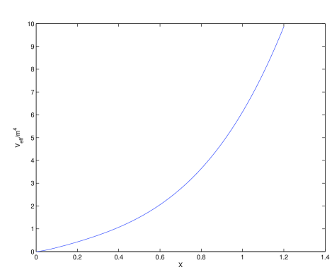
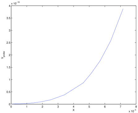
Figure 1: The scalar effective potential in the deformed CFT with $M=0$ and $\beta=-\pi/4$ (left) and the probe potential in the deformed AdS with $\alpha=0$ (right)

The solution of the equations of motion depends on boundary conditions related to the asymptotic behavior of the field $\lambda$. The numerical analysis was done for $(\mathcal{M},\mathcal{K})=(1,0)$. As discussed at the end of 3.1, the value of $\mathcal{K}$ remains undetermined in the supergravity analysis (one expects $\mathcal{K}$, which corresponds to the gluino condensate in the CFT, to be of order unity in units of $m^{3}$). Fortunately, the qualitative behavior of the potential does not seem to depend much on this number. Allowing other values for the parameters ($\mathcal{K}>0$) does not change the qualitative features shown in figure 1.

4 Conclusions

We have calculated the effective potential of the $\mathcal{N}=0^{*}$ theory and shown that 1-loop corrections make the potential stable in specific directions that are flat at tree level (i.e. flat in the unmodified $\mathcal{N}=4$ SYM theory). Note that although the gauge symmetry and the global R-symmetry restrict the general form of the potential, they do not fix it completely and there remain unexplored directions which were flat in $\mathcal{N}=4$ SYM.

It is interesting that the scalar potential we found in the $\mathcal{N}=0^{*}$ theory is qualitatively similar to the probe potential in its supergravity dual, although their ranges of validity do not coincide.

We have seen some indications that the vacuum of the $\mathcal{N}=0^{*}$ theory is at $\left\langle\phi^{i}\right\rangle=0$, implying that both the gauge symmetry and the R-symmetry remain unbroken. The location of the vacuum depends on the sign of the parameters $M_{1}^{2}$ and $M_{2}^{2}$ introduced in (11). In subsection 2.2 we gave arguments why these parameters should be positive, but they are not a proof, since they fail at low energies (where the theory becomes strongly coupled and the perturbative description fails). The brane probe potential in the supergravity approximation also indicates the same conclusion (a stable symmetric vacuum). However, it too fails in the interior of the AdS, implying the approximation breaks down and should not be trusted for small $X$.

The failure of the supergravity approximation in the interior of the AdS is a hint for stringy physics in this area. The true string vacuum dual to $\mathcal{N}=0^{*}$ is likely to be described by some extended brane configuration, analogous to the configurations found by Polchinski and Strassler [10] for the string dual of the $\mathcal{N}=1^{*}$ theory. Among its other advantages, knowing the full string background should allow one to calculate the value of the parameter $\mathcal{K}$ (introduced in (20)), thus picking the right solution asymptotically for a given $\mathcal{M}$. It is also interesting to see if the qualitative similarity between the effective potential in the $\mathcal{N}=0^{*}$ theory and the probe potential in its supergravity dual, as depicted in Figure 1, will abide outside the supergravity approximation.

References

• [1] J.Β M. Maldacena, β€œThe large $N$ limit of superconformal field theories and supergravity,” Adv. Theor. Math. Phys. 2 (1998) 231–252, hep-th/9711200.
• [2] E.Β Witten, β€œAnti-de sitter space and holography,” Adv. Theor. Math. Phys. 2 (1998) 253–291, hep-th/9802150.
• [3] S.Β S. Gubser, I.Β R. Klebanov, and A.Β M. Polyakov, β€œGauge theory correlators from non-critical string theory,” Phys. Lett. B428 (1998) 105–114, hep-th/9802109.
• [4] O.Β Aharony, S.Β S. Gubser, J.Β M. Maldacena, H.Β Ooguri, and Y.Β Oz, β€œLarge $N$ field theories, string theory and gravity,” Phys. Rept. 323 (2000) 183–386, hep-th/9905111.
• [5] O.Β Aharony, β€œThe non-AdS/non-CFT correspondence, or three different paths to QCD,” hep-th/0212193.
• [6] J.Β Babington, D.Β E. Crooks, and N.Β J. Evans, β€œA stable supergravity dual of non-supersymmetric glue,” Phys. Rev. D67 (2003) 066007, hep-th/0210068.
• [7] S.Β R. Coleman and E.Β Weinberg, β€œRadiative corrections as the origin of spontaneous symmetry breaking,” Phys. Rev. D7 (1973) 1888–1910.
• [8] A.Β P. Prudnikov, Y.Β A. Brychkov, and O.Β I. Marichkev, Integrals and Series, vol.Β 1, p.Β 617. Gordon and Breach Science Publishers, New York, 1998.
• [9] L.Β Girardello, M.Β Petrini, M.Β Porrati, and A.Β Zaffaroni, β€œThe supergravity dual of N=1 super Yang-Mills theory,” Nucl. Phys. B569 (2000) 451–469, hep-th/9909047.
• [10] J.Β Polchinski and M.Β J. Strassler, β€œThe string dual of a confining four-dimensional gauge theory,” hep-th/0003136.