We discuss the AdS/CFT duality from the perspective of integrable systems and establish a direct relationship between the dimension of single trace local operators composed of two types of scalar fields in ${\cal N}=4$ super Yang-Mills and the energy of their dual semiclassical string states in $AdS_{5}\times S^{5}$. The anomalous dimensions can be computed using a set of Bethe equations, which for “long” operators reduces to a Riemann-Hilbert problem. We develop a unified approach to the long wavelength Bethe equations, the classical ferromagnet and the classical string solutions in the $SU(2)$ sector and present a general solution, governed by complex curves endowed with meromorphic differentials with integer periods. Using this solution we compute the anomalous dimensions of these long operators up to two loops and demonstrate that they agree with string-theory predictions.

1 Introduction

Gauge/string duality is an old and fascinating subject that appears in a variety of situations [1]. This subject encompasses a large circle of ideas, the most promising of which, perhaps, is the relationship between strings and planar diagrams in the large-$N$ limit [2]. A well known example of such a duality is the matrix model description of two-dimensional quantum gravity and noncritical strings [3, 4]. Matrix models [5], together with two-dimensional QCD [6], are two instructive examples in which the large-$N$ limit is solvable.

A much more complicated case of this large-$N$ duality is the AdS/CFT correspondence, an asserted equivalence of a four-dimensional gauge theory with ${\cal N}=4$ supersymmetry and type IIB string theory on the product space $AdS_{5}\times S_{5}$. Among other predictions, the AdS/CFT conjecture relates the dimensions of gauge-invariant operators with the energies of particular closed string states propagating in the $AdS_{5}\times S_{5}$ background [7, 8, 9]. At present, it has only been possible to test this conjecture for a limited class of operators. The reason, of course, is that the string calculations are trustworthy for large ’t Hooft coupling $\lambda=g^{2}N$, while the gauge theory calculations are reliable if $\lambda$ is small.

There are two basic sets of operators which get around this mismatch of the coupling strength. The first set contains the chiral primary operators and their descendants. Here one may rely on nonrenormalization theorems to test directly the correspondence [7, 8, 9]. The second set consists of operators with large global charges, which are dual to semiclassical string states. An example of this operator type are the so called BMN operators [10]. Here, one starts with a chiral primary made up of a large number of complex scalar fields ($\,{\rm Tr}\,{\mbox{\boldmath$\Phi$}}^{L}$ for $L\gg 1$), adds to the operator a handful of “impurities”, which can either be other scalar fields or covariant derivatives acting on the $\Phi$ fields, and then sums over the positions of the impurities weighted by some phases. On a superficial level, the dual closed string can be visualized as a chain of scalar fields inside a trace, where the impurities on the chain correspond to excitations of the string. The precise AdS dual of the chiral primary is a point-like string orbiting a geodesic of $S^{5}$ with angular momentum $L$, large enough for the classical approximation to be accurate [11]. The nearby spacetime of the string trajectory has a plane wave geometry in which the world-sheet string action in the light-cone gauge can be formulated as an infinite set of massive oscillators [12, 13]. Therefore a direct comparison can be made between the anomalous dimensions of the perturbative gauge theory [10, 14, 15] and the energies of the string oscillations in the plane wave.

Since the BMN operators are assumed to have a small number of impurities, the strings dual to these operators are almost pointlike. Once the string has significant stretching, the exact string spectrum is unknown. Nevertheless, following [11], a large number of classical string solutions in $AdS_{5}\times S^{5}$ have been constructed [16, 17, 18, 19, 20, 21, 22, 23, 24, 25]. These string configurations are described by solitons of the world-sheet sigma-model, all of which have large actions and therefore correspond to semiclassical states that are high in the energy spectrum of the string. A potential difficulty in comparing string solitons to the supersymmetric Yang-Mills (SYM) operators is that the operators are necessarily large, i. e. they must contain many constituent fields in order to carry large quantum numbers. The computation of the anomalous dimension for large operators, even at one loop, is hindered by operator mixing which lifts the degeneracy of the classical scaling dimensions. The degeneracy grows exponentially with the size of the operators and the mixing becomes more and more complicated. Fortunately, the mixing matrix can be identified with the Hamiltonian of an integrable spin chain [27, 28, 29]. One can then use powerful techniques of the algebraic Bethe ansatz [30] (see the up to date formulation of this method in [31]) to diagonalize the mixing matrix and to compute the anomalous dimensions. Explicit calculations have led to a remarkable agreement with string theory predictions in several cases [32, 33, 24, 34].

Much of the recent progress focused on single trace operators composed of two types of complex scalar fields, ${\mbox{\boldmath$\Phi$}}_{1}$ and ${\mbox{\boldmath$\Phi$}}_{2}$, of the form

$$\begin{array}[]{c}{\rm Tr}\left({\mbox{\boldmath$\Phi$}}_{1}{\mbox{\boldmath$\Phi$}}_{1}{\mbox{\boldmath$\Phi$}}_{1}{\mbox{\boldmath$\Phi$}}_{2}{\mbox{\boldmath$\Phi$}}_{2}{\mbox{\boldmath$\Phi$}}_{1}{\mbox{\boldmath$\Phi$}}_{2}{\mbox{\boldmath$\Phi$}}_{2}{\mbox{\boldmath$\Phi$}}_{1}{\mbox{\boldmath$\Phi$}}_{1}{\mbox{\boldmath$\Phi$}}_{1}{\mbox{\boldmath$\Phi$}}_{2}\ldots\right)\,.\end{array}$$ (1.1)

It was shown in [27] that the one loop dilatation generator when acting on operators of this type is equivalent to the Hamiltonian of the XXX Heisenberg spin chain. Hence, we will call operators with the form in (1.1) XXX operators. These operators are naturally identified with the states of the spin chain by associating, say, ${\mbox{\boldmath$\Phi$}}_{1}$ with up spins and ${\mbox{\boldmath$\Phi$}}_{2}$ with down spins. For instance, the operator (1.1) is mapped to the state

$$\left|\uparrow\uparrow\uparrow\downarrow\downarrow\uparrow\downarrow\downarrow\uparrow\uparrow\uparrow\downarrow\ldots\right\rangle\in\left({\bf C}^{2}\right)^{\otimes L}.$$

The one loop dilatation operator of ${\cal N}=4$ planar SYM theory was found in [27], and its two loop correction was proposed in [38]. It has the following form in this basis

$$\begin{array}[]{c}\hat{D}=L+\frac{\lambda}{16\pi^{2}}\sum_{l=1}^{L}\left(1-{{{\mathchoice{\hbox{$\displaystyle\sigma$}}{\hbox{$\textstyle\sigma$}}{\hbox{$\scriptstyle\sigma$}}{\hbox{$\scriptscriptstyle\sigma$}}}}}_{l}\cdot{{{\mathchoice{\hbox{$\displaystyle\sigma$}}{\hbox{$\textstyle\sigma$}}{\hbox{$\scriptstyle\sigma$}}{\hbox{$\scriptscriptstyle\sigma$}}}}}_{l+1}\right)+\\ \left(\frac{\lambda}{16\pi^{2}}\right)^{2}\ \sum_{l=1}^{L}\left(\left(1-{{{\mathchoice{\hbox{$\displaystyle\sigma$}}{\hbox{$\textstyle\sigma$}}{\hbox{$\scriptstyle\sigma$}}{\hbox{$\scriptscriptstyle\sigma$}}}}}_{l}\cdot{{{\mathchoice{\hbox{$\displaystyle\sigma$}}{\hbox{$\textstyle\sigma$}}{\hbox{$\scriptstyle\sigma$}}{\hbox{$\scriptscriptstyle\sigma$}}}}}_{l+2}\right)-4\left(1-{{{\mathchoice{\hbox{$\displaystyle\sigma$}}{\hbox{$\textstyle\sigma$}}{\hbox{$\scriptstyle\sigma$}}{\hbox{$\scriptscriptstyle\sigma$}}}}}_{l}\cdot{{{\mathchoice{\hbox{$\displaystyle\sigma$}}{\hbox{$\textstyle\sigma$}}{\hbox{$\scriptstyle\sigma$}}{\hbox{$\scriptscriptstyle\sigma$}}}}}_{l+1}\right)\right)+O(\lambda^{3}),\end{array}$$ (1.2)

where ${{\mathchoice{\hbox{$\displaystyle\sigma$}}{\hbox{$\textstyle\sigma$}}{\hbox{$\scriptstyle\sigma$}}{\hbox{$\scriptscriptstyle\sigma$}}}}_{l}$ are the Pauli matrices which act on the spin at the $l^{\rm th}$ site of the chain. The dilatation operator is not diagonal in the basis of monomials and mixes simple operators of type (1.1). It can be diagonalized, at one loop (first line in (1.2)) by using the Bethe ansatz technique [30].

On the string side, restriction to XXX operators corresponds to a string moving on the subspace $S^{3}\subset S^{5}$ and localized to the center of $AdS_{5}$. In [35] it was shown how to directly compare the equations of motion for a classical spin chain with the string sigma model equations of motion by taking a “nonrelativistic” limit of the effective coupling. The classical chain naturally corresponds to the long wave-length limit of the quantum chain [36, 37], which is precisely what was considered in [32, 33, 24].

An obvious question is how the integrability of the spin chain relates to integrability of the sigma model. There is a body of evidence that the integrability of the mixing matrix for the XXX operators is not an accidental symmetry of the one loop approximation. The XXX operators mix only with themselves to all orders in pertubation theory and in this subsector the integrability definitely extends to two loops [38], to three loops [38, 39, 40, 41], and possibly to higher loops [42]. On top of this, it has been verified that the superstring sigma-model in $AdS_{5}\times S^{5}$ is classically integrable [43, 44]. Furthermore, it was shown how solutions on the sigma model reduce to a classically integrable mechanics, allowing one to explicitly solve for the string motion [23, 25]. The integrable structures on the two sides of the AdS/CFT correspondence should be related in some fashion. On an algebraic level, the relation among the integrals of motion was discussed in [45]. Subsequently, Arutyunov and Staudacher were able to make a direct comparison between certain string solitons and large XXX operators in SYM, showing that the entire integrable hierarchy matches in the small coupling limit [46]. This matching of hierachies has also been extended to certain classical solutions of the $SU(3)$ chain [47].

The main goal of this paper is to develop a unified approach to the Bethe ansatz, string solitons and the weak-coupling “non-relativistic” reduction of the sigma-model. We will discuss in detail mainly the XXX subsector, though we will also mention a set of string solutions that are not dual to this class of operators.

In comparing perturbative gauge theory results to string theory predictions, it is important to note that gauge theory and string theory compute different expansions for the anomalous dimension. The string calculations are accurate when both the bare dimension of the operator, $L$, and the ’t Hooft coupling $\lambda$ are large, but the ratio $\lambda/L^{2}$ is finite. Since the relevant parameter is $\lambda/L^{2}$, it is possible to consider strong coupling on the string side and still have $\lambda/L^{2}$ small. One might then expect to make a direct comparison to perturbative gauge theory.

However, it was argued by Serban and Staudacher [42] that nonperturbative terms could complicate the situation. These authors showed that a particular long range spin chain would reproduce the two-loop and three-loop dilatation operators of [38, 39, 40] if one identifies $\lambda/L^{2}$ with a parameter of the spin chain. They then went on to show that the operators dual to a folded and a circular string match at two-loops, but fail to do so at three-loops.

But even two-loop matching is mysterious. On general grounds, the classical string predicts the dimension of the operator to be $\sqrt{\lambda}F(\lambda/L^{2})$ with some function $F(\lambda/L^{2})=L/\sqrt{\lambda}+...$. Any stringy nonperturbative contribution to the dimension should be of the form

$$\begin{array}[]{c}f(\lambda/L^{2})\exp(-\sqrt{\lambda}g(\lambda/L^{2})).\end{array}$$ (1.3)

Of course this term and others like it cannot be in general separated in the same exponential form on the gauge side, but just as an illustration let us momentarily take them seriously, in which case they can be perturbative in the gauge theory. In order to have a sensible contribution to perturbative gauge theory, we should require that the Taylor expansion of $f(\lambda/L^{2})$ and $g(\lambda/L^{2})$ about $\lambda/L^{2}=0$ have integer and half integer powers respectively. If the lowest power of $g$ is $n\leq-{\textstyle{1\over 2}}$, then there would be an exponential suppression in $L$ for all orders of $\lambda$ and (1.3) would not contribute to any order in perturbation theory in the large $L$ limit. However, if the first power is $n={\textstyle{1\over 2}}$, then (1.3) can affect the perturbative expansion in the large $L$ limit. However, (1.3) should not contribute to the bare dimension of the operator, requiring that $f(0)=0$. Hence, the term that can affect the perturbative gauge theory expansion at the lowest possible order would have the form $\sim(\lambda/L^{2})(1-a\lambda/L+{1\over 2}a^{2}\lambda^{2}/2L^{2}+...)$. The lowest term in this expansion is a one-loop term, but it is suppressed by a factor of $L$ from the classical string contribution so it can be ignored. The second term is a two loop term which scales like the classical contribution and so its existence would affect the two loop gauge contribution. The third term is a three-loop term which does not even have perturbative BMN scaling. What is puzzling is that the breakdown described here seems to take place at one loop higher. In fact it was shown in [42] that assuming that perturbative Yang-Mills is described by an Inozemtsev chain [48], perturbative BMN scaling breaks down at four loops.

We will demonstrate that indeed the Riemann-Hilbert problem on the string theory side immediately reproduces one and two loops in gauge theory. We do not study the three-loop reduction of the sigma-model in this paper, but are planning ot return to this question in the near future.

In what follows we will consider generic solutions to the class of so called finite-gap potentials. These solutions are directly related to algebraic geometry on finite genus Riemann surfaces. From the point of view of the Bethe equations, this corresponds to the Bethe roots condensing onto a finite number of “supports” in the complex plane. Such geometric objects have been previously used in SUSY gauge theories. For example, the Seiberg-Witten solution to ${\cal N}=2$ SYM is formulated in terms of the geometry of curves [49] which in turn can be nicely translated into the language of integrable systems [50] in a class closely related to those considered below. In the ${\cal N}=2$ case the trajectories of the integrable model correspond to BPS states while in the ${\cal N}=4$ case they correspond to composite operators. This relationship deserves further investigation.

We should mention that integrable spin chains arise in large-$N$ QCD [51, 52, 53, 54, 55] (the quasiclassical solutions to the Bethe anzatz equations were considered in this context in [56, 57]) and in less supersymmetric cousins of ${\cal N}=4$ SYM [58, 59, 60, 61, 62]. Potential relevance of the XXZ spin chain for gauge/string theory duality was discussed in [63].

In sect. 2 we review the Bethe ansatz and discuss the reduction of the Bethe equations in the scaling limit to integral equations, similar to those found for matrix models. In sect. 3 we construct the generic solution of this Bethe ansatz integral equation describing the one-loop ${\cal N}=4$ Yang-Mills theory and then generalize it to two loops. Sect. 4 is devoted to classical integrability: we show that the solutions of the Bethe equations in the scaling limit are in one-to-one correspondence with the finite-gap solutions of the weak-coupling sigma-model at one loop in the gauge coupling. Moreover, we then derive the classical counterpart of the Bethe equations in the string sigma-model and discuss the general underlying geometry of the sigma-model solutions. In particular, we find that the resolvent of the Bethe roots, which is the generator of the higher charges of the integrable system, is closely related to the quasi-momentum of the sigma-model and that the latter reduces to the former in the limit of zero coupling, i.e. at one loop. At two loops, the precise map between the sigma-model and the spin chain involves redefinition of the spectral parameter. In section 5 we apply the general formalism of sections 3 and 4 to concrete examples. We obtain some new solutions as well as rederive known results to illustrate the general method. Included in these examples are general rational solutions where the Bethe roots condense onto one cut. We also consider a sigma-model solution which corresponds to a “pulsating string” and show that the quasi-momentum reduces to the resolvent of a particular solution of the $SO(6)$ chain in the scaling limit. In sect. 6 we present conclusions and speculations. Some technical issues are presented in Appendices.

2 The Bethe Ansatz

Here we will derive the Bethe-type equations for the diagonalisation of the one-loop dilaton operator. The generalisation to two loops will be presented at the end of the section 3.

If we assign $R$-charges $(1,0)$ and $(0,1)$ to the complex scalars ${\mbox{\boldmath$\Phi$}}_{1}$ and ${\mbox{\boldmath$\Phi$}}_{2}$, the eigenstates of the Heisenberg Hamiltonian with $J$ down spins out of $L$ total spins correspond to conformal operators with $R$-charges $(J_{1},J_{2})=(L-J,J)$:

$$\begin{array}[]{c}{\cal O}={\rm Tr}\left({\mbox{\boldmath$\Phi$}}_{1}^{L-J}{\mbox{\boldmath$\Phi$}}_{2}^{J}+{\rm permutations}\right).\end{array}$$ (2.1)

Each eigenstate of the dilatation operator (1.2) describes a collection of $J$ interacting spin waves with rapidities $u_{1},\ldots,u_{J}$. The spin waves attract and can form bound states, so the rapidities are in general complex. The eigenstates form representations of $SU(2)$ generated by the total spin which commutes with the Hamiltonian. The highest weight in each $SU(2)$ representation can be constructed with the help of the algebraic Bethe ansatz [31] and is completely characterized by a set of rapidities. These rapidities must be distinct complex numbers, are either real or form complex conjugate pairs, and satisfy a set of algebraic Bethe equations.

The integrable structure of the Heisenberg spin chain is encoded in the transfer matrix (see, for example, [31] and references therein) defined as

$$\begin{array}[]{c}\hat{T}(u)={\rm Tr}\,\left[\left(u+\frac{i}{2}\,{{{\mathchoice{\hbox{$\displaystyle\sigma$}}{\hbox{$\textstyle\sigma$}}{\hbox{$\scriptstyle\sigma$}}{\hbox{$\scriptscriptstyle\sigma$}}}}}_{L}\otimes{{{\mathchoice{\hbox{$\displaystyle\sigma$}}{\hbox{$\textstyle\sigma$}}{\hbox{$\scriptstyle\sigma$}}{\hbox{$\scriptscriptstyle\sigma$}}}}}\right)\ldots\left(u+\frac{i}{2}\,{{{\mathchoice{\hbox{$\displaystyle\sigma$}}{\hbox{$\textstyle\sigma$}}{\hbox{$\scriptstyle\sigma$}}{\hbox{$\scriptscriptstyle\sigma$}}}}}_{1}\otimes{{{\mathchoice{\hbox{$\displaystyle\sigma$}}{\hbox{$\textstyle\sigma$}}{\hbox{$\scriptstyle\sigma$}}{\hbox{$\scriptscriptstyle\sigma$}}}}}\right)\right].\end{array}$$ (2.2)

The Pauli matrices without a superscript $\textstyle\sigma$ act in a two-dimensional auxiliary space, and tracing in (2.2) over the auxiliary space leaves an operator in the Hilbert space of the spin chain. The transfer matrices at different values of the spectral parameter $u$ commute and therefore generate an infinite set of conserved charges in involution . The Taylor expansion of the transfer matrix at $u=i/2$ generates mutually commuting local charges:

$$\begin{array}[]{c}\hat{T}(u)=\left(u+\frac{i}{2}\right)^{L}\par\hat{U}\exp\left[i\sum_{n=1}^{\infty}\frac{1}{n}\,\left(u-\frac{i}{2}\right)^{n}\hat{Q}_{n}\right],\end{array}$$ (2.3)

where $\hat{U}={\,\rm e}\,^{i\hat{P}}$ is the shift operator that generates translations by one site. The first charge from the sum in the exponent of (2.3) is proportional to the one-loop dilatation operator (1.2): $\hat{D}=L+{\lambda\over 8\pi^{2}}\,\hat{Q}_{1}+O(\lambda^{2})$. The Laurent expansion of (2.2) at $u=\infty$ (before taking the trace over the auxiliary matrices) produces the total spin and non-local Yangian charges (see the recent discussion of Yangian symmetry and its relation to Yang-Mills theory in [45]).

The Bethe ansatz diagonalizes the whole tranfer matrix,

$$\begin{array}[]{c}\hat{T}(u)\left|u_{1}\ldots u_{J}\right\rangle=T(u)\left|u_{1}\ldots u_{J}\right\rangle,\end{array}$$ (2.4)

giving eigenvectors that depend on $J$ rapidities and whose eigenvalues are

$$\begin{array}[]{c}T(u)=\left(u+\frac{i}{2}\right)^{L}\prod_{k=1}^{J}\frac{u-u_{k}-i}{u-u_{k}}+\left(u-\frac{i}{2}\right)^{L}\prod_{k=1}^{J}\frac{u-u_{k}+i}{u-u_{k}}\end{array}$$ (2.5)

The second term does not affect the local charges (2.3) as it is multiplied by a huge power of $u-i/2$.

The Bethe equations are obtained from (2.5) by simply noting that the function $T(u)$, by construction, must be a polynomial of degree $L$, or for $L\to\infty$ an entire analytic function of $u$. Hence it has no poles at any $u=u_{j}$, and this immediately leads to the $J$ conditions

$$\begin{array}[]{c}\left(u_{j}+i/2\over u_{j}-i/2\right)^{L}=\prod_{k=1(k\neq j)}^{J}{u_{j}-u_{k}+i\over u_{j}-u_{k}-i},\end{array}$$ (2.6)

which are in fact the Bethe equations.

These Bethe equations also represent periodicity conditions for the wave function and can be written in the logarithmic form as

$$\begin{array}[]{c}L\log\left(u_{j}+i/2\over u_{j}-i/2\right)=\sum_{k=1(k\neq j)}^{J}\log{u_{j}-u_{k}+i\over u_{j}-u_{k}-i}-2\pi in_{j}.\end{array}$$ (2.7)

The mode numbers $n_{j}$ are arbitrary integers. The cyclicity of the trace in the operators of ${\cal N}=4$ supersymmetric Yang-Mills requires that

$$\begin{array}[]{c}{\,\rm e}\,^{iP}=\prod_{j=1}^{J}{u_{j}+i/2\over u_{j}-i/2}=1,\end{array}$$ (2.8)

which is the quantization condition on the total momentum: ${p\over 2\pi}\in\vbox{\hbox{\numbers\hbox to0.0pt{\hbox to0.0pt{Z\hss}\kern 0.8pt\vrule height=8.0pt,width=0.5pt,depth=-5.9pt\hss}\kern 2.2pt\hbox to0.0pt{Z\hss}\kern 6.0pt\vrule height=2.0pt,width=0.5pt,depth=0.1pt\kern 1.0pt}}$. The energy of the solution gives the anomalous dimension $\gamma$ of the corresponding operator in Yang-Mills theory [27],

$$\begin{array}[]{c}\gamma={\lambda\over 8\pi^{2}}\sum_{j=1}^{J}{1\over u_{j}^{2}+1/4}\,.\end{array}$$ (2.9)

In the scaling limit of large operators where $L\to\infty$, all Bethe roots are of order $u_{j}\sim L$. By rescaling $u_{j}=Lx_{j}$ we can then write eq. (2.7) in the form

$$\begin{array}[]{c}{1\over x_{j}}={2\over L}\sum_{k=1(k\neq j)}^{J}{1\over x_{j}-x_{k}}-2\pi n_{j}.\end{array}$$ (2.10)

Let us consider the situation with a finite number of different mode numbers $n_{j}$, and assume that the number of Bethe roots with the same mode number is of order $L$. The roots with mode number $n_{k}$ are centered roughly around the point $x=1/(2\pi n_{k})$, with a typical separation between adjacent roots of order $\Delta x\sim 1/L$. Hence, roots with the same mode number form a continuous contour in the complex plane in the scaling limit $L\rightarrow\infty$.

Equations (2.10) are very similar to the saddle point equations for matrix models (apart from the last term, to be discussed below), where the Bethe roots are the analogs of the matrix eigenvalues. Just like for matrix eigenvalues, one can characterize the distribution of Bethe roots by the density

$$\begin{array}[]{c}\rho(x)=\frac{1}{L}\sum_{j}\delta(x-x_{j})\end{array}$$ (2.11)

or by the resolvent

$$\begin{array}[]{c}G(x)={1\over L}\sum_{j=1}^{J}{1\over x-x_{j}}=\int_{\bf C}{d\xi\,\rho(\xi)\over x-\xi}\,.\end{array}$$ (2.12)

The density is non-zero on a set of contours ${\bf C}$ in the complex plane which in general consists of several non-overlapping cuts, ${\bf C}={\bf C}_{1}\cup\ldots\cup{\bf C}_{K}$, where the $l^{\rm th}$ cut ${\bf C}_{l}=(a_{l},b_{l})$ represents roots with mode number $n_{l}$. Though we will assume that the number of cuts is finite, this requirement can certainly be relaxed. We will return to this point in the discussion of classical integrability of the string sigma-model. As follows from its definition, the resolvent is an analytic function on the complex plane with cuts. Asymptotically it has the form

$$\begin{array}[]{c}G(x)=\frac{\alpha}{x}+\dots\,,~{}~{}~{}~{}~{}(x\rightarrow\infty),\end{array}$$ (2.13)

which reflects the normalization condition for the density

$$\begin{array}[]{c}\int_{\bf C}d\xi\,\rho(\xi)=\alpha,\end{array}$$ (2.14)

where $\alpha=J/L$ is the filling fraction, the fraction of down spins in the Bethe state. Strictly speaking, Bethe states only make sense for $\alpha\leq{\textstyle{1\over 2}}$, but it was observed in a number of examples [32, 33, 24] that solutions of the Bethe equations can be analytically continued past $\alpha={\textstyle{1\over 2}}$. We will clarify the meaning of this analytic continuation in sections  3 and 5.4. The analytic continuation is always possible and the analytically continued solution corresponds to some Bethe state with $\alpha$ replaced by $1-\alpha$. Since replacing $\alpha$ with $1-\alpha$ is equivalent to interchanging ${\mbox{\boldmath$\Phi$}}_{1}$ and ${\mbox{\boldmath$\Phi$}}_{2}$ in the operator ${\rm Tr}({\mbox{\boldmath$\Phi$}}_{1}^{J_{1}}{\mbox{\boldmath$\Phi$}}_{2}^{J_{2}}+\ldots)$, $J_{1}=L-J$, $J_{2}=J$, the resulting state has essentially the same charges. We thus allow for $0\leq\alpha\leq 1$ and regard charges of the states with $\alpha$ and $1-\alpha$ as equal.

The scaling limit of the Bethe equations (2.10) can be rewritten as an integral equation for the density,

$$\begin{array}[]{c}G(x+i0)+G(x-i0)=2{-\!\!\!\!\!\!\int}_{{\bf C}}{d\xi\,\rho(\xi)\over x-\xi}={1\over x}+2\pi n_{l},\ \ \ x\in{\bf C}_{l}\end{array}$$ (2.15)

The momentum condition (2.8) after rescaling turns into

$$\begin{array}[]{c}P={1\over L}\sum_{j=1}^{J}{1\over x_{j}}=2\pi m,\ \ \ \ m\in\vbox{\hbox{\numbers\hbox to0.0pt{\hbox to0.0pt{Z\hss}\kern 0.8pt\vrule height=8.0pt,width=0.5pt,depth=-5.9pt\hss}\kern 2.2pt\hbox to0.0pt{Z\hss}\kern 6.0pt\vrule height=2.0pt,width=0.5pt,depth=0.1pt\kern 1.0pt}}\end{array}$$ (2.16)

or, taking into account the Bethe equations (2.10) and (2.15),

$$\begin{array}[]{c}-{1\over 2\pi i}\oint_{{\bf C}}{G(x)dx\over x}=\sum_{k=1}^{K}\int_{{\bf C}_{k}}{\rho(x)dx\over x}=2\pi\sum_{l=1}^{K}n_{l}\int_{{\bf C}_{l}}\rho(x)dx=2\pi m,\ \ \ \ \ n_{l},m\in\vbox{\hbox{\numbers\hbox to0.0pt{\hbox to0.0pt{Z\hss}\kern 0.8pt\vrule height=8.0pt,width=0.5pt,depth=-5.9pt\hss}\kern 2.2pt\hbox to0.0pt{Z\hss}\kern 6.0pt\vrule height=2.0pt,width=0.5pt,depth=0.1pt\kern 1.0pt}}.\end{array}$$ (2.17)

For the anomalous dimension (2.9) we obtain in the scaling limit

$$\begin{array}[]{c}\gamma={\lambda\over 8\pi^{2}L}\int dx\,\frac{\rho(x)}{x^{2}}=-{\lambda\over 8\pi^{2}L}\oint_{\bf C}{dx\over 2\pi i\,x^{2}}\,G(x)\end{array}$$ (2.18)

Rescaling the spectral parameter $u=Lx+i/2$ in the eigenvalue of the transfer matrix and dropping the second irrelevant term in (2.5) we find in the limit $L\rightarrow\infty$:

$$\begin{array}[]{c}\frac{T(Lx+i/2)}{\left(Lx+i/2\right)^{L}}=\exp\left(-\frac{i}{L}\sum_{j}\frac{1}{x-x_{j}}\right)\end{array}$$ (2.19)

Comparing with (2.3), we see that the resolvent (2.12) is the generating function of local charges in the scaling limit [46, 24]. Obviously, the first two coefficients in its Taylor expansion are the total momentum and the energy.

Our derivation of the integral equation for the density of Bethe roots rested on the assumption that the right-hand side of the Bethe equations can be expanded in powers of $1/(u_{j}-u_{k})$. This is not always true. The assumption breaks down if the distance between nearby roots $u_{j}-u_{k}$ approaches $i$. Some solutions of the Bethe equations are known to have roots separated exactly by $i$ in the thermodynamic limit. The roots form arrays with equidistant separation: $u_{j}=u_{0}+i\ j$. Such arrays are usually referred to as “strings” [31] and survive the thermodynamic limit due to the chain cancellation of dangerous terms in the sum entering eq. (2.7). It is certainly possible to have large strings composed of a macroscopic number of roots. The density will then have constant pieces with a flat distribution, $\rho(x)=1$. Such condensates of Bethe roots necessarily have tails with smaller density. Condensates thus can be viewed as extra logarithmic cuts in the complex plane that connect pairs of the original contours ${\bf C}_{l}$ (the situation is identical to that arising in multicolor 2D Yang-Mills theory on the sphere [64]). The resolvent experiences a jump by $2\pi$ across any of these extra cuts and is no longer a single-valued function. The integral equation (2.15) stays the same, but we have extra conditions on its solution as it crosses these logarithmic cuts.

The solution of the Bethe equations with a condensate along the imaginary axis is one of the examples in which the agreement between the anomalous dimension and the energy of a string soliton was first observed [32]. In that example, however, the roots were separated not by $i$, but by a half-integer interval $i/2$, and the condensate had the density $\rho(x)=2$. We do not see any reason why strings of an arbitrary integral density cannot appear: for the distribution of roots $u_{j}=u_{0}+i\ {j\over m}$, where $m$ is any positive integer, the same cancellation mechanism is at work [65]. Though these denser strings apparently have never been discussed in the literature on the Bethe Ansatz, their existence is quite natural, at least in the long chain limit considered here. Another argument in favor of condensates of an arbitrary density is that solutions $\rho(x)=2m$ are necessary to match the string theory predictions, where the integer $m$ plays the role of the winding number.

To summarize, Bethe roots in the scaling limit are continuously distributed on a collection of contours ${\bf C}_{l}$ in the complex plane and may also form condensates, which connect pairs of contours and on which the density takes constant integer values. The density of roots $\rho(x)dx$ is real, positive and is normalized to the filling fraction $\alpha$. It must also be symmetric under complex conjugation of $x$. The density of Bethe roots satisfies an integral equation (2.15) which holds on each of the ${\bf C}_{l}$’s. All possible solutions to the Bethe equations in the scaling limit are thus parameterized by specifying mode numbers $n_{l}$ associated with contours ${\bf C}_{l}$ and integer densitities of condensates $m_{l}$. Once these numbers are specified we can solve the integral equation, at least in principle, and find the density. We will see, however, that there is a symmetry that transforms different sets of integers $(n_{l},m_{l})$ into each other so that solutions with different sets of $m$’s and $n$’s lead to the same resolvent.

3 General solution

In this section we first construct the general solution of equation (2.15) and then consider corrections to this solution arising from the two-loop contributions in SYM theory.

3.1 General one-loop solution

Following the procedure proposed in [36] we introduce

$$\begin{array}[]{c}p(x)=G(x)-{1\over 2x},\end{array}$$ (3.1)

which we shall call the quasi-momentum for reasons explained in the next section, and rewrite (2.15) in the form of a Riemann-Hilbert problem defining the analytic function $p(x)$ from its discontinuities

$$\begin{array}[]{c}p(x+i0)+p(x-i0)=2\pi n_{i},\ \ \ \ \ \ \ \ x\in{\bf C}_{i}\end{array}$$ (3.2)

on every cut ${\bf C}_{i}$. Equation (3.2) together with relation (3.1) are very similar to the corresponding equations arising in the quasiclassical computation of matrix integrals. The main difference is the presence of the mode numbers $n_{j}$, which are different on the different eigenvalue supports. Therefore, unless there is only one cut, the resolvent $G(x)$ and the quasimomentum $p(x)$ are not algebraic functions, i.e. in contrast to a very similar equation found for the one matrix model (see e.g. [66]) and even the more complicated situation of the two-matrix model [67], the resolvent and quasimomentum can not be determined by solving a polynomial equation .

It follows nevertheless from (3.2) that $p(x)$ is a double-valued function of $x$. It must be single-valued on the physical sheet of its Riemann surface, which is a complex plane with cuts ${\bf C}_{j}$. The only singularities of $p(x)$ are two poles at $x=0$ on the two sheets of the Riemann surface. The pole on the physical sheet should cancel in $G(x)$, which by definition should be regular at zero. In other words, $p(x)=\int^{x}dp$ is an Abelian integral for the meromorphic differential $dp$, which has two double-poles at $x=0$ and integer periods on a hyperelliptic curve $\Sigma$. Let

$$\begin{array}[]{c}\Sigma:\ \ \ \ y^{2}=R_{2K}(x)=x^{2K}+r_{1}x^{2K-1}+\dots+r_{2K}=\prod_{j=1}^{2K}(x-{\rm x}_{j})\end{array}$$ (3.3)

where the product is taken over the end-points of all $K$ cuts ${\bf C}_{l}\in{\bf C}$. We should also impose the reality constraint on the whole solution such that the branch-points of every cut have complex conjugated coordinates, ${\rm x}_{2j}={\rm x}_{2j+1}^{*}$. The other possiblity is that some ${\rm x}_{k}$’s are real, but it is never realized in the present case, although solutions with real cuts do exist for spin $s=-{\textstyle{1\over 2}}$ chains [33] and are relevant for SYM duals of strings with nonzero angular momentum in $AdS_{5}$ [16]. In another context the quasiclassical solutions to Bethe equations with the cuts along the real axis were discussed in [56].

Figure 1: Contours of integration in eq. (3.4): on the physical sheet (a) and after we move the contour into the second sheet with simultaneous flip of orientation (b).

Any meromorphic differential on (3.3) has general structure $df(x)+{g(x)dx\over y}$, where $f(x)$ and $g(x)$ are two rational functions. From (3.2) one can expect for that differential $dp$ is just $dp=g(x)\,\frac{dx}{y}$, and we can rewrite (3.2) in terms of integrals over the ${\bf B}$-cycles on $\Sigma$,

$$\begin{array}[]{c}2\pi(n_{i}-n_{j})=p(x_{i}+i0)-p(x_{j}-i0)+p(x_{i}-i0)-p(x_{j}+i0)=\\ =\int_{x_{j}-i0}^{x_{i}+i0}dp+\int_{x_{j}+i0}^{x_{i}-i0}dp=\oint_{B_{ij}}dp.\par\end{array}$$ (3.4)

Here we used the hyperelliptic involution $y\rightarrow-y$ of the Riemann surface $\Sigma$ to move the contour of integration from the physical sheet to the second sheet. The involution interchanges the two sheets and flips the sign of $y$, then the differential $dp$ changes sign too and hence we should simultaneously reverse the orientation of the contour, this is illustrated in fig. 1.

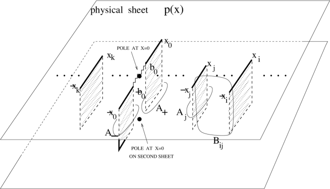
Figure 2: Hyperelliptic Riemann surface $\Sigma$, defined by equation (3.3); zig-zag line represents the condensate cut. There is a double pole of differential $dG$ at the image of the origin $x=0$ on the second sheet, while the differential $dp$ has double poles at $x=0$ on both sheets. The sheet where $dG$ has no singularities is called physical.

Equation (3.4) imposes an integrality condition on the ${\bf B}$-periods of $dp$,

$$\begin{array}[]{c}\oint_{B_{i}}dp=2\pi(n_{i}-n_{K})\qquad i=1,\ldots,K-1,\end{array}$$ (3.5)

for the canonical choice of the ${\bf B}$-cycles on the hyperelliptic surface, $B_{i}\equiv B_{iK}$ (see fig. 2). In the absence of condensates the single-valuedness of $p(x)$ on a physical sheet requires in addition that ${\bf A}$-periods are zero,

$$\begin{array}[]{c}\oint_{A_{i}}dp=0\qquad i=1,\ldots,K-1,\end{array}$$ (3.6)

for the canonical $A_{i}$ cycles on the hyperelliptic surface (fig. 2).

Figure 3: The contour of integration in (3.7). The marked points on two sheets correspond to infinities $\infty_{+}$ and $\infty_{-}$ where $x=\infty$.

We need an extra condition to satisfy all $K$ equations in (3.2). To find it, one can rewrite the $K$-th equation in (3.2) as

$$\begin{array}[]{c}p(\infty_{+})-p(\infty_{-})=\int_{\infty_{-}}^{\infty_{+}}dp=2\pi n_{K},\end{array}$$ (3.7)

where by $\infty_{+}$ and $\infty_{-}$ we denoted two points with $x=\infty$ on the first and second sheets of $\Sigma$ respectively. The contour of integration comes from the infinity on the physical sheet, passes through the $K$-th cut ${\bf C}_{K}$ onto the second sheet, and then goes to the infinity on this sheet (fig. 3). The points $\infty_{+}$ and $\infty_{-}$ are marked by the fact that the differential $xdp$, which determines the number of Bethe roots, has first order poles there (with residues of opposite sign), though $dp$ itself is non-singular. Note that since the choice of the cut $K$ is arbitrary we could choose the set of equations similar to (3.7) on all $K$ cuts to replace the equations (3.5).

Since $dp$ has second-order poles at $x=0$ on both sheets of the Riemann surface, it is of the general form

$$\begin{array}[]{c}dp={dx\over y}\sum_{k=-1}^{K-1}a_{k}x^{k-1}.\end{array}$$ (3.8)

The pole at $x=0$ on the physical sheet must be cancelled in $G(x)$, which requires $dp={dx\over 2x^{2}}+O(1)$ and fixes the first two coefficients to be

$$\begin{array}[]{c}a_{-1}=\frac{\sqrt{r_{2K}}}{2},~{}~{}~{}~{}~{}a_{0}={r_{2K-1}\over 4\sqrt{r_{2K}}}.\end{array}$$ (3.9)

The system of equations (3.6) uniquely determines the rest of the $K-1$ coefficients $a_{k}$ and thus completely defines the differential (3.8) on a given Riemann surface (3.3). The rest of the conditions are conditions on the moduli of the Riemann surface itself.

All together the curve (3.3) is parameterized by $2K$ end-points of the cuts ${\bf C}_{i}$. The integrality of ${\bf B}$-periods expressed by the eqs.(3.5) and the extra condition (3.7) constitute a system of $K$ equations on the coefficients of (3.3) and thus reduce the total number of free parameters to $K$. These free parameters exactly correspond to the filling fractions of the Bethe roots on the $K$ cuts ${\bf C}_{j}$,

$$\begin{array}[]{c}S_{j}={1\over 2\pi i}\oint_{A_{j}}p(x)dx=\int_{{\bf C}_{j}}\rho(x)dx,\ \ \ \ j=1,\dots,K-1\\ S_{K}={1\over 2\pi i}\oint_{{\bf C}_{K}}p(x)dx=\int_{{\bf C}_{K}}\rho(x)dx=\alpha-\sum_{j=1}^{K-1}S_{j}\end{array}$$ (3.10)

The residue at infinity determines the total number of Bethe roots :

$$\begin{array}[]{c}\frac{1}{2}-\alpha=-{1\over 2\pi i}{\rm res}_{\infty}xdp\end{array}$$ (3.11)

The normalization condition immediately allows us to set $a_{K-1}={\textstyle{1\over 2}}-\alpha$. The total momentum (2.17) can be rewritten in terms of the filling fractions $S_{j}$ in (3.10) as

$$\begin{array}[]{c}P=-{1\over 2\pi i}{\rm res}_{x=0}\ {p(x)dx\over x}=2\pi\sum_{j=1}^{K}n_{j}S_{j}=2\pi m.\end{array}$$ (3.12)

The anomalous dimension (2.18) can be now expressed directly through the parameters of the hyperelliptic curve (3.3) and of the quasimomentum (3.8) or resolvent $G(x)$. From the expansion of $p(x)$ at $x=0$,

$$p(x)=-{1\over 2x}-2\pi m-{8\pi^{2}L\gamma\over\lambda}\,x+O(x^{2}),$$

we have

$$\begin{array}[]{c}\gamma={\lambda\over 8\pi^{2}L}\left({r_{2K-2}\over 4r_{2K}}-\frac{r^{2}_{2K-1}}{16r^{2}_{2K}}-{a_{1}\over\sqrt{r_{2K}}}\right)\end{array}$$ (3.13)

which is a general solution for the one-loop anomalous dimension of “long” operators (1.1). It is expressed explicitly through the coefficients of the equation (3.3) which defines the complex curve, and by $a_{1}$ which is determined through the solution of the linear system (3.6), and is a transcendental function of the coefficients of (3.3). The coefficients of (3.3) are themselves defined implicitly as functions of the mode numbers $n_{j}$, the total momentum $P=2\pi m$, and the filling fractions $S_{j}$.

Figure 4: When an A-cycle crosses the condensate, $\oint_{A_{i}}dp=\,{\rm Disc}\,p=2\pi m_{i}$.

Very little changes if we allow for condensates. The differential of the quasi-momentum is still an Abelian differential of the second kind, the equations (3.2) are still solved by imposing integrality of ${\bf B}$-periods on $dp$ and an extra condition (3.7). The only difference is in the ${\bf A}$-periods. If an A-cycle $A_{i}$ crosses the condensate cut, $p$ jumps by $2\pi m_{i}$, where $m_{i}$ is an integer. Hence, ${\bf A}$-periods are no longer zero but are also integral (fig. 4). We thus get a very symmetric set of conditions on the periods of $dp$,

$$\begin{array}[]{c}\oint_{B_{i}}dp=2\pi(n_{i}-n_{K}),\\ \oint_{A_{i}}dp=2\pi m_{i}\end{array}$$ (3.14)

The counting of parameters does not change. There are $2K-1$ equations (A and B cycle conditions and (3.7)) on the total of $3K-1$ parameters ($2K$ moduli of the hyperelliptic curve $\Sigma$ and $K-1$ free coefficients in the definition of $dp$. eq. (3.8)). The $K$ parameter freedom reflects the possibility to redistribute Bethe roots over the $K$ cuts with arbitrary filling fractions (3.10). The overall normalization (3.11) fixes the total number of the roots and leaves $K-1$ independent parameters.

The approach of this section allows one to calculate the resolvent and consequently all the conserved charges for a given Bethe state in the scaling limit. It may seem that Bethe states are in one-to-one correspondence with the sets of $K$ filling fractions and $2K-1$ integers $\{n_{i},m_{i}\}$, but this is not quite true. Not all sets of parameters are allowed, since some of them give rise to complex curves that do not satisfy the reality condition, which therefore is a constraint on allowed values of integers $n_{i}$ and $m_{i}$. Also, some different sets of $n$’s and $m$’s may correspond to the same Bethe state. Suppose that we solved for the resolvent and found all its branch points ${\rm x}_{j}$ as functions of the parameters. There are still many ways to connect these branch points by cuts ${\bf C}_{l}$. In principle, the cuts should be defined in such a way that the density $\rho(x)dx$ for $\rho(x)=\,{\rm Disc}\,G(x)={1\over 2\pi i}\left(G(x+i0)-G(x-i0)\right)$ is real and positive definite on the cuts. Near each branch point $dx\,\rho(x)\sim dx\,(x-{\rm x}_{j})^{1/2}$. There are three lines on which $dx\,(x-{\rm x}_{j})^{1/2}$ is real and positive, and therefore three cuts consistent with positivity can meet at each of the branch points. This leads to a discrete ambiguity in cutting the complex plane. This argument is standard in the discussion of multi-cut solutions of matrix models (see, e.g. [66, 68]). Any rearrangement of cuts or permutation of the branch points induces a linear transformation of the ${\bf A}$- and ${\bf B}$- cycles and therefore, according to (3.14), of the integers $n_{i}$ and $m_{i}$. The branch of the square root on the physical sheet may, however, change sign at infinity under such rearrangement. The change in sign of the residue of $xdp$ at infinity, according to (3.11), is equivalent to interchanging $\alpha$ with $1-\alpha$. If $\alpha>{\textstyle{1\over 2}}$ from the outset, by rearranging cuts we can always get a new $\alpha$ in the physical domain $0<\alpha<{\textstyle{1\over 2}}$. Therefore, an analytic continuation of a solution of the Bethe equations beyond $\alpha={\textstyle{1\over 2}}$ indeed corresponds to a physical Bethe state with $\alpha<{\textstyle{1\over 2}}$. The energy and all local charges are modular invariant and do not change under the rearrangements of cuts. Since local charges completely characterize a Bethe state, we can relax even the reality condition for the density, and connect the branch points by cuts in an arbitrary way. Then all $Sp(K-1,{\vbox{\hbox{\numbers\hbox to0.0pt{\hbox to0.0pt{Z\hss}\kern 0.8pt\vrule height=8.0pt,width=0.5pt,depth=-5.9pt\hss}\kern 2.2pt\hbox to0.0pt{Z\hss}\kern 6.0pt\vrule height=2.0pt,width=0.5pt,depth=0.1pt\kern 1.0pt}}})$ transformations of cycles are allowed. In particular, it is always possible to set all ${\bf A}$-periods of $dp$ to zero by an appropriate $Sp(K-1,{\vbox{\hbox{\numbers\hbox to0.0pt{\hbox to0.0pt{Z\hss}\kern 0.8pt\vrule height=8.0pt,width=0.5pt,depth=-5.9pt\hss}\kern 2.2pt\hbox to0.0pt{Z\hss}\kern 6.0pt\vrule height=2.0pt,width=0.5pt,depth=0.1pt\kern 1.0pt}}})$ transformation. In other words, it is always possible to get rid of the condensates. This remark will be very important in the next section, when we will compare general solutions of the Bethe ansatz with classical solutions of the sigma-model. This discussion may seem somewhat abstract, but we hope to clarify it with explicit calculations for two-cut solutions in section 5.

A similar ambiguity affects the total momentum (3.12)

$$\begin{array}[]{c}P=-G(0)=\int_{0}^{\infty_{+}}dG.\end{array}$$ (3.15)

The contour of integration connects zero and infinity on the physical sheet and is otherwise arbitrary. Adding an A-cycle $A_{i}$ to it shifts the momentum by $2\pi m_{i}$, but the momentum is defined only up to an integer multiple of $2\pi$, and only ${\,\rm e}\,^{iP}$ makes sense. The case when the condensate passes through zero [32] requires special care, because in that case the integral in (3.15) is ambiguous and should be defined symmetrically such that the corresponding $A$-cycle contributes half of the period into the momentum. With this prescription the condensate of density $m$ (Bethe roots stretched along the imaginary axis with the spacing $im$) has the momentum $m\pi$. Indeed, careful inspection of the general formula (2.8) shows that an evenly spaced condensate has ${\,\rm e}\,^{iP}=1$, while an oddly spaced distribution of roots gives ${\,\rm e}\,^{iP}=-1$.

The Bethe equations (2.7) have an obvious symmetry, $u_{j}\to-u_{j}$, in which case the numerator replaces the denominator and vice versa. Therefore, sometimes it is rather natural to consider a class of solutions, when magnetic numbers satisfy $n(-u_{j})=-n(u_{j})$, Then the curve (3.3) has a symmetry $x\to-x$, i.e.

$$\begin{array}[]{c}y^{2}=\prod_{j=1}^{K}(x^{2}-{\rm x}_{j}^{2})\end{array}$$ (3.16)

The counting here is slightly different. We start from $K$ independent parameters (instead of $2K$), impose $K/2$ constraints (3.7), since $K$ should be even in this case, and the rest of parameters are eaten by the residue of the differential $xdp$ (3.11) and half of the independent “fractions” (3.10). A particular example of a symmetric solution will be considered in section 5.4.

3.2 Two-loop corrections

By this approach we can find also the two-loop corrections to our general one-loop solution, thus diagonalizing the operator (1.2) in the classical limit, using the two-loop perturbative integrability hypothesis proposed in [38] and confirmed in [39, 40]. A way to take higher loop corrections into account is to consider the Inozemtsev generalization of the spin-chain in the hyperbolic limit [48], as was recently proposed by Serban and Staudacher [42].

The Inozemtsev chain has long range interactions between the sites, reflecting the fact that $g$-loop corrections to the dilatation operator involve spin-exchange separated by up to $g$ sites. The hyperbolic limit has one free parameter that describes the fall-off of the interaction and Serban and Staudacher [42] mapped this parameter to $\lambda/L^{2}$. They then showed that not only did the Inozemtsev chain reproduce the two and three-loop dilatation operators in [38, 39, 40], but it also matches the two-loop predictions for the string solitons in [20, 22]. However, the three-loop predictions in [42] differ with those in [20, 22], and furthermore, there is an explicit violation of BMN scaling starting at four loops [42]. Despite the fact that the equivalence of the full perturbative SYM to the Inozemtsev chain is still only a hypothesis, the two-loop corrections are robust, and so we can use it to study the anomalous dimensions of general operators at the two-loop level and compare these with predictions of quasiclassical string theory.

The two-loop corrected Bethe equations look as follows [42]

$$\begin{array}[]{c}e^{ip_{j}L}=\prod_{k=1(k\neq j)}^{J}{u_{j}-u_{k}+i\over u_{j}-u_{k}-i},\par\par\end{array}$$ (3.17)

where the momentum $p_{j}=p_{j}(u_{j})$ is defined by solving the equation

$$\begin{array}[]{c}u=u_{0}(p)+{\lambda\over 8\pi^{2}}\sin p+O(\lambda^{2})\end{array}$$ (3.18)

with the function $u_{0}(p)$ given by

$$\begin{array}[]{c}e^{ip}={u_{0}+i/2\over u_{0}-i/2},\end{array}$$ (3.19)

Up to two-loop order, eq. (3.17) can be rewritten as

$$\begin{array}[]{c}\left({u_{j}+i/2-{\lambda\over 8\pi^{2}}{u_{j}\over u_{j}^{2}+1/4}\over u_{j}-i/2-{\lambda\over 8\pi^{2}}{u_{j}\over u_{j}^{2}+1/4}}\right)^{L}=\prod_{k=1(k\neq j)}^{J}{u_{j}-u_{k}+i\over u_{j}-u_{k}-i},\end{array}$$ (3.20)

This means that in the classical limit $u=xL$, $L\to\infty$, eq. (2.15) is corrected as follows

$$\begin{array}[]{c}{1\over x}+{\lambda\over 8\pi^{2}L^{2}}{1\over x^{3}}+2\pi n_{l}=2{-\!\!\!\!\!\!\int}_{{\bf C}}{d\xi\,\rho(\xi)\over x-\xi},\ \ \ x\in{\bf C}_{l}\end{array}$$ (3.21)

with the same normalization of the density (2.14) as in the one-loop case. Note however, that being perturbative from the gauge theory side, the second term in the l.h.s. of (3.21) is “singular” perturbation of the integrable system, since it adds a singularity of higher degree. For example, analogous perturbation in the algebraic matrix model case [66, 67] would change the genus of the curve. Here, it will causes some problems, when comparing with the string theory side.

The two-loop generalization of the total momentum quantization condition (2.8) can be rewritten as

$$\begin{array}[]{c}\prod_{j=1}^{J}\left({u_{j}+i/2-{\lambda\over 8\pi^{2}}{u_{j}\over u_{j}^{2}+1/4}\over u_{j}-i/2-{\lambda\over 8\pi^{2}}{u_{j}\over u_{j}^{2}+1/4}}\right)^{L}=1\end{array}$$ (3.22)

or, in the classical limit,

$$\begin{array}[]{c}2\pi m=\int dx\,\rho(x)\left({1\over x}+{\lambda\over 8\pi^{2}L^{2}}{1\over x^{3}}\right)+O(\lambda^{2})=-\int{dx\over 2\pi i}\,G(x)\left({1\over x}+{\lambda\over 8\pi^{2}L^{2}}{1\over x^{3}}\right)+O(\lambda^{2})\end{array}$$ (3.23)

The anomalus dimension is corrected as follows [42]:

$$\begin{array}[]{c}\gamma=\sum_{j=1}^{J}\left[{\lambda\over 2\pi^{2}}\sin^{2}{p(u_{j})\over 2}-{\lambda^{2}\over 8\pi^{4}}\sin^{4}{p(u_{j})\over 2}\right]+O(\lambda^{3})=\\ =\sum_{j=1}^{J}\left[{\lambda\over 8\pi^{2}}{1\over u_{j}^{2}+1/4}+{3\lambda^{2}\over 128\pi^{4}}{1\over(u_{j}^{2}+1/4)^{2}}-{\lambda^{2}\over 128\pi^{4}}{1\over(u_{j}^{2}+1/4)^{3}}\right]+O(\lambda^{3})\end{array}$$ (3.24)

In the classical limit $L\to\infty$ this two-loop formula corrects eq.(2.18) in the following way

$$\begin{array}[]{c}\gamma=L\int dx\,\rho(x)\left({\lambda\over 8\pi^{2}L^{2}}{1\over x^{2}}+{3\lambda^{2}\over 128\pi^{4}L^{4}}{1\over x^{4}}+O\left({\lambda^{2}\over L^{6}}\right)+O(\lambda^{3})\right)=\\ =-\oint{dx\over 2\pi i}\,G(x)\left({\lambda\over 8\pi^{2}L}{1\over x^{2}}+{3\lambda^{2}\over 128\pi^{4}L^{3}}{1\over x^{4}}+O\left({\lambda^{2}\over L^{5}}\right)+O\left(\lambda^{3}\right)\right)\end{array}$$ (3.25)

We kept here only the terms relevant in the BMN limit of fixed $T={\lambda\over 16\pi^{2}L^{2}}$.

We can now solve eq. (3.21) in the same way as (2.15). We introduce

$$\begin{array}[]{c}p(x)=G(x)-{1\over 2x}-{T\over x^{3}}\end{array}$$ (3.26)

and find for the differential $dp$ on the Riemann surface (3.3) the following modification to (3.8)

$$\begin{array}[]{c}dp={dx\over y}\sum_{k=-3}^{K-1}a_{k}x^{k-1}.\end{array}$$ (3.27)

with the condition that $dp={1\over 2x^{2}}+{3T\over x^{4}}+O(1)$ for $x\to 0$. It is clear that this gives two extra conditions to fix the two extra coefficients $a_{-3}$ and $a_{-2}$.

Below we will compare these results with the two-loop correction following from the sigma-model results, where the term ${1\over x^{3}}$ will appear from the two-pole structure ${1\over 2}\left({1\over x-1}+{1\over x+1}\right)\simeq{1\over x}+{1\over x^{3}}+O\left({1\over x^{5}}\right)$ in the integral equation similar to (3.21). We will see that although the structures are very similar, the details are different. In contrast to one loop, where the equations are easily reproduced from those of the string sigma model, the two-loop equations of this section follow from the integrable equations of string theory only after a reparameterization of the spectral parameter. This basically reflects the fact that the choice of the spectral parameter in (3.18) and (3.21) is somewhat arbitrary. Nevertheless, they lead to the same results for the anomalous dimension up to the two-loop level. In section 5 we will present a wide class of examples where the agreement is explicitly checked.

4 Classical integrability

We now turn to integrability on the string side of the AdS/CFT duality. Classical integrability of the sigma-model in the $AdS_{5}\times S^{5}$ background [44, 43] means, among other things, that the classical equations of motion of a string in $AdS_{5}\times S^{5}$ can be solved by algebro-geometric methods [69, 70, 71, 72] or, for certain particular cases, by the inverse scattering transformation [73]. In this section, we will examine finite-gap periodic solutions of the sigma-model and establish direct links between them and the Bethe ansatz. A pedagogic introduction into finite-gap integration methods can be found, for example, in the monographs [71, 72], and the comparison of quantum inverse scattering with classical integrability, applied mostly to the nonlinear Schrödinger and KdV equations, can be found in [36, 37].

As in the discussion of the SYM operators we will focus on an $SU(2)$ reduction of the full sigma-model to the subsector of string moving on $S^{3}\times{R}_{t}$. Many explicit solutions are known in this case [26]. The string action in the conformal gauge is

$$\begin{array}[]{c}S_{\sigma m}={\sqrt{\lambda}\over 4\pi}\int_{0}^{2\pi}d\sigma\,\int d\tau\,\left[\left(\partial_{a}X_{i}\right)^{2}-\left(\partial_{a}X_{0}\right)^{2}\right],\end{array}$$ (4.1)

where $X_{0}$ is the global AdS time and $X_{i}$, $i=1,\ldots,4$ are Cartesian coordinated on $S^{3}$ embedded in ${R}^{4}$:

$$\begin{array}[]{c}X_{i}X_{i}=1.\end{array}$$ (4.2)

All other world-sheet coordinates (one radial and three angular coordinates on $AdS_{5}$ and two extra angles on $S^{5}$) are set to constant values. Such an ansatz describes a string localized in the centre of AdS and moving in an $S^{3}$ subspace of $S^{5}$. The effective string tension is related to the ’t Hooft coupling according to AdS/CFT [7]. The equations of motion that follow from (4.1) should be supplemented with the Virasoro constraints:

$$\begin{array}[]{c}(\partial_{\pm}X_{i})^{2}=(\partial_{\pm}X_{0})^{2}=\kappa^{2},\end{array}$$ (4.3)

where $\sigma_{\pm}={\textstyle{1\over 2}}(\tau\pm\sigma)$, $\partial_{\pm}=\partial_{\tau}\pm\partial_{\sigma}$, and we always consider a gauge $X_{0}=\kappa\tau$.

It was shown in [35] that the equations of motion for the string whose centre of mass moves along a big circle of $S^{3}$ with a large angular momentum have a well-defined weak-coupling limit ($\lambda/L^{2})\ll 1$, where now $\sqrt{\lambda}$ is the effective string tension and $L$ is the angular momentum, and reduce in this limit to

$$\begin{array}[]{c}\sin\theta\partial_{\tau}\theta+\partial_{\sigma}(\sin^{2}\theta\partial_{\sigma}\varphi)=0\\ \partial^{2}_{\sigma}\theta-\sin\theta\partial_{\tau}\varphi-\sin\theta\cos\theta(\partial_{\sigma}\varphi)^{2}=0,\end{array}$$ (4.4)

where $\varphi$ and $\theta$, in addition to another angle that parameterizes the motion of the centre of mass, are coordinates on $S^{3}$. This limit can be regarded as an approximation of an almost light-like string motion [74] In terms of a unit vector, ${\bf S}=(\sin\theta\,\cos\varphi,\sin\theta\,\sin\varphi,\cos\theta)$ the equations (4.4) take the form

$$\begin{array}[]{c}{\bf S}_{\tau}={\bf S}\times{\bf S}_{\sigma\sigma}.\end{array}$$ (4.5)

This is the equation of the classical Heisenberg model. It can be formally obtained from operator equations of motion in the spin chain by replacing quantum spins ${{\mathchoice{\hbox{$\displaystyle\sigma$}}{\hbox{$\textstyle\sigma$}}{\hbox{$\scriptstyle\sigma$}}{\hbox{$\scriptscriptstyle\sigma$}}}}_{l}$ with ${\bf C}$-number unit vectors ${\bf S}$ and simultaneously taking the continuum limit: ${{\mathchoice{\hbox{$\displaystyle\sigma$}}{\hbox{$\textstyle\sigma$}}{\hbox{$\scriptstyle\sigma$}}{\hbox{$\scriptscriptstyle\sigma$}}}}_{l}(\tau)\rightarrow{\bf S}(2\pi l/L,\tau)={\bf S}(\sigma,\tau)$. In [35] Kruczenski presented a path-integral derivation of this fact, and identified this classical approximation with the limit of the large size of the chain in which only slowly varying spin configurations are kept.

The classical Heisenberg equation is completely integrable [75, 76, 77, 73] and is a particular case of a more general Landau-Lifshitz equation

$$\begin{array}[]{c}{\bf S}_{t}={\bf S}\times{\bf S}_{\sigma\sigma}+{\bf S}\times J{\bf S}\end{array}$$ (4.6)

where $J$ is an anisotropy matrix which is proportional to the unit matrix in our case, so that second term in the r.h.s. vanishes and (4.6) turns into (4.5) . We examine the classical Heisenberg equations in the next section and establish an equivalence between their periodic solutions and the general scaling solution of the Bethe ansatz which was obtained in section 3.

4.1 Finite-gap solutions of the Heisenberg magnet

In order to relate integrable structures of the classical and quantum Heisenberg models, let us perform a continuous limit directly to the transfer matrix (2.2). If we replace ${{\mathchoice{\hbox{$\displaystyle\sigma$}}{\hbox{$\textstyle\sigma$}}{\hbox{$\scriptstyle\sigma$}}{\hbox{$\scriptscriptstyle\sigma$}}}}_{l}$ in (2.2) by ${\bf S}(2\pi l/L)$ and also rescale the spectral parameter $u=Lx$, then the transfer matrix becomes

$$\frac{T(Lx)}{(Lx)^{L}}\rightarrow{\rm Tr}\,\prod_{l=L}^{1}\left(1+\frac{i}{2xL}\,{\bf S}(2\pi l/L)\otimes{{{\mathchoice{\hbox{$\displaystyle\sigma$}}{\hbox{$\textstyle\sigma$}}{\hbox{$\scriptstyle\sigma$}}{\hbox{$\scriptscriptstyle\sigma$}}}}}\right).$$

This expression has a well-defined continuum limit, as an anti-path-ordered exponential

$$\begin{array}[]{c}\prod_{l=L}^{1}\left(1+\frac{i}{2xL}\,{\bf S}(2\pi l/L)\otimes{{{\mathchoice{\hbox{$\displaystyle\sigma$}}{\hbox{$\textstyle\sigma$}}{\hbox{$\scriptstyle\sigma$}}{\hbox{$\scriptscriptstyle\sigma$}}}}}\right)\ \mathrel{\mathop{\rightarrow}\limits_{L\to\infty}}\Omega(x)=\bar{P}\exp\left(\frac{i}{2x}\oint\frac{d\sigma}{2\pi}\,{\bf S}(\sigma)\cdot{{{\mathchoice{\hbox{$\displaystyle\sigma$}}{\hbox{$\textstyle\sigma$}}{\hbox{$\scriptstyle\sigma$}}{\hbox{$\scriptscriptstyle\sigma$}}}}}\right)\end{array}$$ (4.7)

which is just the monodromy matrix of the classical Heisenberg model, and we can introduce the classical quasimomentum $p(x)$ by

$$\begin{array}[]{c}\,{\rm Tr}\,\Omega(x)\equiv\lim_{L\rightarrow\infty}\frac{T(Lx)}{(Lx)^{L}}=2\cos p(x)\end{array}$$ (4.8)

The classical equations of the Heisenberg magnet are equivalent to the consistency condition $[L,M]=0$ of an auxiliary linear problem

$$\begin{array}[]{c}L\Psi=\left(\partial_{\sigma}-\frac{iU}{4\pi x}\right)\Psi(x;\tau,\sigma)=0\\ M\Psi=\left(\partial_{\tau}-\frac{iU}{4\pi^{2}x^{2}}+\frac{iV}{4\pi x}\right)\Psi(x;\tau,\sigma)=0\end{array}$$ (4.9)

where the Lax matrices are

$$\begin{array}[]{c}U={{{\mathchoice{\hbox{$\displaystyle\sigma$}}{\hbox{$\textstyle\sigma$}}{\hbox{$\scriptstyle\sigma$}}{\hbox{$\scriptscriptstyle\sigma$}}}}}\cdot{\bf S}\\ V={{{\mathchoice{\hbox{$\displaystyle\sigma$}}{\hbox{$\textstyle\sigma$}}{\hbox{$\scriptstyle\sigma$}}{\hbox{$\scriptscriptstyle\sigma$}}}}}\cdot\left({\bf S}_{\sigma}\times{\bf S}\right)\end{array}$$ (4.10)

The monodromy matrix is a parallel transporter of the flat connection $(L,M)$ around the circle: $\Omega(x)=\Psi(x;\tau_{0},1)$, where $\Psi(x;\tau,\sigma)$ is the solution of (4.9) with the initial condition $\Psi(x;\tau_{0},0)=1$. Since the connection is flat the trace of the monodromy matrix does not depend on $\tau_{0}$ and therefore generates an infinite set of integrals of motion. The classical monodromy matrix is unimodular and unitary when the spectral paramater is real. Its eigenvalues ${\,\rm e}\,^{\pm ip(x)}$ then determine the quasi-momentum $p(x)$, and the Taylor expansion of the quasi-momentum generates an infinite set of conserved charges, which are local functionals of ${\bf S}(\tau,\sigma)$ [73].

From section 2 we know that taking the scaling limit of the quantum transfer matrix in (2.5) leads to

$$\begin{array}[]{c}2\cos p(x)\equiv\frac{T(Lx)}{(Lx)^{L}}=2\cos\left(G(x)-\frac{1}{2x}\right),\end{array}$$ (4.11)

with the resolvent defined in (2.12). There is a $1/(2x)$ correction term in (4.11) because, unlike in (2.3), we did not shift the spectral parameter by $i/2$. We conclude that the resolvent constructed from the density of Bethe roots and the quasi-momentum of the classical problem are related exactly as in (3.1). The local conserved charges in the spin chain and in the classical Heisenberg model are thus equivalent. This observation elucidates the meaning of the transformations used in [46] to relate higher conserved charges in the sigma-model to the conserved charges of the spin chain. The approach of [46] is based on Bäcklund charges, which differ from charges defined by the expansion of quasi-momentum. One has to do a linear transformation on an infinite set of charges to account for this difference.

The transformation of the quantum spin operators into the c-number unit vectors is hard to motivate rigorously in the present context. There is a more direct way to compare the Bethe ansatz of the quantum spin chain and the auxiliary linear problem of the classical model, which allows one to derive (3.1) directly, by inspecting the analytic structure of the quasi-momentum. Moreover, this method can be generalized to the sigma-model, where the quantum counterpart (all-loop Bethe anzatz) is not yet known.

It is always possible to reconstruct the solution of the Heisenberg equation from the solution of the auxiliary linear problem. Indeed, it follows from (4.9), and (4.10) that

$$\begin{array}[]{c}{\bf S}=-2\pi ix\,{\rm Tr}\,\left({{\mathchoice{\hbox{$\displaystyle\sigma$}}{\hbox{$\textstyle\sigma$}}{\hbox{$\scriptstyle\sigma$}}{\hbox{$\scriptscriptstyle\sigma$}}}}\,\Psi_{\sigma}\Psi^{-1}\right).\end{array}$$ (4.12)

A slightly less trivial statement is that $\Psi(x;\tau,\sigma)$ is essentially determined by the analytic properties of the quasi-momentum $p(x)$. Let us now establish these properties by inspecting the auxiliary problem (4.9).

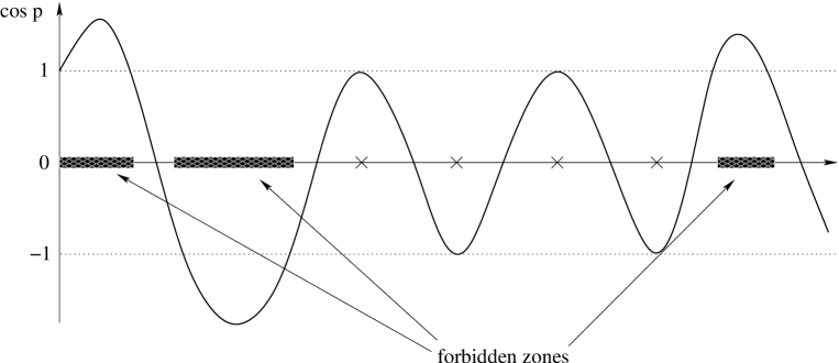
Figure 5: The trace of the monodromy matrix as a function of the spectral parameter along the curve on which $\cos p(x)$ is real. The crosses correspond to degenerate periodic solutions, which represent forbidden zones shrunk to points.

The linear problem (4.9) has a form of a one-dimensional Dirac equation

$$\begin{array}[]{c}\left(\partial_{\sigma}-\frac{i{\bf S}\cdot{{{\mathchoice{\hbox{$\displaystyle\sigma$}}{\hbox{$\textstyle\sigma$}}{\hbox{$\scriptstyle\sigma$}}{\hbox{$\scriptscriptstyle\sigma$}}}}}}{4\pi x}\right)\psi=0,\end{array}$$ (4.13)

were $\psi$ is a two-component spinor. Two linearly independent solutions of this equation can be chosen quasi-periodic. Indeed, if the initial conditions are eigenvalues of the monodromy matrix

$$\begin{array}[]{c}\Omega(x)\psi_{\pm}(x;0)={\,\rm e}\,^{\pm ip(x)}\psi_{\pm}(x;0),\end{array}$$ (4.14)

the solution $\psi_{\pm}(x;\sigma)=\Psi(x;\sigma)\psi_{\pm}(x;0)$ will again satisfy $\psi_{\pm}(x;\sigma+2\pi)={\,\rm e}\,^{\pm ip(x)}\psi_{\pm}(x;\sigma)$ because $\Psi(x;\sigma+2\pi)=\Psi(x;\sigma)\Omega(x)$.

However, the quasi-momentum is not neccesarily real, being in general, a complex-valued function of the spectral parameter. The condition that its imaginary part vanish is a single equation on two variables (the real and imaginary parts of the complex spectral parameter $x$). Therefore, the quasi-momentum is real on a set of disjoint one-dimensional supports (some segments in the complex plane of $x$). These segments correspond to allowed zones of the spectral problem (4.13). In a more familiar setup of the Schrödinger equation with a periodic potential, the allowed energy zones lie on the real axis, but the operator (4.13) is not Hermitean. The allowed zones are singled out by the condition that ${\rm Im}\,\left({\rm Tr}\,\Omega\right)=0$ and $|{\rm Tr}\,\Omega|<2$. One can also define forbidden zones as loci where ${\rm Im}\,\left({\rm Tr}\,\Omega\right)=0$ and $|{\rm Tr}\,\Omega|>2$, see fig. 5. In general the number of allowed and forbidden zones is infinite. We will only discuss finite-gap, or algebro-geometric solutions for which this number is finite. They are governed by the geometry of a complex curve of finite genus (3.3) and directly correspond to solutions of the Bethe equations with a finite number of cuts. In other words, it is more convenient to work with the smooth non-degenerate curve (3.3) than with the curve, defined by the Baxter equation on quasimomentum $\det(\Omega-e^{ip})=0$ or

$$\begin{array}[]{c}{\,\rm e}\,^{ip}+{\,\rm e}\,^{-ip}=\,{\rm Tr}\,\Omega(x)\end{array}$$ (4.15)

which is generally a degenerate curve of an infinite genus.

At zone boundaries the monodromy matrix degenerates into the Jordan cell and has only one eigenvector with an eigenvalue $1$ or $-1$. The quasi-momentum becomes an integer multiple of $\pi$ and the two independent solutions of (4.13) become degenerate. This degenerate solution of (4.13) is either periodic or anti-periodic. Accidental periodic and anti-periodic solutions may appear inside some of the allowed zones (see fig. 5). They are always present for finite-gap potentials, and this is related to the fact that $p(x)$ is not an algebraic function on (3.3). The linear problem (4.13) still has two independent (anti)-periodic solutions at these special points. Hence, $\Omega$ is either $+{\bf 1}$ or $-{\bf 1}$, and these points do not correspond to zone boundaries. They rather represent forbidden zones shrunk to a point and of course are not generic, as much as finite-gap solutions are not generic in the space of all solutions to the Heisenberg magnet equations.

The zone boundaries are singular points for $\psi_{\pm}(x;\sigma)$ as functions of $x$, because $\psi_{\pm}$ collapses into one degenerate solution there. It is thus natural to regard $\psi_{+}$ and $\psi_{-}$ as two branches of a single analytic function $\psi$ on a double cover of the complex $x$ plane. The zone boundaries are branch points at which the two branches collide. Apart from an essential singularity at $x=0$, $\psi$ is a holomorphic function on a hyperelliptic curve, two sheets of which are glued together along the forbidden zones. This is how the Riemann surface $\Sigma$, defined by (3.3), arises in the auxiliary problem of the classical Heisenberg model. The two eigenvalues of the monodromy matrix, ${\,\rm e}\,^{\pm ip(x)}$ are also branches of a single meromorphic function on $\Sigma$. In fact, the trace of the monodromy matrix is an entire function of $x$. There is no reason for it to be singular anywhere, except at $x=0$ where the potential in (4.13) has a singularity. But solving (4.15) for $p$ we will encounter square root singularities when the discriminant of the quadratic equation (4.15), with respect to ${\,\rm e}\,^{ip}$, becomes zero. This is another way to see why the quasi-momentum has branch points.

The matrix solution of (4.9), $\Psi(x;\tau,\sigma)$, is a meromorphic function on $\Sigma$ as well. This latter function has the following asymptotic behavior:

$$\begin{array}[]{c}\Psi(x;\tau,\sigma)\ \mathrel{\mathop{\sim}\limits_{x\to 0}}\ \exp\left[i\sigma_{3}\left({\sigma\over 4\pi x}+{\tau\over 4\pi^{2}x^{2}}\right)\right]\cdot\Phi(x;\tau,\sigma)\cdot C\end{array}$$ (4.16)

where $C$ is just a constant matrix (independent of $x$, $\tau$ and $\sigma$), and

$$\begin{array}[]{c}\Phi(x;\tau,\sigma)=\phi_{0}(\tau,\sigma)+\sum_{k>0}\phi_{k}(\tau,\sigma)x^{k}\end{array}$$ (4.17)

is regular at $x=0$. An analytic matrix function (4.16) on the hyperelliptic Riemann surface (3.3) with such asymptotics and $g+1$ extra poles, which can be chosen independent of $\tau$ and $\sigma$, is unique, they can be expressed in terms of the Riemann theta-functions [78] by the standard technique of finite-gap integration.

Let us return to the analytic properties of the quasi-momentum. Consider the values of the quasi-momentum $p(x+i0)$ and $p(x-i0)$ on the two sides of a forbidden zone. Shifting infinitesimally the point $x-i0$ towards the forbidden zone, one can pass it through the cut onto the second sheet. Thus $p(x+i0)$ and $p(x-i0)$ can be regarded as two branches of a double-valued function $p(x)$ at the same point on the complex $x$-plane. One can think of ${\,\rm e}\,^{ip(x+i0)}$ and ${\,\rm e}\,^{ip(x-i0)}$ as two independent solutions of the chracteristic (4.15) equation for the monodromy matrix. Since $\Omega(x+i0)$ is unimodular, ${\,\rm e}\,^{ip(x+i0)}{\,\rm e}\,^{ip(x-i0)}=1$, and the quasi-momentum must satsify

$$\begin{array}[]{c}p(x+i0)+p(x-i0)=2\pi n_{k},~{}~{}~{}~{}~{}x\in{\bf C}_{k}\end{array}$$ (4.18)

on each of the forbidden zones. This equation represents a Riemann-Hilbert problem equivalent to (3.2), if the quasi-momentum and the resolvent are related as in (3.1). The integer $n_{k}-n_{k-1}-1$ is the number of (anti)-periodic solutions within the $k$-th allowed zone, that is the number of times the equation ${\rm Tr}\,\Omega(x)=2$ is satisfied as $x$ moves along the allowed zone between the forbidden zones ${\bf C}_{k-1}$ and ${\bf C}_{k}$. Equivalently, $n_{k}-n_{k-1}-1$ is the number of oscillations $\cos p(x)$ makes between the end-points of the forbidden zones ${\bf C}_{k-1}$ and ${\bf C}_{k}$ (see fig. 5).

We see that, in the classical system, the integrality of ${\bf B}$-periods (3.5) essentially follows from the unimodularity of the transfer matrix. Since $p(x)$ is single-valued outside of the cuts, all ${\bf A}$-periods are zero. In other words, there are no condensate cuts. As we remarked in section 3, it is always possible to choose cuts in such a way that condensates “evaporate” and all ${\bf A}$-periods of $dp$ identially turn to zero. Such a choice of cuts is unique and corresponds precisely to cutting the $x$-plane along the forbidden zones. The condition that defines the forbidden zones, ${\rm Im}\,{\rm Tr}\,\Omega=0$ and $|{\rm Tr}\,\Omega|>2$, does not necessarily coincide with the condition that $-idx\,{\rm Disc}\,p$ be real and positive, which is appropriate for the Bethe ansatz. This is a crucial difference as compared to the quantum KdV equation, where Bethe roots condense on the forbidden zones of the classical problem [37].

A simple asymptotic analysis of the linear problem (4.13), (4.16) shows that the quasi-momentum behaves as $p(x)\sim\pm{1\over 2x}~{}~{}~{}{\rm at}~{}~{}~{}x\rightarrow 0$, this analysis amounts to solving equation

(4.13) in the WKB approximation. Hence, $G(x)=p(x)+{1\over 2x}$ is regular at zero on one of the sheets of the Riemann surface (3.3), and this singles out the physical sheet of $\Sigma$.

To complete a proof of equivalence between the Bethe equations and the classical auxiliary problem, we should also check that the reality of ${\bf S}(\tau,\sigma)$ reproduces the reality condition on the distribution of Bethe roots. The reality of ${\bf S}(t,\sigma)$ implies the following conjugation property of the monodromy matrix:

$$\begin{array}[]{c}\overline{\Psi}(x,t,\sigma)=\sigma_{2}\Psi(\bar{x};t,\sigma)\sigma_{2},~{}~{}~{}~{}~{}\overline{\Omega}(x)=\sigma_{2}\Omega(\bar{x})\sigma_{2},\end{array}$$ (4.19)

where the bar over matrices denotes complex conjugation of all matrix elements. If $\Omega(x)\psi={\,\rm e}\,^{ip(x)}\psi$, then $\overline{\Omega}(x)\bar{\psi}={\,\rm e}\,^{-i\bar{p}(x)}\bar{\psi}$, and $\Omega(\bar{x})\sigma_{2}\bar{\psi}={\,\rm e}\,^{-i\bar{p}(x)}\sigma_{2}\bar{\psi}$. Therefore, $\sigma_{2}\bar{\psi}$ is an eigenvector of $\Omega(\bar{x})$ with an eigenvalue ${\,\rm e}\,^{-i\bar{p}(x)}$, i.e. $p(\bar{x})=\bar{p}(x)$, which is indeed equivalent to the reality condition for the resolvent.

4.2 Finite-gap solutions of the chiral field

Since the three-sphere $S^{3}$ is the group manifold of $SU(2)$, the sigma-model (4.1)-(4.3) can be equivalently reformulated as an $SU(2)$ principal chiral field:

$$\begin{array}[]{c}g=\left(\begin{array}[]{cc}X_{1}+iX_{2}&X_{3}+iX_{4}\\ -X_{3}+iX_{4}&X_{1}-iX_{2}\end{array}\right)\equiv\left(\begin{array}[]{cc}Z_{1}&Z_{2}\\ -{\bar{Z}}_{2}&{\bar{Z}}_{1}\end{array}\right)\in SU(2),\\ g^{-1}dg=\left(\begin{array}[]{cc}{\bar{Z}}_{1}dZ_{1}+Z_{2}d{\bar{Z}}_{2}&{\bar{Z}}_{1}dZ_{2}-Z_{2}d{\bar{Z}}_{1}\\ {\bar{Z}}_{2}dZ_{1}-Z_{1}d{\bar{Z}}_{2}&{\bar{Z}}_{2}dZ_{2}+Z_{1}d{\bar{Z}}_{1}\end{array}\right)\in su(2).\end{array}$$ (4.20)

The action (4.1) takes the form

$$\begin{array}[]{c}S_{\sigma m}=-\frac{\sqrt{\lambda}}{4\pi}\int d\sigma d\tau\,\left[\frac{1}{2}\,{\rm Tr}j_{a}^{2}+(\partial_{a}X_{0})^{2}\right].\end{array}$$ (4.21)

where $j_{a}=g^{-1}\partial_{a}g={1\over 2i}j^{A}_{a}\sigma^{A}$ with $a=0,1=\tau,\sigma$, are the right currents. The equations of motion can be written in terms of their light-cone components as

$$\begin{array}[]{c}\partial_{+}j_{-}+\partial_{-}j_{+}=0,\ \ \ \ \ \partial_{+}\partial_{-}X_{0}=0,\\ \partial_{+}j_{-}-\partial_{-}j_{+}+[j_{+},j_{-}]=0.\end{array}$$ (4.22)

where the last equality follows from the expression for the currents in terms of the matrices $g$ in (4.20).

The sigma-model on $S^{3}$ possesses a global $SU_{L}(2)\times SU_{R}(2)$ symmetry which acts as $g(\tau,\sigma)$ by left and right multiplication by constant group matrices. This symmetry can be identified with a particular $SO(4)$ subgroup of the $SO(6)$ $R$-symmetry group of ${\cal N}=4$ SYM. The six scalar fields in the SYM transform under $SO(6)$ in the same way as the Cartesian coordinates on the five-sphere in the $AdS_{5}\times S^{5}$ geometry. The fields ${\mbox{\boldmath$\Phi$}}_{1}$ and ${\mbox{\boldmath$\Phi$}}_{2}$ have the same quantum numbers under $SU_{L}(2)\times SU_{R}(2)$ as the sigma-model target space coordinates $Z_{1}$ and $Z_{2}$ defined in (4.20), i.e. ${\mbox{\boldmath$\Phi$}}_{1}\sim Z_{1}$ and ${\mbox{\boldmath$\Phi$}}_{2}\sim Z_{2}$. Under the left shifts, generated by

$$\begin{array}[]{c}Q_{L}^{A}=\frac{\sqrt{\lambda}}{4\pi}\int d\sigma\,l^{A}_{0},\end{array}$$ (4.23)

where $l_{a}=gj_{a}g^{-1}=\partial_{a}g\,g^{-1}$, we have $g\rightarrow hg$, and $(Z_{1},-\bar{Z}_{2})$ and $(Z_{2},-\bar{Z}_{1})$ transform as doublets. The normalization of the generator is such that $Z_{1}$ and $Z_{2}$ have $Q_{L}^{3}=1$. This implies that for an operator ${\rm Tr}({\mbox{\boldmath$\Phi$}}_{1}^{L-J}{\mbox{\boldmath$\Phi$}}_{2}^{J}+\ldots)$:

$$\begin{array}[]{c}Q_{L}^{3}=L.\end{array}$$ (4.24)

Under the right shifts, generated by

$$\begin{array}[]{c}Q_{R}^{A}=\frac{\sqrt{\lambda}}{4\pi}\int d\sigma\,j^{A}_{0},\end{array}$$ (4.25)

$g\rightarrow gh$, and $(Z_{1},Z_{2})$ transforms as a doublet, so that $Z_{1}$ has $Q_{R}^{3}=1$ and $Z_{2}$ has $Q_{R}^{3}=-1$. Consequently,

$$\begin{array}[]{c}Q_{R}^{3}=L-2J.\end{array}$$ (4.26)

The scaling dimension of an operator is dual to the energy of the string solution,

$$\begin{array}[]{c}\Delta=\frac{\sqrt{\lambda}}{2\pi}\int_{0}^{2\pi}d\sigma\,\partial_{\tau}X_{0}=\sqrt{\lambda}\,\kappa,\end{array}$$ (4.27)

which is generated by the global time translations. Thus, the Virasoro constraints (4.3) become

$$\begin{array}[]{c}{1\over 2}{\rm Tr}j_{+}^{2}={1\over 2}{\rm Tr}j_{-}^{2}=-\kappa^{2}\,.\end{array}$$ (4.28)

These constraints describe a consistent reduction of the $SU(2)$ chiral field introduced in [79]. Upon the identification

$$\begin{array}[]{c}j_{+}=i\kappa\,{\bf S}_{+}\cdot{{{\mathchoice{\hbox{$\displaystyle\sigma$}}{\hbox{$\textstyle\sigma$}}{\hbox{$\scriptstyle\sigma$}}{\hbox{$\scriptscriptstyle\sigma$}}}}},~{}~{}~{}~{}~{}j_{-}=i\kappa\,{\bf S}_{-}\cdot{{{\mathchoice{\hbox{$\displaystyle\sigma$}}{\hbox{$\textstyle\sigma$}}{\hbox{$\scriptstyle\sigma$}}{\hbox{$\scriptscriptstyle\sigma$}}}}},\end{array}$$ (4.29)

the model reduces to a system of two interacting spins of unit length ${\bf S}_{+}$ and ${\bf S}_{-}$:

$$\begin{array}[]{c}\partial_{+}{\bf S}_{-}+2\kappa{\bf S}_{-}\times{\bf S}_{+}=0,\\ \partial_{-}{\bf S}_{+}-2\kappa{\bf S}_{-}\times{\bf S}_{+}=0.\end{array}$$ (4.30)

These equations automatically incorporate the Virasoro constraints. The model has an interesting quantum version [79, 80, 31], which is a spin system with two spins per site. We do not see an obvious way to relate the two-spin chain of [79] to the dilatation operator of ${\cal N}=4$ SYM theory (though the Heisenberg model can be obtained in a certain limit, see below), but do not exclude the possibility that such a relationship may exist.

The equations of motion for the principal chiral field can be written as a flatness condition [70]. Define a current $J(x)$ dependent on a spectral parameter $x$ as

$$\begin{array}[]{c}J_{\pm}(x)=\frac{j_{\pm}}{1\mp x}\,.\end{array}$$ (4.31)

Then the zero-curvature equation

$$\begin{array}[]{c}\partial_{+}J_{-}-\partial_{-}J_{+}+[J_{+},J_{-}]=0\end{array}$$ (4.32)

is equivalent to (4.22).

On the other hand, it is straightforward to show that (4.32) is equivalent to the consistency condition of the following linear problem

$$\begin{array}[]{c}{\cal L}\Psi=\left(\partial_{\sigma}+{1\over 2}\left({j_{+}\over 1-x}-{j_{-}\over 1+x}\right)\right)\Psi=\left[\partial_{\sigma}+\frac{i\kappa}{2}\left({{\bf S}_{+}\cdot{{{\mathchoice{\hbox{$\displaystyle\sigma$}}{\hbox{$\textstyle\sigma$}}{\hbox{$\scriptstyle\sigma$}}{\hbox{$\scriptscriptstyle\sigma$}}}}}\over 1-x}-{{\bf S}_{-}\cdot{{{\mathchoice{\hbox{$\displaystyle\sigma$}}{\hbox{$\textstyle\sigma$}}{\hbox{$\scriptstyle\sigma$}}{\hbox{$\scriptscriptstyle\sigma$}}}}}\over 1+x}\right)\right]\Psi=0,\\ {\cal M}\Psi=\left(\partial_{\tau}+{1\over 2}\left({j_{+}\over 1-x}+{j_{-}\over 1+x}\right)\right)\Psi=\left[\partial_{\tau}+\frac{i\kappa}{2}\left({{\bf S}_{+}\cdot{{{\mathchoice{\hbox{$\displaystyle\sigma$}}{\hbox{$\textstyle\sigma$}}{\hbox{$\scriptstyle\sigma$}}{\hbox{$\scriptscriptstyle\sigma$}}}}}\over 1-x}+{{\bf S}_{-}\cdot{{{\mathchoice{\hbox{$\displaystyle\sigma$}}{\hbox{$\textstyle\sigma$}}{\hbox{$\scriptstyle\sigma$}}{\hbox{$\scriptscriptstyle\sigma$}}}}}\over 1+x}\right)\right]\Psi=0.\end{array}$$ (4.33)

The solution to the linear problem now has essential singularities at $x\to\pm 1$, where near the singularity it has a solution similar to (4.16), and the solutions to the chiral field equations (4.30) are then defined as in (4.12). We are not going to discuss this issue here in detail, since for comparison with section 2 we only need the spectral data of the problem (4.33).

Moreover, a more effective way to construct the finite-gap solutions to sigma models was proposed in [84], which is generic for any number of fields in the sigma-model. It uses the functions on the double cover of the spectral curve (3.3) and its generalizations for larger number of fields. This construction is reviewed in Appendix A.

The first equation of (4.33) defines the monodromy matrix:

$$\begin{array}[]{c}\Omega(x)=\bar{P}\exp\int_{0}^{2\pi}d\sigma\,{1\over 2}\left({j_{+}\over 1-x}-{j_{-}\over 1+x}\right),\end{array}$$ (4.34)

with the quasi-momentum:

$$\begin{array}[]{c}\,{\rm Tr}\,\Omega(x)=2\cos p(x).\end{array}$$ (4.35)

The rest of the story does not differ much from the analysis of the spectral problem for the classical Heisenberg model. The only difference is that the Lax pair (4.33) now has two poles at $x=\pm 1$ instead of one. The standard asymptotic analysis yields

$$\begin{array}[]{c}p(x)=-\frac{\pi\kappa}{x\pm 1}+\ldots~{}~{}~{}~{}~{}(x\rightarrow\mp 1).\end{array}$$ (4.36)

To express the charges in terms of the spectral data, we expand the quasi-momentum at zero and at infinity. At infinity, ${\cal L}=\partial_{\sigma}+j_{0}/x+\ldots$, and

$$\begin{array}[]{c}\,{\rm Tr}\,\Omega=2+\frac{1}{2x^{2}}\int_{0}^{2\pi}d\sigma_{1}d\sigma_{2}\,\,{\rm Tr}\,j_{0}(\sigma_{1})j_{0}(\sigma_{2})+\ldots=2-\frac{4\pi^{2}Q_{R}^{2}}{\lambda x^{2}}+\ldots=2-\frac{4\pi^{2}(L-2J)^{2}}{\lambda x^{2}}+\ldots\,,\end{array}$$ (4.37)

Here we assume that the classical solutions describe highest-weight $SU_{L}(2)\times SU_{R}(2)$ states. For highest weights in large representations, $|Q_{L,R}|^{2}$ can be replaced with $(Q_{L}^{3})^{2}=L^{2}$ and $(Q_{R}^{3})^{2}=(L-2J)^{2}$. Thus we have

$$\begin{array}[]{c}p(x)=-\frac{2\pi(L-2J)}{\sqrt{\lambda}\,x}+\ldots~{}~{}~{}~{}~{}(x\rightarrow\infty).\end{array}$$ (4.38)

At $x\to 0$, ${\cal L}=\partial_{\sigma}+j_{1}-xj_{0}+\ldots$, which can be written as ${\cal L}=g^{-1}(\partial_{\sigma}-xl_{0}+\ldots)g$. Then,

$$\Omega(x)=g^{-1}(2\pi)\overline{P}\exp\left(-x\int_{0}^{2\pi}d\sigma\,l_{0}+\ldots\right)g(0).$$

Because of the periodicity of $g(\sigma)$, $\Omega(0)=1$ and $p(0)=2\pi m$. Expanding further, we get

$$\begin{array}[]{c}\,{\rm Tr}\,\Omega=2+\frac{x^{2}}{2}\int_{0}^{2\pi}d\sigma_{1}d\sigma_{2}\,\,{\rm Tr}\,l_{0}(\sigma_{1})l_{0}(\sigma_{2})+\ldots=2-\frac{4\pi^{2}Q_{L}^{2}}{\lambda}\,x^{2}+\ldots=2-\frac{4\pi^{2}L^{2}}{\lambda}\,x^{2}+\ldots\,.\end{array}$$ (4.39)

Hence,

$$\begin{array}[]{c}p(x)=2\pi m+\frac{2\pi L}{\sqrt{\lambda}}\,x+\ldots,~{}~{}~{}~{}~{}(x\rightarrow 0).\end{array}$$ (4.40)

By the same arguments as in the previous section, the quasi-momentum is a meromorphic function on the complex plane with cuts, satisfying equation (3.2) on each cut. Subtracting the singularities at $x\to\pm 1$, we get the resolvent

$$\begin{array}[]{c}G(x)=p(x)+\frac{\pi\kappa}{x-1}+\frac{\pi\kappa}{x+1},\end{array}$$ (4.41)

Because the poles at $x=\pm 1$ cancel, the resolvent is an analytic function on the physical sheet and, as in (2.12), it can be represented as an integral of a positive density

$$\begin{array}[]{c}G(x)=\int d\xi\,\frac{\rho(\xi)}{x-\xi}\,.\end{array}$$ (4.42)

The proof of this spectral representation is the strandard argument based on analyticity of $G(x)$. We define $2i\pi\rho(x)=G(x+i0)-G(x-i0)$. Then the right-hand side can be represented by a contour integral with the contour surrounding all the cuts. The only singularity of the integrand on the outside of the contour is a pole at $y=x$ with residue $G(x)$. Shrinking the contour, we get (4.42).

The asymptotic behavior of the resolvent, $G(x)\sim 2\pi[\kappa-(L-2J)/\sqrt{\lambda}]/x$, translates into the normalization condition for the density:

$$\begin{array}[]{c}\int dx\,\rho(x)=\frac{2\pi}{\sqrt{\lambda}}(\Delta+2J-L).\end{array}$$ (4.43)

The density is subject to two extra constraints, which follow from the asymptotic behavior of the resolvent at zero:

$$\begin{array}[]{c}-{1\over 2\pi i}\oint{G(x)dx\over x}=\int dx\,\frac{\rho(x)}{x}=2\pi m\end{array}$$ (4.44)

and

$$\begin{array}[]{c}-{1\over 2\pi i}\oint{G(x)dx\over x^{2}}=\int dx\,\frac{\rho(x)}{x^{2}}=\frac{2\pi}{\sqrt{\lambda}}(\Delta-L).\end{array}$$ (4.45)

The quasi-momentum satisfies (4.18):

$$\begin{array}[]{c}p(x+i0)+p(x-i0)=2\pi n_{k},~{}~{}~{}~{}~{}x\in{\bf C}_{k}\end{array}$$ (4.46)

This equation is a simple consequence of unimodularity of the transfer matrix. Taking into account the spectral representation (4.42), it can be recast into an integral equation for the density:

$$\begin{array}[]{c}G(x+i0)+G(x-i0)=2{-\!\!\!\!\!\!\int}d\xi\,\frac{\rho(\xi)}{x-\xi}=\frac{2\pi\kappa}{x-1}+\frac{2\pi\kappa}{x+1}+2\pi n_{k},\qquad x\in{\bf C}_{k}.\end{array}$$ (4.47)

We obtained again the same Riemann-Hilbert problem as for the long spin chain (3.2) or for the classical Hisenberg ferromagnetic (4.18), but with a different pole-structure. This equation is a direct generalization of (2.15) and can be called the classical Bethe equation for the chiral field. It can be solved in the same way as (2.15). Namely, we look for a differential $dp$ defined on the hyperelliptic surface (3.3), having double poles: $dp\sim dx\left[{\pi\kappa\over(x\pm 1)^{2}}+O\left(1\right)\right]$ at $x=\pm 1$, and behaving as $dp\sim{2\pi\over\sqrt{\lambda}}(L-2J){dx\over x^{2}}$ at $x\to\infty$. We write, generalising the eq. (3.8)

$$\begin{array}[]{c}dp=\pi\kappa{dx\over y}\left({y_{+}\over(x-1)^{2}}+{y_{-}\over(x+1)^{2}}+{y^{\prime}_{+}\over x-1}+{y^{\prime}_{-}\over x+1}+\sum_{k=1}^{K-1}b_{k}x^{k-1}\right)\end{array}$$ (4.48)

where $y_{\pm}=\left.y\right|_{x=\pm 1}$, $y^{\prime}_{\pm}=\left.{dy\over dx}\right|_{x=\pm 1}$, and the coefficients $b_{k}$ are determined, as in (3.6) by vanishing of $\bf A$-periods.

The challenge is to guess what quantum Bethe equations can reproduce (4.47) and its solution (4.48) in the scaling limit. This does not look like an easy problem. The Bethe equations for the Faddeev-Reshetikhin model [79] is an obvious candidate, and not surprisingly – this model was constructed as a quantization of the chiral field. The Bethe equations of [79] indeed reduce to (4.47) in the scaling limit. The parameters, however, do not match literally.

4.3 Comparison of string theory to perturbative gauge theory

We are now in a position to compare the results of the sect. 2 for the spin chain, that describes the one- and two- loop perturbation theory of the ${\cal N}=4$ planar SYM gauge theory, with the sigma model of the dual string theory. We should compare either their generals solutions (3.27) and (4.48), or the general equations (3.21) and (4.47), together with the asymptotic conditions for the resolvent $G(x)$ or quasi-momentum $p(x)$.

First we will try to get a qualitative idea at one loop, by comparing the small $\lambda/L$ limit of sigma model to the classical magnet introduced in this section as a naive continuous limit of the XXX spin chain.

The general solution of the chiral field should reproduce the solution of the spin chain in the weak-coupling limit. On the classical level one can take the limit directly. If the ’t Hooft coupling is small, then $\kappa=\Delta/\sqrt{\lambda}$ is large and we can expand the solution of (4.30) in the inverse powers of this parameter:

$$\begin{array}[]{c}{\bf S}_{\pm}={\bf S}\pm\frac{1}{4\kappa}\,{\bf S}\times{\bf S}_{\sigma}-\frac{{\bf S}_{\sigma}^{2}}{32\kappa^{2}}\,\,{\bf S}+O\left(\frac{1}{\kappa^{3}}\right).\end{array}$$ (4.49)

The $O(1/\kappa^{2})$ term ensures the correct normalization of the classical spins: ${\bf S}_{\pm}^{2}=1$. The world-sheet time variable should also be rescaled such that $\partial_{\tau}\to\partial_{\tau}/(4\kappa)$. Then

$$\partial_{\pm}=\frac{1}{4\kappa}\,\partial_{\tau}\pm\partial_{\sigma},$$

$${\bf S}_{-}\times{\bf S}_{+}=-\frac{1}{2\kappa}\,{\bf S}_{\sigma}+O\left(\frac{1}{\kappa^{3}}\right)$$

and the leading $O(1)$ term in the equations (4.30) cancels identically. The next $O(1/\kappa)$ term gives the equation of the Heisenberg magnet:

$$\begin{array}[]{c}{\bf S}_{\tau}={\bf S}\times{\bf S}_{\sigma\sigma}.\end{array}$$ (4.50)

This procedure is in fact equivalent to the derivation of the Heisenberg equations from the sigma-model of ref. [35], which is based on separation of fast and slow modes of the string and also involves rescaling of the world-sheet time .

Plugging (4.49) into (4.33), rescaling $x\rightarrow 4\pi\kappa x$ and taking $\kappa$ to infinity

$$\begin{array}[]{c}{\cal L}\rightarrow\partial_{\sigma}-\frac{i{\bf S}\cdot{{\mathchoice{\hbox{$\displaystyle\sigma$}}{\hbox{$\textstyle\sigma$}}{\hbox{$\scriptstyle\sigma$}}{\hbox{$\scriptscriptstyle\sigma$}}}}}{4\pi x}+O\left(\frac{1}{\kappa}\right),\\ 4\kappa{\cal M}\rightarrow\partial_{\tau}-\frac{i{\bf S}\cdot{{\mathchoice{\hbox{$\displaystyle\sigma$}}{\hbox{$\textstyle\sigma$}}{\hbox{$\scriptstyle\sigma$}}{\hbox{$\scriptscriptstyle\sigma$}}}}}{4\pi^{2}x^{2}}-\frac{i({\bf S}\times{\bf S}_{\sigma})\cdot{{\mathchoice{\hbox{$\displaystyle\sigma$}}{\hbox{$\textstyle\sigma$}}{\hbox{$\scriptstyle\sigma$}}{\hbox{$\scriptscriptstyle\sigma$}}}}}{4\pi x}+O\left(\frac{1}{\kappa}\right),\end{array}$$ (4.51)

we recover the Lax pair of the magnetic. It means that on level of classical integrability, some finite-gap solutions of sigma-model on string side turn into the classical solutions of the Heisenberg spin chain.

However, to make quantitative comparison between the prediction of SYM and string theory for the anomalous dimensions (3.25) and (4.45) up to two loops, we have to compare the solutions to basic integral equations (3.21) and (4.47), together with the normalizations of densities and zero-momentum conditions. In other words, we have to see how the geometric data depends on the integrals of motion. In order to do this, let us take directly the weak-coupling limit in the integral equation (4.47). Rescaling for example $x$ by a factor of $4\pi L/\sqrt{\lambda}$, the normalization conditions (4.43), (4.44) and (4.45) become

$$\begin{array}[]{c}\int dx\,\rho(x)=\frac{\Delta}{2L}-\frac{J_{1}-J_{2}}{2L}=\frac{J}{L}+\frac{\Delta-L}{2L}\,,\\ -\oint{dx\over 2\pi ix}\,G(x)=\int dx\,\frac{\rho(x)}{x}=2\pi m,\\ -\frac{\lambda}{8\pi^{2}L}\oint{dx\over 2\pi ix^{2}}\,G(x)=\frac{\lambda}{8\pi^{2}L}\int dx\,\frac{\rho(x)}{x^{2}}=\Delta-L.\end{array}$$ (4.52)

and the integral equation (4.47) transforms into

$$\begin{array}[]{c}2{-\!\!\!\!\!\!\int}d\xi\,\frac{\rho(\xi)}{x-\xi}=\frac{x\Delta/L}{x^{2}-\frac{\lambda}{16\pi^{2}L^{2}}}+2\pi n_{k},\qquad x\in{\bf C}_{k}.\end{array}$$ (4.53)

In the limit $\lambda/L^{2}\rightarrow 0$, $\Delta=L+O(\lambda/L)$, and these formulas exactly reproduce the scaling limit of Bethe equations (2.15) for the one loop perturbative SYM, together with the relations (2.13),(2.16) and (2.18) completely defining the anomalous dimension. We see that the one-loop physics (at least in this $SU(2)$ sector) of the SYM is immediately reproduced from the string sigma-model for very general solutions.

Comparison to two loops takes a little more work. If we expand the rhs of (4.53) in powers of $T=\frac{\lambda}{16\pi^{2}L^{2}}$, we see that the coefficient of the $1/x^{3}$ term is half that of the corresponding coefficient in (3.21). This suggests that one should replace the spectral parameter in (3.21) with ${\tilde{x}}=x+T/x+O(T^{2})$. The string density is thus related to the gauge theory density by a change of variables, $\rho_{g}(x)=\rho(x-T/x+\ldots)$, where the subscript $g$ refers to the gauge theory solution in section 3.2. To reproduce the results of section 3.2, we need to change variables in the integral equation and in the normalization conditions. The change of variables in the momentum condition in (4.52) gives

$$\begin{array}[]{c}\int dx\,\frac{\rho_{g}(x)}{x}\left(1+\frac{2T}{x^{2}}+\ldots\right)=2\pi m,\end{array}$$ (4.54)

which is the same as (3.23). The energy conditions transforms to

$$\begin{array}[]{c}\Delta-L=2TL\int dx\,\rho_{g}(x)\left(\frac{1}{x^{2}}+\frac{3T}{x^{4}}+\ldots\right),\end{array}$$ (4.55)

in agreement with (3.25). The normalization of the density becomes

$$\begin{array}[]{c}\int dx\,\rho_{g}(x)\left(1+\frac{T}{x^{2}}\right)=\frac{J}{L}+\frac{\Delta-L}{2L}\,.\end{array}$$ (4.56)

The unwanted terms cancel in virtue of (4.55) in agreement with the canonical normalization of the gauge theory density (2.14). Finally,

$${-\!\!\!\!\!\!\int}\frac{dy\,\rho(y)}{x-\frac{T}{x}-y}={-\!\!\!\!\!\!\int}\frac{dz\,\rho_{g}(z)}{x-z}+\frac{T}{x}\int dz\,\frac{\rho_{g}(z)}{z^{2}}+\ldots\,,$$

Using the energy condition (4.55), we find that $\rho_{g}(x)$ satisfies (3.21) with the two-loop accuracy. We see that the sigma model matches the gauge theory prediction up to two loops for all long XXX operators. The gauge theory resolvent is related to the resovent in the sigma model in a simple way. At one loop they are the same. At two loops, an $O(T)$ correction arises because of the change of variables:

$$\begin{array}[]{c}G_{g}(x)=G(x)-T\frac{G^{\prime}(x)-G^{\prime}(0)}{x}+\ldots\,.\end{array}$$ (4.57)

This equation describes the map of higher charges in the sigma model to those in the gauge theory.

5 Examples

Let us now turn to particular examples of our generic solution. We consider first the BMN case, which from integrable system point of view corresponds to a solitonic degeneration of our general finite-gap solution. Then we discuss in detail the solutions with one and two cuts.

5.1 BMN states

Let us show how the BMN formula for the anomalous dimension [10] is reproduced from the integral equation (4.47). The BMN limit corresponds to a vanishingly small macroscopic density $\rho(x)$, except for contributions concentrated around the zeros of the r.h.s. of (4.47):

$$\begin{array}[]{c}\frac{1}{{\rm x}_{k}}=\frac{\kappa}{n_{k}}\left(1-\sqrt{1+\frac{n^{2}_{k}}{\kappa^{2}}}\right).\end{array}$$ (5.1)

In terms of the filling fractions (3.10), the normalizations (4.43), (4.44) and (4.45) in this approximation become

$$\begin{array}[]{c}\sum_{k}S_{k}=\frac{2\pi}{\sqrt{\lambda}}(\Delta+2J-L),\ \ \ \ \ \sum_{k}\frac{S_{k}}{{\rm x}_{k}}=0,\ \ \ \ \ \sum_{k}\frac{S_{k}}{{\rm x}_{k}^{2}}=\frac{2\pi}{\sqrt{\lambda}}(\Delta-L).\end{array}$$ (5.2)

Let us introduce the quantities $N_{k}$, which parameterize the filling fractions as

$$\begin{array}[]{c}S_{k}=N_{k}\frac{2\pi}{\sqrt{\lambda}}\left(\sqrt{1+\frac{n^{2}_{k}}{\kappa^{2}}}+1\right),\end{array}$$ (5.3)

The $N_{k}$’s have the meaning of occupation numbers of string oscillators and should be large for the semiclassical approximation to work. On the other hand the filling fractions $S_{k}$ are small in the approximation we use, so the coupling must satisfy $\sqrt{\lambda}\gg N_{k}$. The second of the equations (5.2) then leads to the zero-momentum condition in the form

$$\begin{array}[]{c}\sum_{k}N_{k}n_{k}=0.\end{array}$$ (5.4)

The total momentum vanishes in this case, since all $S_{k}$ are negligibly small, which is consistent only for $m=0$.

The sum and difference of the first and third equations of (5.2) gives rise to

$$\begin{array}[]{c}J=\sum_{k}N_{k},\\ \Delta-L=\sum_{k}N_{k}\left(\sqrt{1+\frac{\lambda n^{2}_{k}}{\Delta^{2}}}-1\right),\end{array}$$ (5.5)

which are the familiar BMN results, except that $L$ is replaced by $\Delta$, but which only leads to corrections beyond the BMN limit. From the point of view of integrable systems the BMN limit corresponds to the solitonic degeneration of the finite-gap solutions. In other words, the cuts shrink to points. One can also consider partial degenerations when some filling fractions are small but others are arbitrary, which corresponds to solitons on the background of finite-gap solutions. These solutions describe small oscillations around macroscopic rotating strings.

5.2 Rational Solutions

In this subsection we will consider solutions with a single cut. These these solutions are dual to a class of semiclassical string solutions described in [25]. We will demonstrate that this simple example is not only instructive for our general approach, but also show that all rational solutions have two-loop agreement between the SYM prediction and the semiclassical string prediction.

Spin chain solution for the one loop gauge theory

First, we consider the solution to the quasiclassical Bethe equations of section 3. With only the one cut ${\bf C}$, eq. (2.15) reduces to

$$\begin{array}[]{c}{1\over x}=2\pi n+2{-\!\!\!\!\!\!\int}_{{\bf C}}{d\xi\rho(\xi)\over x-\xi}=2\pi n+G(x+i0)+G(x-i0),\ \ \ \ x\in{\bf C}\end{array}$$ (5.6)

The momentum constraint (3.12) imposes the further condition that

$$\begin{array}[]{c}n\alpha=m\end{array}$$ (5.7)

where $m$ is an integer. With a single cut, it is straightforward to find the resolvent $G(x)$ from (5.6), where one finds

$$\begin{array}[]{c}G(x)=\frac{1}{2}\left(\frac{1}{x}-2\pi n+\frac{1}{x}\sqrt{(2\pi nx-1)^{2}+8\pi mx}\right)\end{array}$$ (5.8)

i.e. the curve (3.3) in this case is rational, and can be defined (for $n\neq 0$) by the equation

$$\begin{array}[]{c}y^{2}={1\over 4\pi^{2}n^{2}}\left((2\pi nx-1)^{2}+8\pi mx\right)=x^{2}-{1\over\pi n}\left(1-{2m\over n}\right)x+{1\over 4\pi^{2}n^{2}}\end{array}$$ (5.9)

The coefficients inside the square root are chosen to eliminate the pole at $x=0$ and to reproduce the large $x$ behavior of $G$ (2.13),

$$\begin{array}[]{c}G(x)\mathrel{\mathop{\simeq}\limits_{x\to\infty}}\frac{m/n}{x}+\dots\end{array}$$ (5.10)

With the resolvent in hand, we can now find the anomalous dimension, which is proportional to the linear coefficient of the Taylor expansion (3.13) of $G(x)$ about $x=0$. Hence,

$$\begin{array}[]{c}\gamma=\frac{\lambda}{8\pi^{2}L}\left(-{dG\over dx}\right)_{x=0}=\frac{\lambda m(n-m)}{2L}\end{array}$$ (5.11)

Comparing this solution to the string solutions in [25], we see that this is the same value as the circular string solutions with $J_{3}=0$ and $J_{1}$ and $J_{2}$ satisfying

$$\begin{array}[]{c}J_{1}+J_{2}=L\\ mJ_{1}+(m-n)J_{2}=0\end{array}$$ (5.12)

Notice further that the special case of $n=2$ and $m=1$ is the original solution of [20]. In other words, the Frolov-Tseytlin solution may be thought of as a BMN type solution where there are $\frac{L}{2}$ creation operators $\alpha^{\dagger}_{+2}$ acting on the chiral primary ground state. From this, it is intuitively clear why this state has a higher energy than the folded string with the same $R$-charges; the folded string is made up of $\frac{L}{4}$ creation operators $\alpha^{\dagger}_{+1}$ and $\frac{L}{4}$ creation operators $\alpha^{\dagger}_{-1}$.

The number of Bethe roots is limited to half the number of sites in the chain. Therefore, $\alpha=m/n\leq{\textstyle{1\over 2}}$. However, the resolvent (5.8) is well behaved if $m>n/2$ and $\gamma$ is invariant under $m\to n-m$. This suggests that there is another configuration of Bethe roots which leads to the same resolvent, but with $\alpha$ for the new configuration given by $1-\alpha$ of the old configuration. It is easy to see what the new configuration is by considering the position of the branch points of (5.8) which are located at

$$\begin{array}[]{c}{\rm x}_{\pm}=\frac{1}{2\pi}\left(\frac{n-2m}{n^{2}}\pm\frac{2}{n^{2}}\sqrt{m^{2}-nm}\right)\end{array}$$ (5.13)

If $m<n/2$ then the real part in (5.13) is positive, but it is negative if $m>n/2$. In fact, it is clear that under the transformation $n\to-n$, $m\to-n+m$, $G(x)$ is transformed as $G(x)\to-G(-x)$ (this transformation leaves the curve (5.9) intact). Hence, if we start with a configuration with $m>n/2$, this is equivalent to having $n^{\prime}=-n$, $m^{\prime}=-n+m$ and $\alpha=m^{\prime}/n^{\prime}<{\textstyle{1\over 2}}$. In other words, this corresponds to BMN states with $L(n-m)/n$ creation operators $\alpha^{\dagger}_{-n}$ acting on the chiral primary state.

In the case of $n=2m$, the solution considered here is similar to the $SO(6)$ singlet solution constructed in [24]. But we could have also chosen the Bethe roots to consist of a condensate between the branch points and two tails leading to $\pm i\infty$, this is the solution originally constructed in [32]. To see how this works, recall that $\rho(x)dx$ has to be positive definite along the distribution of the roots. The special case $n=2m$ has branch points at ${\rm x}_{\pm}=\pm i/(2\pi n)$ and locally from the branch points $\rho(x)\sim\sqrt{{\rm x}_{\pm}-x}$. Hence there are three directions coming out of the branch point on which the roots can lie. Two of these directions correspond to a cut connecting the two branch points on either side of the imaginary axis. The third direction is along the imaginary axis out to infinity. This would normally lead to a nonnormalizable density. However, we can also choose the opposite sign of the square root and add a constant density along the imaginary axis. This then leads to a condensate between the branch points and two normalizable tails extending out to infinity.

Solution of the classical magnet

The simplest rational solution of the classical ferromagnet equations in (4.4) is

$$\begin{array}[]{c}\phi=w\tau+n\sigma,\ \ \ \ \ \ \theta=\theta_{0},\ \ \ \ \ {\rm with}\\ w=n^{2}\cos\theta_{0}\end{array}$$ (5.14)

For this solution the total angular momentum is

$$\begin{array}[]{c}S_{z}=\frac{L}{4\pi}\int_{0}^{2\pi}d\sigma\cos\theta=\frac{L}{2}\cos\theta_{0}\end{array}$$ (5.15)

and the anomalous dimension or Hamiltonian is given by

$$\begin{array}[]{c}\gamma=\frac{\lambda}{8\pi^{2}}H=\frac{\lambda}{16\pi L}\int_{0}^{2\pi}d\sigma\left[(\partial_{\sigma}\theta)^{2}+\sin^{2}\theta(\partial_{\sigma}\phi)^{2}\right]=\frac{\lambda n^{2}}{8L}\sin^{2}\theta_{0}\end{array}$$ (5.16)

Now, for this particular solution one has for $U$ defined in (4.10)

$$\begin{array}[]{c}\left.U\right|_{t=0}=\left(\begin{array}[]{cc}\cos\theta_{0}&\sin\theta_{0}{\,\rm e}\,^{in\sigma}\\ \sin\theta_{0}{\,\rm e}\,^{-in\sigma}&-\cos\theta_{0}\end{array}\right)\end{array}$$ (5.17)

and the first of the equations of the auxiliary linear problem in (4.9) can be easily integrated:

$$\begin{array}[]{c}\Psi(x;0,\sigma)=\frac{1}{k_{+}-k_{-}}\left(\begin{array}[]{cc}k_{+}{\,\rm e}\,^{-ip_{-}\sigma/2\pi}-k_{-}{\,\rm e}\,^{-ip_{+}\sigma/2\pi}&\frac{\sin\theta_{0}}{2x}\,\left({\,\rm e}\,^{-ip_{-}\sigma/2\pi}-{\,\rm e}\,^{-ip_{+}\sigma/2\pi}\right)\\ \frac{\sin\theta_{0}}{2x}\,\left({\,\rm e}\,^{ip_{+}\sigma/2\pi}-{\,\rm e}\,^{ip_{-}\sigma/2\pi}\right)&k_{+}{\,\rm e}\,^{ip_{-}\sigma/2\pi}-k_{-}{\,\rm e}\,^{ip_{+}\sigma/2\pi}\end{array}\right),\end{array}$$ (5.18)

where

$$\begin{array}[]{c}k_{\pm}=\pi n\left(\frac{\cos\theta_{0}}{2\pi nx}-1\pm\frac{1}{x}\,\sqrt{x^{2}-{\cos\theta_{0}\over\pi n}\,x+{1\over 4\pi^{2}n^{2}}}\right)\,,\\ p_{\pm}=\pi n\left(\pm\frac{1}{x}\,\sqrt{x^{2}-{\cos\theta_{0}\over\pi n}\,x+{1\over 4\pi^{2}n^{2}}}-1\right).\end{array}$$ (5.19)

are functions on (5.9). Putting $\sigma=2\pi$, taking the trace and observing that $\cos p_{+}=\cos p_{-}$, we get

$$\begin{array}[]{c}{\rm Tr}\,\Psi(x;0,2\pi)={\rm Tr}\,\Omega=2\cos p_{\pm}\end{array}$$ (5.20)

Hence, the quasi-momentum on the physical sheet is $p_{+}$ in (5.19).

We now have to impose the momentum constraint. One way to find the value of the momentum is to compute the expectation value of a shift operator for a quantum state. The correspondance principle then relates this to the classical value. The quantum state is a collection of $L$ “up” spins, where “up” for the $j^{\rm th}$ spin is with respect to a polar and an azimuthal angle $\theta_{j}$ and $\phi_{j}$. Hence the state has the form

$$\begin{array}[]{c}|{\rm state}\rangle=\left|\left(\begin{array}[]{c}\cos{\theta_{1}\over 2}\\ e^{i\phi_{1}}\sin{\theta_{1}\over 2}\end{array}\right)...\left(\begin{array}[]{c}\cos{\theta_{j}\over 2}\\ e^{i\phi_{j}}\sin{\theta_{j}\over 2}\end{array}\right)...\left(\begin{array}[]{c}\cos{\theta_{L}\over 2}\\ e^{i\phi_{L}}\sin{\theta_{L}\over 2}\end{array}\right)\right\rangle.\end{array}$$ (5.21)

and it is parameterized, as usual, by spinor “half-angles” $\theta/2$ which in our case correspond to the sigma-model co-ordinates given below.

The shift operator $e^{iP}$ sends the spin at site $j$ to the spin at site $j+1$. Hence, the expectation value of the shift operator is

$$\begin{array}[]{c}\langle{\rm state}|e^{iP}|{\rm state}\rangle=\prod_{j=1}^{L}\left(\cos\frac{\theta_{j}}{2}\cos\frac{\theta_{j+1}}{2}+\sin\frac{\theta_{j}}{2}\sin\frac{\theta_{j+1}}{2}e^{i(\phi_{j+1}-\phi_{j})}\right)\approx\\ \approx\prod_{j=1}^{L}\left(1+i\sin^{2}{\theta_{j}\over 2}\Delta\phi_{j}\right)\approx\exp\left(i\sum_{j}\sin^{2}\frac{\theta_{j}}{2}\Delta\phi_{j}\right),\end{array}$$ (5.22)

where we have assumed that $\Delta\theta_{j}<<1$, $\Delta\phi_{j}<<1$, which is valid in the long wavelength limit. Hence, the classical momentum is given by

$$\begin{array}[]{c}P=\int_{0}^{2\pi}d\sigma\sin^{2}\frac{\theta}{2}\partial_{\sigma}\phi=2\pi n\sin^{2}\frac{\theta_{0}}{2}.\end{array}$$ (5.23)

The momentum is required to be a multiple of $2\pi$, which puts the restriction on $\theta_{0}$,

$$\begin{array}[]{c}\cos\theta_{0}=1-{2m\over n}\end{array}$$ (5.24)

showing that $p_{+}$ in (5.19) is consistent with $G(x)$ in (5.8).

Let us now write everything in terms of the $R$-charges $J_{1}$ and $J_{2}$. We have that

$$\begin{array}[]{c}J_{1}={L\over 2}+S_{3},\qquad J_{2}={L\over 2}-S_{3}=\frac{L}{2}(1-\cos\theta_{0})=L\sin^{2}{\theta_{0}\over 2}.\end{array}$$ (5.25)

We also have that $\alpha=J_{2}/L$, hence, $P$ is given by

$$\begin{array}[]{c}P=2\pi n\alpha,\end{array}$$ (5.26)

and the momentum condition then forces $\alpha n=m$ where $m$ is an integer. This then leads to

$$\begin{array}[]{c}\gamma=\frac{\lambda m(n-m)}{2L}\end{array}$$ (5.27)

which is the same as (5.11). Note that the singly wound Frolov-Tseytlin circular string reduces to a doubly wound classical solution of the XXX ferromagnet.

Solution of the sigma-model

The string is restricted to live on $S^{3}$, so we choose the parameterization

$$\begin{array}[]{c}Z_{1}=X_{1}+iX_{2},\qquad\qquad Z_{2}=X_{3}+iX_{4},\end{array}$$ (5.28)

where

$$\begin{array}[]{c}|Z_{1}|^{2}+|Z_{2}|^{2}=1.\end{array}$$ (5.29)

Let us consider solutions of the form

$$\begin{array}[]{c}Z_{1}=\cos{\theta_{0}\over 2}e^{iw_{1}\tau+im_{1}\sigma},\qquad\qquad Z_{2}=\sin{\theta_{0}\over 2}e^{iw_{2}\tau+im_{2}\sigma},\qquad t=\kappa\tau.\end{array}$$ (5.30)

which, in particular, corresponds to the rational case (A.10) of the general construction of Appendix A. The angle $\theta_{0}/2$ is the polar angle on $S_{3}$ in generalized coordinates and so $\theta_{0}$ ranges between $0$ and $\pi$. The equations of motion for $Z_{1,2}$ lead to the relation for the parameters of the solution

$$\begin{array}[]{c}w_{1}^{2}-m_{1}^{2}=w_{2}^{2}-m_{2}^{2},\end{array}$$ (5.31)

while the Virasoro constraints (4.3) require

$$\begin{array}[]{c}\kappa^{2}=(w_{1}^{2}+m_{1}^{2})\cos^{2}{\theta_{0}\over 2}+(w_{2}^{2}+m_{2}^{2})\sin^{2}{\theta_{0}\over 2}\\ w_{1}m_{1}\cos^{2}{\theta_{0}\over 2}+w_{2}m_{2}\sin^{2}{\theta_{0}\over 2}=0.\end{array}$$ (5.32)

in particular meaning that

$$\begin{array}[]{c}\cos^{2}{\theta_{0}\over 2}={w_{2}m_{2}\over w_{2}m_{2}-w_{1}m_{1}},\ \ \ \ \ \sin^{2}{\theta_{0}\over 2}={w_{1}m_{1}\over w_{1}m_{1}-w_{2}m_{2}}\end{array}$$ (5.33)

and

$$\begin{array}[]{c}\kappa^{2}={(w_{1}w_{2}+m_{1}m_{2})(w_{1}m_{2}-w_{2}m_{1})\over w_{2}m_{2}-w_{1}m_{1}}\end{array}$$ (5.34)

which is, together with (5.31) solved by

$$\begin{array}[]{c}w_{I}={\kappa\over 2}\left(\sqrt{W_{I}}+{1\over\sqrt{W_{I}}}\right)\\ m_{I}={\kappa\over 2}\left({1\over\sqrt{W_{I}}}-\sqrt{W_{I}}\right)\end{array}$$ (5.35)

which is equivalent to (A.11). Using (5.35), the formulae in (5.33) become equivalent to (A.14).

The energy, which is $\Delta$, and the $R$-charges of the string are given by

$$\begin{array}[]{c}\Delta=\sqrt{\lambda}\kappa\\ J_{1}=\sqrt{\lambda}\int_{0}^{2\pi}\frac{d\sigma}{2\pi}\cos^{2}{\theta_{0}\over 2}w_{1}=\sqrt{\lambda}\cos^{2}{\theta_{0}\over 2}w_{1}\\ J_{2}=\sqrt{\lambda}\int_{0}^{2\pi}\frac{d\sigma}{2\pi}\sin^{2}{\theta_{0}\over 2}w_{2}=\sqrt{\lambda}\sin^{2}{\theta_{0}\over 2}w_{2}\end{array}$$

Now, the relations (5.31) and (5.32) lead to the equations

$$\begin{array}[]{c}(w_{1}^{2}+m_{2}^{2}-m_{1}^{2})\left(J_{1}-\sqrt{\lambda}w_{1}\right)^{2}-\left(J_{2}w_{1}\right)^{2}=0\\ J_{1}m_{1}+J_{2}m_{2}=0\end{array}$$ (5.36)

Note that the situation simplifies greatly if $m_{1}=-m_{2}=m$, in which case we find that

$$\begin{array}[]{c}\Delta^{2}=(J_{1}+J_{2})^{2}+\lambda m^{2}.\end{array}$$ (5.37)

In order to compare this to a single cut solution of the Bethe equations, it is convenient to rescale $x$ by a factor of $a={1\over 4\pi\kappa}$. Equations (4.52) are then modified to

$$\begin{array}[]{c}\int dx\,\rho(x)=\frac{J}{\Delta}+\frac{\Delta-L}{2\Delta}\,,\\ -\oint{dx\over 2\pi ix}\,G(x)=2\pi m,\\ -\frac{\lambda}{8\pi^{2}\Delta}\oint{dx\over 2\pi ix^{2}}\,G(x)=\Delta-L,\end{array}$$ (5.38)

and (4.47) becomes

$$\begin{array}[]{c}G(x+i0)+G(x-i0)=2{-\!\!\!\!\!\!\int}d\xi\,\frac{\rho(\xi)}{x-\xi}=\frac{1}{2}\left(\frac{1}{x-a}+\frac{1}{x+a}\right)-2\pi n,\end{array}$$ (5.39)

Then the general form of $G(x)$ for $m_{1}=m$, $m_{2}=m-n$, satisfying (5.39) and compatible with the general solution (4.48) for the chiral field, is

$$\begin{array}[]{c}G(x)=\frac{1}{4}\left(\frac{1}{x-a}+\frac{1}{x+a}\right)+\frac{1}{4}\left(\frac{(1+\epsilon)^{-1/2}}{x-a}+\frac{(1-\epsilon)^{-1/2}}{x+a}\right)\sqrt{Ax^{2}+Bx+C}-\pi n,\end{array}$$ (5.40)

where, in order to cancel the poles at $x=\pm a$ on the physical sheet, we must satisfy the relations

$$\begin{array}[]{c}B=4\pi\kappa\epsilon\\ C+\frac{A}{(4\pi\kappa)^{2}}=1.\end{array}$$ (5.41)

In order to have the asymptotic behavior of (2.13) we also require

$$\begin{array}[]{c}\sqrt{A}\left(\frac{1}{\sqrt{1+\epsilon}}+\frac{1}{\sqrt{1-\epsilon}}\right)=4\pi n,\end{array}$$ (5.42)

and to satisfy the momentum condition (4.44) we have

$$\begin{array}[]{c}G(0)=\pi\kappa\sqrt{C}\left(\frac{1}{\sqrt{1+\epsilon}}-\frac{1}{\sqrt{1-\epsilon}}\right)-\pi n=-2\pi m.\end{array}$$ (5.43)

If we define $Y\equiv\sqrt{1-\epsilon^{2}}$, then equations (5.41), (5.42) and (5.43) lead to the equation

$$\begin{array}[]{c}\kappa^{2}=\frac{Y^{2}}{2}\left(\frac{n^{2}}{1+Y}+\frac{(n-2m)^{2}}{1-Y}\right).\end{array}$$ (5.44)

Using (5.41), (5.42) and the definition for $Y$, one can show that asymptotically, $G(x)$ in (5.40) behaves as

$$\begin{array}[]{c}G(x)\ \mathrel{\mathop{\sim}\limits_{x\to\infty}}\ \frac{1}{2x}+\left(\frac{\kappa^{2}(1+Y)\sqrt{1-Y^{2}}}{Y^{2}}-\frac{n^{2}(1-Y)}{\sqrt{1-Y^{2}}}\right)\frac{1}{4n\kappa x}.\end{array}$$ (5.45)

Substituting (5.44) for $\kappa^{2}$, and comparing (5.45) with (5.38) leads to the equation

$$\begin{array}[]{c}n^{2}(1-Y)^{2}-(n-2m)^{2}(1+Y)^{2}=\frac{4n(J_{1}-J_{2})}{\sqrt{\lambda}}\sqrt{1-Y^{2}}.\end{array}$$ (5.46)

It is then a straightforward excercise to show that (5.38) is consistent with (5.44) and (5.46) if

$$\begin{array}[]{c}J_{1}=\frac{n-m}{n}L\qquad\qquad J_{2}=\frac{m}{n}L.\end{array}$$ (5.47)

Hence, we have that $m=m_{1}$, $n=m_{1}+m_{2}$ and $Y$ satisfies the quartic equation

$$\begin{array}[]{c}\left(n^{2}(1-Y)^{2}-(n-2m)^{2}(1+Y)^{2}\right)^{2}-16(n-2m)^{2}(1-Y^{2})\frac{L^{2}}{\lambda}=0.\end{array}$$ (5.48)

In the special case where $n=2m$, then $Y=1$ and (5.44) reduces to (5.37). We also see using (5.37) that $G(x)$ in (5.40) simplifies to

$$\begin{array}[]{c}G(x)=\frac{1}{2}\frac{x}{x^{2}-{\lambda\over 16\pi^{2}}{1\over L^{2}+\lambda m^{2}}}\left(1+4\pi m\sqrt{x^{2}+{1\over 16\pi^{2}m^{2}}\frac{L^{2}}{L^{2}+\lambda m^{2}}}\,\right)-2\pi m.\end{array}$$ (5.49)

Finally, expanding $G(x)$ about $x=0$ and matching the linear term to the negative of the third equation in (5.38), one immediately finds (5.37).

Solution of the spin chain at two loops and comparison with the sigma-model

For general values of $n$ and $m$, we can at least solve for $\Delta$ in a series expansion of $\lambda/L^{2}$. Solving for $Y$ in (5.48) we find

$$\begin{array}[]{c}Y=1-\frac{(n-2m)^{2}}{2}\frac{\lambda}{L^{2}}+\frac{3(n-2m)^{4}}{8}\frac{\lambda^{2}}{L^{4}}-\frac{(6(n-2m)^{2}-n^{2})(n-2m)^{4}}{16}\frac{\lambda^{3}}{L^{6}}+...\end{array}$$ (5.50)

Substituting this into (5.44) we find

$$\begin{array}[]{c}\Delta=L+\frac{m(n-m)}{2}\frac{\lambda}{L}-\frac{m(n-m)(n^{2}-3m(n-m))}{8}\frac{\lambda^{2}}{L^{3}}+...\end{array}$$ (5.51)

The term linear in $\gamma$ in (5.51) is clearly consistent with (5.11) but now let us consider the two loop term. To do this, we consider the one cut solutions to the two loop approximation of the Inozemtsev chain. Using (3.21), we can write down a general solution for $G(x)$ compatible with (3.27) as

$$\begin{array}[]{c}G(x)=\frac{1}{2x}+\frac{T}{x^{3}}+\left(\frac{D}{2x}+\frac{E}{x^{2}}+\frac{T}{x^{3}}\right)\sqrt{Ax^{2}+Bx+1}-\pi n,\end{array}$$ (5.52)

where we recall that $T={\lambda\over 16\pi^{2}L^{2}}$. Cancellation of the double and single pole at $x=0$ leads to the equations

$$\begin{array}[]{c}E+\frac{1}{2}BT=0,\end{array}$$ (5.53)

$$\begin{array}[]{c}D+EB+AT-\frac{1}{4}B^{2}T=1.\end{array}$$ (5.54)

The momentum condition (3.23) to linear order in $\lambda/L^{2}$ gives

$$\begin{array}[]{c}-\frac{1}{4}DB+\frac{1}{8}EB^{2}-\frac{1}{2}EA-\frac{1}{16}TB^{3}+\frac{1}{4}TAB-T\left(\frac{1}{16}B^{3}-\frac{1}{4}AB\right)=\pi(n-2m),\end{array}$$ (5.55)

where the parentheses term comes from the second term in (3.23). Finally, the constraint on the constant term at infinity is

$$\begin{array}[]{c}D\sqrt{A}=2\pi n.\end{array}$$ (5.56)

Solving these equations up to terms linear in $\lambda/L^{2}$, we find

$$\begin{array}[]{c}D=1-\delta,\ \ \ \ E=\frac{\lambda}{4\pi L^{2}}(n-2m),\ \ \ \ A=(2\pi n)^{2}(1+2\delta),\\ B=-4\pi(n-2m)\left(1+\delta+4m(n-m)\frac{\lambda}{L^{2}}\right),\end{array}$$ (5.57)

where

$$\begin{array}[]{c}\delta=-\frac{\lambda}{2L^{2}}(n^{2}-6m(n-m)).\end{array}$$ (5.58)

Inserting these values into (5.52), we find that

$$\begin{array}[]{c}G^{\prime}(0)=-4\pi^{2}m(n-m)+2\pi^{2}m(n-m)(n-3m)(2n-3m)\frac{\lambda}{L^{2}}+...\\ \frac{1}{3!}G^{\prime\prime\prime}(0)=-16\pi^{4}m(n-m)(n^{2}-5m(n-m))+...\end{array}$$ (5.59)

Applying this to (3.25), we finally obtain

$$\begin{array}[]{c}\gamma=-\frac{\lambda}{8\pi^{2}L}G^{\prime}(0)-\frac{3\lambda^{2}}{128\pi^{4}L^{3}}{G^{\prime\prime\prime}(0)\over 3!}+\dots=\frac{m(n-m)}{2}\frac{\lambda}{L}-\frac{m(n-m)(n^{2}-3m(n-m))}{8}\frac{\lambda^{2}}{L^{3}}+\dots,\end{array}$$ (5.60)

which, finally, agrees with (5.51).

5.3 Pulsating Solutions

This section is somewhat outside the main development of this paper, but it indicates that similar techniques may be applied to operators that are not of the XXX type. The relevant observation is that the isometry group of the sigma model on $S^{3}$ is $SU(2)_{R}\times SU(2)_{L}$, while the isometry group of the Heisenberg magnet is $SU(2)_{R}\times U(1)_{L}$. Hence, there will be classical solutions of the sigma model that do not reduce to solutions of the Heisenberg magnet as the coupling is taken to zero. The solutions that do reduce to the magnet are those where $Q_{L}$ equals the bare dimension of the operator.

We now relax this condition and consider the so called pulsating string solutions. These string solutions are not dual to XXX operators, but instead are dual to operators comprised of all six types of scalar fields. To proceed we consider

$$\begin{array}[]{c}Z_{1}=\cos\chi e^{im\sigma},\qquad\qquad Z_{2}=\sin\chi e^{i\phi},\end{array}$$ (5.61)

where $\chi$ and $\phi$ are functions only of $\tau$. The Virasoro constraints (4.3) give

$$\begin{array}[]{c}\kappa^{2}=\dot{\chi}^{2}+m^{2}\cos^{2}\chi+\dot{\phi}^{2}\sin^{2}\chi.\end{array}$$ (5.62)

We also have from the equations of motion that

$$\begin{array}[]{c}-\ddot{\chi}\tan\chi-\dot{\chi}^{2}+m^{2}=\ddot{\chi}\cot\chi-\dot{\chi}^{2}-\dot{\phi}^{2}+2i\dot{\chi}\dot{\phi}\cot\chi+i\ddot{\phi}.\end{array}$$ (5.63)

Setting the imaginary piece to zero and integrating leads to the equation

$$\begin{array}[]{c}\dot{\phi}=\frac{J/\sqrt{\lambda}}{\sin^{2}\chi},\end{array}$$ (5.64)

where the integration constant is determined by the $R$-charge $J$. If we now insert (5.61) into (4.20) and (4.33) we find the auxiliary linear equation

$$\begin{array}[]{c}\partial_{\sigma}\Psi(x;0,\sigma)=\frac{x}{x^{2}-1}\left(\begin{array}[]{cc}-iJ/\sqrt{\lambda}&e^{-im\sigma}\dot{\chi}\\ -e^{im\sigma}\dot{\chi}&iJ/\sqrt{\lambda}\end{array}\right)\Psi(x;0,\sigma),\end{array}$$ (5.65)

where we have assumed that $\left.\phi\right|_{\tau=0}=\left.\cos\chi\right|_{\tau=0}=0$. Integrating this equation and using the Virasoro constraint in (5.62) we find that the quasi-momentum is given by

$$\begin{array}[]{c}p(x)=\frac{2\pi}{x^{2}-1}\sqrt{\left(\frac{m}{2}(x^{2}-1)-{J\over\sqrt{\lambda}}x\right)^{2}+\left(\kappa^{2}-{J^{2}\over\lambda}\right)x^{2}}-\pi m\,.\end{array}$$ (5.66)

and the resolvent $G(x)$ is

$$\begin{array}[]{c}G(x)=\frac{2\pi}{x^{2}-1}\left(\kappa x+\sqrt{\left(\frac{m}{2}(x^{2}-1)-{J\over\sqrt{\lambda}}x\right)^{2}+\left(\kappa^{2}-{J^{2}\over\lambda}\right)x^{2}}\,\right)-\pi m\,.\end{array}$$ (5.67)

Rescaling again $x$ by $4\pi\kappa$, we get for $G(x)$

$$\begin{array}[]{c}G(x)=\frac{1}{2}\frac{1}{x^{2}-{\lambda\over 16\pi^{2}\Delta^{2}}}\left(x+\sqrt{\left(2\pi m\left(x^{2}-{\lambda\over 16\pi^{2}\Delta^{2}}\right)-(1-\beta)x\right)^{2}+\beta(2-\beta)x^{2}}\,\right)-\pi m\,.\end{array}$$ (5.68)

where $\beta=1-{J\over\Delta}$. When $\lambda\to 0$ this becomes

$$\begin{array}[]{c}G_{0}(x)=\frac{1}{2x}\left(1+\sqrt{\left(2\pi mx-(1-\beta)\right)^{2}+\beta(2-\beta)}\,\right)-\pi m\,.\end{array}$$ (5.69)

In [24], it was shown that the resolvent coming from the one-loop Bethe equations for $[0,J,0]$ representations of $SO(6)$ was proportional to $G_{0}(x)-G_{0}(-x)$. In terms of (5.69) we see that this corresponds to adding together the resolvents for two classical solutions with $\pm m$. This suggests that the full resolvent, dual to these states, is $G(x)-G(-x)$ where $G(x)$ is given by (5.68). It is also interesting to point out, that at the limit $\lambda\to 0$ the elliptic curve of (5.68) turns into the rational of (5.69), which is reminiscent of a corresponding phenomenon in softly broken ${\cal N}=4$ Seiberg-Witten theory.

5.4 Elliptic Solutions

The next case in simplicity after the rational solutions of Bethe equations are solutions with roots distributed on two symmetric cuts. The Riemann surface (3.3) of a two-cut solution

$$\begin{array}[]{c}y^{2}=(x^{2}-{\rm x}_{1}^{2})(x^{2}-{\rm x}_{2}^{2})\end{array}$$ (5.70)

is a torus and is just a particular $K=2$ case of (3.16). The resolvent for the two-cut solutions can be expressed in terms of elliptic integrals. Elliptic solutions are parameterized by a pair of integers, $n$ and $m$, which determine two independent periods of the differential $dp$. Two types of elliptic solutions found in [32] are dual to circular and to folded strings rotating in $S^{5}$. We will show these solutions essentially exhaust all possiblities. In the process we will show that not all pairs of integers $n$ and $m$ are compatible with the reality condition and that some pairs are related by symmetries and correspond to one and the same distribution of Bethe roots.

According to sect. 3, two-cut solutions of Bethe equations are constructed with the help of a meromorphic differential on a double cover of the complex plane with two cuts $({\rm x}_{1},{\rm x}_{2})$ and $(-{\rm x}_{2},-{\rm x}_{1})$. The differential with the desired properties is

$$\begin{array}[]{c}dp=-\frac{dx\left(\frac{1}{2}-\alpha-\frac{{\rm x}_{1}{\rm x}_{2}}{2x^{2}}\right)}{\sqrt{({\rm x}_{2}^{2}-x^{2})(x^{2}-{\rm x}_{1}^{2})}}\end{array}$$ (5.71)

The constant term in the numerator assures the correct normalization at infinity (3.11). The square root is defined in the standard way, such that it coincides with its algebraic value at infinity. The value of $\sqrt{(x^{2}-{\rm x}_{1}^{2})(x^{2}-{\rm x}_{2}^{2})}$ at $x=0$ depends on how the complex plane is cut. We assume that $\sqrt{(0^{2}-{\rm x}_{1}^{2})(0^{2}-{\rm x}_{2}^{2})}=-{\rm x}_{1}{\rm x}_{2}$, which is the standard convention for real positive ${\rm x}_{1}$ and ${\rm x}_{2}$. The anomalous dimension (3.13) in this case is

$$\begin{array}[]{c}\gamma=\frac{\lambda}{16\pi^{2}L}\left(\frac{1-2\alpha}{{\rm x}_{1}{\rm x}_{2}}-\frac{{\rm x}_{1}^{2}+{\rm x}_{2}^{2}}{2{\rm x}_{1}^{2}{\rm x}_{2}^{2}}\right)\end{array}$$ (5.72)

The periods of $dp$ can be expressed through the complete elliptic integrals of the first and second kind. In order to convert them into the standard Legendre form, we first compute the integrals for positive real ${\rm x}_{1}$ and ${\rm x}_{2}$ and then analytically continue to complex values of the parameters:

$$\begin{array}[]{c}\oint_{A}dp=-2i\int_{{\rm x}_{1}}^{{\rm x}_{2}}dx\,\frac{\frac{1}{2}-\alpha-\frac{{\rm x}_{1}{\rm x}_{2}}{2x^{2}}}{\sqrt{({\rm x}_{2}^{2}-x^{2})(x^{2}-{\rm x}_{1}^{2})}}=-\frac{i}{{\rm x}_{2}}\left[(1-2\alpha)K(1-r)-\frac{E(1-r)}{\sqrt{r}}\right]\\ \oint_{B}dp=4\int_{{\rm x}_{2}}^{\infty}dx\,\frac{\frac{1}{2}-\alpha-\frac{{\rm x}_{1}{\rm x}_{2}}{2x^{2}}}{\sqrt{(x^{2}-{\rm x}_{1}^{2})(x^{2}-{\rm x}_{2}^{2})}}=\frac{2}{{\rm x}_{2}}\left[(1-2\alpha)K(r)+\frac{E(r)-K(r)}{\sqrt{r}}\right]\end{array}$$ (5.73)

where the modulus of elliptic integrals is

$$\begin{array}[]{c}r=\frac{{\rm x}_{1}^{2}}{{\rm x}_{2}^{2}}\end{array}$$ (5.74)

Our conventions about elliptic integrals and some of their useful properties are listed in the Appendix B.

If we assign the momentum quantum numbers $n$ and $-n$ to the two cuts, so that the B-period of $dG$ is normalized to $4\pi n$, and put a condensate between the cuts, such that the A-period is equal to $2\pi m$. The conditions (3.14) then become

$$\begin{array}[]{c}(1-2\alpha)K(1-r)-\frac{E(1-r)}{\sqrt{r}}=2\pi im{\rm x}_{2}\\ (1-2\alpha)K(r)+\frac{E(r)-K(r)}{\sqrt{r}}=2\pi n{\rm x}_{2}\end{array}$$ (5.75)

Exluding ${\rm x}_{2}$ from these equations we find

$$\begin{array}[]{c}1-2\alpha=\frac{1}{\sqrt{r}}\,\frac{nE(1-r)+im\left(E(r)-K(r)\right)}{nK(1-r)-imK(r)}\end{array}$$ (5.76)

This equation determines the modular parameter $r$ as a function of the filling fraction $\alpha$. Once $r$ is known, we can express the end-points of the cuts, and therefore the resolvent and the anomalous dimension, as implicit functions of $\alpha$. Using the Legendre relation (B.1) in intermediate calculations, we find

$$\begin{array}[]{c}{\rm x}_{1}=\frac{1}{4}\,\frac{1}{nK(1-r)-imK(r)}\\ {\rm x}_{2}=\frac{1}{4\sqrt{r}}\,\frac{1}{nK(1-r)-imK(r)}\end{array}$$ (5.77)

The above equations in principle solve the problem of computing the anomalous dimension as a function of the filling fraction. However, the anomalous dimension must be real which is not always true for arbitrary $n$ and $m$. The reality condition constraints allowed values of $n$ and $m$. There are also certain symmetries that relate solutions with different $n$ and $m$.

The modular parameter $r$ is an auxiliary variable in the above equations, it just parameterizes the dependence of ${\rm x}_{1}$ and ${\rm x}_{2}$ on $\alpha$. Nothing changes if $r$ is replaced with $1/r$. The elliptic integrals tansform linearly under such transformation, according to (B). As a consequence, (5.76), (5.77) have almost an identical form when expressed in terms of $1/r$. A short calculation shows that the replacement of $r$ by $1/r$ results in a simple transformations of $n$, $m$, ${\rm x}_{1}$ and ${\rm x}_{2}$:

$$\begin{array}[]{c}n\rightarrow n-m,\\ {\rm x}_{1}\rightarrow{\rm x}_{2},\\ {\rm x}_{2}\rightarrow{\rm x}_{1}.\end{array}$$

The resolvent and the anomalous dimension are manifestly symmetric under interchange of ${\rm x}_{1}$ and ${\rm x}_{2}$. Therefore two pairs of integers, $(n,m)$ and $(n-m,m)$ correspond to one and the same solution of the Bethe equations. Hence, $n$ is only defined modulo $m$.

Complete elliptic integrals $K(r)$ and $E(r)$ are multivalued functions of $r$. They have a logarithmic branch point at $r=1$. We can pick a different branch of $K(1-r)$ and $E(1-r)$ by pulling $r$ around zero. $K(r)$ and $E(r)$ are analytic at zero and do not change, but $K(1-r)$ and $E(1-r)$ pick up discontinuities at the logarithmic cut. The discontinuities can be easily calculated from the defining integrals (B):

$$K(1-r-i0)-K(1-r+i0)=-2iK(r)$$

and

$$E(1-r-i0)-E(1-r+i0)=2i\left(E(r)-K(r)\right).$$

As a result,

$$\begin{array}[]{c}K(1-r)\rightarrow K(1-r)-2iK(r),\\ E(1-r)\rightarrow E(1-r)+2i\left(E(r)-K(r)\right).\end{array}$$ (5.78)

This transformation, when applyed to (5.76), (5.77), shifts $m$ by $2n$. This is not the only effect of the analytic continuation. The $\sqrt{r}$ also changes sign when $r$ encircles zero. Therefore ${\rm x}_{2}$ and $1-2\alpha$ will change sign:

$$\begin{array}[]{c}m\rightarrow m+2n,\\ {\rm x}_{1}\rightarrow{\rm x}_{1},\\ {\rm x}_{2}\rightarrow-{\rm x}_{2},\\ \alpha\rightarrow 1-\alpha.\end{array}$$ (5.79)

To get the physical filling fraction ($\alpha<{\textstyle{1\over 2}}$) after the transformation, the initial solution should have $\alpha>{\textstyle{1\over 2}}$. It thus corresponds to an analytic continuation of some eligible solution beyond $\alpha={\textstyle{1\over 2}}$. The anomalous dimension (5.72) is manifestly invariant under (5.79). The resolvent is also invariant because the change of sign of the numerator in (5.71) is compensated by switching to another branch of the square root in the denominator. Indeed, the cuts connect ${\rm x}_{1}$ with $-{\rm x}_{2}$ and ${\rm x}_{2}$ with $-{\rm x}_{1}$ after the transformation, rather than ${\rm x}_{1}$ with ${\rm x}_{2}$ and $-{\rm x}_{2}$ with $-{\rm x}_{1}$. Such a rearrangement of the cuts changes the sign of the square root $\sqrt{({\rm x}_{2}^{2}-x^{2})(x^{2}-{\rm x}_{1}^{2})}$. The symmetries (5.4) and (5.79) correspond to transformations in the homology basis: $(A,B)\rightarrow(A,B-2A)$ and $(A,B)\rightarrow(A+B,B)$. While the former transformation is a genuine symmetry, the latter changes the filling fraction and maps a physical solution of Bethe equations to an analytic continuation of that or of some other solution.

Apart from integrality of periods of $dp$, solutions of Bethe equations must satisfy the reality condition on ${\rm x}_{1}$ and ${\rm x}_{2}$. There are four possibilities: (i) ${\rm x}_{1}=\overline{{\rm x}_{2}}$, (ii) ${\rm x}_{1}$, ${\rm x}_{2}$ are pure imaginary, (iii) ${\rm x}_{1}=-\overline{{\rm x}_{2}}$, and (iv) ${\rm x}_{1}$, ${\rm x}_{2}$ are real. There are no solutions with real cuts, which excludes case (iv), but it is known that such solutions exist for spin $s=-{\textstyle{1\over 2}}$ Heisenberg chain that is also relevant for the AdS/CFT correspondence [33] and describes strings rotating in $S^{5}$ and $AdS_{5}$ simultaneously [16]. The other three cases are possible for various $n$ and $m$. Careful inspection of eqs. (5.76), (5.77) shows that there are three series of solutions that satisfy the reality condition (see Appendix C for details): (i) $m=0$, (ii) $n=0$ and (iii) $m=2n$. The first two cases were studied in [32], and it is straightforward to check that the general formulae here reduce to those in [32] when either $m$ or $n$ is set to zero. We should mention that only the minimal case of $m=2$ has been discussed in [32, 46]. The reason why Bethe state with $m=1$, which has lower energy, is not minimal is that it violates the momentum constraint, since the total momentum of Bethe states in case (ii) is $\pi m$.

The case (iii) can be obtained by applying tranformation (5.79) to case (i) which should be analytically continued past $\alpha={\textstyle{1\over 2}}$, because the transformation maps $\alpha$ to $1-\alpha$. It was conjectured in [33] that such an analytic continuation describes an “umbrella”-like distribution of Bethe roots, with the condensate along the imaginary axis and two arrays of roots at both ends of the condensate which are approximately parallel to the real axis (that is, with ${\rm x}_{1}=-\overline{{\rm x}_{2}}$). Such states were found numerically for small lattices [32]. The solution with $m=2n$ has all the expected properties: it is equivalent to an analytic continuation of the solution with $m=0$, it contains a condensate, and the tails of the condensate have end-points ${\rm x}_{1}=-\overline{{\rm x}_{2}}$. We thus conclude that the elliptic solution of Bethe equations with $m=2n$ is the “umbrella” state conjectured in [33]. It was also observed in [32, 33] that the solution with $m=0$ (case (ii)) is symmetric under $\alpha\rightarrow 1-\alpha$. From the point of view of the general approach developed here, this is a consequence of the invariance under the transformation (5.79).

6 Discussion

In this paper we have discussed a general, integrability based approach for connecting the two sides of the gauge-string duality. On the gauge side we have composite operators, whose renormalization is governed by a quantum integrable spin chain, while on the string side we have a classically integrable sigma-model.

Our explicit calculations were mostly restricted to the $SU(2)$ subsectors of SYM and string theory. The one- and two-loop operator mixing in the $SU(2)$ sector can be resolved for arbitrarily large operators and expressed in terms of simple geometric data. A particular operator is characterized by a hyperelliptic complex curve, endowed with extra meromorphic differential, whose periods obey certain integrality conditions. It turns out that solutions of the sigma-model are expressed in terms of the same analytic data, with a slight difference in the pole structure of the differential. This difference however accounts for all orders in the BMN coupling $\lambda/L^{2}$. On the gauge theory side, the geometric data is derived by solving the scaling limit of the discrete Bethe equations, which are themselves exact, and not restricted to operators of large size. The discrete counterpart of the geometric data in the sigma model, if it exists, would describe the full non-perturbative spectrum of single-trace operators in the SYM theory. Presumably, it can be derived from quantum string theory in $AdS_{5}\times S^{5}$, about which little is known. Our results suggest that the quantum sigma-model can likely be solved using a Bethe ansatz whose scaling limit produces the integral equation (4.47). As sometimes happens for integrable systems, the full quantum solution of the model may even be uniquely determined by its semiclassical limit and an underlying analytic structure.

The energy of the string solutions is analytic in the ’t Hooft coupling $\lambda$ and can be expanded in a power series in $\lambda/L^{2}$. This expansion, though being very nontrivial on the string side, agrees with SYM perturbation theory up to two loops. We proved the agreement for the general solution in the $SU(2)$ sector. The two-loop agreement was also observed (for BMN states) at the level of $1/L$ corrections [38, 81], which are described by quantum corrections in the sigma-model. In view of the discrepancies found in [42] for elliptic solutions at three loops, these results should be taken cautiously. Definitely more work is needed to understand if string solitons produce all-order non-perturbative results or the agreement is restricted to the first few orders of perturbation theory. We hope that the approach based on integrability is the right framework to address this question.

It would be also interesting to generalize the approach developed in this paper to all scalar operators [27] or even to the full set of single-trace operators in the SYM theory [29], for which the one-loop Bethe equations are known. It is natural to guess that the solution should be expressed in terms of differentials on more complicated, non-hyperelliptic Riemann surfaces. Again, we expect more complicated analytic structures to arise there, in agreement with the integrable structure of the full $AdS_{5}\times S^{5}$ sigma models which were only briefly discussed in this paper. We hope to return to these problems elsewhere.

Note added:

After we originally submitted this paper, we received [82] where the transformation that maps Bäcklund charges in the sigma-model to those in the spin system was extended to two loops. We later received [83], where it was shown that the effective action for the Heisenberg chain can be mapped onto the string action to at least two-loop order.

Acknowledgements

We would like to thank N. Beisert, L. Faddeev, A. Gorsky, I. Gruzberg, G. Korchemsky, I. Kostov, I. Krichever, D. Kutasov, S. Lukyanov, N. Nekrasov, A. Parnachev, A. Ryzhov, N. Slavnov, F. Smirnov, M. Staudacher, A. Tseytlin and P. Wiegmann for discussions. V.K. is indebted to F.Smirnov for explaining to him the papers [37] and [36]. A.M. is grateful to A. Niemi and the Department of Theoretical Physics at Uppsala University for the kind hospitality , where this work started, and to IHES, where it has been completed. K.Z. would like to thank NHETC at Rutgers, where part of this work was done, for warm hospitality. The work of V.K. was partially supported by European Union under the RTN contracts HPRN-CT-2000-00122 and 00131, and by NATO grant PST.CLG.978817. The work of A.M. was partially supported by STINT grant IG2001-062, the RFBR grant 03-02-17373, the program of support of scientific schools 1578.2003.2, and by the Russian science support foundation. J.A.M. and K.Z. were supported in part by the Swedish Research Council. J.A.M. was also supported in part by DOE contract #DE-FC02-94ER40818.

Appendix A General finite-gap solutions of the sigma-models

An alternative and more generic way to construct the finite-gap solutions for relativistic two-dimensional sigma-models, satisfying the Virasoro constraints, was proposed by Krichever in [84]. Here we review this approach and modify it in order to satisfy the Virasoro constraints (4.3) (with the non-vanishing r.h.s.). Moreover, some of the formulas of this construction appear to be useful for the examples we consider in sect. 5.2, and should be even more useful for the generalizations of our results beyond the $SU(2)$ sector.

The construction is based on an algebraic curve $\Sigma$ with two fixed points $P_{\pm}$ endowed with a function $x=x(P)$ which has simple poles at $P=Q_{1},\dots,Q_{M}$ where $M$ is the complex “dimension” of sigma-model, i.e. the number of real co-ordinates in (4.1) is $2M$. For the $SU(2)$ case and sphere $S^{3}$ one should take $M=2$.

These generic solutions are expressed in terms of the Riemann theta-functions of $\Gamma$, which is the double-cover of $\Sigma$ with the branch points $P_{\pm}$, or in terms of the Prym theta-functions on $\Sigma$ itself. The basic idea is that the sigma-model co-ordinates are determined by the values of the Baker-Akhiezer functions $\Upsilon(P,\sigma_{\pm})$, satisfying

$$\begin{array}[]{c}(\partial_{+}\partial_{-}+u)\Upsilon(P,\sigma_{\pm})=0,\ \ \ \ P\in\Gamma\end{array}$$ (A.1)

where $u$ is the Lagrange multiplyer of the sigma-model (4.1), which ensures equality (4.2). The solution for the sigma-model co-ordinates is given by

$$\begin{array}[]{c}Z_{I}(\sigma_{\pm})=r_{I}\Upsilon(q_{I},\sigma_{\pm})\ \ \ \ \ {\bar{Z}}_{I}(\sigma_{\pm})=r_{I}\Upsilon({\bar{q}}_{I},\sigma_{\pm})=r_{I}\overline{\Upsilon(q_{I},\sigma_{\pm})},\ \ \ \ \ I=1,\dots,M\end{array}$$ (A.2)

where $\sigma_{\pm}=\tau\pm\sigma$ are relativistic co-ordinates on string world-sheet and $Z_{1}=X_{1}+iX_{2}$, ${\bar{Z}}_{1}=X_{1}-iX_{2}$, etc are complexified target-space co-ordinates of the sigma-model. In (A.2) $(q_{I},{\bar{q}}_{I})$ are pairs of points on $\Gamma$ conjugated by the involution $f$, such that $f:\Gamma\mapsto\Gamma$, $f^{2}=1$, and

$$\begin{array}[]{c}\Gamma/f=\Sigma,\ \ \ \ \ \ f:P_{\pm}\mapsto P_{\pm},\\ f:(q_{I},{\bar{q}}_{I})\mapsto({\bar{q}}_{I},q_{I}),\ \ \ \ I=1,\dots,M\\ \pi_{\Gamma\to\Sigma}:(q_{I},{\bar{q}}_{I})\mapsto Q_{I},\ \ \ \ I=1,\dots,M\end{array}$$ (A.3)

i.e. $\Sigma$ is factor of $\Gamma$ under the action of $f$, the points $P_{+}$ and $P_{-}$ are mapped by $f$ to themselves, while the points $q_{I}$ and $\bar{q}_{I}$ (whose projections on $\Sigma$ are poles $\{Q_{I}\}$ of the function $x$ on $\Sigma$ are mapped by $f$ to each other.

The solution $\Upsilon(P,\sigma_{\pm})$ to (A.1) is the Baker-Akhiezer function on $\Gamma$ with essential singularities at $P_{\pm}$

$$\begin{array}[]{c}\Upsilon(P,\sigma_{\pm})\propto\exp\left(\Omega_{+}(P)\sigma_{+}+\Omega_{-}(P)\sigma_{-}\right)\theta\left({\bf{\cal A}}(P)+{\bf U}_{+}\sigma_{+}+{\bf U}_{-}\sigma_{-}\right)\sim\\ \ \mathrel{\mathop{\sim}\limits_{P\to P_{\pm}}}\ \exp\left(k_{\pm}\sigma_{\pm}\right)\left(1+\sum_{j=1}^{\infty}\xi_{j}^{\pm}(\sigma_{\pm})k_{\pm}^{-j}\right)\end{array}$$ (A.4)

where one can use the standard formulas (see, e.g. [72]) with the inverse local co-ordinates $k_{\pm}(P_{\pm})=\infty$, the Abel map of $\Gamma$ into its Jacobian ${\bf{\cal A}}(P)=\int^{P}d{\mbox{\boldmath$\omega$}}$, and ${\bf U}_{\pm}=\oint_{\bf B}d\Omega_{\pm}$ are ${\bf B}$-periods of the second-kind Abelian differentials on $\Gamma$

$$\begin{array}[]{c}d\Omega_{\pm}\ \mathrel{\mathop{\sim}\limits_{P\to P_{\pm}}}\ \pm dk_{\pm}\left(1+O(k_{\pm}^{-2})\right),\ \ \ \ \ \oint_{\bf A}d\Omega_{\pm}=0\end{array}$$ (A.5)

with the only second-order pole at $P_{\pm}$ respectively.

The normalization factors in (A.2) are determined by

$$\begin{array}[]{c}r_{I}^{2}={{\rm res}_{Q_{I}}xd\Omega\over x_{-}-x_{+}},\ \ \ \ I=1,\dots,M\end{array}$$ (A.6)

where $d\Omega$ is the third-kind Abelian differential on $\Sigma$ with the simple poles at $P_{\pm}$, $x_{\pm}=x(P_{\pm})={\rm res}_{P_{\pm}}xd\Omega$ and normalizations (A.6) satisfy $\sum_{I}r_{I}^{2}=1$ due to $\sum{\rm res}\left(xd\Omega\right)=0$.

The Virasoro constraints (4.3) are ensured by

$$\begin{array}[]{c}\sum_{I}\left|\partial_{\pm}Z_{I}\right|^{2}=\sum_{I}{\rm res}_{Q_{I}}\left({x-x_{\pm}\over x_{-}-x_{+}}\partial_{\pm}\Upsilon\partial_{\pm}\bar{\Upsilon}d\Omega\right)={\rm res}_{P_{\pm}}\left({x-x_{\pm}\over x_{+}-x_{-}}\partial_{\pm}\Upsilon\partial_{\pm}\bar{\Upsilon}d\Omega\right)=\\ =\pm 2{\rm res}_{k_{\pm}=\infty}\left({x-x_{\pm}\over x_{+}-x_{-}}\ k_{\pm}^{2}\ {dk_{\pm}\over k_{\pm}}\right)=\kappa^{2}\end{array}$$ (A.7)

which is guaranteed after we require at $P_{\pm}$

$$\begin{array}[]{c}x(P)\ \mathrel{\mathop{\sim}\limits_{P\to P_{\pm}}}\ x_{\pm}\mp{\kappa^{2}\over 2}(x_{+}-x_{-}){1\over k_{\pm}^{2}}+O\left({1\over k_{\pm}^{4}}\right)\end{array}$$ (A.8)

instead of used in [84] $\left.dx\right|_{P_{\pm}}=0$ which would be equivalent to $\kappa=0$ in (4.3). For the sigma-model on $S^{3}$, considered in sect. 4.2 we have $M=2$ and the role of $\Sigma$ is played by hyperelliptic curve (3.3), and the function $x$ can be taken to be the hyperelliptic co-ordinate.

The double covers with only two branch points have relatively simple structure (see sect. 5 of [85] for details). The period matrix of $\Gamma$ is of the size $2g\times 2g$, where $g_{\Sigma}=g$ and $g_{\Gamma}=2g$, and has the form

$$\begin{array}[]{c}T_{\Gamma}={1\over 2}\left(\begin{array}[]{cc}B+T&B-T\\ B-T&B+T\end{array}\right)\end{array}$$ (A.9)

where $T=T_{\Sigma}$ is $g\times g$ period matrix of $\Sigma$ and $B$ is $g\times g$ Prym matrix of $\Sigma$. In the “non-relativistic” limit $P_{\pm}\rightarrow P$, the cut on $\Gamma$ between $P_{+}$ and $P_{-}$ shrinks to a single point, and $\Gamma$ turns essentially into two copies of $\Sigma$. In this limit [85] $B=T+O(a)$, where $a$ is some parameter, measuring distance between $P_{+}$ and $P_{-}$, so the Prym theta-functions turn into the ordinary Riemann theta-functions on $\Sigma$.

In the simplest case when $\Sigma$ is a rational curve there are no theta functions and the Baker-Akhiezer functions are simply

$$\begin{array}[]{c}\Upsilon=\exp\left(k_{+}\sigma_{+}+k_{-}\sigma_{-}\right),\ \ \ \ \bar{\Upsilon}=\exp\left(-k_{+}\sigma_{+}-k_{-}\sigma_{-}\right),\end{array}$$ (A.10)

where the local co-ordinates on sphere

$$\begin{array}[]{c}k_{+}={\kappa\over\sqrt{W}},\ \ \ \ k_{-}=\kappa\sqrt{W},\end{array}$$ (A.11)

are expressed through a uniformizing function $W$, such that $W(P_{+})=0$ and $W(P_{-})=\infty$. Then the Abelian differential of the third kind is $d\Omega={dW\over W}$ and generic form of the function $x$ with two poles is

$$\begin{array}[]{c}x=\sum_{I=1,2}{A_{I}\over W-W_{I}}+x_{0}\end{array}$$ (A.12)

To get the desired form of expansion at zero and infinity (A.8) one should impose the constraint

$$\begin{array}[]{c}\sum_{I=1,2}{A_{I}\over W_{I}}\left(W_{I}-{1\over W_{I}}\right)=0\end{array}$$ (A.13)

and with these data one gets from (A.6)

$$\begin{array}[]{c}r_{+}^{2}={{A_{+}\over W_{+}}\over{A_{+}\over W_{+}}+{A_{-}\over W_{-}}}={W_{-}-{1\over W_{-}}\over W_{-}-{1\over W_{-}}-W_{+}+{1\over W_{+}}}\\ r_{-}^{2}={{A_{-}\over W_{-}}\over{A_{+}\over W_{+}}+{A_{-}\over W_{-}}}={W_{+}-{1\over W_{+}}\over W_{+}-{1\over W_{+}}-W_{-}+{1\over W_{-}}}\end{array}$$ (A.14)

The function (A.12) can be then written as

$$\begin{array}[]{c}x={W_{+}\over W-W_{+}}\left(W_{-}-{1\over W_{-}}\right)-{W_{-}\over W-W_{-}}\left(W_{+}-{1\over W_{+}}\right)+x_{0}\end{array}$$ (A.15)

If we parameterize sphere, as in (5.9)

$$\begin{array}[]{c}y^{2}=x^{2}+bx+c\end{array}$$ (A.16)

the uniformizing function $W$ can be chosen as

$$\begin{array}[]{c}{W\over W_{0}}={x-a+y-y_{+}\over x+a+y-y_{-}}\equiv{z-z_{+}\over z-z_{-}}\end{array}$$ (A.17)

with $y_{+}=y(a)$, $y_{-}=y(-a)$, $z_{\pm}=y_{\pm}\pm a$ and a useful co-ordinate $z$ is defined by

$$\begin{array}[]{c}z=x+y,\ \ \ \ \ x={z^{2}-c\over b+2z},\ \ \ \ \ y={z^{2}+bz+c\over b+2z}\end{array}$$ (A.18)

The constant $W_{0}$ is convenient to choose as

$$\begin{array}[]{c}W_{0}^{2}={y_{+}(b+2z_{-})\over y_{-}(b+2z_{+})}\end{array}$$ (A.19)

and the poles in (A.12), (A.15) to put into

$$\begin{array}[]{c}W_{+}=W_{0}{b+2z_{+}\over b+2z_{-}},\ \ \ \ \ W_{-}=W_{0},\end{array}$$ (A.20)

corresponding to two infinities $x=\infty$ of (A.16).

The same function (A.17) with zero at $x=a$ and pole at $x=-a$ on the “lower” or “unphysical” sheet (corresponding in our notations to $y=+\sqrt{x^{2}+bx+c}$) can be presented as

$$\begin{array}[]{c}{W\over W_{0}}={b+z_{+}+z_{-}\over b+2z_{-}}-{z_{+}-z_{-}\over b+2z_{-}}\ {y+y_{-}\over x+a}\end{array}$$ (A.21)

or

$$\begin{array}[]{c}{W_{0}\over W}={b+z_{+}+z_{-}\over b+2z_{+}}+{z_{+}-z_{-}\over b+2z_{+}}\ {y+y_{+}\over x-a}\end{array}$$ (A.22)

The resolvent (5.40) can be presented as

$$\begin{array}[]{c}G=-{1\over 4(z_{+}-z_{-})}\sqrt{(b+2z_{+})(b+2z_{-})\over y_{+}y_{-}}\left(W-{1\over W}\right)-{(y_{+}-y_{-})(b+z_{+}+z_{-})\over 4y_{+}y_{-}(z_{+}-z_{-})}=\\ ={1\over 4}\left({1\over x-a}\left(1+{y\over y_{+}}\right)+{1\over x+a}\left(1+{y\over y_{-}}\right)\right)-{(y_{+}-y_{-})(b+z_{+}+z_{-})\over 4y_{+}y_{-}(z_{+}-z_{-})}\end{array}$$ (A.23)

The normalization coefficients (A.14) are determined by (A.6) with $x$ being “hyperelliptic” co-ordinate on (A.16)

$$\begin{array}[]{c}r_{I}^{2}=-{1\over 2a}\ {\rm res}_{\infty_{I}}\left(x{dW\over W}\right)=\left\{\begin{array}[]{c}{1\over 2}+{y_{+}-y_{-}\over 4a}={1\over 2}+{b\over 4\sqrt{c}}+O(a),\ \ \ \ I=+\\ {1\over 2}-{y_{+}-y_{-}\over 4a}={1\over 2}-{b\over 4\sqrt{c}}+O(a),\ \ \ \ I=-\end{array}\right.\end{array}$$ (A.24)

where $I=+,-$ and $\infty_{I}$ correspond to two points with $x=\infty$ on (A.16). From (A.17) one can easily find that

$$\begin{array}[]{c}x-a\mathrel{\mathop{\sim}\limits_{x\to a}}{2y_{+}(z_{+}-z_{-})\over b+2z_{+}}{W\over W_{0}}+O(W^{2})=2(z_{+}-z_{-})\sqrt{y_{+}y_{-}\over(b+2z_{+})(b+2z_{-})}{\kappa^{2}\over k_{+}^{2}}+\dots\\ x+a\mathrel{\mathop{\sim}\limits_{x\to-a}}-{2y_{-}(z_{+}-z_{-})\over b+2z_{-}}{W_{0}\over W}+O(W^{-2})=-2(z_{+}-z_{-})\sqrt{y_{+}y_{-}\over(b+2z_{+})(b+2z_{-})}{\kappa^{2}\over k_{-}^{2}}+\dots\end{array}$$ (A.25)

i.e. the “hyperelliptic” co-ordinate $x$ (the normalization here is inessential) indeed satisfies (A.8).

Appendix B Elliptic integrals

We use the following conventions for elliptic integrals:

$$\begin{array}[]{c}K(r)=\int_{0}^{1}\frac{dx}{\sqrt{(1-x^{2})(1-rx^{2})}}\,,\\ E(r)=\int_{0}^{1}dx\,\sqrt{\frac{1-rx^{2}}{1-x^{2}}}\,.\end{array}$$

Here we list some of their properties [86] which are used in the main text.

Under the modular transformation $r\rightarrow 1/r$ elliptic integrals transform as follows

$$\begin{array}[]{c}K(1/r)=\sqrt{r}\left(K(r)-iK(1-r)\right),\\ K(1-1/r)=\sqrt{r}K(1-r),\\ E(1/r)=\frac{E(r)+iE(1-r)-(1-r)K(r)-irK(1-r)}{\sqrt{r}}\,,\\ E(1-1/r)=\frac{E(1-r)}{\sqrt{r}}\,.\end{array}$$

The elliptic integrals of direct and dual moduli satisfy the Legendre relation:

$$K(r)E(1-r)-K(r)K(1-r)+E(r)K(1-r)=\frac{\pi}{2}\,.$$ (B.1)

Appendix C Reality condition for elliptic solutions

The end-points of the cuts for the elliptic solution of Bethe equations must be complex conjugate of one another. This is not always the case for solutions of (5.76), (5.77). The reality condition thus puts a constraint on eligible $m$ and $n$. We know that the solutions are real for $m=0$ or $n=0$ (cases (i) and (ii) in sect. 5.4), since they reduce to the solutions found in [32]. Here we analyze solutions with arbitrary $n$ and $m$ and assume that $m\neq 0$. We will analyze the reality condition in the limit of $\alpha\rightarrow 0$. Then $r$ is exponentially close to one and we can expand elliptic integrals as follows:

$$\begin{array}[]{c}K(r)=\varepsilon+4(\varepsilon-1){\,\rm e}\,^{-2\varepsilon}+O\left(\varepsilon^{2}{\,\rm e}\,^{-4\varepsilon}\right),\\ K(1-r)=\frac{\pi}{2}+2\pi{\,\rm e}\,^{-2\varepsilon}+O\left({\,\rm e}\,^{-4\varepsilon}\right),\\ E(r)=1+4(2\varepsilon-1){\,\rm e}\,^{-2\varepsilon}+O\left(\varepsilon^{2}{\,\rm e}\,^{-4\varepsilon}\right),\\ E(1-r)=\frac{\pi}{2}-2\pi{\,\rm e}\,^{-2\varepsilon}+O\left({\,\rm e}\,^{-4\varepsilon}\right),\end{array}$$

where $r=1-16{\,\rm e}\,^{-2\varepsilon}$. Plugging these expansions into (5.76), we find

$$\begin{array}[]{c}\varepsilon+\frac{i\pi n}{2m}=\frac{1}{2\alpha}\left[1+4{\,\rm e}\,^{\frac{i\pi n}{m}-\frac{1}{\alpha}}+O\left({\,\rm e}\,^{-\frac{2}{\alpha}}\right)\right],\end{array}$$ (C.1)

and, from (5.77):

$$\begin{array}[]{c}{\rm x}_{1}=\frac{i\alpha}{2m}\left[1-4{\,\rm e}\,^{\frac{i\pi n}{m}-\frac{1}{\alpha}}+O\left({\,\rm e}\,^{-\frac{2}{\alpha}}\right)\right],\\ {\rm x}_{2}=\frac{i\alpha}{2m}\left[1+4{\,\rm e}\,^{\frac{i\pi n}{m}-\frac{1}{\alpha}}+O\left({\,\rm e}\,^{-\frac{2}{\alpha}}\right)\right].\end{array}$$

There are only two ways to satisfy the reality condition. We can either put $n=0$, then ${\rm x}_{1}=-\overline{{\rm x}_{1}}$ and ${\rm x}_{2}=-\overline{{\rm x}_{2}}$, which corresponds to case (i) in sect. 5.4, or we can take $m=2n$, then ${\rm x}_{1}=-\overline{{\rm x}_{2}}$, which corresponds to case (iii).

References

- [1] A. M. Polyakov, Gauge Fields and Strings, Harwood Academic Publishers, 1987.
- [2] G. ’t Hooft, “A Planar Diagram Theory For Strong Interactions,” Nucl. Phys. B 72, 461 (1974).
- [3] F. David, “A Model Of Random Surfaces With Nontrivial Critical Behavior,” Nucl. Phys. B 257, 543 (1985).
- [4] V. A. Kazakov, “Bilocal Regularization Of Models Of Random Surfaces,” Phys. Lett. B 150, 282 (1985).
- [5] E. Brezin, C. Itzykson, G. Parisi and J. B. Zuber, “Planar Diagrams,” Commun. Math. Phys. 59, 35 (1978).
- [6] G. ’t Hooft, “A Two-Dimensional Model For Mesons,” Nucl. Phys. B 75, 461 (1974).
- [7] J. M. Maldacena, “The large N limit of superconformal field theories and supergravity”, Adv. Theor. Math. Phys. 2 (1998) 231, [arXiv:hep-th/9711200].
- [8] S. S. Gubser, I. R. Klebanov and A. M. Polyakov, “Gauge theory correlators from non-critical string theory”, Phys. Lett. B428 (1998) 105, [arXiv:hep-th/9802109].
- [9] E. Witten, “Anti-de Sitter space and holography”, Adv. Theor. Math. Phys. 2 (1998) 253, [arXiv:hep-th/9802150].
- [10] D. Berenstein, J. M. Maldacena and H. Nastase, “Strings in flat space and pp waves from 4 Super Yang Mills”, JHEP 0204 (2002) 013, [arXiv:hep-th/0202021].
- [11] S. S. Gubser, I. R. Klebanov and A. M. Polyakov, “A semi-classical limit of the gauge/string correspondence”, Nucl. Phys. B636 (2002) 99, [arXiv:hep-th/0204051].
- [12] R. R. Metsaev, “Type IIB Green-Schwarz superstring in plane wave Ramond-Ramond background”, Nucl. Phys. B625 (2002) 70, [arXiv:hep-th/0112044].
- [13] R. R. Metsaev and A. A. Tseytlin, “Exactly solvable model of superstring in plane wave Ramond-Ramond background”, Phys. Rev. D65 (2002) 126004, [arXiv:hep-th/0202109].
- [14] D. J. Gross, A. Mikhailov and R. Roiban, “Operators with large R charge in 4 Yang-Mills theory”, Annals Phys. 301 (2002) 31, [arXiv:hep-th/0205066].
- [15] A. Santambrogio and D. Zanon, “Exact anomalous dimensions of Yang-Mills operators with large R charge”, Phys. Lett. B545 (2002) 425, [arXiv:hep-th/0206079].
- [16] S. Frolov and A. A. Tseytlin, “Semiclassical quantization of rotating superstring in ”, JHEP 0206 (2002) 007, [arXiv:hep-th/0204226].
- [17] J. G. Russo, “Anomalous dimensions in gauge theories from rotating strings in ”, JHEP 0206 (2002) 038, [arXiv:hep-th/0205244].
- [18] J. A. Minahan, “Circular semiclassical string solutions on ”, Nucl. Phys. B648 (2003) 203, [arXiv:hep-th/0209047].
- [19] A. A. Tseytlin, “Semiclassical quantization of superstrings: and beyond”, Int. J. Mod. Phys. A18 (2003) 981, [arXiv:hep-th/0209116].
- [20] S. Frolov and A. A. Tseytlin, “Multi-spin string solutions in ”, Nucl. Phys. B668 (2003) 77, [arXiv:hep-th/0304255].
- [21] S. Frolov and A. A. Tseytlin, “Quantizing three-spin string solution in ”, JHEP 0307 (2003) 016, [arXiv:hep-th/0306130].
- [22] S. Frolov and A. A. Tseytlin, “Rotating string solutions: AdS/CFT duality in non-supersymmetric sectors,” Phys. Lett. B 570, 96 (2003) [arXiv:hep-th/0306143].
- [23] G. Arutyunov, S. Frolov, J. Russo and A. A. Tseytlin, “Spinning strings in and integrable systems”, [arXiv:hep-th/0307191].
- [24] J. Engquist, J. A. Minahan and K. Zarembo, “Yang-Mills duals for semiclassical strings on ,” JHEP 0311 (2003) 063 [arXiv:hep-th/0310188].
- [25] G. Arutyunov, J. Russo and A. A. Tseytlin, “Spinning strings in : New integrable system relations,” arXiv:hep-th/0311004.
- [26] A. A. Tseytlin, “Spinning strings and AdS/CFT duality,” arXiv:hep-th/0311139.
- [27] J. A. Minahan and K. Zarembo, “The Bethe-ansatz for super Yang-Mills,” JHEP 0303, 013 (2003) [arXiv:hep-th/0212208].
- [28] N. Beisert, “The complete one-loop dilatation operator of super Yang-Mills theory,” arXiv:hep-th/0307015.
- [29] N. Beisert and M. Staudacher, “The SYM integrable super spin chain,” Nucl. Phys. B 670, 439 (2003) [arXiv:hep-th/0307042].
- [30] H. Bethe, “On The Theory Of Metals. 1. Eigenvalues And Eigenfunctions For The Linear Atomic Chain,” Z. Phys. 71, 205 (1931).
- [31] L. D. Faddeev, “How Algebraic Bethe Ansatz works for integrable model,” arXiv:hep-th/9605187.
- [32] N. Beisert, J. A. Minahan, M. Staudacher and K. Zarembo, “Stringing spins and spinning strings,” JHEP 0309 (2003) 010 [arXiv:hep-th/0306139].
- [33] N. Beisert, S. Frolov, M. Staudacher and A. A. Tseytlin, “Precision spectroscopy of AdS/CFT,” JHEP 0310, 037 (2003) [arXiv:hep-th/0308117].
- [34] C. Kristjansen, “Three-spin Strings on from SYM,” arXiv:hep-th/0402033.
- [35] M. Kruczenski, “Spin chains and string theory,” arXiv:hep-th/0311203.
- [36] N. Reshetikhin and F. Smirnov, “Quantum Floquet functions”, Zapiski nauchnikh seminarov LOMI (Notes of scientific seminars of Leningrad Branch of Steklov Institute) v.131 (1983) 128 (in russian).
- [37] F. A. Smirnov, “Quasi-classical study of form factors in finite volume,” arXiv:hep-th/9802132.
- [38] N. Beisert, C. Kristjansen and M. Staudacher, “The dilatation operator of super Yang-Mills theory,” Nucl. Phys. B 664, 131 (2003) [arXiv:hep-th/0303060].
- [39] N. Beisert, “Higher loops, integrability and the near BMN limit,” JHEP 0309, 062 (2003) [arXiv:hep-th/0308074].
- [40] N. Beisert, “The su(23) dynamic spin chain,” arXiv:hep-th/0310252.
- [41] T. Klose and J. Plefka, “On the integrability of large N plane-wave matrix theory,” Nucl. Phys. B 679, 127 (2004) [arXiv:hep-th/0310232].
- [42] D. Serban and M. Staudacher, “Planar gauge theory and the Inozemtsev long range spin chain”, arXiv:hep-th/0401057.
- [43] I. Bena, J. Polchinski and R. Roiban, “Hidden symmetries of the superstring,” arXiv:hep-th/0305116.
- [44] G. Mandal, N. V. Suryanarayana and S. R. Wadia, “Aspects of semiclassical strings in ,” Phys. Lett. B 543, 81 (2002) [arXiv:hep-th/0206103].
- [45] L. Dolan, C. R. Nappi and E. Witten, “A relation between approaches to integrability in superconformal Yang-Mills theory,” JHEP 0310, 017 (2003) [arXiv:hep-th/0308089]; “Yangian Symmetry in D=4 Superconformal Yang-Mills Theory,” arXiv:hep-th/0401243.
- [46] G. Arutyunov and M. Staudacher, “Matching higher conserved charges for strings and spins,” arXiv:hep-th/0310182.
- [47] J. Engquist, “Higher Conserved Charges and Integrability for Spinning Strings in ,” arXiv:hep-th/0402092.
- [48] V. I. Inozemtsev, “On the connection between the one-dimensional s=1/2 Heisenberg chain and Haldane-Shastry model”, J.Stat.Phys 59 (1990) 1143; “Integrable Heisenberg-van Vleck chains with variable range exchange,” Phys. Part. Nucl. 34, 166 (2003) [Fiz. Elem. Chast. Atom. Yadra 34, 332 (2003)] [arXiv:hep-th/0201001].
- [49] N. Seiberg and E. Witten, Nucl. Phys. B426 (1994) 19, hep-th/ 9407087.
- [50] A. Gorsky, I. Krichever, A. Marshakov, A. Mironov and A. Morozov, Phys. Lett. B355 (1995) 466; hep-th/9505035.
- [51] L. N. Lipatov, “High-energy asymptotics of multicolor QCD and exactly solvable lattice models,” JETP Lett. 59, 596 (1994) [Pisma Zh. Eksp. Teor. Fiz. 59, 571 (1994)] [arXiv:hep-th/9311037].
- [52] L. D. Faddeev and G. P. Korchemsky, “High-energy QCD as a completely integrable model,” Phys. Lett. B 342, 311 (1995) [arXiv:hep-th/9404173].
- [53] V. M. Braun, S. E. Derkachov and A. N. Manashov, “Integrability of three-particle evolution equations in QCD,” Phys. Rev. Lett. 81, 2020 (1998) [arXiv:hep-ph/9805225].
- [54] V. M. Braun, S. E. Derkachov, G. P. Korchemsky and A. N. Manashov, “Baryon distribution amplitudes in QCD,” Nucl. Phys. B 553, 355 (1999) [arXiv:hep-ph/9902375].
- [55] A. V. Belitsky, A. S. Gorsky and G. P. Korchemsky, “Gauge / string duality for QCD conformal operators,” Nucl. Phys. B 667, 3 (2003) [arXiv:hep-th/0304028].
- [56] G. P. Korchemsky, “Quasiclassical QCD pomeron”, Nucl. Phys. B 462, 333 (1996) [arXiv:hep-th/9508025]; “Integrable structures and duality in high-energy QCD”, Nucl. Phys. B 498 (1997) 68 [arXiv:hep-th/9609123].
- [57] G. P. Korchemsky, I. M. Krichever, ”Solitons in high-energy QCD”, Nucl. Phys. B 505 387 (1997), [arXiv:hep-th/9704079].
- [58] X. J. Wang and Y. S. Wu, “Integrable spin chain and operator mixing in N = 1,2 supersymmetric arXiv:hep-th/0311073.
- [59] B. . J. Stefanski, “Open spinning strings,” arXiv:hep-th/0312091.
- [60] R. Roiban, “On spin chains and field theories,” arXiv:hep-th/0312218.
- [61] B. Chen, X. J. Wang and Y. S. Wu, “Integrable open spin chain in super Yang-Mills and the plane-wave/SYM duality,” arXiv:hep-th/0401016.
- [62] O. DeWolfe and N. Mann, “Integrable open spin chains in defect conformal field theory,” arXiv:hep-th/0401041.
- [63] A. Gorsky, “Spin chains and gauge / string duality,” arXiv:hep-th/0308182.
- [64] M. R. Douglas and V. A. Kazakov, Phys. Lett. B 319, 219 (1993) [arXiv:hep-th/9305047].
- [65] M. Staudacher, private communication; J. Minahan, unpublished.
- [66] F. David, “Phases Of The Large N Matrix Model And Nonperturbative Effects In 2-D Gravity,” Nucl. Phys. B 348, 507 (1991).
- [67] V. A. Kazakov and A. Marshakov, “Complex curve of the two matrix model and its tau-function,” J. Phys. A 36, 3107 (2003) [arXiv:hep-th/0211236].
- [68] G. Felder and R. Riser, “Holomorphic matrix integrals,” arXiv:hep-th/0401191.
- [69] K. Pohlmeyer, “Integrable Hamiltonian Systems And Interactions Through Quadratic Constraints,” Commun. Math. Phys. 46, 207 (1976).
- [70] V. E. Zakharov and A. V. Mikhailov, “Relativistically Invariant Two-Dimensional Models In Field Theory Integrable By The Inverse Problem Technique. (In Russian),” Sov. Phys. JETP 47, 1017 (1978) [Zh. Eksp. Teor. Fiz. 74, 1953 (1978)].
- [71] S.P. Novikov, S.V. Manakov, L.P. Pitaevskii and V.E. Zakharov, Theory of solitons : the inverse scattering method, (Consultants Bureau, 1984).
- [72] B.Dubrovin, I.Krichever and S.Novikov, Integrable systems - I, Sovremennye problemy matematiki (VINITI), Dynamical systems - 4 (1985) 179 (in Russian).
- [73] L.D. Faddeev and L.A. Takhtajan, Hamiltonian methods in the theory of solitons (Springer-Verlag, 1987).
- [74] A. Mikhailov, “Speeding strings,” JHEP 0312, 058 (2003) [arXiv:hep-th/0311019]; “Slow evolution of nearly-degenerate extremal surfaces,” arXiv:hep-th/0402067.
- [75] M. Lakshmanan, “Continuum spin system as an exactly solvable dynamical system,” Phys. Lett. A 61 (1977) 53.
- [76] L. A. Takhtajan, “Integration Of The Continuous Heisenberg Spin Chain Through The Inverse Scattering Method,” Phys. Lett. A 64 (1977) 235.
- [77] V. E. Zakharov and L. A. Takhtajan, “Equivalence Of The Nonlinear Schrodinger Equation And The Equation Of A Heisenberg Ferromagnet,” Theor. Math. Phys. 38 (1979) 17 [Teor. Mat. Fiz. 38 (1979) 26].
- [78] R.F. Bikbaev, A.I. Bobenko and A.R. Its, “Finite-zone integration of the Landau-Lifshits equation,” Dokl. Akad. Nauk SSSR 272 (1983) 1293.
- [79] L. D. Faddeev and N. Y. Reshetikhin, “Integrability Of The Principal Chiral Field Model In (1+1)-Dimension,” Annals Phys. 167 (1986) 227.
- [80] C. Destri and H. J. de Vega, “Integrable Quantum Field Theories And Conformal Field Theories From Lattice Models In The Light Cone Approach,” Phys. Lett. B 201, 261 (1988).
- [81] C. G. . Callan, H. K. Lee, T. McLoughlin, J. H. Schwarz, I. Swanson and X. Wu, “Quantizing string theory in : Beyond the pp-wave,” Nucl. Phys. B 673, 3 (2003) [arXiv:hep-th/0307032].
- [82] G. Arutyunov and M. Staudacher, “Two-loop commuting charges and the string/gauge duality,” arXiv:hep-th/0403077.
- [83] M. Kruczenski, A. V. Ryzhov and A. A. Tseytlin, “Large spin limit of string theory and low energy expansion of ferromagnetic spin chains,” arXiv:hep-th/0403120.
- [84] I.Krichever, “Two-dimensional algebraic-geometrical operators with self-consistent potentials”, Func. An. & Apps. 28 (1994) No 1, 26.
- [85] J.D.Fay, “Theta Functions on Riemann Surfaces”, Lect. Notes in Mathematics 352, Springer-Verlag, 1973.
- [86] H. Bateman, A. Erdelyi, Higher Transcendental Functions (McGraw-Hill, 1955).