INHOMOGENEOUS CHIRAL SYMMETRY BREAKING IN NONCOMMUTATIVE FOUR FERMION INTERACTIONS

Abstract

The generalization of the Gross-Neveu model for noncommutative 3+1 space-time has been analyzed. We find indications that the chiral symmetry breaking occurs for an inhomogeneous background as in the LOFF phase in condensed matter.

I INTRODUCTION

The idea of noncommutative space-time coordinates in physics dates back to the 1940’s snyder . Recently, due to the discovery of Seiberg and Witten witten of a map (SW map) that relates noncommutative to commutative gauge theories, there has been an increasing interest in studying the impact of noncommutativity on fundamental as well as phenomenological issues phen .

Moreover, the idea of noncommutative space coordinates has been applied in condensed matter and in particular to the theory of electrons in a magnetic field projected to the lowest Landau level and to the quantized Hall effect hall .

Another interesting feature of noncommutative field theories, also related with condensed matter, is that noncommutativity could represent a tool to describe the transition between ordered and disordered phases with inhomogeneous order parameters.

In particular, the phase structure of $\lambda\Phi^{4}$ theory has been recently discussed camp ; gubser ; chen ; rivelles ; noi ; bieten ; catterall , and, in gubser ; noi ; bieten ; catterall , strong indications for a phase transition to a non-uniform stripe phase, due to noncommutativity, have been given.

Originally the transition to an inhomogeneous phase has been considered in fermionic system to build a new non-uniform superconducting state in condensed matter (LOFF phase) loff . The interesting result is that the inhomogeneous phase can be more stable than the homogeneous BCS state with many relevant phenomenological consequences. This phenomenon has also been reconsidered in the analysis of the QCD phase structure and it has been proposed that, at large density, the QCD ground state is a color crystalline superconductor casino that could be found in the core of a pulsar (for a recent review see beppe ).

In this paper we investigate if a noncommutative field theoretical model for interacting fermions shows a transition to a inhomogeneous phase where the order parameter, i.e., the fermionic condensate, is not constant in space-time.

We consider the generalization of the cutoff Gross-Neveu (GN) model gross to 3+1 noncommutative coordinates and, by using the formalism of the effective potential for composite operators, introduced by Cornwall, Jackiw and Tomboulis cjt (CJT), in the Hartree-Fock approximation we find that, due to noncommutativity i.e.,

$$[x_{\mu},x_{\nu}]=i\theta_{\mu\nu}\;,$$ (1)

there are indications for a transition to a non-uniform chiral symmetry breaking state similar to the LOFF one.

The paper is organized as follows. In Section II we generalize the GN model to the noncommutative case and briefly review the CJT formalism ; Section III is devoted to a preliminary analysis of the occurrence of the transition to the non-uniform phase; the energy difference between the two phases is computed in Section IV and Section V contains some comments and the conclusions.

II NONCOMMUTATIVE GROSS NEVEU MODEL

In this Section we shall summarize the formalism of the effective action for composite operators (see cjt for details) and consider the simpler generalization of the GN model to the noncommutative case.

For a fermionic field and for the composite operator, as $<\bar{\psi}(x)\psi(y)>$, the CJT effective action $\Gamma(G)$ is given by

$$\Gamma(G)={{-i}{\rm Tr\,Ln}{SG^{-1}}-{i}{\rm Tr}{S^{-1}G}+\Gamma_{2}(G)+{i}{\rm Tr}\,1}\;,$$ (2)

where $G(x,y)$ is the full connected propagator of the theory, $S$ is the free massless propagator

$$iS^{-1}(x-y)=-{\partial\hskip-5.69046pt/}{\delta^{4}(x-y)}\;$$ (3)

and $\Gamma_{2}(G)$ is given by all two particle irreducible vacuum graphs in the theory with propagator set equal to $G(x,y)$. The effective action is recovered by extremizing $\Gamma(G)$ with respect to $G$ and the Hartree-Fock approximation corresponds to retaining only the lowest order contribution in coupling constant to $\Gamma_{2}(G)$ (see cjt )).

We shall apply this formalism to evaluate the effective potential for the noncommutative generalization of the GN model which, in the commutative case, is defined by the chiral symmetric Lagrangian density:

$$L(x)=i\bar{\psi}\partial\hskip-5.69046pt/\psi+g(\bar{\psi}\psi)^{2}\;.$$ (4)

The canonical generalization of the model to the noncommutative case is obtained by substituting the standard product with the star (Moyal) product, defined as ($i,j=1,.,4$)douglas

$$\bar{\psi}_{\alpha}\psi_{\alpha}\bar{\psi}_{\beta}\psi_{\beta}\rightarrow\bar{\psi}_{\alpha}*\psi_{\alpha}*\bar{\psi}_{\beta}*\psi_{\beta}=$$

$$\exp\left[{i\over 2}\sum_{i<j}\theta_{\mu\nu}\partial^{\mu}_{x_{i}}\partial^{\nu}_{x_{j}}\right]\Bigl{(}\bar{\psi}_{\alpha}(x_{1})\psi_{\alpha}(x_{2})\bar{\psi}_{\beta}(x_{3})\psi_{\beta}(x_{4})\Bigr{)}\left|{}_{x_{i}=x}\right.\;.$$ (5)

The effect of the star product on the Feynman rules of the theory is an additional momentum dependence in the interaction vertices for the ”nonplanar” diagrams ( see douglas ), while the ”planar” diagrams have the same structure of the commutative theory. However, in the Hartree-Fock approximation of $\Gamma_{2}(G)$, the generalization in Eq. (5) does not introduce any ”nonplanar” diagram due to the spin structure of the four fermion interactions and the corresponding calculation of the effective action is not different from the commutative GN case.

Analogous to the noncommutative version of the $O(N)$ scalar model vediamo , we can consider a more general expression for the noncommutative four fermion interactions which, in the planar limit, essentially reduces to the commutative GN model, but maintains genuine noncommutative contributions, i.e., nonplanar diagrams, also at lowest order in $\Gamma_{2}(G)$.

The simplest generalization is obtained by considering the Lagrangian density

$$L(x)=i\bar{\psi}\partial\hskip-5.69046pt/\psi+g\bar{\psi}_{\alpha}*\psi_{\alpha}*\bar{\psi}_{\beta}*\psi_{\beta}-g\bar{\psi}_{\alpha}*\bar{\psi}_{\beta}*\psi_{\alpha}*\psi_{\beta}\;.$$ (6)

In the standard case the addition of the second term is trivial since it reduces to a redefinition of the coupling $g$ and to add a chemical potential contribution which disappears in the infinite volume limit. However, in the noncommutative case, it gives to $\Gamma_{2}(G)$, in the Hartree-Fock approximation, also a nonplanar term which introduces the noncommutative effects. In momentum space $\Gamma_{2}(G)$ turns out to be

$$\Gamma_{2}(G)=g[{\rm Tr}G(p){\rm Tr}G(k)(1+e^{ik\wedge p})-2{\rm Tr}G(p)G(k)]\;,$$ (7)

where $k\wedge p=k_{\mu}\theta_{\mu\nu}p_{\nu}$ and the traces are over all the quantum numbers. To obtain the previous expression for $\Gamma_{2}(G)$, it has been assumed that the full fermion propagator $G(x,y)$ is a translational invariant quantity. We shall comment on this point in the following section.

The breaking of the chiral symmetry requires that the solution of the equation which minimizes the energy,

$${{\delta\Gamma(G)}\over{\delta G}}=0\;,$$ (8)

is such that $\{G(p),\gamma_{5}\}\neq 0$.

It is impossible to study the transition to the new phase with the most general class of propagators $G$ and we shall limit ourselves to a Rayleigh-Ritz variational approach cjt , where, however, a meaningful ansatz for $G$ requires at least some physical indications on its asymptotic behaviors.

First of all, let us remember that in the planar approximation, i.e., $\theta\Lambda^{2}\rightarrow\infty$, where the noncommutative effects essentially disappear douglas , the generalization proposed in Eq. (6) gives an analogous result to the standard GN model .

In this case the translational invariant full propagator can be conveniently parametrized as cjt

$$G_{pl}(x,y)=i\int\frac{d^{4}p}{(2\pi)^{4}}{(p\hskip-5.69046pt/+m)\over{p^{2}-m^{2}}}{e^{-ip(x-y)}}\;,$$ (9)

where $m$ is a constant which is determined by the minimum equation of the effective potential

$$m=4g\int\frac{d^{4}p}{(2\pi)^{4}}{m\over{p^{2}+m^{2}}}\;.$$ (10)

However, for finite $\theta\Lambda^{2}$, it easy to check that the ansatz in Eq. (9) is inconsistent with the minimum condition. Indeed, by inserting in Eq. (2) the expression of $\Gamma_{2}(G)$ given in Eq. (7), and by using the parametrization in Eq. (9), the minimum equation for the mass turns out as (in Euclidean momenta)

$$m=4g\int\frac{d^{4}p}{(2\pi)^{4}}{m\over{p^{2}+m^{2}}}(1+2e^{ik\wedge p})$$ (11)

and the solution $m=$ constant $\neq 0$ is ruled out by genuine noncommutative effects.

Therefore, we first improve the previous ansatz in Eq. (9) by introducing the following, translational invariant, parametrization of the full propagator

$$G(x,y)=i\int\frac{d^{4}p}{(2\pi)^{4}}{(p\hskip-5.69046pt/+M(p^{2}))\over{p^{2}-M(p^{2})^{2}}}{e^{-ip(x-y)}}\;,$$ (12)

where the explicit dependence on the momentum has been introduced in the parametric function $M(p^{2})$.

Then, the minimum equation for $M(p^{2})$ is (again in Euclidean momenta)

$$M(p^{2})=4g\int\frac{d^{4}k}{(2\pi)^{4}}{M(k^{2})\over{k^{2}+M(k^{2})^{2}}}+8g\int\frac{d^{4}k}{(2\pi)^{4}}{M(k^{2})\over{k^{2}+M(k^{2})^{2}}}e^{ik\wedge p}\;.$$ (13)

To complete the Rayleigh-Ritz variational ansatz for the propagator and to evaluate the effective potential, one needs to know at least the asymptotic behaviors of the solution $M(p^{2})$ for large and small (Euclidean) momenta.

In Eq. (13) the $p$ dependence is due to the second integral, since the first one is a constant for any function $M(p^{2})$, which insures the convergence in the infrared region.

However, the noncommutative term $e^{ik\wedge p}$ couples the infrared and ultraviolet asymptotic behaviors: due to the strong oscillating factor, for small $p$ the integration region is dominated by large $k$ and vice-versa. Then one has to proceed in a self-consistent way. One expects that, for large $p$, the noncommutative effects are negligible and a reasonable behavior is

$$M(p^{2})\rightarrow M_{\theta}\;,$$ (14)

where $M_{\theta}$ is a constant. Then, by Eq. (13), one obtains gubser ; noi

$${M(p^{2})|_{p\to 0}\rightarrow 8g\int\frac{d^{4}p}{(2\pi)^{4}}{M_{\theta}\over{p^{2}+M_{\theta}^{2}}}e^{ik\wedge p}}\;.$$ (15)

To simplify the calculations, the antisymmetric matrix $\theta_{\mu\nu}$ is assumed to be of the form

$${\theta^{\mu\nu}=\theta\pmatrix{0&1\cr-1&0}\otimes{\bf 1}_{d/2}}$$ (16)

and gubser ; noi the integration can be easily performed and it gives

$$M(p^{2})|_{p\to 0}\rightarrow{2g\over{\pi^{2}}}M_{\theta}{1\over{{\theta^{2}p^{2}}}}\;,$$ (17)

which shows the leading behavior for small $p$, discussed in details in gubser ; noi , due to the known IR/UV connection douglas . One can selfconsistently verify that, by inserting Eq. (17) in the gap equation Eq. (15), the leading behavior of $M(p^{2})$ for large $p$ is a constant, as initially assumed. Then, a good ansatz for $M(p^{2})$, which reproduces the asymptotic behaviors of the exact solution of the gap equation, turns out to be

$$M(p^{2})=M_{\theta}\left[1+{2g\over{\pi^{2}}}{{1\over{{\theta^{2}p^{2}}}}}\right]\;.$$ (18)

Eq. (12) and Eq.(18) represent the Rayleigh-Ritz variational parametrization of the full propagator and the constant parameter $M_{\theta}$ has to be determined by minimizing the energy density. In this translational invariant case the relation between the energy density $E$ and the effective action $\Gamma_{TI}$ is well known cjt and one has

$$-E=\frac{\Gamma_{TI}}{V}=\int\frac{d^{4}p}{(2\pi)^{4}}\left[2\,{\rm ln}\left(1+{{M(p^{2})^{2}}\over{p^{2}}}\right)-4{{M(p^{2})^{2}}\over{p^{2}+{{M(p^{2})^{2}}}}}\right]+$$

$$8g\int\frac{d^{4}p}{(2\pi)^{4}}\int\frac{d^{4}k}{(2\pi)^{4}}{{M(p^{2})M(k^{2})}\over{[p^{2}+M(p^{2})^{2}][k^{2}+M(k^{2})^{2}]}}\left(1+2e^{ik\wedge p}\right)\;,$$ (19)

where $V$ is the four-dimensional volume.

As in the GN model, one finds the chiral symmetry breaking for $g\Lambda^{2}$ larger than some critical value $(g\Lambda^{2})_{c}$. The parameter $M_{\theta}$ depends on the coupling constant and on $\theta\Lambda^{2}$, and, for $\theta\Lambda^{2}\rightarrow\infty$, $M_{\theta}\rightarrow m$.

However, the singular behavior of $M(p^{2})$ for small $p$ suggests braz a possible non-uniform background and , as we shall discuss in the next section, the translational invariant propagator used so far should be considered as an approximation of a more deep dynamics.

III INDICATIONS FOR AN INHOMOGENEOUS CHIRAL SYMMETRY BREAKING PHASE

As observed in the previous section, the leading behavior for small $p$ of $M(p^{2})$ is $\simeq{1/(\theta^{2}p^{2})}$. This signals ( despite of the translational invariant approximation) that the one particle irreducible (1PI) two point function is singular as $p\rightarrow 0$ and this physically amounts to a long range frustration: $<\bar{\psi}(x)\psi(x)>$ oscillates in sign for large $x$ braz ; gubser ; noi . Then the possible phase transition should be to an ordered inhomogeneous phase, where translational invariance is broken and the noncommutativity requires a nonuniform order parameter and a more general ansatz for the full propagator with respect to Eq. (12).

In the general case the order parameter is given by ($\alpha$ is the spinorial index)

$$<\bar{\psi}(x)_{\alpha}\psi(x)_{\alpha}>=\int\frac{d^{4}p}{(2\pi)^{4}}\int\frac{d^{4}k}{(2\pi)^{4}}e^{-ipx}e^{+ikx}G_{\alpha\alpha}(p,k)$$ (20)

and it is a constant for the translational invariant case, i.e., $G(p,q)=\delta^{4}(p-k)G(p)$. On the other hand, in the planar limit one has

$$\lim_{\theta\Lambda^{2}\rightarrow\infty}G(p,k)=\delta^{4}(p-k)G_{pl}(p)\;,$$ (21)

where $G_{pl}(p)$ is the translational invariant solution of the planar theory in Eq. (9).

Then, if one analyzes the problem for finite and large $\theta\Lambda^{2}$, where the noncommutative effects start ( let us remember that in cutoff unit $p/\Lambda,\;k/\Lambda<1$ ), one can use the following approximation for $G(p,k)$

$$G(p,k)\simeq\delta^{4}(p-k)G_{TI}(p)+F_{\theta}(p,k)\;,$$ (22)

where $G_{TI}(p)$ is a translational invariant function which depends on $\theta\Lambda^{2}$ and reduces to $G_{pl}(p)$ for ${\theta\Lambda^{2}\rightarrow\infty}$, and

$$\lim_{\theta\Lambda^{2}\rightarrow\infty}F_{\theta}(p,k)=0\;.$$ (23)

Now, for $x\rightarrow\infty$, the dominant contribution to $<\bar{\psi}(x)_{\alpha}\psi(x)_{\alpha}>$ comes from the region $p\simeq k$ i.e.,

$$<\bar{\psi}(x)\psi(x)>\simeq\int\frac{d^{4}p}{(2\pi)^{4}}[G_{TI}(p)+F_{\theta}(p,p)]\;.$$ (24)

In other words, a translational invariant approximation mimics the right behavior for large $x$ and, for large but finite $\theta$, there is only a small deviation from the planar theory. Then, the results of the previous section give a good starting point to describe the fermionic condensate in these asymptotic regions, where one expects oscillating corrections to the constant background. This suggests the following form of the full non-translational invariant propagator to the order $1/\theta^{4}$, in Euclidean momenta

$$G_{\theta}(p,k)={{(-p\hskip-5.69046pt/+M(p^{2}))\delta^{4}(p-k)}\over{p^{2}+M(p^{2})^{2}}}+$$

$${1\over 2}\left(\delta^{4}(p-k-P)+\delta^{4}(p-k+P)\right)\left(P^{2}A(p,k)+P^{4}B(p,k)\right)\;,$$ (25)

where all quantities are expressed in cut-off units, the four-vector $P={{\widehat{P}}\over\theta}$ and $|\widehat{P}|=1$, $M(p^{2})$ is given by Eq. (18) and $A(p,k)$ and $B(p,k)$ are, at this stage, generic functions.

By replacing this propagator in Eq. (2), in the Hartree-Fock approximation with interaction given in Eq. (6), it turns out that, to order $O(1/\theta^{4})$,

$$\Gamma(G)=\Gamma(G)_{TI}+P^{4}(\Delta\Gamma)_{NT}\;,$$ (26)

where the non-translational invariant correction $(\Delta\Gamma)_{NT}$ depends only on the function $A(p,k)$, which we choose as

$$A(p,k)={{-k\hskip-5.69046pt/+M(k^{2})}\over{k^{2}+M(k^{2})^{2}}}\;,$$ (27)

to preserve the spin structure of the translational invariant propagator nota1 .

After a straightforward calculation one obtains the following form of the correction

$$\frac{(\Delta\Gamma)_{NT}}{V}=4gP^{4}\int\frac{d^{4}p}{(2\pi)^{4}}\int\frac{d^{4}k}{(2\pi)^{4}}{{M(p^{2})M(k^{2})}\over{[p^{2}+M(p^{2})^{2}][(k^{2}+M(k^{2})^{2}]}}e^{-i(p+k)\wedge P}(1+2e^{2ip\wedge k})\;.$$ (28)

One should note that the remarkable factorization of the volume factor $V$, which follows from the ansatz in Eq. (25), despite of its non-translational invariance, implies that the right hand side of Eq. (28) is an energy density.

For $P\to 0$, due to the large oscillating factors in the integrands, the behavior of $(\Delta\Gamma)_{NT}$ is dominated by the integration regions of large $p$ and $k$ and it turns out that

$$\frac{(\Delta\Gamma)_{NT}}{V}\simeq\frac{g}{\theta^{4}}\;.$$ (29)

This result gives the indication of a transition to a nonuniform background related to the nontranslational invariant ansatz in Eq. (25). However, the CJT effective action has a clear physical interpretation as the energy density of the system, $E$, only for spacetime translational invariant propagators (see Eq. (19)). For static, but not space translational invariant systems, $-{\Gamma(G)|_{static}}={\tau}{\cal E}_{T}$, where $\tau$ is the time interval and ${\cal E}_{T}$ is the total energy cjt . Therefore, the study of a possible phase transition to an inhomogeneous state, due to noncommutative effects, should, more correctly, be performed by taking $\theta_{0i}=0$, $\theta_{ij}\neq 0$ with $i,j=1,2,3$, and by using the time independent formalism. This is the subject of the next Section.

IV STATIC FORMALISM

The static formalism has been developed in cjt only for the scalar fields and, in Appendix A, we extend it to the case of fermionic fields. The static propagator can be written as

$$G(\vec{x},\vec{y})=G(0,\vec{x},\vec{y})=i\int\frac{\,d\omega}{2\pi}\left[\frac{\omega\gamma_{0}-\vec{\gamma}\cdot\vec{f}+m}{\omega^{2}-F^{2}}\right](\vec{x},\vec{y})\;,$$ (30)

where $F(\vec{x},\vec{y})=(f^{2}+m^{2})^{1/2}(\vec{x},\vec{y})$ and the two functions $f(\vec{x},\vec{y})$ and $m(\vec{x},\vec{y})$ describe the general time translational invariant solution of the gap equation (see Appendix A).

The energy of the system ${\cal E}_{T}$ is

$${\cal E}_{T}=-4m\int\,d^{3}{x}\,\left[{\rm Tr_{(spin)}}G(\vec{x},\vec{x})\right]^{-1}-$$

$$\int\,d^{3}{x}\,{\rm Tr_{(spin)}}\left[\int\frac{\,d\omega}{2\pi}\gamma_{0}\,\omega{G}(\omega,\vec{x},\vec{x})-\left.i\vec{\gamma}\cdot\vec{\nabla}G(\vec{x},\vec{y})\right|_{\vec{x}=\vec{y}}\right]-$$

$$\Gamma_{2}(G)|_{static}\;,$$ (31)

where $\Gamma_{2}(G)|_{static}$ corresponds to the last term in Eq. (2), evaluated in the static limit.

By following the same steps of the four dimensional calculation of Sections II and III, we initially consider, for the static propagator in the commutative case, the ansatz

$${G}(\vec{p})=\frac{\gamma^{0}p^{0}-\vec{\gamma}\cdot\vec{p}+m}{2p^{0}}$$ (32)

with constant $m$ and $p^{0}=\sqrt{{\vec{p}}^{2}+m^{2}}$, which gives the gap equation of the GN model in static limit

$$m=3g\int\frac{\,d^{3}p}{(2\pi)^{3}}\frac{m}{\sqrt{\vec{p}^{2}+m^{2}}}\;.$$ (33)

If one considers the previous ansatz for $G$, in the noncommutative model in Eq. (6), the gap equation turns out to be

$$m=2g\int\frac{\,d^{3}p}{(2\pi)^{3}}\frac{m}{\sqrt{\vec{p}^{2}+m^{2}}}(1+2e^{i\vec{p}\wedge\vec{k}})\;,$$ (34)

which rules out a solution with constant $m$ and requires a more general ansatz, where $m$ has a parametric dependence on $\vec{p}$, i.e.,

$${G}(\vec{p})=\frac{\gamma^{0}p^{0}-\vec{\gamma}\cdot\vec{p}+m(\vec{p})}{2\sqrt{\vec{p}^{2}+m(\vec{p})^{2}}}\;.$$ (35)

The gap equation is now

$$m(\vec{k})=2g\int\frac{\,d^{3}p}{(2\pi)^{3}}\frac{m(\vec{p})}{\sqrt{\vec{p}^{2}+m(\vec{p})^{2}}}(1+2e^{i\vec{p}\wedge\vec{k}})\;,$$ (36)

with a selfconsistent asymptotic solution

$$m(\vec{k})\to m_{0}\;,\;\;\;\;\;\;k\to\infty\;,$$ (37)

$$m(\vec{k})\to\frac{gm_{0}}{\pi^{2}|\vec{k}\times\vec{\theta}|^{2}}\;,\;\;\;\;\;\;k\to 0\;,$$ (38)

where $m_{0}$ is a constant, the position $\theta^{ij}=\epsilon^{ijk}\theta_{k}$ defines the vector $\vec{\theta}$ and $\times$ indicates the standard vector product. With the ansatz

$$m(\vec{k})=m_{0}\left[1+\frac{g}{\pi^{2}}\frac{1}{|\vec{k}\times\vec{\theta}|^{2}}\right]$$ (39)

and by following the same arguments given in Section III, it is straightforward to show that the energy of the system, evaluated by the nontranslational invariant ansatz for the static propagator

$$G_{\theta}(\vec{p},\vec{k})=\frac{\gamma^{0}p^{0}-\vec{\gamma}\cdot\vec{p}+m(\vec{p})}{2\sqrt{\vec{p}^{2}+m(\vec{p})^{2}}}\delta^{3}(\vec{p}-\vec{k})+$$

$${1\over 2}\left(\delta^{3}(\vec{p}-\vec{k}-\vec{P})+\delta^{3}(\vec{p}-\vec{k}+\vec{P})\right)\left(\vec{P}^{2}A^{\prime}(\vec{p},\vec{k})+\vec{P}^{4}B^{\prime}(\vec{p},\vec{k})\right)\;,$$ (40)

where $A^{\prime}(\vec{p},\vec{k})$ is, analogous to the four dimensional case,

$$A^{\prime}(\vec{p},\vec{k})=\frac{\gamma^{0}k^{0}-\vec{\gamma}\cdot\vec{k}+m(\vec{k})}{2\sqrt{\vec{k}^{2}+m(\vec{k})^{2}}}\;,$$ (41)

turns out to be lower than the noncommutative translational invariant case by terms of order $g/\theta^{4}$.

Therefore, the previous calculation gives a clear indication that the noncommutative effects are responsible for the occurrence of the chiral symmetry breaking in an inhomogeneous phase, since the latter has always lower energy than the (translational invariant) homogeneous one.

The qualitative agreement between the static calculation and the approach in Section III is expected due to the following points: i) we are considering only a slowly varying background with fluctuations amplitude suppressed by powers of $1/\theta$; ii) the non-trivial factorization of the volume $V$ in Eq. (28) makes possible a physically meaningful evaluation of the non-translational invariant correction to the energy density.

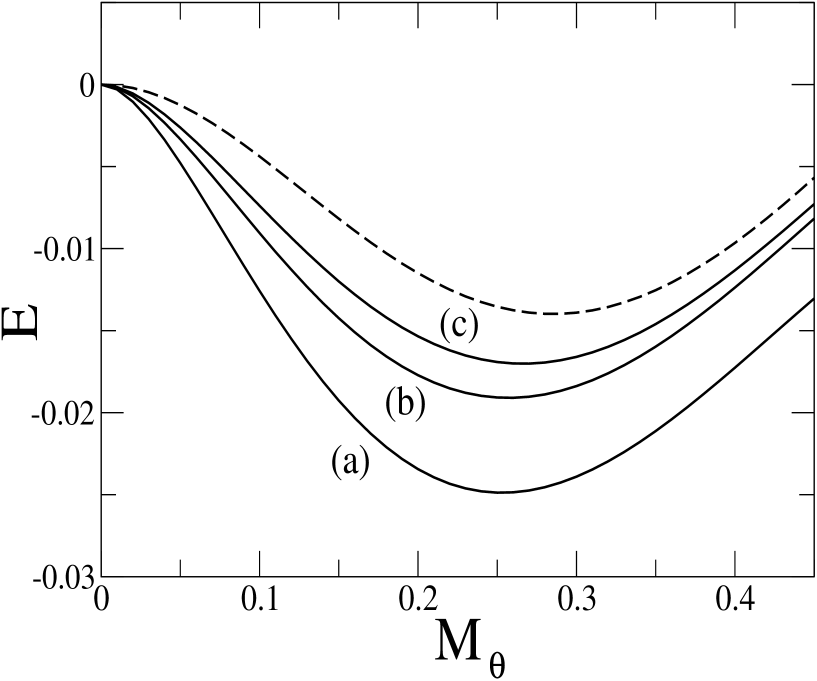
Figure 1: The energy density $E$ at $(\Lambda^{2}g/2\pi^{2})=2.5$ for the planar theory (dashed line) and for the noncommutative non-translational invariant case for $\theta\Lambda^{2}=12$ (a), $15$ (b), $18$ (c).

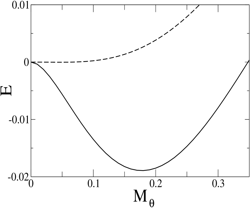
Figure 2: The energy density $E$ at $(\Lambda^{2}g/2\pi^{2})=2$ for the planar theory (dashed line) and for the noncommutative non-translational invariant case for $\theta\Lambda^{2}=8$ (solid line).

In both cases (static and non-static), the energy density difference between these two phases is of order $O(g/\theta^{4})$, while the difference with respect to the planar theory is much larger. Then, for convenience, in Figure 1 we plot $-\Gamma(G)/V$, in the non-static calculation, for the planar theory and for the non-translational invariant case, and in Figure 2 it is shown that the noncommutative effects decrease the critical coupling constant with respect to the planar GN model.

According to point i), one can easily evaluate the $x$ dependence of the vacuum condensate to order $O(1/\theta^{2})$, which turns out to be

$$<\bar{\psi}(x)\psi(x)>=\left(1+c\,P^{2}{\rm cos}\left(Px\right)\right)<\bar{\psi}\psi>_{TI}\;,$$ (42)

where $c$ is a constant and $<\bar{\psi}\psi>_{TI}$ is the constant order parameter evaluated in the translational invariant case.

V COMMENTS AND CONCLUSIONS

Our computation of the CJT effective action shows that the chiral symmetry breaking occurs for an inhomogeneous phase, due to the noncommutative nature of the four fermion interactions considered in Eq. (6). The energy difference between the inhomogeneous and the homogeneous phases, which both include the noncommutative corrections, is of order $O(g/\theta^{4})$. The order parameter has an oscillating $x$ dependence of order $O(g/\theta^{2})$, superposed to the constant background of the translational invariant phase.

These results are essentially based on the non-translational invariant ansatz for the full propagator in Eqs. (25) and (27). Let us notice that, in the commutative 1+1 dimensional GN model, non-translational invariant effects have been introduced in unopiu and a transition to the inhomogeneous crystal phase at non-zero chemical potential has been obtained.

In gubser ; noi for the noncommutative scalar case, it has been observed that the boson condensation does not occur in the mode $k=0$ but there is a total depletion to $k=Q$ where $<\phi(x)>\propto{\rm cos}(Qx)$. Analogously, in the fermionic case, our ansatz in Eq. (25) corresponds to Cooper pairs with a non-zero total momentum, as it happens in the LOFF phase in condensed matter. The latter point provides an indication that the noncommutative cutoff field theory could be applied to describe the features of the transition to inhomogeneous phases.

*

Appendix A A

In this Appendix we derive the energy for time, but not space translational invariant fermionic systems with Lagrangian given in Eq. (6), in terms of the static propagator $G(\vec{x},\vec{y})$ and we closely follow the procedure outlined in cjt for the scalar theory. The total energy is related to the effective action, computed in the static limit

$${\cal E}_{T}(G(\vec{x},\vec{y}))\tau=-\Gamma(G(x,y))|_{static}\;.$$ (43)

The static limit of the effective action is obtained by taking the time translational invariant propagator $G(x,y)=G(x_{0}-y_{0},\vec{x},\vec{y})$ at equal time $x_{0}=y_{0}$ and by re-expressing $\Gamma$ in terms of the static propagator, defined by the full propagator as $G(\vec{x},\vec{y})=G(0,\vec{x},\vec{y})$. To obtain the form of $G(\vec{x},\vec{y})$, we recall that the functional derivative of $\Gamma$ with respect to the propagator is related, as explained in detail in cjt , to the bilocal source $K(\vec{x},\vec{y})$

$$\frac{\delta\Gamma(\phi,G)}{\delta G(x_{0}-y_{0};\vec{x},\vec{y})}=-\frac{1}{2}\delta(x_{0}-y_{0})K(\vec{x},\vec{y})\;,$$ (44)

and therefore, from the explicit derivation of the effective action, one gets

$$G^{-1}(x,y)=-i\delta(x_{0}-y_{0})K(\vec{x},\vec{y})+S^{-1}\delta^{4}(x-y)+\frac{\delta\Gamma_{2}}{\delta G}\;,$$ (45)

which shows that the most general form of $G^{-1}(x,y)$ is

$$G^{-1}(x_{0}-y_{0},\vec{x},\vec{y})=\delta^{\prime}(x_{0}-y_{0})\gamma_{0}\delta(\vec{x}-\vec{y})+i\delta(x_{0}-y_{0})\vec{\gamma}\cdot\vec{f}(\vec{x},\vec{y})+im(\vec{x},\vec{y})\;,$$ (46)

where $\vec{f}(\vec{x},\vec{y})$ and $m(\vec{x},\vec{y})$ are generic functions of the spatial coordinates and all the dependence of $G^{-1}(x,y)$ on the temporal coordinates is contained in the delta function $\delta(x_{0}-y_{0})$ and its derivative . From Eq. (46) one gets the Fourier transform of $G^{-1}(x_{0}-y_{0},\vec{x},\vec{y})$ with respect to the variable $x_{0}-y_{0}$,

$${G}^{-1}(\omega,\vec{x},\vec{y})=\int_{-\infty}^{+\infty}\,dx_{0}e^{i\omega x_{0}}G^{-1}(x_{0},\vec{x},\vec{y})=-i\omega\gamma_{0}\delta(\vec{x}-\vec{y})+i\vec{\gamma}\cdot\vec{f}(\vec{x},\vec{y})+im(\vec{x},\vec{y})$$ (47)

which can be functionally inverted nota2 :

$${G}(\omega,\vec{x},\vec{y})=i\left(\frac{\omega\gamma_{0}-\vec{\gamma}\cdot\vec{f}+m}{\omega^{2}-F^{2}}\right)(\vec{x},\vec{y})\;,$$ (48)

where $F(\vec{x},\vec{y})=(f^{2}+m^{2})^{1/2}(\vec{x},\vec{y})$.

Finally, the static propagator is obtained by integration

$$G(\vec{x},\vec{y})=G(0,\vec{x},\vec{y})=$$

$$i\int\frac{\,d\omega}{2\pi}\left[\frac{\omega\gamma_{0}-\vec{\gamma}\cdot\vec{f}+m}{\omega^{2}-F^{2}}\right](\vec{x},\vec{y})=\frac{(\gamma_{0}F-\vec{\gamma}\cdot\vec{f}+m)}{2F}(\vec{x},\vec{y})\;.$$ (49)

Incidentally, we note that the trace over the spin indices gives

$${\rm Tr_{(spin)}}G(\vec{x},\vec{y})=\left(\frac{2m}{F}\right)(\vec{x},\vec{y})\;.$$ (50)

We are now able to evaluate the effective action in the static limit and, for simplicity, we shall restrict the following calculation to a constant mass $m(\vec{x},\vec{y})=m\delta(\vec{x}-\vec{y})$. We start considering the first term in the general expression of $\Gamma$ in Eq. (2), namely $-i{\rm Tr\,Ln}G^{-1}$, where the trace refers both to spacetime and spin indices (we neglect in Eq. (2) the logarithm of the free propagator $S$ which gives a constant contribution to the effective action). With the help of Eq. (47) one gets cjt

$$-i\int\,dx_{0}\int\,d^{3}x\int_{-\infty}^{+\infty}\frac{\,d\omega}{2\pi}{\rm Tr_{(spin)}\,Ln}({G}^{-1}(\omega,\vec{x},\vec{y}))=$$

$$-2i\int\,dx_{0}\int\,d^{3}x\int_{-\infty}^{+\infty}\frac{\,d\omega}{2\pi}{\rm Ln}(\omega^{2}-F^{2})=$$

$$2\int\,dx_{0}\int\,d^{3}x\,F(\vec{x},\vec{x})=4m\int\,dx_{0}\int\,d^{3}x[{\rm Tr_{(spin)}}G(\vec{x},\vec{x})]^{-1}\;,$$ (51)

where we have used Eq. (50) to replace $F$ in the last step.

The second term to compute in Eq. (2) is $-i{\rm Tr}S^{-1}G$ which yields, after integrating by parts,

$$-i\,{\rm Tr_{(spin)}}\int\,d^{4}x\,d^{4}y[/\partial\delta^{4}(x-y)]G(x_{0}-y_{0};\vec{x},\vec{y})=$$

$$i\,{\rm Tr_{(spin)}}\int\,d^{4}x\left[\left.\int\frac{\,d\omega}{2\pi}\gamma_{0}(-i\omega){G}(\omega,\vec{x},\vec{x})-\vec{\gamma}\vec{\nabla}G(0,\vec{x},\vec{y})\right|_{\vec{x}=\vec{y}}\right]=$$

$$-4m\int\,dx_{0}\int\,d^{3}{x}\,[{\rm Tr_{(spin)}}G(\vec{x},\vec{x})]^{-1}-\left.i{\rm Tr_{(spin)}}\int\,dx_{0}\int\,d^{3}{x}\,\vec{\gamma}\cdot\vec{\nabla}G(\vec{x},\vec{y})\right|_{\vec{x}=\vec{y}}\;.$$ (52)

Finally the term corresponding to $\Gamma_{2}$ in the Hartree-Fock approximation are straightforwardly computed by replacing $G(x_{0}-y_{0},\vec{x},\vec{y})|_{x_{0}=y_{0}}$ with $G(\vec{x},\vec{y})$. By collecting the various contributions to the effective action, namely Eqs. (51) and (52) plus $\Gamma_{2}$ in the Hartree-Fock approximation, we get the expression of the energy shown in Eq. (31).