Quantum Fluctuations of a Coulomb potential

Abstract

Long-range properties of the two-point correlation function of the electromagnetic field produced by an elementary particle are investigated. Using the Schwinger-Keldysh formalism it is shown that this function is finite in the coincidence limit outside the region of particle localization. In this limit, the leading term in the long-range expansion of the correlation function is calculated explicitly, and its gauge independence is proved. The leading contribution turns out to be of zero order in the Planck constant, and the relative value of the root mean square fluctuation of the Coulomb potential is found to be $1/\sqrt{2},$ confirming the result obtained previously within the S-matrix approach. It is shown also that in the case of a macroscopic body, the $\hbar^{0}$ part of the correlation function is suppressed by a factor $1/N\,,$ where $N$ is the number of particles in the body. Relation of the obtained results to the problem of measurability of the electromagnetic field is mentioned.

I Introduction

Fluctuations in the values of physical quantities is an inalienable trait of all quantum phenomena, which finds its reflection in the probabilistic nature of the quantum-mechanical description of elementary particle kinematics as well as of the field-theoretic treatment of the fundamental interactions. Investigation of fluctuations constitutes an essential part in establishing quasi-classical conditions, and therefore in dealing with the issue of correspondence between given quantum theory and its classical original.

Precise identification of the quasi-classical conditions is especially important in investigation of the measurement process. In this process, an essential role is played by the measuring device “recording” the results of an observation, and the question of primary importance is to what extent this device can be considered classically. Furthermore, investigation of fluctuations in the observable quantities themselves is a significant ingredient in the theoretical treatment of the measurement process, in particular, in verifying conformity of the formalism of quantum theory with the principal realizability of measurements.

In the latter aspect, the issue of quantum fluctuations of the electromagnetic field was considered in detail by Bohr and Rosenfeld bohr1 . In this classic paper, a comprehensive analysis of the measurability of electromagnetic field was given, and compatibility of the restrictions following from the formal relations for the field operators with the actual limitations inherent to any process of measurement was verified, refuting the earlier arguments by Landau and Peierls landau against this compatibility. In a subsequent paper bohr2 (see also rosenfeld ), the authors argued that the problem of charge-current measurements can be reduced to that already solved for the electromagnetic field. Later, a similar investigation was carried out in quantum theory of gravitation by DeWitt dewitt .

An important point underlying investigation of Refs. bohr1 ; bohr2 is that the question of measurability of the electromagnetic field, and hence of charges and currents, can be considered proceeding from the commutation relations for the operators describing free electromagnetic field. In particular, these relations were used to estimate characteristic value of the electromagnetic field fluctuations, denoted in bohr1 by $\mathfrak{S}.$ Defined as the root mean square fluctuation, $\mathfrak{S}$ is evidently of the order $O(\sqrt{\hbar}).$ It was argued in Ref. bohr1 that this estimate holds true even in the presence of sources, provided that the charge and current distributions representing these sources allow classical description (which was also confirmed later by detailed calculations in Refs. thirring ; glauber ; umezawa ; schwinger1 ).

As far as one is interested in the electromagnetic field produced by the test bodies, this result is certainly sufficient to justify the use of the relation $\mathfrak{S}=O(\sqrt{\hbar}):$ Since the choice of the experimental setup is at disposal of the observer, the measuring device may always be assumed “sufficiently classical.” However, the state of affairs is different when the given electromagnetic field to be measured is considered. Classical assumption about the field producing sources is irrelevant in this case, and the above estimate does not apply. The problem of fundamental importance, therefore, is to determine fluctuations of fields produced by nonclassical sources.

On various occasions, this issue has been the subject of a number of investigations. Electromagnetic field fluctuations springing up as a response of elementary particles’ vacua to external fields or nontrivial boundary conditions were studied recently in hacian ; barton ; eberlein ; ford1 ; zerbini where references to early works can be found. Fluctuations of the gravitational field, induced by vacuum fluctuations of the matter stress tensor were considered in Refs. zerbini ; ford2 ; ford3 ; hu1 ; hu2 .

It should be noted that despite extensive literature in the area, only vacua contributions of quantized matter fields to the fluctuations of electromagnetic and gravitational fields have been studied in detail. At the same time, it is effects produced by real matter that are most interesting from the point of view of the structure of elementary contributions to the field fluctuation.

The purpose of this paper is to investigate fluctuations of the electromagnetic field produced by a single massive charged particle, taking full account of quantum properties of the source-field interaction. It will be shown that the structure of fluctuations in this case is quite different from that of vacuum-induced fluctuations, or that found in the case of classical source. In particular, the root mean square fluctuation of the field turns out to be of zero order in the Planck constant, $\mathfrak{S}=O(\hbar^{0}),$ rather than $O(\sqrt{\hbar}).$ It seems that this remarkable fact has not been noticed earlier. For a given electric charge of the source consisting of many particles, the $\hbar^{0}$ contribution turns out to be inversely proportional to the number of constituent particles, so the classical $O(\sqrt{\hbar})$ estimate is recovered in the macroscopic limit.

The paper is organized as follows. In Sec. II a preliminary consideration of the problem is given, and the Schwinger-Keldysh closed time path formalism used throughout the work is briefly reviewed. General properties of the correlation function of electromagnetic field fluctuations are considered in Sec. III. In investigation of quantum aspects of particle-field interaction it is convenient to isolate purely quantum-mechanical effects related to the particle’s kinematics assuming it sufficiently heavy. As discussed in Sec. III.1, this leads naturally to the long-range expansion of the correlation function, making it appropriate to use the terminology and general ideas of effective field theories weinberg1 ; weinberg2 ; donoghue1 ; donoghue2 . Next, it is proved in Sec. III.2 that the leading term in the long-range expansion of the correlation function, which describes fluctuations of the static potential, is independent of the choice of gauge condition used to fix the gradient invariance. Finally, the correlation function is evaluated explicitly in Sec. IV. Sec. V contains discussion of the results obtained.

II Preliminaries

Let us consider a single particle with mass $m$ and electric charge $e.$ In classical theory, the electromagnetic field produced by such particle at rest is described by the Coulomb potential

$$A_{0}=\frac{e}{4\pi r}\,,\qquad\bm{A}=0\,.$$ (1)

Our aim is to determine properties of this potential in quantum domain. For this purpose, it is convenient to separate this field-theoretic problem from purely quantum mechanical issues related to the quantum kinematics of the particle. Namely, the particle’s mass will be assumed sufficiently large to neglect the indeterminacy in the values of particle velocity and position, following from the Heisenberg principle, so as to still be able to use the term “particle at rest.”

In quantum theory, Eq. (1) is reproduced by calculating the corresponding mean fields, $\langle\hat{A}_{0}\rangle,$ $\langle\hat{\bm{A}}\rangle.$ In the functional integral formalism, these are given by

$$\langle\hat{A}_{\mu}\rangle=\int\mathcal{D}\Phi A_{\mu}\exp\{iS\}\,,$$ (2)

where $\Phi$ collectively denotes the fundamental fields of the theory, $\Phi=\{A_{\mu},\phi,\phi^{*}\},$ the components $\phi,\phi^{*}$ describing the charged particle which for simplicity will be assumed scalar, $\mathcal{D}\Phi$ is the invariant integral measure, and $S=S[\Phi]$ the action functional of the system. Integration is carried over all field configurations satisfying

$$A^{\pm}\to 0\,,\quad\phi^{\pm}\to\phi_{0}^{\pm}\,,\quad(\phi^{*})^{\pm}\to(\phi_{0}^{*})^{\pm}\,,\qquad{\rm for}\quad t\to\mp\infty\,,$$

where the superscripts $+$ and $-$ denote the positive- and negative-frequency parts of the fields, respectively, and $\phi_{0}$ describes the particle state. Assuming that the gradient invariance of the theory is fixed by the Lorentz condition

$$G\equiv\partial^{\mu}A_{\mu}=0\,,$$ (3)

the action takes the form

$$S[\Phi] = S_{0}[\Phi]+S_{\rm gf}[\Phi]\,,$$

$$S_{0}[\Phi] = {\displaystyle\int}d^{4}x\left\{(\partial_{\mu}\phi^{*}+ieA_{\mu}\phi^{*})(\partial^{\mu}\phi-ieA^{\mu}\phi)-m^{2}\phi^{*}\phi\right\}-\frac{1}{4}{\displaystyle\int}d^{4}xF_{\mu\nu}F^{\mu\nu}\,,$$

$$S_{\rm gf}[\Phi] = -\frac{1}{2\xi}{\displaystyle\int}d^{4}x~{}G^{2}\,,\quad F_{\mu\nu}=\partial_{\mu}A_{\nu}-\partial_{\nu}A_{\mu}\,.$$ (4)

where $\xi$ is the Feynman weighting parameter. Introducing auxiliary classical sources $\mathcal{J}=\{J^{\mu},j^{*},j\}$ for the fields $\Phi=\{A_{\mu},\phi,\phi^{*}\},$ respectively, the right hand side of Eq. (2) may be rewritten in the standard way

$$\langle\hat{A}_{\mu}\rangle = \frac{\delta}{i\delta J^{\mu}}\exp\left\{S^{\rm{int}}\left[\frac{\delta}{i\delta\mathcal{J}}\right]\right\}\left.\int\mathcal{D}\Phi~{}\exp\left\{i\left(S^{(2)}+\int d^{4}x\left[J^{\mu}A_{\mu}+j\phi^{*}+j^{*}\phi\right]\right)\right\}\right|_{\mathcal{J}=0}$$ (5)

$$= \frac{\delta}{i\delta J^{\mu}}\exp\left\{S^{\rm{int}}\left[\frac{\delta}{i\delta\mathcal{J}}\right]\right\}\left.\exp\left\{i\int d^{4}x\int d^{4}y\left[\textstyle{\frac{1}{2}}J^{\mu}(x)D_{\mu\nu}(x,y)J^{\nu}(y)\right.\right.\right.$$

$$\left.\left.\left.+j^{*}(x)D(x,y)j(y)\right]+i\int d^{4}x~{}(j\phi_{0}^{*}+j^{*}\phi_{0})\right\}\right|_{\mathcal{J}=0}\,,$$

where $S^{(2)}$ denotes the free field part of the action, $S^{\rm{int}}[\Phi]=S[\Phi]-S^{(2)}[\Phi],$ $D_{\mu\nu}$ and $D$ are the propagators of the electromagnetic and scalar field, respectively, defined by

$$\int d^{4}z~{}\frac{\delta^{2}S^{(2)}}{\delta A^{\mu}(x)\delta A^{\nu}(z)}D^{\nu\alpha}(z,y) = -\delta_{\mu}^{\alpha}\delta^{(4)}(x-y)\,,$$ (6)

$$\int d^{4}z~{}\frac{\delta^{2}S^{(2)}}{\delta\phi^{*}(x)\delta\phi(z)}D(z,y) = -\delta^{(4)}(x-y)\,.$$ (7)

It is not difficult to verify that the result of evaluation of the right hand side of Eq. (5) in the tree approximation is given exactly by Eq. (1). The field fluctuation, however, cannot be determined just as directly. The point is that the formal expressions like $\langle\hat{A}_{0}^{2}(x)\rangle$ are not well defined because of the singular behavior of the product $\hat{A}_{0}(x)\hat{A}_{0}(y)$ as $x\to y.$ This is a well known problem, encountered already in the theory of free fields. As was emphasized in Ref. bohr1 , in any field measurement in a given spacetime point, one deals actually with the field averaged over a small but finite spacetime domain surrounding this point, so the physically sensible expression for the field operator is the following

$$\hat{\mathcal{A}}_{\mu}=\frac{1}{VT}\int_{T}dt\int_{V}d^{3}\bm{x}~{}\hat{A}_{\mu}(\bm{x},t)\,.$$ (8)

Respectively, the product of two fields in a given point is understood as the limit of

$$\hat{\mathcal{B}}_{\mu\nu}=\frac{1}{(VT)^{2}}\int_{T}dt\int_{T}dt^{\prime}\int_{V}d^{3}\bm{x}\int_{V}d^{3}\bm{x}^{\prime}~{}\hat{A}_{\mu}(\bm{x},t)\hat{A}_{\nu}(\bm{x}^{\prime},t^{\prime})$$ (9)

when the size of the domain tends to zero. Finally, the correlation function of the electromagnetic 4-potential in this domain is

$$\mathcal{C}_{\mu\nu}=\langle\hat{\mathcal{B}}_{\mu\nu}\rangle-\langle\hat{\mathcal{A}}_{\mu}\rangle\langle\hat{\mathcal{A}}_{\nu}\rangle\,.$$ (10)

The necessity of spacetime averaging of field operators, Eq. (8), dictated by the physical measurement conditions, entails the following important complication in calculating their correlation functions. The standard Feynman rules for constructing matrix elements of a product of field operators, such as that in the right hand side of Eq. (9), give the in-out matrix element of the time ordered product of the operators, i.e., the Green function, rather than its in-in expectation value. This circumstance is not essential as long as one is interested in evaluating (under stationary external conditions) the mean fields. However, it does make a difference in calculating the correlation function whether or not the field operators are smeared over a finite spacetime region. As is well known, in order to find the expectation value of a product of operators taken in different spacetime points, the usual Feynman rules for constructing the matrix elements must be modified. According to the so-called closed time path formalism keldysh ; schwinger2 (for modern reviews of the method, see Refs. jordan ; paz ), the in-in matrix element of the product $\hat{A}^{\mu}(x)\hat{A}^{\nu}(x^{\prime})$ can be written as

$$C^{\mu\nu}(x,x^{\prime}) \equiv \langle{\rm in}|\hat{A}^{\mu}(x)\hat{A}^{\nu}(x^{\prime})|{\rm in}\rangle$$ (11)

$$= \int\mathcal{D}\Phi_{-}\int\mathcal{D}\Phi_{+}~{}A^{\mu}_{-}(x)A^{\nu}_{+}(x^{\prime})\exp\{iS[\Phi_{+}]-iS[\Phi_{-}]\}\,,$$

where the subscript $+$ ($-$) shows that the time argument of the integration variable runs from $-\infty$ to $+\infty$ (from $+\infty$ to $-\infty$). Integration is over all fields satisfying

$$A^{+}_{\pm}\to 0\,,\quad\phi^{+}_{\pm}\to\phi_{0}^{+}\,,\quad(\phi^{*})^{+}_{\pm}\to(\phi^{*}_{0})^{+}\qquad{\rm for}\quad t \to -\infty\,,$$

$$\Phi_{+}=\Phi_{-}\qquad{\rm for}\quad t \to +\infty\,.$$ (12)

It is seen that $\langle{\rm in}|\hat{A}^{\mu}(x)\hat{A}^{\nu}(x^{\prime})|{\rm in}\rangle$ is given by the ordinary functional integral but with the number of fields doubled, and unusual boundary conditions specified above. Accordingly, diagrammatics generated upon expanding this integral in powers of the coupling constant $e$ consists of the following elements. There are four types of pairings for each field $A_{\mu}$ or $\phi,$ corresponding to the four different ways of placing two field operators on the two branches of the time path. They are conveniently combined into $2\times 2$ matrices

$$\mathfrak{D}^{\mu\nu}(x,y)=\left(\begin{array}[]{cc}D^{\mu\nu}_{++}(x,y)&D^{\mu\nu}_{+-}(x,y)\\ D^{\mu\nu}_{-+}(x,y)&D^{\mu\nu}_{--}(x,y)\end{array}\right)=\left(\begin{array}[]{cc}i\langle T\hat{A}^{\mu}(x)\hat{A}^{\nu}(y)\rangle_{0}&i\langle\hat{A}^{\nu}(y)\hat{A}^{\mu}(x)\rangle_{0}\\ i\langle\hat{A}^{\mu}(x)\hat{A}^{\nu}(y)\rangle_{0}&i\langle\tilde{T}\hat{A}^{\mu}(x)\hat{A}^{\nu}(y)\rangle_{0}\end{array}\right)\,,$$

$$\mathfrak{D}(x,y)=\left(\begin{array}[]{cc}D_{++}(x,y)&D_{+-}(x,y)\\ D_{-+}(x,y)&D_{--}(x,y)\end{array}\right)=\left(\begin{array}[]{cc}i\langle T\hat{\phi}(x)\hat{\phi}^{\dagger}(y)\rangle_{0}&i\langle\hat{\phi}(y)\hat{\phi}^{\dagger}(x)\rangle_{0}\\ i\langle\hat{\phi}(x)\hat{\phi}^{\dagger}(y)\rangle_{0}&i\langle\tilde{T}\hat{\phi}(x)\hat{\phi}^{\dagger}(y)\rangle_{0}\end{array}\right)\,,$$

where the operation of time ordering $T$ ($\tilde{T}$) arranges the factors so that the time arguments decrease (increase) from left to right, and $\langle\cdot\rangle_{0}$ denotes vacuum averaging. The “propagators” $\mathfrak{D}_{\mu\nu},$ $\mathfrak{D}$ satisfy the following matrix equations

$$\int d^{4}z~{}\mathfrak{G}_{\mu\nu}(x,z)\mathfrak{D}^{\nu\alpha}(z,y) = -\mathfrak{e}\delta_{\mu}^{\alpha}\delta^{(4)}(x-y)\,,\quad\mathfrak{G}_{\mu\nu}(x,y)=\mathfrak{i}~{}\frac{\delta^{2}S^{(2)}}{\delta A^{\mu}(x)\delta A^{\nu}(y)}\,,$$ (13)

$$\int d^{4}z~{}\mathfrak{G}(x,z)\mathfrak{D}(z,y) = -\mathfrak{e}\delta^{(4)}(x-y)\,,\quad\mathfrak{G}(x,y)=\mathfrak{i}~{}\frac{\delta^{2}S^{(2)}}{\delta\phi^{*}(x)\delta\phi(y)}\,,$$ (14)

where $\mathfrak{e},$ $\mathfrak{i}$ are $2\times 2$ matrices with respect to indices $+,-:$

$$\mathfrak{e}=\left(\begin{array}[]{cc}1&0\\ 0&1\end{array}\right)\,,\quad\mathfrak{i}=\left(\begin{array}[]{cc}1&0\\ 0&-1\end{array}\right)\,.$$

As in the ordinary Feynman diagrammatics of the S-matrix theory, the propagators are contracted with the vertex factors generated by the interaction part of the action, $S^{\rm int}[\Phi],$ with subsequent summation over $(+,-)$ in the vertices, each “$-$” vertex coming with an extra factor $(-1).$ This can be represented as the matrix multiplication of $\mathfrak{D}_{\mu\nu},\mathfrak{D}$ with suitable matrix vertices. For instance, the $A\partial\phi\phi^{*}$ part of the action generates the matrix vertex $\mathfrak{V}$ which in components has the form

$$V_{ijk}^{\mu}(x,y,z)=s_{ijk}\left.\frac{\delta^{3}S}{\delta A_{\mu}(x)\delta\phi(y)\delta\phi^{*}(z)}\right|_{\Phi=0}\,,$$

where the indices $i,j,k$ take the values $+,-,$ and $s_{ijk}$ is defined by $s_{+++}=-s_{---}=1$ and zero otherwise. External $\phi$ ($\phi^{*}$) line is represented in this notation by a column (row)

$$\mathfrak{r}=\left(\begin{array}[]{c}\phi_{0}\\ \phi_{0}\end{array}\right),\quad\mathfrak{r}^{\dagger}=(\phi^{*}_{0},\phi^{*}_{0}),$$

satisfying

$$\int d^{4}z~{}\mathfrak{G}(x,z)\mathfrak{r}(z)=\left(\begin{array}[]{c}0\\ 0\end{array}\right),\quad\int d^{4}x~{}\mathfrak{r}^{\dagger}(x)\mathfrak{G}(x,z)=(0,0)\,.$$ (17)

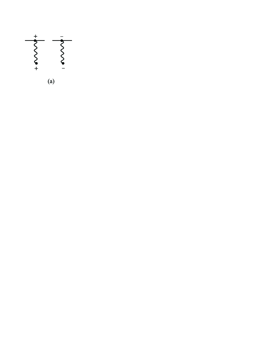
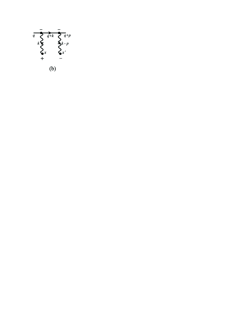
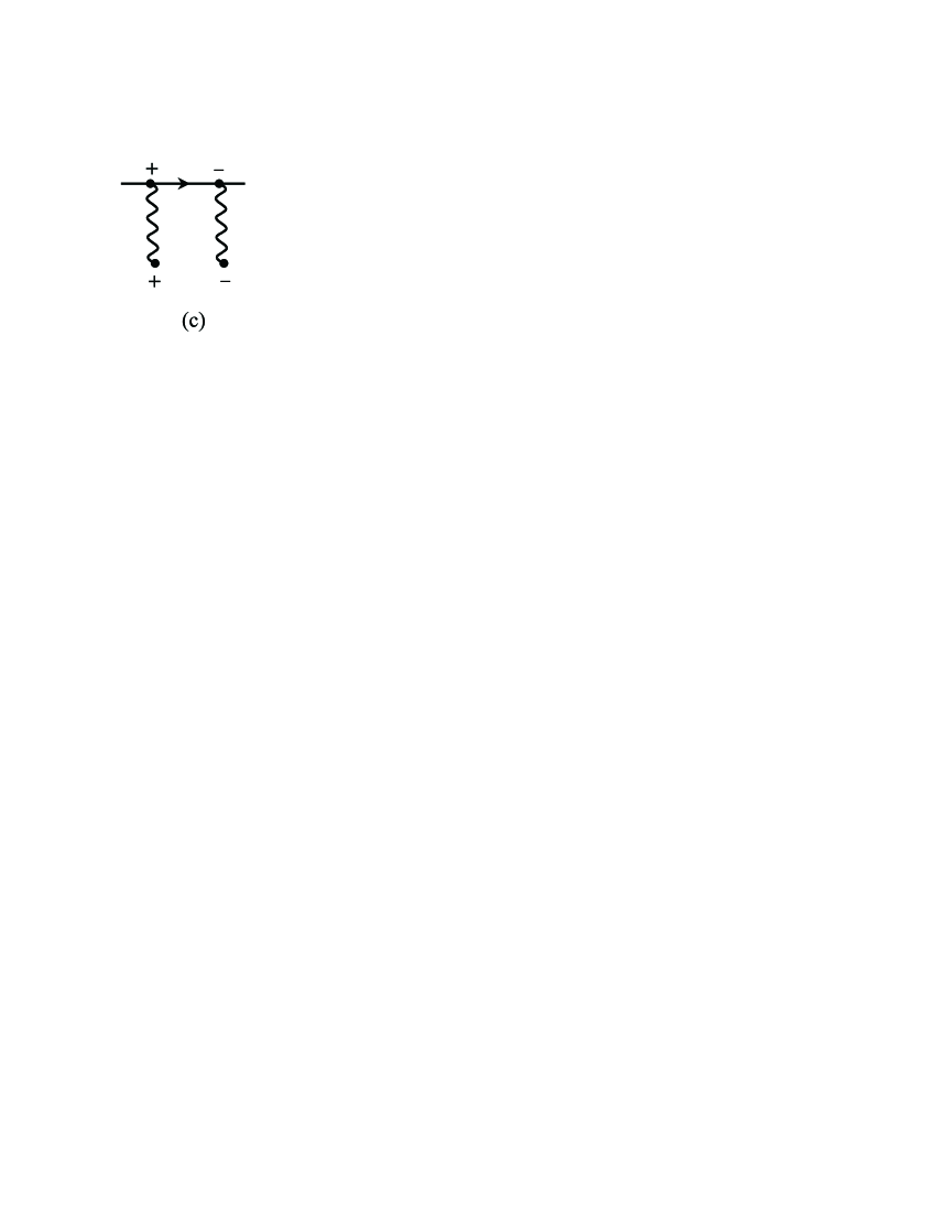
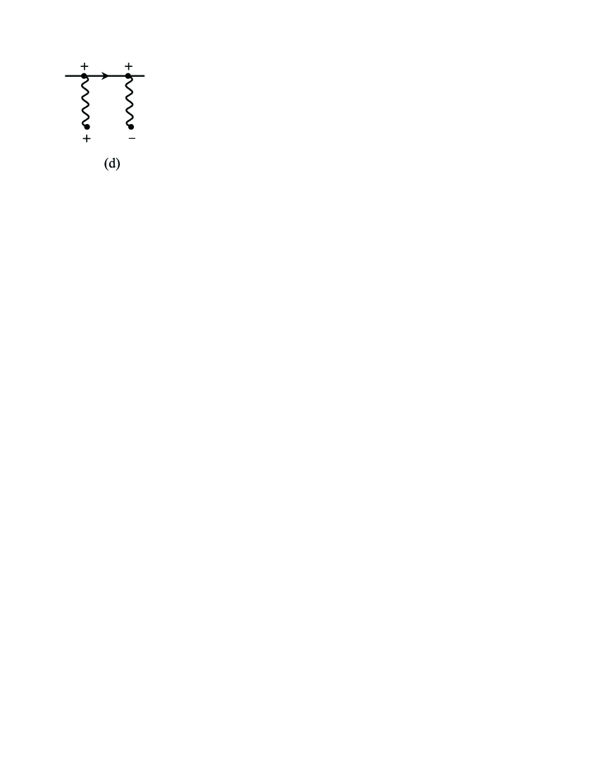
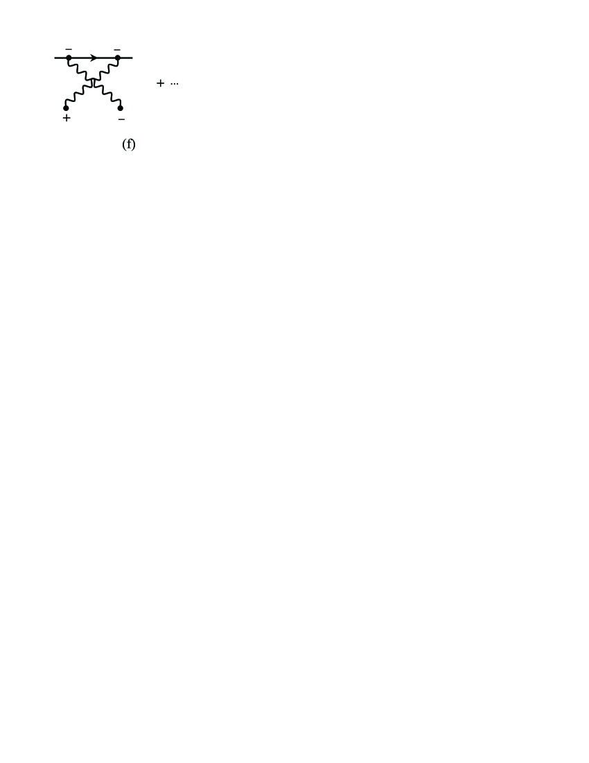
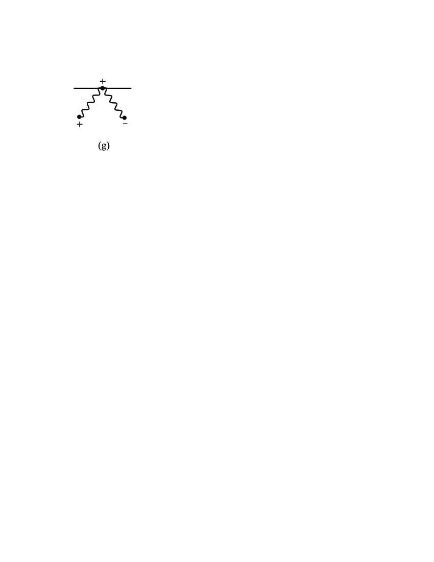
Figure 1: Tree contribution to the right hand side of Eq. (11). Wavy lines represent photon propagators, solid lines scalar particle. Part (f) of the figure represents the “transposition” of diagrams (b)–(e) (see Sec. IV).

Figure 1 depicts the tree diagrams contributing to the right hand side of Eq. (11). The disconnected part shown in Fig. 1(a) cancels in the expression for the correlation function [see Eq. (10)], which is thus represented by the diagrams (b)–(h).

Explicit expressions for various pairings of the photon and scalar fields

$$\mathfrak{D}_{\mu\nu} = \eta_{\mu\nu}\mathfrak{D}^{0}\,,\qquad\mathfrak{D}^{0}\equiv\mathfrak{D}|_{m=0}\,,$$

$$D_{++}(x,y) = \int\frac{d^{4}k}{(2\pi)^{4}}\frac{e^{-ik(x-y)}}{m^{2}-k^{2}-i0}\,,\quad D_{--}(x,y)=\int\frac{d^{4}k}{(2\pi)^{4}}\frac{e^{-ik(x-y)}}{k^{2}-m^{2}-i0}\,,$$

$$D_{-+}(x,y) = i\int\frac{d^{4}k}{(2\pi)^{3}}\theta(k^{0})\delta(k^{2}-m^{2})e^{-ik(x-y)}\,,\quad D_{+-}(x,y)=D_{-+}(y,x)\,.$$ (18)

The photon propagator is written here in the Feynman gauge $\xi=1$ which is most convenient in actual calculations. The question of how the choice of gauge condition affects the correlation function is considered in Sec. III.2.

III Long-range properties of correlation function

Before we proceed to calculation of the correlation function, we shall examine its general properties in more detail. Namely, the structure of the long-range expansion of the correlation function, and the question of its gauge dependence will be considered.

III.1 Correlation function in the long-range limit

The mean electromagnetic field produced by a massive charged particle is a function of five dimensional parameters - the fundamental constants $\hbar,c,$ the charge $e$ and mass $m$ of the particle, and the distance between the particle and the point of observation, $r.$ Of these only two independent dimensionless combinations can be constructed – the constant $e^{2}/\hbar c$ playing the role of the expansion parameter of perturbation theory, and the ratio $l_{c}/r\equiv\varkappa\,,$ where $l_{c}=\hbar/mc$ is the Compton length of the particle. As we have mentioned above, the particle is assumed sufficiently heavy so as to neglect effects related to the particle kinematics. This means that the quantum fluctuations are investigated in the limit $\varkappa\to 0.$ For fixed particle’s mass this implies large values of $r.$ In other words, the relevant information about field correlations is contained in the long-range behavior of the quantity $\mathcal{C}_{\mu\nu}.$

To extract this information we note, first of all, that in the long-range limit, the value of $\mathcal{C}_{\mu\nu}$ is independent of the choice of spacetime domain used in the definition of physical electromagnetic field operators, Eq. (8). Indeed, in any case the size of this domain must be small in comparison with the characteristic length at which the mean field changes significantly. In the case considered, this means that $V\ll r^{3}.$ To the leading order of the long-range expansion, therefore, the quantity $\langle\hat{A}_{\mu}(x)\hat{A}_{\nu}(x^{\prime})\rangle$ appearing in the right hand side of Eq. (10) can be considered constant within the domain. However, one cannot set $x=x^{\prime}$ in this expression directly. It is not difficult to see that the formal expression $\langle\hat{A}_{\mu}(x)\hat{A}_{\nu}(x)\rangle$ does not exist. Consider, for instance, the diagram 1(b). It is proportional to the integral

$$I_{\mu\nu}(x-x^{\prime},p)=\int d^{4}k\theta(k^{0})\delta(k^{2})e^{ik(x-x^{\prime})}\frac{(2q_{\mu}+k_{\mu}+p_{\mu})(2q_{\nu}+k_{\nu})}{[(k+q)^{2}-m^{2}](k-p)^{2}}\ ,$$

where $q_{\mu}$ is the 4-momentum of the scalar particle, and $p_{\mu}$ the momentum transfer. For small but nonzero $(x-x^{\prime})$ this integral is effectively cut-off at large $k$’s by the oscillating exponent, but for $x=x^{\prime}$ it is divergent. This divergence arises from integration over large values of virtual photon momenta, and therefore has nothing to do with the long-range behavior of the correlation function, because this behavior is determined by the low-energy properties of the theory. Evidently, the singularity of $I_{\mu\nu}(x-x^{\prime},p)$ for $x\to x^{\prime}$ is not worse than $\ln(x^{\mu}-x^{\prime\mu})^{2}/(x^{\mu}-x^{\prime\mu})^{2}.$ Therefore, $\langle{\rm in}|\hat{A}_{\mu}(x)\hat{A}_{\nu}(x^{\prime})|{\rm in}\rangle$ is integrable, and $\mathcal{C}_{\mu\nu}$ given by Eqs. (9), (10) is well defined.

Our aim below will be to show that this singularity can be consistently isolated and removed from the expression for $I_{\mu\nu}(x-x^{\prime},p)$ and similar integrals for the rest of diagrams in Fig. 1, without changing the long-range properties of the correlation function. After this removal, it is safe to set $x=x^{\prime}$ in the finite remainder, and to consider $\mathcal{C}_{\mu\nu}$ as a function of the single variable – the distance $r.$ An essential point of this procedure is that the singularity turns out to be local, and hence does not interfere with terms describing the long-range behavior, which guaranties unambiguity of the whole procedure.

It should be emphasized that in contrast to what takes place in the scattering theory, the ultraviolet divergences appearing in the course of calculation of the in-in matrix elements in the coincidence limit are generally non-polynomial with respect to the momentum transfer. The reason for this is the different analytic structure of various elements in the matrix propagators $\mathfrak{D}_{\mu\nu},$ $\mathfrak{D},$ which spoils the simple ultraviolet properties exhibited by the ordinary Feynman amplitudes. Take the above integral as an example. Because of the delta function in the integrand, differentiation of $I_{\mu\nu}(x-x^{\prime},p)$ with respect to the momentum transfer does not remove the ultraviolet divergence of $I_{\mu\nu}(0,p).$ What makes it all the more interesting is the result obtained in Sec. IV below, that the non-polynomial parts of divergent contributions eventually cancel each other, and the overall divergence turns out to be completely local.

Next, let us establish general form of the leading term in the long-range expansion of the correlation function. In momentum representation, an expression of lowest order in the momentum transfer with suitable dimension and Lorentz transformation properties is the following

$$\mathcal{C}^{(0)}_{\mu\nu}(p)\sim\frac{e^{2}}{m^{2}}\frac{q_{\mu}q_{\nu}}{\sqrt{-p^{2}}}\ .$$ (19)

Thus, only 00-component of the correlation function survives in the long-range limit:

$$\mathcal{C}^{(0)}_{00}(p)\sim\frac{e^{2}}{\sqrt{-p^{2}}}\ .$$

Not all diagrams of Fig. 1 contain contributions of this type. It is not difficult to identify those which do not. Consider, for instance, the diagram (h). It is proportional to the integral

$$\int d^{4}k\theta(k^{0})\delta(k^{2})\frac{e^{ik(x-x^{\prime})}}{(k-p)^{2}}\ ,$$

which does not involve the particle mass at all. Taking into account that each external scalar line gives rise to the factor $(2\varepsilon_{\bm{q}})^{-1/2},$ where $\varepsilon_{\bm{q}}=\sqrt{m^{2}+\bm{q}^{2}}\approx m\,,$ we see that the contribution of the diagram (h) is proportional to $1/m.$ The same is true of all other diagrams without internal scalar lines. As to diagrams involving such lines, it will be shown in Sec. IV by direct calculation that they do contain contributions of the type Eq. (19). But prior to this the question of their dependence on the gauge will be considered.

III.2 Gauge independence of the leading contribution

The value of 0-component of the momentum transfer is fixed by the mass shell condition for the scalar particle:

$$p^{0}=\sqrt{m^{2}+(\bm{p}+\bm{q})^{2}}-\sqrt{m^{2}+\bm{q}^{2}}=O\left(\frac{|\bm{p}|}{m}\right)\,.$$

It follows from this estimate that $p^{0}$ is to be set zero in the long-range limit. This implies that $\mathcal{C}^{(0)}_{\mu\nu}$ represents fluctuations in a quantity of direct physical meaning – the static potential energy of interacting particles. As such it is expected to be independent of the gauge condition used to fix the gradient invariance. More precisely, the issue of gauge dependence in the present case consists in the following. Although the gauge condition (3) fixes the form of the classical solution (1) unambiguously, the inverse is not true: There are infinitely many ways of constructing the gauge fixed action, which lead to the same expression for the static potential. We have to verify that this freedom in the choice of the gauge condition does not affect the value of $\mathcal{C}^{(0)}_{\mu\nu}.$

The gauge independence of the leading contribution will be demonstrated below in the most important particular case when changes of the gauge-fixed action are induced by variations of the Feynman weighting parameter $\xi.$ It is not difficult to see that these variations do not alter the value of classical potential. Indeed, the latter satisfies

$$\frac{\delta S_{\rm em}}{\delta A_{\mu}}=-J^{\mu}\,,$$ (20)

where $S_{\rm em}$ is the gauge-fixed action for electromagnetic field,

$$S_{\rm em}=-\frac{1}{4}{\displaystyle\int}d^{4}x\left(F_{\mu\nu}F^{\mu\nu}+\frac{2G^{2}}{\xi}\right)\,,$$

and $J^{\mu}$ the electromagnetic current,

$$J^{\mu}=ie\langle{\rm in}|\hat{\phi}^{\dagger}\partial^{\mu}\hat{\phi}-\hat{\phi}\partial^{\mu}\hat{\phi}^{\dagger}|{\rm in}\rangle\,.$$

Acting on Eq. (20) with $\partial_{\mu},$ using the current conservation $\partial_{\mu}J^{\mu}=0$ and the identity $\partial_{\mu}\partial_{\nu}F^{\mu\nu}=0,$ we obtain

$$\frac{1}{\xi}\Box G=0\,,$$

which implies that $G=0$ on the classical solution, and that $\xi$ effectively falls off from the classical equation (20). Let us now prove that $\mathcal{C}^{(0)}_{\mu\nu}$ remains unchanged under variations of $\xi$ too. We shall proceed along the lines of Ref. kazakov1 where $\xi$-independence of $\hbar^{0}$ part of the one-loop correction to Newtonian potential was proved within the S-matrix approach.

As we saw in Sec. III.1, the only diagrams contributing in the long-range limit are those containing internal scalar lines. We will show presently that the $\xi$-dependent part of these diagrams can be reduced to the form without such lines. First, it follows form Eq. (13) that the $\xi$-derivative of the electromagnetic propagator satisfies

$$\frac{\partial\mathfrak{D}_{\mu\nu}(x,y)}{\partial\xi}=\iint d^{4}zd^{4}z^{\prime}~{}\mathfrak{D}_{\mu\alpha}(x,z)\frac{\partial\mathfrak{G}^{\alpha\beta}(z,z^{\prime})}{\partial\xi}\mathfrak{D}_{\beta\nu}(z^{\prime},y)\,.$$ (21)

On the other hand, acting on Eq. (13) by $\partial^{\mu}$ one finds

$$\frac{1}{\xi}I\Box_{x}\partial_{x}^{\nu}\mathfrak{D}_{\nu\alpha}(x,y)=-E\partial^{x}_{\alpha}\delta^{(4)}(x-y)\,.$$ (22)

This equation can be resolved with respect to $\partial^{\nu}\mathfrak{D}_{\nu\alpha}.$ The reciprocal of the operator $I\Box,$ appropriate to the boundary conditions (II) is $(-\mathfrak{D}^{0}),$ hence

$$\partial_{x}^{\nu}\mathfrak{D}_{\nu\alpha}(x,y)=\xi\partial^{x}_{\alpha}\mathfrak{D}^{0}(x,y)\,.$$ (23)

Taking into account that

$$\frac{\partial\mathfrak{G}^{\alpha\beta}(z,z^{\prime})}{\partial\xi}=-\frac{I}{\xi^{2}}\partial_{z}^{\alpha}\partial_{z}^{\beta}\delta^{(4)}(z-z^{\prime})\,,$$

substituting this into Eq. (21), and using Eq. (23), we get

$$\frac{\partial\mathfrak{D}_{\mu\nu}(x,y)}{\partial\xi}=-\frac{1}{\xi}\int d^{4}z~{}\mathfrak{D}_{\mu\alpha}(x,z)I\partial_{z}^{\alpha}\partial^{z}_{\nu}\mathfrak{D}^{0}(z,y)\,,$$

or

$$\frac{\partial\mathfrak{D}_{\mu\nu}(x,y)}{\partial\xi}=\partial^{x}_{\mu}\partial^{y}_{\nu}\mathfrak{a}(x,y)\,,\qquad\mathfrak{a}(x,y)\equiv\int d^{4}z~{}\mathfrak{D}^{0}(x,z)I\mathfrak{D}^{0}(z,y)\,.$$ (24)

Thus, assuming the matrix indices and spacetime coordinates referring to the point of observation fixed, we see that the $\xi$-dependent part of the matrix photon propagator is contracted with the matrix vertex $\mathfrak{V}^{\mu}$ through a gradient term

$$\partial_{\mu}\mathfrak{b}(x)=\left(\begin{array}[]{c}\partial_{\mu}b_{+}(x)\\ \partial_{\mu}b_{-}(x)\end{array}\right)\,,\qquad\mathfrak{b}(x)=\partial^{y}_{\nu}\mathfrak{a}(x,y)\,.$$

Integrating by parts the spacetime derivative may be rendered to act on the vertex.

Next, we use gauge invariance of the action $S_{0}[\Phi]$ to transform $\mathfrak{b}\partial_{\mu}\mathfrak{V}^{\mu}.$ This invariance is expressed by the identity

$$\frac{\delta S_{0}}{\delta\phi(x)}ie\phi(x)-\frac{\delta S_{0}}{\delta\phi^{*}(x)}ie\phi^{*}(x)-\partial^{x}_{\mu}\frac{\delta S_{0}}{\delta A_{\mu}(x)}=0\,.$$ (25)

Differentiating Eq. (25) twice with respect to $\phi,\phi^{*},$ and setting $\Phi=0$ gives

$$\left.\partial^{x}_{\mu}\frac{\delta^{3}S_{0}}{\delta A_{\mu}(x)\delta\phi(y)\delta\phi^{*}(z)}\right|_{\Phi=0} = \frac{\delta^{2}S^{(2)}_{0}}{\delta\phi^{*}(z)\delta\phi(x)}ie\delta^{(4)}(x-y)-\frac{\delta^{2}S^{(2)}_{0}}{\delta\phi(y)\delta\phi^{*}(x)}ie\delta^{(4)}(x-z)\,.$$ (26)

The matrix vertex $\mathfrak{V}^{\mu}$ is obtained by multiplying $\delta^{3}S_{0}/\delta\phi\delta\phi^{*}\delta A_{\mu}$ by the matrix $s_{ijk}.$ It follows from Eq. (26) that the combination $\mathfrak{b}\partial_{\mu}\mathfrak{V}^{\mu}$ may be written as

$$b_{i}\partial^{x}_{\mu}V_{ijk}^{\mu}(x,y,z) = ie(b_{+}s_{+jk}+b_{-}s_{-jk})\left\{\frac{\delta^{2}S^{(2)}_{0}}{\delta\phi^{*}(z)\delta\phi(x)}\delta^{(4)}(x-y)-\frac{\delta^{2}S^{(2)}_{0}}{\delta\phi(y)\delta\phi^{*}(x)}\delta^{(4)}(x-z)\right\},$$

or

$$\mathfrak{b}\partial^{x}_{\mu}\mathfrak{V}^{\mu}(x,y,z)=ie\left\{\mathfrak{F}(z,x)\delta^{(4)}(x-y)-\mathfrak{F}(x,y)\delta^{(4)}(x-z)\right\}\,,$$ (27)

where

$$\mathfrak{F}(x,y)=\mathfrak{f}~{}\frac{\delta^{2}S^{(2)}_{0}}{\delta\phi^{*}(x)\delta\phi(y)}\,,\qquad\mathfrak{f}=\left(\begin{array}[]{cc}b_{+}&0\\ 0&-b_{-}\end{array}\right)\,.$$

Finally, contracting $\mathfrak{b}\partial_{\mu}\mathfrak{V}^{\mu}(x,y,z)$ with the matrix $\mathfrak{D}(y,y^{\prime})$ and the vector $\tilde{\mathfrak{r}}(z)=\left(\phi_{0}(z),\phi_{0}(z)\right)\,,$ and using Eqs. (14), (17) gives

$$\iint d^{4}yd^{4}z~{}\tilde{\mathfrak{r}}(z)\mathfrak{b}\partial^{x}_{\mu}\mathfrak{V}^{\mu}(x,y,z)\mathfrak{D}(y,y^{\prime}) = ie\int d^{4}z~{}\tilde{\mathfrak{r}}(z)\mathfrak{F}(z,x)~{}\mathfrak{D}(x,y^{\prime})$$

$$-ie\tilde{\mathfrak{r}}(x)\int d^{4}y\mathfrak{F}(x,y)\mathfrak{D}(y,y^{\prime}) = ie\phi_{0}\tilde{\mathfrak{b}}\delta^{(4)}(x-y^{\prime})\,.$$

We see that upon extracting the $\xi$-dependent part of the diagrams (b)–(f) in Fig. 1, the scalar propagator is cancelled by the vertex factor. Using the reasoning of Sec. III.1, the resulting diagrams give rise to terms $\sim 1/m\,.$ Thus, $\xi$-independence of the correlation function in the long-range limit is proved.

IV Evaluation of the leading contribution

Let us proceed to calculation of the leading contribution to the correlation function. It is contained in the sum of diagrams (b)–(f) in Fig. 1, which has the symbolic form

$$C_{\mu\nu}=I_{\mu\nu}+I^{\rm tr}_{\mu\nu}\,,\qquad I_{\mu\nu}=\frac{1}{i}\left\{\mathfrak{D}_{\mu\alpha}\left[\mathfrak{r}^{\dagger}\mathfrak{V}^{\alpha}\mathfrak{D}\mathfrak{V}^{\beta}\mathfrak{r}\right]\mathfrak{D}_{\beta\nu}\right\}_{+-}\,,$$

where the superscript “tr” means transposition of the indices and spacetime arguments referring to the points of observation: $\mu\leftrightarrow\nu,$ $+\leftrightarrow-,$ $x\leftrightarrow x^{\prime}$ [the transposed contribution is represented by the diagrams collected in part (f) of Fig. 1]. As it follows from the considerations of Sec. III.1, $\mathcal{C}^{(0)}_{\mu\nu}$ can be expressed through $C_{\mu\nu}$ as

$$\mathcal{C}^{(0)}_{\mu\nu}=\lim\limits_{\genfrac{}{}{0.0pt}{}{m\to\infty}{V,T\to 0}}\left\{\frac{1}{(VT)^{2}}\iint\limits_{(V,T)}d^{4}xd^{4}x^{\prime}~{}C_{\mu\nu}(x,x^{\prime})\right\}\,.$$ (28)

Written longhand, $I_{\mu\nu}$ reads

$$I_{\mu\nu}(x,x^{\prime})=ie^{2}\iint d^{4}zd^{4}z^{\prime}\Biggl{\{} + D^{0}_{++}(x,z)\left[\phi^{*}(z)\stackrel{{\scriptstyle\leftrightarrow}}{{\partial_{\mu}}}D_{++}(z,z^{\prime})\stackrel{{\scriptstyle\leftrightarrow}}{{\partial_{\nu}^{\,\prime}}}\phi(z^{\prime})\right]D^{0}_{+-}(z^{\prime},x^{\prime})$$

$$- D^{0}_{++}(x,z)\left[\phi^{*}(z)\stackrel{{\scriptstyle\leftrightarrow}}{{\partial_{\mu}}}D_{+-}(z,z^{\prime})\stackrel{{\scriptstyle\leftrightarrow}}{{\partial_{\nu}^{\,\prime}}}\phi(z^{\prime})\right]D^{0}_{--}(z^{\prime},x^{\prime})$$

$$- D^{0}_{+-}(x,z)\left[\phi^{*}(z)\stackrel{{\scriptstyle\leftrightarrow}}{{\partial_{\mu}}}D_{-+}(z,z^{\prime})\stackrel{{\scriptstyle\leftrightarrow}}{{\partial_{\nu}^{\,\prime}}}\phi(z^{\prime})\right]D^{0}_{+-}(z^{\prime},x^{\prime})$$

$$+ D^{0}_{+-}(x,z)\left[\phi^{*}(z)\stackrel{{\scriptstyle\leftrightarrow}}{{\partial_{\mu}}}D_{--}(z,z^{\prime})\stackrel{{\scriptstyle\leftrightarrow}}{{\partial_{\nu}^{\,\prime}}}\phi(z^{\prime})\right]D^{0}_{--}(z^{\prime},x^{\prime})\Biggr{\}}\,,$$

where

$$\varphi\stackrel{{\scriptstyle\leftrightarrow}}{{\partial_{\mu}}}\psi=\varphi\partial_{\mu}\psi-\psi\partial_{\mu}\varphi\,.$$

Contribution of the third term in the right hand side of Eq. (IV) is zero identically. Indeed, using Eq. (II), and performing spacetime integrations we see that the three lines coming, say, into $z$-vertex are all on the mass shell, which is inconsistent with the momentum conservation in the vertex. The remaining terms in Eq. (IV) take the form

$$I_{\mu\nu}(x,x^{\prime}) = e^{2}\iint\frac{d^{3}\bm{q}}{(2\pi)^{3}}\frac{d^{3}\bm{p}}{(2\pi)^{3}}\frac{a^{*}(\bm{q})a(\bm{q}+\bm{p})}{\sqrt{2\varepsilon_{\bm{q}}2\varepsilon_{{\bm{q}}+\bm{p}}}}e^{-ipx^{\prime}}\tilde{I}_{\mu\nu}(p,q)\,,\quad p_{0}=\varepsilon_{\bm{q}+\bm{p}}-\varepsilon_{\bm{q}}\,,$$ (30)

where

$$\tilde{I}_{\mu\nu}(p,q)=-i\int\frac{d^{4}k}{(2\pi)^{4}} e^{-ik(x-x^{\prime})}(2q_{\mu}+k_{\mu})(2q_{\nu}+k_{\nu}+p_{\nu})$$

$$\times\Bigl{\{} \;\;D^{0}_{++}(k)D_{++}(q+k)D^{0}_{+-}(k-p)$$ (31)

$$-D^{0}_{++}(k)D_{+-}(q+k)D^{0}_{--}(k-p)$$

$$+D^{0}_{+-}(k)D_{--}(q+k)D^{0}_{--}(k-p) \Bigr{\}}\,,$$

and $a(\bm{q})$ is the Fourier transform of the particle wave function, normalized by

$$\int\frac{d^{3}\bm{q}}{(2\pi)^{3}}|a(\bm{q})|^{2}=1\,.$$

The function $a(\bm{q})$ is generally of the form

$$a(\bm{q})=b(\bm{q})e^{-i\bm{q}\bm{x}_{0}},$$

where $\bm{x}_{0}$ is the mean particle position, and $b(\bm{q})$ is such that

$$\int d^{3}\bm{q}~{}b(\bm{q})e^{i\bm{qx}}=0$$ (32)

for $\bm{x}$ outside of some finite region $W$ around $\bm{x}=0.$

Upon extraction of the leading contribution these expressions considerably simplify. First of all, one has $\varepsilon_{\bm{q}+\bm{p}}\approx\varepsilon_{\bm{q}}\approx m,$ and hence, $p_{0}\approx 0.$ Next, $b(\bm{q}+\bm{p})$ may be substituted by $b(\bm{q}):$ This implies that we disregard spatial spreading of the wave packet, neglecting the multipole moments of the charge distribution. Taking into account the normalization condition, Eq. (30) thus becomes

$$I_{\mu\nu}(x,x^{\prime}) = \frac{e^{2}}{2m}\iint\frac{d^{3}\bm{q}}{(2\pi)^{3}}\frac{d^{3}\bm{p}}{(2\pi)^{3}}|b(\bm{q})|^{2}e^{i\bm{p}(\bm{x^{\prime}}-\bm{x}_{0})}\tilde{I}_{\mu\nu}(p,q)\,,\quad p_{0}=0\,.$$ (33)

The leading term in $\tilde{I}_{\mu\nu}(p,q)$ has the form [Cf. Eq. (19)]

$$\tilde{I}^{(0)}_{\mu\nu}(p,q)\sim\frac{e^{2}}{m^{2}}\frac{q_{\mu}q_{\nu}}{\sqrt{-p^{2}}}\ .$$ (34)

This singular at $p\to 0$ contribution comes from integration over small $k$ in Eq. (IV). Therefore, to the leading order, the momenta $k,p$ in the vertex factors can be neglected in comparison with $q.$ Thus,

$$\tilde{I}_{\mu\nu}(p,q)=-4q_{\mu}q_{\nu}i\int\frac{d^{4}k}{(2\pi)^{4}}e^{-ik(x-x^{\prime})}\Bigl{\{} D^{0}_{++}(k)D_{++}(q+k)D^{0}_{+-}(k-p)$$ (35)

$$- D^{0}_{++}(k)D_{+-}(q+k)D^{0}_{--}(k-p)$$

$$+ D^{0}_{+-}(k)D_{--}(q+k)D^{0}_{--}(k-p)\Bigr{\}}\,.$$

Furthermore, it is convenient to combine various terms in this expression with the corresponding terms in the transposed contribution. Noting that the right hand side of Eq. (35) is explicitly symmetric in $\mu,\nu,$ and that the variables $x,x^{\prime}$ in the exponent can be freely interchanged because they appear symmetrically in Eq. (28), we may write

$$\tilde{C}_{\mu\nu}(p,q) \equiv \tilde{I}_{\mu\nu}(p,q)+\tilde{I}^{\rm tr}_{\mu\nu}(p,q)=-4q_{\mu}q_{\nu}i\int\frac{d^{4}k}{(2\pi)^{4}}e^{-ik(x-x^{\prime})}$$

$$\times\Bigl{\{} \left[D^{0}_{++}(k)D_{++}(q+k)D^{0}_{+-}(k-p)+D^{0}_{--}(k)D_{--}(q+k)D^{0}_{-+}(k-p)\right]$$ (36)

$$+ \left[D^{0}_{+-}(k)D_{--}(q+k)D^{0}_{--}(k-p)+D^{0}_{-+}(k)D_{++}(q+k)D^{0}_{++}(k-p)\right]$$

$$- \left[D^{0}_{++}(k)D_{+-}(q+k)D^{0}_{--}(k-p)+D^{0}_{--}(k)D_{-+}(q+k)D^{0}_{++}(k-p)\right]\Bigr{\}}\,.$$

With the help of the relation

$$D_{--}+D_{++}=D_{+-}+D_{-+}\,,$$ (37)

which is a consequence of the identity

$$T\hat{\phi}(x)\hat{\phi}(y)+\tilde{T}\hat{\phi}(x)\hat{\phi}(y)-\hat{\phi}(x)\hat{\phi}(y)-\hat{\phi}(y)\hat{\phi}(x)=0\,,$$

the first term in the integrand can be transformed as

$$D^{0}_{++}(k)D_{++}(q+k)D^{0}_{+-}(k-p)+D^{0}_{--}(k)D_{--}(q+k)D^{0}_{-+}(k-p)$$

$$=D^{0}_{++}(k)D_{++}(q+k)D^{0}(k-p)+D^{0}(k)D_{--}(q+k)D^{0}_{-+}(k-p)\,,$$

where

$$D(k)\equiv D_{+-}(k)+D_{-+}(k)=2\pi i\delta(k^{2}-m^{2})\,,\quad D^{0}(k)=D(k)|_{m=0}\,.$$

Here we used the already mentioned fact that $D^{0}_{+-}(k)D_{-+}(k+q)\equiv 0$ for $q$ on the mass shell. Analogously, the second term becomes

$$D^{0}(k)D_{--}(q+k)D^{0}_{--}(k-p)-D^{0}_{-+}(k)D_{--}(q+k)D^{0}(k-p)\,.$$

Changing the integration variables $k\to k+p,$ $\bm{q}\to\bm{q}-\bm{p},$ and then $\bm{p}\to-\bm{p},$ noting that the leading term is even in the momentum transfer [see Eq. (34)], and that $\bm{p}(\bm{x}-\bm{x}^{\prime})$ in the exponent can be omitted in the coincidence limit ($x\to x^{\prime}$), the sum of the two terms takes the form

$$D^{0}(k)\left[D_{++}(q+k)D^{0}_{++}(k-p)+D_{--}(q+k)D^{0}_{--}(k-p)\right]\,.$$

Similar transformations of the rest of the integrand yield

$$D^{0}_{++}(k)D_{+-}(q+k)D^{0}_{--}(k-p)+D^{0}_{--}(k)D_{-+}(q+k)D^{0}_{++}(k-p)$$

$$\to-\frac{1}{2}\left[D^{0}_{++}(k)D(q+k)D^{0}_{++}(k-p)+D^{0}_{--}(k)D(q+k)D^{0}_{--}(k-p)\right]\,.$$ (38)

Substituting these expressions into Eq. (IV) and using Eq. (II) gives

$$\tilde{C}_{\mu\nu}(p,q) = 4q_{\mu}q_{\nu}\int\frac{d^{4}k}{(2\pi)^{3}}e^{-ik(x-x^{\prime})}$$ (39)

$$\times {\rm Re}\left\{\frac{2\delta(k^{2})}{[(k-p)^{2}+i0][(q+k)^{2}-m^{2}+i0]}+\frac{\delta[(q+k)^{2}-m^{2}]}{[k^{2}+i0][(k-p)^{2}+i0]}\right\}\,.$$

As was discussed in Sec. III.1, the exponent in the integrand in Eq. (39) plays the role of an ultraviolet cutoff, ensuring convergence of the integral at large $k$’s. On the other hand, the leading contribution (34) is determined by integrating over $k\sim p$ where it is safe to take the limit $x\to x^{\prime}.$ Since $(x-x^{\prime})$ is eventually set equal to zero, one can further simplify the $k$ integral by using the dimensional regulator instead of the oscillating exponent. Namely, introducing the dimensional regularization of the $k$ integral, one may set $x=x^{\prime}$ afterwards to obtain

$$\tilde{C}_{\mu\nu}(p,q) = 4q_{\mu}q_{\nu}\mu^{\epsilon}~{}{\rm Re}\int\frac{d^{4-\epsilon}k}{(2\pi)^{3}}\left\{\frac{2\delta(k^{2})}{[(k-p)^{2}+i0][(q+k)^{2}-m^{2}+i0]}\right.$$ (40)

$$+ \left.\frac{\delta[(q+k)^{2}-m^{2}]}{[k^{2}+i0][(k-p)^{2}+i0]}\right\}\,,$$

where $\mu$ is an arbitrary mass parameter, and $\epsilon=4-d,$ $d$ being the dimensionality of spacetime.

Next, going over to the $\alpha$-representation, the first term in the integrand may be parameterized as

$$\frac{\delta(k^{2})}{[(k-p)^{2}+i0][(q+k)^{2}-m^{2}+i0]}=\frac{\delta(k^{2})}{(p^{2}-2kp+i0)(2kq+i0)}$$

$$=\frac{1}{2\pi i^{2}}\iiint_{0}^{\infty}dxdydz\left(e^{ixk^{2}}+e^{-ixk^{2}}\right)e^{iy(p^{2}-2kp+i0)}e^{iz(2kq+i0)}$$ (41)

Substituting this into Eq. (40), and using the formulas

$$\int d^{4-\epsilon}k~{}e^{i(ak^{2}+2bk)}={\rm sign}(a)\frac{1}{i}\left(\frac{\pi}{|a|}\right)^{2-\epsilon/2}\exp\left(\frac{b^{2}}{ia}\right),$$

$$\int_{0}^{\infty}dx~{}x^{-\epsilon}e^{ixa}=i~{}\Gamma(1-\epsilon)\exp\left({\rm sign}(a)\frac{\pi\epsilon}{2i}\right)\frac{|a|^{\epsilon}}{a}\,,$$

one finds

$$K(p) \equiv \mu^{\epsilon}\int\frac{d^{4-\epsilon}k}{(2\pi)^{3}}\frac{\delta(k^{2})}{[(k-p)^{2}+i0][(q+k)^{2}-m^{2}]}$$

$$= \frac{i\mu^{\epsilon}}{(2\pi)^{4}}\iiint_{0}^{\infty}dxdydz\left(\frac{\pi}{x}\right)^{2-\epsilon/2}e^{iyp^{2}}\left\{\exp\left[-\frac{i}{x}(yp-zq)^{2}\right]-\exp\left[\frac{i}{x}(yp-zq)^{2}\right]\right\}$$

$$= \frac{\mu^{\epsilon}\pi^{-\epsilon/2}}{8\pi^{2}}\cos\left(\frac{\pi\epsilon}{4}\right)\Gamma\left(1-\frac{\epsilon}{2}\right)\iint_{0}^{\infty}dydz~{}e^{iyp^{2}}\frac{\left|(yp-zq)^{2}\right|^{\epsilon/2}}{(yp-zq)^{2}}\,.$$

Changing the integration variable $z\to yz,$ and taking into account that $q^{2}=m^{2},$ $qp=-p^{2}/2$ yields

$$K(p) = \frac{(\mu m)^{\epsilon}\pi^{-\epsilon/2}}{8\pi^{2}m^{2}}\cos\left(\frac{\pi\epsilon}{4}\right)\Gamma\left(1-\frac{\epsilon}{2}\right)\int_{0}^{\infty}dy~{}e^{iyp^{2}}y^{\epsilon-1}\int_{0}^{\infty}dz\frac{\left|z^{2}-(1+z)\alpha\right|^{\epsilon/2}}{z^{2}-(1+z)\alpha}$$ (42)

$$= \frac{(\pi e^{i\pi})^{-\epsilon/2}}{8\pi^{2}m^{2}}\left(\frac{\mu m}{-p^{2}}\right)^{\epsilon}\cos\left(\frac{\pi\epsilon}{4}\right)\Gamma\left(1-\frac{\epsilon}{2}\right)\Gamma(\epsilon)\int_{0}^{\infty}dz~{}\frac{\left|z^{2}-(1+z)\alpha\right|^{\epsilon/2}}{z^{2}-(1+z)\alpha}\ ,$$

where $\alpha\equiv-p^{2}/m^{2}\,.$ Similar manipulations with the second term in Eq. (40) give

$$L(p) \equiv \mu^{\epsilon}\int\frac{d^{4-\epsilon}k}{(2\pi)^{3}}\frac{\delta[(q+k)^{2}-m^{2}]}{[k^{2}+i0][(k-p)^{2}+i0]}=-\frac{\mu^{\epsilon}}{(2\pi)^{4}}\iiint_{0}^{\infty}dxdydz$$

$$\times \int d^{4-\epsilon}k\left(e^{ix(k^{2}+2kq)}+e^{-ix(k^{2}+2kq)}\right)e^{iy(p^{2}-2k(q+p)+i0)}e^{iz(-2kq+i0)}$$

$$= \frac{i\mu^{\epsilon}}{(2\pi)^{4}}\iiint_{0}^{\infty}dxdydz\left(\frac{\pi}{x}\right)^{2-\epsilon/2}e^{iyp^{2}}\left\{\exp\left[-\frac{i}{x}((x-z)q-y(q+p))^{2}\right]\right.$$

$$- \left.\exp\left[\frac{i}{x}((x+z)q+y(q+p))^{2}\right]\right\}=\frac{\pi^{-\epsilon/2}}{16\pi^{2}m^{2}}\left(\frac{\mu}{m}\right)^{\epsilon}\Gamma\left(1+\frac{\epsilon}{2}\right)$$

$$\times \iint_{0}^{\infty}dydz\left\{\frac{e^{i\pi\epsilon/4}}{[(y+z+1)^{2}+yz\alpha]^{1+\epsilon/2}}+\frac{e^{-i\pi\epsilon/4}}{[(y+z-1)^{2}+yz\alpha]^{1+\epsilon/2}}\right\}\,.$$

Changing the integration variables $y=ut,$ $z=(1-u)t$ yields

$$L(p) = \frac{\pi^{-\epsilon/2}}{16\pi^{2}m^{2}}\left(\frac{\mu}{m}\right)^{\epsilon}\Gamma\left(1+\frac{\epsilon}{2}\right)$$

$$\times \int_{0}^{\infty}dt\int_{0}^{1}du~{}t\left\{\frac{e^{i\pi\epsilon/4}}{[(t+1)^{2}+u(1-u)t^{2}\alpha]^{1+\epsilon/2}}+\frac{e^{-i\pi\epsilon/4}}{[(t-1)^{2}+u(1-u)t^{2}\alpha]^{1+\epsilon/2}}\right\}\,.$$

On the other hand, $L(p)$ must be real because the poles of the functions $D_{++}(k),$ $D_{++}(k-p)$ actually do not contribute. Hence,

$$L(p) = \frac{\pi^{-\epsilon/2}}{8\pi^{2}m^{2}}\left(\frac{\mu}{m}\right)^{\epsilon}\cos\left(\frac{\pi\epsilon}{4}\right)\Gamma\left(1+\frac{\epsilon}{2}\right)\int_{0}^{\infty}dt\int_{0}^{1}\frac{t~{}du}{[(t+1)^{2}+u(1-u)t^{2}\alpha]^{1+\epsilon/2}}\ .$$

Let us turn to investigation of singularities of the expressions obtained when $\epsilon\to 0.$ Evidently, both $K(p)$ and $L(p)$ contain single poles

$$K_{\rm div}(p) = \frac{1}{8\pi^{2}m^{2}\epsilon}~{}\mathchoice{{\vbox{\hbox{$\textstyle-$}}\kern-4.86108pt}}{{\vbox{\hbox{$\scriptstyle-$}}\kern-3.25pt}}{{\vbox{\hbox{$\scriptscriptstyle-$}}\kern-2.29166pt}}{{\vbox{\hbox{$\scriptscriptstyle-$}}\kern-1.875pt}}\!\int_{0}^{\infty}\frac{dz}{z^{2}-(1+z)\alpha}=-\frac{1}{8\pi^{2}m^{2}\epsilon}\frac{1/\alpha}{\sqrt{1+4/\alpha}}\ln\frac{\sqrt{1+4/\alpha}+1}{\sqrt{1+4/\alpha}-1}\ ,$$

$$L_{\rm div}(p) = \frac{1}{8\pi^{2}m^{2}\epsilon}~{}\int_{0}^{1}\frac{du}{[1+u(1-u)\alpha]}=\frac{1}{4\pi^{2}m^{2}\epsilon}\frac{1/\alpha}{\sqrt{1+4/\alpha}}\ln\frac{\sqrt{1+4/\alpha}+1}{\sqrt{1+4/\alpha}-1}\ .$$ (43)

Note that $L_{\rm div}=-2K_{\rm div}.$ Upon substitution into Eq. (40) the pole terms cancel each other. Thus, $\tilde{C}_{\mu\nu}(p,q)$ turns out to be finite in the limit $\epsilon\to 0.$ Taking into account also that divergences of the remaining two diagrams (g), (h) in Fig. 1 are independent of the momentum transfer, we conclude that the singular part of the correlation function is completely local.

It is worth of mentioning that although the quantity $K_{\rm div}(p)$ is non-polynomial with respect to $p^{2},$ signifying non-locality of the corresponding contribution to $C_{\mu\nu}(x,x^{\prime}),$ it is analytic at $p=0,$ which implies that its Fourier transform is local to any finite order of the long-range expansion. Indeed, expansion of $K_{\rm div}(p)$ around $\alpha=0$ reads

$$K_{\rm div}(p) = -\frac{1}{16\pi^{2}m^{2}\epsilon}\left(1-\frac{\alpha}{6}+\cdots+\frac{(-1)^{n}(n!)^{2}}{(2n+1)!}\alpha^{n}+\cdots\right)\,.$$ (44)

Contribution of such term to $C_{\mu\nu}(x,x^{\prime})$ is proportional to

$$\int\frac{d^{3}\bm{p}}{(2\pi)^{3}}e^{i\bm{p}(\bm{x^{\prime}}-\bm{x}_{0})}\left(1-\frac{\alpha}{6}+\cdots\right)=\delta^{(3)}(\bm{x^{\prime}}-\bm{x}_{0})+\frac{1}{6m^{2}}\triangle\delta^{(3)}(\bm{x^{\prime}}-\bm{x}_{0})+\cdots\,.$$

The delta function arose here because we neglected spacial spreading of the wave packet. Otherwise, we would have obtained

$$\iint\frac{d^{3}\bm{q}}{(2\pi)^{3}}\frac{d^{3}\bm{p}}{(2\pi)^{3}}b^{*}(\bm{q})b(\bm{q}+\bm{p})e^{i\bm{p}(\bm{x^{\prime}}-\bm{x}_{0})}\left(1-\frac{\alpha}{6}+\cdots\right)=0\quad{\rm for}\quad\bm{x^{\prime}}-\bm{x}_{0}\notin W\,,$$

as a consequence of the condition (32). In particular, applying this to the correlation function, we see that its divergent part does not contribute outside of $W.$ Thus, the two-point correlation function has a well defined coincidence limit everywhere except the region of particle localization.

Turning to calculation of the finite part of $K(p),$ we subtract the divergence from the right hand side of Eq. (IV), and set $\epsilon=0$ afterwards:

$$K_{\rm fin}(p)\equiv\lim\limits_{\epsilon\to 0}\bigl{[}K(p)-K_{\rm div}(p)\bigr{]}$$

$$=\frac{1}{16\pi^{2}m^{2}}\Biggl{\{}-\left[i\pi+\ln\pi+\gamma+2\ln\left(\frac{-p^{2}}{\mu m}\right)\right]\mathchoice{{\vbox{\hbox{$\textstyle-$}}\kern-4.86108pt}}{{\vbox{\hbox{$\scriptstyle-$}}\kern-3.25pt}}{{\vbox{\hbox{$\scriptscriptstyle-$}}\kern-2.29166pt}}{{\vbox{\hbox{$\scriptscriptstyle-$}}\kern-1.875pt}}\!\int_{0}^{\infty}\frac{dz}{z^{2}-(1+z)\alpha}$$

$$+~{}\mathchoice{{\vbox{\hbox{$\textstyle-$}}\kern-4.86108pt}}{{\vbox{\hbox{$\scriptstyle-$}}\kern-3.25pt}}{{\vbox{\hbox{$\scriptscriptstyle-$}}\kern-2.29166pt}}{{\vbox{\hbox{$\scriptscriptstyle-$}}\kern-1.875pt}}\!\int_{0}^{\infty}dz~{}\frac{\ln\left|z^{2}-(1+z)\alpha\right|}{z^{2}-(1+z)\alpha}\Biggr{\}}\ ,$$ (45)

where $\gamma$ is the Euler constant. The leading contribution is contained in the last integral. Extracting it with the help of Eq. (51) of the Appendix, we find

$$K^{(0)}_{\rm fin}(p)=\frac{1}{64m\sqrt{-p^{2}}}\,.$$ (46)

As to $L(p),$ it does not contain the root singularity. Indeed,

$$L(0)=\frac{\pi^{-\epsilon/2}}{8\pi^{2}m^{2}}\left(\frac{\mu}{m}\right)^{\epsilon}\cos\left(\frac{\pi\epsilon}{4}\right)\frac{\Gamma\left(1+\epsilon/2\right)}{\epsilon(1+\epsilon)}\,,$$

and therefore $L_{\rm fin}(p)\equiv\lim\limits_{\epsilon\to 0}[L(p)-L_{\rm div}(p)]$ is finite at $p=0.$ It is not difficult to verify that $L_{\rm fin}(p)$ is in fact analytic at $p=0.$ Thus, substituting Eq. (46) into Eqs. (40), (33), and then into Eq. (28), and using the formula

$$\int\frac{d^{3}\bm{p}}{(2\pi)^{3}}\frac{e^{i\bm{px}}}{|\bm{p}|} = \frac{1}{2\pi^{2}\bm{x}^{2}}\,,$$

we finally arrive at the following expression for the leading long-range contribution to the correlation function

$$\mathcal{C}_{00}^{(0)}(x)=\frac{e^{2}}{32\pi^{2}r^{2}}\ ,\qquad r=|\bm{x}-\bm{x}_{0}|\,,$$ (47)

all other components of $\mathcal{C}^{(0)}_{\mu\nu}$ vanishing. This result coincides with that obtained by the author in the framework of the S-matrix approach kazakov3 . The root mean square fluctuation of the Coulomb potential turns out to be

$$\sqrt{\left\langle A^{2}_{0}(r)\right\rangle}=\frac{e}{\sqrt{32}\,\pi r}\,.$$ (48)

Note also that the relative value of the fluctuation is $1/\sqrt{2}.$ It is interesting to compare this value with that obtained for vacuum fluctuations. As was shown in Ref. zerbini , the latter is equal to $\sqrt{2}$ (this is the square root of the relative variance $\Delta^{2}_{r}$ used in Ref. zerbini ).

We can now ask for conditions to be imposed on a system in order to allow classical consideration of its electromagnetic interactions. Such a condition can easily be found out by examining dependence of the $\hbar^{0}$ contribution on the number of field producing particles. Let us consider a body with total electric charge $Q$ and mass $M,$ consisting of a large number $N=Q/q$ of elementary particles with charge $q$ and mass $m,$ assumed identical for simplicity. Then it is readily seen that the diagrams (b)–(f) in Fig. 1 are proportional to $N\cdot q^{2}=Q^{2}/N\,$ because they have only two external matter lines. We conclude that the $\hbar^{0}$ contribution to the correlation function, given for an elementary particle by Eq. (47), turns into zero in the macroscopic limit $N\to\infty.$ At the same time, the next term in the long-range expansion of the correlation function has the form

$$\mathcal{C}^{(1)}\sim\frac{e^{2}}{m}\frac{\hbar}{cr^{3}}\,.$$

Hence, for a fixed mass $M$ of the multi-particle body, it is independent of $N,$

$$\mathcal{C}^{(1)}\sim N\frac{(Q/N)^{2}}{(M/N)}\frac{\hbar}{cr^{3}}=\frac{Q^{2}}{M}\frac{\hbar}{cr^{3}}\,,$$

thus recovering the classical estimate $\mathfrak{S}=O(\sqrt{\hbar})$ in the macroscopic limit.

V Discussion and conclusions

The main result of the present work is the expression (48) describing quantum fluctuations of the electrostatic potential of a charged particle. It represents the leading contribution in the long-range expansion, and is valid at distances much larger than the Compton length of the particle. Remarkably, the fluctuation turns out be zero order in the Planck constant. This result is obtained by evaluating two-point correlation function of the electromagnetic 4-potential in the coincidence limit. We have shown that despite non-locality of divergences arising in various diagrams in this limit, the total divergent part of the in-in matrix element is local, and hence does not contribute outside the region where the particle is localized.

Perhaps, it is worth to stress once more that the issue of locality of divergences is only a technical aspect of our considerations. This locality does make the structure of the long-range expansion transparent and comparatively simple. However, even if the divergence were nonlocal this would not present a principal difficulty. A physically sensible definition of an observable quantity always includes averaging over a finite spacetime domain, while the singularity of the two-point function, occurring in the coincidence limit, is integrable (see Sec. III.1). The only problem with the nonlocal divergence would be impossibility to take the limit of vanishing size of the spacetime domain [Cf. Eq. (28)].

Turning back to the problem of measurability of electromagnetic field, which served as the starting point of our investigation, we may conclude that the proof of principal realizability of measurements, given in Refs. bohr1 ; bohr2 , is incomplete, since it relies heavily on the $O(\sqrt{\hbar})$ estimate for the electromagnetic field fluctuations, which is inapplicable to the fields of elementary particles. The latter case therefore requires further investigation.

As we saw in the end of Sec. IV, the $\hbar^{0}$ contribution to the correlation function of the electromagnetic field of a macroscopic body is suppressed by the factor $1/N.$ This is in agreement with the necessary condition for neglecting the $\hbar^{0}$ contribution, formulated in Ref. kazakov2 in connection with the loop corrections to the post-Newtonian expansion in general relativity. In the present context, it coincides with the well-known criterion for neglecting quantum fluctuations tomboulis ; callan ; zerbini .

Appendix A

In the course of separation of the finite part in the right hand side of Eq. (IV) we encountered the integral

$$A\equiv\mathchoice{{\vbox{\hbox{$\textstyle-$}}\kern-4.86108pt}}{{\vbox{\hbox{$\scriptstyle-$}}\kern-3.25pt}}{{\vbox{\hbox{$\scriptscriptstyle-$}}\kern-2.29166pt}}{{\vbox{\hbox{$\scriptscriptstyle-$}}\kern-1.875pt}}\!\int_{0}^{\infty}dz~{}\frac{\ln\left|z^{2}-(1+z)\alpha\right|}{z^{2}-(1+z)\alpha} = \mathchoice{{\vbox{\hbox{$\textstyle-$}}\kern-4.86108pt}}{{\vbox{\hbox{$\scriptstyle-$}}\kern-3.25pt}}{{\vbox{\hbox{$\scriptscriptstyle-$}}\kern-2.29166pt}}{{\vbox{\hbox{$\scriptscriptstyle-$}}\kern-1.875pt}}\!\int_{0}^{\infty}dz~{}\frac{\ln\left|(z-p_{1})(z-p_{2})\right|}{(z-p_{1})(z-p_{2})}\,,$$

$$p_{1,2} = \frac{\alpha\pm\sqrt{\alpha^{2}+4\alpha}}{2}\,.$$

To evaluate this integral, let us consider the integral

$$\bar{A}=\int_{C}dw~{}\frac{\ln[(w-p_{1})(w-p_{2})]}{(w-p_{1})(w-p_{2})}\ ,$$ (49)

taken over the contour $C$ in the complex $w$ plane, shown in Fig. 2. $\bar{A}$ is zero identically. On the other hand, one has for sufficiently small positive $\sigma$

$$\bar{A}=\int_{-\infty}^{p_{1}-\sigma}dz~{}\frac{\ln[(z-p_{1})(z-p_{2})]}{(z-p_{1})(z-p_{2})}-i\pi\frac{\ln(p_{2}-p_{1})}{p_{1}-p_{2}}-\frac{i\pi\ln\sigma+\pi^{2}/2}{p_{1}-p_{2}}$$

$$+\int_{p_{1}+\sigma}^{p_{2}-\sigma}dz~{}\frac{\ln[(z-p_{1})(p_{2}-z)]-i\pi}{(z-p_{1})(z-p_{2})}-i\pi\frac{\ln(p_{2}-p_{1})-i\pi}{p_{2}-p_{1}}-\frac{i\pi\ln\sigma+\pi^{2}/2}{p_{2}-p_{1}}$$

$$+\int_{p_{2}+\sigma}^{\infty}dz~{}\frac{\ln[(z-p_{1})(z-p_{2})]-2i\pi}{(z-p_{1})(z-p_{2})}\,.$$

Changing the integration variable $z\to(p_{1}+p_{2})-z$ in the first integral, and rearranging yields in the limit $\sigma\to 0$

$$A=\frac{1}{2}\int_{0}^{p_{1}+p_{2}}dz~{}\frac{\ln[(p_{2}-z)(z-p_{1})]}{(z-p_{1})(z-p_{2})}+\frac{\pi^{2}/2}{p_{2}-p_{1}}\,.$$ (50)

The root singularity is contained in the second term, because

$$\int_{0}^{p_{1}+p_{2}}dz~{}\frac{\ln[(p_{2}-z)(z-p_{1})]}{(z-p_{1})(z-p_{2})}\to-\ln\alpha\quad{\rm for}\quad\alpha\to 0.$$

Thus,

$$A^{\rm root}=\frac{\pi^{2}}{4\sqrt{\alpha}}\,.$$ (51)

It is interesting to note also that the part containing the root singularity [the second term in Eq. (50)] exactly coincides with that found using the S-matrix (Cf. Eq. (B2) in Ref. kazakov3 ).

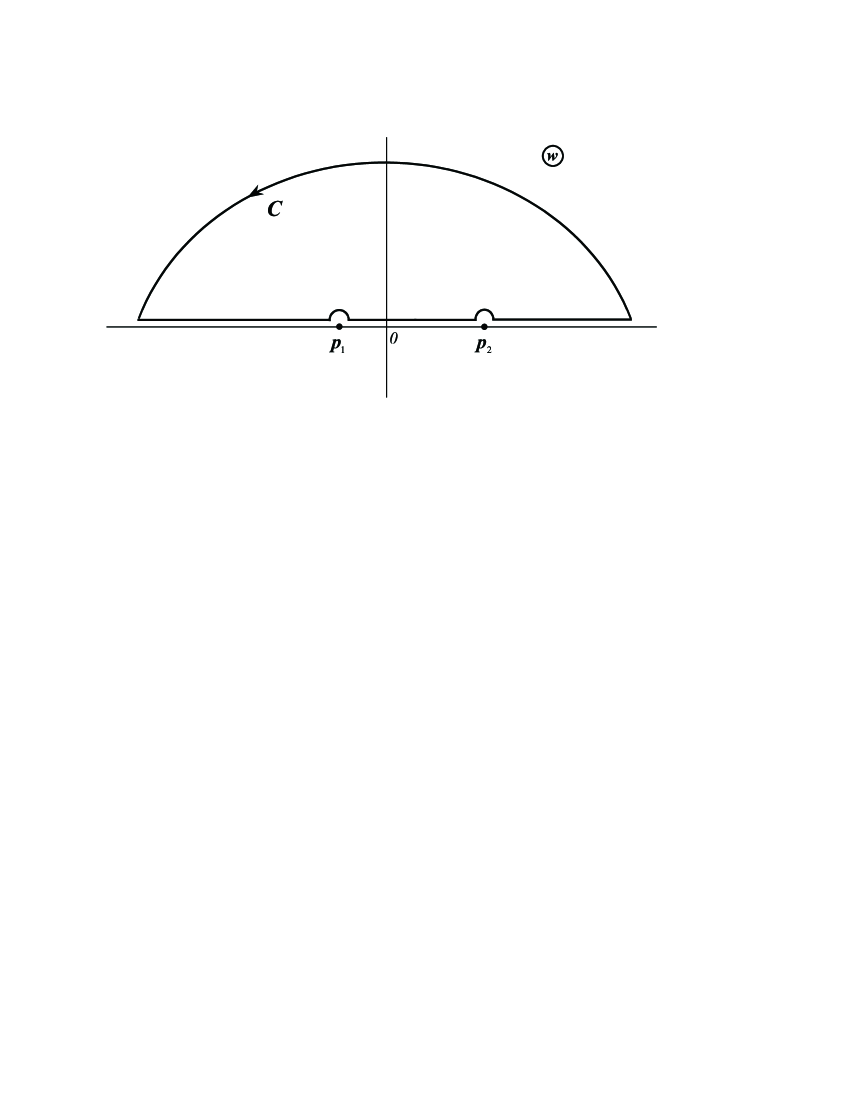
Figure 2: Contour of integration in Eq. (49).

References

- (1) N. Bohr and L. Rosenfeld, Kgl. Danske Vidensk. Selskab., Math.-Fys. Medd. 12, 3 (1933).
- (2) L. D. Landau and R. Peierls, Zs. f. Phys. 69, 56 (1931).
- (3) N. Bohr and L. Rosenfeld, Phys. Rev. 78, 794 (1950).
- (4) L. Rosenfeld, On quantum electrodynamics, in: Niels Bohr and the development of physics, ed. W. Pauli (London, 1955) p. 114.
- (5) B. S. DeWitt, The quantization of geometry, in: Gravitation: an introduction to current research, ed. L. Witten (Wiley, New-York, 1962) p. 266.
- (6) W. Thirring and B. Touschek, Phil. Mag. 62, 244 (1951).
- (7) R. Glauber, Phys. Rev. 84, 395 (1951).
- (8) H. Umezawa, Y. Takahashi, and S. Kamefuchi, Phys. Rev. 85, 505 (1951).
- (9) J. Schwinger, Phys. Rev. 91, 728 (1953).
- (10) S. Hacian, R. Jauregui, F. Soto, and C. Villarreal, J. Phys. A23, 2401 (1990).
- (11) G. Barton, J. Phys. A: Math. Gen. 24, 991 (1991); 24, 5533 (1991).
- (12) C. Eberlein, J. Phys. A: Math. Gen. 25, 3015 (1992); 25, 3038 (1992).
- (13) L. H. Ford, Phys. Rev. D47, 5571 (1993).
- (14) G. Cognola, E. Elizalde, and S. Zerbini, Phys. Rev. D65, 085031 (2002).
- (15) Chung-I Kuo and L. H. Ford, Phys. Rev. D47, 4510 (1993).
- (16) L. H. Ford, Phys. Rev. D51, 1692 (1995).
- (17) B. L. Hu and A. Matacz, Phys. Rev. D51, 1577 (1995).
- (18) N. G. Phillips and B. L. Hu, Phys. Rev. D55, 6123 (1997).
- (19) S. Weinberg, Physica (Amsterdam) 96A, 327 (1979).
- (20) H. Leutwyler and S. Weinberg, in: Proc. of the XXVIth Int. Conf. on High Energy Physics, ed. J. Sanford (Dallas, TX, 1992), AIP Conf. Proc. No. 272 (AIP, NY, 1993) pp. 185, 346.
- (21) J. F. Donoghue, in: Effective Field Theories of the Standard Model, ed. U.-G. Meissner (World Scientific, Singapore, 1994).
- (22) J. F. Donoghue, Phys. Rev. Lett. 72, 2996 (1994); Phys. Rev. D50, 3874 (1994).
- (23) J. Schwinger, J. Math. Phys. 2, 407 (1961); Particles, Sources and Fields (Addison-Wesley, Reading, Mass., 1970).
- (24) L. V. Keldysh, Zh. Eksp. Teor. Fiz. 47, 1515 (1964) [Sov. Phys. JETP 20, 1018 (1965)].
- (25) R. D. Jordan, Phys. Rev. D33, 444 (1986); 36, 3593 (1987).
- (26) J. P. Paz, Phys. Rev. D41, 1054 (1990).
- (27) K. A. Kazakov, Phys. Rev. D66, 044003 (2002).
- (28) K. A. Kazakov, “Quantum fluctuations of effective fields and the correspondence principle,” hep-th/0207218.
- (29) K. A. Kazakov, Class. Quantum Grav. 18, 1039 (2001); Nucl. Phys. Proc. Suppl. 104, 232 (2002); Int. J. Mod. Phys. D12, 1715 (2003).
- (30) E. Tomboulis, Phys. Lett. B70, 361 (1977).
- (31) C. G. Callan,Jr., S. B. Giddings, J. A. Harvey, and A. Strominger, Phys. Rev. D45, 1005 (1992).