Gauge theories on hyperbolic spaces
and dual wormhole instabilities

hep-th/0402174

February 2004

1 Introduction

Diffeomorphism invariance of a gravitational theory implies that classical backgrounds related by coordinate transformations are physically equivalent. This is no longer the case once quantum effects are taken into account. The reason is simply because different space-like foliations of the background geometry lead to different definitions of a time ( and thus a Hamiltonian) of a quantum system. This has profound implications for the gauge theory/string theory correspondence [2]. In the simplest case, the holographic correspondence of Maldacena relates ${\cal N}=4$ $SU(N)$ supersymmetric Yang-Mills (SYM) theory in $R^{3,1}$ and type IIB supergravity in $AdS_{5}\times S^{5}$, where $AdS_{5}$ is written in Poincare’ patch coordinates. As emphasized in [3], even though classical (Euclidean) $AdS_{5}$ foliations by $R^{4},\ S^{4},\ H_{4}$ are related by coordinate transformations, the corresponding gauge theories are physically inequivalent. This is so because a classical supergravity background (in the large $N$ limit, and for the large ’t Hooft gauge theory coupling) is equivalent to the full quantum gauge theory on the corresponding slices. The correspondence between gauge theories on curved space-times and gravitational duals becomes more involved for nonconformal gauge theories [3, 4, 5, 6, 7, 8, 9].

Quite intriguing, certain supergravity backgrounds holographic to gauge theories on negatively curved space-times are represented by wormhole solutions [8, 9]. As stressed in [9], existence of multiple boundaries in these Euclidean supergravity solutions makes it difficult to establish a detailed dictionary for the gauge/string theory correspondence. Moreover, the negative curvature of the supergravity boundary leads to a nonperturbative instability due to the $D3\overline{D3}$ pair production [10]. The latter suggests that wormhole solutions arising in this construction are somewhat unphysical, and should disappear once nonperturbative instabilities are removed. In this paper we study nonperturbative instabilities of strongly coupled four dimensional gauge theories on smooth compact quotients of hyperbolic spaces, and existence of non-perturbatively stable Euclidean supergravity wormholes representing their holographic dual.

Since instabilities on the supergravity side are associated with the tachyonic modes of the dual gauge theory, the natural way to eliminate them is to remove tachyons from the gauge theory spectrum. The gauge theory tachyons come from conformally coupled scalars, which were massless prior to introducing background space-time curvature. Indeed, an effective potential for such a scalar $\phi$ is

$$V_{\phi}=\frac{1}{12}\ R_{4}\ \phi^{2}\,,$$ (1.1)

giving rise to a negative mass square $m^{2}_{\phi}={\textstyle{\frac{1}{6}}}R_{4}$ for negative 4d Ricci scalar curvature $R_{4}$. These scalars are ’true’ tachyons only when the spacial directions of the gauge theory background are compactified. This is also the case with the instabilities on the supergravity side: they are present only for compact spatial directions. In the noncompact case, say $H_{4}$ of radius $L$, the mass of a conformally coupled scalar is above the Breitenlohner-Freedman bound

$$m^{2}_{\phi}=-\frac{2}{L^{2}}\qquad>\qquad m_{BF}^{2}=-\frac{9}{4L^{2}}\,,$$ (1.2)

and thus does not lead to any instabilities. Similarly, in this case the potential barrier to create a $D3\overline{D3}$ pair in the dual supergravity background is infinite, simply because $H_{4}$ volume is infinite. For this reason, we consider four-dimensional gauge theories on $S^{1}\times\Sigma_{3}$ and $\Sigma_{4}$, where $\Sigma_{n}$ is a smooth, compact, finite volume quotient of a hyperbolic space $H_{n}$ by a discrete subgroup $\Gamma$ of its $SO(n,1)$ symmetry group, $\Sigma_{n}=H_{n}/\Gamma$.

In the next section we study $D3$ probe brane dynamics in supergravity dual to ${\cal N}=4$ $SU(N)$ SYM theory on $S^{1}\times\Sigma_{3}$, which is a Euclidean continuation of this gauge theory on $R\times\Sigma_{3}$ at finite temperature. The motivation to study this potential mechanism for lifting tachyonic modes comes from finite temperature field theory intuition: there, a thermal mass can be induced to lift otherwise tachyonic mode. We find that the instability still persists. In fact, no thermal mass is induced for the conformally coupled scalar in the regime relevant for the instability. We speculate as to why this happens. A natural way to lift a tachyon is to give it a bare mass. On the dual supergravity side, this corresponds to turning on 3-form fluxes (for fermionic masses), and/or deforming the asymptotic background geometry (for bosonic masses). In section 3, we study a $D3$ probe brane dynamics in a general warped type IIB background with fluxes. We present a rather simple equation for the probe brane effective potential, and obtain some universal results concerning non-perturbative $D3\overline{D3}$ pair production instability. In section 4, we study in details the supergravity dual to ${\cal N}=2^{*}$ $SU(N)$ SYM theory on $\Sigma_{4}$. In Minkowski space, the notation ’${\cal N}=2^{*}$’ means that the theory is obtained from the parent ${\cal N}=4$ SYM theory by giving the same mass to two ${\cal N}=1$ chiral multiplets (a mass to ${\cal N}=2$ hypermultiplet). We will keep the same label for the gauge theory, even though our deformation completely breaks supersymmetry. In fact, we will discuss massive ${\cal N}=2^{*}$ supergravity renormalization group (RG) flows on $\Sigma_{4}$ induced by (generically) different masses for the bosonic and fermionic components of the ${\cal N}=2$ hypermultiplet. Pertaining to this RG flow we obtain the following results.
   Despite the fact that we turn on masses for bosonic and fermionic components for the ${\cal N}=2$ hypermultiplet only, and thus leaving the chiral multiplet in the ${\cal N}=2$ vector multiplet massless, it is possible to remove all tachyonic instabilities from the $D3$ probe brane effective action. This eliminates catastrophic instability of the supergravity background associated with $D3\overline{D3}$ pair production. Interestingly, to achieve the latter, one necessarily have to turn on different bare masses for the bosonic and fermionic components of the hypermultiplet. For equal bosonic and fermionic masses, the tachyonic instability of the $D3$ probe is identical to the instability with zero masses, i.e., for the supergravity background dual to ${\cal N}=4$ gauge theory on $\Sigma_{4}$.
   For zero masses of the hypermultiplet components, the dual supergravity background represents the simplest Euclidean wormhole solution [9]:

$$ds_{10}^{2}=\biggl{[}L^{2}\cosh^{2}\left(\frac{r}{L}\right)\ \left(d\Sigma_{4}\right)^{2}+dr^{2}\bigg{]}+L^{2}\ \left(dS^{5}\right)^{2}\,,$$ (1.3)

where the metric in $[\cdots]$ is that of the $AdS_{5}/\Gamma$ of radius $L$ with $\Sigma_{4}=H_{4}/\Gamma$ foliations, and $(dS^{5})^{2}$ is the metric of the round $S^{5}$ of unit radius. We analytically construct deformations of this wormhole solution to leading order in bosonic and fermionic masses of the hypermultiplet components. The deformed geometry is still a smooth wormhole solution.
   We study numerically the mass-deformed wormhole (1.3) as we increase the mass of the fermionic components of the hypermultiplet, $m_{f}$. For simplicity, we keep vanishing the mass of the bosonic components of the hypermultiplet, as well as the vacuum expectation values for fermionic and bosonic bilinear condensates. The tachyonic instabilities in the $D3$ probe brane effective action are removed provided

$$m_{f}^{2}\ \geq\ m_{critical}^{2}=\frac{12}{L^{2}}\,.$$ (1.4)

However, well before we reach the critical mass in (1.4), the geometry develops a naked singularity. For ultraviolet initial conditions for the RG flow as above, this happens for $m_{f}\geq m_{singular}$, where

$$\frac{m_{singular}}{m_{critical}}\approx 0.3719\cdots\,.$$ (1.5)

Finally, we would like to point out that though we apply the effective potential for a $D3$ probe brane of section 3 to study instabilities of the gauge theories on negatively curved space-times, the equations for the effective potential (3.21), (3.22) are valid for any sign of the gauge theory background cosmological constant. As we briefly mention in section 3, this observation provides a simple explanation for the large $\eta$-parameter for the $D3$-brane inflation in the Klebanov-Strassler [11] throat geometries, presented in [12]. We expect that (3.21), (3.22) will be useful in search of single-field slow-roll brane inflationary models in type IIB supergravity, and propose a brane inflationary model with small $\eta$.

2 ${\cal N}=4$ SYM on $R\times\Sigma_{3}$ at finite temperature

Consider the nonextremal deformation of the $AdS_{5}/\Gamma\times S^{5}$ solution, where $AdS_{5}/\Gamma$ is foliated with $R\times\Sigma_{3}$. Here, $\Sigma_{3}=H_{3}/\Gamma$ is a smooth, compact, finite volume quotient of the three dimensional hyperbolic space $H_{3}$ by a discrete subgroup of its $SO(3,1)$ symmetry group. Following [2], we want to interpret this as a supergravity dual to strongly coupled ${\cal N}=4$ $SU(N)$ gauge theory on $R\times\Sigma_{3}$ at finite temperature. As usual, after the analytical continuation, the gauge theory background geometry becomes $S^{1}\times\Sigma_{3}$, where the euclidean time periodicity coincides with inverse temperature, $t_{E}\sim t_{E}+1/T$. After reviewing the properties of the dual supergravity background, we study the dynamics of $D3,\overline{D3}$ probes. We find that a $\overline{D3}$ brane is stabilized at the origin of the Euclidean supergravity background, with vanishing action. On the other hand, the effective action of a $D3$ brane is unbounded from below. This instability comes from the tachyonic mode of a $D3$ probe brane effective action, originating from the conformally coupled scalar corresponding to moving a brane in a radial direction. In what follows we refer to this (canonically normalized) scalar as a radion, $\phi$. We find that while near the origin the effective radion mass squared $m_{rad}^{2}$ is positive,

$$\begin{split}m_{rad}^{2}=&2\pi^{2}T^{2}\,,\qquad\phi^{2}\ll\frac{g_{YM}^{2}N}{\rho^{2}}\,,\qquad\rho T\gg 1\,,\\ m_{rad}^{2}=&\frac{1}{2\rho^{2}}\,,\qquad\phi^{2}\ll\frac{g_{YM}^{2}N}{\rho^{2}}\,,\qquad 0\leq\rho(T-T_{0})\ll 1\,,\qquad\rho T_{0}=\frac{1}{2\pi}\,,\end{split}$$ (2.1)

( $g_{YM}^{2}N$ is the gauge theory ’t Hooft coupling) it becomes tachyonic close to the boundary

$$m_{rad}^{2}=-\frac{1}{\rho^{2}}\,,\qquad\phi^{2}\gg\frac{g_{YM}^{2}N}{\rho^{2}}\,,$$ (2.2)

as appropriate for the conformally coupled scalar on $S^{1}\times\Sigma_{3}$, (1.1), with $\Sigma_{3}$ radius of curvature $\rho$,

$$R_{S^{1}\times\Sigma_{3}}=3\cdot\left(-\frac{2}{\rho^{2}}\right)\,.$$ (2.3)

Notice that (2.2) is independent of the temperature, for which we provide a heuristic physical explanation later in the section. Because of the unbounded character of a $D3$ brane action close to the boundary (in the regime (2.2)), and the fact that a barrier to create a $D3\overline{D3}$ pair is finite (it is of order ${\textstyle{\frac{1}{N}}}\sim{\textstyle{\frac{1}{g_{s}}}}$), it is always energetically favorable to create $D3\overline{D3}$ pairs near the boundary. Once created, a $D3$ brane will move to the boundary, while $\overline{D3}$ will move into the bulk. Such a process reduces the free energy of the gravitational background, and it’s four-form ’charge’. In this sense it is very similar to the Schwinger mechanics for the electron-positron pair production in strong electric field. Eq. 2.2 implies that finite temperature can not eliminate this non-perturbative instability.

The gravitational background considered in this section is not a wormhole. Explicit wormhole example based on a gravitational dual to Euclidean gauge theory on $\Sigma_{4}$ is discussed in section 4. Nonetheless, the physics of that wormhole instability is the same as discussed above. This is so, because the $D3\overline{D3}$ pair-production instability near a negatively curved boundary is a local phenomenon, and thus is insensitive to the presence of multiple boundaries.

2.1 The dual supergravity background

For the dual supergravity background we take the following metric ansatz

$$ds_{10}^{2}=-c_{1}^{2}\left(dt\right)^{2}+c_{2}^{2}\left(d\Sigma_{3}\right)^{2}+c_{3}^{2}\left(dr\right)^{2}+c_{4}^{2}\left(dS^{5}\right)^{2}\,,$$ (2.4)

where $c_{i}=c_{i}(r)$ and $\left(d\Sigma_{3}\right)^{2}$ and $\left(dS^{5}\right)^{2}$ are the metrics on the ’unit radius of curvature’ $\Sigma_{3}$ and $S^{5}$ correspondingly. Additionally, there is a five form flux, that we take to be of the form

$$F_{5}={\cal F}_{5}+\star{\cal F}_{5}\,,\qquad{\cal F}_{5}=-4L^{4}d{\rm vol}_{S^{5}}\,.$$ (2.5)

Solving type IIB supergravity equations of motion we find the following solution [13]

$$\begin{split}&c_{1}=f^{1/2}\,,\qquad c_{2}=\frac{\rho r}{L}\,,\qquad c_{3}=\frac{1}{f^{1/2}}\,,\qquad c_{4}=L\,,\\ &f=\frac{r^{2}}{L^{2}}-\frac{L^{2}}{\rho^{2}}-\frac{\mu}{r^{2}}\,,\end{split}$$ (2.6)

where $\rho$ is the ’radius of curvature of the gauge theory’ hyperbolic three-space, $\mu$ is the nonextremality parameter. The thermodynamics of this black hole was studied in details by Emparan [13], where it was found that the specific heat is always positive. This result is somewhat surprising, as we would expect that the gauge theory instabilities would show up as thermodynamic instabilities, [14].

For later references we present the expression for the black hole (2.6) temperature

$$T=\frac{1}{2\pi r_{0}}\ \left(\frac{r_{0}^{2}}{L^{2}}+\frac{\mu}{r_{0}^{2}}\right)\equiv\frac{1}{2\pi\rho b_{0}^{3}L^{3}}\left(b_{0}^{4}L^{2}+\mu\rho^{4}\right)\,,$$ (2.7)

where $r_{0}\equiv b_{0}L/\rho$ is the position of the horizon (the largest root of)

$$f(r_{0})=0\qquad\Longleftrightarrow\qquad b_{0}^{4}L^{2}-b_{0}^{2}L^{4}-\mu\rho^{4}=0\,.$$ (2.8)

2.2 Probe dynamics

2.2.1 $D3$ brane

Let’s consider a D3 probe dynamics in above geometry. We consider the case when the probe moves in a radial ($r$) direction only, $r_{1}=r_{1}(t)$. Dependence of $r_{1}$ on the coordinates of $\Sigma_{3}$ does not modify the story in any substantial way (there is a slight modification though because $c_{2}\neq c_{1}$) The probe action reads [19]

$$S_{D3}=-T_{3}\int_{R\times\Sigma_{3}}d^{4}\xi\sqrt{-g(r_{1})}+T_{3}\int_{R\times\Sigma_{3}}C^{(4)}(r_{1})\,,$$ (2.9)

where $T_{3}$ is a three-brane tension, and $C^{(4)}$ is a four-form potential giving rise to the five-form flux (2.5). As the radion $r_{1}$ changes with time slowly, we find

$$S_{D3}=\int_{R\times\Sigma_{3}}dt\ \rho^{3}dvol_{\Sigma_{3}}\ \left({\textstyle{\frac{1}{2}}}T_{3}c_{1}^{-1}\left(\frac{c_{2}}{\rho}\right)^{3}c_{3}^{2}(\partial_{t}r_{1})^{2}-{\cal V}(r_{1})\right)\,,$$ (2.10)

where ${\cal V}(r_{1})$ is the radion potential energy

$${\cal V}(r_{1})=\frac{T_{3}}{\rho^{3}}\ \biggl{(}c_{1}c_{2}^{3}-C^{(4)}\biggr{)}\,.$$ (2.11)

Canonical normalization of the scalar $r_{1}\to\phi$, is achieved with

$$T_{3}c_{1}^{-1}\left(\frac{c_{2}}{\rho}\right)^{3}c_{3}^{2}(\partial_{t}r_{1})^{2}\equiv(\partial_{t}\phi)^{2}\,.$$ (2.12)

We then get the ’physical’ potential energy ${\cal V}_{rad}$ for large $\phi$

$${\cal V}(r_{1})={\cal V}_{rad}(\phi)=-\frac{\phi^{2}}{2\rho^{2}}-\frac{T_{3}}{2L^{2}}\biggl{(}\mu+\frac{7L^{6}}{4\rho^{4}}\biggr{)}+{\cal O}(\phi^{-2})\,.$$ (2.13)

resulting in the radion mass (2.2).

Eq.(2.13) gives the radion potential ${\cal V}_{rad}(\phi)$ for large $\phi$. For completeness, we also present expressions for ${\cal V}_{rad}$ near the black hole horizon (or the origin of the corresponding Euclidean geometry). This can be best done by using the canonically normalized radion, defined by (2.12), as a radial coordinate for the background (2.4). One can then solve the equations of motion for $c_{i}$ in this radial gauge as power series. Using the following boundary condition (this can always be done)

$$\phi\bigg{|}_{horizon}=0$$ (2.14)

near the horizon (small $\phi$), we find the following expansion

$$\begin{split}{\cal V}_{rad}(\phi)=&\frac{T_{3}}{\rho^{3}}\ b_{0}^{3}a_{0}\ \phi^{2}-\frac{T_{3}^{1/2}}{\rho^{3/2}L}b_{0}^{3/2}a_{0}^{3/2}\ \phi^{4}+a_{0}^{2}\frac{10b_{0}^{2}-3L^{2}}{20b_{0}^{2}L^{2}}\ \phi^{6}-\frac{3a_{0}^{5/2}\rho^{3/2}}{40T_{3}^{1/2}Lb_{0}^{7/2}}\ \phi^{8}+{\cal O}(\phi^{10})\,,\end{split}$$ (2.15)

where

$$\begin{split}a_{0}=&\frac{\rho(2b_{0}^{2}-L^{2})(b_{0}^{4}L^{2}+\mu\rho^{4})}{4T_{3}b_{0}^{7}L^{4}}\,,\\ 0=&b_{0}^{4}L^{2}-b_{0}^{2}L^{4}-\mu\rho^{4}\,,\qquad b_{0}^{2}\geq L^{2}\,.\end{split}$$ (2.16)

Consider first the high temperature limit, so that

$$\rho T\gg 1\,.$$ (2.17)

Then,

$$\begin{split}T=&\frac{b_{0}}{\pi\rho L}\left(1+{\cal O}\left(\frac{L}{b_{0}}\right)\right)\,,\qquad\mu=\frac{b_{0}^{4}L^{2}}{\rho^{4}}\left(1+{\cal O}\left(\frac{L}{b_{0}}\right)\right)\,,\\ a_{0}=&\frac{\rho}{T_{3}b_{0}L^{2}}\left(1+{\cal O}\left(\frac{L}{b_{0}}\right)\right)\,,\qquad b_{0}\gg L\,,\end{split}$$ (2.18)

and

$$\begin{split}{\cal V}_{rad}(\phi)=&\frac{b_{0}^{2}}{L^{2}\rho^{2}}\ \phi^{2}-\frac{1}{T_{3}L^{4}}\ \phi^{4}+{\cal O}\left(\frac{\phi^{6}\rho^{2}}{b_{0}^{2}L^{6}T_{3}^{2}}\right)\\ =&\pi^{2}T^{2}\ \phi^{2}-\frac{1}{T_{3}L^{4}}\ \phi^{4}+{\cal O}\left(\frac{\phi^{6}}{T^{2}L^{8}T_{3}^{2}}\right)\,,\qquad\rho T\gg 1\,.\end{split}$$ (2.19)

Noting that $T_{3}L^{4}={\textstyle{\frac{g_{s}N}{2\pi^{2}}}}={\textstyle{\frac{g_{YM}^{2}N}{2\pi^{2}}}}$, we obtain the effective radion mass as in (2.1). In the low temperature limit,

$$0\leq\rho(T-T_{0})\ll 1\,,\qquad\rho T_{0}=\frac{1}{2\pi}\,,$$ (2.20)

we find

$$\begin{split}T\approx T_{0}=&\frac{1}{2\pi\rho}\,,\qquad\mu\approx 0\,,\\ a_{0}\approx\frac{\rho}{4L^{3}T_{3}}&\,,\qquad\frac{b_{0}-L}{L}\ll 1\,,\end{split}$$ (2.21)

and

$$\begin{split}{\cal V}_{rad}(\phi)=&\frac{1}{4\rho^{2}}\ \phi^{2}-\frac{1}{8T_{3}L^{4}}\ \phi^{4}+{\cal O}\left(\frac{\phi^{6}\rho^{2}}{L^{8}T_{3}^{2}}\right)\\ =&\pi^{2}T_{0}^{2}\ \phi^{2}-\frac{1}{8T_{3}L^{4}}\ \phi^{4}+{\cal O}\left(\frac{\phi^{6}}{T_{0}^{2}L^{8}T_{3}^{2}}\right)\,,\qquad 0\leq\rho(T-T_{0})\ll 1\,.\end{split}$$ (2.22)

2.2.2 $\overline{D3}$ brane

Similar analysis can be done for a $\overline{D3}$ brane probe. Here, for large $\phi^{2}\rho^{2}\gg T_{3}L^{4}$ its effective potential is

$${\cal V}_{\overline{D3}}(\phi)=\frac{2}{T_{3}L^{4}}\ \phi^{4}+\frac{11}{2\rho^{2}}\ \phi^{2}+{\cal O}(\phi^{0})\,,$$ (2.23)

while for $\phi^{2}\rho^{2}\ll T_{3}L^{4}$, we have

$$\begin{split}{\cal V}_{\overline{D3}}(\phi)=&\frac{T_{3}}{\rho^{3}}\ b_{0}^{3}a_{0}\ \phi^{2}+\frac{T_{3}^{1/2}}{\rho^{3/2}L}b_{0}^{3/2}a_{0}^{3/2}\ \phi^{4}+a_{0}^{2}\frac{10b_{0}^{2}-3L^{2}}{20b_{0}^{2}L^{2}}\ \phi^{6}+\frac{3a_{0}^{5/2}\rho^{3/2}}{40T_{3}^{1/2}Lb_{0}^{7/2}}\ \phi^{8}+{\cal O}(\phi^{10})\,.\end{split}$$ (2.24)

Thus, a $\overline{D3}$ experiences an attractive potential and is pulled away from the boundary. Upon analytical continuation, the Euclidean time direction is compactified with periodicity $1/T$. This Euclidean-time circle shrinks to zero size at $\phi=0$, precisely where $\overline{D3}$ is stabilized. $\overline{D3}$ Euclidean action will thus vanish at $\phi=0$.

2.3 Thermal mass for the $D3$ brane radion?

In previous section we found that no thermal mass is generated for a $D3$ probe brane radion close to the boundary. On the other hand, the effective mass of a $\overline{D3}$ brane radion near the boundary differs from that of the boundary conformally coupled scalar (it has even a wrong sign), though it is still temperature independent. We do not have a field-theoretical explanation for this. It could very well be a strong coupling effect, and thus inaccessible to the perturbative reasoning. Nonetheless, it is tempting to draw an analogy to finite temperature four-dimensional scalar field theory with quartic self-coupling. There, starting with a zero temperature symmetry breaking potential

$$V(\phi,T=0)=-\frac{\mu^{2}}{2}\ \phi^{2}+\frac{\lambda}{4}\ \phi^{4}\,,$$ (2.25)

one finds that interactions with a high temperature thermal background introduce corrections

$$V(\phi,T)=V(\phi,0)+\frac{T^{2}}{24}\ V^{\prime\prime}(\phi,0)+\cdots\,,$$ (2.26)

where the derivatives are with respect to $\phi$. As a result, for $\lambda>0$ and sufficient large temperature, the effective mass square of the scalar field at the origin ($\phi=0$) can become positive

$$m^{2}_{\phi}=\frac{\lambda}{4}\ T^{2}-\mu^{2}>0\,,\qquad T^{2}>\frac{4\mu}{\lambda}\,.$$ (2.27)

Precisely this mechanism for lifting the non-perturbative instability of the supergravity dual to ${\cal N}=4$ gauge theory on $R\times\Sigma_{3}$ we had in mind earlier in this section. The likely reason why it did not work, is because the $D3$ brane radion near the boundary (where it is tachyonic) does not have a quartic self-coupling: the Laurent power series expansion of it’s effective potential starts with a ${\cal O}(\phi^{2})$ term, (2.13), as the ${\cal O}(\phi^{4})$ term vanishes due to the asymptotic supersymmetry. Alternatively, while the tachyonic contribution to the $D3$ brane radion mass (due to the curvature coupling) is classical, the thermally induced mass correction is radiative. Radiative effective potential corrections typically flatten out for large values of the field VEV. Thus, for large values of $\phi$ they can not counteract classical tachyonic curvature induced mass. Perturbative analysis indicating such saturation of the thermally induced mass in finite-temperature $\phi^{4}$-theory was reported in [15].

3 Probe branes in generic flux backgrounds

Having failed to eliminate nonperturbative instability due to $D3\overline{D3}$ pair production in supergravity duals to gauge theories on $\Sigma_{3}$ with finite temperature, we now turn to a more mundane method: we give gauge theory would-be tachyons sufficiently large bare mass. On the supergravity side, this is mapped into turning on appropriate three-form fluxes. This leads us to study $D3,\overline{D3}$ probe brane dynamics in general warped geometries with fluxes. Curiously, one can obtain a rather simple equation for the effective probe brane potential. Our discussion is rather general, in particular, we do not specify the sign of the curvature of a four-dimensional slice wrapped by a $D$-brane. We explain under what conditions fluxes can ’lift’ the $D3$ brane radion close to the negatively curved boundary. In section 4, this idea will be explicitly implemented for ${\cal N}=2^{*}$ PW flow on $\Sigma_{4}$. Additionally, we comment on the utility of (3.21), (3.22) for the cosmological brane inflationary model building.

3.1 $D3,\overline{D3}$ probe dynamics in warped geometries with fluxes

Consider a generic type IIB supergravity flux background on direct warped product ${\cal M}_{4}\times\tilde{{\cal M}}_{6}$. Specifically, we take the metric ansatz (in Einstein frame) to be

$$\begin{split}ds_{10}^{2}&=e^{2A(y)}\ ds^{2}_{{\cal M}_{4}}(x)+e^{-2A(y)}\ ds^{2}_{\tilde{{\cal M}}_{6}}(y)\\ &=e^{2A(y)}\ g_{\mu\nu}(x)dx^{\mu}dx^{\nu}+e^{-2A(y)}\tilde{g}_{mn}(y)dy^{m}dy^{n}\,,\end{split}$$ (3.1)

where ${\cal M}_{4}$ is taken to be a smooth compact Einstein manifold, i.e.,

$$r_{\mu\nu}^{(4)}(x)=\Lambda\ g_{\mu\nu}(x)\,,$$ (3.2)

and $\tilde{{\cal M}}_{6}$ is a six dimensional non-compact manifold. The four-dimensional cosmological constant $\Lambda$ can be of either sign (or zero). Additionally we assume that all fluxes, dilaton depend on $y$ only. For the 5-form ${\cal F}_{5}$ we assume

$${\cal F}_{5}=\left(1+\star\right)\left[d\omega\wedge vol_{{\cal M}_{4}}\right]\,,$$ (3.3)

where $vol_{{\cal M}_{4}}$ is the volume form on ${\cal M}_{4}$. The complex 3-form flux $G=G(y)$ is transverse to ${\cal M}_{4}$, also the type IIB axiodilaton (in convention of [16]) $\tau=\tau(y)$ satisfies

$$\tau\equiv C_{(0)}+ie^{-\Phi}=i\frac{1+{\cal B}}{1-{\cal B}}\,.$$ (3.4)

Equations of motion for these warped geometries in the case of $\Lambda=0$ were derived in [17], and for general Einstein manifolds ${\cal M}_{4}$ in [18]:

$$\begin{split}\tilde{\nabla}^{2}e^{4A}=&{\textstyle{\frac{1}{12}}}e^{8A}G{\bar{G}}+e^{-4A}\biggl{(}16\ \left(\tilde{\nabla}\omega\right)^{2}+\left(\tilde{\nabla}e^{4A}\right)^{2}\biggr{)}+4\Lambda\,,\end{split}$$ (3.5)

$$\begin{split}\tilde{\nabla}^{2}\omega=&2e^{-4A}\tilde{\nabla}\omega\tilde{\nabla}e^{4A}+{\textstyle{\frac{i}{48}}}e^{8A}G\star_{6}{\bar{G}}\,,\end{split}$$ (3.6)

$$\begin{split}r^{(6)}_{mn}=&{\textstyle{\frac{1}{2}}}e^{-8A}\biggl{(}\tilde{\nabla}_{m}e^{4A}\tilde{\nabla}_{n}e^{4A}-16\tilde{\nabla}_{m}\omega\tilde{\nabla}_{n}\omega\biggr{)}-\Lambda\ e^{-4A}\tilde{g}_{mn}+T_{mn}^{(1)}\\ &+{\textstyle{\frac{1}{4}}}e^{4A}\biggl{(}G^{+}\ _{pqm}{\bar{G}}^{-pq}\ _{n}+G^{-}\ _{pqm}{\bar{G}}^{+pq}\ _{n}\biggr{)}\,,\end{split}$$ (3.7)

$$0=d{\cal L}+f^{2}\biggl{(}\bar{{\cal L}}\wedge d{\cal B}+{\textstyle{\frac{1}{2}}}{\cal L}\wedge\left({\cal B}d\bar{{\cal B}}-\bar{{\cal B}}d{\cal B}\right)\biggr{)}\,,$$ (3.8)

$$f^{2}\tilde{\nabla}^{2}{\cal B}+2f^{4}\bar{{\cal B}}(\tilde{\nabla}{\cal B})^{2}=-{\textstyle{\frac{1}{12}}}e^{6A}G^{+}G^{-}\,.$$ (3.9)

In (3.5)-(3.9) all index contractions are done with unwarped metric $\tilde{g}_{mn}$, $r^{(6)}_{mn}$ is the Ricci tensor constructed from $\tilde{g}_{mn}$, $\tilde{\nabla}\equiv\nabla_{y}$, $\star_{6}$ is defined on $\tilde{{\cal M}}_{6}$, also

$$\begin{split}&G\bar{G}\equiv G_{mnp}\bar{G}^{mnp}\,,\qquad f^{2}\equiv\left(1-{\cal B}\bar{{\cal B}}\right)^{-1}\,,\\ &G^{+}\equiv{\textstyle{\frac{1}{2}}}G-{\textstyle{\frac{i}{2}}}\star_{6}G\,,\qquad\qquad G^{-}\equiv{\textstyle{\frac{1}{2}}}G+{\textstyle{\frac{i}{2}}}\star_{6}G\,,\\ &{\cal L}\equiv e^{4A}\star_{6}G-4i\omega\ G\,,\\ &T_{mn}^{(1)}={\textstyle{\frac{1}{4}}}\frac{\tilde{\nabla}_{m}\tau\tilde{\nabla}_{n}\bar{\tau}+\tilde{\nabla}_{n}\tau\tilde{\nabla}_{m}\bar{\tau}}{({\rm Im\hskip 1.00006pt}{\tau})^{2}}\,.\end{split}$$ (3.10)

Notice that there is always solution to the 3-form Maxwell equation (3.8),

$${\cal L}=0\qquad\Longleftrightarrow\qquad\star_{6}G=4ie^{-4A}\omega\ G\,.$$ (3.11)

If all the following conditions are satisfied: $\Lambda=0$, $\tilde{{\cal M}}_{6}$ is a Calabi-Yau 3-fold, ${\cal B}=\rm const$, then $\omega=-{\textstyle{\frac{1}{4}}}e^{4A}$, and (3.11) implies that the 3-form flux $G$ is imaginary self-dual (ISD) [11, 17]. We emphasize that while (3.11) is always a solution, it is not the most general solution. In fact, supergravity backgrounds dual to four-dimensional gauge theories with generic bare masses violate (3.11).

A linear combination of (3.5) and (3.6) give rise to

$$\begin{split}\tilde{\nabla}^{2}\left(4\omega+e^{4A}\right)=&e^{-4A}\left(\tilde{\nabla}\left[4\omega+e^{4A}\right]\right)^{2}+{\textstyle\frac{1}{24}}e^{8A}|iG+\star_{6}G|^{2}+4\Lambda\,,\\ \tilde{\nabla}^{2}\left(-4\omega+e^{4A}\right)=&e^{-4A}\left(\tilde{\nabla}\left[-4\omega+e^{4A}\right]\right)^{2}+{\textstyle\frac{1}{24}}e^{8A}|iG-\star_{6}G|^{2}+4\Lambda\,.\end{split}$$ (3.12)

For the class of ${\cal L}=0$ solutions we further have

$$\begin{split}\tilde{\nabla}^{2}\left(4\omega+e^{4A}\right)=&e^{-4A}\left(\tilde{\nabla}\left[4\omega+e^{4A}\right]\right)^{2}+{\textstyle\frac{1}{24}}|G|^{2}\left(4\omega+e^{4A}\right)^{2}+4\Lambda\,,\\ \tilde{\nabla}^{2}\left(-4\omega+e^{4A}\right)=&e^{-4A}\left(\tilde{\nabla}\left[-4\omega+e^{4A}\right]\right)^{2}+{\textstyle\frac{1}{24}}|G|^{2}\left(-4\omega+e^{4A}\right)^{2}+4\Lambda\,.\end{split}$$ (3.13)

The importance of (3.12) ( and (3.13)) stems from the fact that ${\cal V}_{D3}$, ${\cal V}_{\overline{D3}}$ defined according to

$${\cal V}_{D3}\equiv T_{3}\left(-4\omega+e^{4A}\right)\,,\qquad{\cal V}_{\overline{D3}}\equiv T_{3}\left(4\omega+e^{4A}\right)\,,$$ (3.14)

are precisely the potentials describing effective dynamics of $D3$ and $\overline{D3}$ probe branes! Indeed, the effective action of a 3-brane probe of charge $q,\ |q|=1$ ($D3$ brane has $q=+1$ ), is

$$S_{3}=-T_{3}\int_{{\cal M}_{4}}d^{4}\xi\sqrt{-\hat{g}}+qT_{3}\int_{{\cal M}_{4}}C^{(4)}\,,$$ (3.15)

where $\hat{g}$ is the induced metric on the world-volume of the probe, equal in the gauge $\xi^{\mu}=x^{\mu}$, i.e. $d^{4}\xi\equiv d^{4}x$,

$$\hat{g}_{\mu\nu}=e^{2A(y_{q})}\ g_{\mu\nu}(x)+e^{-2A(y_{q})}\ \tilde{g}_{mn}(y_{q})\ \partial_{\mu}y_{q}^{m}\ \partial_{\nu}y_{q}^{n}\,,$$ (3.16)

where $\{y_{q}^{m}=y_{q}^{m}(x)\}$ represents the coordinates of the probe 3-brane in $\tilde{{\cal M}}_{6}$. Also,

$$C^{(4)}=4\omega\ vol_{{\cal M}_{4}}\,,$$ (3.17)

where the factor of four comes from the different normalization of the four-form potential in [16] and the one used in $Dp$-brane effective action [19]. For slowly varying $y_{q}(x)$, we find an effective action

$$S_{3}=\int_{{\cal M}_{4}}d^{4}x\sqrt{g}\biggl{(}-{\textstyle{\frac{1}{2}}}T_{3}\ \tilde{g}_{mn}(y_{q})\ g^{\mu\nu}\ \partial_{\mu}y_{q}^{m}\ \partial_{\nu}y_{q}^{n}-{\cal V}_{q}(y_{q})\biggr{)}\,,$$ (3.18)

where the effective potential ${\cal V}_{q}$ is (compare with (3.14))

$${\cal V}_{q}(y)=T_{3}\biggl{(}e^{4A(y)}-4q\ \omega(y)\biggr{)}\,.$$ (3.19)

To extract a physical potential we need to rewrite it in terms of canonical normalized scalar fields $y_{q}^{m}(x)\to\phi^{i}(x)$,

$$\begin{split}d\phi^{i}&\equiv T_{3}^{1/2}e^{i}_{m}(y)\ dy^{m}\,,\\ -{\textstyle{\frac{1}{2}}}T_{3}\ \tilde{g}_{mn}(y_{q})\ g^{\mu\nu}\ \partial_{\mu}y_{q}^{m}\ \partial_{\nu}y_{q}^{n}&\Longrightarrow-{\textstyle{\frac{1}{2}}}\sum_{i=1}^{6}g^{\mu\nu}\ \partial_{\mu}\phi^{i}\ \partial_{\nu}\phi^{i}\,,\end{split}$$ (3.20)

where $e^{i}_{m}(y)$ are the vielbeins of the metric $\tilde{g}_{mn}(y)$. Finally, with (3.19) we can rewrite (3.12), (3.13) as

$$\tilde{\nabla}^{2}\left(T_{3}^{-1}{\cal V}_{q}\right)=e^{-4A}\left(\tilde{\nabla}\left[T_{3}^{-1}{\cal V}_{q}\right]\right)^{2}+{\textstyle\frac{1}{24}}e^{8A}|iG-q\star_{6}G|^{2}+4\Lambda\,,$$ (3.21)

for generic backgrounds, and for ${\cal L}=0$ backgrounds as

$$\tilde{\nabla}^{2}\left(T_{3}^{-1}{\cal V}_{q}\right)=e^{-4A}\left(\tilde{\nabla}\left[T_{3}^{-1}{\cal V}_{q}\right]\right)^{2}+{\textstyle\frac{1}{24}}\left(T_{3}^{-1}{\cal V}_{q}\right)^{2}|G|^{2}+4\Lambda\,.$$ (3.22)

3.2 Effective mass of the radion (inflaton)

In this section we study asymptotic behavior of a probe brane effective potential (3.21), (3.22) near the boundary of a warped type IIB supergravity background and determine the effective probe brane radion mass. Our discussion is restricted to Euclidean geometries dual to mass deformed ${\cal N}=4$ $SU(N)$ SYM theory on $\Sigma_{4}$ (or $S^{4}$), and to geometries dual to Klebanov-Strassler (KS) cascading gauge theories [11] on $\Sigma_{4}$ (or $S^{4}$ [4]). In the former case, without any mass deformations, the $D3$ radion mass is that of a conformally coupled scalar $m_{conf}^{2}$

$$m_{rad}^{2}=m_{conf}^{2}\equiv\frac{2}{3}\ \Lambda\,.$$ (3.23)

We find that turning on bare masses to fermionic components of the ${\cal N}=4$ gauge theory chiral superfields (or appropriate 3-form fluxes in the dual supergravity background) always raises the radion mass. On the other hand, turning on bare masses to bosonic components of the ${\cal N}=4$ gauge theory chiral superfields (which corresponds to deforming the background geometry — the round metric on $S^{5}$ in this case) can have either effect. These observations can be summarized as

$$m_{rad}^{2}\ =\frac{2}{3}\ \Lambda\ +\ m^{2}_{fluxes}\ \pm\ m^{2}_{geometry}\,.$$ (3.24)

The last two terms in (3.24) in principle can depend on the (squashed) $S^{5}$ angles, in fact $m^{2}_{geometry}$ contribution might even change sign as a function of these angles. We will obtain an explicit expression for (3.24) in the case of ${\cal N}=2^{*}$ PW flow on $\Sigma_{4}$ in section 4. For the gravitational dual to the deformed KS gauge theory we find

$$m_{rad}^{2}=\frac{2}{3}\ \Lambda\,,$$ (3.25)

without any additional corrections. We should clarify that radion corrections from fluxes (and geometry deformation) are absent if the three-form fluxes are induced by the fractional $D3$ branes only — as in KS gauge theory gravitational dual. More general fluxes will lead to the modified radion mass as in (3.24).

Given (3.24), we see that for $\Lambda<0$, the tachyonic instability of the $D3$ radion is most efficiently confronted by giving mass only to fermionic components of the ${\cal N}=4$ gauge theory chiral superfields. Such a deformation necessarily completely breaks the supersymmetry. Even though supergravity dual to KS cascading gauge theory involves nontrivial fluxes, result (3.25) implies that the $D3$ brane radion is tachyonic near the boundary. In some sense, the latter is expected, as prior to introducing the gauge theory background curvature, this gauge theory had a moduli space of vacua, and thus massless scalars. For the supergravity dual to KS gauge theory on $R^{4}$ [11], these massless scalars are moduli of a $D3$ probe. Once the gauge theory background is deformed to a smooth quotient of $H_{4}$, $R^{4}\to\Sigma_{4}$, these scalars will develop a mass, appropriate for a conformally coupled scalar (3.23). It must be possible to give explicit bare mass to the KS moduli, thus removing the tachyons from the gauge theory spectrum on $\Sigma_{4}$. We did not attempt to construct corresponding deformations on the supergravity side.

Before we turn to the justification of above claims, it is instructive to see what (3.24), (3.25) imply for the positive four dimensional cosmological constant, $\Lambda>0$. The reason why this is interesting for cosmological model building is discussed in [12]. Briefly, gauge/string theory correspondence establishes an equivalence between a theory of dynamical gravity on direct warped product ${\cal M}_{4}\times\tilde{{\cal M}}_{6}$ and a non-gravitational theory (gauge theory) on ${\cal M}_{4}$. The non-gravitational feature of the effective theory on ${\cal M}_{4}$ is reflected in the non-compactness of $\tilde{{\cal M}}_{6}$ (the effective four dimensional Newton’s constant vanishes). Compactifications of $\tilde{{\cal M}}_{6}$ introduce dynamical gravity into low-energy effective four-dimensional picture [20, 17]. Likewise, compactifications of the gravitational dual to gauge theory on de-Sitter space-time [4], results in four-dimensional dynamical de-Sitter vacua [21] (KKLT). Brane-anti-brane inflation in KKLT vacuum has been studied in [22] (K²LM²T). In inflationary scenario of [22], one has best computational control for a widely separated $D3\overline{D3}$ pair, which is still deep inside (one of) the KS throat(s) of the global geometry. In this regime, inflaton can be identified with the radion of a $D3$ probe brane in the local (non-compact) geometry, dual to de-Sitter deformed cascading gauge theory [12]. Thus, (3.24), (3.25) provide information about $\eta$-parameter of a single-field slow-roll brane inflation of K²LM²T

$$\eta\equiv\frac{m_{rad}^{2}}{\Lambda}\,.$$ (3.26)

Specifically, (3.25) explains ’stability’ of the anomalously large $\eta$-parameter observed in [12]. On the contrary, given (3.24), brane inflation in de-Sitter throats constructed in [7] can avoid this problem. Indeed, $m_{rad}^{2}$ can be made arbitrary small, without turning on any fluxes (fermionic mass terms), but fine tuning masses of the bosonic components of the chiral superfields in the dual gauge theory language. Of cause, the latter requires the ’right sign’ for the $m^{2}_{geometry}$ contribution. As we explicitly show in section 4, this is straightforward to achieve.

3.2.1 Mass deformed ${\cal N}=4$ supergravity duals

In this case the asymptotic metric on $\tilde{{\cal M}}_{6}$ is flat

$$\begin{split}\tilde{g}_{mn}(y)dy^{m}dy^{n}&\ \longrightarrow\ dr^{2}+r^{2}(dS^{5})^{2}\,,\end{split}$$ (3.27)

where $r\to\infty$ is a radial coordinate, and $(dS^{5})^{2}$ is the metric on a round $S^{5}$ . Additionally we have the following asymptotics for the warp factor $A(y)$ and the four-form potential $\omega(y)$ (3.17)

$$\begin{split}e^{A(y)}\ \longrightarrow\ \frac{r}{L}\,,\qquad\omega(y)\ \longrightarrow\ \frac{r^{4}}{4L^{4}}\,,\qquad r\to\infty\,.\end{split}$$ (3.28)

Finally, following the gauge/string theory correspondence dictionary [1], component of the three-form fluxes $G_{I_{1}I_{2}I_{3}}$ corresponding to masses of the fermionic components of the dual ${\cal N}=4$ gauge theory chiral superfields, in the orthonormal frame of (3.1), scale near the boundary as

$$G_{I_{1}I_{2}I_{3}}\ \sim\ \frac{1}{r}\,,$$ (3.29)

which corresponds to

$$|iG-q\star_{6}G|^{2}=(iG-q\star_{6}G)_{mnp}(-i\bar{G}-q\star_{6}\bar{G})^{mnp}\ \longrightarrow\ \frac{L^{8}}{r^{8}}\ {\cal G}^{2}_{q}\,,\qquad r\to\infty\,,$$ (3.30)

where ${\cal G}^{2}_{q}\equiv{\cal G}^{2}_{q}\left(\Omega_{S^{5}}\right)$ is a non-negative function of the $S^{5}$ angles, detailed form of which depends on the fermionic mass matrix. As before, we identify the scalar in the effective $D3$ probe brane action associated with its motion in $r$ direction with the radion. Then, using (3.20) and the asymptotic form of the metric (3.27) we conclude

$$\phi\ \longrightarrow\ T_{3}^{1/3}r\,,\qquad r\to\infty\,,$$ (3.31)

which results in

$$\begin{split}\tilde{\nabla}^{2}&\ \longrightarrow\ T_{3}\left[\ \frac{\partial^{2}}{\partial\phi^{2}}+\frac{5}{\phi}\ \frac{\partial}{\partial\phi}+\frac{1}{\phi^{2}}\ \nabla^{2}_{S^{5}}\ \right]\,,\\ \tilde{\nabla}&\ \longrightarrow\ T^{1/2}_{3}\left\{\frac{\partial}{\partial\phi},\frac{1}{\phi}\nabla_{S^{5}}\right\}\,,\end{split}$$ (3.32)

as $\phi\to\infty$. In (3.32), $\nabla_{S^{5}}^{2}$ is a Laplacian on a round $S^{5}$. Notice that with (3.28), the coefficient of the leading scaling $(\sim r^{4})$ of the effective $D3$ probe brane potential ${\cal V}_{D3}$ (3.14) near the boundary vanishes. Thus we expect asymptotically as $r\to\infty$ (or $\phi\to\infty$)

$${\cal V}_{D3}\equiv{\cal V}_{rad}=\frac{1}{2}\ m_{rad}^{2}\left(\Omega_{S^{5}}\right)\ \phi^{2}+{\cal O}(\phi^{0})\,,$$ (3.33)

where we explicitly indicated potential dependence of $m_{rad}^{2}$ on the $S^{5}$ angles. Given the asymptotics (3.27)-(3.33), we find from (3.21)

$$m_{rad}^{2}=\frac{2}{3}\ \Lambda+\frac{1}{144}\ {\cal G}^{2}_{+1}-\frac{1}{12}\ \nabla^{2}_{S^{5}}\left(m_{rad}^{2}\right)+{\cal O}(\phi^{-2})\,,$$ (3.34)

resulting in (3.24) with the identifications

$$m^{2}_{fluxes}\equiv\frac{1}{144}\ {\cal G}^{2}_{+1}\,,\qquad\pm m^{2}_{geometry}\equiv-\frac{1}{12}\ \nabla^{2}_{S^{5}}\left(m_{rad}^{2}\right)\,,$$ (3.35)

where the $\pm$ is to indicated that $\nabla^{2}_{S^{5}}\left(m_{rad}^{2}\right)$ can change sign on the $S^{5}$. We will see an explicit example of this in section 4.

3.2.2 KS supergravity duals

In this case the analysis is slightly different. All the asymptotics can be extracted from the Klebanov-Tseytlin (KT) solution [23]. As before, asymptotic metric on $\tilde{{\cal M}}_{6}$ is flat

$$\begin{split}\tilde{g}_{mn}(y)dy^{m}dy^{n}&\ \longrightarrow\ dr^{2}+r^{2}(dT^{1,1})^{2}\,,\\ \end{split}$$ (3.36)

where $r\to\infty$ is a radial coordinate, $(dT^{1,1})^{2}$ is the metric on the angular part of the six-dimensional conifold, $T^{1,1}\equiv\frac{SU(2)\times SU(2)}{U(1)}$. Additionally we have the following asymptotics for the warp factor $A(y)$ and the four-form potential $\omega(y)$ (3.17)

$$\begin{split}e^{A(y)}=e^{A(r)}\ \longrightarrow\ \frac{r}{L\ln^{1/4}r}\,,\qquad\omega(y)=\omega(r)\ \longrightarrow\ \frac{r^{4}}{4L^{4}\ln r}\,,\qquad r\to\infty\,.\end{split}$$ (3.37)

Notice that there is no dependence on $T^{1,1}$ coordinates for $A(y),\ \omega(y)$. This immediately implies that the effective probe brane potential ${\cal V}_{q}$ (3.19) is a function of $r$ only.

It is possible to extract the scaling of the three-form flux directly from [23] (or corresponding deformed solution [4]). Here, we motivate the answer. In mass deformed ${\cal N}=4$ supergravity duals the RG flow is induced by three-form fluxes dual to these masses. In the KS solution, the RG flow is induced by the three-form flux from fractional $D3$-branes ($D5$ branes wrapping a 2-cycle of the conifold). The $F_{3}$ flux though the 3-cycle of the conifold (transverse to $D5$ branes ) is topological, thus given (3.36), $F_{3}^{2}\equiv F_{3\ mnp}F_{3}^{mnp}\sim r^{-6}$. Altogether, we find

$$|G|^{2}=G_{mnp}\bar{G}^{mnp}\ \longrightarrow\ \frac{L^{6}}{r^{6}}\ {\cal G}^{2}\,,\qquad r\to\infty\,,$$ (3.38)

where ${\cal G}^{2}\equiv{\cal G}^{2}\left(\Omega_{T^{1,1}}\right)$ is a non-negative function of the $T^{1,1}$ angles. It’s precise form is not important in what follows. Again, we identify the scalar in the effective $D3$ probe brane action associated with motion in $r$ direction with the radion. Using (3.20) and the asymptotic form of the metric (3.36) we conclude

$$\phi\ \longrightarrow\ T_{3}^{1/3}r\,,\qquad r\to\infty\,,$$ (3.39)

which results in

$$\begin{split}\tilde{\nabla}^{2}&\ \longrightarrow\ T_{3}\left[\ \frac{\partial^{2}}{\partial\phi^{2}}+\frac{5}{\phi}\ \frac{\partial}{\partial\phi}+\frac{1}{\phi^{2}}\ \nabla^{2}_{T^{1,1}}\ \right]\,,\\ \tilde{\nabla}&\ \longrightarrow\ T^{1/2}_{3}\left\{\frac{\partial}{\partial\phi},\frac{1}{\phi}\nabla_{T^{1,1}}\right\}\,,\end{split}$$ (3.40)

as $\phi\to\infty$. In (3.40), $\nabla_{T^{1,1}}^{2}$ is a Laplacian on $T^{1,1}$. As before, with (3.37), the coefficient of the leading scaling $(\sim r^{4})$ of the effective $D3$ probe brane potential ${\cal V}_{D3}$ (3.14) near the boundary vanishes. Thus we expect asymptotically as $r\to\infty$ (or $\phi\to\infty$)

$${\cal V}_{D3}\equiv{\cal V}_{rad}=\frac{1}{2}\ m_{rad}^{2}\ \phi^{2}+{\cal O}(\phi^{0})\,,$$ (3.41)

though without any dependence of $m_{rad}^{2}$ on the $T^{1,1}$ angles. It is crucial that as for the original KT/KS solution, the three-form fluxes for their $\Lambda\neq 0$ deformations solve Maxwell equations with ${\cal L}=0$, (3.11). Thus, with the asymptotics (3.36)-(3.41), we find from (3.22)

$$m_{rad}^{2}=\frac{2}{3}\ \Lambda\,,$$ (3.42)

resulting in (3.25). The same conclusion can be reached for the more general ansatz for ${\cal V}_{rad}$, ${\cal V}_{rad}\sim\phi^{2}\ \ln^{n}\phi$ as $\phi\to\infty$.

4 ${\cal N}=2^{*}$ flow on $\Sigma_{4}$

Here we consider the ${\cal N}=2^{*}$ Pilch-Warner flow [24] on smooth compact quotients of Euclidean $AdS_{4}$, or $H_{4}$. Closely related deformations of this RG flow where discussed in [7]. We present a complete ten-dimensional non-supersymmetric solution of type IIB supergravity realizing this flow, and study the $D3$ probe brane dynamics in this background. In agreement with general arguments of the previous section, we find that the probe brane instabilities can be lifted once sufficiently large three-form flux corresponding to masses of the ${\cal N}=2$ hypermultiplet fermionic components are turned on. Supergravity background metric deformations dual to turning masses for the bosonic components of the ${\cal N}=2$ hypermultiplet contribute to the radion mass as explained in section 3.2. For zero masses of the hypermultiplet components, the supergravity solution is a Euclidean wormhole recently studied in [9]. We determine (analytically) deformation of this wormhole solution induced by small hypermultiplet masses. We then study numerically the deformed wormhole solution as we increase the fermionic mass parameter. We find that before the radion of the $D3$ probe (for $\Lambda<0$) ceases to be tachyonic, the background geometry develops a naked singularity. Though we presented an explicit scenario where a physically well-motivated stabilization of the wormhole instability fails, it is a bit premature to claim that a smooth, single-boundary solution, free from the non-perturbative instabilities due to $D3\overline{D3}$ production, in this model does not exist. Such a claim would require an understanding of the resolution of the naked time-like singularity in the model for large fermionic mass parameters. We hope to return to this problem in the future.

In conclusion, we observe that it might be possible to obtain slow-roll brane inflation in de-Sitter deformed ($\Lambda>0$) ${\cal N}=2^{*}$ throat geometries [28].

4.1 Background and the $D3$ probe dynamics

We begin the background construction in five-dimensional supergravity, and will further uplift the solution to ten dimensions. The effective 5d action is

$$S=\int d\xi^{5}\sqrt{-g}\left(\frac{1}{4}R-3(\partial\alpha)^{2}-(\partial\chi)^{2}-{\cal P}\right)\,,$$ (4.1)

where the potential ${\cal P}$ is

$${\cal P}=\frac{1}{48}\left(\frac{\partial W}{\partial\alpha}\right)^{2}+\frac{1}{16}\left(\frac{\partial W}{\partial\chi}\right)^{2}-\frac{1}{3}W^{2}\,,$$ (4.2)

with the superpotential

$$W=-\frac{1}{\rho^{2}}-\frac{1}{2}\rho^{4}\cosh(2\chi)\,.$$ (4.3)

From (4.1) we have Einstein equations

$$\frac{1}{4}R_{\mu\nu}=3\partial_{\mu}\alpha\partial_{\nu}\alpha+\partial_{\mu}\chi\partial_{\nu}\chi+\frac{1}{3}g_{\mu\nu}{\cal P}\,,$$ (4.4)

plus the scalar equations

$$\begin{split}0&=\frac{6}{\sqrt{-g}}\partial_{\mu}\left(g^{\mu\nu}\sqrt{-g}\ \partial_{\mu}\alpha\right)-\frac{\partial{\cal P}}{\partial\alpha}\,,\\ 0&=\frac{2}{\sqrt{-g}}\partial_{\mu}\left(g^{\mu\nu}\sqrt{-g}\ \partial_{\mu}\chi\right)-\frac{\partial{\cal P}}{\partial\chi}\,.\\ \end{split}$$ (4.5)

With the RG flow metric

$$\begin{split}\qquad ds_{5}^{2}&=e^{2A}ds_{\Sigma_{4}}^{2}+dr^{2}\,,\\ \end{split}$$ (4.6)

the equations of motion (4.4), (4.5) become

$$\begin{split}0&=\alpha^{\prime\prime}+4A^{\prime}\alpha^{\prime}-\frac{1}{6}\frac{\partial{\cal P}}{\partial\alpha}\,,\\ 0&=\chi^{\prime\prime}+4A^{\prime}\chi^{\prime}-\frac{1}{2}\frac{\partial{\cal P}}{\partial\chi}\,,\\ &\frac{1}{4}A^{\prime\prime}+\left(A^{\prime}\right)^{2}+\frac{3}{4}e^{-2A}=-\frac{1}{3}{\cal P}\,,\\ &-A^{\prime\prime}-\left(A^{\prime}\right)^{2}=3\left(\alpha^{\prime}\right)^{2}+\left(\chi^{\prime}\right)^{2}+\frac{1}{3}{\cal P}\,.\end{split}$$ (4.7)

Though we can not find solution to (4.7) analytically, it is straightforward to construct asymptotic solution as $r\to\infty$. To analyze the ultraviolet ($r\to\infty$) asymptotics it is convenient to introduce a new radial coordinate

$$x\equiv e^{-r/2}\,.$$ (4.8)

We find

$$\begin{split}A=&\xi-\ln x+x^{2}\biggl{(}e^{-2\xi}-{\textstyle{\frac{1}{3}}}\chi_{0}^{2}\biggr{)}+x^{4}\biggl{(}{\textstyle{\frac{1}{9}}}\chi_{0}^{4}-{\textstyle{\frac{1}{2}}}e^{-4\xi}-{\textstyle{\frac{1}{6}}}\chi_{0}^{2}e^{-2\xi}-{\textstyle{\frac{1}{2}}}\chi_{0}^{2}\chi_{10}-\rho_{10}^{2}-{\textstyle{\frac{1}{8}}}\rho_{11}^{2}\\ &+\left(2\chi_{0}^{2}e^{-2\xi}-{\textstyle{\frac{2}{3}}}\chi_{0}^{4}-2\rho_{10}\rho_{11}\right)\ \ln x-\rho_{11}\ \ln^{2}x\biggr{)}+{\cal O}(x^{6}\ \ln^{3}x)\,,\end{split}$$ (4.9)

$$\begin{split}\rho=&1+x^{2}\biggl{(}\rho_{10}+\rho_{11}\ \ln x\biggr{)}+x^{4}\biggl{(}{\textstyle{\frac{1}{3}}}\chi_{0}^{4}+{\textstyle{\frac{3}{2}}}\rho_{10}^{2}-2\rho_{10}\rho_{11}+{\textstyle{\frac{3}{2}}}\rho_{11}^{2}+{\textstyle{\frac{2}{3}}}\chi_{0}^{2}(5\rho_{10}-4\rho_{11})\\ &-2e^{-2\xi}(2\rho_{10}-\rho_{11})+\left({\textstyle{\frac{10}{3}}}\chi_{0}^{2}\rho_{11}+3\rho_{10}\rho_{11}-2\rho_{11}^{2}-4\rho_{11}e^{-2\xi}\right)\ \ln x\\ &+{\textstyle{\frac{3}{2}}}\rho_{11}^{2}\ \ln^{2}x\biggr{)}+{\cal O}(x^{6}\ \ln^{3}x)\,,\end{split}$$ (4.10)

$$\begin{split}\chi=&\chi_{0}x\biggl{(}1+x^{2}\biggl{(}\chi_{10}+\left({\textstyle{\frac{4}{3}}}\chi_{0}^{2}-4e^{-2\xi}\right)\ \ln x\biggr{)}\biggr{)}+{\cal O}(x^{5}\ \ln^{2}x)\,,\end{split}$$ (4.11)

where $\{\xi,\chi_{0},\chi_{10},\rho_{10},\rho_{11}\}$ are parameters characterizing the asymptotics. As explained in [27], $\rho_{11}$ ($\chi_{0}$) should be identified with the mass $m^{2}_{b}$ ($m_{f}$) of the bosonic (fermionic) components of the ${\cal N}=2$ hypermultiplet. Two more parameters $\rho_{10},\ \chi_{10}$ are related to the bosonic and fermionic bilinear condensates correspondingly. Finally, $\xi$ is a residual integration constant associated with fixing the radial coordinate — it can be removed at the expense of shifting the origin of the radial coordinate $r$, or rescaling $x$.

The complete ten-dimensional lift of the RG flow (4.7) is given in the Appendix. As in section 2.2, we consider a $D3$ probe slowly moving along the radial direction. Using the general expression (3.19) (with $q=+1$), and explicit ten-dimensional flow expressions (4.27), (4.34) we find

$${\cal V}=T_{3}\left(\Omega^{4}e^{4A}-4\omega\right)\,.$$ (4.12)

For the canonically normalized radion field $\phi_{r}$ we find using (4.27)

$$d\phi_{r}=T_{3}^{1/2}e^{A}\Omega^{2}\ dr\,.$$ (4.13)

Now the mass of the radion close to the boundary is given

$$\begin{split}m_{\phi_{r}}^{2}=&\lim_{\phi_{r}\to\infty}\ \frac{\partial^{2}}{\partial\phi_{r}^{2}}\ {\cal V}\\ =&\lim_{r\to\infty}\ \Omega^{-2}e^{-A}\ \frac{\partial}{\partial r}\biggl{[}\Omega^{-2}e^{-A}\ \frac{\partial}{\partial r}{\cal V}\biggr{]}\,.\end{split}$$ (4.14)

Using the asymptotics (4.9)-(4.11) we find

$$\begin{split}m_{\phi_{r}}^{2}=&-2+\biggl{[}{\textstyle{\frac{2}{3}}}e^{2\xi}\chi_{0}^{2}\biggr{]}+\biggl{[}e^{2\xi}\rho_{11}\left({\textstyle{\frac{3}{2}}}\cos^{2}\theta-1\right)\biggr{]}\,.\end{split}$$ (4.15)

Eq. (4.15) should be compared with (3.24) (here $\Lambda=-3$). Given explicit expressions for the three-form fluxes and the ten-dimensional lift of the background geometry (4.31), (4.27) we can also verify identifications (3.35). From (4.15) we see that the instabilities will go away (the radion mass is always positive) provided

$$e^{2\xi}\left({\textstyle{\frac{2}{3}}}\chi_{0}^{2}-\rho_{11}\right)-2\geq 0\,.$$ (4.16)

Implicit in the result (4.16) went the condition $\rho_{11}>0$, which is indeed the case as $\rho_{11}$ is related to the mass square of the bosonic components of the chiral superfields inducing ${\cal N}=2^{*}$ RG flow. Interestingly, the asymptotic ${\cal N}=2^{*}$ supersymmetry requires ${\textstyle{\frac{2}{3}}}\chi_{0}^{2}=\rho_{11}$ [27], for which we will always have instabilities.

4.2 Analytical wormhole solution for small masses

Stability analysis of the previous section rely only on the boundary behavior of the geometry and fluxes. It is important to establish whether mass deformed RG flows for the ${\cal N}=4$ $SU(N)$ SYM on $\Sigma_{4}$ are singularity free in the infrared. Here we show that this is indeed the case at least for small masses.

First of all, we have a Euclidean wormhole solution

$$\begin{split}A=&\ln\left(\cosh\frac{r}{2}\right)\,,\\ \rho=&1\,,\qquad\chi=0\,,\end{split}$$ (4.17)

which corresponds to turning off all the masses. This is just Euclidean $AdS_{5}/\Gamma$ written in hyperbolic $\Sigma_{4}=H_{4}/\Gamma$ slicing. We will now construct leading order in mass parameters deformation of the wormhole (4.17). Specifically, we look for the solution to leading order in $\alpha_{1},\alpha_{2}$ to (4.7) (a similar recipe is employed in [27]) within the ansatz

$$\begin{split}A=&\ln\left(\cosh\frac{r}{2}\right)+\alpha_{1}^{2}\ a_{1}(r)+\alpha_{2}^{2}\ a_{2}(r)\,,\\ \chi=&\alpha_{1}\ \chi_{1}(r)\,,\\ \rho=&\alpha_{2}\ \rho_{2}(r)\,.\end{split}$$ (4.18)

We find

$$\begin{split}\chi_{1}=&\delta_{1}\ \frac{1}{\cosh^{3}{\textstyle{\frac{r}{2}}}}+\delta_{2}\ \frac{\sinh r+r}{\cosh^{3}{\textstyle{\frac{r}{2}}}}\,,\\ \rho_{2}=&\delta_{3}\ \frac{\sinh{\textstyle{\frac{r}{2}}}}{\cosh^{3}{\textstyle{\frac{r}{2}}}}+\delta_{4}\ \frac{r\sinh{\textstyle{\frac{r}{2}}}-2\cosh{\textstyle{\frac{r}{2}}}}{\cosh^{3}{\textstyle{\frac{r}{2}}}}\,,\end{split}$$ (4.19)

where $\delta_{i}$ are integration constants. Additionally we have

$$\begin{split}0=&\sinh r\ a_{1}^{\prime}-\cosh^{2}{\textstyle{\frac{r}{2}}}\left({\textstyle{\frac{1}{2}}}\chi_{1}^{2}+{\textstyle{\frac{2}{3}}}\left(\chi_{1}^{\prime}\right)^{2}\right)-a_{1}\,,\\ 0=&\sinh r\ a_{2}^{\prime}-2\cosh^{2}{\textstyle{\frac{r}{2}}}\left(\rho_{2}^{2}+\left(\rho_{2}^{\prime}\right)^{2}\right)-a_{2}\,.\end{split}$$ (4.20)

Both equations in (4.20) can be analytically integrated, though result is not illuminating. What is important is that the deformation of the wormhole solution (4.17) by small ’bosonic’ and ’fermionic’ mass parameters exist — it is still a wormhole.

4.3 Wormhole solution without instability?

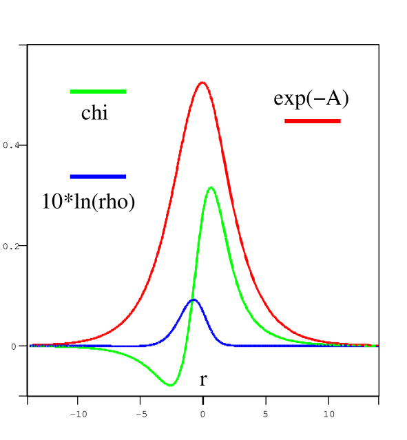
Figure 1: For small fermionic mass parameter $\chi_{0}$ the Euclidean wormhole solution (albeit non-perturbatively unstable) is singularity-free. A typical RG flow with $|\chi_{0}|<\chi_{singular}$. Here $\chi_{0}={\textstyle{\frac{1}{5}}}\chi_{critical}$.

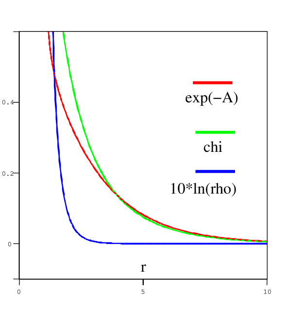
Figure 2: As we increase the fermionic mass parameter $|\chi_{0}|$, the Euclidean wormhole solution develops a naked singularity, before it can be stabilized against $D3\overline{D3}$ pair production. A typical RG flow with $\chi_{critical}>|\chi_{0}|>\chi_{singular}$. Here $\chi_{0}={\textstyle{\frac{1}{2}}}\chi_{critical}$.

In previous section we demonstrated that the wormhole (4.17) persists for small deformations, corresponding to turning on masses. From (4.16) small mass can’t cure the Schwinger-like instabilities of wormhole geometries due to the $D3\overline{D3}$ pair production. We would like to ask the question what happens with the wormhole solution once this instability is removed. To simplify the problem we will turn on only the fermionic masses, i.e., we set $\rho_{11}=\rho_{10}=\chi_{10}=0$. Inspection of RG flow equations shows that $\rho(r)$ is still a nontrivial function. This is just a reflection of the fact that bosonic masses are induced by higher loop effects, even though bare masses are set to zero. Without loss of generality we can choose the radial coordinate in such a way that $\xi=0$. Then (4.16) translates into

$$\chi_{0}^{2}>3\equiv\chi_{critical}^{2}\,.$$ (4.21)

Numerical integration of (4.7), with boundary data dependent only on $\chi_{0}$ as outlined above, reveals two different types of RG flows, separated by $\chi_{singular}$,

$$\frac{\chi_{singular}}{\chi_{critical}}\approx 0.3719\cdots\,.$$ (4.22)

For

$$|\chi_{0}|<\chi_{singular}\,,$$ (4.23)

the RG flow geometry is a smooth (albeit non-perturbatively unstable) wormhole. A typical behavior of the warp factor $A(r)$, and the 5d gauged supergravity scalars $\chi(r),\ \rho(r)$ is shown in Fig. 1.

As the fermionic mass parameter $|\chi_{0}|$ is increased above $\chi_{singular}$ (4.22), the background geometry develops a naked singularity. This singularity is associated with collapsing to zero size $\Sigma_{4}$, and correspondingly with the divergence of the stress-tensor of the supergravity scalars $\chi$ and $\rho$. A typical behavior of the RG flow in this regime is shown in Fig. 2. Since $\chi_{singular}<\chi_{critical}$, the Euclidean wormhole solution develops a naked singularity before it can be stabilized.

4.4 A comment on slow-role inflation in de-Sitter deformed ${\cal N}=2^{*}$ throats

One of the problems of brane inflation is generically large $\eta$ parameter (3.26), [22, 12]. We argue here that it appears to be possible to achieve slow-roll brane inflation in de-Sitter deformed ${\cal N}=2^{*}$ throats, $\Lambda>0$. Specifically, we demonstrate that $\eta$ can be made arbitrary small. Detailed study of this cosmological model will appear elsewhere [28].

Reintroducing $\Lambda$, (4.15) becomes

$$m_{\phi_{r}}^{2}=\frac{2}{3}\ \Lambda+\biggl{[}{\textstyle{\frac{2}{3}}}e^{2\xi}\chi_{0}^{2}\biggr{]}+\biggl{[}e^{2\xi}\rho_{11}\left({\textstyle{\frac{3}{2}}}\cos^{2}\theta-1\right)\biggr{]}\,,$$ (4.24)

thus leading to

$$\eta=\frac{2}{3}+\biggl{[}{\textstyle{\frac{2}{3}}}\Lambda^{-1}\ e^{2\xi}\chi_{0}^{2}\biggr{]}+\biggl{[}\Lambda^{-1}\ e^{2\xi}\rho_{11}\left({\textstyle{\frac{3}{2}}}\cos^{2}\theta-1\right)\biggr{]}\,.$$ (4.25)

We see that to reduce $\eta$, we, first of all, would like to turn off 3-form fluxes (fermionic mass parameter), i.e., set $\chi_{0}=0$. In fact, setting $\chi(r)\equiv 0$ is a consistent truncation of the full RG flow equations, (4.7). From (4.24), it is clear that a $D3$ probe would tend to move in the $\cos\theta=0$ ’valley’, where its potential energy is locally minimized. If we now identify the effective inflaton field with the radial motion of the $D3$ probe in the $\cos\theta=0$ valley, its $\eta$ parameter becomes

$$\eta=\frac{2}{3}-\Lambda^{-1}\ e^{2\xi}\rho_{11}\,,$$ (4.26)

which can be made arbitrary small by fine-tuning the deformation parameter $\rho_{11}$, corresponding to turning on masses to bosonic components of the ${\cal N}=2$ hypermultiplet, $m_{b}^{2}\sim\Lambda$. Given general arguments of [3], we expect such backgrounds to be singularity-free.

Appendix

Here we present ten-dimensional lift of five-dimensional RG flow of section 4.1. The 10d Einstein frame metric is

$$\begin{split}ds_{10}^{2}&=\Omega^{2}ds_{5}^{2}+4\frac{(cX_{1}X_{2})^{1/4}}{\rho^{3}}\biggl{(}c^{-1}d\theta^{2}+\rho^{6}\cos^{2}\theta\left(\frac{\sigma_{1}^{2}}{cX_{2}}+\frac{\sigma_{2}^{2}+\sigma_{3}^{2}}{X_{1}}\right)+\sin^{2}\theta\frac{d\phi^{2}}{X_{2}}\biggr{)}\,,\end{split}$$ (4.27)

where $ds_{5}^{2}$ is the five-dimensional flow metric (4.6), $c\equiv\cosh(2\chi)$. The warp factor is given by

$$\Omega^{2}=\frac{(cX_{1}X_{2})^{1/4}}{\rho}\,,$$ (4.28)

and the two functions $X_{i}$ are defined by

$$\begin{split}X_{1}(r,\theta)&=\cos^{2}\theta+\rho(r)^{6}\cosh(2\chi(r))\sin^{2}\theta\,,\\ X_{2}(r,\theta)&=\cosh(2\chi(r))\cos^{2}\theta+\rho(r)^{6}\sin^{2}\theta\,.\end{split}$$ (4.29)

Additionally, $\sigma_{i}$ are the $SU(2)$ left-invariant forms normalized so that $d\sigma_{i}=2\sigma_{j}\wedge\sigma_{k}$. For the dilaton/axion (compare with (3.4), (3.10)) we have

$$f=\frac{1}{2}\left(\left(\frac{cX_{1}}{X_{2}}\right)^{1/4}+\left(\frac{cX_{1}}{X_{2}}\right)^{-1/4}\right),\qquad f{\cal B}=\frac{1}{2}\left(\left(\frac{cX_{1}}{X_{2}}\right)^{1/4}-\left(\frac{cX_{1}}{X_{2}}\right)^{-1/4}\right)e^{2i\phi}\,.$$ (4.30)

The 3-form fluxes are

$$A_{(2)}=e^{i\phi}\left(a_{1}(r,\theta)\ d\theta\wedge\sigma_{1}+a_{2}(r,\theta)\ \sigma_{2}\wedge\sigma_{3}+a_{3}(r,\theta)\ \sigma_{1}\wedge d\phi+a_{4}(r,\theta)\ d\theta\wedge d\phi\right)\,,$$ (4.31)

where $a_{i}(r,\theta)$ are given by

$$\begin{split}a_{1}&=-i\ 4\ \tanh(2\chi)\cos\theta\,,\\ a_{2}&=i\ 4\ \frac{\rho^{6}\sinh(2\chi)}{X_{1}}\ \sin\theta\cos^{2}\theta\,,\\ a_{3}&=-4\ \frac{\sinh(2\chi)}{X_{2}}\ \sin\theta\cos^{2}\theta\,,\\ a_{4}&=0\,.\end{split}$$ (4.32)

Finally, the 5-form flux is

$$\begin{split}\qquad F_{5}={\cal F}+\star{\cal F}\,,\qquad{\cal F}={\rm vol}_{H^{4}}\wedge d\omega\,,\end{split}$$ (4.33)

where $\omega(r,\theta)$ satisfies

$$\begin{split}&\frac{\partial\omega}{\partial\theta}=-\frac{3}{2}e^{4A}\left(\ln\rho\right)^{\prime}\ \sin 2\theta\,,\\ &\frac{\partial\omega}{\partial r}=\frac{1}{8}e^{4A}\ \frac{1}{\rho^{4}}\ \biggl{(}-\rho^{12}\sinh^{2}(2\chi)\sin^{2}\theta+2\rho^{6}\cosh(2\chi)(1+\sin^{2}\theta)+2\cos^{2}\theta\biggr{)}\,.\end{split}$$ (4.34)

References

- [1] O. Aharony, S. S. Gubser, J. M. Maldacena, H. Ooguri and Y. Oz, “Large N field theories, string theory and gravity,” Phys. Rept. 323, 183 (2000) [arXiv:hep-th/9905111].
- [2] J. M. Maldacena, “The large N limit of superconformal field theories and supergravity,” Adv. Theor. Math. Phys. 2, 231 (1998) [Int. J. Theor. Phys. 38, 1113 (1999)] [arXiv:hep-th/9711200].
- [3] A. Buchel and A. A. Tseytlin, “Curved space resolution of singularity of fractional D3-branes on conifold,” Phys. Rev. D 65, 085019 (2002) [arXiv:hep-th/0111017].
- [4] A. Buchel, “Gauge / gravity correspondence in accelerating universe,” Phys. Rev. D 65, 125015 (2002) [arXiv:hep-th/0203041].
- [5] A. Buchel, P. Langfelder and J. Walcher, “On time-dependent backgrounds in supergravity and string theory,” Phys. Rev. D 67, 024011 (2003) [arXiv:hep-th/0207214].
- [6] A. Buchel, “Gauge / string correspondence in curved space,” Phys. Rev. D 67, 066004 (2003) [arXiv:hep-th/0211141].
- [7] A. Buchel, “Compactifications of the N = 2* flow,” Phys. Lett. B 570, 89 (2003) [arXiv:hep-th/0302107].
- [8] D. Bak, M. Gutperle and S. Hirano, “A dilatonic deformation of AdS(5) and its field theory dual,” JHEP 0305, 072 (2003) [arXiv:hep-th/0304129].
- [9] J. Maldacena and L. Maoz, “Wormholes in AdS,” arXiv:hep-th/0401024.
- [10] N. Seiberg and E. Witten, “The D1/D5 system and singular CFT,” JHEP 9904, 017 (1999) [arXiv:hep-th/9903224].
- [11] I. R. Klebanov and M. J. Strassler, “Supergravity and a confining gauge theory: Duality cascades and chiSB-resolution of naked singularities,” JHEP 0008, 052 (2000) [arXiv:hep-th/0007191].
- [12] A. Buchel and R. Roiban, “Inflation in warped geometries,” arXiv:hep-th/0311154.
- [13] R. Emparan, “AdS/CFT duals of topological black holes and the entropy of zero-energy states,” JHEP 9906, 036 (1999) [arXiv:hep-th/9906040].
- [14] S. S. Gubser and I. Mitra, “Instability of charged black holes in anti-de Sitter space,” arXiv:hep-th/0009126.
- [15] H. Van Hees and J. Knoll, “Renormalization of self-consistent approximation schemes. II: Applications to the sunset diagram,” Phys. Rev. D 65, 105005 (2002) [arXiv:hep-ph/0111193].
- [16] J. H. Schwarz, “Covariant Field Equations of Chiral Supergravity,” Nucl. Phys. B226 (1983) 269.
- [17] S. B. Giddings, S. Kachru and J. Polchinski, “Hierarchies from fluxes in string compactifications,” Phys. Rev. D 66, 106006 (2002) [arXiv:hep-th/0105097].
- [18] A. Buchel, “On effective action of string theory flux compactifications,” to appear in Phys. Rev. D, arXiv:hep-th/0312076.
- [19] J. Polchinski, “String Theory. Vol. 2: Superstring Theory And Beyond,”
- [20] L. Randall and R. Sundrum, “An alternative to compactification,” Phys. Rev. Lett. 83, 4690 (1999) [arXiv:hep-th/9906064].
- [21] S. Kachru, R. Kallosh, A. Linde and S. P. Trivedi, “De Sitter vacua in string theory,” Phys. Rev. D 68, 046005 (2003) [arXiv:hep-th/0301240].
- [22] S. Kachru, R. Kallosh, A. Linde, J. Maldacena, L. McAllister and S. P. Trivedi, “Towards inflation in string theory,” JCAP 0310, 013 (2003) [arXiv:hep-th/0308055].
- [23] I. R. Klebanov and A. A. Tseytlin, “Gravity duals of supersymmetric SU(N) x SU(N+M) gauge theories,” Nucl. Phys. B 578, 123 (2000) [arXiv:hep-th/0002159].
- [24] K. Pilch and N. P. Warner, “N = 2 supersymmetric RG flows and the IIB dilaton,” Nucl. Phys. B 594, 209 (2001) [arXiv:hep-th/0004063].
- [25] A. Buchel, A. W. Peet and J. Polchinski, “Gauge dual and noncommutative extension of an N = 2 supergravity solution,” Phys. Rev. D 63, 044009 (2001) [arXiv:hep-th/0008076].
- [26] N. Evans, C. V. Johnson and M. Petrini, “The enhancon and N = 2 gauge theory/gravity RG flows,” JHEP 0010, 022 (2000) [arXiv:hep-th/0008081].
- [27] A. Buchel and J. T. Liu, “Thermodynamics of the N = 2* flow,” JHEP 0311, 031 (2003) [arXiv:hep-th/0305064].
- [28] A. Buchel and A. Ghodsi, “Braneworld inflation,” arXiv:hep-th/0404151.