Concerning the generalized Lorentz symmetry and the generalization of the Dirac equation

G.Yu. Bogoslovsky ${}^{a,\,}$,  H.F. Goenner ${}^{b,\,}$
^a Skobeltsyn Institute of Nuclear Physics, Moscow State University
119992 Moscow, Russia
^b Institute for Theoretical Physics, University of Göttingen, 37081 Göttingen, Germany

  Abstract The work is devoted to the generalization of the Dirac equation for a flat locally anisotropic, i.e., Finslerian space-time. At first we reproduce the corresponding metric and a group of the generalized Lorentz transformations, which has the meaning of the relativistic symmetry group of such event space. Next, proceeding from the requirement of the generalized Lorentz invariance we find a generalized Dirac equation in its explicit form. An exact solution of the nonlinear generalized Dirac equation is also presented.
PACS :  03.30.+p; 03.65.Pm; 11.30.Cp; 11.30.Qc; 02.20.Sv; 02.40.Hw
Keywords : Finslerian space-time; Dirac equations; Lorentz, Poincaré and gauge invariance;
Keywords : Spontaneous symmetry breaking

 

In spite of the impressive successes of the unified gauge theory of strong, weak and electromagnetic interactions, known as the Standard Model, one cannot a priori rule out the possibility that Lorentz symmetry underlying the theory is an approximate symmetry of nature. This implies that at the energies already attainable today empirical evidence may be obtained in favour of violation of Lorentz symmetry. At the same time it is obvious that such effects might manifest themselves only as strongly suppressed effects of Planck-scale physics.

Theoretical speculations about a possible violation of Lorentz symmetry continue for more than forty years and they are briefly outlined in [1]. Nevertheless we note here that, along with the spontaneous breaking [2], one of the first and, as it appeared subsequently, fruitful ideas relating to a possible violation of Lorentz symmetry was the idea [3] according to which the metric of event space differs from Minkowski metric and the physically equivalent inertial reference frames are linked by some transformations which differ from Lorentz ones. In [4] such transformations were called generalized Lorentz transformations. Note also that the idea about the existence of generalized Lorentz transformations was suggested in connection with the situation in the physics of ultra-high energy cosmic rays, namely, with the absence of the Greisen-Zatsepin-Kuz’min effect (the so-called GZK cutoff) predicted [5, 6] on the basis of conventional relativistic theory. The absence of the GZK cutoff has yet not been explained convincingly and still remains the main empirical fact which indirectly speaks in favour of violation of Lorentz symmetry.

Interest in the problem of violation of Lorentz and CPT symmetries has revived in recent years [7] in connection with the construction of a phenomenological theory reffered to as the Standard-Model Extension [8].

In the present work, which is in essence devoted to the same problem, we proceed from the assumption [9] that phase transitions with breaking of gauge symmetries should be accompanied by phase transitions in the geometric structure of space-time.

Our study is based on the fact [10] that the Lorentz symmetry is not the only possible realization of the relativistic symmetry. Another admissible realization of the relativistic symmetry is obtained with the aid of nonunimodular matrices belonging to a group of the generalized Lorentz transformations. In contrast to the conventional Lorentz transformations, the generalized ones conformally modify Minkowski metric but leave invariant the corresponding Finslerian metric which describes a flat locally anisotropic space-time. Thus, from the formal point of view the locally anisotropic space-time appeares as the necessary consequence of the existence of a group of the generalized Lorentz transformations. As for the physical nature of the anisotropy, there are some reasons to suppose that a fermion-antifermion condensate, which may arise [11] (instead of elementary Higgs condensate) in the spontaneous breaking of initial gauge symmetries, turns out to be anisotropic and its anisotropy determines the local anisotropy of event space. Obviously, verification of this hypothesis is far from being trivial. Therefore the opening investigations in this direction, as presented here, are aimed at the most fundamental problem, namely, at the generalization of the Dirac equation for the locally anisotropic space-time.

Consider the metric [4] of a flat locally anisotropic space-time

$$ds^{2}=\left[\frac{(dx_{0}-\boldsymbol{\nu}d\boldsymbol{x})^{2}}{dx_{0}^{2}-d\boldsymbol{x}^{\,2}}\right]^{r}(dx_{0}^{2}-d\boldsymbol{x}^{\,2})\,.$$ (1)

Being not a quadratic form but a homogeneous function of the coordinate differentials of degree two, this metric falls within the category of Finsler metrics [12]. It depends on two constant parameters $r$ and $\boldsymbol{\nu}$, in which case the unit vector $\boldsymbol{\nu}$ indicates a preferred direction in 3D space while $r$ determines the magnitude of space anisotropy, characterizing the degree of deviation of the metric (1) from the Minkowski metric. Thus the anisotropic event space (1) is the generalization of the isotropic Minkowski space of conventional special relativity theory.

The 3-parameter noncompact group of the generalized Lorentz transformations, which leave the metric (1) invariant, appears as

$$x^{\prime}\,{}^{i}=D(\boldsymbol{v},\boldsymbol{\nu})\,R^{i}_{j}(\boldsymbol{v},\boldsymbol{\nu})\,L^{j}_{k}(\boldsymbol{v})\,x^{k}\,,$$ (2)

where $\boldsymbol{v}$ denotes the velocities of moving (primed) inertial reference frames; the matrices $\,L^{j}_{k}(\boldsymbol{v})\,$ represent the ordinary Lorentz boosts; the matrices $\,R^{i}_{j}(\boldsymbol{v},\boldsymbol{\nu})\,$ represent additional rotations of the spatial axes of the moving frames around the vectors $\,[\boldsymbol{v}\,\boldsymbol{\nu}]\,$ through the angles

$$\varphi=\arccos\left\{1-\frac{(1-\sqrt{1-\boldsymbol{v}^{\,2}/c^{2}})[\boldsymbol{v}\boldsymbol{\nu}]^{2}}{(1-\boldsymbol{v}\boldsymbol{\nu}/c)\boldsymbol{v}^{\,2}}\right\}$$

of relativistic aberration of $\boldsymbol{\nu}\,;$ and the diagonal matrices

$$D(\boldsymbol{v},\boldsymbol{\nu})=\left(\frac{1-\boldsymbol{v}\boldsymbol{\nu}/c}{\sqrt{1-\boldsymbol{v}^{\,2}/c^{2}}}\right)^{r}I\,,$$

the additional dilatational transformations of the event coordinates. The structure of the transformations (2) ensures the fact that in spite of a new geometry of event space the 3-velocity space remains Lobachevski space.

With the inclusion of the 1-parameter group of rotations about $\,\boldsymbol{\nu}\,$ and of the 4-parameter group of translations the inhomogeneous isometry group of the Finslerian event space (1) turns out to have eight parameters. If the third spatial axis is chosen along $\,\boldsymbol{\nu}\,,$ then its generators can be written as

$$\begin{array}[]{rcl}X_{1}&=&-(x^{1}p_{0}+x^{0}p_{1})-(x^{1}p_{3}-x^{3}p_{1})\,,\\ X_{2}&=&-(x^{2}p_{0}+x^{0}p_{2})+(x^{3}p_{2}-x^{2}p_{3})\,,\\ X_{3}&=&-rx^{i}p_{i}-(x^{3}p_{0}+x^{0}p_{3})\,,\\ R_{3}&=&x^{2}p_{1}-x^{1}p_{2}\,;\qquad\qquad\qquad\qquad\qquad p_{i}=\partial/\partial x^{i}\,.\\ \end{array}$$

These generators satisfy the commutation relations

$$\begin{array}[]{llll}[X_{1}X_{2}]=0\,,&[R_{3}X_{3}]=0\,,&&\\ \left[X_{3}X_{1}\right]=X_{1}\,,&[R_{3}X_{1}]=X_{2}\,,&&\\ \left[X_{3}X_{2}\right]=X_{2}\,,&[R_{3}X_{2}]=-X_{1}\,;&&\\ \left[p_{i}p_{j}\right]=0\,;&&&\\ \left[X_{1}p_{0}\right]=p_{1}\,,&[X_{2}p_{0}]=p_{2}\,,&[X_{3}p_{0}]=rp_{0}+p_{3}\,,&[R_{3}p_{0}]=0\,,\\ \left[X_{1}p_{1}\right]=p_{0}+p_{3}\,,&[X_{2}p_{1}]=0\,,&[X_{3}p_{1}]=rp_{1}\,,&[R_{3}p_{1}]=p_{2}\,,\\ \left[X_{1}p_{2}\right]=0\,,&[X_{2}p_{2}]=p_{0}+p_{3}\,,&[X_{3}p_{2}]=rp_{2}\,,&[R_{3}p_{2}]=-p_{1}\,,\\ \left[X_{1}p_{3}\right]=-p_{1}\,,&[X_{2}p_{3}]=-p_{2}\,,&[X_{3}p_{3}]=rp_{3}+p_{0}\,,&[R_{3}p_{3}]=0\,.\\ \end{array}$$

As one can see the 8-parameter inhomogeneous isometry group of the space-time (1) is a subgroup of the 11-parameter extended Poincaré (similitude) group [13] whereas the homogeneous one is isomorphic to the corresponding 4-parameter subgroup (with the generators $X_{1}\,,X_{2}\,,X_{3}\!\!\mid_{r=0}\,,R_{3}$) of the homogeneous Lorentz group. It is shown in [14] that the 6-parameter homogeneous Lorentz group has no 5-parameter subgroup while the 4-parameter subgroup is unique (up to isomorphisms). Thus, the transition from Minkowski space to the Finslerian event space (1) implies a minimum of symmetry-breaking of the Lorentz symmetry. However the relativistic symmetry is maintained in the form of the generalized Lorentz symmetry.

Because of nonunimodularity of the matrices ${\cal L}^{i}_{k}=DR^{i}_{j}L^{j}_{k}$ representing the generalized Lorentz transformations (2), the transformational properties of some geometric entities turn out to be changed as compared with conventional special relativity theory. For instance, a 4-volume element $dx^{0}d^{3}x$ is no longer invariant but is a scalar density of weight $-1\,,$ i.e., it transforms as follows: $\,dx^{\prime}{}^{0}d^{3}x^{\prime}=J^{-1}dx^{0}d^{3}x\,,$ where $J$ is the Jacobian, $\,J=|\partial x^{k}/\partial x^{\prime}{}^{j}|=|{{\cal L}^{-1}}^{k}_{j}|=D^{-4}\,.$ Similarly, matrices $\,{\eta}_{i}{}_{k}\,$ and $\,{\eta}^{i}{}^{k}\,$ having the identical forms $\,{\eta}_{i}{}_{k}=diag\,(1,-1,-1,-1)\,$ and $\,{\eta}^{i}{}^{k}=diag\,(1,-1,-1,-1)\,$ in all frames of reference related by the transformations (2) are no longer invariant tensors but are, respectively, a covariant tensor density of weight $-1/2$ and a contravariant tensor density of weight $1/2.$ This statement signifies that $\,{{\eta}^{\prime}}_{i}{}_{k}=J^{-1/2}{{\cal L}^{-1}}^{l}_{i}{{\cal L}^{-1}}^{m}_{k}{\eta}_{l}{}_{m}={\eta}_{i}{}_{k}\,$ and $\,{{\eta}^{\prime}}^{i}{}^{k}=J^{1/2}{\cal L}^{i}_{l}{\cal L}^{k}_{m}{\eta}^{l}{}^{m}={\eta}^{i}{}^{k}\,.$ Then it is clear that $\,{\eta}_{i}{}_{k}{\eta}^{k}{}^{l}={\delta}^{l}_{i}\,$ is a unit tensor. Later on we shall be using $\,{\eta}_{i}{}_{k}\,$ and $\,{\eta}^{i}{}^{k}\,$ to lower and raise indices. The process, however, will be accompanied by a change in weight. We shall be also in need of an entity $\,{\nu}^{i}\,$ which indicates a preferred direction in 4D space-time and whose components have the same values, $\,\left\{\,{\nu}^{0}=1\,,\,\boldsymbol{\nu}\,\right\}\,,$ in all frames of reference related by the transformations (2). It is easy to verify that $\,{\nu}^{\prime}{}^{i}=J^{(1+r)/(4r)}{\cal L}^{i}_{k}{\nu}^{k}={\nu}^{i}\,,$ i.e., that $\,{\nu}^{i}\,$ is a contravariant vector density of weight $\,(1+r)/(4r)\,,$ in which case $\,{\nu}_{i}{\nu}^{i}=0\,$ is an invariant equation.

Using the $\,{\nu}^{i}\,$ and $\,{\eta}_{i}{}_{k}\,$ one can represent the metric (1) as an explicit invariant of the transformations (2) : $\,ds^{2}=\left[({\nu}_{i}dx^{i})^{2}/dx_{j}dx^{j}\right]^{r}dx_{k}dx^{k}\,.$ With the aid of this expression we arrive at the relativistically invariant action for a free particle in the flat anisotropic space. The action and its variation appear as

$$S=-m\int\limits_{a}^{b}ds\,,\quad\delta S=-\int\limits_{a}^{b}p_{i}\,d\,\delta x^{i}\,.$$

Hereafter we put $\,c=\hbar=1\,.$ The principle of least action under the condition $\,(\delta x^{i})\,|_{a}=(\delta x^{i})\,|_{b}=0\,$ leads to $\,p_{i}=const,$ i.e., to rectilinear inertial motion. And if one varies the coordinates of point $b$ under the condition $\,p_{i}=const\,,$ then $\,p_{i}=-\partial S/\partial x^{i}\,,$ i.e., $\,p_{i}\,$ is a canonical 4-momentum. Since $\,{\eta}^{i}{}^{k}\,$ is a contravariant tensor density of weight $1/2$ and since $\,p_{k}\,$ is a covariant vector it is clear that the 4-momentum $\,p^{i}=(p^{0},\,\boldsymbol{p})={\eta}^{i}{}^{k}p_{k}\,$ is transformed as a contravariant vector density of $1/2,$ i.e.,

$${p^{\prime}}^{\,i}=J^{1/2}{\cal L}^{i}_{k}\,p^{k}=D^{-1}R^{i}_{l}L^{l}_{k}\,p^{k}\,.$$ (3)

Thus we have arrived at the generalized Lorentz transformations for 4-momenta. Note that the dilatational transformations of $\,p^{i}\,$ are inverse to those of $\,x^{i}\,$ ( cf. (2) ) . In an explicit form

$$p^{i}=m\left(\frac{\nu_{l}dx^{l}}{\sqrt{dx_{j}dx^{j}}}\right)^{r}\left((1-r)\frac{dx^{i}}{\sqrt{dx_{a}dx^{a}}}+r\frac{\nu^{i}\sqrt{dx_{b}dx^{b}}}{\nu_{n}dx^{n}}\right)\,.$$ (4)

Since the direction of $\,p^{i}\,$ is not aligned with the direction of $\,dx^{i}\,$ we introduce (apart from $\,p^{i}\,$) the so-called kinematic 4-momentum $\,k^{i}\,$ which has the same transformational properties as $\,p^{i}\,.$

$$k^{i}=m\,(1-r)\frac{dx^{i}}{\sqrt{dx_{n}dx^{n}}}\left(\frac{\nu_{l}dx^{l}}{\sqrt{dx_{j}dx^{j}}}\right)^{r}\,.$$ (5)

Taking into account the equation $\,{\nu}_{i}{\nu}^{i}=0\,$ we obtain the following relations

$$p^{i}=k^{i}+\frac{r\,k_{l}k^{l}}{(1-r)k_{n}\nu^{n}}\,\nu^{i}\,,\qquad k^{i}=p^{i}-\frac{r\,p_{l}p^{l}}{(1+r)p_{n}\nu^{n}}\,\nu^{i}\,.$$ (6)

As for the 3-velocity of a particle, it is determined by the formula $\,\boldsymbol{v}=\boldsymbol{k}/k^{0}\,$. The components of canonical 4-momenta satisfy the mass shell equation

$$\left[({\nu}_{i}p^{i})^{2}/p_{j}p^{j}\right]^{-r}p_{a}p^{a}=m^{2}(1-r)^{(1-r)}(1+r)^{(1+r)}\,.$$ (7)

This equation is an invariant of the transformations (3). The same mass shell but in a space of kinematic 4-momenta is described by the equation

$$\left[({\nu}_{i}k^{i})^{2}/k_{j}k^{j}\right]^{-r}k_{a}k^{a}=m^{2}(1-r)^{2}\,.$$ (8)

The last two equations lead us to the important conclusion, namely, that the motion of free massless particles in anisotropic space is similar to their motion in isotropic space, i.e., massless particles do not perceive the space anisotropy whereas the motion of massive particles is analogous to that of quasiparticles in a crystalline medium.

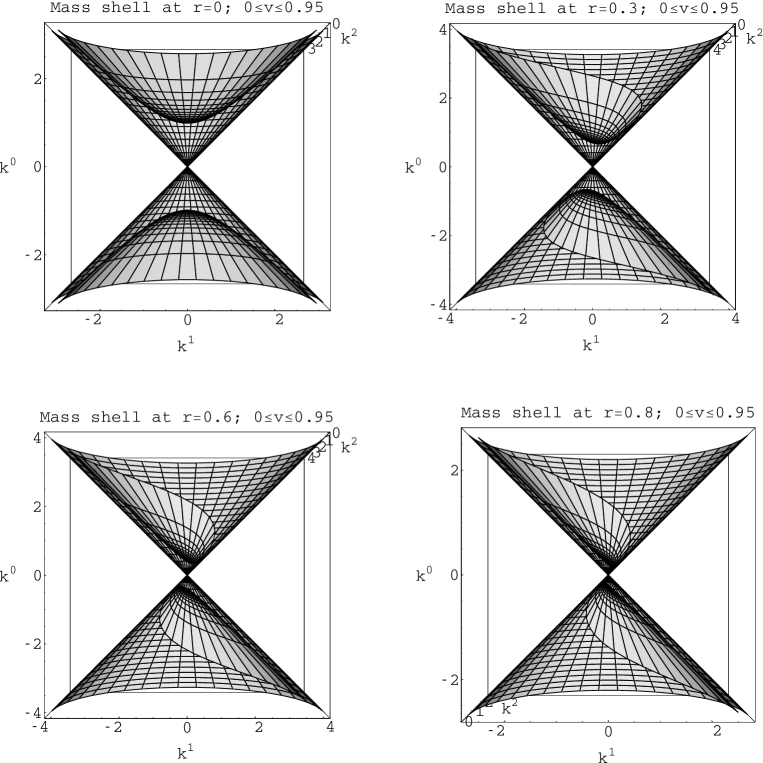
Figure 1: Parametric 3D plots of the mass shells in a space of kinematic 4-momenta.

According to (8), the mass shell for $\,r\neq 0\,$ is a deformed two-sheeted hyperboloid inscribed into a light cone. In order to show how its deformation changes with the magnitude $\,r\,$ of space anisotropy it is reasonable to proceed from the relations (5) which determine four-dimensional coordinates of points belonging to the upper sheet of the deformed hyperboloid as explicit functions of 3-velocities $\,\boldsymbol{v}=d\boldsymbol{x}/dx^{0}\,.$ The results of calculations, presented in Fig. 1 clearly demonstrate the fact that, if $\,r\to 1\,,$ the mass shell in a space of kinematic 4-momenta converges (nonuniformly) to a light cone. As for the canonical momenta $\,p^{i}\,,$ there is nonuniform convergence : $\,p^{i}\to k^{i}+m{\nu}^{i}\,,$ where $\,k_{i}k^{i}=0\,.$ Physically this means that the effective inertial mass of a particle present in anisotropic (Finslerian) space depends on the magnitude $\,r\,$ of a constant anisotropy field and disappears at all if $\,r\,$ reaches the value equal to unity.

Thus, with a view to generalizing the Dirac Lagrangian for the Finslerian space-time (1), we have arrived at the following guiding principle : a generalized Lagrangian, in the limit $\,r=1\,,$ must be reducible (up to a 4-divergence) to the standard massless Dirac Lagrangian.

Starting to generalize the Dirac Lagrangian, first consider the standard massless one $\,(i/2)\left(\bar{\psi}{\gamma}^{n}{\partial}_{n}\psi-{\partial}_{n}\bar{\psi}{\gamma}^{n}\psi\right)\,.$ Since massless particles do not perceive the space anisotropy, the Lagrangian considered need not be modified and it can be used as the kinetic term of a massive generalized Dirac Lagrangian. Since under the generalized Lorentz transformations (2) the 4-volume $\,dx^{0}d^{3}x\,$ behaves as a scalar density of weight $\,-1\,$ and the action must remain invariant, it follows that the kinetic term ( just as the entire Lagrangian ) must be a scalar density of weight $\,1\,.$ This condition is fulfilled in the case where the generalized Lorentz transformations (2) of the coordinates are accompanied by the following transformations of the fields $\,\psi\,$ and $\,\bar{\psi}\,:$

$$\psi^{\prime}(x^{\prime})=D^{-3/2}S_{R}S_{L}\psi(x)=J^{3/8}S\psi(x)\,,$$ (9)

$$\bar{\psi}^{\prime}(x^{\prime})=\bar{\psi}(x)J^{3/8}S^{-1}\,,$$ (10)

where the matrices $\,S=S_{R}S_{L}\,$ satisfy the standard condition $\,S^{-1}\gamma^{i}S=\Lambda^{i}_{k}\gamma^{k}\,,$ in which case $\,\Lambda^{i}_{k}=R^{i}_{j}L^{j}_{k}\,;$ the matrices $\,S_{L}\,$ and $\,S_{R}\,$ represent, respectively, the Lorenz boosts and additional rotations of bispinors. In an explicit form

$$S_{L}=\sqrt{\frac{1\!+\!\sqrt{1\!-\!{\boldsymbol{v}}^{2}}}{2\sqrt{1\!-\!{\boldsymbol{v}}^{2}}}}\,I-\sqrt{\frac{1\!-\!\sqrt{1\!-\!{\boldsymbol{v}}^{2}}}{2\sqrt{1\!-\!{\boldsymbol{v}}^{2}}}}\,\,\frac{{\gamma}^{0}\boldsymbol{v}\boldsymbol{\gamma}}{|\boldsymbol{v}|}\,,$$ (11)

$$S_{R}=\sqrt{1\!-\!\frac{(1\!-\!\sqrt{1\!-\!{\boldsymbol{v}}^{2}})[\boldsymbol{v}\boldsymbol{\nu}]^{2}}{2(1\!-\!\boldsymbol{v}\boldsymbol{\nu})\,{\boldsymbol{v}}^{2}}}\,I+i\sqrt{\frac{1\!-\!\sqrt{1\!-\!{\boldsymbol{v}}^{2}}}{2(1\!-\!\boldsymbol{v}\boldsymbol{\nu})}}\,\frac{[\boldsymbol{v}\boldsymbol{\nu}]}{|\boldsymbol{v}|}\,\boldsymbol{\Sigma}\,,$$ (12)

where $\,\boldsymbol{v}\,$ denotes the velocities of moving (primed) reference frames, $\,{\gamma}^{n}\,$ are the Dirac matrices, $\,\boldsymbol{\Sigma}=diag\,(\,\boldsymbol{\sigma}\,,\boldsymbol{\sigma}\,)\,$ and $\,\boldsymbol{\sigma}\,$ are the Pauli matrices. Thus in the flat Finslerian space-time (1) the fields $\,\psi\,$ and $\,\bar{\psi}\,$ are, according to (9) and (10), bispinor density fields of weight $\,3/8\,.$

In order to generalize the massive term $\,-m\bar{\psi}\psi\,$ of the Dirac Lagrangian we remind that a generalized massive term, like the kinetic one, must be a scalar density of weight $1\,.$ It can be verified that for the bispinor density fields : $\,\bar{\psi}\psi\,$ is a scalar density of weight $\,3/4\,,$ $\,\,\bar{\psi}{\gamma}^{n}\psi\,$ is a contravariant vector density of weight $1\,,$ $\,[({\nu_{n}\bar{\psi}\gamma^{n}\psi}/{\bar{\psi}\psi})^{2}]^{r/2}\bar{\psi}\psi\,$ is a scalar density of weight $\,1\,$ and $\,[({\nu_{n}\bar{\psi}\gamma^{n}\psi}/{\bar{\psi}\psi})^{2}]^{-3r/2}\bar{\psi}\psi\,$ is a scalar, in which case the latter Finslerian form generalizes the scalar bilinear form $\,\bar{\psi}\psi\,$ of conventional theory.

Now we are able to write down a Lagrangian for the bispinor density fields representing such a generalization of the standard Dirac Lagrangian that the corresponding field equations turn out to be invariant under the group of generalized Lorentz transformations. It appears as

$${\cal L}=\frac{i}{2}\left(\bar{\psi}{\gamma}^{n}{\partial}_{n}\psi-{\partial}_{n}\bar{\psi}{\gamma}^{n}\psi\right)-m\!\left[\!\left(\frac{\nu_{n}\bar{\psi}\gamma^{n}\psi}{\bar{\psi}\psi}\right)^{\!\!\!2}\right]^{\!r/2}\!\!\bar{\psi}\psi\,.$$

This Lagrangian leads to the following generalized Dirac equations :

$$i\gamma^{a}{\partial}_{a}\psi\!-\!m\!\!\left[\!\left(\frac{\nu_{n}j^{n}}{\bar{\psi}\psi}\right)^{\!\!\!2}\right]^{\!\frac{r}{2}}\!\!\!\left\{\!\!(1\!-\!r)I\!+\!r\!\left(\frac{\bar{\psi}\psi}{\nu_{n}j^{n}}\right)\!\nu_{a}\gamma^{a}\!\right\}\!\psi=0\,,$$ (13)

$$i{\partial}_{a}\bar{\psi}\gamma^{a}\!+\!m\!\!\left[\!\left(\frac{\nu_{n}j^{n}}{\bar{\psi}\psi}\right)^{\!\!\!2}\right]^{\!\frac{r}{2}}\!\!\bar{\psi}\!\left\{\!\!(1\!-\!r)I\!+\!r\!\left(\frac{\bar{\psi}\psi}{\nu_{n}j^{n}}\right)\!\nu_{a}\gamma^{a}\!\right\}=0\,,$$ (14)

where $\,j^{n}=\bar{\psi}{\gamma}^{n}\psi\,.$ The operation : $\,\bar{\psi}$ (13) + (14) $\psi\,$ provides the equation $\,\partial_{n}j^{n}=0\,.$ Thus $\,j^{n}\,$ is a preserved current. And at last, owing to the operation : $\,\bar{\psi}$ (13) – (14) $\psi\,,$ we conclude that $\,{\cal L}=0\,$ on the solutions of eqs. (13) and (14).

Due to translational invariance, the generalized Dirac equations (13), (14) must admit solutions in the form of plane waves $\,\psi(x)=u(p)\exp{(-ip_{a}x^{a})}\,.$ This means that the amplitude $\,u(p)\,$ must satisfy the equations :

$$p_{a}\!\left[\gamma^{a}\!-\!\left(\frac{\bar{u}\gamma^{a}u}{\bar{u}u}\right)\!\!\left\{\!(1\!-\!r)I\!+\!r\!\left(\frac{\bar{u}u}{\nu_{l}\bar{u}\gamma^{l}u}\right)\nu_{n}\gamma^{n}\right\}\right]\!u=0\,,$$ (15)

$$\bar{u}p_{a}\!\left[\gamma^{a}\!-\!\left(\frac{\bar{u}\gamma^{a}u}{\bar{u}u}\right)\!\!\left\{\!(1\!-\!r)I\!+\!r\!\left(\frac{\bar{u}u}{\nu_{l}\bar{u}\gamma^{l}u}\right)\nu_{n}\gamma^{n}\right\}\right]=0\,,$$ (16)

$$p_{a}\bar{u}\gamma^{a}u=m\left[\!\left(\frac{\nu_{l}\bar{u}\gamma^{l}u}{\bar{u}u}\right)^{\!\!\!2}\right]^{\!r/2}\!\!\bar{u}u\,.$$ (17)

Eqs. (15)–(17) lead to the invariant dispersion relation

$$\sqrt{p_{a}p^{a}/(1-r^{2})}=\pm\,m\left[(1+r)({\nu}_{i}p^{i})^{2}/((1-r)p_{j}p^{j})\right]^{r/2}\,,$$ (18)

where the sign$\,+$ corresponds to positive frequency states whereas the sign$\,-$ corresponds to negative ones. It is worth mentioning that the mass shell equation (7) can be obtained from (18). In order to find the planewave solutions in a general form, i.​ e., at arbitrary momentum ​$p^{a}$ we, for a start, confine ourselves to the rest frame and try the following ansatz :

$${\psi}_{+}(x)=\sqrt{2m(1\!-\!r)}\left(\begin{array}[]{cc}\varphi\\ 0\end{array}\right)e^{-i(mx^{0}-mr\boldsymbol{\nu}\boldsymbol{x})}\quad,$$

$${\psi}_{-}(x)=\sqrt{2m(1\!-\!r)}\left(\begin{array}[]{cc}0\\ \chi\end{array}\right)e^{i(mx^{0}-mr\boldsymbol{\nu}\boldsymbol{x})}\quad,$$

where $\,\sqrt{2m(1\!-\!r)}\,$ is a normalizing multiplier and $\,\varphi\,,\,\chi\,$ are arbitrary 3-spinors normalized by means of $\,{\varphi}^{\dagger}\varphi=1\,,\,{\chi}^{\dagger}\chi=1\,.$ It is easy to verify that the corresponding positive and negative frequency bispinor density amplitudes satisfy Eqs. (15)–(17). Note once more that these solutions are found in the rest frame, in which $\,p^{a}=\{m\,,rm\boldsymbol{\nu}\}\,,$ whereas kinematic 4-momentum $\,k^{a}=\{m(1-r)\,,\boldsymbol{0}\}\,$ and, respectively, $\,\boldsymbol{v}=\boldsymbol{k}/k^{0}=0\,.$ Taking into account the transformational properties (9)–(12) we find planewave solutions of Eq.(13) in the final form :

$${\psi}_{+}(x)=\frac{\sqrt{k_{0}^{2}\!-\!{\boldsymbol{k}}^{2}}}{m(1\!-\!r)}\left(\!\begin{array}[]{lll}\!\sqrt{k_{0}\!+\!\sqrt{k_{0}^{2}\!-\!{\boldsymbol{k}}^{2}}}\,\,\,\varphi\\ \phantom{a}\\ \sqrt{k_{0}\!-\!\sqrt{k_{0}^{2}\!-\!{\boldsymbol{k}}^{2}}}\,\,\,(\boldsymbol{n}\boldsymbol{\sigma})\varphi\end{array}\!\right)e^{-i\,p_{a}\,x^{a}}\,,$$

$${\psi}_{-}(x)=\frac{\sqrt{k_{0}^{2}\!-\!{\boldsymbol{k}}^{2}}}{m(1\!-\!r)}\left(\!\begin{array}[]{lll}\!\sqrt{k_{0}\!-\!\sqrt{k_{0}^{2}\!-\!{\boldsymbol{k}}^{2}}}\,\,\,(\boldsymbol{n}\boldsymbol{\sigma})\chi\\ \phantom{a}\\ \sqrt{k_{0}\!+\!\sqrt{k_{0}^{2}\!-\!{\boldsymbol{k}}^{2}}}\,\,\,\chi\end{array}\!\right)e^{i\,p_{a}\,x^{a}}\,,$$

where the unit vector $\,\boldsymbol{n}\,$ indicates the direction of $\,\boldsymbol{k}\,,$ in which case $\,k^{a}\,$ and $\,p^{a}\,$ are related by (6). The bispinor density fields $\,\,{\psi}_{\pm}\,\,$ are normalized with the help of the invariant conditions  : $\,[({\nu_{n}{\bar{\psi}}_{\pm}\gamma^{n}{\psi}_{\pm}}/{{\bar{\psi}}_{\pm}{\psi}_{\pm}})^{2}]^{-3r/2}{\bar{\psi}}_{\pm}{\psi}_{\pm}=\pm\,2m(1\!-\!r)\,.$ As for the dispersion relation (18), in terms of $\,k^{a}\,$ it takes the form $\,\sqrt{k_{a}k^{a}}=\pm\,m(1-r)\left[({\nu}_{i}k^{i})^{2}/k_{j}k^{j}\right]^{r/2}\,.$ One of its solutions corresponds to massive fermions and, according to (5), admits the parametric representation by means of 3-velocities $\,\boldsymbol{v}\,.$ Another solution corresponds to massless fermions and has the form $\,k^{a}\propto{\nu}^{a}\,.$ Note at last that, in the limit $r=1,$ Eq. (13) takes the form $\,i\gamma^{a}{\partial}_{a}\psi\!-\!m{\nu}_{a}{\gamma}^{a}\psi=0\,$ and, after the local gauge transformation $\,\psi\to exp{(-im{\nu}_{a}x^{a})}\,\psi\,\,,$ reduces to the massless Dirac equation.

Summing up the results of the present work, we would like to emphasize that the spontaneous breaking of Lorentz symmetry does not necessarily signify the breaking of relativistic symmetry and may turn out to be a secondary effect induced by the spontaneous breaking of gauge symmetry. Here, the 10-parameter Poincaré group of an initial massless gauge-invariant theory is reduced to the 8-parameter inhomogeneous group of the generalized Lorentz transformations, which assumes in this case the role of the relativistic symmetry group of the corresponding vacuum solution of the theory. And vacuum itself, if it is regarded as space-time filled with a fermion-antifermion condensate, assumes anisotropic Finslerian geometry instead of Minkowski geometry. Within the framework of this picture the rearrangement of initial vacuum and the appearance of masses in the initial massless fields are not due to the standard Higgs mechanism but result from collective quantum effects peculiar to nonlinear dynamic systems.

Reverting to the translationally invariant generalized Dirac equation (13), which was obtained from the requirement of the generalized Lorentz symmetry, we see that it is essentially nonlinear. However this nonlinearity disappears in two cases : firstly, if the anisotropy field, constant over the whole space ( and more exactly, its magnitude $r\,$) tends to zero ( in this case (13) changes to the standard massive Dirac equation ), and secondly, if $\,r\,$ tends to its maximally attainable value equal to unity. In the latter case the anisotropy field turns out to be purely gauge while the massive fermion-antifermion field proves itself as the corresponding massless one. This means that the equation (13) describes the dynamics of the massive fermion-antifermion field in an anisotropic medium (in a relativistically invariant anisotropic condensate), in which case the effective inertial mass of the fermion-antifermion field has the dynamic origin and depends on the degree of order of the condensate, which should be a function of temperature.

Concluding the discussion of the nonlinear generalization of the Dirac equation, we note in addition that so far we have succeeded in constructing only simple, namely, planewave solutions of this equation. However, efficient algebraic-theoretical methods of constructing exact solutions for a wide class of nonlinear spinor equations have already been developed [15]. Using these methods, one can in principle obtain, also, other and, which is especially important, “nongenerable” families of exact solutions of the equation (13). As for the general conceptual problems relating to nonlinear generalizations of the Dirac equation [16], we hope to give more attention to them in our subsequent publications.

References

• [1] F.ย Cardoneโ€‰, R.ย Mignaniโ€‰, Found.ย Phys. 29 (โ€‰1999โ€‰) 1735โ€‰.
• [2] J.D.ย Bjorkenโ€‰, Ann.ย Phys. 24 (โ€‰1963โ€‰) 174โ€‰.
• [3] D.A.ย Kirzhnitsโ€‰, V.A.ย Chechinโ€‰, Pisโ€™maย Zh.ย Eksper.ย Teor. Fiz. 14 (โ€‰1971โ€‰) 261โ€‰;
Yadern. Fiz. 15 (โ€‰1972โ€‰) 1051โ€‰.
• [4] G.Yu.ย Bogoslovskyโ€‰, Nuovoย Cimentoย B 40 (โ€‰1977โ€‰) 99โ€‰; B 43 (โ€‰1978โ€‰) 377โ€‰; B 40 (โ€‰1977โ€‰) 116โ€‰; Theory of locally anisotropic space-time, Moscowย Univ.ย Press, Moscow, 1992 (โ€‰in Russianโ€‰)โ€‰.
• [5] K.ย Greisenโ€‰, Phys.ย Rev.ย Lett. 16 (โ€‰1966โ€‰) 748โ€‰.
• [6] G.T.ย Zatsepinโ€‰, V.A.ย Kuzโ€™minโ€‰, Pisโ€™maย Zh.ย Eksper.ย Teor.ย Fiz. 4 (โ€‰1966โ€‰) 114โ€‰.
• [7] V.A.ย Kosteleckรฝ (โ€‰Ed.โ€‰), CPT and Lorentz symmetry II, World Scientific, Singapore, 2002โ€‰.
• [8] D.ย Colladayโ€‰, V.A.ย Kosteleckรฝโ€‰, Phys.ย Rev.ย D 55 (โ€‰1997โ€‰) 6760โ€‰; D 58 (โ€‰1998โ€‰) 116002โ€‰.
• [9] G.Yu.ย Bogoslovskyโ€‰, H.F.ย Goennerโ€‰, Phys.ย Lett.ย A 244 (โ€‰1998โ€‰) 222โ€‰.
• [10] G.Yu.ย Bogoslovskyโ€‰, H.F.ย Goennerโ€‰, Gen.ย Rel.ย Grav. 31 (โ€‰1999โ€‰) 1565; In: V.A.ย Petrov (โ€‰Ed.โ€‰), Proc. XXIV Int. Workshop โ€œFundamental Problems of High Energy Physics and Field Theoryโ€, Insitute for High Energy Physics, Protvino, 2001, p.113โ€‰.
• [11] B.A.ย Arbuzovโ€‰, hep-ph/0110389.
• [12] H. Rundโ€‰, The Differential Geometry of Finsler Spaces, Springer, Berlin, 1959โ€‰.
• [13] J.ย Pateraโ€‰, P.ย Winternitzโ€‰, H.ย Zassenhausโ€‰, J.ย Math.ย Phys. 16 (โ€‰1975โ€‰) 1597โ€‰.
• [14] P.ย Winternitzโ€‰, I.ย Friลกโ€‰, Yadern.ย Fiz. 1 (โ€‰1965โ€‰) 889โ€‰.
• [15] W.I.ย Fushchychโ€‰, R.Z.ย Zhdanovโ€‰, Phys.ย Rep. 172 (โ€‰1989โ€‰) 123โ€‰; Symmetry and exact solutions of nonlinear Dirac equations, Mathematical Ukraina Publisher, Kiev, 1997โ€‰.
• [16] H.-D.ย Doebnerโ€‰, R.Z.ย Zhdanovโ€‰, quant-ph/0304167โ€‰.
Refer to caption