From S-matrices
to the Thermodynamic Bethe Ansatz

Abstract

We derive the TBA system of equations from the S-matrix describing integrable massive perturbation of the coset $G_{l}\times G_{m}/G_{l+m}$ by the field $(1,1,adj)$ for all the infinite series of simple Lie algebras $G=A_{n},B_{n},C_{n},D_{n}$. In the cases $A_{n},C_{n}$, where the full S-matrices are known, the derivation is exact, while the $B_{n},D_{n}$ cases dictate some natural assumption about the form of the crossing-unitarizing prefactor for any two fundamental representations of the algebras. In all the cases the derived systems are transformed to the corresponding functional $Y$-systems and shown to have the correct high temperature (UV) asymptotic in the ground state, reproducing the correct central charge of the coset. Some specific particular cases of the considered S-matrices are discussed.

1 Introduction

Thermodynamic Bethe Ansatz is know to be one of the most impressive achievements of two dimensional physics relating (in the high temperature limit) the data of a perturbed conformal field theory (CFT) and an exact factorizable S-matrix for relativistic integrable model with its spectrum and analytical structure. Unfortunately not only S-matrix often has a conjectural status, but also the TBA system corresponding to the S-matrix (e.g. [1][2][3][4][5]). The main obstacle in exact derivation of TBA system from S-matrix is usually related to the problem of diagonalization of transfer matrix (TM), which is especially a non trivial issue, when S-matrix has internal degrees of freedom, i.e. is non diagonal. In this paper we show how one can solve this technical problem for relativistic integrable models using some facts, established in investigation of trigonometric TMs of lattice models with Lie algebraic symmetries. These results were obtained in the framework of algebraic Bethe ansats [6][7], TM functional relations and analytical Bethe Ansatz [8].

The method to incorporate lattice model as a ”carrier” of magnonic degrees of freedom responsible for entire symmetries of a relativistic integrable model, is an alternative to another method of explicit lattice light cone regularization of whole relativistic model (see, e.g. [9][10]). As far as we know, the first time this program was successfully brought about by Hollowood in [11], where he derived TBA system in the $A_{n}$ case. Another successfull implementation of this procedure was done in [12] and [13]. In this paper we use this method applying it to the integrable models with other Lie algebraic symmetries.

It is known for a long time [14] that integrable quantum field theories arising as perturbations of the coset CFT $\frac{G_{l}\times G_{m}}{G_{l+m}}$ by the operator $(1,1,adj)$ for different Lie algebras $G$ is a wide class of models, with with $U_{q}(G^{(1)})$ symmetric trigonometric S-matrices , $q$ a root of unity. More precisely, it was conjectured in [14] that the massive S-matrix has the symmetry $U_{q_{1}}(G^{(1)})\otimes U_{q_{2}}(G^{(1)})$, where $q_{1}=-e^{-i\pi/(l+g)},q_{1}=-e^{-i\pi/(m+g)}$, where $g$ is the dual Coxeter number of $G$. In other words, the S-matrix is, up to a scalar factor, a tensor product of two trigonometric $U_{q}$ invariant integrable models at $q$ a root of unity, i.e. RSOS models. This class of S-matrices contains some other integrable quantum field theories (IQFT) with Yangian symmetry (rational S-matrices), as a subclasses with specific choice of parameters $l,m$: Principal Chiral models (PCM): $l,m\rightarrow\infty$, Gross-Neveu models (GN) and current-current perturbations of WZW models: $m=1,l\rightarrow\infty$. There is a lot of literature devoted to investigation of these models and we won’t cite it here. In the context of the general $U_{q_{1}}(G^{(1)})\otimes U_{q_{2}}(G^{(1)})$ symmetry these limits for $m,l$ mean some essential simplification in the S-matrix structure, related to peculiarity of RSOS models and some identities existing between them for low level of restriction, which we discuss in the last section.

As we said, the main goal of this work is direct derivation of  TBA equations from the full S-matrix and their high temperature analysis. In principle, such derivation is impossible, in $B_{n}$ and $D_{n}$ cases, since the spectral decomposition of the S-matrices is unknown for arbitrary two fundamental highest weights of the algebras because of multiplicities appearing in irreducible representations decomposition. But as we will see below, even in these cases some information about the full S-matrix can be extracted from requirement of consistency of derived TBA equations. More precisely, the requirement that the obtained TBA system will correspond to the proper $Y$-system, fixes the crossing-unitarising prefactor of corresponding S-matrices. In contrast, in the cases $A_{n}$ and $C_{n}$ the irrep. decomposition of tensor product of any two fundamental representations is known, and full S-matrix may be written explicitly. Derivation of TBA $Y$-system is exact in the sense the assumption about this prefactor can be checked exactly. In all the cases of the considered Lie algebras $G$ we show that the derived TBA equations lead to the correct ground state free energy reproducing in the UV limit the central charge of the coset.

In the second section we show how results about transfer matrix diagonalization may be used in the derivation of TBA equations in the framework of Bethe Ansatz (BA) string hypothesis. We show the role of magnonic degrees of freedom and their relation to the main massive particles. In the third section we show that in the thermodynamic limit one of the possible magnonic degrees of freedom is always ”frozen” – it always has zero density of holes, and we perform the reduction of this degree of freedom in the equations. The main fourth part is devoted to the transformation of obtained system of equations to the form of $Y$-system. As we show, this transformation is possible and requires a natural assumption about the form of the full S-matrix. Using results of [15], we show that the obtained $Y$systems has correct high temperature behavior, reproducing central charges of the coset for any $G=A_{n},B_{n},C_{n},D_{n}$. In the fifth section we show that the assumption made about the form of the crossing unitarising scalar prefactor of the S-matrix, is really correct in the $A_{n,}C_{n}$ cases. We also discuss particular cases of the general S-matrix for some specific models with Yangian symmetry. We conclude the paper by brief discussion. In Appendix we collect kernels and technical details of the TBA derivation.

2 Transfer matrix diagonalization and TBA equations

In contrast to the case of relativistic two dimensional integrable quantum field theories (IQFT) with elastic (diagonal) S-matrices, such as, e.g. S-matrices of affine Toda field theories (see, e.g. [16][17][18]), the transfer matrix diagonalization for the IQFT with internal Lie algebraic symmetry, is hard, and, in general, non solvable problem. More progress was achieved in solution of this problem in lattice models, such as spin chains or RSOS models invariant under some Lie algebraic symmetry, rather in relativistic IQFT. Here we recall one simple method to attach the lattice results, derived in RSOS like traditional Bethe ansatz methods, to explicit derivation of TBA equations for S-matrices describing integrable perturbations of $\frac{G_{l}\times G_{m}}{G_{l+m}}$ coset CFTs ($G=A_{n},B_{n},C_{n},D_{n}$) relevantly perturbed by operator $(1,1,adj)$. The S-matrix for this IQFT was conjectured a long time ago [14] and it has the form

$$S_{ab}(\theta)=X_{ab}(\theta)S_{ab}^{(l)}(\theta)\otimes S_{ab}^{(m)}(\theta),$$ (1)

where $S_{ab}^{(k)}(\theta)$ is unitary, crossing symmetric ”minimal” (without poles in the physical strip $0<Im\theta<\pi$) RSOS-like S-matrix for scattering of two particles from two multiplets corresponding to fundamental weights $a$ and $b$ of algebra $G$. $k$ is the restriction level of RSOS model. $X_{ab}$ is a CDD factor which generates poles for the S-matrix corresponding to each fundamental weight of $G$, and guarantee the bootstrap closure. Recall that from the point of view of quantum groups, $S_{ab}^{(l)}(\theta)$ RSOS S-matrix has the $U_{q_{1}}(G^{(1)})$ symmetry with $q$ a root of unity $q=-e^{-i\pi/(l+g)}$.

The procedure of TBA derivation is standard: we pull one particle $j$ from the fundamental multiplet $a_{j}$ with rapidity $\theta_{j}$, through a gas of other particles living on a circle of length $\mathcal{L}$. On the way it scatters on each other particle $a_{i}$ with rapidity $\theta_{i}$ with the S-matrix $S_{a_{j}a_{i}}(\theta_{j}-\theta_{i})$, giving rise to the transfer matrix

$$T^{a_{j}}(\theta_{j}|\theta_{i_{1}},...,\theta_{i_{N}})=\prod_{i=1,\neq j}^{\mathcal{N}}S_{a_{j}a_{i}}(\theta_{j}-\theta_{i}).$$ (2)

The requirement of the wave function periodicity looks like

$$e^{im_{a_{j}}\mathcal{L}\sinh\theta_{j}}T^{a_{j}}(\theta_{j}|\theta_{j+1},...,\theta_{\mathcal{N}},\theta_{1},...,\theta_{j-1})=1.$$ (3)

Non diagonality of the scattering leads to the change of states of the particle inside its multiplet. In terms of Bethe ansatz, this change is taken into account by means of magnonic excitations described by Bethe ansatz equation (BAE). They are responsible for the non diagonal part of the S-matrix, defined by spectral decomposition, whereas the diagonal part is defined by the prefactors before this spectral decomposition – $X_{ab}$, and crossing-unitarising prefactors $\sigma_{ab}^{(l,m)}$ of the minimal S-matrices $S_{ab}^{(l,m)}$. Explicit and full form of the non diagonal part of the transfer matrix in terms of magnonic degrees of freedom is complicated. But it was proven by Kirillov and Reshetikhin for simply laced algebras [6], and conjectured, and partly proved, for non simply laced algebras [8], that in the thermodynamic limit, when the number of particles $\mathcal{N}$ together with the length $\mathcal{L}$ are going to infinity, there is dominating ”top” term for transfer matrix. Leaving only this top term, we have for the transfer matrix the following expression

$$T^{a_{j}}(\theta_{j}|\theta_{i_{1}},...,\theta_{i_{N}})=\prod_{i=1,\neq j}^{\mathcal{N}}X_{a_{j}a_{i}}(\theta_{j}-\theta_{i})\sigma_{a_{j}a_{i}}^{(l)}(\theta_{j}-\theta_{i})\sigma_{a_{j}a_{i}}^{(m)}(\theta_{j}-\theta_{i})\times$$ (4)

$$\times\prod_{\alpha=1}^{M_{a_{j}}^{(l)}}\frac{\sinh\left(\frac{\pi}{2(l+g)}\left(\theta_{j}-u_{\alpha}^{a_{j}}+it_{a_{j}}^{-1}\right)\right)}{\sinh\left(\frac{\pi}{2(l+g)}\left(\theta_{j}-u_{\alpha}^{a_{j}}-it_{a_{j}}^{-1}\right)\right)}\prod_{\alpha=1}^{M_{a_{j}}^{(m)}}\frac{\sinh\left(\frac{\pi}{2(m+g)}\left(\theta_{j}-v_{\alpha}^{a_{j}}+it_{a_{j}}^{-1}\right)\right)}{\sinh\left(\frac{\pi}{2(m+g)}\left(\theta_{j}-v_{\alpha}^{a_{j}}-it_{a_{j}}^{-1}\right)\right)}.$$

Here the last line describes the ”top” term contribution, according to [8], $g$ is a dual Coxeter number of algebra $G$, $t_{a}$ - integer number related to the node $a$ of Dynkin diagram of $G$. For algebras $G=A_{n},B_{n},C_{n},D_{n}$ considered in this paper, it is equal to 1 for long root nodes, and 2 – for short root nodes. Sets of numbers $u_{\alpha}^{a_{j}},v_{\alpha}^{a_{j}}$ satisfy the BAE [19]

$$\prod_{j=1}^{\mathcal{N}}\frac{\sinh\left(\frac{\pi}{2(l+g)}\left(u_{\alpha}^{b}-\theta_{j}+i\omega_{a_{j}}\cdot\alpha_{b}\right)\right)}{\sinh\left(\frac{\pi}{2(l+g)}\left(u_{\alpha}^{b}-\theta_{j}-i\omega_{a_{j}}\cdot\alpha_{b}\right)\right)}=\Omega_{\alpha}^{b}\prod_{c=1}^{n}\prod_{\beta=1}^{M_{c}^{(l)}}\frac{\sinh\left(\frac{\pi}{2(l+g)}\left(u_{\alpha}^{b}-u_{\beta}^{c}+i\alpha_{b}\cdot\alpha_{c}\right)\right)}{\sinh\left(\frac{\pi}{2(l+g)}\left(u_{\alpha}^{b}-u_{\beta}^{c}-i\alpha_{b}\cdot\alpha_{c}\right)\right)},$$ (5)

and the same for $v_{\alpha}^{a}$, with $l$ replaced by $m$. Here $\omega_{a}$,$\alpha_{a}$ are fundamental weights and simple roots of $G$. $\Omega_{\alpha}^{b}$ is a constant which is not important for us here.

It is worth to notice here that rapidities of the physical particles $\theta_{j}$ appear as inhomogeneities in the l.h.s. of the BAE (5) for magnonic degrees of freedom. This procedure differes from light cone lattice regularization scheme for relativistic IQFT, when one considers BAE like (5) with light cone inhomogeneities $\Theta$ in the l.h.s., and mass scale is introduced in a special scaling limit: $\Theta\rightarrow\infty$, lattice step $a\rightarrow 0$.

It is important that according to the general conjecture [6][8] about the top term (4), this transfer matrix eigenvalue is associated to a representation of $G_{n}\times G_{n}$ with highest weight

$$(\mu^{(l)},\mu^{(m)})=\left(\sum_{i=1}^{\mathcal{N}}\omega_{a_{i}}-\sum_{a=1}^{n}M_{a}^{(l)}\alpha_{a},\sum_{i=1}^{\mathcal{N}}\omega_{a_{i}}-\sum_{a=1}^{n}M_{a}^{(m)}\alpha_{a}\right),$$ (6)

and the RSOS restrictions $\mu^{(l)}\theta\leq l,\mu^{(m)}\theta\leq m$ impose important restrictions on the possible values of $M_{a}^{(l,m)}$, where $\theta$ is the highest root of $G$.

Procedure of taking the thermodynamic limit $\mathcal{N}\rightarrow\infty,\mathcal{L}\rightarrow\infty$ is standard: rapidities $\theta_{j}$ become dense, and solutions of BAE form strings. The string hypothesis for any algebra $G$ was formulated in [7] and it looks as follows. In the thermodynamic limit macroscopically large amount of solutions of BAE have the form of color $a$, $k$-strings

$$u_{\alpha}^{a}=u_{a,k}+it_{a}^{-1}(k+1-2j),\ j=1,...,k,$$ (7)

where $u_{a,k}$ is real and has some density (density of string), and possible values of $k$ are $k=1,...,t_{a}l$.

Before we start the thermodynamic calculation let us fix some notations. We use the following Cartan matrices for $G$: $C_{ab}=\frac{2\alpha_{a}\alpha_{b}}{\alpha_{a}\alpha_{a}}$. As we already defined, $t_{a}=\frac{2}{\alpha_{a}\alpha_{a}}$. The fundamental weights satisfy $\alpha_{a}\omega_{b}=\delta_{ab}t_{a}^{-1}$. We also define $t_{ab}=\max(t_{a},t_{b})$. We use the following Fourier transform convention

$$f(u)=\frac{1}{2\pi}\int_{-\infty}^{\infty}\widehat{f}(\omega)e^{iu\omega}d\omega,\ \widehat{f}(\omega)=\int_{-\infty}^{\infty}f(u)e^{-iu\omega}du.$$

Now the standard thermodynamic calculation goes as follows (see, for example, [6]). Consider the logarithm of (5). The possible ambiguity $2\pi iq$ can have a holes in its continuous occupation if integer numbers $q$. In the thermodynamic limit such holes form hole densities. We sum up these equations over $u_{\alpha}^{a}$ belonging to a color $a$ $k$-string, introducing densities $\rho_{k}^{a}$ for real coordinates of strings $u_{a,k}$, and hole densities $\widetilde{\rho}_{k}^{a}$ for holes in $1/\mathcal{L}$ normalized $q$ distributions. The same procedure we perform with the BAE for $v_{\alpha}^{a}$, introducing magnonic densities $\eta_{k}^{a}$ for real coordinates of strings $v_{a,k}$, and densities of holes $\widetilde{\eta}_{k}^{a}$. The same procedure can be applied to the $\ln$ of  the eq. (3) with explicit form of the transfer matrix given by (4), with introduction of particle $a$ densities $\sigma^{a}$, and hole densities for them $\widetilde{\sigma}^{a}$. The resulting equations have the form [7], which is the simplest after the passing to the Fourier transform. Here and below we will work mostly in the $\omega$ space, so we will omit the hat on all the variables depending on $\omega$, and moreover, will omit their argument $\omega$, except for the cases when it will be different from $\omega$.

$$\widetilde{\sigma}^{a} = \frac{m_{a}}{2\pi}\widehat{\cosh\theta}-\sum_{b=1}^{n}Y_{ab}\sigma^{b}-\sum_{j=1}^{t_{a}l}a_{j/t_{a}}^{(l+g)}\rho_{j}^{a}-\sum_{j=1}^{t_{a}m}a_{j/t_{a}}^{(m+g)}\eta_{j}^{a}$$ (8)

$$a_{j/t_{a}}^{(l+g)}\sigma^{a} = \widetilde{\rho}_{j}^{a}+\sum_{b=1}^{n}\sum_{k=1}^{t_{b}l}M_{ab}A_{ab}^{(l+g)jk}\rho_{k}^{b}$$ (9)

$$a_{j/t_{a}}^{(m+g)}\sigma^{a} = \widetilde{\eta}_{j}^{a}+\sum_{b=1}^{n}\sum_{k=1}^{t_{b}l}M_{ab}A_{ab}^{(m+g)jk}\eta_{k}^{b}.$$ (10)

Here $a=1,...,n$, $j=1,...,t_{a}l$ in eq. (9), $j=1,...,t_{a}m$ in eq. (10). Masses $m_{a}$ of multiplets for different algebras $G$ will be listed later. $\widehat{\cosh\theta}$ is Fourier transform of $\cosh\theta$ function, and the kernels in the $\omega$ space look like (here and in what follows we use the short notations for $\sinh$ and $\cosh$ functions $\sinh(\omega x)=[x],\cosh(\omega x)=(x)$)

$$a_{k}^{(L)} = \frac{[L-k]}{[L]},$$ (11)

$$A_{ab}^{(L)jk} = \frac{[\min(jt_{a}^{-1},kt_{b}^{-1})][L-\max(jt_{a}^{-1},kt_{b}^{-1})]}{[t_{ab}^{-1}][L]},$$

$$M_{ab} = C_{ab}\frac{t_{b}}{t_{ab}}+2\delta_{ab}\left((t_{a}^{-1})-1\right),$$

and $Y_{ab}$ is Fourier transform of $Y_{ab}(\theta)$ which comes from the S-matrix $S_{ab}(\theta)$ prefactors

$$Y_{ab}(\theta)=\frac{1}{2\pi i}\frac{d}{d\theta}\ln\left(X_{ab}(\theta)\sigma_{ab}^{(l)}(\theta)\sigma_{ab}^{(m)}(\theta)\right).$$ (12)

The equations (8)-(10) are the basic equations for the TBA derivation. Before we come to it, one important step is necessary. As it was firstly noted by Bazhanov and Reshetikhin, one of the degrees of freedom in these equations is frozen. As we will see in the next section, oppositely to spin models, the RSOS restriction dictates $\widetilde{\rho}_{t_{a}l}^{a}=\widetilde{\eta}_{t_{a}m}^{a}=0$ in the thermodynamic limit, which can be used for reduction of the highest $t_{a}l$ and $t_{a}m$ strings.

3 Maximal string reduction

Consider the zero mode of the $l$-system (9) for $j=t_{a}l$. Using explicit form of the kernels (11), one has

$$\frac{g}{l+g}\sigma^{a}(0)=\widetilde{\rho}_{t_{a}l}^{a}(0)+\frac{g}{l+g}\sum_{b=1}^{n}C_{ab}\sum_{k=1}^{t_{b}l}k\rho_{k}^{b}(0).$$

In the thermodynamic limit the highest weight (6), which dominates in the transfer matrix eigenvalue, becomes

$$\mu^{(l)}=\mathcal{L}\sum_{a=1}^{n}\left(\sigma^{a}(0)\omega_{a}-\sum_{k=1}^{t_{a}l}k\rho_{k}^{a}(0)\alpha_{a}\right),$$

and due to the previous equation, using $\sum_{b=1}^{n}C_{ab}\omega_{b}=\alpha_{a}$, it gives

$$\mu^{(l)}=\mathcal{L}\frac{l+g}{g}\sum_{a=1}^{n}\widetilde{\rho}_{t_{a}l}^{a}(0)\omega_{a}.$$

RSOS restriction $\mu^{(l)}\theta\leq l$ now gives $\mathcal{L}\frac{l+g}{g}\sum_{a=1}^{n}\widetilde{\rho}_{t_{a}l}^{a}(0)\omega_{a}\theta\leq l$. The fact that $\widetilde{\rho}_{t_{a}l}^{a}(0)$ may be only non negative, and that $\omega_{a}\theta$ is a positive number for any $a$ and any $G$, necessarily requires that $\widetilde{\rho}_{t_{a}l}^{a}(0)=0$ for each $a$ in $\mathcal{L}\rightarrow\infty$ limit. From this immediately follows that $\widetilde{\rho}_{t_{a}l}^{a}(\omega)=0$ for any $\omega$. The same is valid for $\widetilde{\eta}_{t_{a}l}^{a}(\omega)=0$.

Using this fact, we express $\rho_{t_{a}l}^{a}$ through other variables. Eq. (9) gives for $j=t_{a}l$

$$a_{l}^{(l+g)}\sigma^{a}=\sum_{b=1}^{n}\sum_{k=1}^{t_{b}l-1}M_{ab}A_{ab}^{(l+g)t_{a}l,k}\rho_{k}^{b}+\frac{\left[l\right]\left[g\right]}{\left[l+g\right]}\sum_{b=1}^{n}\frac{M_{ab}}{\left[t_{ab}^{-1}\right]}\rho_{t_{b}l}^{b}.$$

The inverse of the matrix $\frac{M_{ab}}{\left[t_{ab}^{-1}\right]}$ we will denote $\widetilde{A}_{ab}^{G_{n}}$. We will use also another matrix $A_{ab}^{G_{n}}=\frac{2(1)}{[1]}\widetilde{A}_{ab}^{G_{n}}$. The inverse of the matrices $A_{ab}^{G_{n}}$ will be called $K_{ab}^{G_{n}}=\left(A^{G_{n}}\right)_{ab}^{-1}$. $\widetilde{A}^{G_{n}}$ can be calculated case by case for each of the four algebras we consider here. The list of matrices $\widetilde{A}_{ab}^{G_{n}}$ for each $G$ one can find in the Appendix. So we have

$$\rho_{t_{a}l}^{a}=\frac{1}{\left[l\right]}\sum_{b=1}^{n}\widetilde{A}_{ab}^{G_{n}}\sigma^{b}-\sum_{k=1}^{t_{a}l-1}a_{k/t_{a}}^{(l)}\rho_{k}^{a}.$$ (13)

In the same way one gets

$$\eta_{t_{a}m}^{a}=\frac{1}{\left[m\right]}\sum_{b=1}^{n}\widetilde{A}_{ab}^{G_{n}}\sigma^{b}-\sum_{k=1}^{t_{a}m-1}a_{k/t_{a}}^{(l)}\eta_{k}^{a}.$$ (14)

Substitution of (13) and (14) into (9) and (10) gives, after some simple algebra, reduced magnonic BAE:

$$a_{j/t_{a}}^{(l)}\sigma^{a} = \widetilde{\rho}_{j}^{a}+\sum_{b=1}^{n}\sum_{k=1}^{t_{b}l-1}M_{ab}A_{ab}^{(l)jk}\rho_{k}^{b}$$ (15)

$$a_{j/t_{a}}^{(m)}\sigma^{a} = \widetilde{\eta}_{j}^{a}+\sum_{b=1}^{n}\sum_{k=1}^{t_{b}l-1}M_{ab}A_{ab}^{(m)jk}\eta_{k}^{b}.$$ (16)

Before substitution of (13) and (14) into the massive equation (8) we will make an important assumption: for all the algebras $G$ the kernel $Y_{ab}$ has the form

$$Y_{ab}=\varphi A_{ab}^{G_{n}},$$ (17)

with some scalar function $\varphi(\omega)$. As we will see later, this assumption is correct in both $G=A_{n}$ and $G=C_{n}$ cases, when the full S-matrix, including its spectral decomposition, is known. With this assumption substitution gives

$$\widetilde{\sigma}^{a}=\frac{m_{a}}{2\pi}\widehat{\cosh\theta}-\widetilde{\varphi}\sum_{b=1}^{n}A_{ab}^{G_{n}}\sigma^{b}-\sum_{j=1}^{t_{a}l-1}a_{j/t_{a}}^{(l)}\rho_{j}^{a}-\sum_{j=1}^{t_{a}m-1}a_{j/t_{a}}^{(m)}\eta_{j}^{a},$$ (18)

where

$$\widetilde{\varphi}=\varphi+a_{l}^{(l+g)}\frac{\left[1\right]}{\left[l\right]2(1)}+a_{m}^{(m+g)}\frac{\left[1\right]}{\left[m\right]2(1)}.$$ (19)

So, effective reduction of the thermodynamically ”frozen” degrees of freedom leads to the system of equations (18),(15) and (16), very similar to the original ones. The effect of reduction is the change of parameters $l+g\rightarrow l,\left(m+g\rightarrow m\right)$ and possible string length is now not grater then $t_{a}l-1,\left(t_{a}m-1\right)$.

4 Thermodynamic and transformation to $Y$-system

In the massive BA equation (18) we have magnonic degrees of freedom – magnonic densities, which represent not excitations but rather Dirac vacuum for magnonic degrees of freedom. If we want the massive equation to be explicitly dependent on magnonic excitations, represented by hole densities $\widetilde{\rho}_{j}^{a}$,$\widetilde{\eta}_{j}^{a}$, we should solve eqs. (15) and (16) with respect to $\rho_{j}^{a}$,$\eta_{j}^{a}$ as functions of $\widetilde{\rho}_{j}^{a}$,$\widetilde{\eta}_{j}^{a}$ and $\sigma^{a}$, and substitute these solutions into the eq.(18). As we will see on the stage of doing thermodynamics, this will give us a possibility to convert the system (18),(15),(16) more easily to the form close to a so called $Y$-system. We have it as a goal, since such kind of systems were classified [15] according to affine symmetry standing behind the system, and this classification adjust to each such system its UV limit (in thermodynamic terms, the limit $T\rightarrow\infty$ ). This limit contains information about the central charge of the unperturbed CFT – the coset $\frac{G_{l}\times G_{m}}{G_{l+m}}$. Actually, we don’t need the expressions for $\rho_{j}^{a}$,$\eta_{j}^{a}$ themselves, but only the specific combinations entering the massive equation, like $\sum_{j=1}^{t_{a}l-1}a_{j/t_{a}}^{(l)}\rho_{j}^{a}$.

4.1 Transformation of magnonic degrees of freedom and S-matrix prefactor

General description of the procedure is possible, but we will do calculation separately for both of non simply laced algebras, since this will make the formulas more transparent. We multiply eq. (15) by the matrix

$$K_{a}^{kj}=\delta_{kj}+\frac{1}{2(t_{a}^{-1})}\left(C_{kj}^{A_{t_{a}l-1}}-2\delta_{kj}\right)=K^{kj}(t_{a}^{-1}),$$ (20)

and sum over $j$ from 1 to $t_{a}l-1$. Using the identity

$$\sum_{j=1}^{t_{a}l-1}K_{a}^{kj}a_{j/t_{a}}^{(l)}=\frac{\delta_{k1}}{2(t_{a}^{-1})},$$ (21)

one gets the equation

$$\frac{\delta_{k1}}{2(t_{a}^{-1})}\sigma^{a}=\sum_{j=1}^{t_{a}l-1}K_{a}^{kj}\widetilde{\rho}_{j}^{a}+\sum_{b=1}^{n}\sum_{j=1}^{t_{b}l-1}J_{ab}^{kj}\rho_{j}^{b}.$$ (22)

After some algebra the kernel $J$ may be written in the universal form:

$$J_{ab}^{kj} = \frac{M_{ab}}{2(t_{a}^{-1})\left[t_{ab}^{-1}\right]}\left(\left[t_{a}^{-1}\right]\delta_{t_{b}k,t_{a}j}+\right.$$

$$\left.+\sum_{q=1}^{t_{b}/t_{a}-1}\left[qt_{b}^{-1}\right]\left(\delta_{t_{b}(k+1)-t_{a}q,t_{a}j}+\delta_{t_{b}(k-1)+t_{a}q,t_{a}j}\right)\right).$$

Simply laced cases ($\mathbf{A}_{n}\mathbf{,D}_{n}$).

In these cases all $t_{a}=1$, and $J$ has a simple form

$$J_{ab}^{kj}=\frac{M_{ab}}{2(1)}\delta_{kj},$$

and eq. (22) has the form

$$\frac{\delta_{k1}}{2(1)}\sigma^{a}=\sum_{j=1}^{l-1}K^{kj}(\omega)\widetilde{\rho}_{j}^{a}+\sum_{b=1}^{n}K_{ab}^{G_{n}}\rho_{j}^{b}.$$ (24)

Multiplying it by $a_{k}^{(l)}$ with summation $\sum_{k=1}^{l-1}$, and using the identity (21), one gets the equation for variable $x^{a}=\sum_{k=1}^{l-1}a_{k}^{(l)}\rho_{k}^{a},a=1,...,n$

$$\sum_{b=1}^{n}M_{ab}x^{b}=a_{1}^{(l)}\sigma^{a}-\widetilde{\rho}_{1}^{a},$$

which one can easily solve using the inverse kernels $A^{G_{n}}$ (100) or (103):

$$x^{a}=\frac{1}{2(1)}\sum_{b=1}^{n}A_{ab}^{G_{n}}\left(a_{1}^{(l)}\sigma^{a}-\widetilde{\rho}_{1}^{a}\right).$$ (25)

Non simply laced cases.

Unfortunately, the calculations in non simply laced cases are technically more involved, although straigtforward. We decided to present them in details. When some of $t_{a}$ are equal to 2, one has from (4.1) the following form of $J$:

• when $t_{a}=t_{b}=1$,

  $$J_{ab}^{kj}=\frac{M_{ab}}{2(1)}\delta_{kj},$$

• when $t_{a}=1,t_{b}=2$,

  $$J_{ab}^{kj}=\frac{\left(\frac{1}{2}\right)}{\left(1\right)}M_{ab}\left(\delta_{k,\frac{j}{2}}+\frac{1}{2\left(\frac{1}{2}\right)}\left(\delta_{k,\frac{j-1}{2}}+\delta_{k,\frac{j+1}{2}}\right)\right),$$

• when $t_{a}=2,t_{b}=1$,

  $$J_{ab}^{kj}=\frac{M_{ab}}{2\left(\frac{1}{2}\right)}\delta_{\frac{k}{2},j},$$

• when $t_{a}=2,t_{b}=2$,

  $$J_{ab}^{kj}=\frac{M_{ab}}{2\left(\frac{1}{2}\right)}\delta_{kj}.$$

Case $\mathbf{C}_{n}$.

Equations (22) can be written as

$$\frac{\delta_{j1}}{2(1/2)}\sigma^{a} = \sum_{k=1}^{2l-1}K^{jk}\left(\frac{\omega}{2}\right)\widetilde{\rho}_{k}^{a}+\frac{1}{2(1/2)}\sum_{b=1}^{n-1}M_{ab}\rho_{j}^{b}+\frac{1}{2(1/2)}M_{an}\rho_{j/2}^{n}$$

$$\frac{\delta_{j1}}{2(1)}\sigma^{n} = \sum_{k=1}^{l-1}K^{jk}\left(\omega\right)\widetilde{\rho}_{k}^{n}+\frac{(1/2)}{(1)}M_{n,n-1}\sum_{k=1}^{2l-1}G^{jk}\rho_{k}^{n-1}+\frac{1}{2(1)}M_{nn}\rho_{j}^{n}.$$

Here in the first equation $a=1,...,n-1,j=1,...,2l-1$, and in the second – $j=1,...,l-1$, and the kernel

$$G^{jk}=\delta_{j,k/2}+\frac{1}{2(1/2)}\left(\delta_{j,\frac{k+1}{2}}+\delta_{j,\frac{k-1}{2}}\right).$$ (26)

In these equations and below a fractional index at any variable $\rho,\widetilde{\rho},\eta,\widetilde{\eta}$ means that it is equal to zero. We would like to rewrite these equations using $K$ kernels instead of $M$ (see Appendix):

$$\frac{\delta_{j1}}{2(1/2)}\sigma^{a} = \sum_{k=1}^{2l-1}K^{jk}\left(\frac{\omega}{2}\right)\widetilde{\rho}_{k}^{a}+\frac{1}{f}\sum_{b=1}^{n-1}K_{ab}^{C_{n}}\rho_{j}^{b}+\frac{1}{f}K_{an}^{C_{n}}\rho_{j/2}^{n}$$ (27)

$$\frac{\delta_{j1}}{2(1)}\sigma^{n} = \sum_{k=1}^{l-1}K^{jk}\left(\omega\right)\widetilde{\rho}_{k}^{n}+\sum_{b=1}^{n-1}\sum_{k=1}^{2l-1}G^{jk}K_{nb}^{C_{n}}\rho_{k}^{b}+\rho_{j}^{n}.$$ (28)

Multiplying the first equation by $a_{j/2}^{(l)}$ and taking the sum $\sum_{j=1}^{2l-1}$, and the second – by $a_{j}^{(l)}$ and taking the sum $\sum_{j=1}^{l-1}$, we use the identity

$$\sum_{j=1}^{l-1}a_{j}^{(l)}G^{jk}=a_{k/2}^{(l)}-\frac{\delta_{k1}}{2(1/2)}$$

and explicit form of $M$. We obtain the following system of equations

$$\frac{f}{2(1/2)}a_{1/2}^{(l)}\sigma^{a} = \frac{f}{2(1/2)}\widetilde{\rho}_{1}^{a}+\sum_{b=1}^{n-1}K_{ab}^{C_{n}}x^{b}+K_{an}^{C_{n}}x^{n}$$ (29)

$$\frac{1}{2(1)}a_{1}^{(l)}\sigma^{n} = \frac{1}{2(1)}\widetilde{\rho}_{1}^{n}-\frac{(1/2)}{(1)}x^{n-1}+x^{n}+\frac{1}{2(1)}\rho_{1}^{n-1}$$ (30)

for the variables $x^{a}=\sum_{j=1}^{2l-1}a_{j/2}^{(l)}\rho_{j}^{a},a=1,...n-1$, and $x^{n}=\sum_{j=1}^{l-1}a_{j}^{(l)}\rho_{j}^{a}$. Their solution (for details see Appendix) has the form

$$x^{n} = \frac{1}{2(1)}\left[A_{nn}^{C_{n}}\left(a_{1}^{(l)}\sigma^{n}-\widetilde{\rho}_{1}^{n}\right)+\sum_{b=1}^{n-1}\left(2\left(1/2\right)A_{nb}^{C_{n}}\left(a_{1/2}^{(l)}\sigma^{b}-\widetilde{\rho}_{1}^{b}\right)-\right.\right.$$ (31)

$$\left.\left.-A_{nb}^{C_{n}}\left(\sigma^{b}-2(1/2)\sum_{k=1}^{2l-1}K_{1k}(\omega/2)\widetilde{\rho}_{k}^{b}\right)\right)\right],$$

$$x^{a} = \frac{(1/2)}{(1)}\left(\frac{A_{na}^{C_{n}}}{2(1/2)}\left(a_{1}^{(l)}\sigma^{n}-\widetilde{\rho}_{1}^{n}\right)+\sum_{b=1}^{n-1}\left(a_{1/2}^{(l)}A_{ab}^{C_{n}}\sigma^{b}-A_{ab}^{C_{n}}\widetilde{\rho}_{1}^{b}\right)\right)-$$ (32)

$$-A_{an}^{C_{n}}\left(A_{nn}^{C_{n}}\right)^{-1}A_{nb}^{C_{n}}\left(\frac{1}{2(1)}\sigma^{b}-\frac{(1/2)}{(1)}\sum_{k=1}^{2l-1}K_{1k}(\omega/2)\widetilde{\rho}_{k}^{b}\right).$$

Case $\mathbf{B}_{n}$.

In a similar way one can deal with the $B_{n}$ case. Eqs. (22) in this case take the form

$$\frac{\delta_{j1}}{2(1)}\sigma^{a} = \sum_{k=1}^{l-1}K^{jk}\left(\omega\right)\widetilde{\rho}_{k}^{a}+\frac{1}{2(1)}\sum_{b=1}^{n}M_{ab}\rho_{j}^{b},\;a=1,...n-2$$

$$\frac{\delta_{j1}}{2(1)}\sigma^{n-1} = \sum_{k=1}^{l-1}K^{jk}\left(\omega\right)\widetilde{\rho}_{k}^{n-1}+\frac{1}{2(1)}\left(M_{n-1,n-2}\rho_{j}^{n-2}+M_{n-1,n-1}\rho_{j}^{n-1}\right)+$$

$$+\frac{(1/2)}{(1)}M_{n-1,n}\sum_{k=1}^{2l-1}G^{jk}\rho_{j}^{n}$$

$$\frac{\delta_{j1}}{2(1/2)}\sigma^{n} = \sum_{k=1}^{2l-1}K^{jk}\left(\omega/2\right)\widetilde{\rho}_{k}^{n}+\frac{1}{2(1/2)}M_{n,n-1}\rho_{j/2}^{n-1}+\frac{1}{2(1/2)}M_{nn}\rho_{j}^{n},$$

where $j=1,...l-1$ in the first two equations, and $j=1,...2l-1$ - in the last one. $G$ is the same as in eq. (26). In terms of kernels $K^{B_{n}}$ (see Appendix), these equations look like

$$\frac{\delta_{k1}}{2(1)}\sigma^{a} = \sum_{j=1}^{l-1}K^{kj}\left(\omega\right)\widetilde{\rho}_{j}^{a}+\sum_{b=1}^{n}K_{ab}^{B_{n}}\rho_{k}^{b},\;a=1,...n-2$$ (33)

$$\frac{\delta_{k1}}{2(1)}\sigma^{n-1} = \sum_{k=1}^{l-1}K^{kj}\left(\omega\right)\widetilde{\rho}_{j}^{n-1}+\sum_{b=1}^{n-1}K_{n-1b}^{B_{n}}\rho_{k}^{b}+K_{n-1n}^{B_{n}}\sum_{k=1}^{2l-1}G^{kj}\rho_{j}^{n}$$ (34)

$$\frac{\delta_{k1}}{2(1/2)}\sigma^{n} = \sum_{k=1}^{2l-1}K^{kj}\left(\omega/2\right)\widetilde{\rho}_{j}^{n}+\frac{1}{f}K_{n,n-1}^{B_{n}}\rho_{k/2}^{n-1}+\rho_{k}^{n}.$$ (35)

Multiplying (33), (34) by $a_{k}^{(l)}$ with summation $\sum_{k=1}^{l-1}$, and (35) – by $a_{k/2}^{(l)}$ with summation $\sum_{k=1}^{2l-1}$, as in the $C_{n}$ case, we get the following system of linear equations

$$\frac{a_{1}^{(l)}}{2(1)}\sigma^{a} = \frac{1}{2(1)}\widetilde{\rho}_{1}^{a}+\sum_{b=1}^{n}K_{ab}^{B_{n}}x^{b},\;a=1,...n-2$$ (36)

$$\frac{a_{1}^{(l)}}{2(1)}\sigma^{n-1} = \frac{1}{2(1)}\widetilde{\rho}_{1}^{n-1}+\sum_{b=1}^{n-1}K_{n-1b}^{B_{n}}x^{b}+K_{n-1n}^{B_{n}}x^{n}-\frac{1}{2(1/2)}K_{n-1n}^{B_{n}}\rho_{1}^{n}$$ (37)

$$\frac{a_{1/2}^{(l)}}{2(1/2)}\sigma^{n} = \frac{1}{2(1/2)}\widetilde{\rho}_{1}^{n}+\frac{1}{f}K_{nn-1}^{B_{n}}x^{n-1}+x^{n}$$ (38)

with respect to the indeterminates $x^{a}=\sum_{j=1}^{l-1}a_{j}^{(l)}\rho_{j}^{a},a=1,...n-1$, and $x^{n}=\sum_{j=1}^{2l-1}a_{j/2}^{(l)}\rho_{j}^{a}$. Their solution (see Appendix) is

$$x^{a} = \sum_{b=1}^{n-1}\frac{A_{ab}^{B_{n}}}{2(1)}\left(a_{1}^{(l)}\sigma^{b}-\widetilde{\rho}_{1}^{b}\right)+\frac{(1/2)}{(1)}A_{an}^{B_{n}}\left(a_{1/2}^{(l)}\sigma^{n}-\widetilde{\rho}_{1}^{n}\right)-\frac{(1/2)}{(1)}A_{an}^{B_{n}}\rho_{1}^{n},$$ (39)

$$x^{n} = \sum_{b=1}^{n-1}\frac{A_{nb}^{B_{n}}}{2(1)}\left(a_{1}^{(l)}\sigma^{b}-\widetilde{\rho}_{1}^{b}\right)+\frac{(1/2)}{(1)}A_{nn}^{B_{n}}\left(a_{1/2}^{(l)}\sigma^{n}-\widetilde{\rho}_{1}^{n}\right)-\frac{A_{nn-1}^{B_{n}}}{2(1)}\rho_{1}^{n}.$$ (40)

The same solutions $y^{a},y^{n}$ one obtains for the other ($\eta$) magnonic contributions to the massive equation (18). They have the same form with change $\rho\rightarrow\eta,\widetilde{\rho}\rightarrow\widetilde{\eta},l\rightarrow m$

Now we substitute the obtained expressions for magnonic transfer matrix contributions (25),(32),(31),(39),(40) into the massive equations (18). The non simply laced cases will again be considered separately, but we start from the simply laced cases.

Simply laced cases ($\mathbf{A}_{n}\mathbf{,D}_{n}$).

Substitution of (25), and the similar expression for the $\eta$ dependent part, into (18) gives

$$\widetilde{\sigma}^{a}=\frac{m_{a}}{2\pi}\widehat{\cosh\theta}-\left(\widetilde{\varphi}+\frac{a_{1}^{(l)}+a_{1}^{(m)}}{2(1)}\right)\sum_{b=1}^{n}A_{ab}^{G_{n}}\sigma^{b}+\frac{1}{2(1)}\sum_{b=1}^{n}A_{ab}^{G_{n}}\left(\widetilde{\rho}_{1}^{b}+\widetilde{\eta}_{1}^{b}\right).$$

Multiplication of this equation by the matrix $K^{G_{n}}$, the inverse one to $A_{ab}^{G_{n}}$, gives the equation

$$\sum_{b=1}^{n}K_{ab}^{G_{n}}\widetilde{\sigma}^{b}=-\left\{\left(\widetilde{\varphi}+\frac{a_{1}^{(l)}+a_{1}^{(m)}}{2(1)}\right)\sigma^{a}-\frac{\widetilde{\rho}_{1}^{a}+\widetilde{\eta}_{1}^{a}}{2(1)}\right\}.$$ (41)

The main feature of the mass spectrums $m_{a}$ for all the algebras, listed in the Appendix, is that the vector $\frac{m_{a}}{2\pi}\widehat{\cosh\theta}$ is an eigenvector of $K_{ab}^{G_{n}}$ with zero eigenvalue, which leads to disappearing of this term in the last equation. It makes possible to transform the system to so called universal form, when it does not contain any other external functions or parameters, but only the variables themselves (see below).

Together with (19) the coefficient before $\sigma^{a}$ in the last equation may be written as

$$\varphi+\frac{1}{2(1)}\left(\frac{\left[1\right]}{\left[l\right]}a_{l}^{(l+g)}+a_{1}^{(l)}+\frac{\left[1\right]}{\left[m\right]}a_{m}^{(m+g)}+a_{1}^{(m)}\right),$$

which after some algebra can be written as

$$\varphi+\frac{a_{1}^{(l+g)}+a_{1}^{(m+g)}}{2(1)}.$$

The main conjecture is that

$$\varphi=\left(A_{g+l,g+l}^{A_{2g+l+m-1}}\right)^{-1}=\left(A_{g+m,g+m}^{A_{2g+l+m-1}}\right)^{-1}.$$ (42)

As we will see in the next section, this is exactly what one has from the S-matrix in the $A_{n}$ case, and we suppose the same expression is correct for $D_{n}$ case too. This assumption will be shown correct for $S_{11}^{D_{n}}$. With this expression for $\varphi$, after some algebra, one gets the coefficient before $\sigma^{a}$ equal to 1.

Non simply laced cases.

As we will see now, this property of corresponding coefficient will remain valid in non simply laced cases too, and will define the form of S-matrix prefactor $\varphi$.

$\mathbf{C}_{n}$ case.

Equations (18) written separately for $a\leq n-1$ and $a=n$, look like

$$\widetilde{\sigma}^{a} = \frac{m_{a}}{2\pi}\widehat{\cosh\theta}-\widetilde{\varphi}\sum_{b=1}^{n}A_{ab}^{C_{n}}\sigma^{b}-x^{a}-y^{a},\;a\leq n-1,$$

$$\widetilde{\sigma}^{n} = \frac{m_{n}}{2\pi}\widehat{\cosh\theta}-\widetilde{\varphi}\sum_{b=1}^{n}A_{nb}^{C_{n}}\sigma^{b}-x^{n}-y^{n}.$$

Substitution of  (31) and (32) into them, after some algebra, using $\sum_{b=1}^{n}K_{ab}^{C_{n}}A_{bc}^{C_{n}}=\delta_{ac}$, gives the following equations

$$\sum_{b=1}^{n}K_{ab}^{C_{n}}\widetilde{\sigma}^{b} = -\widetilde{\varphi}\sigma^{a}-\frac{(1/2)}{(1)}\left(a_{1/2}^{(l)}+a_{1/2}^{(m)}\right)\sigma^{a}+\frac{(1/2)}{(1)}\left(\widetilde{\rho}_{1}^{a}+\widetilde{\eta}_{1}^{a}\right)$$

$$\sum_{b=1}^{n}K_{nb}^{C_{n}}\widetilde{\sigma}^{b} = -\widetilde{\varphi}\sigma^{n}-\frac{a_{1}^{(l)}+a_{1}^{(m)}}{2(1)}\sigma^{n}+\frac{\widetilde{\rho}_{1}^{n}+\widetilde{\eta}_{1}^{n}}{2(1)}+$$

$$+\sum_{b=1}^{n-1}\frac{A_{nb}^{C_{n}}}{A_{nn}^{C_{n}}}\left(\frac{1}{2(1)}\sigma^{b}-\frac{(1/2)}{(1)}\sum_{k=1}^{2l-1}K_{1k}(\omega/2)\widetilde{\rho}_{k}^{b}\right)$$

$$+\{\widetilde{\rho} \rightarrow \widetilde{\eta},l\rightarrow m\}.$$

We recall that massive terms disappear since they are eigenvectors of $K^{C_{n}}$ with zero eigenvalue. Using the eq.(27) at $j=1$ and explicit form of the kernels, one can see that the last sum in the last equation is nothing but $\frac{1}{2(1)}\rho_{1}^{n-1}$, which gives the system

$$\sum_{b=1}^{n}K_{ab}^{C_{n}}\widetilde{\sigma}^{b} = -\left(\widetilde{\varphi}+\frac{(1/2)}{(1)}\left(a_{1/2}^{(l)}+a_{1/2}^{(m)}\right)\right)\sigma^{a}+\frac{(1/2)}{(1)}\left(\widetilde{\rho}_{1}^{a}+\widetilde{\eta}_{1}^{a}\right)$$ (43)

$$\sum_{b=1}^{n}K_{nb}^{C_{n}}\widetilde{\sigma}^{b} = -\left(\widetilde{\varphi}+\frac{a_{1}^{(l)}+a_{1}^{(m)}}{2(1)}\right)\sigma^{n}+\frac{\widetilde{\rho}_{1}^{n}+\widetilde{\eta}_{1}^{n}}{2(1)}+\frac{\rho_{1}^{n-1}+\eta_{1}^{n-1}}{2(1)}$$ (44)

We make here the same conjecture as in the simply laced cases, which will be checked by explicit calculation from the S-matrix in the next section

$$\varphi=\left(A_{g+l,g+l}^{A_{2g+l+m-1}}\right)^{-1}.$$

(Recall that for $C_{n}$ $g=n+1$). As we saw above, this form of $\varphi$ leads to the fact that the coefficient before $\sigma^{n}$ in eq. (44) is 1. Using this fact, one can easily see that the coefficient before $\sigma^{a}$ in eq. (43) is equal to $f=\frac{2(1/2)^{2}}{(1)}$. So the final form of equations in the $C_{n}$ case is

$$\frac{1}{f}\sum_{b=1}^{n}K_{ab}^{C_{n}}\widetilde{\sigma}^{b} = -\sigma^{a}+\frac{\widetilde{\rho}_{1}^{a}+\widetilde{\eta}_{1}^{a}}{2(1/2)}$$ (45)

$$\sum_{b=1}^{n}K_{nb}^{C_{n}}\widetilde{\sigma}^{b} = -\sigma^{n}+\frac{\widetilde{\rho}_{1}^{n}+\widetilde{\eta}_{1}^{n}}{2(1)}+\frac{\rho_{1}^{n-1}+\eta_{1}^{n-1}}{2(1)}.$$ (46)

$\mathbf{B}_{n}$ case.

Doing the same calculation as in the $C_{n}$ case, using (39) (40) and the identity

$$1+\frac{(1/2)}{(1)}A_{n,n-1}^{B_{n}}=fA_{nn}^{B_{n}},$$

one gets

$$\sum_{b=1}^{n}K_{ab}^{B_{n}}\widetilde{\sigma}^{b} = -\left(\widetilde{\varphi}+\frac{a_{1}^{(l)}+a_{1}^{(m)}}{2(1)}\right)\sigma^{a}+\frac{\widetilde{\rho}_{1}^{a}+\widetilde{\eta}_{1}^{a}}{2(1)}+\delta_{a,n-1}\frac{\rho_{1}^{a}+\eta_{1}^{a}}{2(1)}$$ (47)

$$\sum_{b=1}^{n}K_{nb}^{B_{n}}\widetilde{\sigma}^{b} = -\left(\widetilde{\varphi}+\frac{(1/2)}{(1)}\left(a_{1/2}^{(l)}+a_{1/2}^{(m)}\right)\right)\sigma^{n}+\frac{(1/2)}{(1)}\left(\widetilde{\rho}_{1}^{a}+\widetilde{\eta}_{1}^{a}\right),$$ (48)

where in the first equation $a=1,...,n-1$.

The conjecture about the form of $\varphi$ (42) remains unchanged, which gives, as we saw, coefficient 1 before $\sigma^{a}$ in (47), and coefficient $f$ before $\sigma^{n}$ in (48). It gives the following final form of equations in the $B_{n}$ case

$$\sum_{b=1}^{n}K_{ab}^{B_{n}}\widetilde{\sigma}^{b} = -\sigma^{a}+\frac{\widetilde{\rho}_{1}^{a}+\widetilde{\eta}_{1}^{a}}{2(1)}+\delta_{a,n-1}\frac{\rho_{1}^{a}+\eta_{1}^{a}}{2(1)}$$ (49)

$$\frac{1}{f}\sum_{b=1}^{n}K_{nb}^{B_{n}}\widetilde{\sigma}^{b} = -\sigma^{n}+\frac{\widetilde{\rho}_{1}^{a}+\widetilde{\eta}_{1}^{a}}{2(1/2)}.$$ (50)

We see that the equations we got has a compact form, and are similar in simply laced and non simply laced cases. Their universality is in particular expressed by the fact that they don’t contain mass terms.

Before we will do thermodynamic of the system we prefer to rewrite magnonic and massive equations as one equation. It can be done if we introduce the following new notations

$$s_{j}^{a} = \widetilde{\rho}_{j}^{a},\;\widetilde{s}_{j}^{a}=\rho_{j}^{a},\;j=1,...,t_{a}l-1,$$

$$s_{j}^{a} = \widetilde{\eta}_{j}^{a},\;\widetilde{s}_{j}^{a}=\eta_{j}^{a},\;j=-1,...,-t_{a}l+1,$$

$$s_{0}^{a} = \sigma^{a},\;\widetilde{s}_{0}^{a}=\widetilde{\sigma}^{a}.$$

As one can see, in terms of variables $s,\widetilde{s}$, the role of holes and pseudoparticles flipped for magnonic degrees of freedom and remained the same for massive ones. One can see that in terms of $s,\widetilde{s}$, simply laced equations (41) and (24) together with the copy of (24) for $\eta,\widetilde{\eta}$, can be written as one equation

$$\sum_{b=1}^{n}K_{ab}^{G_{n}}\widetilde{s}_{j}^{b}=-\sum_{j=-m+1}^{l-1}K^{kj}(\omega)s_{j}^{a},$$ (51)

where $G$ is either $A$ or $D$, and the kernel $K^{kj}$ has the same definition as before (20), but its indices are running from $-m+1$ to $l-1$. The equation with $j=0$ is now the massive equation.

In the $\mathbf{C}_{n}$ case equations (27), its analog for $\eta,\widetilde{\eta}$ and (43), can be written as

$$\frac{1}{f}\sum_{b=1}^{n-1}K_{ab}^{C_{n}}\widetilde{s}_{j}^{b}+\frac{1}{f}K_{an}^{C_{n}}\widetilde{s}_{j/2}^{n}=-\sum_{k=-2m+1}^{2l-1}K^{jk}\left(\omega/2\right)s_{k}^{a},\;a\leq n-1$$ (52)

Equations (28), their double for $\eta,\widetilde{\eta}$, and (44) one can write as the following one equation

$$\widetilde{s}_{j}^{n}-\frac{(1/2)}{(1)}\sum_{k=-2m+1}^{2l-1}G^{jk}\widetilde{s}_{k}^{n-1}=-\sum_{k=-m+1}^{l-1}K^{jk}\left(\omega\right)s_{k}^{n}.$$ (53)

In the same way the $\mathbf{B}_{n}$ case equations (49) and (33),(34) with their $\eta,\widetilde{\eta}$ analogs give

$$\sum_{b=1}^{n}K_{ab}^{B_{n}}\widetilde{s}_{k}^{b}-\delta_{a,n-1}\frac{(1/2)}{(1)}\sum_{j=-2m+1}^{2l-1}G^{kj}\widetilde{s}_{j}^{n}=-\sum_{j=1}^{l-1}K^{kj}\left(\omega\right)s_{j}^{a},\;a\leq n-1$$ (54)

and equations (50),(35) with $\eta$ partners

$$\widetilde{s}_{k}^{n}-\frac{1}{(1/2)}\widetilde{s}_{k/2}^{n-1}=-\sum_{k=-2m+1}^{2l-1}K^{kj}\left(\omega/2\right)s_{j}^{n}.$$ (55)

Doing thermodynamic is standard procedure (see for example [20],[21],[22]): we should minimize the free energy $F=E-TS$, ($E$ - is energy, $T$ - temperature, $S$ - entropy), using the derived equations as constraints. The energy is the energy of massive particles

$$E=\sum_{a=1}^{n}\int_{-\infty}^{\infty}d\theta s_{0}^{a}(\theta)m_{a}\cosh\theta,$$

and the entropy can be calculated from combinatoric of states as particles and holes in the thermodynamic limit

$$S=\sum_{a=1}^{n}\sum_{j=-t_{a}m+1}^{t_{a}l-1}\int_{-\infty}^{\infty}d\theta\left[\left(s_{j}^{a}+\widetilde{s}_{j}^{a}\right)\ln\left(s_{j}^{a}+\widetilde{s}_{j}^{a}\right)-s_{j}^{a}\ln s_{j}^{a}-\widetilde{s}_{j}^{a}\ln\widetilde{s}_{j}^{a}\right].$$

We will not repeat the standard free energy minimization procedure. If the starting constraints equations were written in the form

$$\sum_{b=1}^{n}Q_{ab}\widetilde{s}_{j}^{b}=-\sum_{k=-t_{a}m+1}^{t_{a}l-1}P^{jk}s_{k}^{a},$$

with some kernels $Q,P$, as it was in eqs. (51)–(55), the variation leads to the set of equations in the form so called $Y$-system

$$\sum_{b=1}^{n}Q_{ab}L_{(+)j}^{b}=\sum_{k=-t_{a}m+1}^{t_{a}l-1}P^{jk}L_{(-)k}^{a},$$ (56)

where we defined ”dressed energies” $\varepsilon_{k}^{a}$, and $L_{(\pm)k}^{a}$

$$\frac{\widetilde{s}_{k}^{a}}{s_{k}^{a}}=\exp(\varepsilon_{k}^{a})=Y_{k}^{a},\;L_{(\pm)k}^{a}=\ln\left(1+\exp(\pm\varepsilon_{k}^{a})\right).$$

The free energy itself  can be expressed in terms of the stationary values of functions $Y_{k}^{a}(\pm\infty)$ in the rapidity space. The well known relation between the central charge of the relativistic theory defined on a cylinder in the UV limit (radius of the cylinder goes to zero, when temperature is going to infinity) $F=-\frac{\pi c}{6}T$, gives a possibility to extract the central charge of the corresponding CFT in the UV limit ($\frac{G_{l}\times G_{m}}{G_{l+m}}$ in our case)

$$c=\frac{6}{\pi^{2}}\sum_{a=1}^{n}\left[\sum_{j=-t_{a}m+1}^{t_{a}l-1}L\left(\frac{1}{1+Y_{j}^{a}}\right)-\sum_{j=-t_{a}m+1,\neq 0}^{t_{a}l-1}L\left(\frac{1}{1+\overline{Y}_{j}^{a}}\right)\right].$$ (57)

Here $L$ is the dilogarithm function, $Y_{j}^{a},\overline{Y}_{j}^{a}$ are the stationary values of corresponding variables, introduced above, for the full system, and for the system with removed massive variables $Y_{0}^{a}$. This result can be considered as the most serious check of the S-matrix, and the way from S-matrix to the central charge usually has status of conjecture in the literature, dealing with TBA analysis.

Explicit use of the kernels form for the systems (51)–(55) after their transformation into the thermodynamic ones according to (56), gives the following $Y$-systems in the rapidity space.

• $\mathbf{A}_{n}$

$$R_{j}^{a}(\theta)=\left(1+Y_{j}^{a+1}(\theta)\right)\left(1+Y_{j}^{a-1}(\theta)\right).$$

• $\mathbf{D}_{n}$

$$R_{j}^{a}(\theta) = \left(1+Y_{j}^{a+1}(\theta)\right)\left(1+Y_{j}^{a-1}(\theta)\right),\;a\leq n-3,$$

$$R_{j}^{n-2}(\theta) = \left(1+Y_{j}^{n-3}(\theta)\right)\left(1+Y_{j}^{n-1}(\theta)\right)\left(1+Y_{j}^{n}(\theta)\right),$$

$$R_{j}^{n-1}(\theta) = 1+Y_{j}^{n-2}(\theta),$$

$$R_{j}^{n}(\theta) = 1+Y_{j}^{n-2}(\theta).$$

• $\mathbf{C}_{n}$

$$R_{j}^{a}(\theta) = \left(1+Y_{j/2^{\delta_{a,n-1}}}^{a+1}(\theta)\right)\left(1+Y_{j}^{a-1}(\theta)\right),\;a\leq n-1,$$

$$R_{j}^{n}(\theta) = \left(1+Y_{2j}^{n-1}(\theta+i/2)\right)\left(1+Y_{2j}^{n-1}(\theta-i/2)\right)\left(1+Y_{2j+1}^{n-1}(\theta)\right)\left(1+Y_{2j-1}^{n-1}(\theta)\right).$$

• $\mathbf{B}_{n}$

$$R_{j}^{a}(\theta) = \left(1+Y_{j}^{a+1}(\theta)\right)\left(1+Y_{j}^{a-1}(\theta)\right)\ast$$

$$\left[\left(1+Y_{2j}^{n}(\theta+i/2)\right)\left(1+Y_{2j}^{n}(\theta-i/2)\right)\left(1+Y_{2j+1}^{n}(\theta)\right)\left(1+Y_{2j-1}^{n}(\theta)\right)\right]^{\delta_{a,n-1}},$$

$$R_{j}^{n}(\theta) = \left(1+Y_{j/2}^{n-1}(\theta)\right).$$

Here

$$R_{j}^{a}(\theta)=\left(1+\frac{1}{Y_{j+1}^{a}(\theta)}\right)\left(1+\frac{1}{Y_{j-1}^{a}(\theta)}\right)Y_{j}^{a}(\theta+i/t_{a})Y_{j}^{a}(\theta-i/t_{a}).$$

One can see that left hand side $R_{j}^{a}$ of these equations contains different $j$ indexes and the same index $a$, whilst their right hand side contains different $a$ indexes. Traditionally these TBA equations one represents schematically as TBA diagram (see fig. 1,2). Their nodes correspond to each $Y_{j}^{a}$. Those $j$’s which appear in the $R_{j}^{a}$ along with $j$ itself, are depicted by vertical lines connecting $(a,j)$ node with others. Horizontal and other lines represent other indices then $a$ and $j$ appearing in the r.h.s. of $(a,j)$ equation. On these figures massive nodes are depicted as bold ones, and magnonic – as grey ones. The purely magnonic equations are represented by the same TBA diagrams with removed massive nodes.

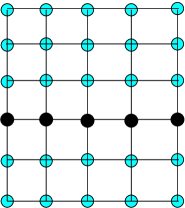
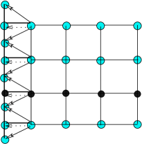
Figure 1: TBA diagrams for the cases  a (left) $G=A_{5},l=4,m=3$,  b (right) $G=B_{5},l=3,m=2$

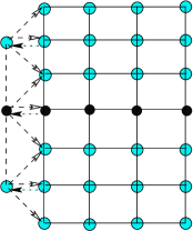
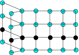
Figure 2: TBA diagrams for the cases  a (left) $G=C_{5},l=2,m=2$,  b (right) $G=D_{7},l=3,m=2$

As one can check, the above $Y$-systems exactly reproduce those which were considered in [15], if one changes $Y_{j}^{a}\rightarrow\left(Y_{j}^{a}\right)^{-1}$. In [15] such $Y$-systems were related to quantum affine Lie algebras $U_{q}(G_{n}^{(1)})$ and their representations. The mathematical meaning standing behind functional $Y$-systems and their relation to representation theory of quantum affine Lie algebras, their character relations and transfer matrix functional relations, is deep and beautiful issue, requiring further investigation. Here we will cite the main result of [15]: the dilogarithm sum rules like (57) corresponding to the ground state of the $Y$-systems we obtained (we omit some technical details and present it in a simplified form relevant for our case):

$$\frac{6}{\pi^{2}}\sum_{a=1}^{n}\sum_{j=1}^{t_{a}l-1}L\left(\frac{X_{j}^{a}}{1+X_{j}^{a}}\right)=\frac{l\dim G_{n}}{l+g}-n,$$ (58)

where $X_{j}^{a}$ satisfy the same functional relations as our $\left(Y_{j}^{a}\right)^{-1}$. Using the relation $L(t)=1-L(1-t)$ and substituting (58) into (57), one can see that the latter reproduce the correct central charge

$$c=\dim G_{n}\left(\frac{l}{l+g}+\frac{m}{m+g}-\frac{l+m}{l+m+g}\right)$$

for all the coset models considered here.

This completes the derivation of TBA $Y$-systems from the S-matrices of relativistic integrable models, and their check by comparison of their ground state thermodynamic with the central charge of their UV limit CFTs. This is one of the most convenient checks of  the S-matrix correctness.

5
Full S-matrix

As we have seen in the previous section, the consistent TBA, which reproduces the correct central charge, dictates unique form of the S-matrix crossing-unitarizing prefactor together with CDD facor, for any pair of two fundamental representations for any algebra $G$. Here we will show that in the cases where the full S-matrix is known for any pair of fundamental representations, i.e. in multiplicity free cases $A_{n},C_{n}$, this prefactor can be calculated from the S-matrix. In the $A_{n}$ case this calculation was done in [11]. The most interesting information one can extract from the above TBA analysis, is the prefactor for $B_{n},D_{n}$ cases. Although  the S-matrix $S_{ab}$ is not know in this cases for any $a,b$, it is known, for example, for spinor-spinor S-matrices: in $B_{n}$ case for $a=b=n$, or in $D_{n}$ case – $a=b=n$ and $a=n,b=n-1$, since then spectral decomposition is multiplicity free. Corresponding rational S-matrices were constructed for PCM in the seminal work [23], but we, unfortunately, don’t know any published trigonometric generalization of their result. It would be interesting to work out corresponding trigonometric S-matrices, especially in their RSOS form relevant in our case.

We recall that our starting S-matrix has the form

$$S_{ab}(\theta)=X_{ab}(\theta)S_{ab}^{(l)}(\theta)\otimes S_{ab}^{(m)}(\theta).$$

The total crossing-unitarizing prefactor $Y_{ab}$ is the product of CDD factor $X_{ab}$ and corresponding crossing-unitarizing prefactors $\sigma_{ab}^{(l)},\sigma_{ab}^{(m)}$ for each $S_{ab}^{(l)}(\theta)$ and $S_{ab}^{(m)}$. As was shown above, the correct TBA derivation, confirming the proper central charge in all the considered cases, was based on the assumption for the crossing-unitaring prefactor form of the full S-matrix (17) with the $\varphi$ having the universal form for all the algebras (42). First, we start with a proof of this statement for $A_{n}$ and $C_{n}$ cases, when the full S-matrix $S_{ab}^{(l,m)}(\theta)$ is known for any pair $a,b$, since being free of multiplicities, the spectral decomposition, and crossing-unitarizing including prefactors $\sigma_{ab}^{(l,m)}$, can be calculated explicitly.

5.1 Vector-vector S-matrices and their fusion

Recall the general RSOS structure of the S-matrix $S_{ab}^{(l)}(\theta)$ for any algebra $G_{n}$. In general one gets $S_{ab}^{(l)}(\theta)$ as a result of fusion procedure starting from the fundamental S-matrix. By fundamental one means the S-matrix for fundamental representations, from which all other representations will appear after decomposition of tensor product of reps into irreducible ones. This representations are usually called the defining representations. The defining reps for $A_{n}$ and $C_{n}$ algebras are their vector representations, while for $B_{n}$ and $D_{n}$ – their spinor ones. In the last case all other fundamental representations can be obtained as a tensor product of spinor ones. But, obtaining the vector representation in the tensor product of spinors, one can get from the vector representation all the others by the same fusion procedure, except for the spinor ones. We don’t know the explicit form of the spinor-spinor trigonometric RSOS S-matrices for $B_{n}$ and $D_{n}$ cases (one can guess they look quite complicated), although they are, as we said, the fundamental S-matrices in these cases. Instead, we will describe vector-vector S-matrices for all the cases. The structure of RSOS S-matrix of the vector-vector representation is well known and described in the literature (see, for example, [24],[6]). We cite it here for completeness and reader convenience, following [25]. It is defined as scattering process of two kinks

$$K_{ac}(\theta_{1})+K_{cd}(\theta_{2})\rightarrow K_{ab}(\theta_{2})+K_{bd}(\theta_{1})$$

connecting different vacua $a,b,c,d\in\Lambda^{\ast}$ of the theory from the weight lattice $\Lambda^{\ast}$ of the algebra $G_{n}$. Weights of its vector representation are

$$\Sigma = \{e_{1}-e_{0},...,e_{n+1}-e_{0}\},\;e_{0}=\frac{\sum_{i=1}^{n+1}e_{i}}{n+1},\;A_{n},$$

$$\Sigma = \{0,\pm e_{1},...,\pm e_{n}\},\;B_{n},$$

$$\Sigma = \{\pm e_{1},...,\pm e_{n}\},\;C_{n},D_{n},$$

where ${e_{i}}$ is some orthonormal basis. Up to a prefactor scalar function $Y$ this kink-kink S-matrix is proportional to the Boltsmann weights (BW) $W$ of statistical lattice models with corresponding symmetry, constructed as solutions of Yang-Baxter interaction round the face equations [24]:

$$S_{11}^{(l)}(\theta_{2}-\theta_{1})=Y(u)W\left(\left.\begin{array}[]{cc}a&b\\ c&d\end{array}\right|f(u)\right)\left(\frac{G_{a}G_{d}}{G_{b}G_{c}}\right)^{f(u)/2},$$ (59)

where $u=(\theta_{2}-\theta_{1})/i\pi,f(u)=cu$ for some constant $c$, $c-a,d-c,b-a,d-b\in\Sigma$, and $G_{a}$ will be defined below. The set of non zero BW for vector-vector representation looks as follows [24]:

$$W\left(\left.\begin{array}[]{cc}a&a+\mu\\ a+\mu&a+2\mu\end{array}\right|u\right) = \frac{\sin(\omega-\lambda u)}{\sin(\omega)}$$ (62)

$$W\left(\left.\begin{array}[]{cc}a&a+\mu\\ a+\mu&a+\mu+\nu\end{array}\right|u\right) = \frac{\sin(a_{\mu\nu}+\lambda u)}{\sin(a_{\mu\nu})}$$ (65)

$$W\left(\left.\begin{array}[]{cc}a&a+\nu\\ a+\mu&a+\mu+\nu\end{array}\right|u\right) = \frac{\sin(\lambda u)}{\sin(\omega)}\left(\frac{\sin(a_{\mu\nu}+\omega)\sin(a_{\mu\nu}-\omega)}{\sin^{2}(a_{\mu\nu})}\right)^{1/2}$$ (68)

($\mu\neq\nu$) for $A_{n}$ case, and

$$W\left(\left.\begin{array}[]{cc}a&a+\mu\\ a+\mu&a+2\mu\end{array}\right|u\right) = \frac{\sin(\lambda-\lambda u)\sin(\omega-\lambda u)}{\sin(\omega)\sin(\lambda)},\;\mu\neq 0$$ (71)

$$W\left(\left.\begin{array}[]{cc}a&a+\mu\\ a+\mu&a+\mu+\nu\end{array}\right|u\right) = \frac{\sin(\lambda-\lambda u)\sin(a_{\mu\nu}+\lambda u)}{\sin(\lambda)\sin(a_{\mu\nu})},\;\mu\neq\pm\nu$$ (74)

$$W\left(\left.\begin{array}[]{cc}a&a+\nu\\ a+\mu&a+\mu+\nu\end{array}\right|u\right) = \frac{\sin(\lambda-\lambda u)\sin(\lambda u)}{\sin(\omega)\sin(\lambda)}\times$$ (77)

$$\times\left(\frac{\sin(a_{\mu\nu}+\omega)\sin(a_{\mu\nu}-\omega)}{\sin^{2}(a_{\mu\nu})}\right)^{1/2}\ \mu \neq \pm\nu$$ (78)

$$W\left(\left.\begin{array}[]{cc}a&a+\nu\\ a+\mu&a\end{array}\right|u\right) = \frac{\sin(\lambda u)\sin(a_{\mu-\nu}+\omega-\lambda+\lambda u)}{\sin(\lambda)\sin(a_{\mu-\nu}+\omega)}\left(G_{a_{\mu}}G_{a_{\nu}}\right)^{1/2}+$$ (81)

$$+\delta_{\mu\nu}\frac{[\lambda-\lambda u][a_{\mu-\nu}+\omega+\lambda u]}{[\lambda][a_{\mu-\nu}+\omega]},\;\mu \neq 0$$

$$W\left(\left.\begin{array}[]{cc}a&a\\ a&a\end{array}\right|u\right) = \frac{\sin(\lambda+\lambda u)\sin(2\lambda-\lambda u)}{\sin(\lambda)\sin(2\lambda)}-\frac{\sin(\lambda-\lambda u)\sin(\lambda u)}{\sin(\lambda)\sin(2\lambda)}J_{a}$$ (84)

for $B_{n},C_{n}$ and $D_{n}$, where $\mu,\nu\in\Sigma,a_{\mu}=\omega(a+\rho)\cdot\mu$, ($\rho$ is the sum of the fundamental weights of the algebra), $a_{0}=-\omega/2,a_{\mu\nu}=a_{\mu}-a_{\nu},a_{\mu-\nu}=a_{\mu}+a_{\nu}$, and the constants $\omega,\lambda$ are defined as

$$\omega=\frac{\pi}{t(g+l)},\lambda=\frac{tg\omega}{2}.$$

Parameter $t=1$ in $A_{n},B_{n},D_{n}$ cases and $t=2$ in $C_{n}$ case. We also used

$$G_{a_{\mu}} = \sigma\frac{s(a_{\mu}+\omega)}{s(a_{\mu})}\prod_{\kappa\neq\pm\mu,0}\frac{\sin(a_{\mu\kappa}+\omega)}{\sin(a_{\mu\kappa})},\;\mu\neq 0,\;G_{a_{0}}=1,$$

$$J_{a} = \sum_{\kappa\neq 0}\frac{\sin(a_{\kappa}+\omega/2-2\lambda)}{\sin(a_{\kappa}+\omega/2)}G_{a_{\kappa}},$$

where $\sigma=-1$ in the $C_{n}$ case and $\sigma=1$ in the $B_{n},D_{n}$ cases. The function $s(x)=\sin(tx)$ in the $B_{n},C_{n}$ cases, and $s(x)=1$ for $D_{n}$. The quantities $G_{a}$ used in (59) are related to $G_{a_{\mu}}$ by $G_{a_{\mu}}=G_{a+\mu}/G_{a}$ and can be written as

$$G_{a}=\varepsilon(a)\prod_{i=1}^{n(+1)}s(a_{i})\prod_{1\leq i<j\leq n(+1)}\sin(a_{i}-a_{j})\sin(a_{i}+a_{j}),$$

where $a=\sum_{i=1}^{n(+1)}a_{i}e_{i}$ defines $a_{i}$, and $\varepsilon(a)$ is a sign factor chosen so that $\varepsilon(a+\mu)/\varepsilon(a)=\sigma$.

The models are called restricted since only the dominant weights

$$a\cdot\theta\leq l$$ (85)

are allowed, where $\theta$ is the highest root of the algebra, and $l$ is the level.

The BW listed above satisfy a set of conditions important for the S-matrix construction:

• unitarity

  $$\sum_{e}W\left(\left.\begin{array}[]{cc}a&e\\ c&d\end{array}\right|u\right)W\left(\left.\begin{array}[]{cc}a&b\\ e&d\end{array}\right|-u\right)=\rho(u)\delta_{bc},$$ (86)

  where in $A_{n}$ case

  $$\rho(u)=\frac{\sin(\omega-\lambda u)\sin(\omega+\lambda u)}{\sin^{2}(\omega)},$$

and in $B_{n},C_{n},D_{n}$ cases

$$\rho(u)=\frac{\sin(\omega-\lambda u)\sin(\omega+\lambda u)\sin(\lambda-\lambda u)\sin(\lambda+\lambda u)}{\sin^{2}(\omega)\sin^{2}(\lambda)},$$ (87)

• crossing symmetry ($B_{n},C_{n},D_{n}$ cases):

  $$W\left(\left.\begin{array}[]{cc}a&b\\ c&d\end{array}\right|u\right)=W\left(\left.\begin{array}[]{cc}c&a\\ d&b\end{array}\right|1-u\right)\left(\frac{G_{b}G_{c}}{G_{a}G_{d}}\right)^{1/2}.$$ (88)

• crossing-unitarity relation ($A_{n}$ case)

  $$\sum_{e}W\left(\left.\begin{array}[]{cc}a&e\\ c&d\end{array}\right|1+u\right)W\left(\left.\begin{array}[]{cc}a&b\\ e&d\end{array}\right|1-u\right)=\delta_{bc}\frac{\sin(\lambda-\lambda u)\sin(\lambda+\lambda u)}{\sin^{2}(\omega)}.$$ (89)

The case $A_{n}$ is different, since vector representation is not conjugate to itself.

Requirements of unitarity and crossing for the S-matrix (59), using (86) and (89) in the $A_{n}$ case, lead to the following functional constraint on the function $Y(u)$, to which we will add two indices $Y_{n,l}(u)$, explicitly emphasizing its dependence on rank $n$ and level $l$:

$$Y_{n,l}(u)Y_{n,l}(-u) = \frac{\sin^{2}(\omega)}{\sin(\omega+\lambda u)\sin(\omega-\lambda u)},$$

$$Y_{n,l}(1+u)Y_{n,l}(1-u) = \frac{\sin^{2}(\omega)}{\sin(\lambda+\lambda u)\sin(\lambda-\lambda u)}.$$

The minimal solution of this system of functional relations (up to so called CDD umbiguities), which has no poles on the physical strip $0<u<1$, was found in [26]:

$$Y_{n,l}(u) = \exp\left\{2\int_{0}^{\infty}\frac{dx}{x}\frac{[\frac{n+1}{2}u]}{[l+n+1][n+1]}\times\right.$$

$$\left.\times\left\{(l)\left(\frac{n+1}{2}u\right)-(n-1+l)\left(\frac{u(n+1)}{2}-n-1\right)\right\}\right\}.$$

We recall that we use the short notations $\left[z\right]=\sinh(xz),\left(z\right)=\cosh(xz)$.

In the same way the functional relations on $Y$ in the $B_{n},C_{n},D_{n}$ cases, using  (86),(88), look like

$$Y(u) = Y(1-u)$$

$$Y(u)Y(-u) = \rho^{-1}(u),$$

where $\rho$ is defined in (87). The minimal solution of this system can be written in terms of  $Y_{n,l}$ (5.1)

$$Y(u)=Y_{tg,tl}(u)Y_{tg,tl}(1-u)\frac{\sin\lambda}{\sin\omega}.$$ (91)

The S-matrices described here can be written in the spectral decomposed form with projectors onto irreducible representations appearing in the tensor product of two vector representations. (These projectors should be written in the IRF form). As was pointed out, the constructed vector-vector S-matrix is pole free and has no bound states. The bound states are produced by insertion of CDD factors, which have poles at the rapidity value corresponding to the desired projector in the spectral decomposition. It is well known that the closed and self consistent bootstrap procedure requires the pole in $S_{11}$ S-matrix in the channel corresponding to the second fundamental weight. Continuation of the bootstrap reproduces massive bound state multiplets corresponding to all the fundamental representations of the algebra. This scenario was proved to be correct in the cases where the spectral decomposition of $S_{ab}$ is known for any $a,b$, and was conjectured to be correct in all the cases. One of the most effective methods of the construction of S-matrix spectral decomposition is the tensor product graph method (TPG). But unfortunately it works only when the spectral decomposition is multiplicity free. This is the situation in the $A_{n},C_{n}$ cases where the tensor product of two representations with fundamental highest weights are multiplicity free.

We briefly recall here the concept of TPG. First of all, there is requirement for the representations, for which we build TPG, to be affinizable (for details see [27],[28]). All the fundamental representations of $A_{n}$ and $C_{n}$ are affinizable. Unfortunately, it is not the case for $B_{n}$ and $D_{n}$ cases. TPG is a graph which is constructed by letting the irreducible components $\lambda$ and $\sigma$ of tensor product $\lambda_{a}\otimes\lambda_{b}$ be the nodes of the graph joined by  a link if $\lambda$ and $\sigma$ have of opposite parity and $\sigma\subset adj\otimes\lambda$. The parity of $\lambda$ is defined to be $\pm 1$ according to whether $\lambda$ appears symmetrically or anti-symmetrically in the tensor product in the limit $q\rightarrow-1$. The concept of TPG works well when TPG is a tree and there are no multiplicities in the tensor product of two representations. In the Tables 1,2 one can find the TPG for any pair of fundamental weights of algebras $A_{n}$ and $C_{n}$.

$\lambda_{a}+\lambda_{b}$

$\rightarrow$

$\lambda_{a+1}+\lambda_{b-1}$

$...$

$\rightarrow$

$\lambda_{a+\min(n+1-a,b)}+\lambda_{b-\min(n+1-a,b)}$

Table 1. Tensor product graph for two fundamental representations $a$ and $b$ of $A_{n}$ ($a\geq b$).

$\lambda_{a}+\lambda_{b}$	$\rightarrow$	$\lambda_{a+1}+\lambda_{b-1}$	$\rightarrow$	$...$	$\lambda_{a+b-1}+\lambda_{1}$	$\rightarrow$	$\lambda_{a+b}$
$\downarrow$		$\downarrow$			$\downarrow$
$\lambda_{a-1}+\lambda_{b-1}$	$\rightarrow$	$\lambda_{a}+\lambda_{b-2}$	$\rightarrow$	$...$	$\lambda_{a+b-2}$
$\downarrow$		$\downarrow$
$\vdots$		$\vdots$
$\lambda_{a-b+1}+\lambda_{1}$	$\rightarrow$	$\lambda_{a-b+2}$
$\downarrow$
$\lambda_{a-b}$

Table 2. Tensor product graph for two fundamental representations $a$ and $b$ of $C_{n}$ ($a\geq b$). For $a+b>n$ the graph truncates at the ($n-a+1$)th column.

Given a TPG, the spectral decomposition of the R-matrix has the form

$$R_{ab}(x)=\sum_{\mu}\rho_{\mu}(x)P_{\mu},$$

where the sum is over the irreps appearing in the tensor product decomposition, i.e. over the nodes of TPG, $x$ is multiplicative spectral parameter, and the main rule dictated by TPG says: if there is an arrow from $\mu$ to $\nu$ on the TPG then the coefficients $\rho_{\mu}(x)$ and $\rho_{\nu}(x)$ satisfy

$$\frac{\rho_{\mu}(x)}{\rho_{\nu}(x)}=\frac{xq^{I(\mu)/2}-x^{-1}q^{I(\nu)/2}}{x^{-1}q^{I(\mu)/2}-xq^{I(\nu)/2}},$$

where

$$x=e^{i\lambda u},\;q=-e^{-i\omega},$$

and the second Casimir $I(\mu)=(\mu+2\rho)\cdot\mu$.

Using these TPG method one can construct the minimal S-matrix for scattering of any two fundamental multiplets of $A_{n}$ and $C_{n}$ [25]. It has the form:

$$S_{ab}^{(l)}(u)=\sigma_{ab}^{(l)}(u)R_{ab}(u),$$

where

$$\sigma_{ab}^{(l)}(u)=Z_{ab}(u)\prod_{j=1}^{a}\prod_{k=1}^{b}Y\left(u+\frac{2j+2k-a-b-2}{tg}\right)$$ (92)

and $Y$ is defined by (5.1) in $A_{n}$ case, and by (91) – in $C_{n}$ case. $Z_{ab}$ coming from the R-matrix, is defined below. The R-matrices have the following form ($b\geq a$)

• $\mathbf{A}_{n}$ case

  $$R_{ab}(u)=\sum_{k=0}^{\min(n+1-b,a)}(-1)^{k+1}\rho_{ab}^{k}(u)P_{\lambda_{b+k}+\lambda_{a-k}}$$

(by definition $\lambda_{n+1}=\lambda_{0}=0$) with

$$\rho_{ab}^{k}(u)=\prod_{p=1}^{k}\frac{\{2p+b-a\}}{\{-2p-b+a\}},$$

and $Z_{ab}$ in this case

$$Z_{ab}(u)=\prod_{j=1}^{a}\prod_{k=1}^{b-1}\{2j+2k-a-b\}\prod_{p=1}^{a}\{-2p-b+a\}.$$ (93)

Here and below we use a new notation

$$\{x\}=\frac{\sin(\omega x/2+\lambda u)}{\sin(\omega)}.$$

• $\mathbf{C}_{n}$ case

  $$R_{ab}(u) = \sum_{j=0}^{\min(n-b,a)}\sum_{k=0}^{a-j}(-1)^{k+j}\rho_{ab}^{jk}(u)P_{\lambda_{b+j-k}+\lambda_{a-j-k}},$$

  $$\rho_{ab}^{jk}(u) = \prod_{p=1}^{j}\frac{\{2p+b-a\}}{\{-2p-b+a\}}\prod_{q=1}^{k}\frac{\{2(n+1)+2q-b-a\}}{\{-2(n+1)-2q+b+a\}},$$

and $Z_{ab}$ in this case

$$Z_{ab}(u) = \left(\frac{\sin\lambda}{\sin\omega}\right)^{ab}\prod_{j=1}^{a}\prod_{k=1}^{b-1}\{2j+2k-a-b\}\{a+b-2(n+1)-2j-2k\}$$ (94)

$$\times\prod_{p=1}^{a}\{-2p-b+a\}\{-2(n+1)-2p+a+b\}.$$

• $\mathbf{B}_{n}$ and $\mathbf{D}_{n}$ cases

In these cases affinizable among fundamental weights representations are only vector and spinor ones, and their tensor products are multiplicity free. We will consider here only S-matrix for two vector representations. It has the following spectral decomposition [23][25]:

$$S_{11}^{(l)}(u)=\{-2\}\{-g\}Y_{g,l}(u)Y_{g,l}(1-u)\left[P_{2\lambda_{1}}-\frac{\{2\}}{\{-2\}}P_{\lambda_{2}}+\frac{\{2\}\{g\}}{\{-2\}\{-g\}}P_{0}\right].$$

5.2 CDD factors

The S-matrices presented above are crossing symmetric, unitary and minimal in the sense that they have no poles in the physical strip. As we said, in order to make bootstrap working, one should multiply these S-matrices by a set of properly chosen CDD factors. They appear as a result of fusion of the CDD factors for vector-vector S-matrices. It is useful to introduce the following notation for universal description of CDD factors

$$\overline{X}(a)=\frac{\sin\left(\frac{\pi}{2}\left(u+\frac{a}{tg}\right)\right)}{\sin\left(\frac{\pi}{2}\left(u-\frac{a}{tg}\right)\right)}.$$

(We recall that $t=1$ in $A,B,D$ cases and $t=2$ in $C$ case.)

• $\mathbf{A}_{n}$ case

Vector-vector S-matrix CDD factor is just $\overline{X}(2)$ and its fusion leads to the following CDD factor for $a,b$ scattering

$$X_{ab}(u)=\prod_{j=|a-b|+1,\;step\;2}^{a+b-1}\overline{X}(j+1)\overline{X}(j-1).$$

One can see that there is a pole in $X_{ab}(u)$ at $u=\frac{a+b}{n+1}$ if $a+b<n+1$, or at $u=2-\frac{a+b}{n+1}$ if $a+b>n+1$. They correspond to particles $a+b$ or $a+b-n-1$ respectively in the direct channel. There is also a pole at $u=\frac{|a-b|}{n+1}$ corresponding to the particle $|a-b|$ in the cross channel. We will not discuss here the double poles, this discussion one can find in [25].

• $\mathbf{C}_{n}$ case

Here the vector-vector CDD factor has the form $X_{11}=\overline{X}(2)\overline{X}(2g-2)$ and its fusion gives

$$X_{ab}(u)=\prod_{j=|a-b|+1,\;step\;2}^{a+b-1}\overline{X}(j+1)\overline{X}(j-1)\overline{X}(2(n+1)-j+1)\overline{X}(2(n+1)-j-1).$$ (95)

As one can see from (95), the pole structure here is more complicated – it exhibits poles up to the 4-th order. Discussion of the S-matrix analytic structure in this case one can find in [25].

• $\mathbf{B}_{n}$ and $\mathbf{D}_{n}$ cases.

CDD factors for the vector-vector S-matrices in these cases has the same form $X_{11}=\overline{X}(2)\overline{X}(2g-2)$.

5.3 Prefactor exponentialization

Now we have to transform both $X_{ab}$ and $\sigma_{ab}^{(l)}$ to the exponential form in order to calculate the quantity $Y_{ab}=$ $\frac{1}{2\pi i}\frac{d}{d\theta}\left(X_{ab}\sigma_{ab}^{(l)}\sigma_{ab}^{(m)}\right)$ used in the TBA calculations.One can use for that the following identity

$$\sin(\pi a)=\exp\left(-\int_{0}^{\infty}\frac{dx}{x}\frac{2\sinh^{2}\left(x\left(a-1/2\right)\right)}{\sinh x}\right)$$

valid for $0<a<1$, and also

$$\frac{\sinh(\lambda(\theta+i\pi\alpha))}{\sinh(\lambda(\theta-i\pi\alpha))}=\exp\left\{-2\int_{0}^{\infty}\frac{dx}{x}\sinh(i\theta x)\frac{\sinh\left(\frac{\pi x}{2}(\frac{1}{\lambda}-2\alpha)\right)}{\sinh\left(\frac{\pi x}{2\lambda}\right)}\right\}$$

valid for $0<\alpha<\frac{1}{\lambda}$. Straightforward but long calculations, using (92),(93),(94),(5.1),(91) lead to the following exponential representations valid in both $A_{n}$ and $C_{n}$ cases:

$$X_{ab}(u) = \exp\left(2\int_{0}^{\infty}\frac{dx}{x}e^{-ux}\left(\delta_{ab}-2\coth x\widetilde{A}_{ab}^{G}(x)\right)\right),$$ (96)

$$\sigma_{ab}^{(l)}(u) = \exp\left(2\int_{0}^{\infty}\frac{dx}{x}e^{-ux}\widetilde{A}_{ab}^{G}(x)\frac{a_{1}^{(g+l)}(x)}{[1]}\right),$$ (97)

where the kernels $\widetilde{A}_{ab}^{G}$ are defined in Appendix and already appeared in the TBA calculations. It turns out that in $B_{n}$ and $D_{n}$ cases the vector-vector S-matrices fit the same general formulas (96),(97). One can see after some simple algebra, that these expressions give a universal answer for the quantity valid in all the cases described above

$$\frac{1}{2\pi i}\frac{d}{d\theta}\ln\left(X_{ab}\sigma_{ab}^{(l)}\sigma_{ab}^{(m)}\right)=\delta_{ab}\delta(\theta)-A_{ab}^{G}\ast\left(A_{g+l,g+l}^{A_{2g+l+m-1}}\right)^{-1},$$

where $\ast$ means convolution. This coincides with the assumption made about the form of $Y_{ab}$ in the TBA calculations of the previous section.

5.4 Special cases of S-matrices

As we mentioned in the introduction, the form of S-matrix (1) includes in it as subclasses S-matrices for other important two dimensional integrable models with Yangian symmetries. One of them are PCM ($l,m\rightarrow\infty$). They are well studied, well defined for any $G=A,B,C,D$ and their S-matrices are self consistent from the bootstrap point of view (see [23]). In particular, there are no double poles unexplainable by Coleman-Thun mechanism. The situation is more subtle with GN models ($l\rightarrow\infty,m=1$). Here the S-matrix conjecture

$$S_{ab}=X_{ab}S_{ab}^{(\infty)},$$ (98)

wich was naively expected to be correct in all the cases $G=A,B,D$ (see the footnote in the introduction about the $C_{n}$ case), was found to suffer from the ”bootstrap violation” [23] in the $B_{n}$ case, while was shown to be correct in the $A$ and $D$ cases. Only recently the $B_{n}$ GN S-matrix was ”corrected” [29] using elegant physical arguments about the symmetry of the Lagrangian. The presence of additional current (compared with $D_{n}$ case) makes the symmetry different, leading to additional RSOS like vacuum degeneracy with additional kink structure. The answer for the S-matrix was shown to be

$$S_{ab}=X_{ab}S_{ab}^{(\infty)}\otimes\widetilde{S}_{ab},$$ (99)

where $\widetilde{S}_{ab}=1$ for any pair ($a,b)$ except for ($n,n)$, when $\widetilde{S}_{nn}=S_{TCI}(\lambda\theta)$ - the RSOS S-matrix of the tricritical Ising model with rescaled rapidity. From the Lie algebraic point of view it is just $A_{1}$ level 2 RSOS model described in the formulas (62). There are some identities and specific features of low level RSOS models. In particular, one can show that $B_{n}$ level 1 RSOS model is identical (up to a rescaling of the spectral parameter $u$) to $A_{1}$ level 2 RSOS model. It is interesting to note that there are the same identities on the level of affine Lie algebras themselves, which were pointed out in the context of generalized parafermions in [31]. In this sense the S-matrix constructed in [29] naturally fits the general form of our S-matrix (1). The identity between (98) and (1) in $A_{n},D_{n}$ cases follows from the fact that RSOS level 1 $A_{n}$ and $D_{n}$ S-matrices are equal to 1 and hence may be ignored in the tensor product of (1).

The same situation  one has with another class of integrable models – low level WZW models perturbed by current-current perturbation. In the most of cases they are equivalent to the GN models – just by fermionization of WZW models (see, e.g. [30]). They are well defined objects, while the GN model are not always well defined: for example, as we said $C_{n}$ GN model cannot be defined on the usual Majorana fermions, but level one $C_{n}$ WZW model with current-current perturbation is well defined and described by the S-matrix (1) with $l\rightarrow\infty,m=1$. Here another interesting identity is valid. Analyzing Boltsmann weights together with the restriction condition (85), one can see the identity (up to a rescaling of the spectral parameter $u$) between $C_{n}$ level 1 and $A_{n-1}$ level 2 RSOS models. This identity, which is absolutely analogous to the relation $(B_{n})_{1}\char 126\relax(A_{1})_{2}$, was also pointed out in [31] for affine Lie algebras.

Both of the identities express themselves also in the form of the TBA diagrams. Looking at the fig 1.b. and at the fig 2.a, in the case $m=1$, one can see that there remains one ”spurious” node under the line of massive nodes on the fig 1.b, and a chain of $n-1$ ”spurious” nodes under the massive line on the fig 2.a. They are nothing but the magnonic degrees of freedom, describing $(A_{1})_{2}$ (TCI) model in the first case, and $(A_{n-1})_{2}$ – in the second. This remark demonstrates how a correct TBA diagram could help to guess the correct S-matrix.

In [25] it was shown, that S-matrix of the form (98) in the $C_{n}$ case sufferes from ”bootstrap violation”: there are double poles unexplainable by the Coleman-Thun mechanism. As we explained, this confusion was related with a naive assumption about the S-matrix form (98), which was expected to be correct for current-current perturbation of the level 1 $C_{n}$ WZW model. The correct form of the S-matrix for this integrable model is $S_{ab}=X_{ab}S_{ab}^{(\infty)}\otimes S_{ab}^{(1)}$ and contains non trivial RSOS tensor factor. As we said, due to the isomorphism $(C_{n})_{1}\char 126\relax(A_{n-1})_{2}$ [31], this factor is physically natural.

6 Discussion

We derived TBA equations from the S-matrices (1) for all the infinite series if Lie algebras $G=A_{n},B_{n},C_{n},D_{n}$. We have shown that with assumption (17) they give the $Y$-systems with the proper high temperature behavior reproducing the correct central charge of the cosets. The assumption (17) was shown to be correct in $A_{n},C_{n}$ cases for any two fundamental multiplets, and also in $B_{n},D_{n}$ cases for vector-vector multiplets scattering.

It would be interesting to obtain crossing-unitarising prefactor for other $B_{n},D_{n}$ trigonometric RSOS S-matrices with available spectral decomposition – spinor-spinor, and vector-spinor ones, in order to be sure in correctness of the assumption (17) also in these cases.

Derivation of  the TBA equations presented in this paper is a technical and quite straightforward procedure. But we think it is not just necessary for completeness of the CFT - TBA relation picture. As we saw, one gets a feedback from this derivation procedure important for the form of the S-matrix itself. An attempt to reduce  the derived TBA system to a known and studied $Y$-system, may give a hint for the correct form of S-matrix. For example, if one would start from the (98) S-matrix for the $B_{n}$ invariant GN model, he will get the $Y$-system with one missing magnonic node on the TBA diagram, compared to the correct one (like Fig. 1b). One immediately realizes what should be added in order to get the correct $Y$-system – tensoring of the S-matrix with RSOS S-matrix of TCI model will give a desired missing magnonic node. This simple logic may be useful in consideration of new, less studied integrable models.

7 Acknowledgements

I am grateful to Roberto Tateo for many useful discussions and stimulating interest to this work. I am also thankful to Changrim Ahn and Doron Gepner for discussions. I thank the Mathematical Department of Durham University for hospitality, where this work was started. The work was supported by NATO grant PST.CLG.980424.

8 Appendix

8.1
Kernels and mass spectrum

Here we list the matrices $\widetilde{A}^{G}$ (inverse matrices for $M_{ab}/\left[t_{ab}^{-1}\right]$)

$\mathbf{A}_{n}$

$$\widetilde{A}_{ab}^{A_{n}}=\frac{\left[\min(a,b)\right]\left[n+1-\max(a,b)\right]}{\left[n+1\right]}.$$ (100)

$\mathbf{B}_{n}$

$$\widetilde{A}_{ab}^{B_{n}} = \frac{\left[\min(a,b)\right]\left(n-\frac{1}{2}-\max(a,b)\right)}{\left(n-\frac{1}{2}\right)},\ a,b\leq n-1,$$ (101)

$$\widetilde{A}_{an}^{B_{n}} = \widetilde{A}_{na}^{B_{n}}=\frac{\left[a\right]}{2\left(n-\frac{1}{2}\right)},\ a\leq n-1,$$

$$\widetilde{A}_{nn}^{B_{n}} = \frac{\left[n\right]}{4\left(n-\frac{1}{2}\right)(1/2)}.$$

$\mathbf{C}_{n}$

$$\widetilde{A}_{ab}^{C_{n}}=\frac{\left[\frac{1}{2}\min(a,b)\right]\left(\frac{1}{2}\left(n+1-\max(a,b)\right)\right)}{\left(\frac{1}{2}\left(n+1\right)\right)}$$ (102)

$\mathbf{D}_{n}\mathbf{.}$

$$\widetilde{A}_{ab}^{D_{n}} = \frac{\left[\min(a,b)\right]\left(n-1-\max(a,b)\right)}{\left(n-1\right)},\ a,b\leq n-2,$$ (103)

$$\widetilde{A}_{an}^{D_{n}} = \widetilde{A}_{an-1}^{D_{n}}=\widetilde{A}_{na}^{D_{n}}=\widetilde{A}_{n-1a}^{D_{n}}=\frac{\left[a\right]}{2\left(n-1\right)},\ a\leq n-2,$$

$$\widetilde{A}_{n-1n-1}^{D_{n}} = \widetilde{A}_{nn}^{D_{n}}=\frac{\left[n\right]}{4\left(1\right)\left(n-1\right)},$$

$$\widetilde{A}_{nn-1}^{D_{n}} = \widetilde{A}_{n-1n}^{D_{n}}=\frac{\left[n-2\right]}{4\left(1\right)\left(n-1\right)},$$

We also list here the kernels $K^{G_{n}}$ (their non zero elements), which are inverse for $A^{G_{n}}$, and differ by a scalar factor from $M_{ab}/\left[t_{ab}^{-1}\right]$:

$\mathbf{A}_{n}$

$$K_{ab}^{A_{n}}=\delta_{ab}-\frac{1}{2(1)}\left(\delta_{a+1,b}+\delta_{a-1,b}\right).$$ (104)

$\mathbf{B}_{n}$

$$K_{ab}^{B_{n}} = K_{ab}^{A_{n}},\ a,b\leq n-1,$$ (105)

$$K_{nn-1}^{B_{n}} = K_{n-1n}^{B_{n}}=-\frac{\left(1/2\right)}{(1)},$$

$$K_{nn}^{B_{n}} = f=\frac{2(1/2)^{2}}{(1)}.$$

$\mathbf{C}_{n}$

$$K_{ab}^{C_{n}} = fK_{ab}^{A_{n}}\left(\frac{\omega}{2}\right),\ a,b\leq n-1,$$ (106)

$$K_{nn-1}^{C_{n}} = K_{n-1n}^{C_{n}}=-\frac{\left(1/2\right)}{(1)},$$

$$K_{nn}^{C_{n}} = 1.$$

$\mathbf{D}_{n}$

$$K_{ab}^{D_{n}} = K_{ab}^{A_{n}},\ a,b\leq n-2,$$ (107)

$$K_{n-1n-2}^{D_{n}} = K_{n-1n}^{D_{n}}=K_{nn-1}^{D_{n}}=K_{n-2n-1}^{D_{n}}=-\frac{1}{2(1)},$$

$$K_{n-1n-1}^{D_{n}} = K_{nn}^{D_{n}}=1.$$

As was mentioned above, mass spectrum vectors $m_{a}$, with components corresponding to masses of different fundamental representation multiplets of algebras $G_{n}$, form eigenvectors of matrices $K^{G_{n}}$ listed above with zero eigenvalues. Here we recall the mass spectra for different algebras

$A_{n}$	$B_{n}$	$C_{n}$	$D_{n}$
$m_{a}=M\sin\frac{\pi a}{n+1}$	$m_{a}=2M\sin\frac{\pi a}{2n-1}$	$M\sin\frac{\pi a}{2(n+1)}$	$m_{a}=2M\sin\frac{\pi a}{2n+2}$
	$(a\leq n-1)$		$(a\leq n-2)$
	$m_{n}=M$		$m_{n-1}=m_{n}=M$

8.2 Solution of (29),(30).

First, we express $\rho_{1}^{n-1}$ using the eq. (27) with $j=1$:

$$\rho_{1}^{n-1}=\sum_{b=1}^{n-1}A_{n-1b}^{A_{n-1}}(\omega/2)\left(\frac{1}{2(1)}\sigma^{b}-\sum_{k=1}^{2l-1}K^{1k}(\omega/2)\widetilde{\rho}_{k}^{b}\right).$$

Hence, using the identity

$$A_{n-1a}^{A_{n-1}}(\omega/2)=f\frac{A_{n-1a}^{C_{n}}}{A_{nn}^{C_{n}}}=2(1/2)\frac{A_{na}^{C_{n}}}{A_{nn}^{C_{n}}},$$

we can write the last term in (30) as

$$D=\frac{1}{2(1)}\rho_{1}^{n-1}=2(1/2)\sum_{a=1}^{n-1}\frac{A_{na}^{C_{n}}}{A_{nn}^{C_{n}}}\left(\frac{1}{2(1)}\sigma^{a}-\sum_{k=1}^{2l-1}K^{1k}(\omega/2)\widetilde{\rho}_{k}^{a}\right).$$

Introducing notations

$$B^{a}=\frac{(1/2)}{(1)}\left(a_{1/2}^{(l)}\sigma^{a}-\widetilde{\rho}_{1}^{a}\right),\ C=\frac{1}{2(1)}\left(a_{1}^{(l)}\sigma^{n}-\widetilde{\rho}_{1}^{n}\right)-D,$$

the system (29),(30) may be written as

$$\sum_{b=1}^{n-1}K_{ab}^{C_{n}}x^{b}-\delta_{a,n-1}\frac{(1/2)}{(1)}x^{n} = B^{a}$$

$$-\frac{(1/2)}{(1)}x^{n-1}+x^{n} = C.$$

Using the last equation, one can express $x^{n}$ and substitute it into the first one getting

$$\sum_{b=1}^{n-1}\left(K_{ab}^{C_{n}}-\delta_{a,n-1}\delta_{b,n-1}\frac{(1/2)^{2}}{(1)^{2}}\right)x^{b}=B^{a}+\delta_{a,n-1}\frac{(1/2)}{(1)}C.$$

The matrix in the l.h.s. has as an inverse the restriction of $A_{ab}^{C_{n}}$ to the values $a,b\leq n-1$, and we have the solution:

$$x^{a}=A_{an-1}^{C_{n}}\frac{(1/2)}{(1)}C+\sum_{b=1}^{n-1}A_{ab}^{C_{n}}B^{b}.$$

Using the obtained $x^{n-1}$ in the second equation, we get

$$x^{n}=A_{nn}^{C_{n}}C+\frac{(1/2)}{(1)}\sum_{b=1}^{n-1}A_{n-1b}^{C_{n}}B^{b},$$

where we used the identity

$$A_{n-1n-1}^{C_{n}}\frac{(1/2)^{2}}{(1)^{2}}+1=A_{nn}^{C_{n}}.$$

Explicit use of  the definitions of $B^{a},C,D$ gives the expressions we used in the main text.

8.3 Solution of (36) - (38).

We solve (35) with respect to $x^{n}$

$$x^{n}=\frac{1}{2(1/2)}\left(a_{1/2}^{(l)}\sigma^{n}-\widetilde{\rho}_{1}^{n}\right)-\frac{1}{f}K_{n,n-1}^{B_{n}}x^{n-1},$$

and substitute it into (34). We get an equation, which together with (33), can be written as

$$\sum_{b=1}^{n-1}\left(K_{ab}^{B_{n}}-\delta_{a,n-1}\delta_{b,n-1}\frac{1}{f}\left(K_{n,n-1}^{B_{n}}\right)^{2}\right)x^{b}=B^{a}+\delta_{a,n-1}\frac{1}{2(1)}C,$$ (108)

where

$$B^{a} = \frac{1}{2(1)}\left(a_{1}^{(l)}\sigma^{a}-\widetilde{\rho}_{1}^{a}\right),$$

$$C = a_{1/2}^{(l)}\sigma^{n}-\widetilde{\rho}_{1}^{n}-\rho_{1}^{n}.$$

The inverse matrix for the one in the parenthesis in the l.h.s. of (108) coincides with $A_{ab}^{B_{n}}$, and we get

$$x^{a}=\sum_{b=1}^{n-1}A_{ab}^{B_{n}}B^{b}+A_{an-1}^{B_{n}}C$$

One can now substitute $x^{n-1}$ in the last form into $x^{n}$ and get finally the expressions (39)(40), after collection of similar terms, using the kernel identity $A_{an-1}^{B_{n}}=2(1/2)A_{an}^{B_{n}}$, valid for $a\leq n-1$.

References

- [1] F.Ravanini Phys. Let. B282 (1992) 73, hep-th/9202020.
- [2] E.Quattrini, F.Ravanini, R.Tateo, in ”Quantum Field Theory and String Theory”, NATO ASI Series B: Physics v.328, (1995) 273, hep-th/931116.
- [3] R.Tateo, Int. J. Mod. Phys. A10 (1995) 1357, hep-th/9405197.
- [4] P.Dorey, R.Tateo, K.E.Thompson, Nucl. Phys. B470 (1996) 317, hep-th/9601123.
- [5] P.Dorey, A.Pocklington, R.Tateo, Nucl. Phys. B661 (2003) 464, hep-th/0208202.
- [6] V.V.Bazhanov, N.Reshetikhin, J. of Phys. A: Math. Gen. 23 (1990) 1477, Prog. of Theor. Phys. Supp. 102 (1990) 301.
- [7] A.Kuniba, Nucl. Phys. B389 (1993) 209.
- [8] A.Kuniba, T.Nakanishi, J.Suzuki, Int. J. Mod. Phys. A9 (1994) 5215 hep-th/9309137, 5267 hep-th/9310060, A.Kuniba, J.Suzuki, Com. Math. Phys. 173 (1995) 225 hep-th/9406180.
- [9] C.Destri, H.J. de Vega, J. of Phys. A: Math. Gen. 22 (1989) 1329, Nucl. Phys. B374 (1992) 692, Nucl. Phys. B385 (1992) 361.
- [10] N.Yu.Reshetikhin, H.Saleur, Nucl. Phys. B419 (1994) 507, hep-th/9309135.
- [11] T.J.Hollowood, Phys. Let. B320 (1994) 43, hep-th/9308147.
- [12] P.Fendley, Phys. Rev. B63 (2001) 104429, cond-mat/0008372; JHEP 0105 (2001) 050, hep-th/0101034.
- [13] A.Babichenko, R.Tateo, Phys. Let. B573 (2003) 239, hep-th/0307009.
- [14] C.Ahn, D.Bernard, A.LeClair, Nucl. Phys. B346 (1990) 409.
- [15] A.Kuniba, T.Nakanishi, Mod. Phys. Let. A7 (1992) 3487, hep-th/9206034.
- [16] H.W.Braden, E.Corrigan, P.E.Dorey, R.Sasaki, Nucl. Phys. B338 (1990) 689, B356 (1991) 469.
- [17] P.Dorey, Nucl. Phys. B358 (1991) 654.
- [18] G.W.Delius, M.T.Grisaru, D.Zanon, Nucl. Phys. B382 (1992) 365, hep-th/9201067.
- [19] N.Yu.Reshetikhin, P.B.Wiegmann, Phys. Let. B189 (1987) 125.
- [20] Al.B.Zamolodchikov, Nucl. Phys. B342 (1990) 695, B358 (1991) 497, B366 (1991) 122.
- [21] T.R.Klassen, E.Melzer, Nucl. Phys. B338 (1990) 485, B350 (1991) 635.
- [22] M.J.Martins Phys. Let. B277 (1992) 301; Nucl. Phys. B394 (1993) 339.
- [23] E.Ogievetsky, N.Reshetikhin, P.Wiegmann, Nucl. Phys. B280 (1987) 45.
- [24] M.Jimbo, T.Miwa, M.Okado, Com. Math. Phys. 116 (1988) 507.
- [25] T.J.Hollowood, Nucl. Phys. B414 (1994) 379, hep-th/9305042.
- [26] H.J. de Vega, V.A.Fateev, Int. J. Mod. Phys. A6 (1991) 3221.
- [27] N.J.MacKay, J. Phys. A: Math. Gen A24 (1991) 4017; J. Phys. A: Math. Gen A25 (1992) L1343.
- [28] R.B.Zhang, M.D.Gould, A.J.Bracken, Nucl. Phys. B354 (1991) 625.
- [29] P.Fendley, H.Saleur, Phys. Rev. D65 (2002) 025001 hep-th/0105148.
- [30] P.Di Francesco, P. Mathieu, D. Senechal, ”Conformal Field Theory”, Springer-Verlag, New York (1997).
- [31] D.Gepner, Nucl. Phys. B290 (1987) 10.