The DIAGONAL AFFINE COSET CONSTRUCTION OF THE ${\mathbb{Z}}_{k}$ PARAFERMION HALL STATES

Abstract

We construct the ${\mathbb{Z}}_{k}$ parafermions as diagonal affine cosets and apply them to the quantum Hall effect. This realization is particularly convenient for the analysis of the ${\mathbb{Z}}_{k}$ pairing rules, the modular $S$-matrices, the $W_{k}$ symmetry and quantum group symmetry. The results are used for the computation of the mesoscopic chiral persistent currents in presence of Aharonov–Bohm flux.

1 Introduction

Read and Rezayi [1] have described a new hierarchy of incompressible Hall states in the second Landau level with filling factors

$$\nu_{k}=2+\frac{k}{k+2},\quad k=2,3,4\ldots$$ (1)

which have been observed later in an experiment [2] with thermal activation of quasiparticle–quasihole pairs in extremely high mobility samples. The exact quantization of the Hall conductance $\sigma_{H}=\nu(e^{2}/h)$ for filling factors $\nu=5/2$ and $8/3$ ($k=2$ and $4$) was obvious while at $\nu=13/5$ and $19/7$, ($k=3$ and $5$) there were only well-expressed nonzero minimums of the resistance.

The two-dimensional conformal field theory (CFT) has been successfully applied for the description of the dynamics of the edge excitations in the fractional quantum Hall (FQH) states. Due to the bulk incompressibility in the FQH sample the effective large-scale field theory turns out to be a $(2+1)$ dimensional Chern–Simons theory [3] (say, on a dense cylinder) which is known to be equivalent to a $(1+1)$ dimensional CFT (on a cylinder). Thus, the universality classes of the incompressible FQH states can be ultimately labeled by unitary rational conformal field theories (RCFT).

The RCFT for the parafermion FQH states with filling factors (1) has been originally formulated [1] in terms of a $u(1)$ boson describing the electric properties and the ${\mathbb{Z}}_{k}$ parafermionic CFT describing the neutral degrees of freedom. The ground state wave function is realized as [1]

$$\Psi_{\mathrm{GS}}(z_{1},\ldots,z_{N})=\prod_{1\leq a<b\leq N}(z_{a}-z_{b})^{1+\frac{2}{k}}\quad\langle\Psi_{1}(z_{1})\cdots\Psi_{1}(z_{N})\rangle$$ (2)

where $\Psi_{1}$ is the first among the ${\mathbb{Z}}_{k}$-parafermion currents $\Psi_{i}$ for $i=1,\ldots,k-1$ with CFT dimensions $\Delta_{i}=i(k-i)/k$, and the following operator product expansion [4]

$$\Psi_{i}(z)\Psi_{j}(w)\sim\left(z-w\right)^{-\frac{2ij}{k}}\Psi_{i+j}(w),\quad i+j<k,$$

$$\Psi_{i}(z)\Psi^{*}_{j}(w)\sim\left(z-w\right)^{-\frac{2j(k-i)}{k}}\Psi_{i-j}(w).\quad i<j$$

In this paper we focus on an alternative realization of the ${\mathbb{Z}}_{k}$ parafermions in terms of a diagonal affine coset [5] which turns out to be more natural for the parafermion FQH states.

2 The RCFT for the ${\mathbb{Z}}_{k}$ parafermion FQHE

The RCFT for the ${\mathbb{Z}}_{k}$ parafermion FQH states has the same structure like the original one as formulated in Ref. [1]

$$\left(\widehat{u(1)}\oplus\mathrm{PF}_{k}\right)^{{\mathbb{Z}}_{k}},\quad\mathrm{PF}_{k}=\frac{\widehat{su(k)_{1}}\oplus\widehat{su(k)_{1}}}{\widehat{su(k)_{2}}}.$$ (3)

However, now the ${\mathbb{Z}}_{k}$ parafermions are realized as a diagonal affine coset denoted as $\mathrm{PF}_{k}$ and we have used the superscript ${\mathbb{Z}}_{k}$ to denote a ${\mathbb{Z}}_{k}$ selection rule coupling the electric and neutral sectors of the theory. This rule can be formulated as follows: the edge excitations for the parafermion FQH system are represented by certain primary conformal fields which are labeled by pairs of the $u(1)$ charge $\lambda$ and the parafermion primary fields $\Phi$

$$(\lambda,\Phi)\ \Rightarrow\ :\mathrm{e}^{2\pi i\frac{\lambda}{\sqrt{k(k+2)}}\phi(z)}:\otimes\ \Phi(z),\quad\Phi(z)\in\mathrm{PF}_{k}^{*}.$$

Then the ${\mathbb{Z}}_{k}$ paring rule (PR) states that an excitation labeled by $(\lambda,\Phi)$ is admissible only if

$$P\left[\Phi\right]=\lambda\mod\ k,$$ (4)

where $P$ is the parafermion ${\mathbb{Z}}_{k}$-charge [4, 5]. The topological order of the parafermion states, which is an important characteristics of any FQH state and gives basically the number of the topologically inequivalent excitations, in this case is [5]

$$\mathrm{TO}=\frac{(k+1)(k+2)}{2}.$$

It is instructive to note that the complete parafermion CFT (3) can be obtained by projecting neutral degrees of freedom in a maximally symmetric chiral quantum Hall lattice (in the terminology of Ref.  [3]) denoted by the symbol $(3|{}^{1}A_{k-1}\,{}^{1}A_{k-1})$ that reproduces [5] the same filling factor (1). The structure of this $K$-matrix theory corresponds to the left hand side of

$$\left(\widehat{u(1)}\oplus\widehat{su(k)_{1}}\oplus\widehat{su(k)_{1}}\right)^{{\mathbb{Z}}_{k}}\ \simeq\ \left(\widehat{u(1)}\oplus\frac{\widehat{su(2)_{k}}}{\widehat{u(1)}}\oplus\widehat{su(k)_{2}}\right)^{{\mathbb{Z}}_{k}}$$

while the $\widehat{su(k)_{2}}$ current algebra in the right hand side expresses the layer (or flavor) symmetry of $k$ pairs of Dirac–Weyl fermions that could be gauged away without changing the filling factor since the subalgebra $\widehat{su(k)_{1}}\oplus\widehat{su(k)_{1}}$ is completely decoupled from the electric charge. This projection provides a constructive way to obtain a non-abelian theory from an abelian parent (the latter being identified within the ADE classification of abelian FQH states [3]). It is worth-noting that the PR appears naturally [5] in the abelian parent CFT and is preserved by the coset projection so that the projected theory inherits it.

3 The diagonal coset $\mathrm{PF}_{k}$

In this section we shall analyse in more detail the affine coset

$$\mathrm{PF}_{k}=\frac{\widehat{su(k)_{1}}\oplus\widehat{su(k)_{1}}}{\widehat{su(k)_{2}}}.$$ (5)

The currents in the $\widehat{su(k)_{2}}$ algebra in the denominator of the coset are defined as

$$J^{a}=J^{a}_{1}+J^{a}_{2}\in\widehat{su(k)_{2}},\quad\mathrm{where}\quad J^{a}_{1}\in\widehat{su(k)_{1}}^{(1)},\quad J^{a}_{1}\in\widehat{su(k)_{1}}^{(2)}$$ (6)

and the superscript $(1)$ or $(2)$ refers to the first or the second copy of $\widehat{su(k)_{1}}$ in the numerator of $\mathrm{PF}_{k}$ respectively. That is why this type of cosets are called the “diagonal” cosets.

The stress tensor of the coset CFT (5) is constructed according to the standard Goddard–Kent–Olive procedure [7]

$$T(z)=T^{\widehat{su(k)_{1}}\oplus\widehat{su(k)_{1}}}(z)-T^{\widehat{su(k)_{2}}}(z)$$ (7)

and its modes satisfy the Virasoro algebra with central charge

$$c_{k}=c^{(1)}+c^{(1)}-c^{(2)}=\frac{2(k-1)}{k+2},$$ (8)

which is exactly the central charge of the ${\mathbb{Z}}_{k}$ parafermion CFT [4]. Note that the stress tensor (7) commutes with all currents in the $\widehat{su(k)_{2}}$ subalgebra which allows us to interpret the latter as a gauge symmetry.

The primary fields of the coset $\mathrm{PF}_{k}$ can be labeled generically by triples $(\underline{\Lambda},\underline{\Lambda}^{\prime};\underline{\Lambda}^{\prime\prime})$ of SU(k) weights: two level-1 weights $\underline{\Lambda}$ and $\underline{\Lambda}^{\prime}$ for the two copies of $\widehat{su(k)_{1}}$ in the numerator and one level-2 weight $\underline{\Lambda}^{\prime\prime}$ for the $\widehat{su(k)_{2}}$ in the denominator. Not all combinations of weights are allowed [6]—they must satisfy the following selection rule (conservation of $k$-ality)

$$[\underline{\Lambda}]+[\underline{\Lambda}^{\prime}]=[\underline{\Lambda}^{\prime\prime}],\quad\mathrm{where}\quad[\underline{\Lambda}]=\sum_{i=1}^{k-1}i\lambda^{i}\quad\mathrm{for}\quad\underline{\Lambda}=\sum_{i=1}^{k-1}\lambda^{i}\underline{\Lambda}_{i},$$

$\underline{\Lambda}_{i}$ are the fundamental weights for $SU(k)$ and $\lambda^{i}$ the Dynkin labels corresponding to the general weight $\underline{\Lambda}$. Since the admissible $\widehat{su(k)_{1}}$ weights are the fundamental weights $\underline{\Lambda}_{\mu}$ ($0\leq\mu\leq k-1$; $\underline{\Lambda}_{0}=0$) and any admissible $\widehat{su(k)_{2}}$ weight can be written as a sum of two fundamental weights, $\underline{\Lambda}_{\mu}+\underline{\Lambda}_{\rho}$, ($0\leq\mu\leq\rho\leq k-1$) the admissible triples should have the form

$$(\underline{\Lambda}_{\mu},\ \underline{\Lambda}_{\rho};\ \underline{\Lambda}_{\mu+\sigma}+\underline{\Lambda}_{\rho-\sigma}),\quad\mu,\rho,\sigma=0,\ldots,k-1.$$ (9)

Next, not all admissible triples give inequivalent primary fields of the coset. The action of the simple currents [6]

$$J(\underline{\Lambda}_{\mu})=\underline{\Lambda}_{(\mu+1\mod k)}$$ (10)

which are outer automorphisms of the Dynkin diagrams, permuting the Dynkin labels as illustrated on Fig. 1, commutes with the coset stress tensor while not commuting with those of the numerator and denominator separately.

Figure 1: Under the action of the simple current $J$ the Dynkin labels are rotated counter-clockwise, i.e., $\lambda^{1}\to\lambda^{2},\ldots,\lambda^{k-2}\to\lambda^{k-1}$, $\lambda^{k-1}\to\lambda^{0}$ and $\lambda^{0}\to\lambda^{1}$ .

As a result the triples which can be connected by the action of the simple currents are equivalent and represent the same irreducible representation (IR) of the coset. This is known as the field identification [6]

$$\left(J(\underline{\Lambda}),\ J(\underline{\Lambda}^{\prime});\ J(\underline{\Lambda}^{\prime\prime})\right)\simeq\left(\underline{\Lambda},\ \underline{\Lambda}^{\prime}\ ;\ \underline{\Lambda}^{\prime\prime}\right).$$

Acting with the simple current (10) on the admissible triples (9) we get the following triple identification

$$(\underline{\Lambda}_{\mu+\gamma},\ \underline{\Lambda}_{\rho+\gamma};\ \underline{\Lambda}_{\mu+\sigma+\gamma}+\underline{\Lambda}_{\rho-\sigma+\gamma})\simeq(\underline{\Lambda}_{\mu},\ \underline{\Lambda}_{\rho};\ \underline{\Lambda}_{\mu+\sigma}+\underline{\Lambda}_{\rho-\sigma}).$$ (11)

Choosing $\gamma$ in the above relation such that $\rho+\gamma=0\mod k$ one can always eliminate the second weight, which is our canonical choice of representative for the IR’s of the coset. In this case the $\widehat{su(k)_{2}}$-weight $\underline{\Lambda}^{\prime\prime}$ completely determines the triple since the first $\widehat{su(k)_{1}}$ weight is uniquely determined by its $k$-ality, which should match the $k$-ality of the level-2 weight

$$\mathrm{\bf IR^{\prime}s:}\quad\underline{\Lambda}_{\mu}+\underline{\Lambda}_{\rho}\quad\Longleftrightarrow\quad(\underline{\Lambda}_{\mu+\rho},\ \underline{\Lambda}_{0};\ \underline{\Lambda}_{\mu}+\underline{\Lambda}_{\rho}),\quad 0\leq\mu\leq\rho\leq k-1.$$ (12)

Now the parafermion ${\mathbb{Z}}_{k}$ charge is simply

$$P[\underline{\Lambda}_{\mu}+\underline{\Lambda}_{\rho}]=\mu+\rho\mod k.$$ (13)

The definition of the coset stress tensor (7) as the difference between two other stress tensors gives the following formula for the conformal dimensions

$$\Delta(\underline{\Lambda},\underline{\Lambda}^{\prime};\underline{\Lambda}^{\prime\prime})=\Delta^{(1)}(\underline{\Lambda})+\Delta^{(1)}(\underline{\Lambda}^{\prime})-\Delta^{(2)}(\underline{\Lambda}^{\prime\prime})\mod{\mathbb{Z}}$$ (14)

which reproduces only the fractional part of the CFT dimension. Note that for some triples the level-2 weight $\underline{\Lambda}^{\prime\prime}$ may have bigger positive CFT dimension than the sum of the CFT dimensions of $\underline{\Lambda}$ and $\underline{\Lambda}^{\prime}$ in which case the total CFT dimension would appear to be negative, however, this is not the case. That is why “$\mod{\mathbb{Z}}$” in Eq. (14) is necessary and important. Thus obtaining the correct CFT dimensions of the coset primary fields is usually indirect and non-trivial. However, for this particular diagonal coset, using the field identification (11) and choosing appropriate representatives (different from the canonical ones) one can prove [5] the following exact formula for the CFT dimensions of the coset IR’s

$$\Delta^{\mathrm{PF}}(\underline{\Lambda}_{\mu}+\underline{\Lambda}_{\rho})=\frac{\mu(k-\rho)}{k}+\frac{(\rho-\mu)(k-\rho+\mu)}{2k(k+2)},\quad 0\leq\mu\leq\rho\leq k-1.$$ (15)

The characters of the diagonal coset

$$\mathrm{ch}_{\underline{\Lambda}_{\mu}+\underline{\Lambda}_{\rho}}(\tau)=\mathop{\mathrm{tr}}_{\qquad\quad{\mathcal{H}}_{\underline{\Lambda}_{\mu}+\underline{\Lambda}_{\rho}}}q^{L_{0}-c/24},\quad q=\mathrm{e}^{2\pi i\tau}\quad(\mathrm{Im}\,\tau>0)$$

where $L_{0}$ is the zero modes of the stress tensor (7) and ${\mathcal{H}}_{\underline{\Lambda}_{\mu}+\underline{\Lambda}_{\rho}}$ is the IR with label $\underline{\Lambda}_{\mu}+\underline{\Lambda}_{\rho}$, can be written in the form of the so called universal chiral partition functions with statistical matrix equal to the inverse Cartan matrix $C^{-1}$ for $SU(k)$

$$\mathrm{ch}^{Q}_{\sigma}(\tau;\mathrm{PF}_{k})=q^{\Delta_{\sigma}-c_{k}/24}\sum\limits_{\mathop{m_{1},m_{2},\ldots,m_{k-1}=0}\limits_{\sum\limits_{i=1}^{k-1}\,i\,m_{i}\equiv Q\mod k}}^{\infty}\frac{q^{\underline{m}.C^{-1}.\left(\underline{m}-\underline{\Lambda}_{\sigma}\right)}}{(q)_{m_{1}}\cdots(q)_{m_{k-1}}},$$ (16)

where $(q)_{n}=\prod\limits_{j=1}^{n}(1-q^{j})$, $c_{k}$ is given by Eq. (8) and $\Delta_{\sigma}=\Delta^{\mathrm{PF}}(\underline{\Lambda}_{0}+\underline{\Lambda}_{\sigma})$ is computed from Eq. (15) for $\sigma=0,\ldots,k-1$. The independent characters are labeled by $(\sigma,Q)$ with $0\leq\sigma\leq Q\leq k-1$ and the relation between these new labels and the old ones is $Q=\rho$, $\sigma=\rho-\mu$.

4 The modular $S$-matrix for the diagonal coset

The $S$ transformation of the modular parameter $\tau^{\prime}=-1/\tau$ (like in any RCFT) leads to the following linear transformation of the characters

$$\mathrm{ch}_{\underline{\Lambda}_{\mu}+\underline{\Lambda}_{\nu}}(\tau^{\prime})=\sum_{0\leq\rho\leq\sigma\leq k-1}{\mathop{S}\limits^{\circ}}_{\underline{\Lambda}_{\mu}+\underline{\Lambda}_{\nu};\ \underline{\Lambda}_{\rho}+\underline{\Lambda}_{\sigma}}\quad\mathrm{ch}_{\underline{\Lambda}_{\rho}+\underline{\Lambda}_{\sigma}}(\tau)$$

where ${\mathop{S}\limits^{\circ}}$ is the coset $S$ matrix. Using the standard Goddard-Kent-Olive procedure for finding the $S$ matrix of the coset we obtain ${\mathop{S}\limits^{\circ}}$ as a product of the $S$ matrix of the numerator of the coset (5) and the inverse transposed $S$ matrix of the denominator [7]. Since the numerator is a direct sum of algebras the $S$ matrices for both factors have to be multiplied, however, if we use only canonical triples (12) the second weight $\underline{\Lambda}^{\prime}=0$ corresponds to the vacuum sector so that the second $S$ matrix becomes a simple normalization factor $1/\sqrt{k}$. The first $S$ matrix, which is of a rational $u(1)^{k-1}$ torus type, is completely determined from the $k$-alities of the labels of $\widehat{su(k)_{2}}$ in the denominator. Finally, since the $S$ matrix for $\widehat{su(k)_{2}}$ is unitary we get the following expression for the coset $S$ matrix:

$${\mathop{S}\limits^{\circ}}_{\underline{\Lambda}_{\mu}+\underline{\Lambda}_{\nu};\ \underline{\Lambda}_{\rho}+\underline{\Lambda}_{\sigma}}={\exp\left(2\pi i\frac{(\mu+\nu)(\rho+\sigma)}{k}\right)}\ \left({S^{(2)}_{\underline{\Lambda}_{\mu}+\underline{\Lambda}_{\nu};\ \underline{\Lambda}_{\rho}+\underline{\Lambda}_{\sigma}}}\right)^{*}$$ (17)

where the label’s parameters satisfy $\ 0\leq\mu\leq\nu\leq k-1$, $0\leq\rho\leq\sigma\leq k-1$. Recall that the $S$ matrix for $\widehat{su(k)_{2}}$ can be computed using Kac formula [7]

$$S^{(2)}_{\underline{\Lambda};\ \underline{\Lambda}^{\prime}}=\frac{i^{\,k(k-1)/2}}{\sqrt{k(k+2)^{k-1}}}\sum_{w\in\mathcal{W}}\epsilon(w)\ \exp\left(-2\pi i\frac{\left(\underline{\Lambda}+\underline{\rho}\left|w(\underline{\Lambda}^{\prime}+\underline{\rho})\right)\right.}{k+2}\right),$$

where $\mathcal{W}$ is the Weyl group of $SU(k)$, $\epsilon(w)$ is the determinant of the element $w\in\mathcal{W}$ and $\underline{\rho}$ is the Weyl vector [7].

Given the explicit coset $S$ matrix (17), the fusion rules can be obtained by the Verlinde formula [7], however, as can be seen from Eq. (17) the coset $S$ matrix differs from the (conjugated) $S$ matrix for $\widehat{su(k)_{2}}$ only by a phase. This phase can be interpreted as the action of simple currents on $S^{(2)}$. Since the charge conjugation and the simple currents are automorphisms they preserve the fusion rules. Thus we conclude that the fusion rules for the diagonal coset are the same as those for $\widehat{su(k)_{2}}$. In particular there are primary fields which obey non-abelian statistics [5].

5 $W_{k}$ symmetry

The $\widehat{su(k)_{2}}$ currents which are gauged away in the diagonal coset (5) commute with all independent polynomial Casimir operators of $SU(k)$ which generate a $W_{k}$ algebra. Therefore, after removing all dimension-one currents, the coset (5) can be completely characterized by its $W_{k}$ symmetry [5]. The central charge (8) of the diagonal coset coincides with that for the $W_{k}$ unitary minimal models with the lowest possible parameter $p=k+1$. To make this relation more transparent we shall identify the Fateev–Lukyanov weight $\beta$ within the Coulomb gas approach to the ${\mathbb{Z}}_{k}$ parafermions [4] with the weights of the diagonal coset [5]

$$\beta=\alpha_{+}\underline{\Lambda}^{(1)}+\alpha_{-}\underline{\Lambda}^{(2)}=-\frac{k+1}{\sqrt{(k+1)(k+2)}}\left(\underline{\Lambda}_{\mu}+\underline{\Lambda}_{\rho}\right),$$

where, using canonical triples (12) only, we have set $\underline{\Lambda}^{(1)}=0$ and the Coulomb gas parameters are determined by

$$\alpha_{+}+\alpha_{-}=\alpha_{0},\quad\alpha_{+}\alpha_{-}=-1,\quad(\alpha_{0})^{2}=\frac{1}{(k+1)(k+2)}.$$

The explicit form of the $W_{k}$ generators can be given by using the quantum Miura transformation [5].

6 Quantum group structure of $\mathrm{PF}_{k}$

The triples equivalence (11) and the canonical choice (12) demonstrate that there is a 1–1 correspondence between the IRs of $\mathrm{PF}_{k}$ and $\widehat{su(k)_{2}}$: both labeled by $\underline{\Lambda}_{\mu}+\underline{\Lambda}_{\rho}$ (this is not obvious in the $\widehat{su(2)_{k}}/\widehat{u(1)}$ realization of the ${\mathbb{Z}}_{k}$ parafermions). Furthermore, Eq. (17) proves that both $S$-matrices are equivalent since they are related by charge conjugation and the action of simple currents. These two facts almost prove that the quantum group for the coset (5) is the same as that for $\widehat{su(k)_{2}}$, i.e., [8]

$$U_{q}\left(sl(k)\right)\quad\mathrm{with}\quad q=\exp\left(-i\frac{\pi}{k+2}\right),\quad{\lfloor m\rfloor}_{q}=\frac{q^{m}-q^{-m}}{q^{1}-q^{-1}}.$$

7 Application: persistent currents in the ${\mathbb{Z}}_{k}$ parafermion quantum Hall states

When mesoscopic FQH disk samples are threaded by Aharonov–Bohm flux, the derivative of the free energy $F(T,\phi)=-k_{B}T\ln Z(T,\phi)$, with respect to the magnetic flux $I(T,\phi)=-\partial_{\phi}F(T,\phi)$, gives rise to equilibrium persistent currents, which are observable

$$I(T,\phi)=\frac{e}{h}\,k_{B}T\frac{\partial}{\partial\phi}\ln Z(\tau,\phi\tau),\quad Z(\tau,\zeta)=\mathop{\mathrm{tr}}_{\quad{\mathcal{H}}}q^{L_{0}-c/24}\ \mathrm{e}^{2\pi i\zeta J_{0}},$$

whre $J_{0}$ is the electric charge operator. The precise thermodynamic identification of the modular parameters is given [10] in terms of the absolute temperature $T$ and the (dimensionless) Aharonov–Bohm flux $\phi=\Phi/(h/e)$

$$q=\mathrm{e}^{2\pi i\tau},\quad\tau=i\pi\frac{T_{0}}{T},\quad\zeta=\phi\tau,\quad T_{0}=\frac{\hbar v_{F}}{\pi k_{B}L},\quad\phi\in{\mathbb{R}}.$$

The complete chiral CFT partition function for the ${\mathbb{Z}}_{k}$ parafermion FQH states is constructed as the sum of the characters of all inequivalent IRs [10]

$$Z_{k}(\tau,\zeta)=\mathrm{e}^{-{\pi}\nu_{H}\frac{\left(\mathrm{Im}\,\zeta\right)^{2}}{\mathrm{Im}\,\tau}}\sum_{l\mod k+2}\quad\sum_{\rho\geq l-\rho\mod k}\chi_{l,\rho}(\tau,\zeta),$$

where, following Ref. [9], a non-holomorphic exponential factor in front of the sum has been included in order to restore the invariance of the FQH system under the Laughlin spectral flow. The complete IR’s characters [5]

$$\chi_{l,\rho}(\tau,\zeta)=\sum_{s=0}^{k-1}K_{l+s(k+2)}(\tau,k\zeta;k(k+2))\mathrm{ch}\left(\underline{\Lambda}_{l-\rho+s}+\underline{\Lambda}_{\rho+s}\right)(\tau)$$

are special combinations (satisfying the ${\mathbb{Z}}_{k}$ pairing rule (4)) of the characters of the $u(1)$ sector describing the electric/magnetic properties of the FQH system

$$K_{l}(\tau,\zeta;m)=\frac{1}{\eta(\tau)}\sum_{n\in{\mathbb{Z}}}q^{\frac{m}{2}(n+\frac{l}{m})^{2}}\ \mathrm{e}^{2\pi i\zeta(n+\frac{l}{m})},\quad\eta(\tau)=q^{\frac{1}{24}}\prod_{n=1}^{\infty}(1-q^{n})$$

and the neutral characters (16) of the diagonal coset $\mathrm{PF}_{k}$. Using these explicit formulas we have computed numerically [10] the chiral persistent currents for the ${\mathbb{Z}}_{k}$ parafermion FQH states with $k=2,3$ and $4$ for temperatures in the range $0.03\leq T/T_{0}\leq 14$. As illustrated on Fig. 2

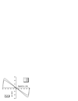
Figure 2: Persistent currents in the $k=2,3$ and $4$ parafermion FQH states, as functions of the magnetic flux within one period, computed numerically for $T/T_{0}=0.1$.

these currents are periodic functions of the AB flux with period exactly one quantum $h/e$ of flux. This is an important result since it forbids any opportunity for a spontaneous breaking of continuous symmetries [10]. The amplitudes of these currents are universal and decay exponentially with increasing the temperature [10] as shown on Fig. 3.

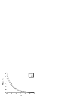
Figure 3: Temperature decay of the persistent current’s amplitudes in the $k=2,3$ and $4$ parafermion FQH states. The zero temperature amplitudes in these units are $\nu_{k}/2$.

References

• [1] N. Read and E. Rezayi, Phys. Rev. B 59, 8084 (1998).
• [2] W. Pan et al., Phys. Rev. Lett. 83, 3530 (1999).
• [3] J. FrΓΆhlich, U. M. Studer and E. Thiran, J. Stat. Phys.Β 86, 821 (1997).
• [4] A.B. Zamolodchikov and V.A. Fateev, Sov. Phys. JETP 62 (1985) 215, Nucl. Phys. B 280, 644 (1987) .
• [5] A. Cappelli, L. Georgiev and I. Todorov, Nucl. Phys. B 599, 499 (2001).
• [6] J. Fuchs, A.N. Schellekens and C. Schweigert, Nucl. Phys.Β B 461, 39 (1996).
• [7] P.Di Francesco, P. Mathieu and D. SΓ©nΓ©chal, Conformal Field Theory, Springer–Verlag, New York (1997).
• [8] J.K. Slingerland, F.A. Bais, Nucl. Phys.Β B 612, 229 (2001).
• [9] A. Cappelli and G.R. Zemba, Nucl. Phys.Β B 490, 595 (1997).
• [10] L. Georgiev, Phys. Rev.Β B 69, 085305 (2004).