hep-th/0402149

We present new self-gravitating solutions in five dimensions that describe circular strings, i.e., rings, electrically coupled to a two-form potential (as e.g., fundamental strings do), or to a dual magnetic one-form. The rings are prevented from collapsing by rotation, and they create a field analogous to a dipole, with no net charge measured at infinity. They can have a regular horizon, and we show that this implies the existence of an infinite number of black rings, labeled by a continuous parameter, with the same mass and angular momentum as neutral black rings and black holes. We also discuss the solution for a rotating loop of fundamental string. We show how more general rings arise from intersections of branes with a regular horizon (even at extremality), closely related to the configurations that yield the four-dimensional black hole with four charges. We reproduce the Bekenstein-Hawking entropy of a large extremal ring through a microscopic calculation. Finally, we discuss some qualitative ideas for a microscopic understanding of neutral and dipole black rings.

1 Introduction

Take a neutral black string in five dimensions, constructed as the direct product of the Schwarzschild solution and a line, so the geometry of the horizon is ${\bf R}\times S^{2}$. Imagine bending this string to form a circle, so the topology is now $S^{1}\times S^{2}$. In principle this circular string tends to contract, decreasing the radius of the $S^{1}$, due to its tension and gravitational self-attraction, but we can make the string rotate along the $S^{1}$ and balance these forces against the centrifugal repulsion. Then we end up with a neutral rotating black ring. Ref. [1] obtained it as an explicit solution of five-dimensional vacuum General Relativity.

This heuristic construction was first suggested surprisingly long ago in [2], but several of the most important features of the neutral black ring could hardly have been anticipated without the explicit solution. For fixed mass, the spin of a five-dimensional rotating black hole of spherical topology is bounded above [2], whereas the spin of the black ring is bounded below. But the ranges of existence of both sorts of objects overlap, and where they do, one actually finds two black rings, in addition to the black hole, all with the same mass and spin. This triplicity of solutions implies the non-uniqueness of five-dimensional black holes, and can be regarded as a sort of hair, even if it makes a rather thin wig.

A string can naturally couple to a two-form potential $B_{\mu\nu}$, and be an electric source for it, a familiar example being the fundamental string. Alternatively, its electric-magnetic dual in five dimensions would be a string magnetically charged under a one-form potential $A_{\mu}$. Take one such string and bend it into circular shape, balancing it again by appropriately spinning the ring. This configuration will have a non-trivial gauge field, but now the net charge will be zero. Actually, as we shall ellaborate shortly, it is appropriate to view it as a dipole, with zero net charge but with a non-vanishing local distribution of charge. So we may refer to the rotating circular strings as rotating dipole rings. These were conjectured to exist in ref. [3, 4, 5], and they are the subject of this paper.

The dipole field allows black rings to sport much thicker hair, and indeed it realizes a more drastic infinite non-uniqueness: the only conserved asymptotic charges of these rings are their mass and spin, but they support a gauge field labeled by parameters within a continuous range of values. This possibility was first anticipated in [4], and it will be realized below.

Since these solutions appear quite naturally in the supergravity description of string/M-theory at low energies, they give us a new perspective on the role of black rings within string theory, in a guise different from the one studied in [5]. We begin to explore it in this paper, and in particular provide the first precise microscopic calculation of the entropy of a black ring.

The structure of the paper is the following: Since the study of the solutions is somewhat technical, before plunging into the details we introduce, in the next section, the basic concepts and describe, in a graphical manner, the main features of dipole rings. In section 3, after a short description of the neutral rotating ring, we give the explicit form of the dipole solutions and compute their properties. In section 4 we address the issues raised by the solution that describes a rotating loop of fundamental string, and discuss qualitatively some features of dipole rings from a microscopic string viewpoint. In section 5 we explain how black rings appear in triple intersections of branes, with the rotation arising from momentum running along the intersection. We also reproduce the Bekenstein-Hawking entropy of the extremal black ring, to next-to-leading order at large radius, via a statistical-mechanical counting of string states. We conclude in section 6 with a discussion of the results and some qualitative considerations towards a broader microscopic view of black rings. The appendix shows how the Myers-Perry (MP) black hole [2] is recovered from the solutions in section 3.

2 Setup and summary of properties

We construct dipole ring solutions for a number of theories, the simplest of which are the five-dimensional Einstein-Maxwell-dilaton theories

$$I=\frac{1}{16\pi G}\int d^{5}x\sqrt{-g}\left(R-\frac{1}{2}(\partial\phi)^{2}-\frac{1}{4}e^{-\alpha\phi}F^{2}\right)\,.$$ (2.1)

The conventional Einstein-Maxwell theory is recovered when the dilaton decouples, i.e., $\alpha=0$. One often considers the addition of a Chern-Simons term to this theory, as required by minimal supergravity in five dimensions. It turns out that the Chern-Simons term is of no consequence to the solutions in this paper, and therefore the dipole rings with $\alpha=0$ are also solutions of minimal five-dimensional supergravity. Then the uniqueness theorem of supersymmetric black holes in this theory [4] directly implies that none of the black rings of the non-dilatonic theory can be a supersymmetric solution.

A ring is a circular string, and in the five-dimensional theories of (2.1), strings act as line sources of a magnetic field, i.e., they can be thought of as linear distributions of magnetic monopoles. So the field of a magnetic black ring, outside the horizon, can be described as being produced by a circular configuration of magnetic monopoles. It is important to realize that, even if there is a local distribution of charge, the total magnetic charge is zero [7]. The reason is that, in order to compute the magnetic charge in five dimensions, one has to specify a two-sphere that encloses a point of the string, and a vector tangent to the string. Since this vector changes orientation halfway around the ring, the total charge on the ring is zero. This can also be seen as the fact that on a 4D slice that cuts the ring at diametrically opposite points, one finds opposite magnetic charges. So the ring is analogous to a dipole.

We will also consider the electric dual of these solutions. The transformation

$$\tilde{\phi}=-\phi,\qquad H=e^{-\alpha\phi}\ast F\,,$$ (2.2)

where $H=dB$ is a three-form field strength, maps the theory (2.1) to

$$I=\frac{1}{16\pi G}\int d^{5}x\sqrt{-g}\left(R-\frac{1}{2}(\partial\tilde{\phi})^{2}-\frac{1}{12}e^{-\alpha\tilde{\phi}}H^{2}\right)\,.$$ (2.3)

It will be convenient to express the dilaton coupling as

$$\alpha^{2}=\frac{4}{N}-\frac{4}{3}\,,\qquad 0<N\leq 3\,,$$ (2.4)

since the values $N=1,2,3$ are of particular relevance to string and M-theory. In these cases the solution can be regarded as an $N$-fold intersection of branes, which typically wrap an internal space (see e.g., [6]). $N=3$ yields the non-dilatonic theory, but another case of particular interest is $N=1$, since then the action (2.3) can be interpreted as the NS sector of low energy string theory (in Einstein frame), and it contains the fundamental string as a solution. The dilaton $\sigma$ of string theory is in this case $\sigma=\sqrt{\frac{3}{8}}\>\tilde{\phi}$ and the string metric $g^{(s)}_{\mu\nu}=e^{\sqrt{\frac{2}{3}}\>\tilde{\phi}}g_{\mu\nu}$. Via dualities the solution is related as well to other single-brane configurations.

One can define a “local charge” for the string solutions of (2.3) as

$${\cal Q}=\frac{1}{4\pi}\int_{S^{2}}e^{-\alpha\tilde{\phi}}\ast H\,,$$ (2.5)

where the $S^{2}$ encloses a point along the string, and give it a sign according to a choice of orientation along the string. To see the meaning of this charge, consider first the case of a straight fundamental string. This is infinitely long, but it can be made finite by requiring the spatial direction parallel to the string to form a compact circle. The string has a topological winding number that is proportional to the local charge (2.5),

$$n=\frac{\pi\alpha^{\prime}}{2G}{\cal Q}\,,$$ (2.6)

and this is a conserved quantity that measures the number of times that the string goes around the circle before closing in on itself, or alternatively the number of closed strings singly-wound on the circle. In general, the winding $n\propto{\cal Q}$ can also be defined, with a different proportionality factor, for dual brane realizations of the $N=1$ solution, while for $N=2,3$ obtained from brane intersections, the winding of the “effective string” at the intersection is proportional to ${\cal Q}^{N}$.

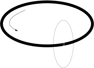
Figure 1: The non-topological winding number $n$ of the ring is proportional to the local charge ${\cal Q}$ measured from the electric flux of $H$ across an $S^{2}$ that encloses a section of the string. An azimuthal angle has been suppressed in the picture, so the $S^{2}$ is represented as a circle.

Consider now a circular string loop in asymptotically flat spacetime (no compact circle). We can also regard it as a closed string, but now it does not wrap any topologically non-trivial cycle. Instead, it winds around a contractible circle, but we can still define the local charge ${\cal Q}$ (2.5) (see fig. 1), and $n$ as in (2.6). Now $n$ is not topological, but it still measures the number of windings of the string around the circle. So even in the case where the charge is not a conserved quantity, it has a clear physical meaning and it provides the most natural characterization of the source of the dipole field.

Dipole rings are therefore specified by the three physical parameters $(M,J,{\cal Q})$. The third parameter, which is independent of the other two, is not a conserved charge, and is classically a continuous parameter. So, as we will see in detail, it implies infinite non-uniqueness in five dimensions. Upon quantization in string theory these parameters become discrete, and there will be a finite but still very large number of states with the same mass and spin.

We are now ready to summarize the features of the dipole rings that follow from the detailed analysis of the next section. We can adequately fix the overall scale of the solutions by fixing their mass $M$. Then the solutions are characterized by reduced dimensionless magnitudes, obtained by dividing out an appropriate power of $M$, or of $GM$ (which has dimension (length)²), e.g., we define a dimensionless “reduced spin” variable $j$, conveniently normalized as

$$j^{2}\equiv\frac{27\pi}{32G}\frac{J^{2}}{M^{3}}\,,$$ (2.7)

($j^{2}$ is often a more convenient variable than $j$), as well as a reduced area of the horizon,

$${a_{H}}\equiv\frac{3}{16}\sqrt{\frac{3}{\pi}}\frac{{\cal A}_{H}}{(GM)^{3/2}}\,,$$ (2.8)

and a reduced local charge,

$$q\equiv\frac{{\cal Q}}{\sqrt{GM}}\,.$$ (2.9)

The properties of the neutral solutions ($q=0$) found in [1] are summarized in the plot of $a_{H}$ vs $j^{2}$ in figure 2. The explicit analytical form of the curves is given below in (3.8), (3.9). The non-uniqueness in $27/32\leq j^{2}<1$ is clear from the figure. Note we have normalized ${a_{H}}$ so that its maximum value for a neutral ring is $1$.

Figure 2: Plot of horizon area vs (spin)², for given mass, for the neutral rotating black ring (solid) and black hole (dotted). The reduced variables $j^{2}$ and $a_{H}$ are defined in (2.7), (2.8). There are two branches of black rings, which branch off from the cusp at $(j^{2},a_{H})=(27/32,1)$, and which are dubbed “large” and “small” according to their area. For spins in the range $27/32\leq j^{2}<1$ the black rings in the two branches coexist with a black hole of the same mass and spin, implying three-fold non-uniqueness. Other interesting features are: The black hole at $j^{2}=27/32$, i.e., with the same mass and spin as the minimally spinning ring, has ${a_{H}}=\sqrt{5}/2$. At $j^{2}={a_{H}}^{2}=8/9$ the curves intersect and we find a black hole and a (large) black ring both with the same mass, spin and area. The limiting solution at $(j^{2},a_{H})=(1,0)$ is a naked singularity. Fastly spinning black rings, $j^{2}\to\infty$, become thinner and their area decreases as ${a_{H}}\sim 1/(j\sqrt{2})$.

For the dipole-charged solutions we focus on the values of the dilaton coupling most relevant to string theory, namely $N=1,2,3$ in (2.4). The space of solutions is a two-dimensional surface in the space $(j,q,{a_{H}})$. Rather than a 3D plot of this surface, a clearer representation is obtained plotting several sections of it at constant $q$ as curves in the plane $(j^{2},{a_{H}})$. These are depicted in fig. 3.

Figure 3: $a_{H}$ vs $j^{2}$, for different values of $q$, for dipole rings with dilaton coupling $\alpha=2\sqrt{2/3},\sqrt{2/3},0$ ($N=1,2,3$). $q$ varies continuously, but we have plotted the curves for only a few representative values, with $q$ increasing in the direction of the arrow: shorter dashing corresponds to larger $q$, and the solid curves correspond to the neutral ring ($q=0$). For any fixed $j$, i.e., fixed mass and spin, such that $j^{2}>27/32$, there are always rings with $q$ in a continuous range of values, implying continuous non-uniqueness. Observe also that for fixed $q\neq 0$, $j$ is bounded above and below so the range of allowed spins is finite, and becomes narrower as $q$ grows. When $q$ reaches its maximum value the curves degenerate to a point, which is at $(j^{2},a_{H})=(1,0)$, $(.95,0)$, $(.93,.37)$ for $N=1,2,3$ resp. (see fig. 5 for the maximum values of $q$). For $N=3$, the endpoints of the curves lie on the thick grey line, which corresponds to extremal dipole rings of finite horizon area.

It becomes apparent that if we fix the mass and the angular momentum, with $j^{2}>27/32$, there exist black ring solutions with $q$ taking values over a continuous finite interval. Black hole uniqueness is then violated by a continuous parameter, and therefore in an infinite manner.

There are other features common to all values of $N$. Like in the neutral case, for fixed $q$ there are two branches of black rings, one of them having larger area than the other, and in the range where they coexist we find two black rings with the same mass, spin and local charge. The two branches join at the slowest spinning ring with the given $q$, and this ring always has larger spin and smaller area than the minimally spinning neutral ring. The smaller area is easy to understand if we recall that adding charge to a black hole while keeping its mass fixed typically reduces its area. The larger spin is needed in order to counterbalance the attraction between diametrically opposite sections of the ring, which as we saw can be regarded as oppositely charged.

In contrast to the neutral case, where the spin of large rings is unbounded, the spin of large dipole rings has an upper bound. The solutions which saturate the bound are extremal (but non-supersymmetric) rings, meaning that the outer and inner horizons come to coincide. A qualitative explanation for this upper bound will be provided in section 4. Of these extremal solutions, the only ones that have non-zero area are the non-dilatonic extremal rings, i.e., $N=3$. This was expected, since the extremal limit of the straight strings in five dimensions results in non-zero area only when $N=3$. For $N>1$ the small ring branch also has an extremal limit, which corresponds to maximum $j$ in that branch, and which have non-zero area only if $N=3$. In the $N=3$ plot in fig. 3 we draw the area of the extremal solutions as a thick grey line, but one should bear in mind that $q$ is not constant along this curve, i.e., the relation between ${\cal Q}$ and $M$ at extremality is not fixed but changes with $J$. For $N=1$ the branch of small rings terminates at a singular solution before the extremal limit is reached.

In section 5 we exhibit rotating dipole ring solutions of string and M-theory at low energies, that arise from the intersection of three kinds of branes with different dipole charges, e.g., D2, D6 and NS5 brane charges, and which reduce to the cases $N=1,2,3$ above by having equal numbers of one, two, or three of the component branes, and no branes of the remaining components. Their features are qualitatively the same as described above, according to the number of component branes that are present.

As we will see, many of the qualitative properties of large rings are similar to those of their straight string limits. Since we often have a microscopic stringy picture of the latter, this allows us to get at least a qualitative microscopic picture of large rings, and understand some of the features described above, as we will explain in sections 4 and 5. The small ring branch is more intriguing, but we will be able to make some reasonable suggestions about its meaning in section 6.

We finish this section mentioning how earlier ring solutions are related to the ones in this paper. The first example in this class that we are aware of is the construction of a self-gravitating static loop of string described in [7]. This is a static, extremal dipole ring with dilaton coupling $N=1$. It does not have a regular horizon, and in the absence of rotation or any external field, it contains a conical singularity disk. Ref. [3] generalized it to static extremal dipole rings with arbitrary dilaton coupling $\alpha$, and also to static extremal rings from triple intersections of branes. All these solutions are recovered (in different coordinates) from the solutions in this paper by setting the rotation to zero and taking the extremal limit. When $N=3$ they have a regular degenerate horizon, but they still contain conical singularities (if no fluxbrane is added). Refs. [8, 5] constructed charged black rings, but these have a net charge (besides dipole charges, not independent of the net charges), and are therefore different from the ones in this paper.

We turn now to the explicit form of the solutions, and to explain how the features we have described are obtained.

3 Dipole black ring solutions

The neutral rotating black ring was obtained in [1] from the Kaluza-Klein C-metric solutions in [9] via a double Wick rotation of coordinates and analytic continuation of parameters. All the new solutions in this paper are similarly obtained from the generalized C-metrics found in [10]. It turns out that the coordinates and parameters in which these new black rings are expressed more simply are slightly different from those previously used for black rings in [1, 5], so we need to begin with a brief description of the neutral solution in these new coordinates. They share the feature with the coordinates in [11, 5] that the cubic functions involved take a factorized form and allow for easier analytic evaluation than in the original form in ref. [1]. This allows us to provide some new analytical results.

3.1 Neutral ring

The metric is

$$ds^{2} = -\frac{F(y)}{F(x)}\left(dt+C(\nu,\lambda)\>R\>\frac{1+y}{F(y)}\>d\psi\right)^{2}$$ (3.1)

$$+\frac{R^{2}}{(x-y)^{2}}\>F(x)\left[-\frac{G(y)}{F(y)}d\psi^{2}-\frac{dy^{2}}{G(y)}+\frac{dx^{2}}{G(x)}+\frac{G(x)}{F(x)}d\varphi^{2}\right]\,,$$

where

$$F(\xi)=1+\lambda\xi,\qquad G(\xi)=(1-\xi^{2})(1+\nu\xi)\,,$$ (3.2)

and

$$C(\nu,\lambda)=\sqrt{\lambda(\lambda-\nu)\frac{1+\lambda}{1-\lambda}}\,.$$ (3.3)

The coordinates $x$ and $y$ vary within the ranges

$$-1\leq x\leq 1\,,\qquad-\infty<y\leq-1\,,$$ (3.4)

and the dimensionless parameters $\lambda$ and $\nu$ within

$$0<\nu\leq\lambda<1\,.$$ (3.5)

$R$ has dimensions of length, and for thin large rings it corresponds roughly to the radius of the ring circle [5]. In order to avoid conical singularities at $y=-1$ and $x=-1$ the angular variables must be identified with periodicity

$$\Delta\psi=\Delta\varphi=2\pi\frac{\sqrt{1-\lambda}}{1-\nu}\,.$$ (3.6)

To avoid also a conical singularity at $x=+1$ we take the two parameters $\lambda$, $\nu$, to be related as

$$\lambda=\frac{2\nu}{1+\nu^{2}}\,.$$ (3.7)

With these choices, the solution has a regular horizon of topology $S^{1}\times S^{2}$ at $y=-1/\nu$, an ergosurface of the same topology at $y=-1/\lambda$, and an inner spacelike singularity at $y=-\infty$. Asymptotic spatial infinity is reached as $x\to y\to-1$. The coordinate system is illustrated in fig. 4.

Figure 4: Coordinate system for black ring metrics (adapted from [12]). The diagram sketches a section at constant $t$ and $\varphi$. Surfaces of constant $y$ are ring-shaped, while $x$ is a polar coordinate on the $S^{2}$ (roughly $x\sim\cos\theta$). $x=\pm 1$ and $y=-1$ are fixed-point sets (i.e., axes) of $\partial_{\varphi}$ and $\partial_{\psi}$, resp. Infinity lies at $x=y=-1$.

A static ring solution, which necessarily contains a conical singularity, is obtained when instead of (3.7) we set $\lambda=\nu$ [12]. The spherical black hole of Myers and Perry with rotation in a single plane can also be obtained from (3.1), but in the coordinates in (3.1) this case is much subtler than when using the forms of the metric employed in [1, 5]. The appropriate limiting procedure is described in the appendix. When $\nu\to 1$ the solution becomes singular and the horizon is replaced by a naked singularity.

The mass, spin, and other physical parameters of the neutral black ring can be readily recovered as the neutral limit $\mu\to 0$ of the expressions for the dipole ring, eqs. (3.23)-(3.27) below, so we will not present them here. Note that for a black ring at equilibrium, i.e., satisfying (3.6) and (3.7), there is only one independent dimensionless parameter, so the reduced area and spin, (2.7), (2.8), must be related. ${a_{H}}$ and $j$ can be computed from the expressions for $M$, $J$ and ${\cal A}_{H}$, and the analytic relation between them is, in parametric form,

$${a_{H}}=2\sqrt{\nu(1-\nu)}\,,\qquad j^{2}=\frac{(1+\nu)^{3}}{8\nu}\qquad\mathrm{(black\>ring)}\,,$$ (3.8)

with $0<\nu\leq 1$. On the other hand, for the spherical black hole,

$${a_{H}}=2\sqrt{2(1-j^{2})}\qquad\mathrm{(black\>hole)}\,.$$ (3.9)

These curves were plotted and discussed in figure 2.

Finally, in order to see how we recover a boosted straight black string in the limit where the radius of the ring circle grows very large, define

$$r_{0}=\nu R\,,\qquad\cosh^{2}\sigma=\frac{\lambda}{\nu}\,,$$ (3.10)

and

$$r=-\frac{R}{y}\,,\quad\cos\theta=x\,,\quad w=R\psi$$ (3.11)

and take the limit $R\to\infty$, $\lambda,\nu\to 0$, keeping $r_{0},\sigma$ and $r,\theta,w$ finite. Then we obtain the metric for a boosted black string

$$ds^{2}=-\hat{f}\left(dt-\frac{r_{0}\sinh\sigma\cosh\sigma}{r\hat{f}}\>dw\right)^{2}+\frac{f}{\hat{f}}\>dw^{2}+\frac{dr^{2}}{f}+r^{2}d\Omega_{(2)}^{2}$$ (3.12)

where

$$f=1-\frac{r_{0}}{r}\,,\qquad\hat{f}=1-\frac{r_{0}\cosh^{2}\sigma}{r}\,.$$ (3.13)

The value of the boost obtained from the limit of rings at equilibrium is, from (3.7) and (3.10), $|\sinh\sigma|=1$, and this was shown in [5] to make the ADM pressure $T_{ww}=0$ (see eq. (3.2) below, with $\gamma=0$) .

Even if $\lambda$ and $\nu$ do not directly correspond to physical quantities (whereas $j^{2}$ and ${a_{H}}$ do), eq. (3.10) allows to find an approximate meaning for them, which becomes more accurate for thin rings. For large but finite $R$, the parameter $\nu\simeq r_{0}/R$ measures the ratio between the radius of the $S^{2}$ at the horizon and the radius of the ring. So smaller values of $\nu$ correspond to thinner rings. Also, $\lambda/\nu$ is a measure of the speed of rotation of the ring. More precisely, $\sqrt{1-(\nu/\lambda)}$ can be approximately identified with the local boost velocity $\tanh\sigma$, which for rings in equilibrium, (3.7), is $\sqrt{(1-\nu^{2})/2}$.

3.2 Dipole rings

The dipole black ring solutions contain a new parameter $\mu$, related to the local charge ${\cal Q}$ of the ring. For arbitrary dilaton coupling $\alpha$, expressed in terms of $N$ as in (2.4), the geometry of the solutions is

$$ds^{2} = -\frac{F(y)}{F(x)}\left(\frac{H(x)}{H(y)}\right)^{N/3}\left(dt+C(\nu,\lambda)\>R\>\frac{1+y}{F(y)}\>d\psi\right)^{2}$$

$$+\frac{R^{2}}{(x-y)^{2}}\>F(x)\left(H(x)H(y)^{2}\right)^{N/3}\left[-\frac{G(y)}{F(y)H(y)^{N}}d\psi^{2}-\frac{dy^{2}}{G(y)}+\frac{dx^{2}}{G(x)}+\frac{G(x)}{F(x)H(x)^{N}}d\varphi^{2}\right]\,.$$

The functions $F$ and $G$ are like in (3.2), and

$$H(\xi)=1-\mu\xi\,.$$ (3.15)

If we consider the magnetic solutions of the Einstein-Maxwell-dilaton theory (2.3) then the gauge potential is

$$A_{\varphi}=C(\nu,-\mu)\>\sqrt{N}\>R\>\frac{1+x}{H(x)}+k_{1}\,,$$ (3.16)

(the constant $k_{1}$ moves Dirac strings around) and the dilaton

$$e^{-\phi}=\left(\frac{H(x)}{H(y)}\right)^{N\alpha/2}\,.$$ (3.17)

$C(\nu,-\mu)$ is like in (3.3) but with $\lambda\to-\mu$. Since this field is purely magnetic, it makes no contribution to the Chern-Simons term required by five-dimensional supergravity, and so the solution belongs in this theory as well.

For the electric solutions of (2.3), the metric is the same as above, the dilaton $\tilde{\phi}=-\phi$, and the two-form potential

$$B_{t\psi}=C(\nu,-\mu)\>\sqrt{N}\>R\>\frac{1+y}{H(y)}+k_{2}\,.$$ (3.18)

The constant $k_{2}$ may be chosen at convenience, e.g., to make $B_{t\psi}$ vanish at $y=-1/\nu$.

The parameters $\lambda$ and $\nu$ vary in the same ranges as in the neutral case (3.5), while

$$0\leq\mu<1\,.$$ (3.19)

When $\mu=0$ we recover the neutral solution (3.1).

Most of the features of the solutions are analyzed in the same manner as for the neutral black ring, so we refer to the previous section and earlier papers [1], [5] for more details. The coordinate $x$ varies in $[-1,1]$. Initially we take $y\in(-\infty,-1]$, but we will shortly see that this can be extended across $|y|=\infty$ to the range $(1/\mu,+\infty)$. The possible conical singularities at the axes extending to infinity, $x=-1$ and $y=-1$, are avoided by setting

$$\Delta\psi=\Delta\varphi=4\pi\frac{H(-1)^{N/2}\sqrt{F(-1)}}{|G^{\prime}(-1)|}=2\pi\frac{(1+\mu)^{N/2}\sqrt{1-\lambda}}{1-\nu}\,.$$ (3.20)

The balance between forces in the ring will be achieved when, in addition, there are no conical singularities at $x=+1$. This requires that

$$\Delta\varphi=4\pi\frac{H(+1)^{N/2}\sqrt{F(+1)}}{|G^{\prime}(+1)|}\,,$$ (3.21)

which can be satisfied simultaneously with (3.20) only if

$$\frac{1-\lambda}{1+\lambda}\left(\frac{1+\mu}{1-\mu}\right)^{N}=\left(\frac{1-\nu}{1+\nu}\right)^{2}\,.$$ (3.22)

In the neutral case $\mu=0$ this equation is solved by (3.7).

Under these conditions, it is easy to see that the solution has a regular outer horizon of topology $S^{1}\times S^{2}$ at $y=-1/\nu$. In addition, there is an inner horizon at $y=-\infty$. The metric can be continued beyond this horizon (as in e.g., [1]) to positive values $1/\mu<y<\infty$, until $y=1/\mu$ is hit from above, which is a curvature singularity. The two horizons coincide when $\nu=0$, which defines the extremal limit, and $\nu$ can be regarded as a non-extremality parameter. In general, a ring-shaped ergosurface is present at $y=-1/\lambda$.

The calculation of the mass, angular momentum, horizon area, temperature (from surface gravity) and angular velocity at the (outer) horizon is straightforward, and one finds

$$M=\frac{3\pi R^{2}}{4G}\frac{(1+\mu)^{N}}{1-\nu}\left(\lambda+\frac{N}{3}\frac{\mu(1-\lambda)}{1+\mu}\right)\,,$$ (3.23)

$$J=\frac{\pi R^{3}}{2G}\frac{(1+\mu)^{3N/2}\sqrt{\lambda(\lambda-\nu)(1+\lambda)}}{(1-\nu)^{2}}\,,$$ (3.24)

$${{\cal A}_{H}}=8\pi^{2}R^{3}\frac{(1+\mu)^{N}\nu^{(3-N)/2}(\mu+\nu)^{N/2}\sqrt{\lambda(1-\lambda^{2})}}{(1-\nu)^{2}(1+\nu)}\,,$$ (3.25)

$$T=\frac{1}{4\pi R}\frac{\nu^{(N-1)/2}(1+\nu)}{(\mu+\nu)^{N/2}}\sqrt{\frac{1-\lambda}{\lambda(1+\lambda)}}\,,$$ (3.26)

$$\Omega=\frac{1}{R}\frac{1}{(1+\mu)^{N/2}}\sqrt{\frac{\lambda-\nu}{\lambda(1+\lambda)}}\,.\\$$ (3.27)

We can also compute the local charge ${\cal Q}$ defined in (2.5). The integral is taken over an $S^{2}$ parametrized by $(x,\varphi)$, at constant $t$, $\psi$ and $y\in(-1/\nu,-1)$, see fig. 4. Then

$${\cal Q}=R\sqrt{N}\frac{(1+\mu)^{(N-1)/2}\sqrt{\mu(\mu+\nu)(1-\lambda)}}{(1-\nu)\sqrt{1-\mu}}\,.$$ (3.28)

In addition, we define the potential $\Phi$ from the difference between the values of $B$ at infinity and at the horizon,

$$\Phi=\frac{\pi}{2G}\left[B_{t\tilde{\psi}}(x=y=-1)-B_{t\tilde{\psi}}(y=-1/\nu)\right],$$ (3.29)

where $\tilde{\psi}=(2\pi/\Delta\psi)\psi$ is the canonically normalized angular variable, and the factor $\pi/2G$ is introduced simply for convenience. Then

$$\Phi=\frac{\pi R}{2G}\sqrt{N}\frac{(1+\mu)^{(N-1)/2}\sqrt{\mu(1-\mu)(1-\lambda)}}{\sqrt{\mu+\nu}}\,.$$ (3.30)

A straightforward calculation using these results shows that the black ring satisfies a Smarr relation

$$M=\frac{3}{2}\left(\frac{1}{4G}{{\cal A}_{H}}T+\Omega J\right)+\frac{1}{2}{\cal Q}\Phi\,.$$ (3.31)

The first law

$$dM=\frac{1}{4G}Td{{\cal A}_{H}}+\Omega dJ+\Phi d{\cal Q}\,,$$ (3.32)

can also be, somewhat laboriously, verified explicitly. The numerical coefficients in (3.31) and (3.32) are consistent with the homogeneity properties of $M$ as a function of scaling dimension 2, of the variables ${\cal A}_{H}$, $J$, ${\cal Q}$ with scaling dimensions 3, 3, 1, resp.

The horizon area of dilatonic rings vanishes in the extremal limit $\nu\to 0$. These are nakedly singular solutions. Only in the non-dilatonic case $N=3$ does the area remain finite as $\nu\to 0$, and the solution has a regular degenerate horizon. The mass $M$ and local charge ${\cal Q}$ are not any simply related in the extremal limit, and for finite values of $R$, the extremal solutions are not supersymmetric.

The main properties of dipole rings are summarized in fig. 3. In order to produce these plots, we first solve eq. (3.22) for $\lambda$ as a function of $\nu$ and $\mu$. Using (3.23)-(3.28), we compute the reduced local charge $q$, spin $j$, and area $a_{H}$, as functions of $\mu$ and $\nu$, and then we invert to find $\mu$ as a function of $q$ and $\nu$. The inverted function can be seen to involve more than one branch for $N>1$. All of this can be done fully analitically for $N=1,2,3$, but the expressions are exceedingly long and only simplify in the extremal limit. So we proceed using a symbolic manipulation computer program. Eventually we obtain $a_{H}$ and $j^{2}$ as functions of $\nu$ and $q$, which allows us to plot the curves for fixed $q$, varying $0\leq\nu\leq 1$. We refer to section 2 for a discussion.

The limit where the ring becomes a straight string allows us again to get a feeling for other properties of the solutions. In addition to taking $\lambda,\nu\to 0$, $R\to\infty$ with (3.10) and (3.11) finite, we also take $\mu\to 0$ and keep finite

$$\mu R=r_{0}\sinh^{2}\gamma\,,$$ (3.33)

where $\gamma$ gives a convenient parametrization of the charge in this limit. Then the limiting solution is

$$ds^{2}=-\frac{\hat{f}}{h^{N/3}}\left(dt-\frac{r_{0}\sinh\sigma\cosh\sigma}{r\hat{f}}\>dw\right)^{2}+\frac{f}{h^{N/3}\hat{f}}\>dw^{2}+h^{2N/3}\left(\frac{dr^{2}}{f}+r^{2}d\Omega_{(2)}^{2}\right)\,,$$ (3.34)

$$A_{\varphi}=\sqrt{N}r_{0}\sinh\gamma\cosh\gamma(\cos\theta+1)\,,\qquad e^{\phi}=h^{N\alpha/2}\,,$$ (3.35)

for the magnetic solution, and

$$B_{tw}=\sqrt{N}r_{0}\sinh\gamma\cosh\gamma(h^{-1}-1)\,,\qquad e^{\tilde{\phi}}=h^{-N\alpha/2}\,,$$ (3.36)

for the electric one, where $f$ and $\hat{f}$ were defined in (3.13), and

$$h=1+\frac{r_{0}\sinh^{2}\gamma}{r}\,.$$ (3.37)

These are five-dimensional charged strings with a momentum wave. When $N=3$ and $\gamma=\sigma$, the reduction along $w$ to four dimensions yields the Reissner-Nordstrom black hole.

While the straight string (3.34) solves the field equations for arbitrary values of $\sigma$ and $\gamma$, the strings that are obtained as a limit of rings that satisfy the equilibrium condition (3.22) must, from this condition, be such that

$$\sinh^{2}\sigma=1+N\sinh^{2}\gamma\,.$$ (3.38)

Note that when $\gamma\neq 0$ the boost has to be larger than in the neutral case $\gamma=0$. This is easily interpreted: sections of the ring at diametrically opposite ends, $\psi$ and $\psi+\pi$, have opposite orientation and therefore they attract each other via the $H_{\mu\nu\rho}$ field. Then a larger centrifugal repulsion is needed in order to achieve equilibrium, and the effect persists even at very large ring radii.

The ADM stress-energy tensor of the string (3.34) is

$$T_{tt} = \frac{r_{0}}{4G}(1+\cosh^{2}\sigma+N\sinh^{2}\gamma)\,,$$

$$T_{ww} = \frac{r_{0}}{4G}\left(\sinh^{2}\sigma-1-N\sinh^{2}\gamma\right)\,,$$ (3.39)

$$T_{tw} = \frac{r_{0}}{4G}\sinh\sigma\cosh\sigma\,.$$

We observe that, as was the case for the neutral ring and the charged rings of [5], the pressure $T_{ww}$ of the limiting string vanishes when the equilibrium condition (3.38) is enforced. The restrictions on the parameters of the strings that result as a limit of balanced rings, such as eq. (3.38), are in general poorly understood (see also [5]), and although it is clear that they are the result of an equilibrium of forces, it would be interesting to understand them in more detail. At any rate, in the limit we still recover the identification

$$\frac{M}{2\pi R}\to T_{tt}\,,\qquad\frac{J}{2\pi R^{2}}\to T_{tw}\,,$$ (3.40)

while ${\cal Q}\to\sqrt{N}r_{0}\sinh\gamma\cosh\gamma$ is identified as the black string charge under the $H$ field.

3.3 Extremal rings

The extremal solutions are defined as the limiting case where the outer and inner horizons coincide. For the dilatonic solutions the horizon turns into a null singularity, whereas the non-dilatonic extremal ring has a regular degenerate horizon. Typically, the extremal limit yields solutions where the spin and/or the charge reach a maximum value. In the present case, if we fix the mass and the spin, with $j^{2}>1$, then there is always a maximum value of ${\cal Q}$ which is saturated precisely in the extremal limit $\nu\to 0$. For $27/32<j^{2}<1$ the situation is more complicated and depends on the dilaton coupling, as can be seen in fig. 3. On the other hand, if we fix the local charge and the mass, i.e., fix $q$, the spin reaches an absolute maximum at an extremal solution along the large ring branch. There is also a local maximum along the small ring branch, but this solution is extremal only for $N>1$. For $N=1$ this local maximum is not an extremal solution. In this case the branch of small black rings with $q<q_{\rm max}=\sqrt{2/3\pi}$ terminates at $\nu=[1-(q/q_{\rm max})^{2}]/[1+(q/q_{\rm max})^{2}]$, i.e., before $\nu=0$, so these should not be interpreted as extremal solutions, except when $q\to q_{\rm max}$.

In the extremal limit the physical variables admit simple enough expressions in terms of the only dimensionless parameter that remains after imposing the equilibrium condition (3.22), and which we take to be $\mu$. Namely, for the extremal $N=1$ solution (for which the equilibrium condition becomes simply $\lambda=\mu$) we find

$$j^{2}=\frac{27(1+\mu)^{4}}{16\mu(2+\mu)^{3}}\,,\qquad{q}=\sqrt{\frac{2\mu}{\pi(2+\mu)}}\,,\qquad{a_{H}}=0\,.$$ (3.41)

For $N=2$:

$$j^{2}=\frac{27(1+\mu)^{5}}{4\mu(4+\mu+\mu^{2})^{3}}\,,\qquad{q}=\sqrt{\frac{4\mu(1-\mu)}{\pi(4+\mu+\mu^{2})}}\,,\qquad{a_{H}}=0\,.$$ (3.42)

For $N=3$:

$$j^{2}=\frac{(1+\mu)^{6}(3+\mu^{2})^{2}}{128\mu(1+\mu^{2})^{3}}\,,\quad{q}=\sqrt{\frac{\mu(1-\mu)^{2}}{\pi(1+\mu^{2})}}\,,\quad{a_{H}}=\sqrt{\frac{\mu(1-\mu^{2})^{3}(3+\mu^{2})}{4(1+\mu^{2})^{3}}}\,.$$ (3.43)

Figure 5: (Spin)² vs local charge, for extremal rings of fixed mass. Although we only plot the cases of integer $N$, the curves for all $1<N\leq 3$ are qualitatively similar to $N=2,3$, while for $0<N<1$ there is no upper bound for $q$, and the curve asymptotes to $j^{2}=1$ as $q\to\infty$.

We plot $j^{2}$ vs $q$ in fig. 5. Observe the existence of a maximum value of $q$ in all three cases (it is also possible to see that if $N<1$ there is no such upper bound). We will interpret this feature from a microscopic viewpoint in the next section. For $N=2,3$, when $q$ is below this maximum value there exist two extremal ring solutions with the same mass and dipole charge, but different spin. These two rings are the extremal limits of solutions in the large and small ring branches that we mentioned above. Note the absence of a second $N=1$ extremal solution, for fixed $q$, in fig. 5.

In [3] it was observed that when the $N=3$ extremal static ring is balanced by a fluxbrane of appropriate strength, then the geometry near the horizon of the ring becomes exactly AdS${}_{3}\times S^{2}$. Ref. [5] conjectured that this might be the case as well when the ring is balanced not by a fluxbrane but by rotation, as in the present paper. However, closer examination reveals that this is not the case: for any finite value of $R$ the near-horizon extremal geometry is distorted away from AdS${}_{3}\times S^{2}$ by factors of the polar angle of the $S^{2}$.

4 Loop of fundamental string, and qualitative microscopics

The extremal ring solution is particularly simple when $N=1$. Since the local charge in this case can be regarded as fundamental string charge, it is expected to describe a rotating loop of fundamental string. However, this appears to raise a puzzle, since it is well known that in perturbative string theory it is impossible to have a closed string loop that rotates like a rigid wheel. The resolution is fairly simple, and can be understood more simply if we focus first on the similar situation posed by a straight string that carries linear momentum.

Refs. [13, 14] constructed solutions of low energy string theory with non-zero winding and momentum of the form

$$ds^{2}=-\frac{1}{h}du\>dv-(h^{-1}-1)|\dot{\mathbf{F}}|^{2}dv^{2}+2(h^{-1}-1)\dot{\mathbf{F}}\cdot d\mathbf{x}\>dv+d\mathbf{x}\cdot d\mathbf{x}$$ (4.44)

where $u,v$ are light-cone coordinates, $\mathbf{F}(v)$ parametrizes a curve in the $d-2$ transverse directions $\bf x$, and $h$ is a harmonic function

$$h=1+\frac{Q}{|\mathbf{x}-\mathbf{F}|^{d-4}}$$ (4.45)

(we will not need the dilaton and $H$ field for our argument) so the solution is singular at $\mathbf{x}=\mathbf{F}(v)$. $Q$ is proportional to the winding number of the string. It was shown in [14] that one can match these solutions to a fundamental string source, with a profile of momentum-carrying transverse oscillations given by $\mathbf{F}(v)$.

Now consider fundamental strings with small oscillation amplitudes, such that when we perform a coarse-grain average over their oscillation profiles we get $\langle\mathbf{F}\rangle\simeq 0$ and $\langle\dot{\mathbf{F}}\cdot\mathbf{x}\rangle\simeq 0$, but $\langle|\dot{\mathbf{F}}|^{2}\rangle\neq 0$. We shall not be too precise about how this averaging is performed, but one can suppose, along the lines of [15], that we choose not to resolve distances smaller than a typical amplitude, so we remain at $|\mathbf{x}|\gg|\mathbf{F}|$. The coarse-grained metric is then approximated by

$$ds^{2}=-\frac{1}{h}du\>dv+\frac{p}{|\mathbf{x}|^{d-4}h}dv^{2}+d\mathbf{x}\cdot d\mathbf{x}$$ (4.46)

with $h=1+Q/|\mathbf{x}|^{d-4}$ and $p=Q\langle|\dot{\mathbf{F}}|^{2}\rangle$, i.e., we can regard the strings as oscillating about a center-of-mass line at $\mathbf{x}=0$, and carrying a large, macroscopic total momentum density $Q\langle|\dot{\mathbf{F}}|^{2}\rangle$.

So, after averaging over strings with small oscillations, the effective solution (4.46) looks like a string with a longitudinal momentum wave. Since it is well known that relativistic fundamental strings cannot support longitudinal oscillations, the proper interpretation of (4.46) must be in terms of this averaging procedure. This interpretation is, for the purposes of this paper, basically the same as the microscopic proposal for the two- and three-charge black hole solutions in [15, 16, 17]. Following [16, 17], we may refer to (4.46) as the “naive” solution for a string carrying momentum, which is a coarse-grained average over the structure near the core of the “correct” metrics (4.44).

The extremal rings of this paper are now seen to be “naive” metrics, as (4.46). Indeed, the limit of infinite radius (3.34) for the $N=1$ extremal solutions is precisely the metric (4.46) in $d=5$ with $Q={\cal Q}$. So the rotating loop of string is an effective coarse-grained description of strings which oscillate about the ring, with amplitude much smaller than the ring radius, and the rotation is provided by the momentum circulating along the ring carried by these oscillations. One would also expect the existence of “correct” ring solutions, analogous to (4.44), where the momentum wave is resolved into transverse oscillations of the string, but due to the absence of supersymmetry it appears difficult to find these solutions analytically. It would also be interesting to construct the rotating loops of string, with oscillations, as classical solutions of perturbative string theory.

This picture allows us to get a qualitative microscopic understanding of some features of extremal dipole rings. Our main assumptions are that (a) extremal solutions correspond to strings with chiral oscillations, i.e., only left-movers (or only right-movers), and (b) that ${\cal Q}$ gives, through eq. (2.6), the number $n$ of strings wound in the loop (or alternatively, the number of windings of a single string $n$ times longer). Then we can see that there must be an upper bound on the spin for fixed ${\cal Q}$ and $M$, which is saturated in the extremal limit. For, if we fix $n$ and the total energy $M$, then we are restricting the total energy that can be carried by the oscillations. If this energy is distributed among only left-movers, i.e., an extremal state, then the angular momentum will be maximized. Solutions with both left and right movers will be non-extremal, and have lower angular momentum. This is indeed the behavior that we observe in the ring solutions.

We can also understand qualitatively why $q$ must be bounded above, i.e., why there is a maximum ${\cal Q}$ for fixed $M$. The total energy of the configuration, $M$, must be distributed among the tension of wound strings, and among the momentum carried by oscillations. So there will be a maximum number of strings that can make a ring (and a similar story goes for a single long string that winds $n$ times around the loop). The energy that goes into each string in the loop is roughly the product of the string tension times the length of the loop, so we would expect to maximize the number of strings by decreasing the radius. But a ring rotating at a smaller radius must be rotating faster in order to be balanced, and therefore more energy has to be spent into momentum carriers. So a compromise must be reached between momentum and winding, i.e., between $j$ and $q$. It is then fairly clear that, among extremal rings, the solution with maximum $q$ will also be the one with minimum $j$, and again this is observed in fig. 5. It is less clear, and this requires a better understanding of the balance of forces in rings, why the equilibrium condition (3.22) for the fundamental string loop, $\lambda=\mu$, corresponds, at large radii, to having equal winding and momentum numbers, i.e., self-T-dual strings.

In section 6 we will take these arguments further to try to understand the qualitative properties of black rings far from extremality, even neutral rings.

The degeneracy of states of a string with chiral momentum can be reproduced in the supergravity context by assigning a stretched horizon to (4.46) with entropy proportional to its area [18] (see also [15]). One may try to extend this picture to the extremal $N=1$ ring, including the corrections for large but finite radius. However, a more stringent test of the correspondence between area and entropy of string states is provided by extremal rings with non-zero area, and these will be analyzed in the next section.

5 Rings from brane intersections, and quantitative microscopics

The C-metric solutions of ref. [10] can also be used to obtain, via appropriate analytic continuations, black rings with dipoles under several gauge fields. These are naturally interpreted in string theory as arising from intersections of branes. The rotating ring solution with three local charges is particularly interesting. It can be regarded as the result of bending into a circular ring-shape a three-charge five-dimensional black string with a momentum wave. The three charges can be interpreted as e.g., charges of D6, D2 and NS5 branes intersecting along the string, and the momentum runs along the intersection. In another realization the ring results from the intersection of three M5 branes [19]. Since they are in any case related by dualities, we will provide explicit results only for the more symmetric M5$\perp$M5$\perp$M5 configuration.

5.1 Supergravity solution

The solution contains three new parameters $\mu_{i}$, $i=1,2,3$, in addition to $\lambda$ and $\nu$, and which are associated with each of the three M5 branes. Accordingly, we introduce

$$H_{i}(\xi)=1-\mu_{i}\xi\,.$$ (5.1)

The full eleven-dimensional metric is

$$ds^{2}=ds^{2}_{(5)} + \left[\frac{H_{2}(x)H_{3}(x)}{H_{2}(y)H_{3}(y)}\right]^{1/3}\left(\frac{H_{1}(y)}{H_{1}(x)}\right)^{2/3}(dy_{1}^{2}+dy_{2}^{2})$$

$$+ \left[\frac{H_{1}(x)H_{3}(x)}{H_{1}(y)H_{3}(y)}\right]^{1/3}\left(\frac{H_{2}(y)}{H_{2}(x)}\right)^{2/3}(dy_{3}^{2}+dy_{4}^{2})$$

$$+ \left[\frac{H_{1}(x)H_{2}(x)}{H_{1}(y)H_{2}(y)}\right]^{1/3}\left(\frac{H_{3}(y)}{H_{3}(x)}\right)^{2/3}(dy_{5}^{2}+dy_{6}^{2})\,.$$

Here $ds^{2}_{(5)}$ is the five-dimensional metric obtained from (3.2) after setting $N=3$, and replacing

$$H(\xi)\to\left[H_{1}(\xi)H_{2}(\xi)H_{3}(\xi)\right]^{1/3}\,.$$ (5.3)

The four-form field strength is

$$F_{[4]}=3\left(dA_{(1)}\wedge dy_{1}\wedge dy_{2}+dA_{(2)}\wedge dy_{3}\wedge dy_{4}+dA_{(3)}\wedge dy_{5}\wedge dy_{6}\right)$$ (5.4)

with

$$A_{(i)}=C(\nu,-\mu_{i})\>R\>\frac{1+x}{H_{i}(x)}\>d\varphi\,.$$ (5.5)

Each M5 brane spans the $\psi$ direction of the ring and four of the $y_{n}$ directions.

Given that the triple intersection results in a factorized structure in the metric coefficients, (5.3) (in spite of the absence of any preserved supersymmetries), most results follow from simple substitutions in the expressions in section 3.2. For instance, equilibrium now requires

$$\Delta\varphi=\Delta\psi=2\pi\frac{\sqrt{1-\lambda}}{1-\nu}\prod_{i=1}^{3}\sqrt{1+\mu_{i}}\,,$$ (5.6)

and

$$\frac{1-\lambda}{1+\lambda}\prod_{i=1}^{3}\frac{1+\mu_{i}}{1-\mu_{i}}=\left(\frac{1-\nu}{1+\nu}\right)^{2}\,,$$ (5.7)

and the physical parameters are

$$M=\frac{3\pi R^{2}}{4G}\frac{1}{1-\nu}\left(\lambda+\sum_{i=1}^{3}\frac{\mu_{i}(1-\lambda)}{3(1+\mu_{i})}\right)\prod_{i=1}^{3}(1+\mu_{i})\,,$$ (5.8)

$$J=\frac{\pi R^{3}}{2G}\frac{\sqrt{\lambda(\lambda-\nu)(1+\lambda)}}{(1-\nu)^{2}}\prod_{i=1}^{3}(1+\mu_{i})^{3/2}\,,$$ (5.9)

$${{\cal A}_{H}}=8\pi^{2}R^{3}\frac{\sqrt{\lambda(1-\lambda^{2})}}{(1-\nu)^{2}(1+\nu)}\prod_{i=1}^{3}(1+\mu_{i})(\mu_{i}+\nu)^{1/2}\,,$$ (5.10)

$$T=\frac{1}{4\pi R}\frac{\nu^{(}1+\nu)}{\prod_{i=1}^{3}(\mu_{i}+\nu)^{1/2}}\sqrt{\frac{1-\lambda}{\lambda(1+\lambda)}}\,,$$ (5.11)

$$\Omega=\frac{1}{R}\frac{1}{\prod_{i=1}^{3}(1+\mu_{i})^{1/2}}\sqrt{\frac{\lambda-\nu}{\lambda(1+\lambda)}}\,,$$ (5.12)

$${\cal Q}_{i}=R\frac{\sqrt{\mu_{i}(\mu_{i}+\nu)(1-\lambda)}}{(1-\nu)\sqrt{1-\mu_{i}^{2}}}\prod_{j=1}^{3}\sqrt{1+\mu_{j}}\,,$$ (5.13)

$$\Phi_{i}=\frac{\pi R}{2G}\sqrt{\frac{\mu_{i}(1-\mu_{i})(1-\lambda)}{(1+\mu_{i})(\mu_{i}+\nu)}}\prod_{j=1}^{3}\sqrt{1+\mu_{j}}\,.$$ (5.14)

These magnitudes correspond to the five-dimensional interpretation of the solution, hence the presence of the five-dimensional Newton’s constant $G$. If we assume that the compact $y_{n}$ directions have all equal length $L$, then $G$ is related to the eleven-dimensional coupling constant $\kappa$ as

$$G=\frac{\kappa^{2}}{8\pi L^{6}}\,,$$ (5.15)

and the number of M5 branes of each type forming the ring is [19]

$$n_{i}=2\pi L^{2}\left(\frac{2}{\pi\kappa^{2}}\right)^{1/3}{\cal Q}_{i}=\left(\frac{2\pi}{G}\right)^{1/3}{\cal Q}_{i}\,.$$ (5.16)

Note that, in the extremal limit $\nu=0$, the mass is not the sum of component masses (plus momentum), so the extremal ring is not a threshold bound state. The latter only occurs in the straight string limit, which can be obtained in a manner analogous to the previous sections.

5.2 Microscopic counting of the entropy

The straight string limit of the black ring we have just described is, modulo dualities, the same string with three charges plus momentum used in stringy microscopic models of four-dimensional black holes [20]. The intersection of the branes can be regarded as an “effective string”, capable of supporting left and right moving excitations, analogously to a fundamental string, but with an effective length $n_{1}n_{2}n_{3}$ times longer than the circle length, so the excitation gap is correspondingly smaller. The qualitative microscopic arguments described at the end of section 4 therefore apply here as well, but we can also perform a more quantitative analysis and count the string states using statistical mechanics. We will reproduce in this way the Bekenstein-Hawking entropy of the black ring including the leading corrections that come from considering rings at large but finite radius. The calculation shares many features with the study of the extremal string-antistring system in [21].

We do the analysis only for the extremal ring, and leave the discussion of non-extremal rings for future work. We shall work at large radius, expanding in the small parameters $\lambda$, $\mu_{i}$, and keeping the first order corrections in $\lambda\sim\mu_{i}\sim 1/R$. The equilibrium condition (3.22) is

$$\lambda=\sum_{i}\mu_{i}+O(\lambda^{3})\,,$$ (5.17)

and will be imposed in the following.

The extremal system is regarded as the ground state of the ring with finite radius, with chiral momentum excitations at level $n_{p}$ on a CFT with central charge $c=6n_{1}n_{2}n_{3}$, or, in the long string picture, a $c=6$ CFT but now at level $n_{1}n_{2}n_{3}n_{p}$. Either way the degeneracy of the microscopic state is

$$S_{\rm micro}=2\pi\sqrt{n_{p}n_{1}n_{2}n_{3}}\,.$$ (5.18)

This must be compared to the Bekenstein-Hawking entropy of the ring. To this effect, we have already identified the number of branes forming the ring, $n_{i}$, in eq. (5.16). To obtain $n_{p}$ we want to use a definition that captures the momentum that runs along the ring in a manner similar to the way that the brane numbers $n_{i}$ characterize the winding along the ring. Observe that the brane numbers $n_{i}$ are defined through an integral over a surface that encloses a section of the ring, and the result is independent of the specific geometry or location of the surface as long as it encloses the ring as in fig. 1. A similarly covariant definition can be given for the momentum number $n_{p}$ in terms of a Komar integral, analogous to those studied in [22]. Namely, if $\eta$ is the one-form dual to the Killing vector $\partial_{\tilde{\psi}}$ that generates translations along the ring, with $\tilde{\psi}$ canonically normalized to have periodicity $2\pi$, i.e., $\eta=\frac{\Delta\psi}{2\pi}g_{\psi\mu}dx^{\mu}$, then we identify

$$n_{p}=\frac{1}{16\pi G}\int_{S^{1}\times S^{2}}\ast d\eta\,,$$ (5.19)

where the surface $S^{1}\times S^{2}$ encloses the entire ring and can be taken to lie at constant $y\in(-1/\nu,-1)$ and constant $t$. Since $\ast d\eta$ is regular (i.e., vanishes) at the axis $y=-1$, the integration over $S^{1}\times S^{2}$ in (5.19) can be extended to an integration over an $S^{3}$ that encloses the ring completely. This is then the same as the Komar integral for the angular momentum contained inside the $S^{3}$. For these solutions the gauge fields do not contribute to this angular momentum, so its value is independent of the location of the integration surface, as long as it encloses the ring, and so the $S^{3}$ can be taken at asymptotic infinity. Then (5.19) must be equal to the ADM value of the angular momentum, i.e.,

$$n_{p}=J\,,$$ (5.20)

with $J$ given in (5.9).

This result is valid for general non-extremal rings. If we take the extremal limit $\nu=0$ and expand for large radius,

$$n_{p}=\frac{\pi R^{3}}{2G}\lambda\left(1+2\lambda+O(\lambda^{2})\right)\,.$$ (5.21)

In this same limit the brane numbers (5.16) are

$$n_{i}=\left(\frac{2\pi}{G}\right)^{1/3}R\mu_{i}\left(1+O(\lambda^{2})\right)\,.$$ (5.22)

We have used (5.17) to simplify the terms in brackets in these expressions. The Bekenstein-Hawking entropy of the extremal ring is, from (5.10),

$$S_{BH}=\frac{{\cal A}_{H}}{4G}=\frac{2\pi^{2}R^{3}}{G}\sqrt{\lambda\mu_{1}\mu_{2}\mu_{3}}\left(1+\lambda+O(\lambda^{2})\right)\,,$$ (5.23)

and comparing to the microscopic entropy (5.18), using (5.21) and (5.22), we find

$$S_{BH}=S_{\rm micro}\left(1+O(\lambda^{2})\right)\,.$$ (5.24)

The agreement between the leading terms is of course nothing but the result of [20] for a straight string, but the corrections at first order in $\lambda$, which are also reproduced correctly, are a genuine feature of the black ring. Like in the string-antistring system in [21], obtaining agreement beyond the leading correction appears to require further refinements, presumably because the departure from the supersymmetric state becomes too large.

The fact that we have reproduced the entropy using the same formula (5.18) as in the case of a straight string does not mean that the bending of the string has no effect on the microscopic states. The forces that are present (centrifugal and self-attraction of the ring) produce a shift in the excitation levels, which is crucial in analyzing the excitations above extremality. However, the degeneracy of the ground state is not affected by these shifts.

6 Discussion

We have supplied the first example, to our knowledge, of black hole solutions that are asymptotically flat, with regular horizons, and which are the source of a dipolar gauge field. They also imply the violation of uniqueness by a continuous parameter, for solutions of (2.1) and (2.3) with

$$\pi J^{2}>GM^{3}\,.$$ (6.1)

This is black hole hair of the most basic type —no “secondary hair”, nor exotic fields— in the familiar Einstein-Maxwell theory. It is then clear that any notion of black hole uniqueness in the most basic theories in higher dimensions can not be too simple. Following the discovery of the neutral black ring, several steps have been taken towards this goal. Ref. [4] proved that the only supersymmetric black hole of minimal five-dimensional supergravity is the BMPV solution [24]. This makes it very unlikely that supersymmetric black rings with a regular horizon exist at all in any five-dimensional supergravity theory. Refs. [25] have proven the uniqueness of static black holes. The stationary case is typically much more complicated, but recently it has been established that the MP solution is the unique black hole in five dimensions among the class of neutral solutions with spherical topology and with three commuting Killing vectors [26]. Since we have not found any spherical black holes with a gauge dipole field (see the appendix), it seems likely that this result should extend as well to the theories (2.1), (2.3) studied in this paper. It is still unknown whether the solutions with only two commuting Killing symmetries conjectured in [4] actually exist, and if they do, whether they can be dipole sources as well. Ref. [27] began a systematic study of stationary solutions of the Einstein-Maxwell theory in higher dimensions. Other interesting solutions in this class have been found in [28], and a study of the electromagnetic properties of five-dimensional rotating black holes has been carried out in [29].

The existence of dipole black rings in five dimensions contrasts with the absence in four dimensions of asymptotically flat black holes, regular on and outside the horizon, with a gauge dipole and no monopole charge. To be sure, there do exist solutions that describe two static black holes, with charges equal in magnitude but with opposite sign, and which therefore form a dipole [30, 21]. But the two black holes attract each other, and if we tried to balance the attraction by spinning the configuration, radiation would be generated, losing stationarity. Alternatively, the dipole can be balanced, both in four and five dimensions, by immersing it in a Melvin-like field, i.e., a fluxbrane, or with cosmic strings, but then asymptotic flatness is lost [30, 3].

It is interesting to compare the different string theory realizations of black rings, in this paper and in [5]. In ref. [5] the black ring results from a tubular intersection of D1-branes and D5-branes, properly viewed as a six-dimensional configuration. Reduction along the direction of the tube $z$ results into a five-dimensional black ring with net D1 and D5 charges. The effective string extends along $z$, i.e., transversely to the ring, and the angular momentum is provided by the intrinsic spin of the ground state, i.e., it is unrelated to the presence of any momentum along the string. In the rings in this paper, the effective string lies instead along the direction of the ring, and the angular momentum is actually the result of momentum carried by excitations moving along the circle. The extremal ground states, and the excitations above them, are therefore quite different in each case. Also, the rings in [5] have supersymmetric limits with finite radius (supertubes), whereas in the present paper supersymmetry can only be preserved in the straight string limit. So black rings can appear in string theory from rather different perspectives.

Nevertheless, the microscopic picture for the neutral black ring suggested by the analysis in [5] nicely dovetails with the idea in this paper that a black ring can be viewed as a loop of string with excitations running along the loop. In keeping with the string/black hole correspondence principle [32, 33], ref. [5] proposed that neutral black rings go over, as the string coupling is decreased, into highly-excited fundamental strings in a fuzzy donut-shaped configuration. Now, if we start from a dipole ring with small winding $n$, and we add left and right moving excitations to the string loop, we will be moving further away from extremality (effectively decreasing $q$) and approaching a configuration more and more similar to the fuzzy string-donut proposed for the neutral black ring. The latter would simply correspond to the case where there is no net winding around the loop.

Pushing this picture further, we find an appealing explanation of the differences between the large and small neutral ring branches (fig. 2). They would differ in the way the winding totals to zero: rings in the small branch would contain some strings wound with opposite orientation, whereas large rings would correspond to configurations where no string makes a full wind. Amusingly, this simple idea can easily explain several peculiarities of these branches of solutions. The existence of a limit in the small ring branch, with maximum $j$ and zero area, follows if this limiting configuration consists of oppositely oriented pairs of extremal strings, with only, say, left-movers. The argument is similar to those given in section 4. In this configuration the total energy $M$ has to be distributed among the tension of wound strings and the momentum of oscillators. The presence of wound strings limits the radius of the ring, since the winding energy grows with this radius. Then the angular momentum, which for given amount of momentum along the ring also grows with the radius, will also be bounded above, and the bound saturated when the oscillators all move in the same sense – i.e., we have pairs of oppositely wound extremal strings. The degeneracy of extremal fundamental strings is not large enough to register in the gravitating solution, and so this configuration appears as a zero-area singularity. If we then add some right-movers the temperature raises, we enhance the entropy, and a finite horizon area appears, much like when a gravitating fundamental string becomes non-extremal. This increase in $a_{H}$ should come with a decrease in $j$, due to the right-movers, and this is precisely what we observe in fig. 2 as we move along the small ring curve starting from $(j^{2},a_{H})=(1,0)$.

We can also see the reason for the smaller area of small rings: a significant fraction of their energy has to go into the (non-entropic) tension of wound strings, whereas for large rings the energy is mostly spent into oscillations that contribute to the entropy. Two oppositely wound closed strings in a small ring can intercommute and then unwind (or annihilate). More energy is then available for oscillations, which increase the entropy (area), and so this provides a mechanism by which small rings decay into thermodynamically favoured large rings. Moreover, the point at which both branches meet admits a natural interpretation: if we approach it from the large ring branch, then we have a state of high excitation, with unwound strings so long that they stretch almost all the way around the ring circle. If one of these long closed strings self-intersects after a turn around the circle, it can cut itself and rejoin into two oppositely wound strings, thus connecting to the small ring branch. Additionally, if we put in some strings that wind in only one direction, we make a dipole ring. As expected by these arguments, adding this wound strings, i.e., increasing $q$, has the effect of reducing the entropy for a given mass, again in agreement with fig. 3.

This qualitative sketch provides a suggestive basis for the identification of the kind of string states that correspond to each different black object, i.e., a complete stringy resolution of black hole non-uniqueness in five dimensions, but there remain obscure points. One puzzling feature is the absence of an infinite radius limit for the configurations conjectured to correspond to small rings. More quantitatively, it is unclear why the maximum value of $j$ for small neutral rings is 1, and not a distribution of values as could be naively expected if there can be configurations with different numbers of strings and anti-strings in the ring. Or why the small ring branch for $N=1$ terminates before reaching the extremal limit. Presumably we require a deeper comprehension of the equilibrium of forces in the ring to understand these issues, and decide if the picture above is tenable. Also, the Bekenstein-Hawking entropy of boosted straight strings is known to parametrically match, at the correspondence point, to the entropy of highly-excited fundamental strings with linear momentum [33]. It might be interesting to extend this calculation to large rings and hopefully also to small rings.

The stability of rotating dipole rings is an intriguing question, as it is for all rotating black objects in higher dimensions [1, 34, 35] (the stability problem in the static case has been solved recently [36]). Obviously, the dipole ring can evolve into a neutral configuration without any gauge dipole field, since there is no conserved quantity associated with a dipole. So, for example, the dipole ring could collapse into a MP black hole. Another possibility is that the dipole discharges via the formation of closed string loops formed just outside the inner rim of the ring (presumably via quantum effects), and which shrink to zero size radiating away their energy. This would gradually decrease the local charge of the ring, and depending on the amount of spin that is lost, might end up in a MP black hole or a neutral black ring. Besides, one expects thin dipole rings to suffer from the classical Gregory-Laflamme (GL) instability [37], which should form ripples along the ring, and these would cause the emission of gravitational radiation. If ${\cal Q}$ is not changed under this process, which does not seem unlikely (no classical emission of string loops), then $q$ would increase, and if the loss of spin were not too large, the dipole could evolve towards an extremal solution. It is unclear whether extremal and near-extremal rings should be GL-unstable or not. As the supersymmetric limit is approached the GL-unstable modes stretch to infinite wavelength. However, for these rings the supersymmetric limit involves, in addition to extremality, taking the radius to infinity. It remains to be seen whether extremal rings at finite radius can be stable under classical linearized perturbations.

Appendix A Limit of Myers-Perry black hole

In order to recover the five-dimensional MP black hole with rotation in one plane [2] from the solution (3.1), define new parameters $a$, $m$,

$$m=\frac{2R^{2}}{1-\nu}\,,\qquad a^{2}=2R^{2}\frac{\lambda-\nu}{(1-\nu)^{2}}\,,$$ (A.1)

such that they remain finite as $\lambda,\nu\to 1$ and $R\to 0$. Also, change coordinates $(x,y)\to(r,\theta)$,

$$x = -1+2\left(1-\frac{a^{2}}{m}\right)\frac{R^{2}\cos^{2}\theta}{r^{2}-(m-a^{2})\cos^{2}\theta}\,,$$

$$y = -1-2\left(1-\frac{a^{2}}{m}\right)\frac{R^{2}\sin^{2}\theta}{r^{2}-(m-a^{2})\cos^{2}\theta}\,,$$ (A.2)

and rescale $\psi$ and $\varphi$

$$(\psi,\varphi)\to\sqrt{\frac{m-a^{2}}{2R^{2}}}\;(\psi,\varphi)$$ (A.3)

so they now have canonical periodicity $2\pi$. Then we recover the metric

$$ds^{2}=-\left(1-\frac{m}{\Sigma}\right)\left(dt-\frac{ma\sin^{2}\theta}{\Sigma-m}\>d\psi\right)^{2}+\Sigma\left(\frac{dr^{2}}{\Delta}+d\theta^{2}\right)+\frac{\Delta\sin^{2}\theta}{1-m/\Sigma}\>d\psi^{2}+r^{2}\cos^{2}\theta\>d\varphi^{2}\,,$$ (A.4)

$$\Delta\equiv r^{2}-m+a^{2}\,,\qquad\Sigma\equiv r^{2}+a^{2}\cos^{2}\theta$$ (A.5)

of the MP black hole rotating in the $\psi$ direction.

Consider now this same limit for the dipole solution (3.2). Focusing on the gauge field and taking $\lambda,\nu\to 1$ and $R\to 0$, there does not appear to be any way to obtain a limiting solution with finite horizon and a non-trivial gauge field. So we can only recover the MP solution, and we do not find any new black hole of spherical topology with dipole charge.

References

- [1] R. Emparan and H. S. Reall, Phys. Rev. Lett. 88 (2002) 101101 [arXiv:hep-th/0110260].
- [2] R.C. Myers and M.J. Perry, Annals Phys. 172 (1986) 304.
- [3] R. Emparan, Nucl. Phys. B 610 (2001) 169 [arXiv:hep-th/0105062].
- [4] H. S. Reall, Phys. Rev. D 68 (2003) 024024 [arXiv:hep-th/0211290].
- [5] H. Elvang and R. Emparan, JHEP 0311 (2003) 035 [arXiv:hep-th/0310008].
- [6] A. A. Tseytlin, “Composite black holes in string theory,” arXiv:gr-qc/9608044.
- [7] F. Dowker, J. P. Gauntlett, G. W. Gibbons and G. T. Horowitz, Phys. Rev. D 53 (1996) 7115 [arXiv:hep-th/9512154].
- [8] H. Elvang, Phys. Rev. D 68 (2003) 124016 [arXiv:hep-th/0305247].
-
[9]
F. Dowker, J. P. Gauntlett, D. A. Kastor and J. Traschen,
Phys. Rev. D 49 (1994) 2909
[arXiv:hep-th/9309075].
A. Chamblin and R. Emparan, Phys. Rev. D 55 (1997) 754 [arXiv:hep-th/9607236]. - [10] R. Emparan, Nucl. Phys. B 490 (1997) 365 [arXiv:hep-th/9610170].
- [11] K. Hong and E. Teo, Class. Quant. Grav. 20 (2003) 3269 [arXiv:gr-qc/0305089].
- [12] R. Emparan and H. S. Reall, Phys. Rev. D 65 (2002) 084025 [arXiv:hep-th/0110258].
- [13] C. G. Callan, J. M. Maldacena and A. W. Peet, Nucl. Phys. B 475 (1996) 645 [arXiv:hep-th/9510134].
- [14] A. Dabholkar, J. P. Gauntlett, J. A. Harvey and D. Waldram, Nucl. Phys. B 474 (1996) 85 [arXiv:hep-th/9511053].
- [15] O. Lunin and S. D. Mathur, Phys. Rev. Lett. 88 (2002) 211303 [arXiv:hep-th/0202072].
- [16] S. D. Mathur, A. Saxena and Y. K. Srivastava, arXiv:hep-th/0311092.
- [17] S. D. Mathur, arXiv:hep-th/0401115.
-
[18]
A. Sen,
Mod. Phys. Lett. A 10 (1995) 2081
[arXiv:hep-th/9504147].
A. W. Peet, Nucl. Phys. B 456 (1995) 732 [arXiv:hep-th/9506200]. - [19] I. R. Klebanov and A. A. Tseytlin, Nucl. Phys. B 475 (1996) 179 [arXiv:hep-th/9604166].
-
[20]
J. M. Maldacena and A. Strominger,
Phys. Rev. Lett. 77 (1996) 428
[arXiv:hep-th/9603060].
C. V. Johnson, R. R. Khuri and R. C. Myers, Phys. Lett. B 378 (1996) 78 [arXiv:hep-th/9603061].
G. T. Horowitz, D. A. Lowe and J. M. Maldacena, Phys. Rev. Lett. 77 (1996) 430 [arXiv:hep-th/9603195]. - [21] R. Emparan and E. Teo, Nucl. Phys. B 610 (2001) 190 [arXiv:hep-th/0104206].
- [22] P. K. Townsend and M. Zamaklar, Class. Quant. Grav. 18 (2001) 5269 [arXiv:hep-th/0107228].
- [23] B. Kol, arXiv:hep-th/0208056.
- [24] J. C. Breckenridge, R. C. Myers, A. W. Peet and C. Vafa, Phys. Lett. B 391 (1997) 93 [arXiv:hep-th/9602065].
-
[25]
G. W. Gibbons, D. Ida and T. Shiromizu,
Prog. Theor. Phys. Suppl. 148 (2003) 284
[arXiv:gr-qc/0203004];
Phys. Rev. Lett. 89 (2002) 041101
[arXiv:hep-th/0206049];
Phys. Rev. D 66 (2002) 044010
[arXiv:hep-th/0206136].
See also S. Hwang, Geom.Dedicata 71 (1998) 5.
M. Rogatko, Phys. Rev. D 67 (2003) 084025 [arXiv:hep-th/0302091]. - [26] Y. Morisawa and D. Ida, arXiv:gr-qc/0401100.
- [27] D. Ida and Y. Uchida, Phys. Rev. D 68 (2003) 104014 [arXiv:gr-qc/0307095].
-
[28]
H. S. Tan and E. Teo,
Phys. Rev. D 68 (2003) 044021
[arXiv:hep-th/0306044];
E. Teo, Phys. Rev. D 68 (2003) 084003 [arXiv:hep-th/0307188]. - [29] A. N. Aliev and V. P. Frolov, arXiv:hep-th/0401095.
- [30] R. Emparan, Phys. Rev. D 61 (2000) 104009 [arXiv:hep-th/9906160].
- [31] G. T. Horowitz and T. Tada, Phys. Rev. D 54 (1996) 1564 [arXiv:hep-th/9601004].
- [32] L. Susskind, arXiv:hep-th/9309145.
- [33] G. T. Horowitz and J. Polchinski, Phys. Rev. D 55 (1997) 6189 [arXiv:hep-th/9612146].
- [34] R. Emparan and R. C. Myers, JHEP 0309 (2003) 025 [arXiv:hep-th/0308056].
- [35] D. Ida, Y. Uchida and Y. Morisawa, Phys. Rev. D 67 (2003) 084019 [arXiv:gr-qc/0212035].
- [36] H. Kodama and A. Ishibashi, Prog. Theor. Phys. 110 (2003) 701 [arXiv:hep-th/0305147]; A. Ishibashi and H. Kodama, Prog. Theor. Phys. 110 (2003) 901 [arXiv:hep-th/0305185].
- [37] R. Gregory and R. Laflamme, Phys. Rev. Lett. 70 (1993) 2837 [arXiv:hep-th/9301052]; Nucl. Phys. B 428 (1994) 399 [arXiv:hep-th/9404071].