Propagating Cosmological Perturbations in a Bouncing Universe

Abstract

Using the simplest model for a bouncing universe, namely that for which gravity is described by pure general relativity, the spatial sections are positively curved and the matter content is a single scalar field, we obtain the transition matrix relating cosmological perturbation modes between the contracting and expanding phases. We show that this case provides a specific example in which this relation explicitely depends on the perturbation scale whenever the null energy condition (NEC) is close to be violated.

Alternative models to inflation, many of which being possibly examplified by the Pre Big-Bang (PBB) paradigm[1], propose a phase preceeding the usual expanding (radiation and matter dominated) epochs. In some instances, as e.g. the Einstein frame description of the PBB, this phase is a contracting phase which, in order to match present time expansion observational data, demands a bounce to have taken place. Although the contracting and expanding phases are in principle controled by well known physics (quantum field theory in curved spacetime), the bounce is often assumed to be describable by high order terms in the underlying theory (superstring, say), and thus not much can be said on this phase. The simplest possibility consists, as discussed on Fig. 1, in assuming the perturbation modes of the expanding phase to be wavelength-independent linear combinations of those in the contracting phase; this is in fact what happens for long wavelengths in the inflation-to-matter domination transition.

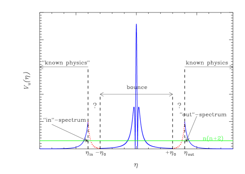
Figure 1: The shape of the potential in our bounce model. The usual assumption is that the potential starts as the full line growing curve in the region indicated “known physics”, then extends all the way to the corresponding full line decaying curve in the other known physics region with no special characteristics involved. In particular, the potential is thus assumed to have a global maximum somewhere in between, with perhaps a few irrelevant features on top of an otherwise regular curve. This means that once the mode has crossed such a potential, it will evolve through without noticeable change, except perhaps in its amplitude, but no dependence in the wavenumber can be introduced. By contrast, the actual potential we obtained in our model must follow first the same growing full curve, then drop as the dotted line in an essentially unknown way (hence the question mark), then connect to the actual bounce part. This is followed by another largely unknown piece connecting the really knwon physics. Clearly, the mode intersects this potential many times, and as the bounce transition itself changes the spectrum in a wavelength dependent way.

One way to perform a bounce, not necessarily taking into account the perhaps essential ingredients of the abovementionned scenarios, consists in using pure general relativity with a scalar field in a potential, provided the spatial sections are positively curved[2]. In this case, a comoving wavelength is just an eigenvalue of the Laplace operator on the 3-sphere, namely $k^{2}=n(n+2)$, with $n\in\mathbb{N}$ (in practice, given the current constraints on the curvature of space, the relevant modes are for $100\lesssim n\lesssim 10^{7}$) and the corresponding perturbation equation of motion can be cast in the form

$$u^{\prime\prime}+\left[n(n+2)-\frac{\theta^{\prime\prime}}{\theta}-3\mathcal{K}(1-c_{{}_{\rm S}}^{2})\right]u\equiv u^{\prime\prime}+\left[n(n+2)-V_{u}\left(\eta\right)\right]u=0\,,$$ (1)

thereby defining the potential $V_{u}(\eta)$ as a function of the conformal time $\eta$. The variable $u$ is related to the Bardeen gravitational potential $\Phi$ through

$$\Phi\equiv\frac{\kappa}{2}(\rho+p)^{1/2}u=\frac{\sqrt{3\kappa}}{2}\frac{{\mathcal{H}}}{a^{2}\theta}u,$$ (2)

where the conformal Hubble factor $\mathcal{H}$ is defined by the scale factor $a(\eta)$ through $\mathcal{H}\equiv a^{\prime}/a$ and the function $\theta$ is

$$\theta\equiv\frac{1}{a}\biggl{(}\frac{\rho}{\rho+p}\biggr{)}^{1/2}\biggl{(}1-\frac{3{\mathcal{K}}}{\kappa\rho a^{2}}\biggr{)}^{1/2}=\frac{1}{a}\biggl{(}\frac{3}{2\Gamma}\biggr{)}^{1/2}\,.$$ (3)

while

$$c_{{}_{\rm S}}^{2}\equiv\frac{p^{\prime}}{\rho^{\prime}}=-\frac{1}{3}\left(1+2\frac{\varphi^{\prime\prime}}{\mathcal{H}\varphi^{\prime}}\right).$$ (4)

stands for the “sound velocity”.

When the bounce is approximated by the Taylor expansion (see Ref. MPD for the specific form of the coefficients),

$$a(\eta)=a_{0}\biggl{[}1+\frac{1}{2}\biggl{(}\frac{\eta}{\eta_{0}}\biggr{)}^{2}+\delta\biggl{(}\frac{\eta}{\eta_{0}}\biggr{)}^{3}+\frac{5}{24}(1+\xi)\biggl{(}\frac{\eta}{\eta_{0}}\biggr{)}^{4}\biggr{]}\,,$$ (5)

the potential $V_{u}$ in Eq. (1) takes the shape indicated at the center of Fig. 1, whose essential properties are captured in the approximation $V_{u}(\eta)\simeq-C_{\Upsilon}\delta(\eta)$, with $C_{\Upsilon}\propto(\eta_{0}^{2}-1)^{-1/2}\ll 1$, the last inequality holding when the bounce is the shortest non NEC violating ($\eta_{0}$ close to unity). With such a $\delta$ potential, Eq. (1), which is formally equivalent to a “time”–independent Schrödinger equation, can be solved and give a transition matrix relating the dominant $D_{\pm}$ and subdominant $S_{\pm}$ modes of the contracting ($-$) and expanding ($+$) phases, namely

$$\begin{pmatrix}D_{+}\cr S_{+}\end{pmatrix}=\begin{pmatrix}T_{11}&T_{12}\cr T_{21}&T_{22}\end{pmatrix}\begin{pmatrix}D_{-}\cr S_{-}\end{pmatrix}\,,$$ (6)

and one finds[2] that the transfer matrix leading behaviour is

$$T-\mathbf{1}\propto-\frac{i}{\sqrt{\Upsilon n(n+2)}}\begin{pmatrix}1&1\cr-1&-1\end{pmatrix}$$ (7)

i.e. it contains a term proportional to the inverse of the wavenumber. Note also that since none of the matrix element vanishes, one expects the spectrum to exhibit specific properties that still need be investigated in details.

It should be noted, by way of conclusions, that the matrix of Eq. (7), obtained as a solution of a Schödinger-like equation, complies with the associated requirements of conservation of “probabilities” (namely that the reflection and transmission coefficients sum up to unity), unitarity of the $S-$matrix that can be built out of it and, in the symmetric $\delta=0$ case, of time-reversal invariance[3].

References

• [1] See M.Β Gasperini and G.Β Veneziano, Phys. Rep. 373, 1 (2003) and references therein.
• [2] J.Β Martin and P.Β Peter, Phys. Rev. D 68, 103517, (2003); Phys. Rev. Lett. 92, 061301 (2004) and references therein.
• [3] J.Β Martin and P.Β Peter, in preparation.