Abstract

We consider a generalisation of the DGP model, by adding a second brane with localised curvature, and allowing for a bulk cosmological constant and brane tensions. We study radion and graviton fluctuations in detail, enabling us to check for ghosts and tachyons. By tuning our parameters accordingly, we find bigravity models that are free from ghosts and tachyons. These models will lead to large distance modifications of gravity that could be observable in the near future.

1 Introduction

Where does the force of gravity come from? Anyone unfortunate enough to be near a strongly gravitating object, such as a black hole, would say “from the curvature of spacetime”. In a weaker gravitational field, we measure fluctuations about some background spacetime [1]. These fluctuations correspond to spin-2 particles called gravitons. Traditionally, we now say that “gravity comes from the exchange of massless gravitons”. We believe this because it reproduces Newton’s Law of gravitation, and that is well tested experimentally. But how well is Newton’s Law really tested? The truth is that our experimental knowledge of gravity only covers distances between $0.2$mm and $10^{26}$cm. The lower bound is as a result of Cavendish experiments, and the upper bound corresponds to 1% of the current Hubble length. In units of $\bar{h}=c=1$, this is equivalent to an energy scale

$$10^{-31}~{}\textrm{eV}<p<10^{-3}~{}\textrm{eV}$$ (1)

Perhaps, therefore, we should alter our previous statement. Gravity at the experimental scale (1) could be due to the exchange of massless and/or massive particles, so long as the masses are less than $10^{-31}~{}\textrm{eV}$. Indeed, massive gravitons appear automatically in some higher derivative gravity theories [2]. The simplest non-trivial scenario would contain a single massive graviton [1]. If we have a combination of gravitons of many different masses, we have multigravity [3, 4, 5, 6, 7, 8]. In this paper, we will encounter bigravity [9, 10]. This is the simplest example of multigravity, in which gravity is mediated by both a massless graviton and a single ultralight graviton.

Multigravity is clearly of interest from a purely theoretical point of view. However, it is also of interest to phenomenologists because it predicts new gravitational physics at very large distances. At distances beyond the Compton wavelength of the ultralight mode, the ultralight mode is turned off, and gravity is mediated by the massless mode alone. Large distance modifications of gravity have been in vogue recently, as they could offer an explanation to the current acceleration of the universe [11, 12, 13, 14, 15, 16].

Unfortunately, there are number of problems with many existing models of modified gravity. One very serious problem is the presence of ghosts (see, for example,  [3, 17, 18, 19, 20]). Although the “AdS brane” model in [9] is ghost-free, modifications of gravity are hidden behind the AdS horizon. The six dimensional model of Kogan et al [6] is also thought to be ghost-free, although this has not been confirmed as the model is too difficult to work with. The DGP model [21], meanwhile, is simple, ghost-free, and even predicts new infra-red physics, that could one day be observable. However, it is not a bigravity model; gravity is due to a resonance of continuum modes.

Let us describe the DGP model in more detail. It is given by the following action

$$S_{\textrm{DGP}}=M^{3}\int_{\textrm{bulk}}\sqrt{g}R(g)+m_{pl}^{2}\int_{\textrm{brane}}\sqrt{\gamma}R(\gamma)$$ (2)

In other words, we have a four-dimensional Minkowski brane embedded in a five-dimensional Minkowski bulk. The key ingredient is the brane localised curvature, $R(\gamma)$. This could be generated by quantum corrections, if matter were present on the brane. Localised curvature can also appear in string theory [22, 23]. In the DGP model, Newton’s Law is reproduced up to a distance $r=m_{pl}^{2}/2M^{3}$. Beyond this scale the behaviour of gravity is five-dimensional.

In this paper, we will consider a generalisation of the DGP model. We will add a second brane with localised curvature. We will also allow for a bulk cosmological constant, and for the branes to have tension. Since the extra dimension is finite, we will get a discrete graviton mass spectrum. Our aim is to ask the following question: is it possible to obtain an interesting modified theory of gravity without introducing ghosts and tachyons? The answer will be “yes”. For certain parameter regions, we will discover bigravity models that are tachyon and ghost-free, leading to potentially observable new physics in the infra-red. It is interesting to note that a single DGP-like brane in a compact extra dimension also has a discrete mass spectrum, but does not exhibit bigravity [24].

The rest of this paper will be organised as follows: in section 2, we will describe our set up in more detail, giving the bulk and boundary equations of motion. In section 3, we will derive solutions for the background spacetime. We will perturb about this background in section 4, arriving at the linearised equations of motion. In section 5 we will focus on the radion mode. This corresponds to fluctuations in the brane separation. We will calculate its effective action to quadratic order, in order to determine whether or not it is a ghost. For de Sitter branes we will find that the radion is tachyonic. In section 6, we will turn our attention to the gravitons. We will derive the mass spectrum, and show that we can have observable bigravity. We will also check for ghosts by calculating the graviton effective action. In section 7, we will play around with our parameters until we find a bigravity model that is ghost-free, and might one day lead to observable, new, infra-red physics. Section 8 will contain some final remarks. In particular, we will discuss some important issues, such as the famous van Dam-Veltman-Zakharov (vDVZ) discontinuity [25, 26], and the recently discovered strong coupling problems in massive gravity [27, 28]. Finally, the appendix contains a detailed calculation of the mass spectrum for AdS branes.

2 The Set Up

Consider two $3$-branes embedded in a five-dimensional bulk spacetime. For simplicity we assume that there is $\mathbb{Z}_{2}$ symmetry across each brane. This means that we can focus on the manifold, $\mathcal{M}$, which has one brane as its “left-hand” boundary, $\partial\mathcal{M}_{L}$, and the other brane as its “right-hand” boundary, $\partial\mathcal{M}_{R}$. The entire bulk is now given by two copies of $\mathcal{M}$.

Our set up is described by the following action

$$S=S_{\textrm{bulk}}+S_{\textrm{brane}},$$ (3)

where the contribution from the bulk is given by

$$S_{\textrm{bulk}}=2M^{3}\int_{\mathcal{M}}\sqrt{g}(R-2\Lambda)+\sum_{i=L,R}~{}4M^{3}\int_{\partial\mathcal{M}_{i}}\sqrt{g^{(i)}}K^{(i)}+2\int_{\mathcal{M}}L_{m}.$$ (4)

Here $M$ is the five-dimensional Planck mass, and $g_{ab}$ is the bulk metric with corresponding Ricci scalar, $R$. We have expilicitly included a bulk cosmological constant, $\Lambda$, which can be positive, negative or zero. Any additional contributions from matter in the bulk appear in $L_{m}$. For $i=L$, $R$, $g^{(i)}_{ab}$ is the induced metric on $\partial\mathcal{M}_{i}$, and $K^{(i)}_{ab}$ is the extrinsic curvature of $\partial\mathcal{M}_{i}$ in $\mathcal{M}$. Notice that $S_{\textrm{bulk}}$ contains an overall factor of two because of the $\mathbb{Z}_{2}$ symmetry.

The brane part of the action is given by

$$S_{\textrm{brane}}=\sum_{i=L,R}~{}\int_{\partial\mathcal{M}_{i}}\sqrt{g^{(i)}}\left(-\sigma_{i}+2M^{3}r_{i}\mathcal{R}^{(i)}\right)+\sum_{i=L,R}~{}\int_{\partial\mathcal{M}_{i}}\mathcal{L}_{m}^{(i)}$$ (5)

where for $i=L$, $R$, $\sigma_{i}$ is the tension of the brane at $\partial\mathcal{M}_{i}$. $\mathcal{L}_{m}^{(i)}$ gives the contribution from any additional matter on the brane. We have also allowed for some localised curvature by including the four-dimensional Ricci scalar, $\mathcal{R}^{(i)}$ on each brane. This is a DGP-like kinetic term [21], whose contribution is weighted by the distance $r_{i}$ in each case. At this stage we make no assumption about the magnitude, or even the sign of the $r_{i}$.

The bulk equations of motion are given by the Einstein equations

$$R_{ab}-\frac{1}{2}Rg_{ab}=-\Lambda g_{ab}+\frac{1}{2M^{3}}T_{ab}$$ (6)

where $T_{ab}$ is the energy momentum tensor for additional matter in the bulk. We also need to impose boundary conditions at the branes. For $i=L,~{}R$, these are given by the $\mathbb{Z}_{2}$ symmetric Israel equations [29] at $\partial\mathcal{M}_{i}$

$$K^{(i)}_{ab}=\frac{\sigma_{i}}{12M^{3}}g^{(i)}_{ab}-r_{i}\left[\mathcal{R}^{(i)}_{ab}-\frac{1}{6}\mathcal{R}^{(i)}g^{(i)}_{ab}\right]+\frac{1}{2M^{3}}\left[\mathcal{T}^{(i)}_{ab}-\frac{1}{3}\mathcal{T}^{(i)}g^{(i)}_{ab}\right]$$ (7)

Here $\mathcal{T}^{(i)}_{ab}$ corresponds to the energy momentum tensor for additional matter on $\partial\mathcal{M}_{i}$, and $\mathcal{T}^{(i)}$ is its trace.

3 Background solutions

In this section we will derive the metric, $\bar{g}_{ab}$, for the background spacetimes. These correspond to solutions of the equations of motion when no additional matter is present in the bulk, or on the branes. In other words

$$T_{ab}=\mathcal{T}^{(i)}_{ab}=0$$ (8)

Let us introduce coordinates $x^{a}=(x^{\mu},z)$, and assume that the brane at $\partial\mathcal{M}_{i}$ satisfies $z=z_{i}$, where $z_{L}=0$ and $z_{R}=l>0$. In order for us to trust our analysis, we need to assume that

$$M>\sqrt{\frac{|\Lambda|}{6}},~{}\frac{1}{l}$$ (9)

Now seek solutions of the form

$$ds^{2}=\bar{g}_{ab}dx^{a}dx^{b}=a^{2}(z)\tilde{g}_{\mu\nu}dx^{\mu}dx^{\nu}+dz^{2}.$$ (10)

where $\tilde{g}_{\mu\nu}$ describes a maximally symmetric four-dimensional spacetime, with Riemann tensor

$$\tilde{R}_{\mu\nu\alpha\beta}=\kappa\lambda^{2}\left(\tilde{g}_{\mu\alpha}\tilde{g}_{\nu\beta}-\tilde{g}_{\mu\beta}\tilde{g}_{\nu\alpha}\right).$$ (11)

where $\kappa=0,\pm 1$ for Minkowski, de Sitter and anti-de Sitter space respectively.

The Einstein equations in the bulk give the following differential equations for $a(z)$

$$\left(\frac{a^{\prime}}{a}\right)^{2}=\kappa\frac{\lambda^{2}}{a^{2}}-\frac{\Lambda}{6},\qquad\frac{a^{\prime\prime}}{a}=-\frac{\Lambda}{6}$$ (12)

By solving these, we find that for $-l\leq z\leq l$ [30, 31, 32]

$$a(z)=\begin{cases}\frac{\lambda}{k}\cos\left[\pm k(|z|-c)\right]&\Lambda=6k^{2},\quad\kappa=1~{}\textrm{only}\\ \lambda\left[c\pm\kappa|z|\right]&\Lambda=0,\quad\quad\kappa=0,~{}1\\ \frac{\lambda}{2k}\left[e^{\pm k(|z|-c)}-\kappa e^{\mp k(|z|-c)}\right]&\Lambda=-6k^{2},~{}\kappa=0,\pm 1,\end{cases}$$ (13)

where $c$ is an integration constant. We are free to define a length scale by setting $a(0)=1$. This fixes a relationship between $\lambda$ and $c$:

$$\lambda=\begin{cases}k/\cos(kc)&\Lambda=6k^{2},\quad\kappa=1~{}\textrm{only}\\ 1/c&\Lambda=0,\quad\quad\kappa=0,~{}1\\ 2k/\left[e^{\mp kc}-\kappa e^{\pm kc}\right]&\Lambda=-6k^{2},~{}\kappa=0,\pm 1,\end{cases}$$ (14)

For each of the solutions (13), the $\mathbb{Z}_{2}$ symmetry about $z=0$ is explicit, whereas the symmetry about $z=l$ can be seen when we identify $z$ with $z+2l$. When we have a negative bulk cosmological constant, these solutions correspond to those found in [33, 34, 35, 36].

The Israel equations on $\partial\mathcal{M}_{i}$ give us the following boundary conditions

$$\theta_{i}\frac{a^{\prime}(z_{i})}{a(z_{i})}=\frac{\sigma_{i}}{12M^{3}}-\kappa r_{i}\frac{\lambda^{2}}{a^{2}(z_{i})}$$ (15)

where $\theta_{L}=-1$ and $\theta_{R}=+1$. For the special case of $\Lambda=-6k^{2}$, $\kappa=0$, these equations give the usual Randall-Sundrum fine tuning of brane tensions [37]. Finally, we note that the cosmological constant on the brane at $\partial\mathcal{M}_{i}$ is given by

$$\Lambda_{i}=3\kappa\frac{\lambda^{2}}{a^{2}(z_{i})}.$$ (16)

and shall henceforth refer to the branes as flat, de Sitter or anti-de Sitter, when $\kappa=0,\pm 1$ respectively.

4 Metric Perturbations

We shall now consider perturbations about the background solutions (13) we have just derived. We will allow additional matter to be present on the branes, but not in the bulk. Let us define $g_{ab}=\bar{g}_{ab}+\delta g_{ab}$ to be the perturbed metric. We will work in Gaussian Normal coordinates so that

$$\delta g_{\mu z}=\delta g_{zz}=0.$$ (17)

Since we have no additional bulk matter, we can take the metric to be transverse-tracefree in the bulk. In other words, $\delta g_{\mu\nu}=\chi_{\mu\nu}$, where

$$\tilde{}\nabla_{\nu}\chi^{\nu}_{\mu}=\chi^{\mu}_{\mu}=0.$$ (18)

Here $\tilde{}\nabla$ is the covariant derivative with respect to the Minkowski, de Sitter or anti de Sitter metric $\tilde{g}_{\mu\nu}$. In this choice of gauge, the linearised bulk equations of motion are given by

$$\left[\frac{\tilde{}\nabla^{2}-4\kappa\lambda^{2}}{a^{2}}+\frac{\partial^{2}}{\partial z^{2}}+\frac{2\Lambda}{3}\right]\chi_{\mu\nu}=0.$$ (19)

where we have used equation (12).

Unfortunately, we can no longer assume that the branes are fixed at $z=z_{i}$. The presence of matter on the branes will cause them to bend [38]. In general, they will now be positioned at $z=z_{i}+f_{i}(x)$, for some function $f_{i}$ that depends only on the $x^{\mu}$. This makes it difficult to apply the Israel equations at the branes. To get round this we apply a gauge transformation that fixes $\partial\mathcal{M}_{L}$, and another that fixes $\partial\mathcal{M}_{R}$ [39], without spoiling the Gaussian Normal condition (17). This gives rise to two coordinate patches that are related by a gauge transformation in the region of overlap. We will call the patch that fixes $\partial\mathcal{M}_{L}$, the left-hand coordinate patch, and the one that fixes $\partial\mathcal{M}_{R}$, the right-hand patch.

To fix $\partial\mathcal{M}_{L}$, we make the following coordinate transformation

$$z\to z-f_{L}(x),\qquad x_{\mu}\to x_{\mu}+a^{2}(z)\partial_{\mu}f_{L}\int_{0}^{z}\frac{dy}{a^{2}(y)}$$ (20)

$\partial\mathcal{M}_{L}$ is now fixed at $z=0$, although $\partial\mathcal{M}_{R}$ is at $z=l+f_{R}-f_{L}$. The metric perturbation in this patch is given by

$$\delta g_{\mu\nu}=\chi^{(L)}_{\mu\nu}=\chi_{\mu\nu}-2a^{2}\tilde{}\nabla_{\mu}\tilde{}\nabla_{\nu}f_{L}\int_{0}^{z}\frac{dy}{a^{2}(y)}+2\frac{a^{\prime}}{a}f_{L}\bar{g}_{\mu\nu}$$ (21)

Similarly, to fix $\partial\mathcal{M}_{R}$, let

$$z\to z-f_{R}(x),\qquad x_{\mu}\to x_{\mu}+a^{2}(z)\partial_{\mu}f_{R}\int_{l}^{z}\frac{dy}{a^{2}(y)}$$ (22)

Now we have $\partial\mathcal{M}_{R}$ at $z=l$ but with $\partial\mathcal{M}_{L}$ at $z=f_{L}-f_{R}$. The metric perturbation is given by

$$\delta g_{\mu\nu}=\chi^{(R)}_{\mu\nu}=\chi_{\mu\nu}-2a^{2}\tilde{}\nabla_{\mu}\tilde{}\nabla_{\nu}f_{R}\int_{l}^{z}\frac{dy}{a^{2}(y)}+2\frac{a^{\prime}}{a}f_{R}\bar{g}_{\mu\nu}$$ (23)

We are now ready to use the Israel equations (7) to give linearised boundary conditions at each brane. At $\partial\mathcal{M}_{i}$, we have

$$\left[-\frac{\theta_{i}}{2}\frac{\partial}{\partial z}+\frac{\sigma_{i}}{12M^{3}}+\frac{r_{i}}{2a^{2}}\left(\tilde{}\nabla^{2}-4\kappa\lambda^{2}\right)\right]\chi_{\mu\nu}=-\left(\theta_{i}+2r_{i}\frac{a^{\prime}}{a}\right)\left[\tilde{}\nabla_{\mu}\tilde{}\nabla_{\nu}+\kappa\frac{\lambda^{2}}{a^{2}}\bar{g}_{\mu\nu}\right]f_{i}\\ -\frac{1}{2M^{3}}\left[\mathcal{T}^{(i)}_{\mu\nu}-\frac{1}{3}\mathcal{T}^{(i)}\bar{g}_{\mu\nu}\right]$$ (24)

where everything is evaluated at $z=z_{i}$. In deriving equation (24), we have made repeated use of equations (12) and (15).

Note that if we take the trace of equation (24), and use the fact that $\chi_{\mu\nu}$ is transverse-tracefree, we get

$$\left(\theta_{i}+2r_{i}\frac{a^{\prime}(z_{i})}{a(z_{i})}\right)\left[\frac{\tilde{}\nabla^{2}+4\kappa\lambda^{2}}{a^{2}}\right]f_{i}=\frac{\mathcal{T}^{(i)}}{6M^{3}}$$ (25)

This clearly shows that matter on the brane does indeed cause the brane to bend.

The general perturbation is made up of three parts: a radion, plane wave gravitons, and a particular solution that depends explicitly on the matter sources, $\mathcal{T}_{\mu\nu}^{(i)}$. The gravitons will be discussed in section 6. In the next section we will concentrate on the radion.

5 The Radion

5.1 Radion wavefunction

The radion mode, $\chi_{\mu\nu}^{\textrm{(rad)}}$, corresponds to fluctuations in the brane separation. It is in addition to the fluctuation caused explicitly by the matter on the brane, according to equation (25). The radion exists because equation (25) can have non-trivial solutions, $f_{i}$, even when $\mathcal{T}^{(i)}_{\mu\nu}=0$. Clearly then, the best way to see the radion is to consider a situation where we have no matter on the branes. Let us begin with a transverse-tracefree gauge in the bulk

$$\delta g_{\mu\nu}=\chi_{\mu\nu}^{\textrm{(rad)}}$$ (26)

with the branes positioned at $z=z_{i}+f_{i}(x)$. The fields, $f_{i}(x)$, are yet to be determined. $\chi_{\mu\nu}^{\textrm{(rad)}}$ satisfies equation (19), with the following boundary conditions at $\partial\mathcal{M}_{i}$

$$\left[-\frac{\theta_{i}}{2}\frac{\partial}{\partial z}+\frac{\sigma_{i}}{12M^{3}}+\frac{r_{i}}{2a^{2}}\left(\tilde{}\nabla^{2}-4\kappa\lambda^{2}\right)\right]\chi^{\textrm{(rad)}}_{\mu\nu}=-\left(\theta_{i}+2r_{i}\frac{a^{\prime}}{a}\right)\left[\tilde{}\nabla_{\mu}\tilde{}\nabla_{\nu}+\kappa\frac{\lambda^{2}}{a^{2}}\bar{g}_{\mu\nu}\right]f_{i}$$ (27)

where, again, everything is evaluated at $z=z_{i}$. Motivated by the tensor structure on the right-hand side of equation (24), we look for solutions to (19) of the form

$$\chi^{\textrm{(rad)}}_{\mu\nu}=\mu(z)\left(\tilde{}\nabla_{\mu}\tilde{}\nabla_{\nu}+\kappa\frac{\lambda^{2}}{a^{2}}\bar{g}_{\mu\nu}\right)\phi$$ (28)

where we have introduced a scalar field, $\phi(x)$, which we will call the radion field. Note that since $\chi^{\textrm{(rad)}}_{\mu\nu}$ is transverse-tracefree, we must have

$$\left[\tilde{}\nabla^{2}+4\kappa\lambda^{2}\right]\phi=0$$ (29)

This means that the radion field, $\phi$, has mass $m^{2}=-4\kappa\lambda^{2}$. When $\kappa=0$, the radion is massless, whereas for $\kappa=-1$, it is massive. For $\kappa=1$, the radion is tachyonic, signalling an instability for de Sitter branes [40].

Given the ansatz (28), we solve (19) to get an expression for $\mu(z)$.

$$\mu(z)=\begin{cases}\alpha+\beta z&\textrm{for $\Lambda=\kappa=0$}\\ aa^{\prime}\left[\alpha+\beta\int^{z}\frac{dy}{\left(aa^{\prime}\right)^{2}}\right]&\textrm{otherwise}\end{cases}$$ (30)

However, these expressions for $\mu(z)$ are too general. We find that $\chi_{\mu\nu}^{\textrm{(rad)}}$ contains terms which are pure gauge, and therefore unphysical. In fact, when $\Lambda=\kappa=0$, $\chi_{\mu\nu}^{\textrm{(rad)}}$ can be completely gauged away by the following coordinate tranformation

$$x^{\mu}\to x^{\mu}+(\alpha+\beta z)\partial_{\mu}\phi,\qquad z\to z-\beta\phi$$ (31)

When we apply the boundary conditions (24), we find that $f_{L}=f_{R}=0$. This means that there is no physical radion, and no matter-independant brane bending.

For every other case, the radion cannot be gauged away completely, so we are left with a physical radion mode. We can remove the term proportional to $\alpha$ in $\chi_{\mu\nu}^{\textrm{(rad)}}$ by taking

$$x^{\mu}\to x^{\mu}+\frac{1}{2}\alpha aa^{\prime}\partial_{\mu}\phi,\qquad z\to z+\frac{1}{2}\alpha\kappa\lambda^{2}\phi.$$ (32)

but we can do nothing about the other term. The physical radion perturbation is therefore given by equation (28) with

$$\mu(z)=aa^{\prime}\int^{z}\frac{dy}{\left(aa^{\prime}\right)^{2}}$$ (33)

Notice that we have set $\beta=1$ by absorbing it into the definition of $\phi$. Finally, the boundary conditions (27) give the $f_{i}$ in terms of $\phi(x)$. Making use of equations (12) and (15), we get

$$f_{i}(x)=\frac{1}{2}\left[\frac{1~{}}{v_{i}a(z_{i})a^{\prime}(z_{i})}-\kappa\lambda^{2}\int^{z_{i}}\frac{dy}{\left(aa^{\prime}\right)^{2}}\right]\phi(x)$$ (34)

where

$$v_{i}=1+2\theta_{i}r_{i}\frac{a^{\prime}(z_{i})}{a(z_{i})}$$ (35)

Note that equation (34) also imposes a relationship between $f_{L}(x)$ and $f_{R}(x)$.

5.2 Radion effective action

In braneworld theories that exhibit modification of gravity at large distances, we often find that the radion field is a ghost (see, for example, [17, 18]). We therefore need to check whether this is the case in any of our models. We do this by calculating the radion effective action to quadratic order, following [18] (see [41] for the supersymmetric case).

Let us work with the left-hand coordinate patch, which has the branes positioned at $z=0$ and $z=l+\delta l(x)$, where $\delta l=f_{R}-f_{L}$. The metric perturbation is given by

$$\delta g_{\mu\nu}=\chi_{\mu\nu}^{\textrm{(rad)}}-2a^{2}\tilde{}\nabla_{\mu}\tilde{}\nabla_{\nu}f_{L}\int_{0}^{z}\frac{dy}{a^{2}(y)}+2\frac{a^{\prime}}{a}f_{L}\bar{g}_{\mu\nu},\qquad\delta g_{\mu z}=\delta g_{zz}=0$$ (36)

In order to integrate out the extra dimension, it is convenient to have both branes fixed. We can do this with the following coordinate transformation

$$z\to z-B(z)\delta l,\qquad x_{\mu}\to x_{\mu}+a^{2}(z)\partial_{\mu}(\delta l)\int^{z}_{0}\frac{B(y)}{a^{2}(y)}dy$$ (37)

where $B(z)$ is some differentiable function for $0\leq z\leq l$, satisfying $B(0)=0$ and $B(l)=1$. While this transformation ensures that $\delta g_{\mu z}$ is still zero, the price we pay for fixed branes is that we now have non-vanishing $\delta g_{zz}$. More precisely,

$$\delta g_{\mu\nu}=h_{\mu\nu}=\chi_{\mu\nu}^{\textrm{(rad)}}+2\frac{a^{\prime}}{a}\left[f_{L}+\delta lB(z)\right]\bar{g}_{\mu\nu}-2a^{2}\tilde{}\nabla_{\mu}\tilde{}\nabla_{\nu}f_{L}\int_{0}^{z}\frac{dy}{a^{2}(y)}$$

$$\qquad\qquad\qquad\qquad\qquad\qquad-2a^{2}\tilde{}\nabla_{\mu}\nabla_{\nu}(\delta l)\int_{0}^{z}\frac{B(y)}{a^{2}(y)}dy$$ (38)

$$\delta g_{zz}=h_{zz}=2\delta lB^{\prime}(z)$$ (39)

To quadratic order, the effective action is given by

$$S_{\textrm{eff}}=-M^{3}\int_{0}^{l}dz\int d^{4}x\sqrt{\bar{g}}~{}h^{ab}\delta E_{ab}-\sum_{i=L,R}M^{3}\int_{z=z_{i}}d^{4}x\sqrt{\bar{g}}~{}h^{\mu\nu}\delta\Theta^{(i)}_{\mu\nu}$$ (40)

where $\delta E_{ab}$ and $\delta\Theta^{(i)}_{\mu\nu}$ are the expansions, to linear order, of the bulk and boundary equations of motion respectively.

$$E_{ab} = R_{ab}-\frac{1}{2}Rg_{ab}+\Lambda g_{ab}$$ (41)

$$\Theta^{(i)}_{\mu\nu} = K^{(i)}_{\mu\nu}-K^{(i)}g^{(i)}_{\mu\nu}+\frac{\sigma_{i}}{4M^{3}}g^{(i)}_{\mu\nu}+r_{i}\left[\mathcal{R}^{(i)}_{\mu\nu}-\frac{1}{2}\mathcal{R}^{(i)}g^{(i)}_{\mu\nu}\right]$$ (42)

We find that $\delta E_{\mu\nu}$ and $\delta\Theta^{(i)}_{\mu\nu}$ are identically zero [18]. After integrating out a total derivative in $z$, we arrive at the following effective action for the radion

$$S_{\textrm{eff}}=-3M^{3}\left[\Delta\left(\frac{1}{v_{i}a(z_{i})a^{\prime}(z_{i})}\right)-\kappa\lambda^{2}\int_{0}^{l}\frac{dy}{\left(aa^{\prime}\right)^{2}}\right]\int d^{4}x\sqrt{\tilde{g}}~{}\phi\left(\tilde{}\nabla^{2}+4\kappa\lambda^{2}\right)\phi$$ (43)

where $\Delta Q_{i}=Q_{R}-Q_{L}$.

5.3 “No ghost” bounds

The radion field, $\phi$, becomes a ghost when the coefficient of its kinetic term becomes negative. This would indicate a sickness in our theory. We therefore require that

$$\Delta\left(\frac{1}{v_{i}a(z_{i})a^{\prime}(z_{i})}\right)-\kappa\lambda^{2}\int_{0}^{l}\frac{dy}{\left(aa^{\prime}\right)^{2}}\leqslant 0$$ (44)

We shall not consider what this means for de Sitter branes, because the radion is tachyonic, even if it is not a ghost. However, for flat and anti-de Sitter branes it is worth considering this condition in more detail.

When $\Lambda=\kappa=0$, there is no radion, and therefore nothing to worry about. When $\Lambda=-6k^{2}$, $\kappa=0$, we have $a(z)=e^{-k|z|}$, and the condition (44) demands that

$$\frac{1}{1-2kr_{R}}\geqslant\frac{e^{-2kl}}{1+2kr_{L}}$$ (45)

Now consider anti-de Sitter branes with $\Lambda=-6k^{2}$, $\kappa=-1$. Given that the warp factor $a(z)=\frac{\lambda}{k}\cosh\left[k\left(|z|-c\right)\right]$, we can show that the condition (44) requires that

$$\frac{\frac{\sinh(2kc)}{1+2kr_{R}\tanh[k(l-c)]}+\frac{\sinh[2k(l-c)]}{1+2kr_{L}\tanh(kc)}-\sinh(2kl)}{\sinh[2k(l-c)]\sinh(2kc)}\leqslant 0$$ (46)

Here we will mainly be interested in the “symmetric” case ($c=l/2$), so that (46) simplifies to

$$\frac{1}{1+2kr_{R}\tanh(kl/2)}+\frac{1}{1+2kr_{L}\tanh(kl/2)}\leqslant 2\cosh(kl)$$ (47)

To sum up, we have shown that we can avoid ghost-like radions by placing certain bounds on the parameters in our model. While this is of no real use for tachyonic de Sitter branes, it will be important when considering flat and anti-de Sitter branes.

6 Gravitons

In this section we will consider graviton perturbations in detail. We will ask two important questions: (i) when does the graviton become a ghost, and (ii) do we have a bigravity model? As with the radion, we can derive “no ghost” bounds for the graviton by calculating the effective action. To establish whether or not we have bigravity, we need to find the graviton mass spectrum. For bigravity, we expect to see a massless mode and an ultralight mode [3, 4, 5, 9, 6, 7, 8, 10, 14]. This will lead to modifications of gravity at large distances. However, it is important to note that this modified behaviour may never be observable. For example, for AdS branes there is a danger that the Compton wavelength of the ultralight graviton is larger than the horizon size [9]. Once we have established the existance of an ultralight graviton, we will check that it could one day lead to interesting observations.

6.1 Graviton mass spectrum

Consider the metric perturbation decomposed into plane waves

$$\delta g_{\mu\nu}(x,z)=\sum_{m}\chi_{\mu\nu}^{(m)}(x)u_{m}(z)$$ (48)

where

$$\left(\tilde{}\nabla^{2}-2\kappa\lambda^{2}\right)\chi_{\mu\nu}^{(m)}=m^{2}\chi_{\mu\nu}^{(m)}.$$ (49)

From a four-dimensional perspective, $\chi_{\mu\nu}^{(m)}$ corresponds to a transverse-tracefree, spin 2 particle of mass, $m$ [42, 43, 44, 45, 46, 47, 48, 49, 50, 51].

We now insert (48) into the equations of motion (19) and (24). Since we are interested in plane waves, and the radion has already been accounted for, we set $f_{i}=\mathcal{T}^{(i)}_{\mu\nu}=0$. The equations of motion become

$$\left(\frac{m^{2}-2\kappa\lambda^{2}}{a^{2}}+\frac{\partial^{2}}{\partial z^{2}}+\frac{2\Lambda}{3}\right)u_{m}(z)=0,$$ (50)

in the bulk, with boundary conditions

$$\left[-\frac{\theta_{i}}{2}\frac{\partial}{\partial z}+\frac{\sigma_{i}}{12M^{3}}+\frac{r_{i}}{2a^{2}}\left(m^{2}-2\kappa\lambda^{2}\right)\right]u_{m}(z)=0$$ (51)

at $z=z_{i}$. Different eigenstates are orthogonal, so that for $m\neq n$,

$$\int_{-l}^{l}dz~{}\frac{1}{a^{2}(z)}\left[1+2r_{L}\delta(z)+2r_{R}\delta(z-l)\right]u_{m}(z)u_{n}(z)=0$$ (52)

We can always find a zero mode that satisfies the boundary conditions

$$u_{0}(z)=A_{0}a^{2}(z)$$ (53)

where $A_{0}$ is some normalisation constant. We shall now look for massive modes for the flat and anti-de Sitter branes of primary interest, taking each case in turn.

6.1.1 $\Lambda=\kappa=0$

Since $a(z)\equiv 1$, the bulk equation (50) is particularly simple. In addition to the zero mode (53), we find a number of massive modes

$$u_{m}(z)=A_{m}\cos(m|z|)+B_{m}\sin(m|z|)$$ (54)

for some constants $A_{m}$, $B_{m}$, that are yet to be determined. The boundary conditions require that

$$r_{L}mA_{m}+B_{m}=0$$ (55)

$$\left[r_{R}m\cos(ml)+\sin(ml)\right]A_{m}+\left[r_{R}m\sin(ml)-\cos(ml)\right]B_{m}=0$$ (56)

Note that we have used the fact that $\sigma_{i}=0$. If we want a non-trivial solution for $A_{m}$ and $B_{m}$, we are only allowed quantised values of $m$, satisfying

$$\left(m^{2}r_{L}r_{R}-1\right)\sin(ml)=m\left(r_{L}+r_{R}\right)\cos(ml).$$ (57)

The main KK tower will therefore be made up of states with $m_{\textrm{heavy}}\gtrsim 1/l$. Are there any ultralight states? To answer this, consider (57) when $m\ll 1/l$. We find a mode with mass

$$m_{\textrm{light}}\approx\sqrt{\frac{6\left(l+r_{L}+r_{R}\right)}{l^{3}+3l^{2}(r_{L}+r_{R})+6lr_{L}r_{R}}}$$ (58)

This is indeed much smaller than $1/l$, if we choose $x=r_{L}/l$ and $y=r_{R}/l$ so that

$$\epsilon^{2}=\frac{\left(1+x+y\right)}{1+3(x+y)+6xy}$$ (59)

where $|\epsilon|\ll 1$.

6.1.2 $\Lambda=-6k^{2}$; $\kappa=0$

We now consider the Randall-Sundrum I model with brane-localised curvature terms. This time we have $a(z)=e^{-k|z|}$. By solving the bulk equation (50), we again find a number of massive modes [52, 32]

$$u_{m}(z)=A_{m}J_{2}(me^{k|z|}/k)+B_{m}Y_{2}(me^{k|z|}/k)$$ (60)

where $J_{n}$ and $Y_{n}$ are Bessel’s functions of integer order $n$. The boundary conditions (51) imply

$$A_{m}\left[-\theta_{i}J_{1}(me^{kz_{i}}/k)+mr_{i}e^{kz_{i}}J_{2}(me^{kz_{i}}/k)\right]\\ +B_{m}\left[-\theta_{i}Y_{1}(me^{kz_{i}}/k)+mr_{i}e^{kz_{i}}Y_{2}(me^{kz_{i}}/k)\right]=0$$ (61)

On this occasion we have used the fact $-k\theta_{i}=\sigma_{i}/12M^{3}$. Equation (61) is of course two equations, one for $i=L$ and one for $i=R$. For these to have non-trivial solutions for $A_{m}$ and $B_{m}$, we again find that $m$ is quantised accordingly

$$\left[J_{1}(m/k)+mr_{L}J_{2}(m/k)\right]\left[-Y_{1}(me^{kl}/k)+mr_{R}e^{kl}Y_{2}(me^{kl}/k)\right]\\ =\left[Y_{1}(m/k)+mr_{L}Y_{2}(m/k)\right]\left[-J_{1}(me^{kl}/k)+mr_{R}e^{kl}J_{2}(me^{kl}/k)\right]$$ (62)

We now focus on the case when the brane separation is large, $l\gtrsim 1/k$. In this instance, the main KK tower is made up of states with mass $m_{\textrm{heavy}}\gtrsim ke^{-kl}$ [52, 32, 53]. Is there an ultralight state? Consider (62) when $m\ll ke^{-kl}$, and use the fact that

$$J_{1}(t) =\frac{t}{2}-\frac{t^{3}}{16}+\mathcal{O}\left(t^{5}\right) Y_{1}(t) =-\frac{2}{\pi t}+\frac{t}{\pi}\ln\left(\frac{t}{2}\right)+\mathcal{O}\left(t\right)$$ (63)

$$J_{2}(t) =\frac{t^{2}}{8}+\mathcal{O}\left(t^{4}\right) Y_{2}(t) =-\frac{4}{\pi t^{2}}-\frac{1}{\pi}\mathcal{O}\left(t^{2}\ln(t)\right)$$ (64)

for $|t|\ll 1$. To leading order, we find a mode with mass

$$m_{\textrm{light}}\approx 2ke^{-kl}\sqrt{\frac{\left(kr_{L}+\frac{1}{2}\right)e^{2kl}+kr_{R}-\frac{1}{2}}{\left(kr_{L}+\frac{1}{2}\right)\left(kr_{R}+\frac{1}{2}\right)e^{2kl}-k(l+r_{L}+r_{R})-\left(kr_{L}-\frac{1}{2}\right)\left(kr_{R}-\frac{1}{2}\right)e^{-2kl}}}$$ (65)

This is much smaller than $ke^{-kl}$, as long as we choose $x=kr_{L}$ and $y=kr_{R}$, so that

$$\epsilon^{2}=\frac{\left(x+\frac{1}{2}\right)e^{2kl}+y-\frac{1}{2}}{\left(x+\frac{1}{2}\right)\left(y+\frac{1}{2}\right)e^{2kl}-(kl+x+y)-\left(x-\frac{1}{2}\right)\left(y-\frac{1}{2}\right)e^{-2kl}}$$ (66)

where $|\epsilon|\ll 1$.

Now consider the opposite regime, when the brane separation is small, $l\ll 1/k$. The mass spectrum is well approximated by the expressions given in section 6.1.1, when $\Lambda=\kappa=0$: the heavy modes have mass $m_{\textrm{heavy}}\gtrsim 1/l$, and the mass of the light mode is given by (58). Note that (65) reduces to (58) in this limit, and is therefore valid for all values of $l$.

6.1.3 $\Lambda=-6k^{2}$; $\kappa=-1$

Finally, we consider AdS branes with brane-localised curvature. We shall focus on the “symmetric” case, where $a(z)=\frac{\lambda}{k}\cosh\left[k\left(|z|-\frac{l}{2}\right)\right]$ and $\lambda=k/\cosh\left[kl/2\right]$. A detailed analysis can be found in appendix A. There we see that the eigenstates, $u_{m}(z)$, are given in terms of hypergeometric functions (see equation (94)). Again, the boundary conditions impose a quantisation condition on $m$ (see equation (101)).

When the branes are far apart ($l\gtrsim 1/k$), the situation is very similar to the case when $r_{i}=0$ [9]. We have bigravity, but the Compton wavelength of the ultralight graviton is larger than the size of the AdS horizon. Large distance modifications of gravity will therefore never be observable.

Now consider the opposite regime, when the branes are very close together ($l\ll 1/k$). Again, the expressions given in section 6.1.1 give a good estimate for the mass spectrum. The horizon size on either brane is given by $1/\lambda\approx 1/k$. Large distance modifications of gravity could therefore be observable, as long as,

$$\frac{1}{l}\gg m_{\textrm{light}}>k$$ (67)

6.2 Graviton effective action

Now that we know the graviton mass spectrum, we are ready to calculate the corresponding effective action to check for ghosts. Since we have assumed that $f_{i}=0$, we can immediately insert the metric (48) into equation (40). Making use of the orthogonality condition (52), we find that the effective action, to quadratic order, is given by

$$S_{\textrm{eff}}=\sum_{m}C_{m}\int d^{4}x\sqrt{\tilde{g}}~{}\chi^{(m)\mu\nu}\left(\tilde{\nabla}^{2}-2\kappa\lambda^{2}-m^{2}\right)\chi^{(m)}_{\mu\nu}$$ (68)

where

$$C_{m}=\frac{M^{3}}{2}\int_{0}^{l}dz~{}\left[\frac{u_{m}(z)}{a(z)}\right]^{2}\left[1+r_{L}\delta(z)+r_{R}\delta(z-l)\right]$$ (69)

As an aside, we will also examine the coupling of each mode to matter on the branes. To do this, we allow for $\mathcal{T}^{(i)}_{\mu\nu}\neq 0$, giving additional terms

$$S_{\textrm{matter}}=\sum_{i=L,R}\sum_{m}\int d^{4}x\sqrt{\tilde{g}}~{}\frac{u_{m}(z_{i})}{2}\chi^{(m)\mu\nu}\mathcal{T}_{\mu\nu}^{(i)}$$ (70)

If we define the canonically normalised fields as

$$\widehat{\chi}^{(m)}_{\mu\nu}=\sqrt{C_{m}}\chi^{(m)}_{\mu\nu}$$ (71)

we see that the mode of mass, $m$ has the following coupling to matter on $\partial\mathcal{M}_{i}$,

$$g^{(i)}_{m}=\frac{u_{m}(z_{i})}{2\sqrt{C_{m}}}.$$ (72)

We can relate these couplings to the four-dimensional Planck mass, $M_{i}$ on $\partial\mathcal{M}_{i}$. At the intermediate energy scale, $m_{\textrm{heavy}}\gg p\gg m_{\textrm{light}}$, gravity is due to both the massless and ultralight mode. We deduce that,

$$\frac{1}{M_{i}^{2}}=2\left[g^{(i)}_{0}\right]^{2}+2\left[g^{(i)}_{\textrm{light}}\right]^{2}$$ (73)

6.3 “No ghost” bounds

We can now ask whether or not we have any ghost-like gravitons. If we assume that $\chi^{(m)}_{\mu\nu}$ is real, it is clear that this mode is not a ghost, provided

$$C_{m}\geqslant 0$$ (74)

Since we are not too concerned about the ultra-violet behaviour of this theory, we only need to impose this condition on the massless and ultralight modes. For the massless mode (53), this is equivalent to

$$\int_{0}^{l}a^{2}(z)~{}dz+\sum_{i=L,R}r_{i}a^{2}(z_{i})\geqslant 0$$ (75)

For each case of interest, this gives

$$l+r_{L}+r_{R}\geqslant 0 \textrm{for}~{}\Lambda=\kappa=0$$ (76)

$$\left(kr_{L}+\frac{1}{2}\right)e^{2kl}+kr_{R}-\frac{1}{2}\geqslant 0 \textrm{for}~{}\Lambda=-6k^{2},~{}\kappa=0$$ (77)

$$k\left(r_{L}+r_{R}\right)+\tanh\left(\frac{kl}{2}\right)+\frac{kl}{2}\textrm{sech}^{2}\left(\frac{kl}{2}\right)\geqslant 0$$ for “symmetric” AdS branes (78)

In addition we also require that $C_{\textrm{light}}\geqslant 0$. However, it will not be necessary to evaluate this explicitly in all cases, as most bigravity models will be ruled out by the radion bounds (44) and the massless mode condition (75).

7 Analysis

The aim of this paper is to find a braneworld bigravity theory that is free of ghosts and tachyons. We saw in section 5 that tachyons appear on de Sitter branes in the form of the radion field, so we ruled these models out. Other types of brane have not been ruled out, and we showed in section 6.1 how one can choose parameters so that we get a model of bigravity. In this section we will check whether or not these choices are compatible with the “no ghost” bounds of sections 5.3 and 6.3. We will also keep in mind the validity bound (9), and the hope that bigravity will lead to modifications of gravity that will one day be observable.

7.1 $\Lambda=\kappa=0$

Let us begin with the case $\Lambda=\kappa=0$. For bigravity, we need equation (59) to hold for $|\epsilon|\ll 1$ (recall that $x=r_{L}/l$ and $y=r_{R}/l$). We have no radion to worry about, although we do need to be careful with the gravitons. The massless graviton is not a ghost, as long as

$$1+x+y\geqslant 0$$ (79)

Now consider the plot of $x=r_{L}/l$ against $y=r_{R}/l$ shown in figure 1.

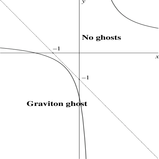
Figure 1: Analysis for $\Lambda=\kappa=0$.

The solid black line corresponds to a line of constant $|\epsilon|\ll 1$. As $x\to\infty$, $y\to 1/6\epsilon^{2}$, and vice-versa. The dotted line corresponds to $1+x+y=0$, and represents the boundary between the massless graviton being well behaved, and the appearance of a ghost. Since the solid line never crosses the dotted line, it is clear that we need $x,~{}y\geqslant 1/6\epsilon^{2}$. In other words, we need $r_{i}\gg l$.

We are now ready to check the behaviour of the ultralight mode. For simplicity, let $r_{L}=r_{R}=r\gg l$, so that

$$m_{\textrm{light}}\approx\sqrt{\frac{2~{}}{lr}}$$ (80)

If we use this along with equations (54) and (55), we find that

$$C_{\textrm{light}}\approx A_{m}^{2}M^{3}r\geqslant 0$$ (81)

The ultralight mode is not ghost, so we conclude that we have indeed found a bigravity model that is ghost-free. At intermediate energy scales, note that the Planck mass on either brane is given by

$$M_{i}^{2}=m^{2}_{pl}\approx M^{3}r$$ (82)

as we might have expected.

7.2 $\Lambda=-6k^{2};~{}l\ll 1/k;~{}\kappa=0,-1$

We now turn our attention to the case where $\Lambda=-6k^{2},~{}\kappa=0,-1$, with $l\ll 1/k$. In this limit, the mass spectrum is the same as for $\Lambda=\kappa=0$, and the graviton bounds (77) and (78), are reduced to (79). The analysis will therefore be very similar to what we have just done for $\Lambda=\kappa=0$, as we would expect by continuity. There are, however, a couple of other things to consider now. We have a radion to worry about (see equations (45) and (47)), and for $\kappa=-1$, we need to ensure that any infra-red modifications of gravity will not be hidden behind the AdS horizon.

For simplicity, let us again assume that $r_{L}=r_{R}=r\gg l$. In both cases we find that there is an upper bound on the value of $r$

$$r<\begin{cases}1/2k&\textrm{for $\kappa=0$}\\ 2/k^{2}l&\textrm{for $\kappa=-1$}\end{cases}$$ (83)

For $\kappa=0$, this is due to the radion becoming a ghost [53]. For $\kappa=-1$, however, the radion is not a problem, and the bound is due to the condition, $m_{\textrm{light}}>k$. This ensures that long distance modifiactions of gravity may one day be observable.

The upper bounds on $r$ are not too troublesome, as long as we take $k$ to be very small.

7.3 $\Lambda=-6k^{2};~{}l\gtrsim 1/k;~{}\kappa=0$

Finally, we consider the (DGP) extension of the RS model, with the branes far apart. For bigravity, we need equation (66) to hold for $|\epsilon|\ll 1$ (recall that now we have $x=kr_{L}$ and $y=kr_{R}$). From equations (45) and (77) we have the following bounds

$$\frac{-1~{}}{y-\frac{1}{2}}\geqslant\frac{e^{-2kl}}{x+\frac{1}{2}}$$ to avoid a radion ghost (84)

$$x+\frac{1}{2}+\left(y-\frac{1}{2}\right)e^{-2kl}\geqslant 0$$ to avoid a (massless) graviton ghost (85)

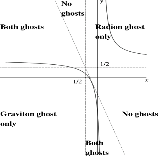
Figure 2: Analysis for $\Lambda=-6k^{2}$,  $\kappa=0$,  $l\gtrsim 1/k$.

Now consider the plot of $x=kr_{L}$ against $y=kr_{R}$ shown in figure 2. Again, the solid black line corresponds to a line of constant $|\epsilon|\ll 1$. The asymptotic behaviour is

$$y\to\frac{1+\coth(2kl)}{2\epsilon^{2}} ~{}\textrm{as}~{}x\to\infty$$

$$x\to\frac{\textrm{cosech}(2kl)}{2\epsilon^{2}} ~{}\textrm{as}~{}y\to\infty$$

The dotted lines correspond to boundaries, across which the “ghost-like” status of the theory changes. The diagonal line is given by $x+\frac{1}{2}+\left(y-\frac{1}{2}\right)e^{-2kl}=0$, whereas the horizontal and vertical lines are given by $y=1/2$ and $x=-1/2$ respectively. It is easy to check that the solid line never enters any of the “no ghost” regions indicated. This means that for this model to exhibit bigravity, either the radion, the graviton, or both, will become a ghost. The model is therefore rejected.

8 Conclusions

In this paper we have studied a class of braneworld models, with localised curvature on the branes. Some of these models give rise to bigravity, leading to large distance modifications of gravity for a four-dimensional observer. After checking for ghosts and tachyons, we rejected most, but not all of the models we had considered.

One of these well behaved models consists of a flat bulk ($\Lambda=0$) sandwiched in between two flat branes ($\kappa=0$) of zero tension. The branes are close together, and the curvature terms on the brane are large and positive ($r_{i}\gg l$). The mass spectrum is precisely that of bigravity. We have a massless graviton, an ultralight graviton, and a tower of heavy KK modes. The model is completely free of ghosts and tachyons.

To add some substance, let us put some numbers in. If we take $l\sim 10^{3}~{}(\textrm{eV})^{-1}$, and $r_{i}\sim 10^{59}~{}(\textrm{eV})^{-1}$, we find that

$$m_{\textrm{light}}\sim 10^{-31}~{}\textrm{eV},\qquad m_{\textrm{heavy}}\gtrsim 10^{-3}~{}\textrm{eV}.$$ (86)

These masses lie outside of the range for which gravity is well tested (1), so we have no contradiction with experiment. Since the four-dimensional Planck mass, $m_{pl}\sim 10^{18}~{}\textrm{GeV}$, we conclude from equation (82) that $M\sim 10^{-2}-10^{-1}~{}\textrm{eV}$. While the fundamental Planck scale is very low, it does not violate the validity bound (9), and exceeds the scale probed by Cavendish experiments ($10^{-3}~{}\textrm{eV}$). In principle there are cosmological and astrophysical bounds that one should consider, such as the effect on star cooling due to graviton emmision into the bulk. This will be left for future research.

Note that $m_{\textrm{light}}\sim 10^{-31}~{}\textrm{eV}$ is just about heavy enough for us to expect interesting observations today. This could be important in trying to explain cosmic acceleration. If we wanted to reduce this mass even further, we would have to increase $r$. Even a small increase would push the Planck mass below the Cavendish scale. Curiously, we seem to be in just the right place to start seeing interesting new physics, either in the infra-red, or the ultra-violet.

We can go beyond this model by switching on a small AdS curvature in the bulk, and still get ghost-free bigravity. Although a tachyon appears for de Sitter branes, this is not the case for flat and anti-de Sitter branes. When the bulk AdS length is of the same order as the brane separation, we find that ghost-free bigravity becomes impossible.

By checking for ghosts and tachyons in our models, we have carried out the first important tests of viability. However, we should be aware that there are other possible problems. As with all models of massive gravity, we should be concerned with the famous vDVZ discontinuity [25, 26]. Our linearised equations of motion (24) suggest that this may well be an issue. This is especially true for the case $\Lambda=\kappa=0$, as there is no “brane-bending” effect that could cancel off any unwanted degrees of freedom (see, for example,  [54, 55]). Even our AdS brane model will suffer this problem. This is a surprise, as it is often said that there is no vDVZ discontinuity in AdS space [56, 57]. However, this result relies on the graviton mass going to zero faster than the inverse horizon size. In order to ensure that we had observable bigravity, we demanded the opposite of this.

Crucially, there may be a way around this problem. Vainshtein et al [58, 59], have argued that the perturbative expansion in Newton’s constant in [25, 26], is inconsistent, as the graviton mass goes to zero. Specifically, the standard linearised analysis near a heavy source is only valid at distances

$$r\geqslant\left(\frac{r_{M}}{m^{4}}\right)^{\frac{1}{5}}$$ (87)

where $r_{M}$ is the Schwarzschild radius of the source, and $m$ is the graviton mass. To see if a mass discontinuity really is present, we need to calculate the Schwarzschild solution on a brane, and compare it to the standard four-dimensional massless result. This is a highly non-trivial exercise that is beyond the scope of this paper.

For Pauli-Fierz theory [1], the breakdown of the linearised analysis has been linked to strong coupling phenomena at the following scale [27]

$$E_{\textrm{strong}}\sim\left(\frac{l_{pl}}{m^{4}}\right)^{-\frac{1}{5}}$$ (88)

where $l_{pl}$ is the Planck length. Large terms in the full propagator tend to signal this problem. Unfortunately, we might expect our theory to suffer the same fate. We can see this by looking at $h_{zz}$ in a fixed wall gauge (see equation (39)). By the mean value theorem, there exists $z_{0}\in[0,l]$ such that $B^{\prime}(z_{0})=1/l$. For small $l$, it is clear that $h_{zz}$ can be very large.

A similar strong coupling scale also exists in the DGP model [60, 61]. However, it has recently been argued that this scale could be unphysical, and is just a result of the naive perturbative expansion [62]. Clearly, both the mass discontiniuty and strong coupling problems are highly contentious issues at the moment. For this reason we have focused on the possible existence of ghosts in our models. There is no contention there: ghosts are undesirable, but can be avoided.

There is still much to do. It would be very interesting to study the phenomenology of these models in more detail, particularly in the context of cosmic acceleration. Coincidentally, we have been forced to choose a brane separation $l\sim 10^{3}~{}(\textrm{eV})^{-1}$, which agrees with the brane separation chosen in [63]. In [63], the mass spectrum is motivated by a discretized Randall-Sundrum model, with $l$ chosen so that there is a small effective cosmological constant. Would the presence of an ultralight mode in the spectrum affect these results? We would probably expect the answer to be “no”, because the dominant contribution to the vacuum energy would still come from the heavier modes. Nevertheless, it is worthy of further investigation.

Our models could certainly be generalised in a number of ways. We could consider more branes, abandon $\mathbb{Z}_{2}$ symmetry, or even introduce higher derivative terms in the bulk and on the brane. Branes embedded in solutions to Gauss-Bonnet gravity have been the subject of much research recently (see, for example [64, 65]), motivated by the link to string theory. Indeed, it would also be nice if our models, or at least some generalisation, could be derived from a more fundamental theory [22, 23]. However, the high degree of fine tuning could prove an obstacle in this respect.

Let us end by summarising our main result: we have discovered braneworld models that exhibit bigravity, without introducing ghosts. Recall that bigravity naturally gives rise to new gravitational physics in the infra-red. The new physics occurs when the massive graviton “switches off”, at distances beyond its Compton wavelength. Our models are an improvement on the ghost-free model given in [9], because they lead to potentially observable modifications of gravity. In [9], all modifications are hidden behind the AdS horizon.

Acknowledgements

I would like to thank John March-Russell, Valery Rubakov, Graham Ross, Syksy Räsänen, and Ben Gripaios for helpful dicussions. In particular, I would like to thank John and Graham for proof reading this article. Thanks must also go to Ben, Ro, Ash and Perks for being a constant source of inspiration, Leppos and Beyoncé. And to Bruno Cheyrou for being the new Zidane. AP was funded by PPARC.

Appendix A Mass spectrum for AdS branes

For “symmetric” AdS branes, we have

$$a(z)=\frac{\lambda}{k}\cosh\left[k\left(|z|-\frac{l}{2}\right)\right],\qquad\lambda=k/\cosh\left[kl/2\right]$$ (89)

We want to find the massive eigenstates, $u_{m}(z)$, that satisfy equation (50).

$$\left[\left(\frac{m^{2}+2\lambda^{2}}{a^{2}}\right)+\frac{\partial^{2}}{\partial z^{2}}-4k^{2}\right]u_{m}(z)=0$$ (90)

Let $u_{m}(z)=v_{m}(y)/a^{2}(z)$, where $y=\tanh^{2}\left(k\left(|z|-\frac{l}{2}\right)\right)$. We find that $v_{m}$ satisfies the following hypergeometric equation

$$y(1-y)v_{m}^{\prime\prime}(y)+\frac{1}{2}(1-7y)v_{m}^{\prime}(y)+\frac{m^{2}-4\lambda^{2}}{4\lambda^{2}}v_{m}(y)=0$$ (91)

The solution is given in terms of hypergeometric functions [9]

$$v_{m}(y)=A_{m}F\left(a_{m},b_{m},\frac{1}{2};y\right)+B_{m}\sqrt{y}F\left(a_{m}+\frac{1}{2},b_{m}+\frac{1}{2},\frac{3}{2};y\right)$$ (92)

where $A_{m}$, $B_{m}$ are arbitrary constants and

$$a_{m}=\frac{5}{2}+\sqrt{\frac{9}{4}+\frac{m^{2}}{\lambda^{2}}},\qquad b_{m}=\frac{5}{2}-\sqrt{\frac{9}{4}+\frac{m^{2}}{\lambda^{2}}}$$ (93)

The eigenstates are therefore given by

$$u_{m}(z)=\textrm{sech}^{2}\left[k\left(|z|-\frac{l}{2}\right)\right]\left\{A_{m}F\left(a_{m},b_{m},\frac{1}{2};\tanh^{2}\left[k\left(|z|-\frac{l}{2}\right)\right]\right)\right.\\ \left.+B_{m}\tanh\left[k\left(|z|-\frac{l}{2}\right)\right]F\left(a_{m}+\frac{1}{2},b_{m}+\frac{1}{2},\frac{3}{2};\tanh^{2}\left[k\left(|z|-\frac{l}{2}\right)\right]\right)\right\}$$ (94)

where we have absorbed some constants into $A_{m}$ and $B_{m}$. After some tedious algebra, we see that the boundary conditions (51) give the following

$$A_{m}\alpha_{m}+B_{m}\beta_{m} = 0$$ (95)

$$A_{m}\tilde{}\alpha_{m}+B_{m}\tilde{\beta}_{m} = 0$$ (96)

where

$$\alpha_{m} = 4kta_{m}b_{m}\left(t^{2}-1\right)F\left(a_{m}+1,b_{m}+1,\frac{3}{2};t^{2}\right)$$ (97)

$$\qquad+\left(4kt+\bar{r}m^{2}\right)F\left(a_{m},b_{m},\frac{1}{2};t^{2}\right)$$

$$\beta_{m} = \left(\frac{\Delta r}{2}\right)m^{2}tF\left(a_{m}+\frac{1}{2},b_{m}+\frac{1}{2},\frac{3}{2};t^{2}\right)$$ (98)

$$\tilde{}\alpha_{m} = \left(\frac{\Delta r}{2}\right)m^{2}F\left(a_{m},b_{m},\frac{1}{2};t^{2}\right)$$ (99)

$$\tilde{\beta}_{m} = \frac{4}{3}kt^{2}\left(t^{2}-1\right)\left(a_{m}+\frac{1}{2}\right)\left(b_{m}+\frac{1}{2}\right)F\left(a_{m}+\frac{3}{2},b_{m}+\frac{3}{2},\frac{5}{2};t^{2}\right)$$ (100)

$$\qquad+\left(k\left(5t^{2}-1\right)+\bar{r}m^{2}t\right)F\left(a_{m}+\frac{1}{2},b_{m}+\frac{1}{2},\frac{3}{2};t^{2}\right)$$

Here $t=\tanh\left(kl/2\right)$ and $\bar{r}=(r_{L}+r_{R})/2$. By demanding that there exists a non-trivial solution for $A_{m}$ and $B_{m}$, we find a quantisation condition for $m$

$$\alpha_{m}\tilde{\beta}_{m}=\tilde{}\alpha_{m}\beta_{m}$$ (101)

References

- [1] M. Fierz and W. Pauli, “On relativistic wave equations for particles of arbitrary spin in an electromagnetic field,” Proc. Roy. Soc. Lond. A173 (1939) 211–232.
- [2] A. Hindawi, B. A. Ovrut, and D. Waldram, “Consistent Spin-Two Coupling and Quadratic Gravitation,” Phys. Rev. D53 (1996) 5583–5596, hep-th/9509142.
- [3] I. I. Kogan, S. Mouslopoulos, A. Papazoglou, G. G. Ross, and J. Santiago, “A three three-brane universe: New phenomenology for the new millennium?,” Nucl. Phys. B584 (2000) 313–328, hep-ph/9912552.
- [4] I. I. Kogan and G. G. Ross, “Brane universe and multigravity: Modification of gravity at large and small distances,” Phys. Lett. B485 (2000) 255–262, hep-th/0003074.
- [5] I. I. Kogan, S. Mouslopoulos, A. Papazoglou, and G. G. Ross, “Multi-brane worlds and modification of gravity at large scales,” Nucl. Phys. B595 (2001) 225–249, hep-th/0006030.
- [6] I. I. Kogan, S. Mouslopoulos, A. Papazoglou, and G. G. Ross, “Multigravity in six dimensions: Generating bounces with flat positive tension branes,” Phys. Rev. D64 (2001) 124014, hep-th/0107086.
- [7] I. I. Kogan, “Multi(scale)gravity: A telescope for the micro-world,” astro-ph/0108220.
- [8] A. Papazoglou, “Brane-world multigravity,” hep-ph/0112159.
- [9] I. I. Kogan, S. Mouslopoulos, and A. Papazoglou, “A new bigravity model with exclusively positive branes,” Phys. Lett. B501 (2001) 140–149, hep-th/0011141.
- [10] T. Damour and I. I. Kogan, “Effective lagrangians and universality classes of nonlinear bigravity,” Phys. Rev. D66 (2002) 104024, hep-th/0206042.
- [11] Supernova Cosmology Project Collaboration, S. Perlmutter et. al., “Measurements of Omega and Lambda from 42 High-Redshift Supernovae,” Astrophys. J. 517 (1999) 565–586, astro-ph/9812133.
- [12] Supernova Search Team Collaboration, A. G. Riess et. al., “Observational Evidence from Supernovae for an Accelerating Universe and a Cosmological Constant,” Astron. J. 116 (1998) 1009–1038, astro-ph/9805201.
- [13] C. Deffayet, “Cosmology on a brane in Minkowski bulk,” Phys. Lett. B502 (2001) 199–208, hep-th/0010186.
- [14] T. Damour, I. I. Kogan, and A. Papazoglou, “Non-linear bigravity and cosmic acceleration,” Phys. Rev. D66 (2002) 104025, hep-th/0206044.
- [15] A. Lue, R. Scoccimarro, and G. Starkman, “Differentiating between Modified Gravity and Dark Energy,” astro-ph/0307034.
- [16] A. Lue, R. Scoccimarro, and G. D. Starkman, “Probing Newton’s constant on vast scales: DGP gravity, cosmic acceleration and large scale structure,” astro-ph/0401515.
- [17] R. Gregory, V. A. Rubakov, and S. M. Sibiryakov, “Opening up extra dimensions at ultra-large scales,” Phys. Rev. Lett. 84 (2000) 5928–5931, hep-th/0002072.
- [18] L. Pilo, R. Rattazzi, and A. Zaffaroni, “The fate of the radion in models with metastable graviton,” JHEP 07 (2000) 056, hep-th/0004028.
- [19] S. L. Dubovsky and V. A. Rubakov, “Brane-induced gravity in more than one extra dimensions: Violation of equivalence principle and ghost,” Phys. Rev. D67 (2003) 104014, hep-th/0212222.
- [20] S. L. Dubovsky and M. V. Libanov, “On brane-induced gravity in warped backgrounds,” hep-th/0309131.
- [21] G. R. Dvali, G. Gabadadze, and M. Porrati, “4D gravity on a brane in 5D Minkowski space,” Phys. Lett. B485 (2000) 208–214, hep-th/0005016.
- [22] S. Corley, D. A. Lowe, and S. Ramgoolam, “Einstein-Hilbert action on the brane for the bulk graviton,” JHEP 07 (2001) 030, hep-th/0106067.
- [23] I. Antoniadis, R. Minasian, and P. Vanhove, “Non-compact Calabi-Yau manifolds and localized gravity,” Nucl. Phys. B648 (2003) 69–93, hep-th/0209030.
- [24] G. R. Dvali, G. Gabadadze, M. Kolanovic, and F. Nitti, “The power of brane-induced gravity,” Phys. Rev. D64 (2001) 084004, hep-ph/0102216.
- [25] H. van Dam and M. J. G. Veltman, “Massive and massless Yang-Mills and gravitational fields,” Nucl. Phys. B22 (1970) 397–411.
- [26] V. I. Zakharov JETP Lett. 12 (1970) 312.
- [27] N. Arkani-Hamed, H. Georgi, and M. D. Schwartz, “Effective field theory for massive gravitons and gravity in theory space,” Ann. Phys. 305 (2003) 96–118, hep-th/0210184.
- [28] M. D. Schwartz, “Constructing gravitational dimensions,” Phys. Rev. D68 (2003) 024029, hep-th/0303114.
- [29] W. Israel, “Singular hypersurfaces and thin shells in general relativity,” Nuovo Cim. B44S10 (1966) 1.
- [30] R. Gregory and A. Padilla, “Nested braneworlds and strong brane gravity,” Phys. Rev. D65 (2002) 084013, hep-th/0104262.
- [31] R. Gregory and A. Padilla, “Braneworld instantons,” Class. Quant. Grav. 19 (2002) 279–302, hep-th/0107108.
- [32] A. Padilla, “Braneworld cosmology and holography,” hep-th/0210217.
- [33] N. Kaloper, “Bent domain walls as braneworlds,” Phys. Rev. D60 (1999) 123506, hep-th/9905210.
- [34] H. B. Kim and H. D. Kim, “Inflation and gauge hierarchy in Randall-Sundrum compactification,” Phys. Rev. D61 (2000) 064003, hep-th/9909053.
- [35] T. Nihei, “Inflation in the five-dimensional universe with an orbifold extra dimension,” Phys. Lett. B465 (1999) 81–85, hep-ph/9905487.
- [36] A. Karch and L. Randall, “Locally localized gravity,” JHEP 05 (2001) 008, hep-th/0011156.
- [37] L. Randall and R. Sundrum, “A large mass hierarchy from a small extra dimension,” Phys. Rev. Lett. 83 (1999) 3370–3373, hep-ph/9905221.
- [38] J. Garriga and T. Tanaka, “Gravity in the brane-world,” Phys. Rev. Lett. 84 (2000) 2778–2781, hep-th/9911055.
- [39] C. Charmousis, R. Gregory, and V. A. Rubakov, “Wave function of the radion in a brane world,” Phys. Rev. D62 (2000) 067505, hep-th/9912160.
- [40] Z. Chacko and P. J. Fox, “Wave function of the radion in the dS and AdS brane worlds,” Phys. Rev. D64 (2001) 024015, hep-th/0102023.
- [41] J. Bagger and M. Redi, “Radion effective theory in the detuned Randall-Sundrum model,” hep-th/0312220.
- [42] G. W. Gibbons and M. J. Perry, “Quantizing gravitational instantons,” Nucl. Phys. B146 (1978) 90.
- [43] B. Allen and T. Jacobson, “Vector two point functions in maximally symmetric spaces,” Commun. Math. Phys. 103 (1986) 669.
- [44] B. Allen and M. Turyn, “An evaluation of the graviton propagator in de Sitter space,” Nucl. Phys. B292 (1987) 813.
- [45] M. Turyn, “Curvature fluctuations in maximally symmetric spaces,” Phys. Rev. D39 (1989) 2951.
- [46] M. Turyn, “The graviton propagator in maximally symmetric spaces,” J. Math. Phys. 31 (1990) 669.
- [47] B. Allen, “The graviton propagator in de Sitter space,” Phys. Rev. D34 (1986) 3670.
- [48] A. Chodos and E. Myers, “Gravitational contribution to the Casimir energy in Kaluza- Klein theories,” Ann. Phys. 156 (1984) 412.
- [49] A. Higuchi and S. S. Kouris, “The covariant graviton propagator in de Sitter spacetime,” Class. Quant. Grav. 18 (2001) 4317–4328, gr-qc/0107036.
- [50] E. D’Hoker, D. Z. Freedman, S. D. Mathur, A. Matusis, and L. Rastelli, “Graviton and gauge boson propagators in AdS(d+1),” Nucl. Phys. B562 (1999) 330–352, hep-th/9902042.
- [51] A. Naqvi, “Propagators for massive symmetric tensor and p-forms in AdS(d+1),” JHEP 12 (1999) 025, hep-th/9911182.
- [52] L. Randall and R. Sundrum, “An alternative to compactification,” Phys. Rev. Lett. 83 (1999) 4690–4693, hep-th/9906064.
- [53] H. Davoudiasl, J. L. Hewett, and T. G. Rizzo, “Brane localized curvature for warped gravitons,” JHEP 08 (2003) 034, hep-ph/0305086.
- [54] S. B. Giddings, E. Katz, and L. Randall, “Linearized gravity in brane backgrounds,” JHEP 03 (2000) 023, hep-th/0002091.
- [55] C. Csaki, J. Erlich, and T. J. Hollowood, “Graviton propagators, brane bending and bending of light in theories with quasi-localized gravity,” Phys. Lett. B481 (2000) 107–113, hep-th/0003020.
- [56] I. I. Kogan, S. Mouslopoulos, and A. Papazoglou, “The m 0 limit for massive graviton in dS(4) and AdS(4): How to circumvent the van Dam-Veltman-Zakharov discontinuity,” Phys. Lett. B503 (2001) 173–180, hep-th/0011138.
- [57] M. Porrati, “No van Dam-Veltman-Zakharov discontinuity in AdS space,” Phys. Lett. B498 (2001) 92–96, hep-th/0011152.
- [58] A. I. Vainshtein, “To the problem of nonvanishing gravitation mass,” Phys. Lett. B39 (1972) 393–394.
- [59] C. Deffayet, G. R. Dvali, G. Gabadadze, and A. I. Vainshtein, “Nonperturbative continuity in graviton mass versus perturbative discontinuity,” Phys. Rev. D65 (2002) 044026, hep-th/0106001.
- [60] M. A. Luty, M. Porrati, and R. Rattazzi, “Strong interactions and stability in the DGP model,” JHEP 09 (2003) 029, hep-th/0303116.
- [61] V. A. Rubakov, “Strong coupling in brane-induced gravity in five dimensions,” hep-th/0303125.
- [62] G. Dvali, “Infrared modification of gravity,” hep-th/0402130.
- [63] G. Cognola, E. Elizalde, S. Nojiri, S. D. Odintsov, and S. Zerbini, “Multi-graviton theory from a discretized RS brane-world and the induced cosmological constant,” hep-th/0312269.
- [64] S. C. Davis, “Generalised Israel junction conditions for a Gauss-Bonnet brane world,” Phys. Rev. D67 (2003) 024030, hep-th/0208205.
- [65] J. P. Gregory and A. Padilla, “Braneworld holography in Gauss-Bonnet gravity,” Class. Quant. Grav. 20 (2003) 4221–4238, hep-th/0304250.