Cosmology from Rolling Massive Scalar Field on the
anti-D3 Brane of de Sitter Vacua

Abstract

We investigate a string-inspired scenario associated with a rolling massive scalar field on D-branes and discuss its cosmological implications. In particular, we discuss cosmological evolution of the massive scalar field on the ant-D3 brane of KKLT vacua. Unlike the case of tachyon field, because of the warp factor of the anti-D3 brane, it is possible to obtain the required level of the amplitude of density perturbations. We study the spectra of scalar and tensor perturbations generated during the rolling scalar inflation and show that our scenario satisfies the observational constraint coming from the Cosmic Microwave Background anisotropies and other observational data. We also implement the negative cosmological constant arising from the stabilization of the modulus fields in the KKLT vacua and find that this leads to a successful reheating in which the energy density of the scalar field effectively scales as a pressureless dust. The present dark energy can be also explained in our scenario provided that the potential energy of the massive rolling scalar does not exactly cancel with the amplitude of the negative cosmological constant at the potential minimum.

I Introduction

Cosmological inflation has become an integral part of the standard model of the universe review . Apart from being capable of removing the shortcomings of the standard big-bang cosmology, this paradigm has gained a good amount of support from the accumulated observational data. The recent measurement of the Wilkinson Microwave Anisotropy Probe (WMAP) WMAP1 ; WMAP2 in the Cosmic Microwave Background (CMB) made it clear that (i) the current state of the universe is very close to a critical density and that (ii) primordial density perturbations that seeded large-scale structure in the universe are nearly scale-invariant and Gaussian, which are consistent with the inflationary paradigm.

Inflation is often implemented with a single or multiple scalar-field models LR . In most of these models, at least one of the scalar fields undergoes a slow-roll period allowing an accelerated expansion of the universe. It then enters the regime of quasi-periodic oscillations, quickly oscillates and decays into particles leading to reheating. The late time acceleration of universe is supported by observations of high redshift supernovae and indirectly, by observations of the cosmic microwave background and galaxy clustering. The cosmic acceleration can be sourced by an exotic form of matter (dark energy) with a large negative pressure phiindustry . Therefore, the standard model in order to comply with the logical consistency and observation, should be sandwiched between inflation at early epoch and quintessence at late times. It is natural to ask whether one can construct a natural cosmological model using scalar fields to join the two ends without disturbing the thermal history of the universe. Attempts have been made to unify both these concepts using models with a single scalar field unifiedmodels .

Inspite of all the attractive features of cosmological inflation, its mechanism of realization still remains ad hoc. As inflation operates around the Planck’s scale, the needle of hope points towards the string theory. It is, therefore, not surprising that M/String theory inspired models are under active consideration in cosmology at present. It was recently been suggested that a rolling tachyon condensate, in a class of string theories, might have interesting cosmological consequences. Using the boundary conformal field theory (BCFT) technique, Sen s1 has shown that the decay of D-branes produces a pressure-less gas with a finite energy density that resembles a classical dust. He also shown that the same results can be extracted from the tachyon DBI effective action as1 . Rolling tachyon matter associated with unstable D-branes has an interesting equation of state $w$ which smoothly interpolates between $-1$ and 0. As the tachyon field rolls down the hill, the universe undergoes an accelerated expansion and at a particular epoch, the scale factor passes through the point of inflection marking the end of inflation. At late times the energy density of tachyon matter scales as $a^{-3}$, where $a$ is a scale factor. The tachyonic matter was, therefore, thought to provide an explanation for inflation at the early epochs and could contribute to some new form of cosmological dark matter at late times tachyonindustry . Unfortunately, the effective potentials for rolling tachyon do not contain free parameters that could be tuned to make the roll sufficiently slow to obtain enough inflation and required level of density perturbations KL . The situation could be remedied by invoking the large number of D-branes separated by distance much larger than $l_{s}$ (string scale). However, the number of branes turns out to be typically of the order of $10^{10}$. This scenario also faces difficulties associated with reheating and the formation of acoustics/kinks Frolov .

In this paper we consider a DBI type effective field theory of rolling massive scalar boson on the D-brane or anti-D brane obtained from string theory. We then consider this effective action for the massive excitation of the anti-D3 brane of the KKLT vacua, and study the cosmological evolution of the scalar rolling from some initial value. The warp factor, $\beta$, of the anti-D3 brane provides us an interesting possibility to resolve the problem of the large amplitude of density perturbations. We also take into account the contribution of the negative cosmological constant arising from the stabilization of the modulus fields in the KKLT vacua KKLT . This is important to avoid that the energy density of the rolling massive scalar over dominates the universe after inflation. The present critical density can be explained by considering both the minimum potential of the rolling scalar and the negative cosmological constant. We also evaluate the inflationary observables such as the spectral index of scalar perturbations and the tensor-to-scalar ratio, and examine the validity of this scenario by using a complication of latest observational data.

II Scalar rolling

Sen has discussed in s2 a general iterative procedure for constructing, in string field theory, a one parameter time-dependent solution describing the rolling of a tachyon away from its maximum. In the Wick rotated theory, the solution to order $\Lambda^{2}$ is

$$|\Psi\rangle = \Lambda|\phi_{0}\rangle-\Lambda^{2}\frac{b_{0}}{L_{0}}|\phi_{0}*\phi_{0}\rangle+{\cal O}(\Lambda^{3})\,,$$ (1)

where $L_{0}$ and $b_{0}$ are the zero mode of the world-sheet energy-momentum tensor and the ghost field $b$, respectively. The higher order terms involve on-shell scattering amplitude of external states $|\phi_{0}\rangle$. This state is related to the zero momentum tachyon vertex operator $V_{T}(0)$,i.e.,

$$|\phi_{0}\rangle=\cos(\omega X(0))V_{T}(0)c_{1}|0\rangle\,,$$ (2)

where $c_{1}$ is the first mode of the ghost field $c$, the world-sheet field $X$ is the Wick rotation of the space-time time coordinate $X^{0}$, and $\omega$, at leading order, is the mass of the tachyon field. At higher order, $\omega$ is a function of the parameter $\Lambda$ s2 . One can obtain a time-dependent solution after an inverse Wick rotation $x=-ix^{0}$ on the final result.

As has been discussed in s2 , one can make use of the above method to generate a one parameter time-dependent solution describing the oscillation of a positive mass² scalar field about the minimum of its potential. In this case there is no need for Wick rotation. For a scalar field $\phi$ of mass $m$, $|\phi_{0}\rangle$ is given by

$$|\phi_{0}\rangle = \cos(\omega X^{0}(0))V_{\phi}(0)c_{1}|0\rangle\,,$$ (3)

where again $V_{\phi}$ is the zero momentum vertex operator of the scalar field. At leading order, $\omega=m$ and at higher order it is a function of the parameter $\Lambda$.

One can also find the BCFT associated with the above massive scalar rolling solution. Since the final solution in string field theory (1) is obtained by iterating the initial solution (3), one may expect that this corresponds to a BCFT that is obtained by perturbing the original BCFT by the boundary term

$$\hat{\lambda}\int dt\cos(\omega X^{0}(t))V_{\phi}(t)\,,$$ (4)

where $\hat{\lambda}=\Lambda+{\cal O}(\Lambda^{2})$ and $t$ is a parameter labeling the boundary of the world-sheet. At the leading order, $\omega=m$ and at higher order it is a function of $\Lambda$. In this case also the higher-order terms are related to on-shell scattering amplitude of the above vertex operator s2 . The solution obtained in this way describes a one parameter family of BCFT, each member of which is related to the boundary conformal field theory describing the original D-brane system by a nearly marginal deformation. Time evolution of the sources of massless closed string fields can be extracted from the boundary state jp ; mbg ; sen2 . Unfortunately, the perturbed BCFT is not solvable, and hence we cannot explicitly compute the boundary state associated with this BCFT s2 .

In the present paper, however, we are interested in an effective action that might produce the above one parameter solution in field theory. Since the above solution has one parameter, the effective action should have only first derivative of the scalar field comment . Moreover, we expect that the effective action should have non-abelian $U(N)$ gauge symmetry when the original D-brane system involves $N$ coincident D-branes witten , or non-commutative $U(1)$ gauge symmetry when the original D-brane system carries background B-flux nsw .

Recently one of the present authors mrg1 discussed an effective action that includes a first derivative of the scalar fields which have the following vertex operators

$$V_{\phi} = \zeta_{i}\partial^{n}X^{i}e^{ik\cdot X}\,.$$ (5)

In above relation, the index $i$ runs over the transverse directions of the D_p-brane, i.e., $i=p+1,\cdots,25$, $\zeta_{i}$ represent the polarization of the scalar state, and $k^{a}$ with $a=0,1,\cdots,p$ is the momentum of the scalar state along the D_p-brane. Mass of the above vertex operator is $m^{2}=(n-1)/{\alpha^{\prime}}$ where $n$ is an integer number and $\sqrt{\alpha^{\prime}}$ is the string length scale. Hence, for $n\geq 2$ this vertex represents a massive scalar state. The disk level four-point amplitude of the above scalar has been evaluated in Ref. mrg1 . Then an expansion for the amplitude has been found that its leading order terms correspond to an action with a non-abelian gauge symmetry. Reducing the non-abelian symmetry to the abelian one in which we are interested, the leading couplings are consistent with the following Born-Infeld type action mrg1 :

$$S = -\int d^{p+1}xV(\phi)$$

$$\times\sqrt{-\det(\eta_{ab}+2\pi\alpha^{\prime}F_{ab}+\partial_{a}\phi^{i}\partial_{b}\phi_{i})}\,,$$

where $F_{ab}$ and $\phi^{i}$ are the gauge field strength and the scalar fields, respectively. The massive scalar potential is

$$V(\phi) = T_{p}\left(1+\frac{1}{2}m^{2}\phi^{i}\phi_{i}+\frac{1}{8}m^{4}(\phi^{i}\phi_{i})^{2}+\cdots\right)$$ (7)

$$= T_{p}e^{\frac{1}{2}m^{2}\phi^{i}\phi_{i}}\,,$$

where $T_{p}$ is the D$p$-brane tension. In the second line above we have speculated a closed form for the expansion.

The massless closed string fields can be added into the above effective action by the general grounds of covariance, T-duality, and by the fact that the world-sheet is disk, that is

$$S = -\int d^{p+1}xV(\phi)e^{-\Phi}$$

$$\times\sqrt{-\det(g_{ab}+B_{ab}+2\pi\alpha^{\prime}F_{ab}+\partial_{a}\phi^{i}\partial_{b}\phi_{i})},$$

where $\Phi$, $g_{ab}$ and $B_{ab}$ are the dilaton, metric and the anti-symmetric two tensor fields, respectively.

One may use the world-sheet conformal field theory technique mrgrm to evaluate the S-matrix element of two massive scalar states (5) and one massless closed string vertex operators to confirm the closed string couplings in the above action. The scalar fields are not massless so, unlike the massless case, the expansion of the amplitude will not be a low-energy expansion. In order to find an appropriate expansion for the S-matrix element, one may firstly evaluate the amplitude in the presence of the background B-flux mrg2 . The amplitude has then massless pole and infinite tower of massive poles. Using the fact that the effective field theory in this case is a non-commutative field theory, and that the non-commutative massive field theory has graviton-gauge field coupling as well as the scalar-scalar-gauge field coupling, then, one finds that the expansion of the amplitude should be around the massless pole. After finding the expansion, one may set the background B-flux to zero. The leading non-zero term of the expansion should then be consistent with the coupling of the scalar-scalar-massless closed string field extracted from the above action.

The construction of the massive effective action from S-matrix element can easily be carried out in the superstring theory. One needs only consider the analog of the massive vertex operators (5) in the superstring theory. It is argued in mrg1 that the action (II) is consistent with the leading order terms of the S-matrix element of four massive vertex operators in the superstring theory. The index $i$ in this case takes the values $i=p+1,\cdots,9$, and $m^{2}=(n-1)/(2\alpha^{\prime})$ with $n\geq 1$ for BPS D-branes in which we are interested. On the general grounds, one expects that the closed string fields $\Phi$, $B_{ab}$ and $g_{ab}$ have the coupling consistent with the action (II). In the superstring, there is also the RR massless closed string fields. One may study the S-matrix element of two massive scalar and one RR vertex operators to find the coupling of RR to the scalar fields. However, we are not interested in these couplings here.

In the present paper, we are interested in the cosmological evolution of the massive scalar rolling of BPS-D3-brane of type IIB string theory. In principle one can study this evolution in string field theory or in the BCFT as we already mentioned above. However, no analytical solution can be obtained in string field theory, and BCFT is not solvable in this case s2 . Hence we stick to the effective action (II) and find the cosmological evolution in this field theory.

In order to study the cosmological evolution of the D$3$-brane or anti-D$3$ brane, one has to assume that the extra six dimensions of type IIB string theory are frozen in a compact manifold such that evolution of the massive scalar field on the brane does not decompactify the internal manifold . Recently a construction of this compactification was reported by the authors in Ref. KKLT (KKLT). In the next section we review this construction.

III Review of KKLT vacua

The low energy effective action of string/M-theory in four dimension is described by $N=1$ supergravity,

$$S = \int d^{4}x\,\sqrt{-g}\biggl{[}\frac{M_{p}^{2}}{2}R+g^{\mu\nu}K_{a\bar{b}}\partial_{\mu}\varphi^{a}\partial_{\nu}\bar{\varphi}^{b}$$ (9)

$$-e^{K/M_{p}^{2}}\left(K^{a\bar{b}}D_{a}WD_{\bar{b}}\bar{W}-\frac{3}{M_{p}^{2}}|W|^{2}\right)$$

$$+\cdots\biggr{]},$$

where $a,b$ run over all complex moduli fields. In the above equation, the holomorphic function $W(\varphi^{a})$ is the superpotential, $K(\varphi^{a},\bar{\varphi}^{b})$ is the Kahler potential, $K_{a\bar{b}}=\partial^{2}K/\partial\varphi^{a}\partial\bar{\varphi}^{b}$ is the Kahler metric, and $D_{a}W$ is the Kahler derivative,

$$D_{a}W = \frac{\partial W}{\partial\varphi^{a}}+\frac{W}{M_{p}^{2}}\frac{\partial K}{\partial\varphi^{a}}\,.$$ (10)

The supersymmetry will be unbroken only for the vacua in which $D_{a}W=0$ for all $a$; the effective cosmological constant is thus non-positive. Some preferable choices of the Kahler potential $K$, and superpotential $W$ will be selected at the level of the fundamental string/M-theory. We set $M_{p}^{2}=1$ in the rest of this section.

Using the flux compactification of Type IIB string theory pm ; sg , the authors in Ref. sg used the following tree level functions for $K$ and $W$:

$$K = -3\ln[-i(\rho-\bar{\rho})]-\ln[-i(\tau-\bar{\tau})]$$ (11)

$$-\ln[-i\int_{M}\Omega\wedge\bar{\Omega}]\,,$$

$$W = \int_{M}G_{3}\wedge\Omega\,,$$ (12)

where $\Omega$ is the holomorphic three-form on the Calabi-Yau space and $G_{3}=F_{3}-\tau H_{3}$ where $F_{3}$ and $H_{3}$ are the R-R flux and the NS-NS flux, respectively, on the 3-cycles of the internal Calabi-Yau manifold, $\rho$ the volume modulus which includes the volume of Calabi-Yau space and an axion field coming from the R-R 4-form, $C_{(4)}$, and $\tau=C_{(0)}+ie^{-\Phi}$ is axion-dilaton modulus. Since $W$ is not a function of $\rho$,one has $K^{\rho\bar{\rho}}D_{\rho}WD_{\bar{\rho}}\bar{W}=3|W|^{2}$, which reduces the supergravity potential to

$${\cal V} = e^{K}\left(K^{i\bar{j}}D_{i}WD_{\bar{j}}\bar{W}\right)\,,$$ (13)

where $i,j$ run over all moduli fields except $\rho$.

It is argued in sg that the condition $D_{i}W=0$ fixes all complex moduli except $\rho$. This gives zero effective cosmological constant. On the other hand, the supersymmetric vacua that satisfies $D_{\rho}W=0$ gives $W=0$, whereas, non-supersymmetric vacua yield $W=W_{0}\neq 0$.

The flux $F_{3}$ and $H_{3}$ are also the sources for a warp factor pm ; sg . Therefore, models with flux are generically warped compactifications,

$$ds^{2}_{10} = e^{2A(y)}g_{\mu\nu}(x)dx^{\mu}dx^{\nu}$$ (14)

$$+e^{-2A(y)}\tilde{g}_{mn}(y)dy^{m}dy^{n}\,,$$

where the warp factor, $e^{A}$, can be computed in the regions closed to a conifold singularity of the Calabi-Yau manifold sg . The result for the warp factor is exponentially suppressed at the throat’s tip, depending on the fluxes as:

$$e^{A_{\rm min}}\sim\exp\left[-\frac{2\pi N}{3g_{s}M}\right]\,,$$ (15)

where $g_{s}$ is the string coupling constant, and integers $M$, $N$ are the R-R and NS-NS three-form flux, respectively. While the warp factor is of order one at generic points in the $y$-space, its minimum value can be extremely small given a suitable choice of fluxes.

In order to fix $\rho$ as well, KKLT KKLT added a non-perturbative correction ew to the superpotential, that is

$$K=K_{0}-3\ln[-i(\rho-\bar{\rho})]\,,$$ (16)

$$W=W_{0}+Ae^{ia\rho}\,,$$ (17)

where $A$ and $a$ are two constants. In this equation $W_{0}=\int G_{3}\wedge\Omega$ and $K_{0}=-\ln[-i(\tau-\bar{\tau})]-\ln[-i\int\Omega\wedge\bar{\Omega}]$ are evaluated at the above fixed moduli. Now the conditions $D_{i}W=0$ is automatically satisfied, and the supersymmetric condition $D_{\rho}W=0$ gives $W_{0}=-Ae^{ia\rho}(1+ia(\rho-\bar{\rho})/3)$ which fixes $\rho$ in terms of $W_{0}$. They also produce a negative cosmological constant, that is

$${\cal V}_{AdS}=-3e^{K}|W|^{2}\,,$$ (18)

where $K$ and $W$ in above equation should be evaluated at the fixed moduli including $\rho$. Therefore, all the moduli are stabilized while preserving supersymmetry with a negative cosmological constant.

In order to obtain a de Sitter (dS) vacuum, KKLT introduced anti-D3 brane, and in so doing break the supersymmetry of the above Anti de Sitter (AdS) vacuum. The background fluxes generate a potential for the world-volume scalars of the anti-D3 brane, hence, it does not introduce additional moduli sk . The anti-D3 brane, however, adds an additional energy to the supergravity potential sk :

$$\delta{\cal V} = \frac{2a_{0}^{4}T_{3}}{g_{s}^{4}}\frac{1}{({\rm Im}\rho)^{3}}\,,$$ (19)

with $a_{0}$ the warp factor at the location of the anti-D3 brane, and $T_{3}$ the brane tension. Because of the warping the anti-D3 brane energetically prefers to sit at the throat’s tip that has a minimum warped factor. By tuning the fluxes which inter in Eq. (15), one can perturb the above AdS vacua to produce dS vacua with a tunable cosmological constant, that is

$${\cal V}_{\rm dS}=\beta^{2}T_{3}-\Lambda\,,$$ (20)

where $\beta^{2}=2a_{0}^{4}/[g_{s}^{4}({\rm Im}\rho_{cr})^{3}]$ and $\Lambda$ is the negative cosmological constant of the AdS vacua. The effective action with all moduli stabilized is then

$$S=\int d^{4}x\left\{\sqrt{-g}\left(\frac{R}{2\kappa^{2}}+\Lambda\right)-\beta^{2}T_{3}\sqrt{-g}\right\}.$$ (21)

By adding a string-inspired scalar field (inflaton) to this action, one can study various cosmological model in string theory.

IV The Cosmological Model

Most of the cosmological model in the KKLT vacua considers another mobile D3 brane in the compact space KKLMMT . In this setting the distance moduli between D3 brane and anti-D3 brane plays the rule of inflaton. The cosmological scenario in this setting should be the following: When the mobile D3-brane is far from the constant anti-D3 brane the motion of D3-brane gives rise to inflation. When the brane reaches to a critical distance from the anti-D3 brane the scalar field converts to a tachyonic mode which causes brane-anti-brane annihilation. This process makes a naturally graceful exit from inflation and is expected to produce radiation jmc .

Adding the mobile D3 brane to the KKLT vacua introduces some new moduli and ruins the nice feature of the all moduli stabilized KKLT vacua bsa ; KKLT . It is shown in KKLMMT as how to stabilize all moduli in this case, however, volume stabilization modifies the inflaton potential and renders it too steep for inflation.

Our cosmological model does not introduce any new moduli to the KKLT vacua. It, instead, considers a massive open string excitation of the anti-D3 brane as the inflaton. The cosmological scenario should be the following. Rolling of this scalar field, $\phi$, from an initial value $\phi_{0}$ towards the minimum of its potential generates inflation when $\phi$ is far from its ground state $\phi=0$, reheats the universe when $\phi$ oscillates around its minimum at $\phi=0$, and eventually mimics the KKLT cosmological constant (20) when it sits at $\phi=0$Linde ; becker .

The initial value of the scalar field in the inflation epoch is far from its ground state, hence, one should use an effective action for the scalar field which includes all power of $\phi$. We use the DBI type action introduced before as the effective action for the massive scalar field $\phi$. When the anti-D3 brane is in a generic point in the compact space, the scalar and metric fields has the action

$$S=-\int d^{4}x\,V(\phi)\sqrt{-\det(g_{ab}+\partial_{a}\phi\partial_{b}\phi)}\,,$$ (22)

where the scalar field $\phi$ has dimension $\sqrt{\alpha^{\prime}}$ and $V(\phi)$ is given by

$$V(\phi)=T_{3}e^{{1\over 2}m^{2}\phi^{2}}\,.$$ (23)

However, the anti-D3 brane in the KKLT vacua is in the warp metric (14) with warp factor $\beta$. The action (22) for this metric becomes

$$S = -\int d^{4}x\beta^{2}V(\phi)\sqrt{-\det(g_{ab}+\beta^{-1}\partial_{a}\phi\partial_{b}\phi)}.$$

Normalizing the scalar field as $\phi\rightarrow\sqrt{\beta}\phi$, one finds the standard Born-Infeld type action

$$S=-\int d^{4}xV(\phi)\sqrt{-\det(g_{ab}+\partial_{a}\phi\partial_{b}\phi)}\,,$$ (25)

where now the potential is

$$V(\phi)=V_{0}e^{\frac{1}{2}m^{2}\beta\phi^{2}}\,,~{}~{}{\rm with}~{}~{}V_{0}=\beta^{2}T_{3}\,.$$ (26)

The constant $V_{0}$ can be less than $T_{3}$ for small values of $\beta$ with $\beta<1$. Considering this effective action for the massive open string excitation of the anti-D3 brane of the KKLT vacua, one finds the following effective action

$$S = \int d^{4}x\biggl{\{}\sqrt{-g}\left(\frac{R}{2\kappa^{2}}+\Lambda\right)$$ (27)

$$-V(\phi)\sqrt{-\det(g_{ab}+\partial_{a}\phi\partial_{b}\phi)}\biggr{\}}\,.$$

We will consider cosmological evolution of the massive scalar rolling using the above effective action.

V Inflation from scalar rolling

In this section we study inflation from the massive scalar field rolling on the anti-$D3$ brane. In a spatially flat Friedmann-Robertson-Walker (FRW) background with a scale factor $a$, the energy momentum tensor for the Born-Infeld scalar $\phi$ acquires the diagonal form $T^{\mu}_{\nu}={\rm diag}\left(-\rho,p,p,p\right)$, where the energy density $\rho$ and the pressure $p$ are given by [we use the signature $(-,+,+,+)$],

$$\rho = {V(\phi)\over{\sqrt{1-\dot{\phi}^{2}}}}-\Lambda\,,$$ (28)

$$p = -V(\phi)\sqrt{1-\dot{\phi}^{2}}+\Lambda\,,$$ (29)

where a dot denotes a derivative with respect to a cosmic time, $t$.

The Hubble rate, $H\equiv\dot{a}/a$, satisfies the Friedmann equation

$$H^{2}={1\over 3M_{p}^{2}}\rho={1\over 3M_{p}^{2}}\left({V(\phi)\over{\sqrt{1-\dot{\phi}^{2}}}}-\Lambda\right)\,.$$ (30)

The equation of motion of the rolling scalar field which follows from Eq. (27) is

$${\ddot{\phi}\over{1-\dot{\phi}^{2}}}+3H\dot{\phi}+{V_{,\phi}\over V({\phi})}=0\,.$$ (31)

The conservation equation equivalent to Eq. (31) has the usual form

$$\dot{\rho}+3H(1+w)\rho=0\,,$$ (32)

where the equation of state for the field $\phi$ is

$$w\equiv p/\rho=-1+\frac{\dot{\phi}^{2}}{1-c\sqrt{1-\dot{\phi}^{2}}}\,,$$ (33)

with $c\equiv\Lambda/V(\phi)\leq 1$. The conservation equation formally integrates to

$$\rho=\rho_{0}e^{-3\int{{da\over a}(1+w)}}\,,$$ (34)

where $\rho_{0}$ is a constant. In the inflation epoch we have $\beta m^{2}\phi\gg 1$, which gives $c\ll 1$. This clearly demonstrates that the field energy density can not scale faster than $1/a^{3}$ ($-1\leq w<0$) during this epoch inspite of the steepness of the field potential. Obviously, this is inbuilt in the evolution equation (31). However, as we shall show later, in the reheating epoch the situation changes drastically.

The slow-roll parameter for the Born-Infeld scalar is given by

$$\epsilon\equiv-\frac{\dot{H}}{H^{2}} = \frac{3}{2}\left(\frac{\dot{\phi}^{2}}{1-c\sqrt{1-\dot{\phi}^{2}}}\right)$$ (35)

$$\simeq \frac{3}{2}\dot{\phi}^{2}\simeq\frac{M_{p}^{2}}{2}\frac{V{}_{,\phi}^{2}}{V^{3}}\,.$$

In deriving this relation we used the slow-roll approximations, $\dot{\phi}^{2}\ll 1$ and $|\ddot{\phi}|\ll 3H|\dot{\phi}|$ in Eqs. (30) and (31), and also the fact that in inflation epoch $c\ll 1$. The condition for inflation is characterized by $\epsilon<1$, which translates into a condition, $\dot{\phi}^{2}\ <2/3$.

With the potential (26), the slow-roll parameter is written as

$$\epsilon\simeq\frac{m^{4}M_{p}^{2}}{2T_{3}}\phi^{2}e^{-\frac{1}{2}m^{2}\beta\phi^{2}}\,.$$ (36)

The slow-roll condition, $\epsilon<1$, can be satisfied for large $\phi$ due to the presence of the exponential factor. Hence unlike the tachyon inflation in which inflation happens only around the top of the potential, it is possible to obtain a sufficient number of $e$-foldings. Nevertheless it is important to investigate observational constraints on our scenario, since this type of inflation typically generates density perturbations whose amplitudes are too high to match with observations KL . In the next section, we will analyze whether our scenario agrees with observations of the temperature anisotropies in Cosmic Microwave Background (CMB).

VI Density perturbations generated in inflation due to rolling scalar and observational constraints

In this section we shall study the spectra of scalar and tensor perturbations generated in rolling scalar field inflation and analyze whether our scenario satisfies observational constraints coming from CMB anisotropies. Hwang and Noh Hwang provided the formalism to evaluate the perturbation spectra for the general action

$$S=\int{\rm d}^{4}x\sqrt{-g}\frac{1}{2}f(R,\phi,X)\,,$$ (37)

which includes our action (27). Here the function $f$ depends upon the Ricci scalar $R$, a scalar field $\phi$ and its derivative $X=(\nabla\phi)^{2}/2$. The Born-Infeld scalar field corresponds to the case with

$$f=\frac{R}{\kappa^{2}}+2\Lambda-2V(\phi)\sqrt{1+2X}\,.$$ (38)

In this section we use the unit $\kappa^{2}=1$.

Let us consider a general perturbed metric about the flat FRW background MFB :

$$ds^{2} = -(1+2A)dt^{2}+2a(t)B_{,i}dx^{i}dt$$

$$+ a^{2}(t)[(1+2\psi)\delta_{ij}+2E_{,i,j}+2h_{ij}]dx^{i}dx^{j}.$$

Here $A$, $B$, $\psi$, and $E$ correspond to the scalar-type metric perturbations, whereas $h_{ij}$ characterizes the transverse-traceless tensor-type perturbation. It is convenient to introduce comoving curvature perturbations, ${\cal R}$, defined by

$${\cal R}\equiv\psi-\frac{H}{\dot{\phi}}\delta\phi\,,$$ (40)

where $\delta\phi$ is the perturbation of the field $\phi$.

Making a Fourier transformation, one gets the equation of motion for ${\cal R}$ from the Lagrangian (38), as Hwang

$$\frac{1}{a^{3}Q_{\rm S}}\left(a^{3}Q_{\rm S}\dot{\cal R}\right)^{\bullet}+c_{\rm s}^{2}\frac{k^{2}}{a^{2}}{\cal R}=0\,,$$ (41)

with

$$Q_{\rm S} \equiv \frac{f_{,X}X+2f_{,XX}X^{2}}{H^{2}}\,,$$ (42)

$$c_{\rm s}^{2} \equiv \frac{f_{,X}X}{f_{,X}X+2f_{,XX}X^{2}}\,,$$ (43)

where $k$ is a comoving wavenumber. In our case we have $c_{\rm s}^{2}=1-\dot{\phi}^{2}>0$, which means that there is no instability for perturbations comment2 . We shall introduce three parameters, defined by

$$\epsilon_{1}\equiv\frac{\dot{H}}{H^{2}}\,,~{}~{}~{}\epsilon_{2}\equiv\frac{\ddot{\phi}}{H\dot{\phi}}\,,~{}~{}~{}\epsilon_{3}\equiv\frac{\dot{Z}_{\rm S}}{2HZ_{\rm S}}\,,$$ (44)

where $Z_{\rm S}\equiv-(f_{,X}/2+f_{,XX}X)=V(1-\dot{\phi}^{2})^{-3/2}$. Under the slow-roll approximation, $|\epsilon_{i}|\ll 1$, the power spectrum of curvature perturbations is estimated to be Hwang

$${\cal P}_{\rm S}=\left(\frac{H^{2}}{2\pi\dot{\phi}}\right)^{2}\frac{1}{Z_{\rm S}}\,,$$ (45)

together with the spectral index

$$n_{\rm S}-1=2(2\epsilon_{1}-\epsilon_{2}-\epsilon_{3})\,.$$ (46)

The tensor perturbation satisfies the equation

$$\ddot{h}_{i}^{j}+3H\dot{h}_{i}^{j}+\frac{k^{2}}{a^{2}}h_{i}^{j}=0\,,$$ (47)

and its spectrum is simply given by

$${\cal P}_{\rm T}=8\left(\frac{H}{2\pi}\right)^{2}\,,$$ (48)

together with the spectral index

$$n_{\rm T}=2\epsilon_{1}\,.$$ (49)

Then the tensor-to-scalar ratio is defined as

$$R\equiv\frac{{\cal P}_{\rm T}}{{\cal P}_{\rm S}}=8\frac{\dot{\phi}^{2}}{H^{2}}Z_{\rm S}\,.$$ (50)

Note that our definition of $R$ coincides with the one in Ref. cmb1 but differs from Refs. cmb2 .

VI.1 The amplitude of scalar perturbations

Making use of the slow-roll approximation in Eqs. (30) and (31), the amplitude of scalar perturbations is estimated as

$$P_{\rm S}\simeq\frac{1}{12\pi^{2}}\left(\frac{V^{2}}{V_{,\phi}}\right)^{2}\,.$$ (51)

For the potential (26), one obtains

$$P_{\rm S}\simeq\frac{\beta^{2}m^{4}\phi^{2}}{48\pi^{2}\epsilon^{2}}\,.$$ (52)

The slow-roll parameter $\epsilon$ is smaller than of order unity on cosmologically relevant scales observed in the COBE satellite. Then we have $P_{\rm S}\gtrsim\beta^{2}m^{4}\phi^{2}$ for $\epsilon\lesssim 0.1$. Since $m$ is of order 1 in $1/\sqrt{\alpha^{\prime}}$ unit, one obtains the relation $P_{\rm S}\gtrsim\beta^{2}\phi^{2}$. In order for the slow-roll parameter to be smaller than 1 during inflation, we require the condition $\beta\phi^{2}\gtrsim 1$ in Eq. (36) [note that we are considering the case with $T_{3}\sim 1$]. Therefore this gives $P_{\rm S}\gtrsim\beta$, which means that the observed amplitude, $P_{\rm S}\simeq 10^{-9}$, can not be explained for $\beta=1$. This is actually what was criticized in Ref. KL in the context of tachyon inflation. However, we can avoid this problem by introducing the D-brane in a warped metric with $\beta$ satisfying $\beta\ll 1$.

Lets us consider other types of the potential to check the generality of our scenario. In the case of the polynomial potential, $V(\phi)=T_{3}\phi^{p}$, one can make a similar process of the transformation of variables carried out in from Eqs. (LABEL:eq01) to (26), yielding

$$V(\phi)=V_{0}\phi^{p},$$ (53)

with $V_{0}=\beta^{2+p/2}T_{3}$. In this case the number of $e$-foldings is

$$N=\int_{t}^{t_{f}}H{\rm d}t\simeq\frac{V_{0}}{p(p+2)}\left(\phi^{p+2}-\phi_{f}^{p+2}\right)\,,$$ (54)

where $\phi_{f}$ is the value of $\phi$ at the end of inflation. Expressing $\phi$ in terms of $N$, one gets the amplitude

$$P_{\rm S}=\frac{\left[V_{0}^{2}\left\{p(p+2)N\right\}^{2(p+1)}\right]^{\frac{1}{p+2}}}{12\pi^{2}p^{2}},$$ (55)

where we neglected the second term in the square bracket of Eq. (54). In the quadratic potential ($p=2$) we obtain $P_{\rm S}=\beta^{3/2}\sqrt{2T_{3}}N^{3/2}/3\pi^{2}$. Therefore one can get $P_{\rm S}\sim 10^{-9}$ provided that $\beta\sim 10^{-8}$ with $T_{3}=1$ and $N=55$. Note that it is impossible to get a right level of the size of density perturbations for $\beta=1$.

When $p\gg 1$ the amplitude (55) is simplified as

$$P_{\rm S}=\frac{\beta p^{2}N^{2}}{12\pi^{2}}.$$ (56)

This explicitly shows that $P_{\rm S}\gg 1$ for $\beta=1$. Inclusion of the $\beta$ term that is much smaller than 1 suppresses the amplitude, which makes it possible to obtain $P_{\rm S}\sim 10^{-9}$.

We shall also consider an exponential potential

$$V=V_{0}e^{\lambda\sqrt{\beta}\phi},$$ (57)

where $\lambda$ is a constant and $V_{0}=\beta^{2}T_{3}$. Since the number of $e$-foldings is estimated as $N=V_{0}e^{\lambda\sqrt{\beta}\phi}/(\lambda^{2}\beta)$, the amplitude of scalar perturbations is

$$P_{\rm S}\simeq\frac{\beta\lambda^{2}N^{2}}{12\pi^{2}}\,,$$ (58)

which takes the similar form to Eq. (56), since the exponential potential is viewed as the case of $p\gg 1$. With the choices $\lambda=1$ and $N=55$, one has $P_{\rm S}\sim 10^{-9}$ for $\beta\sim 10^{-9}$.

From the above argument, we conclude that the picture of the D-brane in a warped metric is crucially important to get the right level of the amplitude of scalar perturbations.

VI.2 Observational constraints
in terms of the spectral index $n_{\rm S}$ and the tensor-to-scalar ratio $R$

Even if our scenario can satisfy the condition of the COBE normalization, it is not obvious whether the model can be allowed from other observational constraints. In the Randall-Sundrum II braneworld scenario, the steep inflation driven by an exponential potential is outside of the two-dimensional observational contour bound in terms of $n_{\rm S}$ and $R$ cmbbrane . In this subsection, we shall investigate whether our scenario lies in posterior contour bounds in the $n_{\rm S}$-$R$ plane.

Using the slow-roll analysis, we have

$$\epsilon_{1}\simeq-\frac{V_{,\phi}^{2}}{2V^{3}},~{}\epsilon_{2}\simeq\frac{3}{2}\frac{V_{,\phi}^{2}}{V^{3}}-\frac{V_{,\phi\phi}}{V^{2}},~{}\epsilon_{3}\simeq-\frac{V_{,\phi}^{2}}{2V^{3}},$$ (59)

and

$$n_{\rm S}-1 = -4\frac{V_{,\phi}^{2}}{V^{3}}+2\frac{V_{,\phi\phi}}{V^{2}},$$ (60)

$$n_{\rm T} = -\frac{V_{,\phi}^{2}}{V^{3}},$$ (61)

$$R = 8\frac{V_{,\phi}^{2}}{V^{3}}\,.$$ (62)

This means that the same consistency relation, $R=-8n_{\rm T}$, holds as in the Einstein gravity, as was pointed out in Ref. SV Therefore the observational contour plot derived using this relation can be applied in our case as well. Note that this property holds even in generalized Einstein theories including the 4-dimensional dilaton gravity and scalar tensor theories Burin .

Figure 1: 2D posterior constraints in the $n_{\rm S}$-$R$ plane with the $1\sigma$ and $2\sigma$ contour bounds. Each case corresponds to (a) $p=2$, (b) $p=4$ and (c) $p\gg 1$ for the potential (53) with $e$-foldings $N=45,50,55,60$ (from top to bottom). The scalar rolling potential (26) belongs to the case (c).

In the case of the polynomial potential given in (53) $n_{\rm S}$ and $R$ are given as

$$n_{\rm S}-1=-\frac{2p(p+1)}{V_{0}\phi^{p+2}}\,,~{}~{}~{}R=\frac{8p^{2}}{V_{0}\phi^{p+2}}\,.$$ (63)

Since the value of $\phi$ at the end of inflation can be estimated as $\phi_{f}^{p+2}=p^{2}/(2V_{0})$ by setting $\epsilon=1$, the number of $e$-folds is written as

$$N=\frac{V_{0}}{p(p+2)}\phi^{p+2}-\frac{p}{2(p+2)},$$ (64)

Combining Eqs. (63) and (64), we obtain the relation

$$n_{\rm S}-1 = -\frac{4(p+1)}{p(2N+1)+4N}\,,$$ (65)

$$R = \frac{16p}{p(2N+1)+4N}\,.$$ (66)

For the quadratic potential ($p=2$) one has $n_{\rm S}=1-6/(4N+1)$ and $R=16/(4N+1)$, which yields $n_{\rm S}=0.973$ and $R=0.072$ for a cosmologically relevant scale, $N\simeq 55$. We have $n_{\rm S}=1-5/(3N+1)$ and $R=16/(3N+1)$ for the quartic potential ($p=4$), giving $n_{\rm S}=0.970$ and $R=0.096$ for $N=55$. In both cases the theoretical points are inside the $1\sigma$ observational contour bound (see Fig. 1).

If we take the limit $p\gg 1$, we can get $n_{\rm S}$ and $R$ corresponding to the exponential potential (57) and our potential (26), as

$$n_{\rm S}-1=-\frac{4}{2N+1}\,,~{}~{}~{}R=\frac{16}{2N+1}\,.$$ (67)

Actually this result completely coincides with what was obtained in Ref. SV for an exponential potential. In Fig. 1 we plot the theoretical values of $n_{\rm S}$ and $R$ with $e$-folds $N=45,50,55,60$ in 2D posterior observational constraints. We find that the $e$-folds with $N\gtrsim 50$ is inside the $1\sigma$ contour bound. Unlike the Randall-Sundrum II braneworld scenario, the steep inflation driven by an exponential potential (and even the steeper potential) is not ruled out in the context of the rolling scalar field inflation. Therefore the slow-roll inflation driven by the massive Born-Infeld scalar field satisfies the observational requirement coming from CMB even when the potential is steep.

Figure 2: The evolution of the equation of state parameter $w$ (for massive Born-Infeld scalar field) is shown versus the scale factor for a fixed value of the warp factor $\beta=0.01$ in case of $\Lambda=0$. As the field evolves towards the origin, the parameter $w$ moves towards zero but never attains it. After this stage, $w$ fast drops and begins to oscillate such that the average equation of state is sufficiently negative and finally settles at $-1$.

Figure 3: The evolution of the Born-Infeld scalar field $\phi$ for $\beta=10^{-3}$, $T_{3}=1$ and $\Lambda=V_{0}$. We start integrating from the beginning of inflation with initial values $\phi_{i}=170$ and $\dot{\phi}_{i}=0$. In this case we get the $e$-folding $N\sim 73$ around the end of inflation ($t\sim 200$). This slow-roll stage is followed by a reheating phase corresponding to the oscillation of the field $\phi$. Inset: The evolution of $\dot{\phi}^{2}$. This quantity rapidly approaches 1 during the transition from the inflationary phase to the reheating phase.

Figure 4: The evolution of the equation of state parameter $w$ with same model parameters and initial conditions as in Fig. 3. The equation of state is close to $-1$ during inflation, which is followed by the oscillation of $\phi$ as the system enters the reheating stage. At late times the average equation of state corresponds to $\langle w\rangle=0$.

VII Late Time Evolution

We have seen in the preceding sections that the massive scalar field rolling on the D-brane can describe the inflation at early epochs. We have shown that sufficient inflation can be drawn assuming that the field begins rolling from larger values towards the origin at which its potential has a minimum equal to ${\cal V}_{\rm dS}=\beta^{2}T_{3}-\Lambda$.

If the negative $\Lambda$ term is absent, the potential energy at $\phi=0$ is ${\cal V}_{\rm dS}=\beta^{2}T_{3}$. From the requirement of the amplitude of density perturbations generated during inflation, we can determine the value once other model parameters are fixed. For example, in the case of the exponential potential (57), we found $\beta\sim 10^{-9}$ for the choice $\lambda=1$. Then the potential energy at $\phi=0$ is $V_{0}\sim 10^{-18}T_{3}$, which is much higher than the critical density at present ($\rho_{c}\sim 10^{-47}{\rm GeV}^{4}$) provided that $T_{3}$ is of order the Planck density. In this case, although there exists a non-accelerating phase with $\dot{\phi}^{2}>2/3$, the universe soon enters the regime of an accelerated expansion as the field approaches the potential minimum. Therefore we can not have a sufficient long period of radiation and matter dominant stages.

When $\Lambda=0$ there exists another problem associated with the equation of state for the field $\phi$. From Eq. (33) one has $w=\dot{\phi}^{2}-1$ for $\Lambda=0$, which means that the equation of state ranges $-1\leq w<0$ (see Fig. 2). By using Eq. (34) we find that the energy density of the field $\phi$ decreases slower than $\rho\propto a^{-3}$. Then this energy density easily dominates the universe soon after inflation, thus disturbing the thermal history of the universe.

This problem can be circumvented by implementing a negative cosmological constant arising from the modulus stabilization. We wish to consider a scenario in which the present value of the critical energy density, $\rho_{c}$, can be reproduced when the field settles down at the potential minimum ($\phi=0$), i.e.,

$$\rho_{c}=\beta^{2}T_{3}-\Lambda\,.$$ (68)

This corresponds to the case where $\Lambda$ is very close to $\beta^{2}T_{3}$. Inclusion of this negative cosmological constant drastically changes the dynamics of reheating. We have $c=\Lambda/V\leq 1$ during the reheating phase, since $V$ is greater than $\beta^{2}T_{3}$. If $c$ is exactly one, one can show from Eq. (33) that $w$ ranges $0\leq w\leq 1$. In this case the energy density of the field $\phi$ decreases faster than $a^{-3}$ from Eq. (34). More realistically $c$ is a function of time satisfying $c\leq 1$, in which case $w$ changes between $-1$ and $1$. Note that when $c$ is slightly less than $1$ the equation of state reaches to $w=-1$ when the field crosses $\dot{\phi}^{2}=0$.

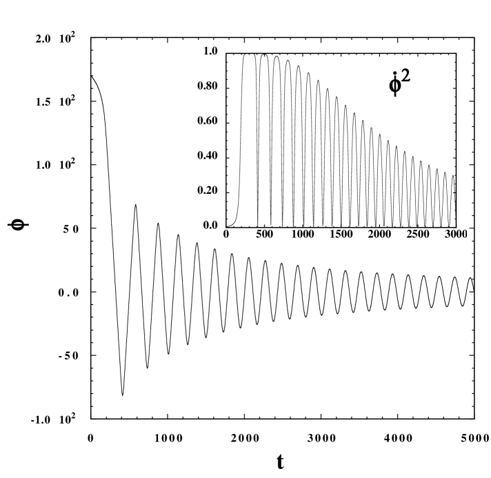
In Figs. 3 and 4 we plot the evolution of the field $\phi$ and the equation of state $w$ for the potential (26) with $\beta=10^{-3}$, $T_{3}=1$ and $\Lambda=V_{0}$. As long as $\Lambda$ is very close to $V_{0}$, the evolution of the system is very similar what is shown in Figs. 3 and 4. During the inflationary stage corresponding to $0\leq t\lesssim 200$ in the figures, $\dot{\phi}^{2}$ is much smaller than unity. This is followed by a reheating stage during which the field $\phi$ oscillates around the potential minimum. As seen from the inset of Fig. 3, $\dot{\phi}^{2}$ rapidly grows toward 1 during the transition to the reheating phase. From Fig. 4 we find that the equation of state gradually enters the region with positive $w$ during reheating. At late stage $w$ oscillates between $-1$ and $1$, which yields the average equation of state $\langle w\rangle=0$. During the initial stage of reheating $\dot{\phi}^{2}$ is close to 1, which means that the equation of state is approximately given as $w\approx-1+\dot{\phi}^{2}$ from Eq. (33). Therefore $w$ does not exceed 0 at the beginning of reheating, as seen in Fig. 4. However this picture changes with the decrease of $\dot{\phi}^{2}$ and $w$ can take positive values. When $\dot{\phi}^{2}$ becomes much smaller than 1, $w$ oscillates between $-1$ and $1$, thus yielding the equation of state for a pressure-less dust. This is similar to the standard reheating scenario with a massive inflaton KLS .

Thus our scenario provides a satisfactory equation of state during reheating unlike the case of the tachyon inflation. It was pointed out in Ref. Frolov that there is a negative instability for the tachyon fluctuations for the potential with a minimum, e.g., $V(\phi)=(1/2)m^{2}(\phi-\phi_{0})^{2}$. One may worry that this property may also hold in our scenario. However this is not the case. The each Fourier mode of the perturbation in $\phi$ satisfies the following equation on the FRW background:

$$\frac{\ddot{\delta\phi_{k}}}{1-\dot{\phi}^{2}} + \left[3H+\frac{2\dot{\phi}\ddot{\phi}}{(1-\dot{\phi}^{2})^{2}}\right]\dot{\delta\phi_{k}}$$ (69)

$$+ \left[\frac{k^{2}}{a^{2}}+(\log V),{}_{\phi\phi}\right]\delta\phi_{k}=0\,,$$

where $k$ is a comoving wavenumber. This is the generalization of the perturbation equation in Minkowski space time Frolov . While the $(\log V),{}_{\phi\phi}$ term is negative for the potential $V(\phi)=(1/2)m^{2}(\phi-\phi_{0})^{2}$, our massive rolling scalar field potential (26) corresponds to a positive mass with $(\log V),{}_{\phi\phi}=\beta m^{2}$. It is, therefore, not surprising that we do not have any instability for the perturbation $\delta\phi_{k}$ in our case. The numerical treatment of Eq.  (69) confirms this behavior of field perturbations (see Fig. 5).

Figure 5: The evolution of perturbation $\delta{\phi}_{k}$ governed by Eq. (69) for the massive Born-Infeld scalar. Unlike the case of a tachyon field, the bahavor of perturbations resembles with the evolution of $\delta{\phi}_{k}$ for an ordinary massive scalar field

This is similar to what happens in the case of the standard massive inflaton field, thus showing a viability of our scenario.

The above good behavior originates from the combination of the massive rolling scalar potential and the negative cosmological constant coming from the stabilization of the modulus. It is also possible to explain the present critical density $\rho_{c}$ when $\beta^{2}T_{3}$ is very close to $\Lambda$. Thus our scenario provides a sound mechanism to explain inflation, reheating and dark energy in the context of string theory.

VIII Conclusions and discussions

In this paper we have presented a scenario based upon a massive scalar field $\phi$ rolling on the D-brane which was shown in Ref. s2 as a possible solution in string theory. Using a DBI type effective action presented in Ref. mrg1 , we have discussed the cosmological dynamics of the rolling scalar of the anti-D3 brane of KKLT vacua, and have demonstrated that it can lead to inflationary solutions at early epochs. In our scenario it is possible to obtain a sufficient amount of inflation without tuning a fundamental string scale, unlike the case of a rolling tachyon KL . The warp metric in the KKLT vacua provides us a free parameter, the warp factor $\beta$. The presence of this parameter allows us to obtain the COBE normalized value of density perturbations without changing the brane tension and the masses of massive string states.

We further investigated scalar and tensor perturbations generated during the rolling scalar inflation and showed that our scenario is compatible with recent observational data. It is interesting to note that the steep inflation driven by an exponential potential in the Randall-Sundrum braneworld II scenario is out of the observational contour bounds cmbbrane . This is certainly related to the fact that the dynamics of the Born-Infeld scalar is very different from that of an ordinary scalar field as well as that of a scalar field on the brane.

We have also implemented the contribution of the negative cosmological constant which arises from the stabilization of the modulus fields KKLT . Although this effect is not important during inflation, the dynamics of reheating drastically changes by taking into account the negative cosmological constant that nearly cancels the potential energy of the massive rolling scalar at the potential minimum. One of the problems of the tachyon inflation is that the energy density of the tachyon scales slower than that of the pressure less matter and the radiation KL ; Frolov , which means that the tachyon over-dominates the universe after inflation. In our scenario this problem is solved by the negative cosmological constant. As shown in Sec. VII, the average equation of state of the field $\phi$ approaches that of the pressure-less dust during reheating. We also found that the negative instabity of the field fluctuations in the tachyon case Frolov is not present for the rolling massive scalar field. This suggests that the reheating proceeds in a similar way to the standard one driven by a massive inflaton field.

The massive rolling scalar can be used to explain the origin of dark energy provided that the potential energy at the minimum ($\beta^{2}T_{3}$) is very close to the amplitude of the negative cosmological constant. The presence of the negative cosmological constant is crucially important to lead to a successful reheating and to explain the origin of dark energy. Note that in the absence of the $-\Lambda$ term it is difficult to obtain the amplitude of the critical density unless we choose very small values of $\beta$.

While we performed a detailed analysis about the spectra of scalar and tensor perturbations generated in the inflationary stage, we did not precisely study the dynamics of reheating including the decay of the field $\phi$. One interesting aspect is the generation of gauge fields coupled to the rolling massive scalar as was done in Ref. jmc in the tachyon case. We leave the future work about the precise analysis of the reheating dynamics in our scenario.

References

- (1) A. Linde, Particle Physics and Inflationary Cosmology, Harwood, Chur (1990); A. R. Liddle and D. H. Lyth, Cosmological inflation and large-scale structure, Cambridge University Press (2000).
- (2) C. L. Bennett et al., Astrophys. J. Suppl. 148, 1 (2003) [arXiv:astro-ph/0302207].
- (3) D. N. Spergel et al., Astrophys. J. Suppl. 148, 175 (2003) [arXiv:astro-ph/0302209].
- (4) D. H. Lyth and A. Riotto, Phys. Rept. 314, 1 (1999) [arXiv:hep-ph/9807278].
- (5) V. Sahni and A. A. Starobinsky, Int. J. Mod. Phys. D 9, 373 (2000) [arXiv:astro-ph/9904398];T. Padmanabhan, Phys. Rept. 380, 235 (2003) [arXiv:hep-th/0212290]; B. Ratra and P. J. E. Peebles, Phys. Rev. D 37, 3406 (1988); C. Wetterich, Nucl. Phys. B 302, 668 (1988); J. A. Frieman, C. T. Hill, A. Stebbins and I. Waga, Phys. Rev. Lett. 75, 2077 (1995) [arXiv:astro-ph/9505060]; P. G. Ferreira and M. Joyce, Phys. Rev. Lett. 79, 4740 (1997) [arXiv:astro-ph/9707286]; I. Zlatev, L. M. Wang and P. J. Steinhardt, Phys. Rev. Lett. 82, 896 (1999) [arXiv:astro-ph/9807002]; P. Brax and J. Martin, Phys. Rev. D 61, 103502 (2000) [arXiv:astro-ph/9912046]; T. Barreiro, E. J. Copeland and N. J. Nunes, Phys. Rev. D 61, 127301 (2000) [arXiv:astro-ph/9910214]; A. Albrecht and C. Skordis, Phys. Rev. Lett. 84, 2076 (2000) [arXiv:astro-ph/9908085]; V. Sahni, astro-ph/0403324; D.F. Mota, C. van de Bruck, astro-ph/0401504.
- (6) P. J. Peebles and A. Vilenkin, Phys. Rev. D 59, 063505 (1999). E.J. Copeland, A. R. Liddle and J. E. Lidsey, Phys. Rev. D 64, 023509 (2001) [astro-ph/0006421]; G. Huey and Lidsey, Phys. Lett. B 514,217(2001); V. Sahni, M. Sami and T. Souradeep, Phys. Rev. D65,023518(2002); A. S. Majumdar, Phys.Rev. D64 (2001) 083503; M. Sami, N. Dadhich and Tetsuya Shiromizu, Phys.Lett. B568(2003) 118[hep-th/0304187]; M. Sami and V. Sahni, hep-th/0402086.
- (7) A. Sen, JHEP 0204, 048 (2002) [arXiv: hep-th/0203211]; JHEP 0207, 065 (2002) [ arXiv: hep-th/0203265]; Mod. Phys. Lett. A 17, 1797 (2002) [ arXiv: hep-th/0204143]; arXiv: hep-th/0312153.
- (8) A. Sen, JHEP 9910, 008 (1999) [arXiv: hep-th/9909062]; M. R. Garousi, Nucl. Phys. B584, 284 (2000) [arXiv: hep-th/0003122]; Nucl. Phys. B 647, 117 (2002) [arXiv: hep-th/0209068]; JHEP 0305, 058 (2003) [arXiv: hep-th/0304145]; E.A. Bergshoeff, M. de Roo, T.C. de Wit, E. Eyras, S. Panda, JHEP 0005, 009 (2000) [arXiv: hep-th/0003221]; J. Kluson, Phys. Rev. D 62, 126003 (2000) [arXiv: hep-th/0004106]; D. Kutasov and V. Niarchos, Nucl. Phys. B 666, 56 (2003) [arXiv: hep-th/0304045].
- (9) G. W. Gibbons, Phys. Lett. B 537, 1 (2002) [arXiv:hep-th/0204008]; M. Fairbairn and M. H. G. Tytgat, Phys. Lett. B 546, 1 (2002) [arXiv:hep-th/0204070]; S. Mukohyama, Phys. Rev. D 66, 024009 (2002) [arXiv:hep-th/0204084]; A. Feinstein, Phys. Rev. D 66, 063511 (2002) [arXiv:hep-th/0204140]; T. Padmanabhan, Phys. Rev. D 66, 021301 (2002) [arXiv:hep-th/0204150]; D. Choudhury, D. Ghoshal, D. P. Jatkar and S. Panda, Phys. Lett. B 544, 231 (2002) [arXiv:hep-th/0204204]; G. Shiu and I. Wasserman, Phys. Lett. B 541, 6 (2002) [arXiv:hep-th/0205003]; T. Padmanabhan and T. R. Choudhury, Phys. Rev. D 66, 081301 (2002) [arXiv:hep-th/0205055]; M. Sami, Mod. Phys. Lett. A 18, 691 (2003) [arXiv:hep-th/0205146]; M. Sami, P. Chingangbam and T. Qureshi, Phys. Rev. D 66, 043530 (2002) [arXiv:hep-th/0205179]. A. Ishida and S. Uehara, JHEP 0302, 050 (2003) [arXiv:hep-th/0301179]; JHEP 0210, 034 (2002) [arXiv:hep-th/0207107]; A. Mazumdar, S. Panda and A. Perez-Lorenzana, Nucl. Phys. B 614, 101 (2001) [arXiv:hep-ph/0107058]; Y. S. Piao, R. G. Cai, X. m. Zhang and Y. Z. Zhang, Phys. Rev. D 66, 121301 (2002) [arXiv:hep-ph/0207143]; Z. K. Guo, Y. S. Piao, R. G. Cai and Y. Z. Zhang, Phys. Rev. D 68, 043508 (2003) [arXiv:hep-ph/0304236]; G. N. Felder, L. Kofman and A. Starobinsky, JHEP 0209, 026 (2002) [arXiv:hep-th/0208019]; B. Wang, E. Abdalla and R. K. Su, Mod. Phys. Lett. A 18, 31 (2003) [arXiv:hep-th/0208023]; S. Mukohyama, Phys. Rev. D 66, 123512 (2002) [arXiv:hep-th/0208094]; J. g. Hao and X. z. Li, Phys. Rev. D 66, 087301 (2002) [arXiv:hep-th/0209041]; M. C. Bento, O. Bertolami and A. A. Sen, Phys. Rev. D 67, 063511 (2003) [arXiv:hep-th/0208124]; A. Sen, Int. J. Mod. Phys. A 18, 4869 (2003) [arXiv:hep-th/0209122]; C. j. Kim, H. B. Kim and Y. b. Kim, Phys. Lett. B 552, 111 (2003) [arXiv:hep-th/0210101]; J. S. Bagla, H. K. Jassal and T. Padmanabhan, Phys. Rev. D 67, 063504 (2003) [arXiv:astro-ph/0212198]; F. Leblond and A. W. Peet, JHEP 0304, 048 (2003) [arXiv:hep-th/0303035]; T. Matsuda, Phys. Rev. D 67, 083519 (2003) [arXiv:hep-ph/0302035]; A. Das and A. DeBenedictis, arXiv:gr-qc/0304017; A. DeBenedictis and A. Das, gr-qc/0207077 ; M. Majumdar and A. C. Davis, arXiv:hep-th/0304226; S. Nojiri and S. D. Odintsov, Phys. Lett. B 571, 1 (2003) [arXiv:hep-th/0306212]; D. Bazeia, F. A. Brito and J. R. S. Nascimento, Phys. Rev. D 68, 085007 (2003) [arXiv:hep-th/0306284]; L. R. W. Abramo and F. Finelli, Phys. Lett. B 575, 165 (2003) [arXiv:astro-ph/0307208]; L. Raul Abramo, Fabio Finelli, Thiago S. Pereira, astro-ph/0405041; V. Gorini, A. Y. Kamenshchik, U. Moschella and V. Pasquier, arXiv:hep-th/0311111; M. B. Causse, arXiv:astro-ph/0312206; P. K. Suresh, arXiv:gr-qc/0309043; B. C. Paul and M. Sami, arXiv:hep-th/0312081; Jian-gang Hao, Xin-zhou Li, hep-th/0303093; Xin-zhou Li, Dao-jun Liu, Jian-gang Hao, Dao-jun Liu, Xin-zhou Li, hep-th/0207146; Zong-Kuan Guo, Yuan-Zhong Zhang, hep-th/0403151; Xin-zhou Li, Jian-gang Hao, Dao-jun Liu, hep-th/0204252 ; Dao-jun Liu, Xin-zhou Li, astro-ph/0402063; J.M. Aguirregabiria, Ruth Lazkoz, hep-th/0402190; J.M. Aguirregabiria, Ruth Lazkoz, gr-qc/0402060 ; Gianluca Calcagni, hep-ph/0402126; Kenji Hotta, hep-th/0403078 ; Xin-He Meng, Peng Wang, hep-ph/0312113.
- (10) L. Kofman and A. Linde, JHEP 0207, 004 (2002) [hep-th/0205121].
- (11) A. V. Frolov, L. Kofman and A. A. Starobinsky, Phys. Lett. B 545, 8 (2002) [arXiv:hep-th/0204187].
- (12) A. Sen, JHEP 0210, 003 (2002) [arXiv:hep-th/0207105].
- (13) J. Polchinski and Y. Cai, Nucl. Phys. B 296 (1988) 91; C. G. Callan, C. Lovelace, C. R. Nappi and S. A. Yost, Nucl. Phys. B 308 (1988) 221; M. Li, Nucl. Phys. B 460 (1996) 351 [arXiv:hep-th/9510161]; O. Bergman and M. R. Gaberdiel, Nucl. Phys. B 499 183 [arXiv:hep-th/9701137].
- (14) M. B. Green and M. Gutperle, Nucl. Phys. B 476 (1996) 484 [arXiv:hep-th/9604091]; P. Di Vecchia, M. Frau, I. Pesando, A. Lerda and R. Russo, Nucl. Phys. B 507 (1997) 259 [arXiv:hep-th/9707069]; P. Di Vecchia and A. Liccardo, arXiv:hep-th/9912275.
- (15) A. Sen, JHEP 0207 (2002) 065 [arXiv:hep-th/0203265].
- (16) In spatially homogeneous field configuration, a solution is characterized by initial position and velocity of the scalar field . We choose the origin of time when velocity of the scalar field is zero. Hence, the homogeneous solution is characterized by one parameter, the initial position of scalar field.
- (17) E. Witten, Nucl. Phys. B 460, 335 (1996) [arXiv: hep-th/9510135].
- (18) N. Seiberg and E. Witten, JHEP 9909, 032 (1999) [arXiv: hep-th/9908142].
- (19) M. R. Garousi, JHEP 0312 (2003) 035 [arXiv:hep-th/0307197].
- (20) M. R. Garousi and R. C. Myers, Nucl. Phys. B 475, 193 (1996) [arXiv: hep-th/9603194]; A. Hashimoto and I. R. Klebanov, Phys. Lett. B 381, 437 (1996) [arXiv: hep-th/9604065]; Nucl. Phys. (Proc. Suppl.) B 55, 118 (1997) [arXiv: hep-th/9611214].
- (21) M. R. Garousi, JHEP 9812, 008 (1998) [arXiv: hep-th/980578]; Nucl. Phys. B 579, 209 (2000) [arXiv: hep-th/9909214].
- (22) B.S. Acharya, [arXiv: hep-th/0212294]; S. Hellerman, J. McGreevy and B. Williams, [arXiv: hep-th/0208174]; A. Dabholkar and C. Hull, [arXiv: hep-th/0210209].
- (23) S. Kachru, R. Kallosh, A. Linde and S. P. Trivedi, Phys. Rev. D 68, 046005 (2003) [arXiv: hep-th/0301240].
- (24) S. Kachru, R. Kallosh, A. Linde, J. Maldacena, L. McAllister and S. P. Trivedi, JCAP 0310, 013 (2003) [arXiv: hep-th/0308055].
- (25) R. Kallosh and A. Linde, Private communication: Throughout the paper we have assumed that the volume of internal space is frozen as in KKLT model. When inflaton field is around zero, it was shown in [23] that the non-perturbative correction (17) to the tree level superpotential makes it possible to have a positive minimum at finite volume. This is in part due to the fact that the anti-D3 brane correction (19) is small. During the inflation the anti-D3 brane correction is again like (19) in which should be replaced by . With this correction, however, one may not get anymore a local minimum for the supergravity potential during inflation in which is very large. In this case one may need to consider also corrections to the Kahler potential becker to study stabilization of the volume of internal space. In our opinion, the problem of volume stabilization in the model presented in this paper, is important and requires further investigation.
- (26) K. Becker, M. Becker, M. Haack and J. Louis, JHEP 0206, 060 (2002), [arXiv: hep-th/0204254].
- (27) K. Dasgupta, G. Rajesh and Sethi, JHEP 0008, 023 (1999) [arXiv: hep-th/9908088]; K. Becker and M. Becker, Nucl. Phys. B 477, 155 (1996) [arXiv: hep-th/9605053]; H. Verlinde, Nucl. Phys. B 580, 264 (2000) [arXiv: hep-th/9906182]; C. Chan, P. Paul and H. Verlinde, Nucl. Phys. B 581, 156 (2000) [arXiv: hep-th/0003236]; P. Mayr, Nucl. Phys. B 593, 99 (2001) [arXiv: hep-th/0003198]; JHEP 0011, 013 (2000) [arXiv: hep-th/0006204]; B. Greene, K. Schalm and G. Shiu, Nucl. Phys. B 584, 480 (2000) [arXiv: hep-th/0004103].
- (28) S. Giddings, S. Kachru and J. Polchinski, Phys. Rev. D 66, 106006 (2002) [arXiv: hep-th/0105079].
- (29) E. Witten, Nucl. Phys. B 474, 343 (1996) [arXiv: hep-th/9604030].
- (30) S. Kachru, J. Pearson and H. Verlinde, JHEP 0206, 021 (2002) [arXiv: hep-th/0112197].
- (31) G. Shiu, S.-H. H. Tye and I. Wasserman, Phys. Rev. D 67, 083517 (2003) [arXiv:hep-th/0207119]; J.M. Cline, H. Firouzjahi and P. Martineau, JHEP 12, 999 (2001) [arXiv: hep-th/0207156]; N. Barnaby and J.M. Cline, arXiv: hep-th/0403223.
- (32) J. c. Hwang and H. Noh, Phys. Rev. D 66, 084009 (2002) [arXiv:hep-th/0206100].
- (33) V. F. Mukhanov, H. A. Feldman and R. H. Brandenberger, Phys. Rept. 215, 203 (1992).
- (34) Note that in some other cosmological models can be negative. See, e.g., Ref. Shinji .
- (35) S. Tsujikawa, R. Brandenberger and F. Finelli, Phys. Rev. D 66, 083513 (2002) [arXiv:hep-th/0207228].
- (36) H. V. Peiris et al., Astrophys. J. Suppl. 148, 213 (2003) [arXiv:astro-ph/0302225]; V. Barger, H. S. Lee, and D. Marfatia, Phys. Lett. B 565, 33 (2003) [arXiv:hep-ph/0302150]; M. Tegmark et al. [SDSS Collaboration], arXiv:astro-ph/0310723.
- (37) W. H. Kinney, E. W. Kolb, A. Melchiorri, and A. Riotto, arXiv:hep-ph/0305130; S. M. Leach and A. R. Liddle, arXiv:astro-ph/0306305.
- (38) A. R. Liddle and A. J. Smith, Phys. Rev. D 68, 061301 (2003) [arXiv:astro-ph/0307017]; S. Tsujikawa and A. R. Liddle, arXiv:astro-ph/0312162.
- (39) D. A. Steer and F. Vernizzi, arXiv:hep-th/0310139.
- (40) S. Tsujikawa and B. Gumjudpai, arXiv:astro-ph/0402185, Physical Review D to appear.
- (41) J. H. Traschen and R. H. Brandenberger, Phys. Rev. D 42, 2491 (1990); Y. Shtanov, J. H. Traschen and R. H. Brandenberger, Phys. Rev. D 51, 5438 (1995); L. Kofman, A. D. Linde and A. A. Starobinsky, Phys. Rev. Lett. 73, 3195 (1994); Phys. Rev. D 56, 3258 (1997).