Glueball Scattering Amplitudes from Holography

Abstract:

Using techniques developed in a previous paper three-point functions in field theories described by holographic renormalization group flows are computed. We consider a system of one active scalar and one inert scalar coupled to gravity. For the GPPZ flow, their dual operators create states that are interpreted as glueballs of the $\mathcal{N}=1$ SYM theory, which lies at the infrared end of the renormalization group flow. The scattering amplitudes for three-glueball processes are calculated providing precise predictions for glueball decays in $\mathcal{N}=1$ SYM theory. Numerical results for low-lying glueballs are included.

1 Introduction

It is a paradigm of the AdS/CFT correspondence that the dynamics of a field theory living in an (asymptotically) anti-de Sitter bulk space-time encodes the correlation functions of its dual (deformed) conformal field theory [1, 2]. The correspondence holds par excellence for $\mathcal{N}=8$ gauged supergravity in $(d+1)=5$ dimensions on the bulk side, which is obtained from $D=10$ type IIB supergravity by compactification on a five-sphere. Its $AdS_{5}$ solution is dual, in the planar limit and at strong ’t Hooft coupling, to $d=4$, $\mathcal{N}=4$ super Yang-Mills (SYM) theory, which is a conformal quantum field theory [3].

The study of fluctuations around other bulk configurations, which are interpreted as the duals of Renormalization Group (RG) flows of $\mathcal{N}=4$ SYM theory driven by relevant operators, is interesting, because it yields the correlation functions of the respective dual quantum field theories in a regime that is not accessible by ordinary perturbation theory. For example, the GPPZ flow [4], which is a supersymmetric mass deformation of $\mathcal{N}=4$ SYM theory, possesses many qualitative features of pure $\mathcal{N}=1$ SYM theory, in particular quark confinement. The two-point functions in the GPPZ flow, which have been calculated using holography, exhibit a spectrum of particles, which must arise from as yet unknown non-perturbative effects in the field theory. These particles are interpreted as glueballs of the $\mathcal{N}=1$ SYM theory, which lies at the infra-red end of the RG flow [6]. Naturally, a calculation of the glueball scattering amplitudes would be very desirable.

Until recently, the holographic calculation of $n$-point functions with $n>2$ involving the operators that are dual to the active scalars of holographic RG flow backgrounds was considered unfeasible, because their fluctuations couple to the fluctuations of the bulk metric even at the linearized level. In contrast, inert scalars do not couple to the bulk metric at the linearized level, and the calculation of the corresponding three-point functions is rather straightforward [7]. In a recent paper [8], however, enormous progress was made exploiting a gauge invariant formalism, in which the true degrees of freedom of the bulk metric decouple from the active scalar fluctuations at the linearized level. Thus, this formalism simplifies the calculations of two-point functions for the active scalars and makes higher $n$-point functions accessible by the use of the Green’s function method. This was demonstrated for the case of a single active scalar, which is dual to an operator $\mathcal{O}$, by calculating the three-point function $\left\langle\mathcal{O}\mathcal{O}\mathcal{O}\right\rangle$. An important result of [8] was the proof of Bose symmetry, which was not obvious from the formal expression resulting from the Green’s function method. This proof involved two steps, which we shall summarize here. In the first step a field redefinition was used in order to eliminate those terms from the quadratic source of the field equations that contain two radial derivatives. Then, after using momentum conservation, some terms in the radial integral were integrated by parts, and the final, Bose symmetric result was obtained. Moreover, it was shown (for the GPPZ flow) that the boundary terms from the integration by parts cancel the contribution from the field redefinition.

In this paper, we continue the programme of [8] considering a system of one active and one inert scalar coupled to bulk gravity in a generic holographic RG flow background and finding the expressions for all non-local three-point functions of the respective dual operators. Applied to the GPPZ flow, the results are then used to calculate the scattering amplitudes for the glueballs generated by these operators. Thus, for the first time, we are able to predict glueball scattering amplitudes for an $\mathcal{N}=1$ SYM theory using holography.

In order to avoid being repetitive we chose not to draft this paper in a self-contained fashion, but to make essential use of the material presented in [8]. Hence, we urge the reader to consult that paper first in order to become familiar with the gauge invariant method and our notation. We also refer to [8] for more references to the relevant literature.

The rest of this paper is organized as follows. In Sec. 2 we review the equations of motion using the gauge invariant formalism developed in [8]. Sec. 3, which contains the main achievements of our work, is devoted to the study of three-point functions in a generic holographic RG flow background containing one active and one inert scalar field. Together with the bulk graviton, the three respective dual boundary operators give rise to a total of ten independent three-point functions, all of which will be calculated. We proceed as in [8] performing first a field redefinition and then a suitable integration by parts in order to render the final results Bose symmetric. However, we shall not be concerned about whether the boundary terms resulting from the two steps cancel each other, as the net boundary terms would contribute only contact terms to the three-point functions. Our final expressions for the three-point functions have the form of generically divergent integrals. The divergences, which have the form of contact terms, can be easily understood and removed on a case-by-case basis by comparison with the results of holographic renormalization, and, thus, we shall not do it explicitly for the general setup. Such an attitude is justified, because contact terms have no effect on the scattering amplitudes.

As an application of our results of Sec. 3 we shall analyze the GPPZ flow in Secs. 4 and 5. In Sec. 4, we start by repeating the analysis of the bulk-to-boundary propagators, which give rise to the two-point functions. Then, we shall present the expressions that encode the non-local three-point functions and scattering amplitudes. Moreover, we shall illustrate how the divergences of the three-point function integrals are understood and removed by using holographic renormalization. Finally, in Sec. 5, we discuss some physical interpretations of the calculated scattering amplitudes, in particular the possible glueball decay channels. Some useful relations for the GPPZ flow can be found in appendix A, and numerical results for the decay amplitudes are listed in appendix B.

Let us stress that we are interested only in the non-local three-point functions. A detailed analysis of the contact terms would be a worthwhile exercise, because they play a crucial role in the consistency of the subtraction procedure [10] and contribute to certain sum rules [11]. Such an analysis would have to take into account not only the contact terms that result from holographic renormalization [12, 10, 13], but also the use of the gauge invariant fields, the field redefinition and the integration by parts, which occur in our calculation. In particular, analyzing the contributions from the use of the gauge invariant fields might be rather challenging, because one would need to translate the fields into the axial gauge, in which holographic renormalization has been carried out. Moreover, this translation must be done to third order in the fluctuations (to obtain all local terms in the three-point functions), but we have only derived the linear relations, which are sufficient for the analysis of the bulk equations of motion. Alternatively, one might try to perform holographic renormalization in a gauge invariant fashion. However, contact terms can be calculated only on a case-by-case basis, e.g., for the GPPZ flow. Thus, it would be impossible to include them into our general results of Sec. 3. Having in mind to calculate the scattering amplitudes for on-shell glueballs in the GPPZ flow, we feel justified in omitting them completely.

2 Field Equations

In this section, we shall present the equations of motion to quadratic order in the fluctuations for a bulk system containing one active scalar, $\phi$, and one inert scalar, $\sigma$, coupled to gravity. Our main reason for this restriction of the number of scalars is that, generically, it is impossible to diagonalize the effective mass terms of scalars of the same kind (active or inert) in holographic RG flow backgrounds. Thus, we ensure that the linear second order ODEs for the true degrees of freedom are not coupled, which makes the use of the Green’s function method straightforward. Our results are easily generalized to the case of several inert scalars with diagonal effective mass terms.

The equations of motion shall be presented in the gauge invariant approach of [8]. In this approach, the field fluctuations are combined into a set of gauge invariant variables, in terms of which the equations of motion are expressed. The remaining fluctuations describe gauge artifacts and are explicitly dropped.

For completeness, we shall review in subsection 2.1 the general relations defining a holographic RG flow background and the definitions of the gauge invariant variables. Then, in subsections 2.2, 2.3 and 2.4, respectively, the equations of motion for the active scalar, the inert scalar and the traceless transversal parts of the bulk metric fluctuations are presented.

2.1 Preliminaries

A generic holographic RG flow background with one active scalar satisfies [14, 15, 16]

$$\begin{split}\mathrm{d}s^{2}&=\mathrm{d}r^{2}+\mathrm{e}^{2A(r)}\eta_{ij}\mathrm{d}x^{i}\mathrm{d}x^{j}~{},\\ \partial_{r}A(r)&=-\frac{2}{d-1}W(\bar{\phi})~{},\\ \partial_{r}\bar{\phi}&=W_{\phi}(\bar{\phi})~{},\quad\bar{\sigma}=0~{},\end{split}$$ (1)

where the superpotential $W$ is a function of the active scalar and satisfies the following functional equation, which is imposed by the supersymmetry of the background,

$$\frac{1}{2}W_{\phi}^{2}-\frac{d}{d-1}W^{2}=V|_{\sigma=0}~{}.$$ (2)

Here and henceforth, derivatives with respect to the fields are denoted by subscripts, as in $W_{\phi}=\mathrm{d}W/\mathrm{d}\phi$. Notice that, in general, (2) does not include the inert scalar, although in some cases (e.g., for the GPPZ flow) it might be possible that the full potential $V$ is expressible in terms of a suitable superpotential containing also the inert scalar.

The couplings between the inert scalar and the active scalar are strongly restricted by the fact that the relation $V_{\sigma}=\partial V/\partial\sigma=0$ holds in the background due to the equation of motion for $\sigma$. Taking a derivative of this relation with respect to $r$ we find

$$0=\partial_{r}V_{\sigma}=V_{\sigma\phi}W_{\phi}~{},$$ (3)

so that we find also $V_{\sigma\phi}=0$. Applying this argument recursively one arrives at the conclusion that

$$V_{\sigma\phi\cdots\phi}=0$$ (4)

for any number of $\phi$-derivatives. Notice that this argument does not hold in the more general case with several active scalars. In that case the right hand side of (3) contains a sum over all active scalars, and the members of the sum need not be zero individually.

We shall now review the definition of the gauge invariant variables. The bulk system is treated in the time slicing formalism, where the bulk metric is written in the form

$$\mathrm{d}s^{2}=(n^{2}+n_{i}n^{i})\mathrm{d}r^{2}+2n_{i}\mathrm{d}r\mathrm{d}x^{i}+g_{ij}\mathrm{d}x^{i}\mathrm{d}x^{j}~{}.$$ (5)

The fluctuations of the various fields around the background (1) are introduced by

$$\phi =\bar{\phi}(r)+\varphi~{},\qquad \sigma =\sigma,$$ (6)

$$n_{i} =\nu_{i}~{}, n =1+\nu~{},$$

$$g_{ij} =\mathrm{e}^{2A(r)}\left(\eta_{ij}+h_{ij}\right)~{}.$$

Furthermore, the metric fluctuations $h^{i}_{j}$ are split as follows,

$$h^{i}_{j}={h^{TT}}^{i}_{j}+\partial^{i}\epsilon_{j}+\partial_{j}\epsilon^{i}+\frac{\partial^{i}\partial_{j}}{\Box}H+\frac{1}{d-1}\delta^{i}_{j}h~{},$$ (7)

where ${h^{TT}}^{i}_{j}$ denotes the traceless transversal part, and $\epsilon^{i}$ is a transversal vector ($\partial_{i}\epsilon^{i}=0$).

The inert scalar, $\sigma$, is gauge invariant to lowest order. Therefore, we shall use the same symbol to denote the corresponding (all order) gauge invariant variable. The remaining first-order gauge invariant combinations of the fluctuations are

$$a =\varphi+W_{\phi}\frac{h}{4W}~{},$$ (8)

$$b =\nu+\partial_{r}\left(\frac{h}{4W}\right)~{},$$ (9)

$$c =\partial_{i}\nu^{i}+\Box\frac{h}{4W}-\frac{1}{2}\mathrm{e}^{2A}\partial_{r}H~{},$$ (10)

$$d^{i} =\Pi^{i}_{j}\nu^{j}-\mathrm{e}^{2A}\partial_{r}\epsilon^{i}~{},\phantom{\frac{1}{2}}$$ (11)

$$e^{i}_{j} =h^{TT}{}^{i}_{j}=\Pi^{ik}_{jl}h^{l}_{k}~{}.$$ (12)

Here and henceforth, $\Pi^{i}_{j}$ and $\Pi^{ik}_{jl}$ denote the transversal and the traceless transversal projectors, respectively,

$$\Pi^{i}_{j} =\delta^{i}_{j}-\frac{\partial^{i}\partial_{j}}{\Box}~{},$$ (13)

$$\Pi^{ik}_{jl} =\frac{1}{2}\left(\Pi^{ik}\Pi_{jl}+\Pi^{i}_{l}\Pi^{k}_{j}\right)-\frac{1}{d-1}\Pi^{i}_{j}\Pi^{k}_{l}~{}.$$ (14)

The gauge invariant approach is embodied in a simple recipe, according to which one expands the field equations to the desired order and replaces the fluctuations as follows,

$$\varphi\to a~{},\quad\nu\to b~{},\quad\nu^{i}\to d^{i}+\frac{\partial^{i}c}{\Box}~{},\quad h^{i}_{j}\to e^{i}_{j}~{}.$$ (15)

The fluctuations $\epsilon^{i}$, $h$ and $H$ represent gauge artifacts and are explicitly dropped, while the inert scalar $\sigma$ remains unchanged.

Finally we mention that, as in [8], we raise and lower the indices of fluctuations and of partial derivatives using the flat metric.

2.2 The Equation for the Active Scalar

The equations of motion for the active scalar can be taken over from Sec. 4 of [8] with only minor modifications, which come in the form of additional terms that are quadratic in the inert scalar. Terms with only one $\sigma$ cannot occur because of (4). For completeness, we repeat the full expressions here. First, the scalar equation remains

$$\left(\partial_{r}^{2}-\frac{2d}{d-1}W\partial_{r}+\mathrm{e}^{-2A}\Box-V_{\phi\phi}\right)a-W_{\phi}\mathrm{e}^{-2A}c-W_{\phi}\partial_{r}b-2V_{\phi}b=J_{a}~{},$$ (16)

where the source $J_{a}$ is now given by

$$\begin{split}J_{a}&=\frac{1}{2}V_{\phi\phi\phi}a^{2}+V_{\phi}b^{2}+2V_{\phi\phi}ab-W_{\phi}b\partial_{r}b+(\partial_{r}a)(\partial_{r}b)+\frac{1}{2}W_{\phi}e^{i}_{j}\partial_{r}e^{j}_{i}\\ &\quad+\mathrm{e}^{-2A}\left[-2b\Box a-(\partial^{i}b)(\partial_{i}a)+c\partial_{r}a+2\left(d^{i}+\frac{\partial^{i}c}{\Box}\right)\partial_{i}\partial_{r}a\right.\\ &\quad-W_{\phi}\left(d^{i}+\frac{\partial^{i}c}{\Box}\right)\partial_{i}b+\left(\partial_{r}d^{i}+\partial_{r}\frac{\partial^{i}c}{\Box}\right)\partial_{i}a-2\frac{d-2}{d-1}W\left(d^{i}+\frac{\partial^{i}c}{\Box}\right)\partial_{i}a\\ &\left.\phantom{\frac{1}{2}}+e^{i}_{j}\left(\partial_{i}\partial^{j}a-W_{\phi}\partial_{i}d^{j}-W_{\phi}\frac{\partial_{i}\partial^{j}}{\Box}c\right)\right]+\frac{1}{2}V_{\phi\sigma\sigma}\sigma^{2}~{}.\end{split}$$ (17)

Second, the normal component of Einstein’s equation is

$$-4W\mathrm{e}^{-2A}c+4W_{\phi}\partial_{r}a-4V_{\phi}a-8Vb=J_{c}~{},$$ (18)

where the source $J_{c}$ is easily generalized from (4.6) of [8],

$$\begin{split}J_{c}&=4Vb^{2}+8V_{\phi}ab+2V_{\phi\phi}a^{2}-2(\partial_{r}a)^{2}+(\mathrm{e}^{-2A}c)^{2}+2\mathrm{e}^{-2A}(\partial^{i}a)(\partial_{i}a)\\ &\quad+4W_{\phi}\mathrm{e}^{-2A}\left(d^{i}+\frac{\partial^{i}c}{\Box}\right)\partial_{i}a+2We^{i}_{j}\partial_{r}e^{j}_{i}-4W\mathrm{e}^{-2A}e^{i}_{j}\partial_{i}\left(d^{j}+\frac{\partial^{j}c}{\Box}\right)\\ &\quad-\frac{1}{4}(\partial_{r}e^{i}_{j})(\partial_{r}e^{j}_{i})+\mathrm{e}^{-2A}\left(\partial_{i}d^{j}+\frac{\partial_{i}\partial^{j}}{\Box}c\right)\partial_{r}e^{i}_{j}\\ &\quad-\mathrm{e}^{-4A}\left[\frac{1}{2}(\partial_{i}d^{j})(\partial^{i}d_{j})+\frac{1}{2}(\partial_{i}d^{j})(\partial_{j}d^{i})+2(\partial_{i}d^{j})\frac{\partial^{i}\partial_{j}}{\Box}c+\left(\frac{\partial_{i}\partial^{j}}{\Box}c\right)\left(\frac{\partial^{i}\partial_{j}}{\Box}c\right)\right]\\ &\quad-\mathrm{e}^{-2A}\left[e^{i}_{j}\Box e^{j}_{i}+\frac{3}{4}(\partial_{i}e^{j}_{k})(\partial^{i}e_{j}^{k})-\frac{1}{2}(\partial_{i}e^{j}_{k})(\partial^{k}e^{i}_{j})\right]\\ &\quad+2V_{\sigma\sigma}\sigma^{2}-2(\partial_{r}\sigma)(\partial_{r}\sigma)+2\mathrm{e}^{-2A}(\partial^{i}\sigma)(\partial_{i}\sigma)~{}.\end{split}$$ (19)

Third, the mixed components of Einstein’s equation yield

$$-\frac{1}{2}\mathrm{e}^{-2A}\Box d_{i}-2W\partial_{i}b-2W_{\phi}\partial_{i}a=J_{i}~{},$$ (20)

and the source $J_{i}$ now is

$$\begin{split}J_{i}&=-W\partial_{i}b^{2}+2(\partial_{i}a)(\partial_{r}a)+\mathrm{e}^{-2A}(\Pi^{j}_{i}c)(\partial_{j}b)+\frac{1}{2}(\partial_{j}b)(\partial_{r}e^{j}_{i})-\frac{1}{2}\mathrm{e}^{-2A}\frac{\partial_{j}c}{\Box}\Box e^{j}_{i}\\ &\quad-\frac{1}{4}\partial_{i}\partial_{r}(e^{j}_{k}e^{k}_{j})+\frac{1}{2}e^{j}_{k}\partial_{r}\partial_{j}e^{k}_{i}+\frac{1}{4}(\partial_{i}e^{j}_{k})(\partial_{r}e^{k}_{j})-\frac{1}{2}\mathrm{e}^{-2A}e^{j}_{k}\partial_{j}(\partial^{k}d_{i}-\partial_{i}d^{k})\\ &\quad-\frac{1}{2}\mathrm{e}^{-2A}(\partial_{j}e^{k}_{i})(\partial^{j}d_{k}-\partial_{k}d^{j})-\frac{1}{2}\mathrm{e}^{-2A}d_{j}\Box e^{j}_{i}-\frac{1}{2}\mathrm{e}^{-2A}(\partial_{j}b)(\partial^{j}d_{i}+\partial_{i}d^{j})\\ &\quad+2(\partial_{i}\sigma)(\partial_{r}\sigma)~{}.\end{split}$$ (21)

As in [8], we first define $\tilde{a}=(W/W_{\phi})a$ and solve (18) and (20) for $b$, $c$ and $d_{i}$, with the results

$$\begin{split}b&=-\frac{W_{\phi}^{2}}{W^{2}}\tilde{a}-\frac{1}{2W}\frac{\partial_{i}}{\Box}J^{i}~{},\\ \Box d_{i}&=-2\mathrm{e}^{2A}\Pi^{j}_{i}J_{j}~{},\\ \mathrm{e}^{-2A}c&=\frac{W_{\phi}^{2}}{W^{2}}\partial_{r}\tilde{a}-\frac{1}{4W}J_{c}+\frac{V}{W^{2}}\frac{\partial_{i}}{\Box}J^{i}~{}.\end{split}$$ (22)

Then, we substitute (22) into (16), which yields the following second order ODE for $\tilde{a}$,

$$\left(D^{2}+\mathrm{e}^{-2A}\Box\right)\tilde{a}=J_{\tilde{a}}~{}.$$ (23)

We have abbreviated

$$D^{2}=\left[\partial_{r}+2\left(W_{\phi\phi}-\frac{W_{\phi}^{2}}{W}-\frac{d}{d-1}W\right)\right]\partial_{r}~{},$$ (24)

and the source term in (23) is given by

$$J_{\tilde{a}}=\frac{W}{W_{\phi}}J_{a}-\frac{1}{4}J_{c}-\frac{1}{2}\left[\partial_{r}+2\left(W_{\phi\phi}-\frac{W_{\phi}^{2}}{W}-\frac{d}{d-1}W\right)\right]\frac{\partial_{i}}{\Box}J^{i}~{}.$$ (25)

In the source (25), the first order terms of the solutions (22) should be substituted.

2.3 The Equation for the Inert Scalar

The equation for the inert scalar is quite easily obtained from (16) and (17) by dropping the terms with $W_{\phi}$ and $V_{\phi}$ and generalizing the derivatives of $V$. One obtains

$$\left(\partial_{r}^{2}-\frac{2d}{d-1}W\partial_{r}+\mathrm{e}^{-2A}\Box-V_{\sigma\sigma}\right)\sigma=J_{\sigma}~{},$$ (26)

where the source $J_{\sigma}$ is

$$\begin{split}J_{\sigma}&=\frac{1}{2}V_{\sigma\sigma\sigma}\sigma^{2}+V_{\sigma\sigma\phi}\sigma a+2V_{\sigma\sigma}\sigma b+(\partial_{r}\sigma)(\partial_{r}b)\\ &\quad+\mathrm{e}^{-2A}\left[-2b\Box\sigma-(\partial^{i}b)(\partial_{i}\sigma)+c\partial_{r}\sigma+2\left(d^{i}+\frac{\partial^{i}c}{\Box}\right)\partial_{i}\partial_{r}\sigma\right.\\ &\left.\quad+\left(\partial_{r}d^{i}+\partial_{r}\frac{\partial^{i}c}{\Box}\right)\partial_{i}\sigma-2\frac{d-2}{d-1}W\left(d^{i}+\frac{\partial^{i}c}{\Box}\right)\partial_{i}\sigma+e^{i}_{j}\partial_{i}\partial^{j}\sigma\right]~{}.\end{split}$$ (27)

2.4 The Equation for the Graviton

The tangential components of Einstein’s equation provide the equations of motion for the traceless transversal modes $e^{i}_{j}$. Following the notation of [8], we first write these components in terms of time-slice hyper surface quantities, which gives

$$-\partial_{r}(n\mathcal{K}^{i}_{j})+n^{k}\nabla_{k}(n\mathcal{K}^{i}_{j})+(n\mathcal{K}^{i}_{j})(n\mathcal{K}^{k}_{k}+\partial_{r}\ln n-n^{k}\partial_{k}\ln n)\\ +n\nabla^{i}\partial_{j}n+(n\mathcal{K}^{i}_{k})\nabla_{j}n^{k}-(n\mathcal{K}^{k}_{j})\nabla_{k}n^{i}+n^{2}R^{i}_{j}+2n^{2}S^{i}_{j}=0~{},$$ (28)

where

$$S^{i}_{j}=g^{ik}\left(\partial_{k}\phi\partial_{j}\phi+\partial_{k}\sigma\partial_{j}\sigma\right)+\frac{2}{d-1}\delta^{i}_{j}V(\phi,\sigma)~{}.$$ (29)

In order to obtain an equation containing only the gauge invariants $e^{i}_{j}$, $\tilde{a}$ and $\sigma$, we should expand (28) to second order and substitute the solutions (22) for $b$, $c$ and $d^{i}$. However, it is clear that the trace and the divergence of the resulting equation would both vanish by virtue of the equation for $\tilde{a}$, (23), because the scalar equation is implied by Einstein’s equation via the Bianchi identity. Thus, we can project onto the traceless transversal components using the projector (14) in order to find the only independent equation that is still missing. The result is

$$\left(\partial_{r}^{2}-\frac{2d}{d-1}W\partial_{r}+\mathrm{e}^{-2A}\Box\right)e^{i}_{j}=J^{i}_{j}~{},$$ (30)

where the quadratic source terms are given by

$$\begin{split}J^{i}_{j}&=\Pi^{ik}_{jl}\left\{(\partial_{r}e^{l}_{m})(\partial_{r}e^{m}_{k})-\mathrm{e}^{-2A}\left[e^{m}_{n}(2\partial^{l}\partial_{m}e^{n}_{k}-\partial_{m}\partial^{n}e^{l}_{k})\phantom{\frac{1}{2}}\right.\phantom{\left(\left(\frac{1}{2}\right)^{2}\right)}\right.\\ &\quad\left.+\frac{1}{2}(\partial^{l}e^{m}_{n})(\partial_{k}e^{n}_{m})+(\partial_{m}e^{l}_{n})(\partial^{n}e^{m}_{k})-(\partial_{m}e^{n}_{k})(\partial^{m}e^{l}_{n})\right]\\ &\quad+2\left(\frac{W_{\phi}}{W}\right)^{2}\left[(\partial_{m}\partial_{r}e^{l}_{k})\left(\frac{\partial^{m}}{\Box}\partial_{r}\tilde{a}\right)+\mathrm{e}^{-2A}\tilde{a}\Box e^{l}_{k}\right]-\left[\partial_{r}\left(\frac{W_{\phi}}{W}\right)^{2}\right]\tilde{a}\partial_{r}e^{l}_{k}\\ &\quad+2\left(\frac{W_{\phi}}{W}\right)^{4}\left[\left(\frac{\partial^{l}\partial_{m}}{\Box}\partial_{r}\tilde{a}\right)\left(\frac{\partial^{m}\partial_{k}}{\Box}\partial_{r}\tilde{a}\right)+\mathrm{e}^{-2A}\partial^{l}\tilde{a}\partial_{k}\tilde{a}\right]\\ &\quad\left.+\left[\partial_{r}\left(\frac{W_{\phi}}{W}\right)^{4}\right]\tilde{a}\frac{\partial^{l}\partial_{k}}{\Box}\partial_{r}\tilde{a}-4\mathrm{e}^{-2A}\left[\left(\frac{W_{\phi}}{W}\right)^{2}\partial^{l}\tilde{a}\partial_{k}\tilde{a}+\partial^{l}\sigma\partial_{k}\sigma\right]\right\}~{}.\end{split}$$ (31)

3 Three-Point Functions

3.1 General Form

The dynamics of the bulk fields, which is governed by the equations presented in the previous section, encodes the two- and three-point functions of the dual operators. For completeness and in order to outline our conventions for the presentation of the final results, we shall in the following review how the correlations functions are obtained from the (sub-leading) asymptotic behaviour of the bulk fields.

The gauge invariant fields $a$, $\sigma$ and $e^{i}_{j}$, which are the true degrees of freedom of our bulk system, are dual to the operators $\mathcal{O}$, $\Sigma$ and $T^{i}_{j}$, respectively. Here and henceforth, we denote by $T^{i}_{j}$ the traceless transversal part of the boundary energy-momentum tensor,

$$T^{i}_{j}=\Pi^{ik}_{jl}\Theta^{l}_{k}~{}.$$ (32)

The duality between the bulk fields and the boundary operators is made explicit through the couplings

$$\int\mathrm{d}^{d}x\,\left[\hat{a}(x)\mathcal{O}(x)+\hat{\sigma}(x)\Sigma(x)+\frac{1}{2}\hat{e}^{i}_{j}(x)T^{j}_{i}(x)\right]~{},$$ (33)

where $\hat{a}$, $\hat{\sigma}$ and $\hat{e}^{i}_{j}$ are the prescribed asymptotic boundary values of the bulk fields $a$, $\sigma$ and $e^{i}_{j}$, respectively.

The other components of the energy momentum tensor are not independent, because the (anomalous) Ward identities [10, 13] imply the operator identities

$$\partial_{i}\Theta^{i}_{j}=0~{},\quad\Theta=\beta\mathcal{O}~{},$$ (34)

which are valid in all correlation functions with distinct insertion points. For vev flows we have $\beta=0$, whereas in operator flows $\beta=-(d-\Delta)\hat{\bar{\phi}}$, where $\Delta$ is the conformal dimension of $\mathcal{O}$ at the ultraviolet conformal fixed point of the RG flow.

In order to start, let us denote by $\psi$ a generic bulk field. Its behaviour in the asymptotically AdS region of the bulk space-time is described by the generic expansion

$$\psi(\rho,x)=\rho^{(d-\Delta)/2}[\hat{\psi}(x)+\cdots]+\rho^{\Delta/2}[\check{\psi}(x)+\cdots]~{}.$$ (35)

Throughout this section, we shall use the variable $\rho=\mathrm{e}^{-2r}$, so that the asymptotic region is given by $\rho\to 0$. Here, $\Delta$ denotes the conformal dimension of the operator dual to $\psi$, which we shall call $\Psi$. The ellipses in (35) stand for the sub-leading terms in the two series, which are power series in $\rho$, whose coefficients depend locally on $\hat{\psi}$ and $\check{\psi}$, respectively. If $\Delta-d/2$ is an integer, the leading series contains also logarithms. The function $\check{\psi}$ is called the response function, and its non-trivial dependence on the source $\hat{\psi}$ stems from the condition of regularity of $\psi$ in the bulk interior. Moreover, the response function $\check{\psi}$ determines the exact one-point function of the operator $\Psi$. More precisely, we have [12, 10, 13]

$$\left\langle\Psi\right\rangle=(2\Delta-d)\check{\psi}+\text{contact terms}~{},$$ (36)

where the contact terms are finite, but in principle scheme dependent. We shall not be concerned with the contact terms in this paper. A slightly different version of (36) is needed for the exact one-point function $\left\langle T^{i}_{j}\right\rangle$, which is

$$\left\langle T^{i}_{j}\right\rangle=\frac{1}{4}(2\Delta-d)\check{e}^{i}_{j}=\frac{d}{4}\check{e}^{i}_{j}~{}.$$ (37)

Here, contact terms have been omitted. The factor $1/4$ stems from the $1/4$ in front of the Einstein-Hilbert term in the bulk action in our conventions [8].

Let us focus our attention now on the response function, $\check{\psi}$. In order to determine it we first observe that $\psi$ satisfies a second order ODE of the form

$$\left(\tilde{\nabla}^{2}-M^{2}\right)\psi=J_{\psi}~{},$$ (38)

where $M^{2}$ is an effective mass term, $\tilde{\nabla}$ denotes the background covariant derivative, and $J_{\psi}$ is a higher order source term. Thus, after defining a covariant Green’s function by

$$\left(\tilde{\nabla}^{2}-M^{2}\right)G(z,z^{\prime})=\frac{\delta(z-z^{\prime})}{\sqrt{\tilde{g}(z)}}~{},$$ (39)

the general solution of (38) is given by

$$\psi(z)=\int\mathrm{d}^{d}y\,K(z,y)\hat{\psi}(y)+\int\mathrm{d}^{d+1}z^{\prime}\,\sqrt{\tilde{g}(z^{\prime})}G(z,z^{\prime})J_{\psi}(z^{\prime})~{}.$$ (40)

Here, $z$ is a short notation for the variables $(\rho,x)$, and $x$ and $y$ are boundary coordinates. Notice that the bulk integral is cut off at $\rho^{\prime}=\varepsilon$, and also that $\rho\geq\varepsilon$, because of the regularization procedure. Moreover, $K(z,y)$ denotes the bulk-to-boundary propagator of the field $\psi$.

We are interested in the near-boundary behaviour of $\psi$, and it is very helpful that in asymptotically AdS spaces the Green’s function asymptotically behaves as [19]

$$G(z,z^{\prime})\approx-\frac{\rho^{\Delta/2}}{2\Delta-d}K(x,z^{\prime})+\cdots~{}.$$ (41)

Hence, let us consider the field at the cut-off boundary by setting $\rho=\epsilon$, and let us switch to momentum space, where we can use momentum conservation of the propagators, $K(\rho,p;q)=K_{p}(\rho)\delta(p+q)$. Then, (40) leads to

$$\psi(\varepsilon,p)\approx K_{p}(\varepsilon)\hat{\psi}(p)-\frac{\varepsilon^{\Delta/2}}{2\Delta-d}\int\limits_{\varepsilon}\frac{\mathrm{d}\rho}{2\rho}\mathrm{e}^{dA(\rho)}K_{p}(\rho)J_{\psi}(\rho,p)~{}.$$ (42)

From this general expression one must extract the response function $\check{\psi}$, which represents, by virtue of (36), the exact one-point function of the dual operator $\Psi$. The two-point function $\left\langle\Psi\Psi\right\rangle$ can be read off easily from the asymptotic behaviour of the bulk-to-boundary propagator $K_{p}$.

The various three-point functions that contain $\Psi$ are obtained from the interaction integral in (42). In order to be more explicit, let us consider a generic three-point function $\left\langle\Psi_{1}\Psi_{2}\Psi_{3}\right\rangle$, where the $\Psi_{n}$, $n=1,2,3$, can be identical or different. Their respective dependence on the momenta $p_{n}$ is implied. This three-point function can be obtained from the integral in (42) setting, e.g., $\psi=\psi_{1}$. The term in $J_{\psi_{1}}$ that is responsible for the three-point functions $\left\langle\Psi_{1}\Psi_{2}\Psi_{3}\right\rangle$ has the generic form

$$J_{\psi_{1}}(\rho,p_{1})=\int\mathrm{d}p_{2}\,\mathrm{d}p_{3}\,\delta(p_{1}+p_{2}+p_{3})\mathcal{X}(p_{1},-p_{2},-p_{3})K_{2}(\rho)K_{3}(\rho)\hat{\psi}_{2}(-p_{2})\hat{\psi}_{3}(-p_{3})~{},$$ (43)

where we have substituted the linear solutions for the bulk fields $\psi_{2}$ and $\psi_{3}$, and $\mathcal{X}$ is an operator containing also derivatives with respect to $\rho$ (or, equivalently, $r$) acting on the bulk-to-boundary propagators $K_{2}$ and $K_{3}$. It is also important to notice the minus signs in front of $p_{2}$ and $p_{3}$. Differentiating (43) with respect to the sources $\hat{\psi}_{2}$ and $\hat{\psi}_{3}$ and substituting the result into (42) yields the three-point function of the form

$$\left\langle\Psi_{1}\Psi_{2}\Psi_{3}\right\rangle=-\delta(p_{1}+p_{2}+p_{3})\int\mathrm{d}r\,\mathrm{e}^{dA}\left(\frac{W_{\phi}}{W}\right)^{2}\mathcal{X}_{123}K_{1}K_{2}K_{3}~{},$$ (44)

where $\mathcal{X}_{123}$ is again an operator acting on the bulk-to-boundary propagators, which can be obtained easily from the source $J_{\psi_{1}}$.

Eqn. (44) is the general expression for the three-point functions, and our main work will consist in calculating the operators $\mathcal{X}_{123}$. To explain this formula more precisely several clarifications are in order. First, the factor $(W_{\phi}/W)^{2}$ has been inserted for continuity with our previous calculations in [8], where it automatically appeared when using the field $\tilde{a}$ and its corresponding bulk-to-boundary propagator, $\tilde{K}$. In fact, in the case $\Psi_{1}=\mathcal{O}$, the operator $\mathcal{X}_{123}$ can be read off directly from the source $J_{\tilde{a}}$. In the other cases, $\Psi_{1}=\Sigma$ and $\Psi_{1}=T^{i}_{j}$, we must multiply a factor $(W_{\phi}/W)^{-2}$ to the operators read off from $J_{\sigma}$ and $J^{i}_{j}$, respectively, in order to compensate for the factor in (44). Second, we must correctly carry out the functional derivatives with respect to the sources, if $\Psi_{2}$ and $\Psi_{3}$ are identical, which symmetrizes the operator of interest with respect to the indices 2 and 3. Third, because of (33) and (37), we must include a factor $1/4$, if $\Psi_{1}=T^{i}_{j}$, and a factor $2$ for each $T^{i}_{j}$ at the positions $2$ and $3$. Forth, the reader is reminded of the minus signs in front of $p_{2}$ and $p_{3}$ in (43). Last, the integral in (44) is divergent in most cases. This is not much cause of concern, because the divergences can be predicted and subtracted using the counterterms of holographic renormalization. This is done best on a case-by-case basis, and we shall illustrate it for one of the three-point functions in the GPPZ flow in Sec. 4.3.

3.2 The Operators $\mathcal{X}_{123}$

We shall, in this subsection, calculate the operators $\mathcal{X}_{123}$ for all ten independent three-point functions of $\mathcal{O}$, $\Sigma$ and $T^{i}_{j}$. For this purpose, we take the equation of motion for the dual field of one of the operators involved and consider the source term containing the other two fields. If the source contains terms with radial derivatives on both fields, we use a field redefinition to eliminate those terms. Then, as explained in the previous subsection, the operator $\mathcal{X}_{123}$ can be read off easily from the new source. It will contain terms with radial derivatives (with respect to $r$) acting on one of the bulk-to-boundary propagators in the integral (44). These derivatives are denoted by $\partial_{1}$, $\partial_{2}$ and $\partial_{3}$, which act on $K_{1}$, $K_{2}$ and $K_{3}$, respectively. In most cases we need to integrate by parts some of the terms in order to obtain a Bose symmetric expression. The resulting boundary terms (as well as those from the field redefinition) can be dropped, because we are not concerned about the scheme dependent local terms of the three-point functions.

The three-point functions involving operators of different kinds can obviously be calculated in more than one way. We have actually performed all 18 possible calculations and cross-checked the results for the mixed three-point functions. In the following, we shall present the ten independent expressions starting with $\mathcal{X}_{OOO}$, which we repeat from [8] for completeness.

The Correlator $\left\langle\mathcal{O}\mathcal{O}\mathcal{O}\right\rangle$

This three-point function can be calculated only by considering those terms of the source $J_{\tilde{a}}$ of (23) that are quadratic in $\tilde{a}$. These are obtained by inserting the linear solutions for $b$ and $c$ into the general expression (25) dropping $d_{i}$, $e^{i}_{j}$ and $\sigma$. Thus, we find

$$J_{\tilde{a}} =\frac{1}{4}\left(\frac{W_{\phi}}{W}\right)^{4}\left[2\frac{\partial^{i}\partial_{j}}{\Box}\left(\tilde{a}^{\prime}\Pi^{j}_{i}\tilde{a}^{\prime}\right)-(\Pi^{j}_{i}\tilde{a}^{\prime})\frac{\partial^{i}\partial_{j}}{\Box}\tilde{a}^{\prime}\right]+2\left(\frac{W_{\phi}}{W}\right)^{2}\frac{\partial^{i}\tilde{a}^{\prime}}{\Box}\partial_{i}\tilde{a}^{\prime}$$

$$\quad+\frac{1}{2}\left[\partial_{r}\left(\frac{W_{\phi}}{W}\right)^{4}\right]\frac{\partial^{i}\partial_{j}}{\Box}\left(\tilde{a}\Pi^{j}_{i}\tilde{a}^{\prime}\right)+\left[\partial_{r}\left(\frac{W_{\phi}}{W}\right)^{2}\right]\left[\frac{\partial^{i}\tilde{a}^{\prime}}{\Box}\partial_{i}\tilde{a}-\frac{\partial^{i}}{\Box}\left(\tilde{a}^{\prime}\partial_{i}\tilde{a}\right)-\tilde{a}^{\prime}\tilde{a}\right]$$

$$\quad-\frac{1}{2}\left(\frac{W_{\phi}}{W}\right)^{4}\mathrm{e}^{-2A}\frac{\partial^{i}\partial_{j}}{\Box}\left(\tilde{a}\Box\Pi^{j}_{i}\tilde{a}\right)+\frac{1}{2}\left[D^{2}\left(\frac{W_{\phi\phi}}{W}-\frac{W_{\phi}^{2}}{W^{2}}\right)\right]\tilde{a}^{2}$$

$$\quad+\left(\frac{W_{\phi}}{W}\right)^{2}\mathrm{e}^{-2A}\left[2\tilde{a}\Box\tilde{a}+\frac{\partial^{i}}{\Box}\left[(\partial_{i}\tilde{a})(\Box\tilde{a})\right]-\frac{1}{2}(\partial^{i}\tilde{a})(\partial_{i}\tilde{a})\right]~{},$$ (45)

where $D^{2}$ is the second order differential operator defined in (24), and we have abbreviated $\tilde{a}^{\prime}=\partial_{r}\tilde{a}$.

As in [8], in order to facilitate the integrations by parts, we remove the terms of $J_{\tilde{a}}$ with $r$-derivatives on both fields by the field redefinition

$$\tilde{a}\to\tilde{a}+\frac{1}{8}\left(\frac{W_{\phi}}{W}\right)^{4}\left[2\frac{\partial^{i}\partial_{j}}{\Box}\left(\tilde{a}\Pi^{j}_{i}\tilde{a}\right)-(\Pi^{j}_{i}\tilde{a})\frac{\partial^{i}\partial_{j}}{\Box}\tilde{a}\right]+\left(\frac{W_{\phi}}{W}\right)^{2}\frac{\partial^{i}\tilde{a}}{\Box}\partial_{i}\tilde{a}~{}.$$ (46)

In terms of this new field, the source becomes

$$J_{\tilde{a}} =\frac{1}{2}\left[\partial_{r}\left(\frac{W_{\phi}}{W}\right)^{4}\right]\left[\frac{\partial^{i}\partial_{j}}{\Box}\left(\tilde{a}^{\prime}\frac{\partial^{j}\partial_{i}}{\Box}\tilde{a}\right)-\left(\frac{\partial^{i}\partial_{j}}{\Box}\tilde{a}^{\prime}\right)\left(\frac{\partial^{j}\partial_{i}}{\Box}\tilde{a}\right)\right]$$

$$\quad-\left[\partial_{r}\left(\frac{W_{\phi}}{W}\right)^{2}\right]\left[\frac{\partial^{i}\tilde{a}^{\prime}}{\Box}\partial_{i}\tilde{a}+2\frac{\partial^{i}\tilde{a}}{\Box}\partial_{i}\tilde{a}^{\prime}+\frac{\partial^{i}}{\Box}\left(\tilde{a}^{\prime}\partial_{i}\tilde{a}\right)+\tilde{a}^{\prime}\tilde{a}\right]$$

$$\quad-\frac{1}{2}\left(\frac{W_{\phi}}{W}\right)^{4}\mathrm{e}^{-2A}\left[\tilde{a}\Box\tilde{a}-\frac{\partial^{i}\partial_{j}}{\Box}\left(\tilde{a}\partial_{i}\partial^{j}\tilde{a}\right)+\frac{1}{2}(\partial_{i}\tilde{a})(\partial^{i}\tilde{a})\right.$$

$$\quad\left.-\frac{\partial^{i}\partial_{j}}{\Box}\left((\partial_{k}\tilde{a})\frac{\partial_{i}\partial^{j}\partial^{k}}{\Box}\tilde{a}\right)+\frac{1}{2}\left(\frac{\partial^{i}\partial^{j}\partial^{k}}{\Box}\tilde{a}\right)\left(\frac{\partial_{i}\partial_{j}\partial_{k}}{\Box}\tilde{a}\right)\right]$$

$$\quad+\left(\frac{W_{\phi}}{W}\right)^{2}\mathrm{e}^{-2A}\left\{2\tilde{a}\Box\tilde{a}+\frac{\partial^{i}}{\Box}\left[(\partial_{i}\tilde{a})(\Box\tilde{a})\right]-\frac{1}{2}(\partial^{i}\tilde{a})(\partial_{i}\tilde{a})-2\left(\frac{\partial^{i}\partial_{j}}{\Box}\tilde{a}\right)(\partial_{i}\partial^{j}\tilde{a})\right\}$$

$$\quad+\frac{1}{2}\left[D^{2}\left(\frac{W_{\phi\phi}}{W}-\frac{W_{\phi}^{2}}{W^{2}}\right)\right]\tilde{a}^{2}-\left[D^{2}\left(\frac{W_{\phi}}{W}\right)^{2}\right]\frac{\partial^{i}\tilde{a}}{\Box}\partial_{i}\tilde{a}$$

$$\quad-\frac{1}{8}\left[D^{2}\left(\frac{W_{\phi}}{W}\right)^{4}\right]\left[\tilde{a}^{2}-2\frac{\partial^{i}\partial_{j}}{\Box}\left(\tilde{a}\frac{\partial^{j}\partial_{i}}{\Box}\tilde{a}\right)+\left(\frac{\partial^{i}\partial_{j}}{\Box}\tilde{a}\right)\left(\frac{\partial^{j}\partial_{i}}{\Box}\tilde{a}\right)\right]~{}.$$ (47)

We can read off $\mathcal{X}_{123}$ from (47), where we have to take care to symmetrize the indices $2$ and $3$ because of the functional derivation with respect to the sources. Using also momentum conservation, $p_{1}+p_{2}+p_{3}=0$, we find the operator

$$\mathcal{X}_{OOO} =\frac{1}{2}\left[\partial_{r}\left(\frac{W_{\phi}}{W}\right)^{4}\right]\left[\frac{(p_{1}\cdot p_{2})^{2}}{p_{1}^{2}p_{2}^{2}}\partial_{3}+\frac{(p_{1}\cdot p_{3})^{2}}{p_{1}^{2}p_{3}^{2}}\partial_{2}+\frac{(p_{2}\cdot p_{3})^{2}}{p_{2}^{2}p_{3}^{2}}\partial_{1}\right.$$

$$\quad\left.-\frac{(p_{2}\cdot p_{3})^{2}}{p_{2}^{2}p_{3}^{2}}(\partial_{1}+\partial_{2}+\partial_{3})\right]$$

$$\quad+\left[\partial_{r}\left(\frac{W_{\phi}}{W}\right)^{2}\right]\left[p_{2}\cdot p_{3}\left(\frac{1}{p_{2}^{2}}+\frac{1}{p_{3}^{2}}\right)\partial_{1}+p_{1}\cdot p_{3}\left(\frac{1}{p_{1}^{2}}+\frac{1}{p_{3}^{2}}\right)\partial_{2}\right.$$

$$\quad\left.+p_{1}\cdot p_{2}\left(\frac{1}{p_{1}^{2}}+\frac{1}{p_{2}^{2}}\right)\partial_{3}-p_{2}\cdot p_{3}\left(\frac{1}{p_{2}^{2}}+\frac{1}{p_{3}^{2}}\right)(\partial_{1}+\partial_{2}+\partial_{3})\right]$$

$$\quad+\frac{1}{2}\left(\frac{W_{\phi}}{W}\right)^{4}\mathrm{e}^{-2A}\left[\frac{1}{2}(p_{1}^{2}+p_{2}^{2}+p_{3}^{2})+\frac{(p_{1}\cdot p_{2})^{3}}{p_{1}^{2}p_{2}^{2}}+\frac{(p_{1}\cdot p_{3})^{3}}{p_{1}^{2}p_{3}^{2}}+\frac{(p_{2}\cdot p_{3})^{3}}{p_{2}^{2}p_{3}^{2}}\right]$$

$$\quad+\left(\frac{W_{\phi}}{W}\right)^{2}\mathrm{e}^{-2A}\left[(p_{2}\cdot p_{3})^{2}\left(\frac{1}{p_{2}^{2}}+\frac{1}{p_{3}^{2}}\right)+(p_{1}\cdot p_{3})^{2}\left(\frac{1}{p_{1}^{2}}+\frac{1}{p_{3}^{2}}\right)\right.$$

$$\quad\left.+(p_{1}\cdot p_{2})^{2}\left(\frac{1}{p_{1}^{2}}+\frac{1}{p_{2}^{2}}\right)-2(p_{1}^{2}+p_{2}^{2}+p_{3}^{2})\right]$$

$$\quad+\frac{1}{4}\left[D^{2}\left(\frac{W_{\phi}}{W}\right)^{4}\right]\left[\frac{(p_{1}\cdot p_{2})^{2}}{p_{1}^{2}p_{2}^{2}}+\frac{(p_{1}\cdot p_{3})^{2}}{p_{1}^{2}p_{3}^{2}}-\frac{(p_{2}\cdot p_{3})^{2}}{p_{2}^{2}p_{3}^{2}}\right]$$

$$\quad+\left\{D^{2}\left[\frac{W_{\phi\phi}}{W}-\left(\frac{W_{\phi}}{W}\right)^{2}-\frac{1}{4}\left(\frac{W_{\phi}}{W}\right)^{4}\right]\right\}-\left[D^{2}\left(\frac{W_{\phi}}{W}\right)^{2}\right]p_{2}\cdot p_{3}\left(\frac{1}{p_{2}^{2}}+\frac{1}{p_{3}^{2}}\right)~{}.$$ (48)

Because of the identity

$$(\partial_{1}+\partial_{2}+\partial_{3})(\tilde{K}_{1}\tilde{K}_{2}\tilde{K}_{3})=\partial_{r}(\tilde{K}_{1}\tilde{K}_{2}\tilde{K}_{3})~{},$$ (49)

we can integrate these two terms of (48) by parts in the integral in (44) taking note also of the identity

$$\partial_{r}\left[\mathrm{e}^{dA}\left(\frac{W_{\phi}}{W}\right)^{2}\partial_{r}\right]=\mathrm{e}^{dA}\left(\frac{W_{\phi}}{W}\right)^{2}D^{2}~{}.$$ (50)

Hence, the last term in (48) is cancelled, and the minus sign of the last term on the penultimate line is reversed, rendering the final result totally symmetric in the indices 1, 2 and 3, as it should be. Thus, the final result is

$$\mathcal{X}_{OOO} =\frac{1}{2}\left[\partial_{r}\left(\frac{W_{\phi}}{W}\right)^{4}\right]\frac{(p_{1}\cdot p_{2})^{2}}{p_{1}^{2}p_{2}^{2}}\partial_{3}+\left[\partial_{r}\left(\frac{W_{\phi}}{W}\right)^{2}\right]p_{1}\cdot p_{2}\left(\frac{1}{p_{1}^{2}}+\frac{1}{p_{2}^{2}}\right)\partial_{3}$$

$$\quad+\frac{1}{2}\left(\frac{W_{\phi}}{W}\right)^{4}\mathrm{e}^{-2A}\left[\frac{1}{2}p_{1}^{2}+\frac{(p_{1}\cdot p_{2})^{3}}{p_{1}^{2}p_{2}^{2}}\right]+\left(\frac{W_{\phi}}{W}\right)^{2}\mathrm{e}^{-2A}\left[(p_{1}\cdot p_{2})^{2}\left(\frac{1}{p_{1}^{2}}+\frac{1}{p_{2}^{2}}\right)-2p_{1}^{2}\right]$$

$$\quad+\frac{1}{4}\left[D^{2}\left(\frac{W_{\phi}}{W}\right)^{4}\right]\frac{(p_{1}\cdot p_{2})^{2}}{p_{1}^{2}p_{2}^{2}}+\frac{1}{3}\left\{D^{2}\left[\frac{W_{\phi\phi}}{W}-\left(\frac{W_{\phi}}{W}\right)^{2}-\frac{1}{4}\left(\frac{W_{\phi}}{W}\right)^{4}\right]\right\}+\text{cyclic}~{}.$$ (51)

The Correlator $\left\langle\mathcal{O}\mathcal{O}T\right\rangle$

In order to calculate the correlator $\left\langle\mathcal{O}\mathcal{O}T\right\rangle$, we consider the terms of $J_{\tilde{a}}$ that are of the form $\tilde{a}e^{i}_{j}$. These are

$$\begin{split}J_{\tilde{a}}&=\frac{1}{4}\left(\frac{W_{\phi}}{W}\right)^{2}\left\{\frac{\partial_{i}\partial^{j}}{\Box}\left(\tilde{a}^{\prime}{e^{i}_{j}}^{\prime}\right)-\left(\frac{\partial_{i}\partial^{j}}{\Box}\tilde{a}^{\prime}\right){e^{i}_{j}}^{\prime}+\frac{\partial_{i}}{\Box}\left[\left(\frac{\partial^{j}}{\Box}\tilde{a}^{\prime}\right)\Box{e^{i}_{j}}^{\prime}\right]\right\}\\ &\quad+\frac{1}{4}\left[\partial_{r}\left(\frac{W_{\phi}}{W}\right)^{2}\right]\left\{2\frac{\partial_{i}\partial^{j}}{\Box}\left(\tilde{a}{e^{i}_{j}}^{\prime}\right)+\frac{\partial_{i}}{\Box}\left[\left(\frac{\partial^{j}}{\Box}\tilde{a}^{\prime}\right)\Box e^{i}_{j}\right]\right\}\\ &\quad-\frac{1}{2}\left(\frac{W_{\phi}}{W}\right)^{2}\mathrm{e}^{-2A}\frac{\partial_{i}\partial^{j}}{\Box}\left(\tilde{a}\Box e^{i}_{j}\right)+\mathrm{e}^{-2A}e^{i}_{j}\partial_{i}\partial^{j}\tilde{a}~{}.\end{split}$$ (52)

The terms with two $r$-derivatives are removed by the field redefinition

$$\tilde{a}\to\tilde{a}+\frac{1}{8}\left(\frac{W_{\phi}}{W}\right)^{2}\left\{\frac{\partial_{i}\partial^{j}}{\Box}\left(\tilde{a}e^{i}_{j}\right)-\left(\frac{\partial_{i}\partial^{j}}{\Box}\tilde{a}\right)e^{i}_{j}+\frac{\partial_{i}}{\Box}\left[\left(\frac{\partial^{j}}{\Box}\tilde{a}\right)\Box e^{i}_{j}\right]\right\}~{},$$ (53)

which leads to the new source

$$\begin{split}J_{\tilde{a}}&=\frac{1}{8}\left[\partial_{r}\left(\frac{W_{\phi}}{W}\right)^{2}\right]\left\{\frac{\partial_{i}\partial^{j}}{\Box}\left(\tilde{a}{e^{i}_{j}}^{\prime}\right)+3\left(\frac{\partial_{i}\partial^{j}}{\Box}\tilde{a}\right){e^{i}_{j}}^{\prime}-3\frac{\partial_{i}}{\Box}\left[\left(\frac{\partial^{j}}{\Box}\tilde{a}\right)\Box{e^{i}_{j}}^{\prime}\right]\right.\\ &\quad\left.-2\frac{\partial_{i}\partial^{j}}{\Box}\left(\tilde{a}^{\prime}e^{i}_{j}\right)+2\left(\frac{\partial_{i}\partial^{j}}{\Box}\tilde{a}^{\prime}\right)e^{i}_{j}\right\}\\ &\quad-\frac{1}{4}\left(\frac{W_{\phi}}{W}\right)^{2}\mathrm{e}^{-2A}\left\{\frac{\partial_{i}\partial^{j}}{\Box}\left(\partial_{k}\tilde{a}\partial^{k}e^{i}_{j}\right)-\left(\frac{\partial_{i}\partial^{j}}{\Box}\partial_{k}\tilde{a}\right)\partial^{k}e^{i}_{j}+\frac{\partial_{i}}{\Box}\left[\left(\frac{\partial^{j}\partial_{k}}{\Box}\tilde{a}\right)\partial^{k}\Box e^{i}_{j}\right]\right.\\ &\quad\left.+2\frac{\partial_{i}\partial^{j}}{\Box}\left(\tilde{a}\Box e^{i}_{j}\right)\right\}\\ &\quad-\frac{1}{8}\left[D^{2}\left(\frac{W_{\phi}}{W}\right)^{2}\right]\left\{\frac{\partial_{i}\partial^{j}}{\Box}\left(\tilde{a}e^{i}_{j}\right)-\left(\frac{\partial_{i}\partial^{j}}{\Box}\tilde{a}\right)e^{i}_{j}+\frac{\partial_{i}}{\Box}\left[\left(\frac{\partial^{j}}{\Box}\tilde{a}\right)\Box e^{i}_{j}\right]\right\}+\mathrm{e}^{-2A}e^{i}_{j}\partial_{i}\partial^{j}\tilde{a}~{}.\end{split}$$ (54)

From (54) it is straightforward to read off the operator $\mathcal{X}_{OOT}$, where we must remember to multiply by a factor of $2$ for the $T$ insertion. Using momentum conservation, it can be written in the form

$$\begin{split}\mathcal{X}_{OOT}{}^{i}_{j}&=\frac{1}{4}\Pi_{3}{}^{ik}_{jl}\frac{p_{1k}p_{2}^{l}}{p_{1}^{2}p_{2}^{2}}\left\{8\mathrm{e}^{-2A}p_{1}^{2}p_{2}^{2}\phantom{\left(\frac{1}{2}\right)^{2}}\right.\\ &\quad+\left[\partial_{r}\left(\frac{W_{\phi}}{W}\right)^{2}\right]\left[(p_{2}^{2}-p_{1}^{2}+p_{3}^{2})(\partial_{1}+\partial_{2}+\partial_{3})\right.\\ &\quad\left.+(p_{1}^{2}-p_{2}^{2}-p_{3}^{2})\partial_{1}+(p_{2}^{2}-p_{1}^{2}-p_{3}^{2})\partial_{2}+2(p_{3}^{2}-p_{1}^{2}-p_{2}^{2})\partial_{3}\right]\\ &\quad+\left[D^{2}\left(\frac{W_{\phi}}{W}\right)^{2}\right](p_{2}^{2}-p_{1}^{2}+p_{3}^{2})\\ &\quad\left.+\left(\frac{W_{\phi}}{W}\right)^{2}\mathrm{e}^{-2A}(p_{1}^{4}+p_{2}^{4}+p_{3}^{4}-2p_{1}^{2}p_{2}^{2}-2p_{1}^{2}p_{3}^{2}-2p_{2}^{2}p_{3}^{2})\right\}~{}.\end{split}$$ (55)

Integrating the term containing $(\partial_{1}+\partial_{2}+\partial_{3})$ by parts we cancel the term on the penultimate line and end up with

$$\begin{split}\mathcal{X}_{OOT}{}^{i}_{j}&=\frac{1}{4}\Pi_{3}{}^{ik}_{jl}\frac{p_{1k}p_{2}^{l}}{p_{1}^{2}p_{2}^{2}}\left\{8\mathrm{e}^{-2A}p_{1}^{2}p_{2}^{2}\phantom{\left(\frac{1}{2}\right)^{2}}\right.\\ &\quad+\left[\partial_{r}\left(\frac{W_{\phi}}{W}\right)^{2}\right]\left[(p_{1}^{2}-p_{2}^{2}-p_{3}^{2})\partial_{1}+(p_{2}^{2}-p_{1}^{2}-p_{3}^{2})\partial_{2}+2(p_{3}^{2}-p_{1}^{2}-p_{2}^{2})\partial_{3}\right]\\ &\quad\left.+\left(\frac{W_{\phi}}{W}\right)^{2}\mathrm{e}^{-2A}(p_{1}^{4}+p_{2}^{4}+p_{3}^{4}-2p_{1}^{2}p_{2}^{2}-2p_{1}^{2}p_{3}^{2}-2p_{2}^{2}p_{3}^{2})\right\}~{}.\end{split}$$ (56)

Obviously, the operator is symmetric in the indices 1 and 2, as it should be.

The Correlator $\left\langle\mathcal{O}TT\right\rangle$

For this correlator we need to keep the terms in $J_{\tilde{a}}$ that are quadratic in $e^{i}_{j}$. It is straightforward to find

$$\begin{split}J_{\tilde{a}}&=\frac{1}{4}\Pi^{i}_{j}\left({e^{j}_{k}}^{\prime}{e^{k}_{j}}^{\prime}\right)+\frac{1}{4}\left(W_{\phi\phi}-\frac{W_{\phi}^{2}}{W}\right)\left[2\Pi^{i}_{j}(e^{j}_{k}{e^{k}_{i}}^{\prime})-\frac{\partial^{i}}{\Box}(\partial_{i}e^{j}_{k}{e^{k}_{j}}^{\prime})\right]\\ &\quad+\frac{1}{4}\mathrm{e}^{-2A}\left\{\frac{\partial^{i}\partial_{j}}{\Box}\left(e^{j}_{k}\Box e^{k}_{i}\right)+\frac{3}{4}(\partial_{i}e^{j}_{k})(\partial^{i}e^{k}_{j})-\frac{1}{2}(\partial_{i}e^{j}_{k})(\partial^{k}e^{i}_{j})+\frac{1}{2}\frac{\partial^{i}}{\Box}\left[(\partial_{i}e^{j}_{k})\Box e^{k}_{j}\right]\right\}~{}.\end{split}$$ (57)

The first term is removed by the field redefinition

$$\tilde{a}\to\tilde{a}+\frac{1}{8}\Pi^{i}_{j}(e^{j}_{k}e^{k}_{i})~{},$$ (58)

which leads to the new source

$$\begin{split}J_{\tilde{a}}&=-\frac{1}{4}\left(W_{\phi\phi}-\frac{W_{\phi}^{2}}{W}\right)\frac{\partial^{i}}{\Box}(\partial_{i}e^{j}_{k}{e^{k}_{j}}^{\prime})\\ &\quad+\frac{1}{8}\mathrm{e}^{-2A}\left\{-\frac{1}{2}(\partial_{i}e^{j}_{k})(\partial^{i}e^{k}_{j})+\frac{\partial^{i}}{\Box}\left[(\partial_{i}e^{j}_{k})\Box e^{k}_{j}\right]\right\}~{}.\end{split}$$ (59)

From (59) we easily read off the operator (remember the factor $4$ for the two $T$ insertions)

$$\begin{split}\mathcal{X}_{OTT}{}^{ik}_{jl}&=\frac{1}{p_{1}^{2}}\Pi_{2}{}^{im}_{jn}\Pi_{3}{}^{kn}_{lm}\left[\left(W_{\phi\phi}-\frac{W_{\phi}^{2}}{W}\right)(p_{1}\cdot p_{2}\partial_{3}+p_{1}\cdot p_{3}\partial_{2})\right.\\ &\quad\left.+\frac{1}{4}\mathrm{e}^{-2A}(p_{1}^{4}+p_{2}^{4}+p_{3}^{4}-2p_{1}^{2}p_{2}^{2}-2p_{1}^{2}p_{3}^{2}-2p_{2}^{2}p_{3}^{2})\right]~{}.\end{split}$$ (60)

This operator is symmetric in the indices 2 and 3 because of the functional derivation with respect to the sources $\hat{e}^{i}_{j}$.

The Correlator $\left\langle\mathcal{O}\mathcal{O}\Sigma\right\rangle$

Due to (4), there is no term of the form $\tilde{a}\sigma$ in the source $J_{\tilde{a}}$. Hence, this correlation function vanishes,

$$\left\langle\mathcal{O}\mathcal{O}\Sigma\right\rangle=0~{}.$$ (61)

The Correlator $\left\langle\mathcal{O}\Sigma\Sigma\right\rangle$

The terms of $J_{\tilde{a}}$ that are quadratic in $\sigma$ are

$$\begin{split}J_{\tilde{a}}&=-2\left(W_{\phi\phi}-\frac{W_{\phi}^{2}}{W}\right)\frac{\partial^{i}}{\Box}\left(\sigma^{\prime}\partial_{i}\sigma\right)+\frac{1}{2}\left(\frac{W}{W_{\phi}}V_{\phi\sigma\sigma}-2V_{\sigma\sigma}\right)\sigma^{2}\\ &\quad+\mathrm{e}^{-2A}\left\{\frac{\partial^{i}}{\Box}\left[(\partial_{i}\sigma)(\Box\sigma)\right]-\frac{1}{2}(\partial^{i}\sigma)(\partial_{i}\sigma)\right\}~{}.\end{split}$$ (62)

As terms with two $r$-derivatives are absent, we can directly read off the operator $\mathcal{X}_{O\Sigma\Sigma}$,

$$\begin{split}\mathcal{X}_{O\Sigma\Sigma}&=\frac{W}{W_{\phi}}V_{\phi\sigma\sigma}-2V_{\sigma\sigma}+\frac{2}{p_{1}^{2}}\left[\left(W_{\phi\phi}-\frac{W_{\phi}^{2}}{W}\right)(p_{1}\cdot p_{2}\partial_{3}+p_{1}\cdot p_{3}\partial_{2})\right.\\ &\quad\left.+\frac{1}{4}\mathrm{e}^{-2A}(p_{1}^{4}+p_{2}^{4}+p_{3}^{4}-2p_{1}^{2}p_{2}^{2}-2p_{1}^{2}p_{3}^{2}-2p_{2}^{2}p_{3}^{2})\right]~{}.\end{split}$$ (63)

The Correlator $\left\langle\mathcal{O}\Sigma T\right\rangle$

As there is no term of the form $e^{i}_{j}\sigma$ in the source $J_{\tilde{a}}$, this correlation function vanishes,

$$\left\langle\mathcal{O}\Sigma T^{i}_{j}\right\rangle=0~{}.$$ (64)

The Correlator $\left\langle\Sigma\Sigma\Sigma\right\rangle$

This three-point function can only be obtained by considering those terms of the source $J_{\sigma}$ of (26) that are quadratic in $\sigma$. There is only one such term, which is

$$J_{\sigma}=\frac{1}{2}V_{\sigma\sigma\sigma}\sigma^{2}~{},$$ (65)

from which we directly read off

$$\mathcal{X}_{\Sigma\Sigma\Sigma}=\left(\frac{W_{\phi}}{W}\right)^{-2}V_{\sigma\sigma\sigma}~{}.$$ (66)

Remember that the factor $(W_{\phi}/W)^{-2}$ is needed for the general convention (44).

The Correlator $\left\langle\Sigma\Sigma T\right\rangle$

For this three-point function we consider the term in $J_{\sigma}$ that is bi-linear in $e^{i}_{j}$ and $\sigma$, which is

$$J_{\sigma}=\mathrm{e}^{-2A}e^{i}_{j}\partial_{i}\partial^{j}\sigma~{},$$ (67)

from which we can easily read off the operator (remember the factor $2$ for the $T$ insertion)

$$\mathcal{X}_{\Sigma\Sigma T}{}^{i}_{j}=2\left(\frac{W_{\phi}}{W}\right)^{-2}\mathrm{e}^{-2A}\Pi_{3}{}^{ik}_{jl}p_{1k}p_{2}^{l}~{}.$$ (68)

The Correlator $\left\langle\Sigma TT\right\rangle$

As there is no $(e^{i}_{j})^{2}$ term in $J_{\sigma}$, this correlator vanishes,

$$\left\langle\Sigma T^{i}_{j}T^{k}_{l}\right\rangle=0~{}.$$ (69)

The Correlator $\left\langle TTT\right\rangle$

This three-point function is obtained from those terms of the source $J^{i}_{j}$ of (30) that are quadratic in $e^{i}_{j}$. These are

$$\begin{split}J^{i}_{j}&=\Pi^{ik}_{jl}\left\{(e^{l}_{m})^{\prime}(e^{m}_{k})^{\prime}-\mathrm{e}^{-2A}\left[e^{m}_{n}(2\partial^{l}\partial_{m}e^{n}_{k}-\partial_{m}\partial^{n}e^{l}_{k})\phantom{\frac{1}{2}}\right.\right.\\ &\quad\left.\left.+\frac{1}{2}(\partial^{l}e^{m}_{n})(\partial_{k}e^{n}_{m})+(\partial_{m}e_{n}^{l})(\partial^{n}e^{m}_{k})-(\partial_{m}e_{n}^{l})(\partial^{m}e^{n}_{k})\right]\right\}~{}.\end{split}$$ (70)

After the field redefinition

$$e^{i}_{j}\to e^{i}_{j}+\frac{1}{2}\Pi^{ik}_{jl}e^{l}_{m}e^{m}_{k}$$ (71)

we obtain the new source

$$\begin{split}J^{i}_{j}&=-\Pi^{ik}_{jl}\mathrm{e}^{-2A}\left[e^{m}_{n}(2\partial^{l}\partial_{m}e^{n}_{k}-\partial_{m}\partial^{n}e^{l}_{k})+\frac{1}{2}(\partial^{l}e^{m}_{n})(\partial_{k}e^{n}_{m})+(\partial_{m}e_{n}^{l})(\partial^{n}e^{m}_{k})\right]~{}.\end{split}$$ (72)

Remembering to include the factors $(W_{\phi}/W)^{-2}$ for our convention, $1/4$ for the first $T$ and $4=2\cdot 2$ for the other two $T$s, the operator $\mathcal{X}_{TTT}$ is easily found from (72),

$$\begin{split}\mathcal{X}_{TTT}{}^{ikm}_{jln}&=\mathrm{e}^{-2A}\left(\frac{W_{\phi}}{W}\right)^{-2}\Pi_{1}{}^{ii^{\prime}}_{jj^{\prime}}\Pi_{2}{}^{kk^{\prime}}_{ll^{\prime}}\Pi_{3}{}^{mm^{\prime}}_{nn^{\prime}}\\ &\quad\times\left[2\left(p_{1k^{\prime}}p_{2}^{j^{\prime}}\delta^{n^{\prime}}_{i^{\prime}}\delta^{l^{\prime}}_{m^{\prime}}+p_{1m^{\prime}}p_{3}^{j^{\prime}}\delta^{n^{\prime}}_{k^{\prime}}\delta^{l^{\prime}}_{i^{\prime}}+p_{2m^{\prime}}p_{3}^{l^{\prime}}\delta^{j^{\prime}}_{k^{\prime}}\delta^{n^{\prime}}_{i^{\prime}}\right)\right.\\ &\quad\left.+p_{1m^{\prime}}p_{2}^{n^{\prime}}\delta^{j^{\prime}}_{k^{\prime}}\delta^{l^{\prime}}_{i^{\prime}}+p_{1k^{\prime}}p_{3}^{l^{\prime}}\delta^{n^{\prime}}_{i^{\prime}}\delta^{j^{\prime}}_{m^{\prime}}+p_{2i^{\prime}}p_{3}^{j^{\prime}}\delta^{n^{\prime}}_{k^{\prime}}\delta^{l^{\prime}}_{m^{\prime}}\right]~{}.\end{split}$$ (73)

Obviously, this operator is Bose symmetric.

4 GPPZ Flow Correlation Functions

In this section, we shall apply our general results to the GPPZ flow with the aim of calculating the glueball scattering amplitudes. To begin, we shall repeat in subsection 4.1 the calculation of the bulk-to-boundary propagators, which also encode the two-point functions, as they will be needed for the explicit calculation of scattering amplitudes later. The mass spectra and decay constants of the associated glueball states are read off in a standard fashion. Then, by isolating the on-shell poles of the bulk-to-boundary propagators the external legs of the Feynman diagrams are explicitly amputated. In subsection 4.2, we provide the expressions for the non-zero three-point functions in the GPPZ flow. These automatically encode the three-particle scattering amplitudes by amputating the external legs. It is a fortunate fact that the on-shell (amputated) bulk-to-boundary propagators are polynomials. Thus, the radial integral in the scattering amplitudes is elementary. Throughout this section, we use the radial variable $u$ defined by $u=1-\rho=1-\mathrm{e}^{-2r}$, as is customary for the GPPZ flow. The asymptotic AdS region of the bulk space-time is given by $u\to 1$.

4.1 Bulk-to-Boundary Propagators and Two-Point Functions

Active Scalar

Let us begin with the bulk-to-boundary propagator for the active scalar. The linear equation of motion (23) for $\tilde{a}$ becomes (in momentum space)

$$\left[u(1-u)\partial_{u}^{2}+(2-2u)\partial_{u}-\frac{p^{2}}{4}\right]\tilde{a}=0~{}.$$ (74)

This is a hypergeometric equation, whose solution, which is regular for $u=0$, is readily found. We have to be somewhat careful with the normalization, because the bulk-to-boundary propagator for $a$, $K=(W_{\phi}/W)\tilde{K}$, should satisfy the generic asymptotic expansion with a unit coefficient of the leading term. Hence, we find the bulk-to-boundary propagator $\tilde{K}$

$$\tilde{K}_{p}(u)=\frac{\sqrt{3}}{2}\Gamma\left(\frac{3+\alpha}{2}\right)\Gamma\left(\frac{3-\alpha}{2}\right)\mathrm{F}\left(\frac{1+\alpha}{2},\frac{1-\alpha}{2};2;u\right)~{},$$ (75)

with $\alpha=\sqrt{1-p^{2}}$. Its asymptotic behaviour is [20]

$$\tilde{K}_{p}(u)\approx\frac{\sqrt{3}}{2}\left[1+\frac{p^{2}}{4}(1-u)\ln(1-u)+\frac{1}{2}H^{O}(p)(1-u)+\cdots\right]~{}.$$ (76)

The function $H^{O}(p)$, which is related to the two-point function by

$$\left\langle\mathcal{O}(p)\mathcal{O}(q)\right\rangle=\delta(p+q)H^{O}(p)~{},$$ (77)

is given by

$$H^{O}(p)=\frac{p^{2}}{2}\left[\psi\left(\frac{3+\alpha}{2}\right)+\psi\left(\frac{3-\alpha}{2}\right)-\psi(2)-\psi(1)\right]~{}.$$ (78)

The spectrum of poles becomes clear after rewriting $H^{O}$ in a series representation using the formula [21]

$$\psi(x)-\psi(y)=\sum\limits_{k=0}^{\infty}\left(\frac{1}{y+k}-\frac{1}{x+k}\right)~{}.$$ (79)

This yields

$$H^{O}(p)=\frac{p^{4}}{2}\sum\limits_{k=1}^{\infty}\frac{2k+1}{k(k+1)[4k(k+1)+p^{2}]}~{}.$$ (80)

Thus, we find particles with the masses

$$m_{O}^{2}=4k(k+1)~{},\quad k=1,2,3,\ldots~{}.$$ (81)

The residues at the poles, which represent the decay constants [22], are

$$|f^{O}_{k}|^{2}=8k(k+1)(2k+1)~{}.$$ (82)

For an on-shell momentum, $p^{2}=-4k(k+1)$, we have $\alpha=2k+1$, and the hypergeometric function in (75) truncates to a polynomial, whereas one of the $\Gamma$-functions in the normalization factor has a pole. As in [8] we identically re-write (75) as

$$\tilde{K}_{p}(u)=\frac{\sqrt{3}}{2}\Gamma\left(\frac{1+\alpha}{2}\right)\Gamma\left(\frac{1-\alpha}{2}\right)(1-u)\frac{\mathrm{d}}{\mathrm{d}u}\mathrm{F}\left(\frac{1+\alpha}{2},\frac{1-\alpha}{2};1;u\right)~{},$$ (83)

and amputate the external leg as

$$\tilde{K}_{p}(u)=\frac{|f^{O}_{k}|}{p^{2}+4k(k+1)}\left[\sqrt{\frac{3(2k+1)(k+1)}{2k}}(1-u)\mathrm{P}_{k-1}^{(1,1)}(2u-1)\right]+\text{regular}~{},$$ (84)

where $\mathrm{P}_{k}^{(\alpha,\beta)}$ denotes a Jacobi polynomial of degree $k$ [21],

$$\mathrm{P}_{k}^{(\alpha,\beta)}(2u-1)=\sum_{n=0}^{k}\binom{k+\alpha}{n}\binom{k+\beta}{k-n}u^{n}(u-1)^{k-n}~{}.$$ (85)

Inert Scalar

Next, let us consider the inert scalar. The linear equation of motion (26) for $\sigma$ becomes

$$\left[u(1-u)\partial_{u}^{2}+(2-2u)\partial_{u}-\frac{p^{2}}{4}+2\right]\frac{\sigma}{\sqrt{1-u}}=0~{}.$$ (86)

Again, we have a hypergeometric equation, whose solution, regular for $u=0$ and normalized properly, is

$$K^{\sigma}_{p}(u)=\Gamma\left(\frac{3+\beta}{2}\right)\Gamma\left(\frac{3-\beta}{2}\right)\sqrt{1-u}\,\mathrm{F}\left(\frac{1+\beta}{2},\frac{1-\beta}{2};2;u\right)~{},$$ (87)

with $\beta=\sqrt{9-p^{2}}$. Its asymptotic behaviour is very similar to (76),

$$K^{\sigma}_{p}(u)\approx\sqrt{1-u}\left[1+\frac{p^{2}-8}{4}(1-u)\ln(1-u)+\frac{1}{2}H^{\Sigma}(p)(1-u)+\cdots\right]~{},$$ (88)

where $H^{\Sigma}(p)$, which embodies the two-point function $\left\langle\Sigma\Sigma\right\rangle$, is given by

$$H^{\Sigma}(p)=\frac{p^{2}-8}{2}\left[\psi\left(\frac{3+\beta}{2}\right)+\psi\left(\frac{3-\beta}{2}\right)-\psi(2)-\psi(1)\right]~{}.$$ (89)

Using (79), we re-write (89) as

$$H^{\Sigma}(p)=\frac{(p^{2}-8)^{2}}{2}\sum\limits_{k=1}^{\infty}\frac{2k+1}{k(k+1)[4(k-1)(k+2)+p^{2}]}~{}.$$ (90)

Thus, we obtain the mass spectrum

$$m_{\Sigma}^{2}=4(k-1)(k+2)~{},\quad k=1,2,3,\ldots~{},$$ (91)

and the respective residues are

$$|f^{\Sigma}_{k}|^{2}=8k(k+1)(2k+1)~{}.$$ (92)

Notice that the mass spectrum (91) includes a massless particle.

On-shell, we have $\beta=2k+1$, and, as for the active scalar, the hypergeometric function in (87) truncates to a polynomial, whereas one of the $\Gamma$-functions in the normalization factor has a pole. Hence, after first rewriting (87) as

$$K^{\sigma}_{p}(u)=\Gamma\left(\frac{1+\beta}{2}\right)\Gamma\left(\frac{1-\beta}{2}\right)(1-u)^{3/2}\frac{\mathrm{d}}{\mathrm{d}u}\mathrm{F}\left(\frac{1+\beta}{2},\frac{1-\beta}{2};1;u\right)~{},$$ (93)

we amputate the external leg as

$$K^{\sigma}_{p}(u)=\frac{|f^{\Sigma}_{k}|}{p^{2}+4(k-1)(k+2)}\left[\sqrt{\frac{2(2k+1)(k+1)}{k}}(1-u)^{3/2}\mathrm{P}_{k-1}^{(1,1)}(2u-1)\right]+\text{regular}~{}.$$ (94)

Graviton

Last, we consider the traceless transversal part of the graviton, $e^{i}_{j}$. Its linear equation of motion (30) becomes (in momentum space)

$$\left[u(1-u)\partial_{u}^{2}+(2-u)\partial_{u}-\frac{p^{2}}{4}\right]e^{i}_{j}=0~{}.$$ (95)

Also this is a hypergeometric equation, and its regular and properly normalized solution is

$$K^{e}_{p}(u)=\Gamma\left(\frac{4+\gamma}{2}\right)\Gamma\left(\frac{4-\gamma}{2}\right)\mathrm{F}\left(\frac{\gamma}{2},-\frac{\gamma}{2};2;u\right)~{},$$ (96)

with $\gamma=\sqrt{-p^{2}}$. Its asymptotic behaviour is [20]

$$K^{e}_{p}(u)\approx 1-\frac{p^{2}}{4}(1-u)-\frac{p^{2}(p^{2}+4)}{32}(1-u)^{2}\ln(1-u)+\frac{1}{2}H^{T}(p)(1-u)^{2}+\cdots~{}.$$ (97)

The function $H^{T}(p)$, which embodies the two-point function by

$$\left\langle T^{i}_{j}(p)T^{k}_{l}(q)\right\rangle=\Pi^{ik}_{jl}\delta(p+q)H^{T}(p)~{},$$ (98)

is given by

$$H^{T}(p)=-\frac{p^{2}(p^{2}+4)}{16}\left[\psi\left(\frac{4+\gamma}{2}\right)+\psi\left(\frac{4-\gamma}{2}\right)-\psi(3)-\psi(1)\right]~{}.$$ (99)

After re-writing (99) as a series using (79), we obtain

$$H^{T}(p)=-\frac{p^{2}(p^{2}+4)^{2}}{8}\sum\limits_{k=1}^{\infty}\frac{k+1}{k(k+2)[4(k+1)^{2}+p^{2}]}~{}.$$ (100)

Thus, we find particles with the masses

$$m_{T}^{2}=4(k+1)^{2}~{},\quad k=1,2,3,\ldots~{},$$ (101)

and the respective decay rates are

$$|f^{T}_{k}|^{2}=8k(k+2)(k+1)^{3}~{}.$$ (102)

These states describe spin-two glueballs, but we postpone a discussion of the spin structure to Sec. 5, where it is needed for the calculation of the scattering amplitudes.

On shell, we have $\gamma=2(k+1)$, and the hypergeometric function in (96) truncates to a polynomial, whereas one of the $\Gamma$-functions in the normalization factor has again a pole. As before, we first re-write (96) as

$$K^{e}_{p}(u)=\Gamma\left(\frac{2+\gamma}{2}\right)\Gamma\left(\frac{2-\gamma}{2}\right)(1-u)^{2}\frac{\mathrm{d}}{\mathrm{d}u}\mathrm{F}\left(\frac{2+\gamma}{2},\frac{2-\gamma}{2};1;u\right)~{},$$ (103)

and then amputate the external leg as

$$K^{e}_{p}(u)=\frac{|f^{T}_{k}|}{p^{2}+4(k+1)^{2}}\left[2\sqrt{\frac{2(k+1)(k+2)}{k}}(1-u)^{2}\mathrm{P}^{(2,1)}_{k-1}(2u-1)\right]+\text{regular}~{}.$$ (104)

4.2 Three-point Functions and Scattering Amplitudes

In this subsection, we shall re-write our general results for the three-point functions for the case of the GPPZ flow. In order to fix convention, we shall write the three-point functions in the form

$$\left\langle\Psi_{1}\Psi_{2}\Psi_{3}\right\rangle=-\delta(p_{1}+p_{2}+p_{3})\int\mathrm{d}u\,\mathcal{Y}_{123}K_{1}K_{2}K_{3}~{},$$ (105)

where the operators $\mathcal{Y}_{123}$ are related to the operators $\mathcal{X}_{123}$, which were presented in section 3.2, by

$$\mathcal{Y}_{123}=\frac{\mathrm{e}^{4A(u)}}{2(1-u)}\left(\frac{W_{\phi}}{W}\right)^{2}\mathcal{X}_{123}=\frac{2}{3}\left(\frac{u}{1-u}\right)^{2}\mathcal{X}_{123}~{}.$$ (106)

The symbols $\partial_{n}$, $n=1,2,3$, that appear in the expressions for $\mathcal{Y}_{123}$ are now derivatives with respect to $u$ acting on the respective $K_{n}$. The integral in (105) is divergent in all cases but one. The degree of divergence will be indicated, but the discussion of the divergences and how they are removed is postponed to subsection 4.3.

It follows from (105) that the irreducible scattering amplitudes take the form

$$\mathcal{M}_{123}=-\int\mathrm{d}u\,\mathcal{Y}_{123}\hat{K}_{1}\hat{K}_{2}\hat{K}_{3}~{},$$ (107)

where $\hat{K}_{n}$, $n=1,2,3$, denote the amputated bulk-to-boundary propagators, which are given by the expressions in the brackets in (84), (94) and (104). Since the amputated bulk-to-boundary propagators are polynomials in $u$, the integral in (107) is in general elementary.

For the GPPZ flow, there are only six independent non-zero three-point functions involving $\mathcal{O}$, $\Sigma$ and $T^{i}_{j}$. In addition to $\left\langle\mathcal{O}\mathcal{O}\Sigma\right\rangle$, $\left\langle\mathcal{O}T\Sigma\right\rangle$ and $\left\langle TT\Sigma\right\rangle$, which vanish in general, also $\left\langle\Sigma\Sigma\Sigma\right\rangle$ vanishes in the GPPZ background, because of $V_{\sigma\sigma\sigma}=0$. The operators $\mathcal{Y}_{123}$ for the six non-trivial three-point functions are listed below.

The operator $\mathcal{Y}_{OOO}$ was calculated already in [8], but we shall repeat it here for completeness. From (51) and (106) we obtain

$$\begin{split}\mathcal{Y}_{OOO}&=\frac{32}{27}\left\{-4u^{2}(1-u)\frac{(p_{1}\cdot p_{2})^{2}}{p_{1}^{2}p_{2}^{2}}\partial_{3}-3u^{2}p_{1}\cdot p_{2}\left(\frac{1}{p_{1}^{2}}+\frac{1}{p_{2}^{2}}\right)\partial_{3}\right.\\ &\quad+\frac{1}{2}u(1-u)\left[\frac{1}{4}(p_{1}^{2}+p_{2}^{2})+\frac{(p_{1}\cdot p_{2})^{3}}{p_{1}^{2}p_{2}^{2}}\right]+\frac{3}{4}u\left[(p_{1}\cdot p_{2})^{2}\left(\frac{1}{p_{1}^{2}}+\frac{1}{p_{2}^{2}}\right)-(p_{1}^{2}+p_{2}^{2})\right]\\ &\quad\left.+2u(3u-2)\frac{(p_{1}\cdot p_{2})^{2}}{p_{1}^{2}p_{2}^{2}}+u\left[2(1-u)+\frac{1}{3}\right]\right\}+\text{cyclic}~{}.\end{split}$$ (108)

Since $\tilde{K}\sim\sqrt{3}/2$ to leading order, the integral (105) for $\left\langle\mathcal{O}\mathcal{O}\mathcal{O}\right\rangle$ is finite.

For the correlator $\left\langle\mathcal{O}\mathcal{O}T\right\rangle$ we find

$$\begin{split}\mathcal{Y}_{OOT}{}^{i}_{j}&=\Pi_{3}{}^{ik}_{jl}p_{1k}p_{2}^{l}\frac{2}{9p_{1}^{2}p_{2}^{2}}\left\{6\frac{u}{1-u}p_{1}^{2}p_{2}^{2}\right.\\ &\quad-4u^{2}\left[(p_{1}^{2}-p_{2}^{2}-p_{3}^{2})\partial_{1}+(p_{2}^{2}-p_{1}^{2}-p_{3}^{2})\partial_{2}+2(p_{3}^{2}-p_{1}^{2}-p_{2}^{2})\partial_{3}\right]\\ &\left.\phantom{\frac{1}{2}}+u(p_{1}^{4}+p_{2}^{4}+p_{3}^{4}-2p_{1}^{2}p_{2}^{2}-2p_{1}^{2}p_{3}^{2}-2p_{2}^{2}p_{3}^{2})\right\}~{}.\end{split}$$ (109)

The first term in the braces leads to a logarithmic divergence in the integral in (105).

For the three-point function $\left\langle\mathcal{O}TT\right\rangle$ we obtain

$$\begin{split}\mathcal{Y}_{OTT}{}^{ik}_{jl}&=\Pi_{2}{}^{im}_{jn}\Pi_{3}{}^{kn}_{lm}\frac{1}{6p_{1}^{2}}\frac{u}{1-u}\left\{-4u[(p_{3}^{2}-p_{1}^{2}-p_{2}^{2})\partial_{3}+(p_{2}^{2}-p_{1}^{2}-p_{3}^{2})\partial_{2}]\right.\\ &\quad\left.+(p_{1}^{4}+p_{2}^{4}+p_{3}^{4}-2p_{1}^{2}p_{2}^{2}-2p_{1}^{2}p_{3}^{2}-2p_{2}^{2}p_{3}^{2})\right\}~{}.\end{split}$$ (110)

Again, the first term in the bracket leads to a logarithmic divergence in (105).

Next, for $\left\langle\mathcal{O}\Sigma\Sigma\right\rangle$ we find

$$\begin{split}\mathcal{Y}{}_{O\Sigma\Sigma}&=\frac{4u(2-3u)}{(1-u)^{2}}+\frac{1}{3p_{1}^{2}}\frac{u}{1-u}\left\{-4u[(p_{3}^{2}-p_{1}^{2}-p_{2}^{2})\partial_{3}+(p_{2}^{2}-p_{1}^{2}-p_{3}^{2})\partial_{2}]\right.\\ &\quad\left.+(p_{1}^{4}+p_{2}^{4}+p_{3}^{4}-2p_{1}^{2}p_{2}^{2}-2p_{1}^{2}p_{3}^{2}-2p_{2}^{2}p_{3}^{2})\right\}.\end{split}$$ (111)

The first term leads to a logarithmic divergence in the integral in (105), because of the leading behaviour $K^{\sigma}\sim\sqrt{1-u}$.

The expression for $\left\langle\Sigma\Sigma T\right\rangle$ is rather simple,

$$\mathcal{Y}_{\Sigma\Sigma T}{}^{i}_{j}=\Pi_{3}{}^{ik}_{jl}p_{1k}p_{2}^{l}\frac{u}{(1-u)^{2}}~{}.$$ (112)

Again, the integral in (105) is logarithmically divergent.

Finally, the operator for the correlator $\left\langle TTT\right\rangle$ takes the form

$$\begin{split}\mathcal{Y}_{TTT}{}^{ikm}_{jln}&=\Pi_{1}{}^{ii^{\prime}}_{jj^{\prime}}\Pi_{2}{}^{kk^{\prime}}_{ll^{\prime}}\Pi_{3}{}^{mm^{\prime}}_{nn^{\prime}}\frac{1}{2}\frac{u}{(1-u)^{2}}\\ &\quad\times\left[2\left(p_{1k^{\prime}}p_{2}^{j^{\prime}}\delta^{n^{\prime}}_{i^{\prime}}\delta^{l^{\prime}}_{m^{\prime}}+p_{1m^{\prime}}p_{3}^{j^{\prime}}\delta^{n^{\prime}}_{k^{\prime}}\delta^{l^{\prime}}_{i^{\prime}}+p_{2m^{\prime}}p_{3}^{l^{\prime}}\delta^{j^{\prime}}_{k^{\prime}}\delta^{n^{\prime}}_{i^{\prime}}\right)\right.\\ &\quad\left.+p_{1m^{\prime}}p_{2}^{n^{\prime}}\delta^{j^{\prime}}_{k^{\prime}}\delta^{l^{\prime}}_{i^{\prime}}+p_{1k^{\prime}}p_{3}^{l^{\prime}}\delta^{n^{\prime}}_{i^{\prime}}\delta^{j^{\prime}}_{m^{\prime}}+p_{2i^{\prime}}p_{3}^{j^{\prime}}\delta^{n^{\prime}}_{k^{\prime}}\delta^{l^{\prime}}_{m^{\prime}}\right]~{}.\end{split}$$ (113)

This operator leads to a linear divergence in the integral in (105).

4.3 Finding Divergences from Holographic Renormalization

As anticipated in the general discussion of the formula (44) and seen explicitly in the previous subsection, the integral that formally embodies the three-point functions may be divergent. These divergences are understood and predicted by the results of holographic renormalization. Hence, it is possible to subtract the divergences and to obtain finite results. In this subsection, we shall illustrate this procedure using the integral for the three-point function $\left\langle\mathcal{O}\Sigma\Sigma\right\rangle$.

Before starting, we would like to emphasize also that the divergences are irrelevant for the physical three-particle scattering amplitudes. In fact, the integral (107) involving the amputated bulk-to-boundary propagators are finite. This is easily understood by looking, e.g., at the bulk-to-boundary propagator $\tilde{K}$ in the form (83) and its amputated form (84). We have a factor $(1-u)$ in both formulae, which cancels a factor $(1-u)^{-1}$ in the integral measure. However, the hypergeometric function in (83) goes like $\ln(1-u)$ for $u\to 1$ for generic $\alpha$, whereas it is a polynomial on-shell. This means that, if the integral is divergent for a generic three-point function because of negative powers of $(1-u)$ in the integrand, in its amputated on-shell version we have a sufficient number of $(1-u)$ factors to cancel them.

Let us start our illustration by summarizing the predictions of holographic renormalization for the divergences. We shall use the Hamilton-Jacobi method [13], which is particularly simple to apply. Let us remind the reader that in the Hamilton-Jacobi method one first calculates the counterterms by solving a set of algebraic equations, and then one continues to obtain the exact one-point functions (36).

Thus, in order to find the counterterms, we first expand the potential $V(\phi,\sigma)$ about the fixed point $\phi=\sigma=0$. From (132) we find

$$V(\phi,\sigma)=-3-\frac{3}{2}\left(\phi^{2}+\sigma^{2}\right)-\frac{1}{3}\left(\phi^{4}-3\sigma^{4}+6\phi^{2}\sigma^{2}\right)+\cdots~{}.$$ (114)

After applying the procedure of solving the descent equations as explained in [13] we arrive at the following counterterms,

$$\begin{split}S_{\text{c.t.}}&=\int\mathrm{d}^{4}x\,\sqrt{g}\left\{\frac{3}{2}+\frac{1}{2}\left(\phi^{2}+\sigma^{2}\right)-\frac{1}{8}R-\ln\varepsilon\left[\frac{2}{3}\left(\phi^{2}\sigma^{2}-\sigma^{4}\right)\right.\right.\\ &\quad\left.\left.-\frac{1}{4}\left(\nabla_{i}\phi\nabla^{i}\phi+\nabla_{i}\sigma\nabla^{i}\sigma\right)+\frac{1}{24}\left(\phi^{2}+\sigma^{2}\right)R+\frac{1}{32}\left(R^{i}_{j}R^{j}_{i}-\frac{1}{3}R^{2}\right)\right]\right\}~{}.\end{split}$$ (115)

In order to find the exact one-point functions one writes down a series expansion for the fields. In the case of the field $\phi$ we have

$$\phi(x,\varepsilon)=\hat{\phi}(x)\varepsilon^{1/2}+\tilde{\phi}(x)\varepsilon^{3/2}\ln\varepsilon+\check{\phi}(x)\varepsilon^{3/2}+\cdots~{}.$$ (116)

It is now clear that the logarithmic divergences of the three-point function integrals are understood as contributions to the logarithmic term $\tilde{\phi}$ stemming from the interactions. Furthermore, it is possible to make an exact statement using holographic renormalization, because the term $\tilde{\phi}$ is determined uniquely by the fact that the exact one-point function $\left\langle\mathcal{O}\right\rangle$ is finite. For the counterterms (115) this yields [13]

$$\tilde{\phi}=-\frac{2}{3}\hat{\phi}\hat{\sigma}^{2}-\frac{1}{4}\hat{\nabla}^{2}\hat{\varphi}-\frac{1}{24}\hat{\varphi}\hat{R}~{}.$$ (117)

Focussing on $\left\langle\mathcal{O}\Sigma\Sigma\right\rangle$, (116) and (117) imply that the second term in (42) contains a term

$$-\frac{2}{3}\hat{\phi}\hat{\sigma}^{2}\varepsilon^{3/2}\ln\varepsilon~{},$$

from which in turn follows that the integral in (44) with the operator $\mathcal{X}_{O\Sigma\Sigma}$ contains the logarithmic divergence

$$\frac{8}{3}\hat{\bar{\phi}}\ln\varepsilon=\frac{8}{\sqrt{3}}\ln\varepsilon~{}.$$ (118)

Similarly, it becomes also clear from the counterterms (115) that the integral for $\left\langle\mathcal{O}\mathcal{O}\mathcal{O}\right\rangle$ is finite, the one for $\left\langle TTT\right\rangle$ is linearly divergent (the $R$ counter term contains $e^{i}_{j}$ to all orders), and the others that are not zero diverge logarithmically. These are precisely the divergences observed explicitly in subsection 4.2.

We shall now confirm the prediction (118) by calculating the divergence directly. It stems from the terms on the first line of (111). Substituting them into the integral (105) and considering only the leading behaviour of the bulk-to-boundary propagators (76) and (88) yields

$$\int\limits^{1-\varepsilon}\mathrm{d}u\,\frac{\sqrt{3}}{2}\left[\frac{4u(2-3u)}{1-u}-\frac{8}{3}\frac{u^{2}}{1-u}\frac{p_{1}\cdot(p_{2}+p_{3})}{p_{1}^{2}}\sqrt{1-u}\partial_{u}\sqrt{1-u}\right]~{}.$$ (119)

By virtue of momentum conservation this gives to leading order

$$\int\limits^{1-\varepsilon}\mathrm{d}u\,\left(-\frac{8}{\sqrt{3}}\right)\frac{1}{1-u}=\frac{8}{\sqrt{3}}\ln\varepsilon~{},$$ (120)

which confirms (118).

Having understood the origin of the divergence, one can proceed to remove it. This is done by subtracting the term from the integral that contributes to $\tilde{\phi}$, i.e., by adding

$$\frac{8}{\sqrt{3}}\frac{1}{1-u}$$

to the integrand. One could repeat the above discussion for all cases, but we shall be content with this illustration.

5 Glueball Scattering Amplitudes and Discussion

At this point we have at our disposal the necessary ingredients to calculate the scattering amplitudes for various three-particle processes of interest. In order to restore the proper physical dimensions, we should re-introduce the asymptotic AdS length scale $L$, defined by $L^{4}=4\pi g_{s}N{\alpha^{\prime}}^{2}=\lambda_{t}{\alpha^{\prime}}^{2}$, where $\lambda_{t}=g_{YM}^{2}N$ is the ’t Hooft coupling. This is simply done by replacing $p$ by $pL$ everywhere, so that $\mathcal{O}(p)\to\mathcal{O}(pL)=\mathcal{O}(p)/L$. ($\mathcal{O}(p)$ has length dimension $-1$ corresponding to $\mathcal{O}(x)$ having dimension $3$. The same relation holds for $\Sigma(p)$, while $T^{i}_{j}(p)$ has dimension $0$.) Furthermore, the results for the correlation functions should be multiplied by a numerical factor $[N^{2}/(2\pi^{2})]\times(2\pi)^{4}$, where the factor $N^{2}/(2\pi^{2})$ takes into account the 5-dimensional Newton constant, while the $(2\pi)^{4}$ stems from our convention for the $\delta$-function in momentum space. We shall not do this explicitly, but only note that, after canonically normalizing the operators at the UV fixed point, which absorbs the factor $N^{2}$ in the two-point functions, the three-point functions are suppressed by a factor $1/N$.

Before starting, however, we shall briefly summarize the particle spectrum found in subsection 4.1 in order to facilitate the ensuing discussion.

The operator $\mathcal{O}$, which is part of the $\mathcal{N}=1$ chiral anomaly multiplet, $\mathcal{A}=\mathrm{tr}\,(\Phi^{2})$, creates the glueball states $\mathcal{O}_{k}$ of spin zero, which have masses

$$(mL)^{2}=4k(k+1)\qquad k=1,2,\ldots~{}.$$ (121)

The operator $\Sigma$ is part of the “Lagrangian” multiplet $\mathcal{S}=\mathrm{tr}\,(W^{2}+\cdots)$ and creates the glueball states $\Sigma_{k}$ of spin zero, which have masses

$$(mL)^{2}=4(k-1)(k+2)\qquad k=1,2,\ldots~{}.$$ (122)

Finally, the operator $T^{i}_{j}$, which is part of the $\mathcal{N}=1$ supercurrent multiplet $\mathcal{J}_{\alpha\dot{\alpha}}=\mathrm{tr}\,(W_{\alpha}\bar{W}_{\dot{\alpha}}+\cdots)$, creates the spin-two glueballs $T_{k}$ with the masses

$$(mL)^{2}=4(k+1)^{2}\qquad k=1,2,\ldots~{}.$$ (123)

The spin structure of the spin-two states $T_{k}$ can be described as follows. In spin space, the operator $T^{i}_{j}$ is a symmetric, traceless and transversal $4\times 4$ matrix, which forms a spin-two representation of the “little group” for massive particles, i.e., the subgroup of those Lorentz transformations that leave a given massive momentum four-vector $p^{i}$ invariant. In fact, it is instructive to choose as a basis a set of five matrices $\varepsilon_{r}(p)^{i}_{j}$, with $r=1,2,3,4,5$, satisfying the orthogonality relations

$$\varepsilon_{r}(p)^{i}_{j}\varepsilon_{s}(p)^{j}_{i}=\delta_{rs}~{},$$ (124)

in addition to the transversality and tracelessness conditions

$$\varepsilon_{r}(p)^{i}_{j}p_{i}=0=\varepsilon_{r}(p)^{i}_{i}~{}.$$ (125)

Using such a basis, the traceless transversal projector can be written in the form

$$\Pi^{ik}_{jl}=\sum\limits_{r=1}^{5}\varepsilon_{r}(p)^{i}_{j}\varepsilon_{r}(p)^{k}_{l}~{}.$$ (126)

Eqn. (126) can also be regarded as a completeness relation. The polarization matrices take a particularly simple form in the rest frame, where they are given by

$$\varepsilon_{r}=\begin{pmatrix}0&\mathbf{0}\\ \mathbf{0}&\hat{\varepsilon}_{r}\end{pmatrix}~{},$$ (127)

where the $\hat{\varepsilon}_{r}$ form a basis of symmetric and traceless $3\times 3$ matrices.

The spectrum of states includes also the superpartners of the states listed above, which have, obviously, the same masses. The spectrum of low-lying states is shown in Fig. 1.

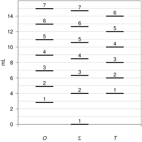
Figure 1: Spectra of states with $mL<15$.

We shall turn now to the scattering amplitudes, which, in an equivalent fashion, describe the decay of a glueball into two other glueballs, or the creation of that glueball in a two-glueball collision. These processes are constrained by phase space such that the mass of the decaying (or the created) glueball must be at least as large as the sum of the masses of the decay products (or the colliding particles). It will turn out that the amplitudes for most processes, which are allowed by phase space, vanish.

In order to simplify the discussion, we have chosen to consider the unpolarized amplitudes for processes involving the spin-two glueballs $T_{k}$. This is achieved by first projecting the generic amplitude containing indices $i$ and $j$ for each external spin-two state onto a particular polarization using the polarization matrices $\varepsilon_{r}(p)^{i}_{j}$, then taking the square and finally summing over all polarizations $r$. For the amplitudes of $T\mathcal{O}\mathcal{O}$ processes this implies

$$|\mathcal{M}_{TOO}|^{2} =\sum\limits_{r=1}^{5}\left[\varepsilon_{r}(p_{1})^{i}_{j}\mathcal{M}_{TOO}{}^{j}_{i}\right]\left[\varepsilon_{r}(p_{1})^{k}_{l}\mathcal{M}_{TOO}{}^{l}_{k}\right]$$

$$=\mathcal{M}_{TOO}{}^{j}_{i}\Pi_{1}{}^{ik}_{jl}\mathcal{M}_{TOO}{}^{l}_{k}~{},$$ (128)

where we have used the completeness relation (126). As $\mathcal{M}_{TOO}{}^{i}_{j}$ is of the form

$$\mathcal{M}_{TOO}{}^{i}_{j}=\left(\Pi_{1}{}^{ik}_{jl}p_{2k}p_{3}^{l}\right)\tilde{\mathcal{M}}_{TOO}~{},$$

we find from (128)

$$|\mathcal{M}_{TOO}|^{2} =\left(p_{2i}p_{2k}p_{3}^{j}p_{3}^{l}\Pi_{1}{}^{ik}_{jl}\right)|\tilde{\mathcal{M}}_{TOO}|^{2}$$

$$=\frac{1}{24p_{1}^{4}}\left(p_{1}^{4}+p_{2}^{4}+p_{3}^{4}-2p_{1}^{2}p_{2}^{2}-2p_{1}^{2}p_{3}^{2}-2p_{2}^{2}p_{3}^{2}\right)^{2}|\tilde{\mathcal{M}}_{TOO}|^{2}~{}.$$ (129)

The last line is easily established in the rest frame of the $T$ particle. The unpolarized amplitude $|\mathcal{M}_{T\Sigma\Sigma}|^{2}$ is obtained in the same fashion.

Similarly, we might define the unpolarized amplitudes $|\mathcal{M}_{OTT}|^{2}$ and $|\mathcal{M}_{TTT}|^{2}$, which give rise to more cumbersome pre-factors involving the external momenta. We shall not provide their explicit expressions, because our numerical analysis will indicate that the amplitudes of all processes of these kinds, which are allowed by phase space, vanish. Hence, the overall factor is of no importance.

The actual calculation of the scattering amplitudes (107) can be easily implemented on a computer. The numerical results for the unpolarized glueball decay amplitudes for the glueball states with $k\leq 10$ are listed in appendix B. Here, we summarize our findings and the resulting decay channels.

The states $\mathcal{O}_{1}$ and $\Sigma_{1}$ turn out to be stable glueballs. For $\Sigma_{1}$ this is natural, because it is massless, but for $\mathcal{O}_{1}$ it results from the fact that the only allowed process, $\mathcal{O}_{1}\to\Sigma_{1}+\Sigma_{1}$, has a zero amplitude. In contrast, the process $T_{1}\to\Sigma_{1}+\Sigma_{1}$ is allowed and occurs.

A glueball $\mathcal{O}_{k}$ with $k>1$ decays mainly into two $\Sigma$ glueballs. It can decay into $\Sigma_{k}+\Sigma_{1}$, and into $\Sigma_{i}+\Sigma_{j}$ such that $i+j=k$, but the latter processes are severely restricted by phase space. In fact, for $k\geq 10$, only the processes $\mathcal{O}_{k}\to\Sigma_{k-2}+\Sigma_{2}$ and $\mathcal{O}_{k}\to\Sigma_{k-1}+\Sigma_{1}$ are allowed. Furthermore, $\mathcal{O}_{k}$ can decay into $\mathcal{O}_{i}+T_{j}$ such that $i+j=k-1$, although these decay channels are much less probable. All other allowed processes have zero amplitudes. In particular, there are no decays of the form $\mathcal{O}\to T+T$ and $\mathcal{O}\to\mathcal{O}+\mathcal{O}$.

The decay of a glueball $\Sigma_{k}$ with $k>1$ must contain exactly one $\Sigma$ glueball amongst the products. The main decay channels are into $\Sigma_{i}+T_{j}$ such that $i+j=k-1$, and into $\mathcal{O}_{k-1}+\Sigma_{1}$. The decay into $T_{k-1}+\Sigma_{1}$ also occurs, but has a much smaller probability. Again, all other allowed processes have vanishing amplitude.

Finally, the glueballs $T_{k}$ decay mainly into two $\Sigma$ glueballs, the main channels being into $\Sigma_{i}+\Sigma_{j}$ such that $i+j=k$, and into $\Sigma_{k}+\Sigma_{1}$. Decays into $\mathcal{O}_{i}+\mathcal{O}_{j}$ such that $i+j=k$ are also possible, but less probable. As before, all other allowed decay processes have vanishing amplitude.

Although our conclusions about the vanishing amplitudes of many decay channels stem from the numerical analysis of the decay amplitudes up to $k=20$, we believe that there is a deeper reason, which is to be sought in some orthogonality relation of the Jacobi polynomials. We shall not try to give a more rigorous proof of these statements.

A comparison of our results with similar data from lattice simulations of $\mathcal{N}=1$ SYM theory, when they become available, would be very interesting.

The three-point function $\left\langle\mathcal{O}\Sigma\Sigma\right\rangle$ has been calculated also by Bianchi and Marchetti [7]. Although their formula differs from our (111), it is possible to show, using integrations by parts and the equations of motion for the bulk-to-boundary propagators, that the two bulk integrals differ only by boundary terms. In the three-point function, these boundary terms would constitute contact terms, which we should drop, because none of us has done a reliable analysis of the contact terms. In the amplitudes, the boundary terms vanish because of factors of $u$ and $(1-u)$. In fact, our numerical amplitudes agree completetly.

In conclusion, the holographic analysis of the three-point functions for the operators $\mathcal{O}$, $\Sigma$ and $T^{i}_{j}$ has yielded precise predictions for the glueball scattering amplitudes in the GPPZ flow. As the GPPZ flow shares some features with pure $\mathcal{N}=1$ SYM theory (in particular confinement), it potentially sheds light on the IR dynamics of the latter. However, one should be cautious to draw too quick a conclusion. The GPPZ flow is a particular, unstable, case of a two-parameter family of $\mathcal{N}=1$ holographic RG flow backgrounds describing the mass deformation of $\mathcal{N}=4$ SYM theory [4]. In a generic member of this family both scalars considered in this paper, $\phi$ and $\sigma$, are active, and the latter describes a gaugino condensate, which is a necessary ingredient in the vacuum structure of $\mathcal{N}=1$ SYM theory. However, all of these backgrounds are singluar, and it is unclear how to choose amongst the parameters the right values that describe an $\mathcal{N}=1$ vacuum. By analogy with other gravity duals of $\mathcal{N}=1$ SYM theory (e.g., the Maldacena-Nuñez solution [23]), one might argue that a truely 10-dimensional mechanism—unknown at present—will resolve the bulk singularities, thereby fixing the parameters and isolating the vacuum.

Hence, one should regard the GPPZ flow as a toy model, whose qualitative features exist also in the theory with the true vacuum. These features include the existence of glueball states and the preferred glueball decay channels, although the numerics of the glueball masses and scattering amplitudes will be affected by the non-zero gluino condensate and the singularity resolution. It might, of course, have been better to consider a generic background of the two-parameter family of solutions in order to describe at least the effect of the gluino condensate. Unfortunately, there are two technical difficulties already at the linearized level making this problem much harder to tackle. First, the two active scalars present in these backgrounds couple to each other through the potential leading to a fourth order differential equation. Second, although the traceless transversal components of the metric decouple from all other fields, their equation of motion is not analytically solvable. Further progress on these issues is, therefore, very desirable.

Appendix A Useful Relations for the GPPZ Flow

We summarize here a number of relations for the GPPZ background. For simplicity, we set the asymptotically AdS length scale to unity, i.e., $L=1$.

The potential $V(\phi,\sigma)$ that gives rise to the GPPZ flow with $\phi$ as an active scalar was found in [4]. It is given in terms of a superpotential $W(\phi,\sigma)$ by

$$V(\phi,\sigma)=\frac{1}{2}\left(\frac{\partial W}{\partial\phi}\right)^{2}+\frac{1}{2}\left(\frac{\partial W}{\partial\sigma}\right)^{2}-\frac{4}{3}W^{2}~{},$$ (130)

where

$$W(\phi,\sigma)=-\frac{3}{4}\left[\cosh\left(\frac{2\phi}{\sqrt{3}}\right)+\cosh(2\sigma)\right]~{}.$$ (131)

Hence, we have

$$V(\phi,\sigma)=-\frac{3}{8}\left[\cosh^{2}\left(\frac{2\phi}{\sqrt{3}}\right)+4\cosh\left(\frac{2\phi}{\sqrt{3}}\right)\cosh(2\sigma)-\cosh^{2}(2\sigma)+4\right]~{}.$$ (132)

The GPPZ background solution is

$$\mathrm{e}^{2\bar{\phi}/\sqrt{3}}=\frac{1+\mathrm{e}^{-r}}{1-\mathrm{e}^{-r}}~{},\qquad\bar{\sigma}=0~{},\qquad\mathrm{e}^{2A}=\mathrm{e}^{2r}-1~{}.$$ (133)

From (133) we easily find the background source,

$$\hat{\bar{\phi}}=\sqrt{3}~{}.$$ (134)

For the GPPZ background (for $\bar{\sigma}=0$), there are a number of identities that simplify the calculations with the potentials and its derivatives, namely

$$W_{\phi\phi} =\frac{4}{3}W+1~{},\quad \frac{W_{\phi}^{2}}{W} =\frac{4}{3}W+2~{},\quad V =-W\left(\frac{2}{3}W-1\right)~{},$$ (135)

$$V_{\sigma\sigma} =8W+9~{}, V_{\sigma\sigma\phi} =8W_{\phi}~{}, V_{\sigma\sigma\sigma} =0~{}.$$

Finally, it is useful to introduce the variable

$$u=1-\mathrm{e}^{-2r}~{},$$ (136)

in terms of which the following relations hold,

$$\frac{du}{dr} =2(1-u)~{},\quad \mathrm{e}^{-2A} =\frac{1-u}{u}~{},$$ (137)

$$W =-\frac{3}{2u}~{}, W_{\phi} =-\sqrt{3}\frac{\sqrt{1-u}}{u}~{}.$$

Appendix B Numerical Results for the Glueball Decay Amplitudes

In this appendix we provide lists of all non-zero scattering amplitudes ($|\mathcal{M}|^{2}$) for the decays of the glueballs $\mathcal{O}_{k}$, $\Sigma_{k}$ and $T_{k}$ with $k\leq 10$. Only the amplitudes for decay processes allowed by the phase space are given. The amplitudes involving $T$ glueballs are the unpolarized ones as defined in Sec. 5.

				$T_{1}\to\Sigma_{1}+\Sigma_{1}$	$184.32$
$T_{2}\to\Sigma_{1}+\Sigma_{1}$	$103.68$	$T_{2}\to\mathcal{O}_{1}+\mathcal{O}_{1}$	$0.08$	$T_{2}\to\Sigma_{2}+\Sigma_{1}$	$81.633$
$T_{3}\to\Sigma_{2}+\Sigma_{1}$	$105.8$	$T_{3}\to\mathcal{O}_{2}+\mathcal{O}_{1}$	$0.145$	$T_{3}\to\Sigma_{3}+\Sigma_{1}$	$51.429$
$T_{4}\to\Sigma_{3}+\Sigma_{1}$	$102.86$	$T_{4}\to\mathcal{O}_{3}+\mathcal{O}_{1}$	$0.179$	$T_{4}\to\Sigma_{4}+\Sigma_{1}$	$38.099$
$T_{4}\to\Sigma_{2}+\Sigma_{2}$	$117.55$	$T_{4}\to\mathcal{O}_{2}+\mathcal{O}_{2}$	$0.287$
$T_{5}\to\Sigma_{4}+\Sigma_{1}$	$99.967$	$T_{5}\to\mathcal{O}_{4}+\mathcal{O}_{1}$	$0.197$	$T_{5}\to\Sigma_{5}+\Sigma_{1}$	$30.847$
$T_{5}\to\Sigma_{3}+\Sigma_{2}$	$119.01$	$T_{5}\to\mathcal{O}_{3}+\mathcal{O}_{2}$	$0.367$
$T_{6}\to\Sigma_{5}+\Sigma_{1}$	$97.601$	$T_{6}\to\mathcal{O}_{5}+\mathcal{O}_{1}$	$0.209$	$T_{6}\to\Sigma_{6}+\Sigma_{1}$	$26.368$
$T_{6}\to\Sigma_{4}+\Sigma_{2}$	$118.3$	$T_{6}\to\mathcal{O}_{4}+\mathcal{O}_{2}$	$0.415$
$T_{6}\to\Sigma_{3}+\Sigma_{3}$	$123.23$	$T_{6}\to\mathcal{O}_{3}+\mathcal{O}_{3}$	$0.481$
$T_{7}\to\Sigma_{6}+\Sigma_{1}$	$95.705$	$T_{7}\to\mathcal{O}_{6}+\mathcal{O}_{1}$	$0.217$	$T_{7}\to\Sigma_{7}+\Sigma_{1}$	$23.356$
$T_{7}\to\Sigma_{5}+\Sigma_{2}$	$117.12$	$T_{7}\to\mathcal{O}_{5}+\mathcal{O}_{2}$	$0.446$
$T_{7}\to\Sigma_{4}+\Sigma_{3}$	$124.22$	$T_{7}\to\mathcal{O}_{4}+\mathcal{O}_{3}$	$0.552$
$T_{8}\to\Sigma_{7}+\Sigma_{1}$	$94.173$	$T_{8}\to\mathcal{O}_{7}+\mathcal{O}_{1}$	$0.223$	$T_{8}\to\Sigma_{8}+\Sigma_{1}$	$21.206$
$T_{8}\to\Sigma_{6}+\Sigma_{2}$	$115.91$	$T_{8}\to\mathcal{O}_{6}+\mathcal{O}_{2}$	$0.467$
$T_{8}\to\Sigma_{5}+\Sigma_{3}$	$124.11$	$T_{8}\to\mathcal{O}_{5}+\mathcal{O}_{3}$	$0.599$
$T_{8}\to\Sigma_{4}+\Sigma_{4}$	$126.37$	$T_{8}\to\mathcal{O}_{4}+\mathcal{O}_{4}$	$0.639$
$T_{9}\to\Sigma_{8}+\Sigma_{1}$	$92.918$	$T_{9}\to\mathcal{O}_{8}+\mathcal{O}_{1}$	$0.227$	$T_{9}\to\Sigma_{9}+\Sigma_{1}$	$19.6$
$T_{9}\to\Sigma_{7}+\Sigma_{2}$	$114.78$	$T_{9}\to\mathcal{O}_{7}+\mathcal{O}_{2}$	$0.482$
$T_{9}\to\Sigma_{6}+\Sigma_{3}$	$123.61$	$T_{9}\to\mathcal{O}_{6}+\mathcal{O}_{3}$	$0.631$
$T_{9}\to\Sigma_{5}+\Sigma_{4}$	$127.07$	$T_{9}\to\mathcal{O}_{5}+\mathcal{O}_{4}$	$0.697$
$T_{10}\to\Sigma_{9}+\Sigma_{1}$	$91.875$	$T_{10}\to\mathcal{O}_{9}+\mathcal{O}_{1}$	$0.23$	$T_{10}\to\Sigma_{10}+\Sigma_{1}$	$18.358$
$T_{10}\to\Sigma_{8}+\Sigma_{2}$	$113.78$	$T_{10}\to\mathcal{O}_{8}+\mathcal{O}_{2}$	$0.493$
$T_{10}\to\Sigma_{7}+\Sigma_{3}$	$122.98$	$T_{10}\to\mathcal{O}_{7}+\mathcal{O}_{3}$	$0.654$
$T_{10}\to\Sigma_{6}+\Sigma_{4}$	$127.14$	$T_{10}\to\mathcal{O}_{6}+\mathcal{O}_{4}$	$0.738$
$T_{10}\to\Sigma_{5}+\Sigma_{5}$	$128.37$	$T_{10}\to\mathcal{O}_{5}+\mathcal{O}_{5}$	$0.764$

Table 1: The unpolarized decay amplitudes for the glueballs $T_{k}$ with $k\leq 10$.

				$\mathcal{O}_{2}\to\Sigma_{2}+\Sigma_{1}$	$64.0$
$\mathcal{O}_{3}\to\Sigma_{2}+\Sigma_{1}$	$3.6571$	$\mathcal{O}_{3}\to\mathcal{O}_{1}+T_{1}$	$0.163$	$\mathcal{O}_{3}\to\Sigma_{3}+\Sigma_{1}$	$100.0$
$\mathcal{O}_{4}\to\Sigma_{3}+\Sigma_{1}$	$8.5714$	$\mathcal{O}_{4}\to\mathcal{O}_{1}+T_{2}$	$0.213$	$\mathcal{O}_{4}\to\Sigma_{4}+\Sigma_{1}$	$116.64$
$\mathcal{O}_{4}\to\Sigma_{2}+\Sigma_{2}$	$39.184$	$\mathcal{O}_{4}\to\mathcal{O}_{2}+T_{1}$	$0.302$
$\mathcal{O}_{5}\to\Sigma_{4}+\Sigma_{1}$	$12.567$	$\mathcal{O}_{5}\to\mathcal{O}_{1}+T_{3}$	$0.233$	$\mathcal{O}_{5}\to\Sigma_{5}+\Sigma_{1}$	$125.44$
$\mathcal{O}_{5}\to\Sigma_{3}+\Sigma_{2}$	$81.455$	$\mathcal{O}_{5}\to\mathcal{O}_{2}+T_{2}$	$0.422$
		$\mathcal{O}_{5}\to\mathcal{O}_{3}+T_{1}$	$0.374$
$\mathcal{O}_{6}\to\Sigma_{5}+\Sigma_{1}$	$15.664$	$\mathcal{O}_{6}\to\mathcal{O}_{1}+T_{4}$	$0.242$	$\mathcal{O}_{6}\to\Sigma_{6}+\Sigma_{1}$	$130.61$
$\mathcal{O}_{6}\to\Sigma_{4}+\Sigma_{2}$	$118.67$	$\mathcal{O}_{6}\to\mathcal{O}_{2}+T_{3}$	$0.479$
$\mathcal{O}_{6}\to\Sigma_{3}+\Sigma_{3}$	$178.0$	$\mathcal{O}_{6}\to\mathcal{O}_{3}+T_{2}$	$0.541$
		$\mathcal{O}_{6}\to\mathcal{O}_{4}+T_{1}$	$0.413$
$\mathcal{O}_{7}\to\Sigma_{6}+\Sigma_{1}$	$18.085$	$\mathcal{O}_{7}\to\mathcal{O}_{1}+T_{5}$	$0.247$	$\mathcal{O}_{7}\to\Sigma_{7}+\Sigma_{1}$	$133.9$
$\mathcal{O}_{7}\to\Sigma_{5}+\Sigma_{2}$	$149.61$	$\mathcal{O}_{7}\to\mathcal{O}_{2}+T_{4}$	$0.509$
$\mathcal{O}_{7}\to\Sigma_{4}+\Sigma_{3}$	$271.35$	$\mathcal{O}_{7}\to\mathcal{O}_{3}+T_{3}$	$0.626$
		$\mathcal{O}_{7}\to\mathcal{O}_{4}+T_{2}$	$0.61$
		$\mathcal{O}_{7}\to\mathcal{O}_{5}+T_{1}$	$0.437$
$\mathcal{O}_{8}\to\Sigma_{7}+\Sigma_{1}$	$20.012$	$\mathcal{O}_{8}\to\mathcal{O}_{1}+T_{6}$	$0.25$	$\mathcal{O}_{8}\to\Sigma_{8}+\Sigma_{1}$	$136.11$
$\mathcal{O}_{8}\to\Sigma_{6}+\Sigma_{2}$	$175.15$	$\mathcal{O}_{8}\to\mathcal{O}_{2}+T_{5}$	$0.526$
$\mathcal{O}_{8}\to\Sigma_{5}+\Sigma_{3}$	$354.58$	$\mathcal{O}_{8}\to\mathcal{O}_{3}+T_{4}$	$0.674$
$\mathcal{O}_{8}\to\Sigma_{4}+\Sigma_{4}$	$429.65$	$\mathcal{O}_{8}\to\mathcal{O}_{4}+T_{3}$	$0.716$
		$\mathcal{O}_{8}\to\mathcal{O}_{5}+T_{2}$	$0.654$
		$\mathcal{O}_{8}\to\mathcal{O}_{6}+T_{1}$	$0.452$
$\mathcal{O}_{9}\to\Sigma_{8}+\Sigma_{1}$	$21.576$	$\mathcal{O}_{9}\to\mathcal{O}_{1}+T_{7}$	$0.252$	$\mathcal{O}_{9}\to\Sigma_{9}+\Sigma_{1}$	$137.67$
$\mathcal{O}_{9}\to\Sigma_{7}+\Sigma_{2}$	$196.36$	$\mathcal{O}_{9}\to\mathcal{O}_{2}+T_{6}$	$0.537$
$\mathcal{O}_{9}\to\Sigma_{6}+\Sigma_{3}$	$427.02$	$\mathcal{O}_{9}\to\mathcal{O}_{3}+T_{5}$	$0.704$
		$\mathcal{O}_{9}\to\mathcal{O}_{4}+T_{4}$	$0.779$
		$\mathcal{O}_{9}\to\mathcal{O}_{5}+T_{3}$	$0.774$
		$\mathcal{O}_{9}\to\mathcal{O}_{6}+T_{2}$	$0.683$
		$\mathcal{O}_{9}\to\mathcal{O}_{7}+T_{1}$	$0.463$
$\mathcal{O}_{10}\to\Sigma_{9}+\Sigma_{1}$	$22.867$	$\mathcal{O}_{10}\to\mathcal{O}_{1}+T_{8}$	$0.253$	$\mathcal{O}_{10}\to\Sigma_{10}+\Sigma_{1}$	$138.81$
$\mathcal{O}_{10}\to\Sigma_{8}+\Sigma_{2}$	$214.15$	$\mathcal{O}_{10}\to\mathcal{O}_{2}+T_{7}$	$0.544$
		$\mathcal{O}_{10}\to\mathcal{O}_{3}+T_{6}$	$0.723$
		$\mathcal{O}_{10}\to\mathcal{O}_{4}+T_{5}$	$0.818$
		$\mathcal{O}_{10}\to\mathcal{O}_{5}+T_{4}$	$0.847$
		$\mathcal{O}_{10}\to\mathcal{O}_{6}+T_{3}$	$0.814$
		$\mathcal{O}_{10}\to\mathcal{O}_{7}+T_{2}$	$0.703$
		$\mathcal{O}_{10}\to\mathcal{O}_{8}+T_{1}$	$0.47$

Table 2: The unpolarized decay amplitudes for the glueballs $\mathcal{O}_{k}$ with $k\leq 10$.

		$\Sigma_{2}\to T_{1}+\Sigma_{1}$	$0.0$	$\Sigma_{2}\to\mathcal{O}_{1}+\Sigma_{1}$	$115.2$
$\Sigma_{3}\to T_{1}+\Sigma_{1}$	$29.623$	$\Sigma_{3}\to T_{2}+\Sigma_{1}$	$0.091$	$\Sigma_{3}\to\mathcal{O}_{2}+\Sigma_{1}$	$91.428$
$\Sigma_{4}\to T_{1}+\Sigma_{2}$	$35.265$	$\Sigma_{4}\to T_{3}+\Sigma_{1}$	$0.49$	$\Sigma_{4}\to\mathcal{O}_{3}+\Sigma_{1}$	$77.143$
$\Sigma_{4}\to T_{2}+\Sigma_{1}$	$44.082$
$\Sigma_{5}\to T_{1}+\Sigma_{3}$	$37.403$	$\Sigma_{5}\to T_{4}+\Sigma_{1}$	$1.0473$	$\Sigma_{5}\to\mathcal{O}_{4}+\Sigma_{1}$	$68.422$
$\Sigma_{5}\to T_{2}+\Sigma_{2}$	$53.432$
$\Sigma_{5}\to T_{3}+\Sigma_{1}$	$52.364$
$\Sigma_{6}\to T_{1}+\Sigma_{4}$	$38.449$	$\Sigma_{6}\to T_{5}+\Sigma_{1}$	$1.6275$	$\Sigma_{6}\to\mathcal{O}_{5}+\Sigma_{1}$	$62.657$
$\Sigma_{6}\to T_{2}+\Sigma_{3}$	$57.215$
$\Sigma_{6}\to T_{3}+\Sigma_{2}$	$64.081$
$\Sigma_{6}\to T_{4}+\Sigma_{1}$	$57.673$
$\Sigma_{7}\to T_{1}+\Sigma_{5}$	$39.04$	$\Sigma_{7}\to T_{6}+\Sigma_{1}$	$2.1737$	$\Sigma_{7}\to\mathcal{O}_{6}+\Sigma_{1}$	$58.595$
$\Sigma_{7}\to T_{2}+\Sigma_{4}$	$59.152$
$\Sigma_{7}\to T_{3}+\Sigma_{3}$	$69.011$
$\Sigma_{7}\to T_{4}+\Sigma_{2}$	$70.982$
$\Sigma_{7}\to T_{5}+\Sigma_{1}$	$61.349$
$\Sigma_{8}\to T_{1}+\Sigma_{6}$	$39.408$	$\Sigma_{8}\to T_{7}+\Sigma_{1}$	$2.6682$	$\Sigma_{8}\to\mathcal{O}_{7}+\Sigma_{1}$	$55.588$
$\Sigma_{8}\to T_{2}+\Sigma_{5}$	$60.283$
$\Sigma_{8}\to T_{3}+\Sigma_{4}$	$71.609$
$\Sigma_{8}\to T_{4}+\Sigma_{3}$	$76.724$
$\Sigma_{8}\to T_{5}+\Sigma_{2}$	$75.784$
$\Sigma_{8}\to T_{6}+\Sigma_{1}$	$64.038$
$\Sigma_{9}\to T_{1}+\Sigma_{7}$	$39.652$	$\Sigma_{9}\to T_{8}+\Sigma_{1}$	$3.1094$	$\Sigma_{9}\to\mathcal{O}_{8}+\Sigma_{1}$	$53.278$
$\Sigma_{9}\to T_{2}+\Sigma_{6}$	$61.003$
$\Sigma_{9}\to T_{3}+\Sigma_{5}$	$73.161$
$\Sigma_{9}\to T_{4}+\Sigma_{4}$	$79.812$
$\Sigma_{9}\to T_{5}+\Sigma_{3}$	$82.119$
$\Sigma_{9}\to T_{6}+\Sigma_{2}$	$79.303$
$\Sigma_{9}\to T_{7}+\Sigma_{1}$	$66.086$
$\Sigma_{10}\to T_{1}+\Sigma_{8}$	$39.822$	$\Sigma_{10}\to T_{9}+\Sigma_{1}$	$3.5011$	$\Sigma_{10}\to\mathcal{O}_{9}+\Sigma_{1}$	$51.45$
$\Sigma_{10}\to T_{2}+\Sigma_{7}$	$61.49$
$\Sigma_{10}\to T_{3}+\Sigma_{6}$	$74.167$
$\Sigma_{10}\to T_{4}+\Sigma_{5}$	$81.687$
$\Sigma_{10}\to T_{5}+\Sigma_{4}$	$85.577$
$\Sigma_{10}\to T_{6}+\Sigma_{3}$	$86.086$
$\Sigma_{10}\to T_{7}+\Sigma_{2}$	$81.987$
$\Sigma_{10}\to T_{8}+\Sigma_{1}$	$67.698$

Table 3: The unpolarized decay amplitudes for the glueballs $\Sigma_{k}$ with $k\leq 10$.

References

• [1] S. S. Gubser, I. R. Klebanov, and A. M. Polyakov, Gauge theory correlators from non-critical string theory, Phys. Lett. B428 (1998) 105–114, [hep-th/9802109].
• [2] E. Witten, Anti-de Sitter space and holography, Adv. Theor. Math. Phys. 2 (1998) 253–291, [hep-th/9802150].
• [3] J. M. Maldacena, The large N limit of superconformal field theories and supergravity, Adv. Theor. Math. Phys. 2 (1998) 231–252, [hep-th/9711200].
• [4] L. Girardello, M. Petrini, M. Porrati, and A. Zaffaroni, The supergravity dual of N = 1 super Yang-Mills theory, Nucl. Phys. B569 (2000) 451–469, [hep-th/9909047].
• [5] R. Apreda, D. E. Crooks, N. Evans, and M. Petrini, Confinement, glueballs and strings from deformed AdS, hep-th/0308006.
• [6] M. Bianchi, O. DeWolfe, D. Z. Freedman, and K. Pilch, Anatomy of two holographic renormalization group flows, JHEP 01 (2001) 021, [hep-th/0009156].
• [7] M. Bianchi and A. Marchetti, Holographic three-point functions: One step beyond the tradition, hep-th/0302019.
• [8] M. Bianchi, M. Prisco, and W. Mück, New results on holographic three-point functions, JHEP 11 (2003) 052, [hep-th/0310129].
• [9] H. Boschi-Filho and N. R. F. Braga, AdS/CFT correspondence and string / gauge duality, hep-th/0312231.
• [10] M. Bianchi, D. Z. Freedman, and K. Skenderis, Holographic renormalization, Nucl. Phys. B631 (2002) 159–194, [hep-th/0112119].
• [11] D. Anselmi, Inequalities for trace anomalies, length of the RG flow, distance between the fixed points and irreversibility, hep-th/0210124.
• [12] S. de Haro, S. N. Solodukhin, and K. Skenderis, Holographic reconstruction of spacetime and renormalization in the AdS/CFT correspondence, Commun. Math. Phys. 217 (2001) 595–622, [hep-th/0002230].
• [13] D. Martelli and W. Mück, Holographic renormalization and Ward identities with the Hamilton-Jacobi method, Nucl. Phys. B654 (2003) 248–276, [hep-th/0205061].
• [14] D. Z. Freedman, S. S. Gubser, K. Pilch, and N. P. Warner, Renormalization group flows from holography supersymmetry and a c-theorem, Adv. Theor. Math. Phys. 3 (1999) 363–417, [hep-th/9904017].
• [15] K. Skenderis and P. K. Townsend, Gravitational stability and renormalization-group flow, Phys. Lett. B468 (1999) 46–51, [hep-th/9909070].
• [16] O. DeWolfe, D. Z. Freedman, S. S. Gubser, and A. Karch, Modeling the fifth dimension with scalars and gravity, Phys. Rev. D62 (2000) 046008, [hep-th/9909134].
• [17] P. Breitenlohner and D. Z. Freedman, Stability in gauged extended supergravity, Ann. Phys. 144 (1982) 249.
• [18] I. R. Klebanov and E. Witten, AdS/CFT correspondence and symmetry breaking, Nucl. Phys. B556 (1999) 89–114, [hep-th/9905104].
• [19] W. Mück and K. S. Viswanathan, Regular and irregular boundary conditions in the AdS/CFT correspondence, Phys. Rev. D60 (1999) 081901, [hep-th/9906155].
• [20] M. Abramowitz and I. A. Stegun, eds., Handbook of Mathematical Functions. Dower Publ., New York, 1965.
• [21] I. S. Gradshteyn and I. M. Ryzhik, Table of Integrals, Series and Products. Academic Press, New York, 5 ed., 1994.
• [22] M. E. Peskin and D. V. Schroeder, An Introduction to Quantum Field Theory. Perseus Books, Cambridge, Massachusetts, 1995.
• [23] J. M. Maldacena and C. Nunez, Towards the large n limit of pure n = 1 super yang mills, Phys. Rev. Lett. 86 (2001) 588–591, [hep-th/0008001].