Extracting Data from Behind Horizons with the AdS/CFT Correspondence

Recent work has shown that boundary correlators in AdS-Schwarzschild can probe the geometry near the singularity. In this paper we aim to analyze the specific signatures of the singularity, show how significant they can be, and uncover the origins of these large effects in explicitly outside the horizon descriptions.

We add perturbations to the metric localized near the singularity and explore their effects on the boundary correlators. Then we use analyticity arguments to show how this information arises from the Euclidean path integral of a free scalar field in the bulk.

Introduction

In physics we are often able to understand a new object by probing it with something we are already familiar with. This standard approach fails when applied to spacelike singularities because our probes cannot get close to spacelike singularities and live to tell about them - they become trapped behind horizons longs before they approach the singularity itself. However, the structure of a singularity can be probed by spacelike geodesics, and in the AdS/CFT correspondence such geodesics approximate opposite sided boundary correlators. These ideas helped motivate previous work [1], [3], [4], and [5] where it was shown that information about the singularity could be extracted from these correlation functions. Our purpose here is to show that these correlators really do contain information about the geometry near the singularity, and to give explicit examples demonstrating that it is ‘easy’ to access this data. Most of these examples utilize the geodesic approximation.

In [4] it was shown that there exists a dual description of physics in $D=3$ AdS-Schwarzschild, depending on whether one analytically continues the Euclidean metric with respect to Schwarzschild or Kruskal time. In the Schwarzschild description, all quantities can be determined with outside the horizon calculations. Since we are extracting information about the neighborhood of the singularity, it is surprising that we can see large effects from outside the horizon computations. Thus our final calculation will be an attempt to show how the large effects arise from the full quantum path-integral. The key will be analyticity.

The layout of the paper is as follows. After a short review of the AdS-Schwarzschild spacetimes, we use the WKB approximation to explore the effects of a simple perturbation localized near the black hole singularity in the $D=3$ case. This is simply a small change in the geometry near the singularity; it is not required to satisfy Einstein’s equation and we do not expect it to be a model for anything physical. Its purpose is to illustrate that we can explore the geometry with boundary correlators by studying them as a function of the boundary time. We find that the perturbation produces a significant change in the correlators for relatively small values of the boundary time, indicating that information from behind the horizon is not difficult to extract, at least for a meta-observer who can compute any gauge theory amplitude. Moving on to a $D=5$ example, we make a very naive ‘stringy perturbation’ to the metric that resolves the singularity, and investigate the consequences (this is not intended as a guess at what string theory does, it is just a possibility). We find that a pole in the opposite sided correlators resulting from geodesics that ‘bounce’ off the singularity in the unperturbed case splits into two poles above and below the real axis. This is a distinct, unambiguous signature that we have removed the singularity.

Previous work has focused on the idea of behind the horizon data made available from amplitudes computed outside the horizon, far from the black hole. Thus as a concrete example, we calculate approximately how many terms in a power series of the opposite sided correlator as a function of boundary time one must compute in order to see a large change resulting from a small perturbation at the singularity. We find that for a perturbation decaying as $e^{-ar}$ it is only necessary to calculate $O(a)$ terms. Finally, we set up the full quantum calculation of correlation functions for a free scalar field in a perturbed Euclidean $D=3$ background. We expand to first order in the perturbation and derive a geodesic approximation, showing that in the Euclidean case the quantum computation is consistent with the WKB approximation. This shows by virtue of the analyticity of multi-point functions that the large effects of the perturbation must be reproduced in path integral computations.

Spacetime Geometry

Here we will be considering the effects of perturbations to the $D=3$ and $D=5$ AdS-Schwarzschild geometry localized near the black hole singularity. In both cases the metric takes the form

$$ds^{2}=-f(r)dt^{2}+\frac{dr^{2}}{f(r)}+r^{2}d\Omega^{2}$$ (1)

Henceforth, we will ignore spherical part. The function

$$f(r)=r^{2}-1-g(r)$$ (2)

for the $D=3$ case and

$$f(r)=r^{2}-\frac{1}{r^{2}}-g(r)$$ (3)

for the $D=5$ case, with $g(r)$ a ‘small’ perturbation function for both cases. It is essential that we always choose an analytic $g(r)$ function to maintain equivalence with the boundary gauge theory, whose correlation functions are analytic. In these backgrounds the geodesic equations take the form

$$\left(\frac{dr}{ds}\right)^{2} = E^{2}+f(r)$$ (4)

$$\frac{dt}{ds}f(r) = E$$ (5)

The WKB approximation to the opposite-sided boundary two-point function is given by $e^{-mL}$, where $L$ is the proper length of the geodesic connecting the two points. Thus these geodesic equations will be used extensively, beginning in the next section.

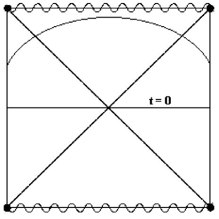
Figure 1: This figure shows the Penrose diagram for the $D=3$ AdS-Schwarzschild spacetime with a symmetric spacelike geodesic passing near the singularity. The $D=5$ case has a similar diagram, with one important difference - the singularities must ‘bend outward’, as shown in [5].

Some $D=3$ Examples

Geodesics Far From the Singularity

First we will give a very simple argument showing in general that the effect of any $g(r)$ perturbation is appropriately small for geodesics far from the singularity. Integrating equation (4) we find

$$L=\lim_{R_{c}\to\infty}\left[2\int_{r_{m}}^{R_{c}}\frac{dr}{\sqrt{E^{2}+f(r)}}-2\mathrm{Log}(R_{c})\right]$$ (6)

The factor of 2 comes from the two parts of a symmetric geodesic, the $-$Log$(R_{c})$ is a regulator, and $r_{m}$ is chosen to satisfy $E^{2}+f(r_{m})=0$, so it is interpreted as the minimum of the $r$ coordinate along the geodesic curve. Since the perturbation $g(r)$ is localized near the singularity and decreases away from it, the maximum of $g(r)$ is at $r_{m}$. But $r_{m}$ must itself be quite large (of order 1 with our dimensionless setup) because the geodesic was taken to be far from the singularity, so $g(r_{m})$ must be extremely small. This gives a bound for $L$ (from now on the regulator will be implicit)

$$2\int_{r_{m}}^{\infty}\frac{dr}{\sqrt{E^{2}+r^{2}-1-|g(r_{m})|}}\leq L\leq 2\int_{r_{m}}^{\infty}\frac{dr}{\sqrt{E^{2}+r^{2}-1+|g(r_{m})|}}$$ (7)

which gives

$$\mathrm{Log}\left(\frac{4}{-E^{2}+1+|g(r_{m})|}\right)\leq L\leq\mathrm{Log}\left(\frac{4}{-E^{2}+1-|g(r_{m})|}\right)$$ (8)

from which we see that $L$ doesn’t change much for geodesics far from the singularity, because such geodesics are characterized by small $E$, and in that range there is no sensitivity to the tiny $|g(r_{m})|$ terms. In other words, the change in $L$ is $\sim|g(r_{m})|$.

Exponential Decay Models

Now we will study a perturbation that decays exponentially as a function of the $r$ coordinate. More precisely, we take $g(r)=\lambda^{2}e^{-ar}$, where we will be taking $a\gg 1$. In this case, even at the black hole horizon, where $r=1$, the perturbation will be exponentially small.

We are interested in correlation functions. In the large mass limit, we can use the WKB approximation, which is based on our knowledge of

$$L=2\int_{r_{m}}^{\infty}\frac{dr}{\sqrt{E^{2}+r^{2}-1-\lambda^{2}e^{-ar}}}$$ (9)

There is no hope of doing this integral explicitly. It can be accurately approximated if it is split into two integrals, but this would involve us in complex algebra that can be avoided by a more direct approach. First note that in the standard, unperturbed case, as the geodesic approaches the singularity, we have

$$L=2\int_{r_{m}}^{\infty}\frac{dr}{\sqrt{r^{2}-r_{m}^{2}}}\to 2\log(r_{m})$$ (10)

as $r_{m}\to 0$. The exact solution in this case [4] gives $L\approx t$ as $t\to\infty$, which is what we are seeing in the equation above. However, with the perturbation turned on, we get an integrand of the form $(Ar^{2}+Br+C)^{-\frac{1}{2}}$ from the expansion of the exponential at very small $r$, so both $L$ and $t$ are finite as $r_{m}\to 0$.

It is possible that we can recover a behavior similar to the unperturbed case by continuing $r_{m}$ past $0$, and in fact, this is exactly what happens. The idea is this: we want to find an $r_{m}$ that takes the integrals for $L$ and $t$ to $\infty$. Near this $r_{m}$ the integrand must behave like $\frac{dx}{\sqrt{x^{2}}}$. Thus we need to find a quadratic vanishing point of the function under the square root, namely $E^{2}+r^{2}-1-\lambda^{2}e^{-ar}$. This is easy to do, the result is that in the regime where $a\lambda<\sqrt{\frac{2}{e}}$, we definitely have an $r_{m}$ value on the negative real r-axis. This is what we would like, since it simply means the true singularity has ‘moved’. However, outside of this regime we still have an $r_{m}$ that allows for quadratic vanishing under the square root, but it will in general be complex, giving a complex $E$ and generically complex $L$ and $t$. Thus we will still find $L\approx ct$ for some $c$, but the physical interpretation is less clear.

In the regime $a\lambda\ll 1$ we can approximate using

$$0=E^{2}+r_{m}^{2}-1-\lambda^{2}e^{-ar_{m}}\approx A\left(r_{m}+\frac{B}{2A}\right)^{2}+C-\frac{B^{2}}{4A}$$ (11)

by expanding the exponential to quadratic order and completing the square. Now if we set $C=\frac{B^{2}}{4A}$ by tuning $E$ we find that $r_{m}=-\frac{B}{2A}$. This allows us to approximate the quadratic vanishing as

$$L = 2\int_{r_{m}}^{R_{t}}\frac{dr}{\sqrt{A\left(r+\frac{B}{2A}\right)^{2}+C-\frac{B^{2}}{4A}}}$$

$$t = 2\int_{r_{m}}^{R_{t}}\frac{Edr}{(1-r^{2}+\lambda^{2}e^{-ar})\sqrt{A\left(r+\frac{B}{2A}\right)^{2}+C-\frac{B^{2}}{4A}}}$$ (12)

where $R_{t}$ is some small value of $r$ where higher order terms from the exponential become important. Both of these integrals do indeed diverge as we approach the $r_{m}$ noted above, and we can roughly approximate $L\approx\left(1+\frac{3a^{2}\lambda^{4}}{8}\right)t$ for very large $t$ by setting the rest of the integrand equal to its value at $r_{m}$. Thus we get a linear $L(t)$ for large $t$ that is larger than in the unperturbed case.

The next example is $g(r)=\lambda^{2}e^{-ar^{2}}$. We can use a similar approximation scheme, but we will get different results - $L\to\infty$ as $r_{m}\to 0$, so the analysis is simplified. This is because when we expand the exponential we find

$$(1+\lambda^{2}a)r_{m}^{2}+(E^{2}-1-\lambda^{2})=Ar_{m}^{2}+B\approx 0$$ (13)

so the perturbation does not destroy the quadratic vanishing at $r_{m}=0$. Again, it is possible to approximate the integral by breaking it up, but a simpler analysis gives the large $t$ behavior. The important point here is that this behavior comes from the region very close to $r_{m}=0$, so we can ignore the rest of the integral. We find

$$t=2\int_{r_{m}}^{R_{t}}\frac{Edr}{\sqrt{Ar^{2}+B}(r^{2}-1-\lambda^{2}e^{-ar^{2}})} \approx 2\int_{r_{m}}^{R_{t}}\frac{\sqrt{1+\lambda^{2}}dr}{\sqrt{Ar^{2}+B}(1+\lambda^{2}-r^{2}(1+\lambda^{2}a))}$$ (14)

$$\approx \frac{L}{\sqrt{1+\lambda^{2}}}$$

So we see that for very small $r_{m}$ corresponding to very large $t$, $L(t)\approx t\sqrt{1+\lambda^{2}}$, which is again larger than in the unperturbed case.

A final question about the exponential decay models is at what value of $t$ does the perturbed $L(t)$ differ significantly from the original $L(t)$? A quick way to get a rough estimate is to use equation (5) to compare an infinitesimal perturbed geodesic length element, $\delta s$, to an unperturbed length element, $\delta s_{0}$, both at a point $r$:

$$\frac{\delta s}{\delta s_{0}}=\frac{r^{2}-1-g(r)}{r^{2}-1}$$ (15)

Thus for a perturbation $g(r)=\lambda^{2}e^{-ar^{b}}$, this expression is significantly different from unity for $r<a^{-1/b}$. Here we interpret $r$ as $r_{m}$, the $r$ of closest approach, so we see that the presence of $g(r)$ starts to make a difference for $r_{m}^{2}=1-E^{2}\approx a^{-2/b}$. At this level of approximation we can use the unperturbed expression for $t(E)$, giving

$$t_{s}\approx\mathrm{Log}(4a^{\frac{2}{b}}-1)$$ (16)

where $t_{s}$ is the value of $t$ where the perturbed and unperturbed $L(t)$ functions begin to separate. Even for very large $a$ this is quite small, indicating that information about the geometry near the singularity is not difficult to recover from boundary correlators.

We can also approach the problem by estimating $\Delta L$, the difference between the perturbed and unperturbed geodesic length, and comparing it to the exact, unperturbed answer. To do this, note that

$$\Delta L(E)=-2\int_{r_{0}}^{r_{m}}\frac{dr}{\sqrt{E^{2}+r^{2}-1}}+2\int_{r_{m}}^{\infty}\frac{dr}{\sqrt{E^{2}+r^{2}-1-\lambda^{2}e^{-ar^{b}}}}-\frac{dr}{\sqrt{E^{2}+r^{2}-1}}$$ (17)

where $r_{0}$ and $r_{m}$ are zeroes of $E^{2}+f(r)=0$ for the unperturbed and perturbed cases, respectively.

We will bound the second term and then compute the first. A similar result will be important in the $D=5$ case for different purposes. The second term is smaller than

$$2\int_{r_{m}}^{\infty}\frac{dr}{\sqrt{E^{2}+r^{2}-1-\lambda^{2}e^{-ar_{m}^{b}}}}-\frac{dr}{\sqrt{E^{2}+r^{2}-1}}=2\mathrm{Log}\left(1+\frac{\lambda^{2}e^{-ar_{m}^{b}}}{r_{m}}\right)$$ (18)

whereas the first term is just

$$-2\mathrm{Log}\left(\frac{r_{m}+\lambda e^{-ar_{m}^{b}/2}}{r_{0}}\right)$$ (19)

Since they contribute with opposite signs and the absolute value of the first term is bigger, we see that (taking absolute values)

$$2\mathrm{Log}\left(\frac{r_{m}(r_{m}+\lambda e^{-ar_{m}^{b}/2})}{r_{0}(r_{m}+\lambda^{2}e^{-ar_{m}^{b}})}\right)<\Delta L(E)<2\mathrm{Log}\left(\frac{r_{m}+\lambda e^{-ar_{m}^{b}/2}}{r_{0}}\right)$$ (20)

and both bounds are reasonable approximations for $\Delta L$ itself. Now we are interested in $\frac{|\Delta L|}{|L_{0}|}$, or upon simplification

$$\frac{\log\left(\frac{r_{m}+\lambda e^{-ar_{m}^{b}/2}}{r_{0}}\right)}{\log(2r_{0})}$$ (21)

Thus we see that for $r_{m}\sim a^{-\frac{1}{b}}$ and so $t\approx\log(a)$, the perturbed $L$ differs from the unperturbed by a sizable percentage, confirming our simpler method above. It is essential to remember that this method and the previous are only estimates. We have been calculating $L$ as a function of $r_{m}$, not $t$, so we can only get a rough idea of when the perturbation becomes important.

Since both methods give an imprecise, but very encouraging estimate for the $t$ value where the perturbation becomes important, we will also give an upper bound above which the perturbation must affect $L$ significantly. We found the exact asymptotic behavior for $L(t)$, and for both exponential models it was $L\approx ct$ for large $t$, for some $c$, where $c=1$ in the unperturbed case. Once in this asymptotic regime, the perturbation is certainly important. This regime is characterized by an $L$ dominated by the segment of the geodesic close to the singularity. Noting that for $t=0$ we have $r_{m}=1$ and $L=2\log(2)$, we see that if $L\gg 1$, $L$ must be dominated by contributions from inside the horizon. Since $L\varpropto t$, for any $t\gg 1$ the perturbation makes a large effect, so in particular, for $t\approx a$ the perturbation must be significant. Thus our previous analyses show that the perturbation should be important for $t\approx\log(a)$, and this calculation demonstrates that its effect will certainly have been long established for $t\approx a$.

An Exactly Solvable Model

The last perturbation to be considered for $D=3$, $g(r)=\frac{\lambda}{r^{2}}$, is really a very large perturbation near the singularity, but it has the advantage that all integrals can be done exactly. Now we have

$$L=2\int_{r_{m}}^{\infty}\frac{dr}{\sqrt{E^{2}+r^{2}-1-\frac{\lambda}{r^{2}}}}$$ (22)

The integral is doable though nontrivial, defining $r_{m}$ as root of the denominator of the integrand, we get the final result

$$L=\mathrm{Log}\left(\frac{4}{E^{2}-1+2r_{m}^{2}}\right)$$ (23)

Note that as $r_{m}\to 0$, the $\frac{\lambda}{r^{2}}$ term implies that $E\to\infty$, implying that $L\to-\infty$. This is dramatically different from the unperturbed case because of the minus sign, but this is not surprising since the effect is huge near $r=0$. The effect here is actually essentially the same as in the standard $D=5$ model, which is obvious given the similar behavior of this perturbation and the $D=5$ model near the singularity. To see this more concretely, note that

$$t=2\int_{r_{m}}^{\infty}\frac{Edr}{(r^{2}-1-\frac{\lambda}{r^{2}})\sqrt{E^{2}+r^{2}-1-\frac{\lambda}{r^{2}}}}$$ (24)

As noted above, the limit $r_{m}\to 0$ corresponds to $E\to\infty$, so in this limit the $E$ dependent terms in the numerator and denominator of the integrand cancel, and we have

$$t=2\int_{0}^{\infty}\frac{dr}{r^{2}-1-\frac{\lambda}{r^{2}}}$$ (25)

which is finite since there is no divergence from $r$ near $0$ or $\infty$. This gives a $t_{c}$ similar to that found by [5] in the $D=5$ case, where there is a pole in the WKB correlator $e^{-mL}$ and the behavior of the $L(t)$ function changes qualitatively. We can evaluate $t_{c}$ explicitly, simplification gives

$$t_{c}=\frac{2\pi}{\sqrt{2+8\lambda}}\left(\sqrt{1+\sqrt{1+4\lambda}}+\sqrt{\sqrt{1+4\lambda}-1}\right)$$ (26)

Model Stringy Effects in $D=5$

Now we will consider a different sort of perturbation in the $D=5$ case. The goal here is to examine how boundary correlators change in a model where the curvature singularity at $r=0$ is ‘resolved’, so that curvature scalars are large and finite where they used to be singular. This could be considered as a model for stringy effects that smear the singularity, but it is not intended as an actual guess at what these effects are. Thus we will take

$$f(r)=r^{2}-\frac{1}{r^{2}+\epsilon^{2}}$$ (27)

so that the $\epsilon=0$ case corresponds to standard AdS-Schwarzchild. In the standard case there exists a special value $t_{c}=\frac{\pi}{2}$ that corresponds to the geodesic becoming nearly null, so that $L\to-\infty$ and the two point correlator blows up. We will find that this $t_{c}$ value is ‘resolved’ when $\epsilon\neq 0$, so that the pole in the boundary correlator at $t_{c}$ splits into two poles, both off the real $t$ axis.

It will be relevant in the following to note that when $t$ and $L$ are regarded as functions of $E$, the $t_{c}$ point corresponds to $E\to\infty$. The integral representation of $t(E)$ for the finite $\epsilon$ case can be parameterized as

$$t=-\int_{r_{m}^{2}}^{\infty}\frac{Edx\sqrt{x+\epsilon^{2}}}{(x-\frac{1}{x+\epsilon^{2}})\sqrt{x^{3}+(E^{2}+\epsilon^{2})x^{2}+(E^{2}\epsilon^{2}-1)x}}$$ (28)

Note that as $E\to\frac{1}{\epsilon}$, the coefficient of $x$ under the square root in the denominator vanishes. Since in this same limit we have $r_{m}=0$, the integrand blows up as $\frac{1}{x}$, so $t\to\infty$, which never occurs in the unperturbed case. Thus for finite but very small $\epsilon$, $t(E)$ increases steadily for a while, levels off near $t_{c}$, then blows up to infinity for $E$ near $\frac{1}{\epsilon}$. Note that this divergence comes from the behavior of the integrand near $x=0$, but the only difference between this integrand and the integrand for the $L(E)$ function is the factor of $(x-\frac{1}{x+\epsilon^{2}})$ in the denominator and the factor of $E$ in the numerator. These factors combine to give $L(t)\approx\frac{t}{\epsilon}$ for $E$ near $\frac{1}{\epsilon}$, or $t\to\infty$.

However, this leaves us with a mystery, because in the original model $L(t)\approx 2\mathrm{Log}(t-t_{c})$ near $t_{c}$. Where has this $t_{c}$ singularity gone? To answer this question we look at

$$L(E)=\int_{r_{m}^{2}}^{\infty}\frac{dx\sqrt{x+\epsilon^{2}}}{\sqrt{x^{3}+(E^{2}+\epsilon^{2})x^{2}+(E^{2}\epsilon^{2}-1)x}}$$ (29)

because we must have $L(t)\to-\infty$ at the new value(s) of $t_{c}$. For very large $E$ (much greater than $\frac{1}{\epsilon}$) the integral expression for $L$ gets large, because there is a large range of $x$ where the integrand is only decaying like $x^{-1/2}$.

To see this explicitly, we can approximate $L(E)$ very roughly in this regime as

$$L=\int_{-\epsilon^{2}}^{\epsilon^{2}}\frac{\epsilon dx}{\sqrt{E^{2}x^{2}+(E^{2}\epsilon^{2}-1)x}}+\int_{\epsilon^{2}}^{\infty}\frac{dx}{\sqrt{x^{2}+E^{2}x+E^{2}\epsilon^{2}-1}}$$ (30)

(the lower limit of integration is $-\epsilon^{2}$, not $0$, because $-\epsilon^{2}$ is the largest root of $E^{2}+f(r)=0$) which gives

$$L=\frac{2\epsilon}{E}\mathrm{Log}(2i+2iE\epsilon)+\frac{2\epsilon^{2}}{E}\mathrm{Log}(2E\epsilon+2\sqrt{E^{2}\epsilon^{2}-1})-\mathrm{Log}\left(2\epsilon^{2}+E^{2}+2\sqrt{2E^{2}\epsilon^{2}-1}\right)$$ (31)

The first two terms go to $0$ for large $E$, but the third term goes to $-\infty$. This divergence arises from the large $x$ behavior of the integrand, which explains why $t$ is finite for large $E$ - its integrand includes an extra factor of $\frac{1}{x}$. Thus despite the singularity in $t$ at $E=\frac{1}{\epsilon}$, it still makes sense to consider the limit $E\to\infty$ in our search for the missing pole, because for very large $E$, $L$ diverges while $t$ stays finite (close to the original $t_{c}$ but slightly complex), imitating the $t_{c}$ behavior of the unperturbed model. Calculating the full approximate value of $t(E)$ is a bit lengthy, but the imaginary part of $t_{c}$ is easier because it must come from the region where $x$ is negative. Thus we can get it from

$$\mathrm{Im}(t_{c}) \approx \mathrm{Im}\left(\int_{-\epsilon^{2}}^{\epsilon^{2}}\frac{-E\epsilon(x+\epsilon^{2})}{\sqrt{E^{2}x^{2}+(E^{2}\epsilon^{2}-1)x}}\right)$$ (32)

$$= \pm\frac{i\pi\epsilon^{3}}{2}$$

where the $\pm$ comes from the choice of sign in the square roots of negative quantities. This shows how a perturbation that ‘resolves’ the black hole singularity splits the Log$(t-t_{c})$ pole. Without the perturbation we had $L(t)\approx 2\mathrm{Log}(t-t_{c})$ near $t_{c}$, so this must be modified at finite $\epsilon$. A good guess would be that $L(t)\approx\mathrm{Log}((t-t_{c+})(t-t_{c-}))$, but this remains an estimate because the integrals cannot be done algebraically.

Perturbations and Power Series

In this section we study $f(r)=r^{2}-\frac{1+e^{-ar}}{r^{2}}$ in the $D=5$ case. In particular, we will analyze the power series for $L(t)$ and show that the coefficients of this power series differ from the coefficients of the unperturbed case by an amount larger than the original coefficients after only $a$ terms. This suggests that from a computational point of view our calculations are surprisingly sensitive to the geometry near the singularity. Though we choose this model for variety, our methods carry over straightforwardly to the $D=3$ exponential models studied earlier.

First we note that for small $E$, $t(E)\approx E$, so we will only worry about the $L(E)$ function - studying small $E$ is equivalent to studying small $t$. This is an approximation, because we are assuming that higher powers of $t$ in $E(t)$ do not conspire to destroy the results we find. First consider the unperturbed $L(E)$ function

$$L_{0}(E)=2\int_{r_{0}}^{\infty}\frac{dr}{\sqrt{E^{2}+r^{2}-\frac{1}{r^{2}}}}=\mathrm{Log}\left(\frac{1}{\sqrt{1+\frac{E^{4}}{4}}}\right)$$ (33)

where the denominator of the integrand is zero at $r_{0}$. It will be useful later to note that the coefficient of the $4n^{th}$ term in the expansion of $r_{0}(E)$ is given approximately by $\frac{1}{n4^{n}}$. Even more roughly, the coefficient of the $n^{th}$ power of $E$ in the expansion of $L_{0}(E)$ is about $2^{-n/2}$. Now define

$$\Delta L(E)=2\int_{r_{m}}^{\infty}\frac{dr}{\sqrt{E^{2}+r^{2}-\frac{1+e^{-ar}}{r^{2}}}}-2\int_{r_{0}}^{\infty}\frac{dr}{\sqrt{E^{2}+r^{2}-\frac{1}{r^{2}}}}$$ (34)

where $r_{m}$ satisfies $E^{2}+f(r_{m})=0$ in the perturbed case. We will now examine the power series for $r_{m}$; this will be important because later we will show that the coefficients of the power series for $\Delta L(E)$ are essentially proportional to the coefficients in the series for $r_{m}(E)$. We can write

$$r_{m}=1+x+\sum c_{k}E^{k}$$ (35)

which we can plug into the defining equation to get

$$E^{2}(1+x+\sum c_{k}E^{k})^{2}+(1+x+\sum c_{k}E^{k})^{4}-1-e^{-a-ax}e^{a\sum c_{k}E^{k}}=0$$ (36)

We can then use this equation to solve for the $c_{k}$ by equating powers of $E$. Assuming $x$ has been correctly computed the coefficients of all the odd powers of $E$ will vanish (since the equation defining $r_{m}$ only involves $E^{2}$). We compute $c_{2}$ as

$$E^{2}+4(1+3x)c_{2}E^{2}-e^{-a-ax}ac_{2}E^{2}=0$$

$$\Rightarrow c_{2}\approx\frac{1}{4}$$ (37)

Now we only need to keep the $c_{2}$ part when we expand the exponential, because terms involving higher $c_{n}$ will have fewer factors of $a$, which is a large number. By expanding the exponential we find

$$c_{n}\approx\frac{e^{-a}a^{n}}{n!2^{n/2}}\approx\frac{e^{-a}a^{n}}{n^{n}e^{-n}2^{n/2}}$$ (38)

What we are interested in is the ratio of these terms to the terms in the expansion of $L_{0}$. This ratio is $\frac{e^{-a}a^{n}}{n^{n}e^{-n}}$, and it is maximized at the $a^{th}$ term, which is of order $1$.

Now looking back to equation (34) and noting that $r_{m}>r_{0}$, we can write

$$\Delta L(E)=2\int_{r_{0}}^{r_{m}}\frac{-dr}{\sqrt{E^{2}+r^{2}-\frac{1}{r^{2}}}}+2\int_{r_{m}}^{\infty}\frac{dr}{\sqrt{E^{2}+r^{2}-\frac{1+e^{-ar}}{r^{2}}}}-\frac{dr}{\sqrt{E^{2}+r^{2}-\frac{1}{r^{2}}}}$$ (39)

We will now show that the contribution of the second term to the power series is exponentially suppressed as $e^{-a/2}$, and that the first term contributes to the power series of $\Delta L(E)$ terms proportional to (or larger than) the $r_{m}$ series. First we bound the second term. There is no theorem here that says that our bound on the second term also bounds the power series in $E$, but it should be extremely plausible in this case, because our bound does not destroy any violent dependence on $E$. In any case, we can always just regard our bound as an approximation. It is

$$2^{nd}\mathrm{\ term} < 2\int_{r_{m}}^{\infty}\frac{dr}{\sqrt{E^{2}+r^{2}-\frac{1+e^{-ar_{m}}}{r^{2}}}}-\frac{dr}{\sqrt{E^{2}+r^{2}-\frac{1}{r^{2}}}}$$ (40)

$$= \mathrm{Log}\left(1+\frac{e^{-ar_{m}}}{AB}-\frac{e^{-2ar_{m}}}{4AB^{3}}+...\right)$$

where $B=r_{m}e^{-ar_{m}/2}$ and $A=E^{2}+2r_{m}^{2}+2B$. Thus every term is suppressed by $e^{-ar_{m}/2}$, which proves the claim since $r_{m}$ is nearly $1$ for $t$ near $0$. Now we need only show that the first term gives the much larger contribution claimed. This is not very hard, because we can just evaluate the first term directly, it is

$$2\int_{r_{0}}^{r_{m}}\frac{-dr}{\sqrt{E^{2}+r^{2}-\frac{1}{r^{2}}}} = \mathrm{Log}\left(\frac{E^{2}+2r_{m}^{2}+2\sqrt{r_{m}^{4}+E^{2}r_{m}^{2}-1}}{E^{2}+2r_{0}^{2}}\right)$$

$$= \mathrm{Log}\left(1+\frac{2r_{0}^{2}\sqrt{2r_{m}-2r_{0}}}{\sqrt{r_{0}+r_{0}^{5}}}+\frac{4r_{0}^{2}(r_{m}-r_{0})}{1+r_{0}^{4}}+...\right)$$

which when expanded gives a power series in $E$ with terms at least as large as the $r_{m}$ series, because $r_{0}\approx 1$. Thus we have shown that after about $a$ terms the $\Delta L(E)$ power series has coefficients that are large compared to the $L_{0}(E)$ coefficients. This is noteworthy because the perturbation itself is suppressed exponentially in $a$.

Path Integral Treatment

All previous results have been obtained from the WKB approximation, which applies in the large mass limit. Thus it would be interesting to see how large effects emerge from a small perturbation in the full quantum mechanical treatment of the problem. Furthermore, in [4] it was shown that there exists a dual description of the $D=3$ AdS-Schwarzschild physics, depending on whether Lorentzian correlators are obtained from the Euclidean correlator through analytic continuation with respect to the Schwarzschild time coordinate or Kruskal time. Thus it should be possible to see the large effects in an explicitly outside the horizon calculation. We will see how this is done, and the key will be analytic continuation.

We wish to calculate the two point function for a massive free scalar field in the perturbed S-AdS background. Specifically, we want to evaluate this two point function between field operators on opposite sides of the Penrose diagram, with the black hole between them, so that we can compare the effect of the perturbations with the semi-classical treatment already given. In order to do this, we will compute in the Euclidean spacetime, and then analytically continue in the $t$ coordinate. The primary object we will consider is the Euclidean path integral

$$I=\int D\Phi\ e^{-\int\frac{d^{3}x}{2}\left[\frac{(\partial_{t}\Phi)^{2}}{r^{2}-1-g(r)}+(r^{2}-1-g(r))(\partial_{t}\Phi)^{2}+\frac{(\partial_{\phi}\Phi)^{2}}{r^{2}}+m^{2}\Phi^{2}\right]}$$ (42)

Now for $g(r)=\lambda^{2}e^{-ar^{2}}$ we can expand the argument of the exponential to first order in $\lambda^{2}$, to get

$$I\approx\int D\Phi\ e^{-\int\frac{d^{3}x}{2}(\lambda^{2}e^{-ar^{2}})\left[\frac{1}{(r^{2}-1)^{2}}(\partial_{t}\Phi)^{2}+(\partial_{r}\Phi)^{2}\right]}\ e^{-\int\frac{d^{3}x}{2}\left[\frac{(\partial_{t}\Phi)^{2}}{r^{2}-1}+(r^{2}-1)(\partial_{t}\Phi)^{2}+\frac{(\partial_{\phi}\Phi)^{2}}{r^{2}}+m^{2}\Phi^{2}\right]}$$ (43)

Note that the integrals are only evaluated outside the horizon, since the behind the horizon region doesn’t even exist in the euclidean case. Now we have approximated the first order effect of the perturbation as an insertion of an operator smeared over spacetime. Thus the two point function can be written as

$$\langle\Phi(x_{1})\Phi(x_{2})\rangle \approx \left\langle\Phi_{0}(x_{1})\Phi_{0}(x_{2})e^{-\int\frac{d^{3}x}{2}(\lambda^{2}e^{-ar^{2}})\left[\frac{1}{(r^{2}-1)^{2}}(\partial_{t}\Phi_{0})^{2}+(\partial_{r}\Phi_{0})^{2}\right]}\right\rangle$$

$$\approx \left\langle\Phi_{0}(x_{1})\Phi_{0}(x_{2})\left(1-\int d^{3}x\frac{\lambda^{2}e^{-ar^{2}}}{2}\left[\frac{1}{(r^{2}-1)^{2}}(\partial_{t}\Phi_{0})^{2}+(\partial_{r}\Phi_{0})^{2}\right]\right)\right\rangle$$

The first term in the last line is obviously just the original, unperturbed two point function, and the second term is the first order effect of the perturbation. This is equivalent to a position dependent mass for the field, since it appears as the integral of a function multiplied with the first derivative of the field squared. It can be calculated in the same way standard Feynman diagrams are, meaning that we will ‘contract’ each exterior field with one of the squared differentiated fields. Just as in a standard field field theory setting, we use $D(x,y)$, the unperturbed propagator, to contract fields. This gives the second term as

$$\Delta\langle\Phi(x_{1})\Phi(x_{2})\rangle\approx\int d^{3}x\frac{\lambda^{2}e^{-ar^{2}}}{2}\left[-\frac{1}{(r^{2}-1)^{2}}\partial_{t}D(x_{1},x)\partial_{t}D(x_{2},x)+\partial_{r}D(x_{1},x)\partial_{r}D(x_{2},x)\right]$$ (45)

Now the $D=3$ AdS-Schwarzschild propagator is given by an infinite sum, which arises from an infinite set of ‘images’ of the AdS propagator under the discrete identification of points that creates the singularity. To avoid this complication, we will be forced to work in the $r_{+}\to\infty$ limit, in which the propagator takes the much simpler form

$$D=\left[\sqrt{\frac{r^{2}-r_{+}^{2}}{r_{+}^{2}}}\mathrm{cos}(r_{+}\Delta t)+\frac{r}{r_{+}}\mathrm{cosh}(r_{+}\Delta\phi)\right]^{-2h_{+}}$$ (46)

For definiteness and to avoid long expressions, we will only deal with the $\partial_{r}D(x_{1},x)\partial_{r}D(x_{2},x)$ term (the other term gives a result of the same order), and we will make a few simplifying approximations along the way. This term is given by

$$\int_{0}^{2\pi}d\phi\int_{C}dt\int_{r_{m}}^{\infty}dr2h_{+}^{2}\lambda^{2}e^{-ar^{2}}r^{-4h_{+}}\left(\frac{\cosh(\phi)-\frac{r}{\sqrt{r^{2}-1}}\cosh(\Delta t_{1})}{\left(\cosh(\phi)-\frac{\sqrt{r^{2}-1}}{r}\cosh(\Delta t_{1})\right)^{2h_{+}+1}}\right)(...\Delta t_{2}...)$$ (47)

The contour $C$ is from $-T$ to $-2\pi i-T$, but when we analytically continue we will take $T\to\infty$ and $C$ will move to avoid the singularities. We can approximate $r_{m}$ as $1+\frac{\lambda^{2}e^{-a}}{2}$, and $\Delta t_{i}=t-t_{i}$.

Our goal here is to make it clear how the geodesic approximation gives a large contribution. For this purpose it suffices to derive an equivalent of the geodesic approximation from this operator calculation. The $\phi$-angle dependence will not affect any of the interesting dynamics, so for simplicity we set $\phi=0$. The key step now is to write the integrand as an exponential, giving

$$\int_{C}dt\int_{r_{m}}^{\infty}dr\ 4h_{+}^{2}\lambda^{2}e^{-m\left[2\log((r-\sqrt{r^{2}-1}\cosh(t-t_{1}))(r-\sqrt{r^{2}-1}\cosh(t-t_{2})))\right]}$$

$$\times\ e^{-\left[ar^{2}-\log\left(\left(1-\frac{r}{\sqrt{r^{2}-1}}\cosh(t-t_{1})\right)\left(1-\frac{r}{\sqrt{r^{2}-1}}\cosh(t-t_{2})\right)\right)\right]}$$ (48)

In the $m\to\infty$ limit the the second exponential is irrelevant compared to the first. Thus the integral should be approximated by looking at the stationary point of this first exponential. But the term being exponentiated is just

$$\log((r-\sqrt{r^{2}-1}\cosh(t-t_{1}))(r-\sqrt{r^{2}-1}\cosh(t-t_{2})))\approx L_{1-x}+L_{x-2}$$ (49)

where we define $L_{i-x}$ to be the geodesic length between the boundary point $i$ and the integration point $x$. One easy was of seeing this is that

$$\frac{1}{(r-\sqrt{r^{2}-1}\cosh(\Delta t))^{2h_{+}}}\approx e^{-m\log(r-\sqrt{r^{2}-1}\cosh(\Delta t))}\approx e^{-mL}$$ (50)

Therefore taking the stationary point of this term is entirely equivalent to taking the point $x$ to lie along the unperturbed geodesic connecting the two boundary points. We conclude that in the large $m$ limit we should integrate the perturbation along the geodesic. This gives the same result as the geodesic calculation to first order in $\lambda$. Since the perturbed two point function is analytic in $\Delta t$, we see that the full quantum calculation must give the same results as the geodesic computation, including the large effect of the perturbation for small $t$.

Conclusions

We have seen in a variety of situations that data about the geometry near the spacelike singularity of the AdS-Schwarzschild spacetime is contained in boundary correlators. In each case, the recurring theme was that this information can be calculated more easily than might be expected, and that it is sensitive to specifics such as the function perturbing or ‘resolving’ the singularity. This information is rather indirect, since we still do not understand the spacelike singularities themselves. However, it is possible that our method could be a clue to a more complete description, and it is exciting to see explicit signatures of the singularity.

Acknowledgements

I would like to thank Lukasz Fidkowski, Veronika Hubeny, and Matthew Kleban for discussions and insights, and the Kavli Institute for Theoretical Physics at UCSB for their hospitality. I was supported by the Summer Research College at Stanford University, where I resided while this work was prepared. I especially thank Stephen Shenker for his guidance and support for this entire project.

References

- [1] For detailed references, consult citations in the following:
- [2] J. Maldacena, “The Large N Limit of Superconformal Field Theories and Supergravity,” [arXiv:hep-th/9711200].
- [3] J. Maldacena, “Eternal Black Holes in Anti-DeSitter,” [arXiv:hep-th/0106112].
- [4] P. Kraus, H. Ooguri, and S. Shenker, “Inside the Horizon with AdS/CFT,” [arXiv:hep-th/0212277].
- [5] L. Fidkowski, V. Hubeny, M. Kleban, and S. Shenker, “The Black Hole Singularity in AdS/CFT,” [arXiv:hep-th/0306170].