Spin Two Glueball Mass and Glueball Regge Trajectory from Supergravity

ABSTRACT

We calculate the mass of the lowest lying spin two glueball in $\mathcal{N}=1$ super Yang-Mills from the dual Klebanov-Strassler background. We show that the glueball Regge trajectory obtained is linear; the $2^{++}$ , $1^{--}$ and $0^{++}$ states lie on a line of slope $0.23\ (\frac{{g_{s}}^{2}M}{\epsilon^{4/3}})$. We also compare mass ratios with lattice data and find agreement within one standard deviation.

1 Introduction and summary

The formulation of a gauge/string duality [1, 2] provides a new framework to study confining phenomena. Several supergravity duals to confining gauge theories are known [3, 4, 5]. We will focus on the Klebanov-Strassler (KS) IIB supergravity solution [4] which describes N regular and M fractional D3 branes on a deformed conifold space . This background is dual to a cascading gauge theory with $SU(M+N)\times SU(N)$ gauge group in the ultraviolet and flows, through a series of Seiberg-Witten dualities, to $SU(M)$ $\mathcal{N=}1$ super Yang-Mills in the infrared. The glueball spectrum for $0^{++}$ and $1^{--}$ in the KS background was obtained in [6, 7]. Recently the meson spectrum was investigated in [8]. In this paper we calculate the spin 2 glueball mass. The interest is two-fold; it provides one more point in the Regge trajectory and allows us to compare mass ratios with lattice results.

Regge theory successfully describes a large quantity of experimental data[9, 10]. It predicts that composite particles of a given set of quantum numbers, different only in their spin, will lie on a linear trajectory

$$J=\alpha_{0}+\alpha^{{}^{\prime}}t$$

where $J$ is the spin and $t$ is the mass squared. Regge theory treats the strong interaction as the exchange of a complete trajectory of particles. With the inclusion of a soft pomeron, this approach successfully describes the high energy scattering of hadrons. Understanding Regge theory from first principles is undoubtedly a remarkable challenge. In [11] it was noted that the glueball masses found in [6] provide an impressive numerical match for the slope of the soft pomeron trajectory. The value obtained for the Regge slope was calculated with two points ; $0^{++}$and $1^{--}$. In this note we obtain the mass of the $2^{++}$ glueball which provides the next point on the Regge trajectory. The eigenvalue found for the lowest lying spin two glueball is $m^{2}(2^{++})=18.33$ measured in units of the conifold deformation, $\frac{\epsilon^{4/3}}{g_{s}^{2}M^{2}\alpha^{{}^{\prime 2}}}$. We find that on a Chew-Fraustchi[12] plot (J vs. $m^{2}$) this value of the $2^{++}$ mass lies in the same line as the previously found $0^{++}$and $1^{--}$. Thus, we show that the KS background predicts a linear glueball trajectory, $J=-2.29+0.23\,\,t$. Unlike the scenario where glueball masses are identified with classical solutions of folded strings, here there is no a priori reason for the Regge trajectory to be linear. That it turns out to be so is remarkable.

Finding the mass of the spin two glueball also completes the spectrum obtained by Cáceres and Hernández [6] and allows us to compare glueball mass ratios with lattice results. Lattice data for $D=4$ is not as abundant as for $D=3$. Lucini and Teper explored the $N\rightarrow\infty$ limit of $SU(N)$ Yang-Mills theory in four dimensions [13]. We present their results in Table 1 and show that the agreement with supergravity results obtained from the KS background is within one standard deviation. It is interesting to include in the comparison lattice results for QCD in $D=4.$ Recently Morningstar and Peardon[14] improved on their previous results [15] for the glueball spectrum of QCD. Using state-of-the-art techniques they determined the $0^{++}$and $0^{++*}$masses in a more reliable way; their results are also shown in Table 1.

It is worth noting that the supergravity theory we are considering is dual to an embedding of $\mathcal{N=}1$ SYM into IIB string theory, the agreement with non-supersymmetric $SU(\infty)$ lattice results seems to indicate that, at least as glueball mass ratios are concerned, they are in the same universality class.

	KS model	Lattice $SU(\infty)$	Lattice $QCD_{4}$
$m(0^{++*})/m(0^{++})$	$1.84$	$1.91(17)$	$1.79(6)$
$m(2^{++})/m(0^{++})$	$1.37$	$1.46(11)$	$1.39(4)$

Table 1: Glueball mass ratios calculated in the KS model and in two lattice simulations; $SU(\infty)$[13] and $SU(3)$ [14, 15].

To calculate the $2^{++}$ground state we solve the relevant eigenvalue problem numerically using a “shooting” algorithm. This method is more accurate than W.K.B approximation for low-lying states but is sensitive to the choice of initial guess. Since the equation to solve is numerically delicate we first solve the problem using W.K.B. We then use the eigenvalue found with W.K.B as initial guess in the shooting method.

2 The Klebanov-Strassler supergravity dual of $\mathcal{N}$=1 Yang-Mills

The Klebanov-Strassler IIB supergravity solution [4] describes N regular and M fractional D3 branes on a deformed conifold. In the deformed conifold the conical singularity is removed through a blow-up of the $S^{3}$ of the base. The KS solution is rich in interesting physical phenomena; exhibits confinement, chiral symmetry breaking, dimensional transmutation, domain walls etc. Here we will review some aspects of the KS background necessary for the next sections (for a more detailed account of the KS background see [16] ).

The KS solution consists of a warped deformed conifold transverse space and non-vanishing 3-form and 5-form fluxes. The ten-dimensional metric takes the form,

$$ds_{10}^{2}=h^{-1/2}(\tau)dx_{n}dx_{n}+h^{1/2}(\tau)ds_{6}^{2}$$ (1)

where

$$h(\tau)=(g_{s}M\alpha^{\prime})^{2}2^{2/3}\epsilon^{-8/3}I(\tau),$$

and

$$I(\tau)\equiv\int_{\tau}^{\infty}dx\ \frac{(x\coth x-1)(\sinh(2x)-2x)^{1/3}}{\sinh^{2}x}$$

is a dimensionless function. The metric of the deformed conifold in its diagonal basis is,

$${ds_{6}}^{2}=\frac{1}{2}\epsilon^{4/3}K(\tau)\left[\frac{1}{3K^{3}(\tau)}(d^{2}\tau+(g^{5})^{2})\right. + \cosh^{2}(\frac{\tau}{2})[(g^{3})^{2}+(g^{4})^{2}]$$ (2)

$$+ \left.\sinh^{2}(\frac{\tau}{2})[(g^{1})^{2}+(g^{2})^{2}]\rule{0.0pt}{17.07182pt}\right]$$

where

$$K(\tau)=\frac{(\sinh(2\tau)-2\tau)^{(1/3)}}{2^{1/3}\sinh(\tau)}.$$

The self-dual 5-form field strength may be decomposed as $\tilde{F}_{5}={\cal F}_{5}+\star{\cal F}_{5}$ where

$$\star{\cal F}_{5}=4g_{s}M^{2}(\alpha^{\prime})^{2}\varepsilon^{-8/3}dx^{0}\wedge dx^{1}\wedge dx^{2}\wedge dx^{3}\wedge d\tau{\ell(\tau)\over K(\tau)^{2}h(\tau)^{2}\sinh^{2}(\tau)}\ ,$$ (3)

and

$${\cal F}_{5}=B_{2}\wedge F_{3}={g_{s}M^{2}(\alpha^{\prime})^{2}\over 4}\ell(\tau)g^{1}\wedge g^{2}\wedge g^{3}\wedge g^{4}\wedge g^{5}\ .$$ (4)

The complex three form is $G_{3}=F_{3}+\frac{i}{g_{s}}H_{3}$ with

$$F_{3}={M\alpha^{\prime}\over 2}\left\{g^{5}\wedge g^{3}\wedge g^{4}+d[F(\tau)(g^{1}\wedge g^{3}+g^{2}\wedge g^{4})]\right\}$$ (5)

$$H_{3}=dB_{2} = {g_{s}M\alpha^{\prime}\over 2}\bigg{[}d\tau\wedge(f^{\prime}g^{1}\wedge g^{2}+k^{\prime}g^{3}\wedge g^{4})$$ (6)

$$\left.+{1\over 2}(k-f)g^{5}\wedge(g^{1}\wedge g^{3}+g^{2}\wedge g^{4})\right]\ .$$

The functions defining the three and five form are

$$F(\tau) = {\sinh\tau-\tau\over 2\sinh\tau}\ ,$$

$$f(\tau) = {\tau\coth\tau-1\over 2\sinh\tau}(\cosh\tau-1)\ ,$$

$$k(\tau) = {\tau\coth\tau-1\over 2\sinh\tau}(\cosh\tau+1)\,$$

$$l(\tau) = \frac{\tau\coth\tau-1}{4\sinh^{2}\tau}(\sinh 2\tau-2\tau).$$ (7)

We are interested in the infrared physics described by the KS background. Note that $I(\tau)$ is non singular at the tip of the conifold, $I(\tau\rightarrow 0)=a_{0}+O(\tau^{2})$ with $a_{0}\approx 0.71$. Thus, near $\tau=0$ the ten dimensional geometry is $\mathbb{R}^{3,1}$times the deformed conifold,

$$ds_{10}^{2} \rightarrow {\varepsilon^{4/3}\over 2^{1/3}a_{0}^{1/2}g_{s}M\alpha^{\prime}}dx_{n}dx_{n}+a_{0}^{1/2}6^{-1/3}(g_{s}M\alpha^{\prime})\bigg{\{}{1\over 2}d\tau^{2}+{1\over 2}(g^{5})^{2}$$ (8)

$$+(g^{3})^{2}+(g^{4})^{2}+{1\over 4}\tau^{2}[(g^{1})^{2}+(g^{2})^{2}]\bigg{\}}\ .$$

As $\tau\rightarrow 0$ the $S^{3}$at the base remains finite while the $S^{2}$ shrinks to zero. The parameter $\epsilon^{2/3}$ has dimensions of length and measures the deformation of the conifold. From the IR metric (8) it is clear that $\epsilon^{2/3}$also sets the dynamically generated 4-d mass scale

$$\frac{\epsilon^{2/3}}{\alpha^{\prime}\sqrt{g_{s}M}}.$$

The glueball masses scale as $m_{glueball}\sim\frac{{\epsilon^{2/3}}}{\alpha^{{}^{\prime}}g_{s}M}$.

3 Spin Two Glueball

Consider the metric,

$$g_{MN}=g_{MN}^{KS}+h_{MN}$$

where $g_{MN}^{KS}$ is the Klebanov-Strassler background metric (eq. 1) and $h_{MN}$ denotes fluctuations around this background. In order to simplify the equations of motion it is standard procedure to make an expansion in harmonics on the angular part of the transverse space. In the present case we are interested in infrared phenomena i.e. in the $\tau\rightarrow 0$ region. In this region the angular part of the deformed conifold behaves as an $S^{3}$ that remains finite -with radius of order $g_{s}M$ at $\tau=0-$ and an $S^{2}$ which shrinks like $\tau^{2}$ . Thus, for small $\tau$ it is appropriate to expand in spherical harmonics on the $S^{3}$. Note that as in [6], it is only for the expansion in harmonics that we consider the base to be $S^{3}$; to solve the equations of motion we will certainly consider the full deformed conifold background given by (1).

After introducing the expansion in harmonics in the IIB supergravity equations and keeping in mind that we are interested in fluctuations on the four dimensional space transverse to the deformed conifold we find that the linearized equation for the fluctuations is

$$-\frac{1}{2}\nabla^{\lambda}\nabla_{\lambda}h_{ij}(\tau,\bar{x})\,+\frac{1}{2}\nabla^{l}\nabla_{i}h_{lj}(\tau,\bar{x})\,+\frac{1}{2}\nabla^{l}\nabla_{j}h_{li}(\tau,\bar{x})=\,\,\,\,\,\,\,\,\,\,\,\,\,\,\,\,\,\,\,\,\,\,\,\,\,\,\,\,\,\,\,$$

$$\left(\,\frac{g_{s}^{2}}{96}\,\left(\frac{1}{5}\star\mathcal{F}_{5}^{KS}\cdot\star\mathcal{F}_{5}^{KS}\right)\,-\left.\frac{g_{s}^{2}}{48}H_{3}^{KS}\cdot H_{3}^{KS}-\frac{1}{48}F_{3}^{KS}\cdot F_{3}^{KS}\right)h_{ij}(\tau,\bar{x})\right.$$ (9)

where the covariant derivative is with respect to the full KS background (1). Expanding in plane waves,

$$g_{ij}(\tau,\bar{x})=h_{ij}(\tau)e^{ikx},$$

a mode of momentum $k$ has a mass $k^{2}=-m^{2}.$ The spin 2 representation of the $SO(3)$ symmetry in $x_{2},x_{3},x_{4}$ is a symmetric traceless tensor. Choosing a gauge $g_{1i}(\tau,\bar{x})=0$, the fluctuation $h_{ij}(\tau)$ ( $i,j=1,2,3,4$) has five independent components corresponding to the five polarizations of the $2^{++}.$ As expected, all five satisfy the same equation of motion and are thus degenerate. Denoting $g(\tau)\equiv h_{22}(\tau)=h_{33}(\tau)=h_{23}(\tau)=h_{24}(\tau)=h_{34}(\tau)$ we obtain (see Appendix for details) from (9),

$$\frac{d^{2}}{d\tau^{2}}g\left(\tau\right)+A\left(\tau\right)\frac{d}{d\tau}g\left(\tau\right)+\left(B\left(\tau\right)-\frac{g_{s}^{2}\alpha^{2}M^{2}}{2^{1/3}\epsilon^{4/3}}I(\tau)G_{55}(\tau)k^{2}\right)g\left(\tau\right)=0$$ (10)

where,

$$A(\tau)=\frac{d\ln(G_{99}(\tau))}{d\tau}+\frac{d\ln(G_{77}(\tau))}{d\tau}+\frac{d\ln I(\tau)}{d\tau}$$

and

$$B(\tau) = \frac{-2^{(1/3)}}{8I(\tau)G_{77}(\tau)^{2}}(1-F(\tau))^{2}-(\frac{d}{d\tau}k(\tau))^{2}-\frac{2^{1/3}}{16G_{77}(\tau)G_{99}(\tau)}(k(\tau)-f(\tau))^{2}+$$

$$4(\frac{d}{d\tau}F(\tau))^{2}-\frac{2^{1/3}}{8I(\tau)G_{99}(\tau)^{2}}((\frac{d}{d\tau}f(\tau))^{2}+F(\tau)^{2})$$

$$+\frac{1}{4I(\tau)^{2}}\left(\frac{dI(\tau)}{d\tau}\right)^{2}-\frac{2^{5/3}l(\tau)^{2}}{I(\tau)^{2}K(\tau)^{4}(\cosh^{2}\tau-1)^{2}}$$

The functions $F(\tau),\,\,k(\tau),\,\,f(\tau),\,\,K(\tau),\,\,l(\tau)$ are defined in section (2). $G_{77}(\tau)$and $G_{99}(\tau)$ are redefinitions of the background metric $g_{MN}^{KS}(\tau)$ such that $g_{ii}^{KS}(\tau)=h(\tau)^{-1/2}G_{ii}(\tau)$ for $i=1...4$ and $g_{\mu\mu}^{KS}(\tau)=h(\tau)^{1/2}\epsilon^{4/3}G_{\mu\mu}(\tau)$ for $\mu=5...10$ , they do not contain dimensionfull quantities.

3.1 W.K.B approximation

Making a field redefinition,

$$g(\tau)=\psi(\tau)e^{-\frac{1}{2}\int A(\tau)d\tau}$$

we can write equation (10) in Schródinger form,

$$\frac{d^{2}\psi(\tau)}{d\tau}-V(\tau)\psi(\tau)=0$$

$$V(\tau)=\frac{1}{4}A(\tau)^{2}+\frac{1}{2}\frac{dA(\tau)}{d\tau}-(-\frac{g_{s}^{2}\alpha^{2}M^{2}}{2^{1/3}\epsilon^{4/3}}I(\tau)G_{55}(\tau)k^{2}+B\left(\tau\right))$$ (11)

Near $\tau=0$ the potential (11) behaves as

$$V(\tau\rightarrow 0)\sim 2.699-(0.71)(0.218)m^{2}$$

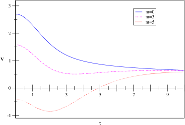
Figure 1: Potential V($\tau)$ for different values of $-k^{2}=m^{2}$

Thus, for sufficiently large $m^{2}$ the potential is negative and there will be normalizable modes, Figure 1. The WKB approximation consists in demanding that at the turning point $\tau_{o}$ , the exponential solution on one side matches the oscillatory solution on the other. The renormalizable modes are determined by the transcendental equation

$$\int_{0}^{\tau_{0}(m^{2})}{\sqrt{|V(x)|}}dx=\frac{3\pi}{4}+(n-1)\pi$$

where $n=1,2,3...$and $\tau_{0}$ is a root of $V(\tau_{0})=0.$ Solving this equation numerically we find the first eigenvalue

$$m^{2}_{0}=21.90$$

where the mass is measured in units of the conifold deformation $\epsilon^{4/3}.$

3.2 Exact numerical solution of supergravity equations

Equation (10) is an eigenvalue problem that can be solved exactly by a variety of numerical methods. The boundary condition at infinity is found by demanding normalizability of the states. Thus, we require that $\int|g(\tau)|^{2}dx^{10}$ converges and investigating the asymptotic behavior of the equation we find that at infinity $g(\tau)\sim\exp(-\frac{4}{3}\tau)$. Close to the origin we will demand the function to be smooth i.e $\left.\frac{dg(\tau)}{d\tau}\right|_{\tau=0}=0.$ Therefore, we want to find the eigenvalues $k^{2}$ for which there exits a solution of satisfying the boundary conditions discussed above. We choose to solve this problem using a shooting technique. This method is very accurate for low lying states but requires an initial guess for the eigenvalue. We used as initial guess the eigenvalue found in the previous section using a WKB approximation. The coefficients entering the equation, $A(\tau)$and $B(\tau),$ involve combinations of hyperbolic functions that make them extremely sensitive to accumulation of numerical error. In order to overcome this difficulty we calculate $A(\tau)$and $B(\tau)$ with 20 digits of precision . With this technique we find a very stable eigenvalue,

$$m^{2}(2^{++})=18.33.$$

We did not find any excited $2^{++*}$ state, it is possible that the excited states are too heavy for us to see them since our code was design to determine accurately the lowest mode.

4 Spectrum and Regge slope

The low-lying glueball masses for the KS model found by Cáceres and Hernández [6] and the one obtained in this work are shown in the following table,

State	$Mass^{2}/\epsilon^{4/3}$
$0^{++}$	9.78
$1^{--}$	14.05
$2^{++}$	18.33

Table 3: Glueball masses for the KS model.

The Chew-Frautschi plot for the glueball trajectory obtained with these values is shown in Figure 2. It is remarkable that the three states lie on a straight line. For large quantum numbers it is known that glueballs can be identified with spinning folded closed strings. In that approach a linear Regge trajectory is no surprise since it is built in the formalism. But in the present framework, where we identify masses with eigenvalues of equations of motion, there is no a priori reason for the eigenvalues to lie on a straight line. The fact that it is so is remarkable. The glueball Regge trajectory obtained from the KS model is

$$J=-2.2+0.23\,t$$

Lattice data for the intercept of the glueball trajectory is inconclusive. While Morningstar and Peardon find a negative intercept [15], Teper finds a positive one [17]. If the glueball trajectory is identified with the soft Pomeron then experimental data suggests the intercept is positive. But we do not pretend to compare the full Regge trajectory obtained here with experimental parameters. We do not know how to fix the scale $\epsilon^{2/3}$ and thus, any direct comparison is far fetched. Furthermore, as in [11], quantum corrections might turn out to be crucial to modify the intercept.

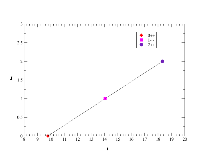
Figure 2: Glueball trajectory. The mass squared, $t$, is measured in units of $\frac{\epsilon^{4/3}}{g_{s}^{2}\alpha^{\prime 2}M^{2}}$.

5 Conclusions

We have calculated the mass of the spin 2 glueball in the Klebanov-Strassler background. We find $m^{2}(2^{++})=18.33\frac{\epsilon^{4/3}}{g_{s}^{2}\alpha^{\prime 2}M^{2}}$. We showed that the Regge trajectory obtained is linear with a slope of $0.23\,(\frac{g_{s}^{2}\alpha^{\prime 2}M^{2}}{\epsilon^{4/3}})$. Comparison of mass ratios with lattice results is in agreement within one sigma error. The intercept of the Regge trajectory found is negative. We expect that quantum corrections will modify the value of the intercept and will make the trajectory non-linear. It would be interesting to study this issue in detail.

Appendix A

In this appendix we will show some details of the derivation of (10). After expanding in spherical harmonics the equation to be solved is,

$$-\frac{1}{2}\nabla^{\lambda}\nabla_{\lambda}h_{ij}(\tau,\bar{x})\,+\frac{1}{2}\nabla^{l}\nabla_{i}h_{lj}(\tau,\bar{x})\,+\frac{1}{2}\nabla^{l}\nabla_{j}h_{li}(\tau,\bar{x})=\,\,\,\,\,\,\,\,\,\,\,\,\,\,\,\,\,\,\,\,\,\,\,\,\,\,\,\,\,\,\,$$

$$\left(\,\frac{g_{s}^{2}}{96}\,\left(\frac{1}{5}\mathcal{\star F}_{5}^{KS}\cdot\mathcal{\star F}_{5}^{KS}\right)\,-\left.\frac{g_{s}^{2}}{48}H_{3}^{KS}\cdot H_{3}^{KS}-\frac{1}{48}F_{3}^{KS}\cdot F_{3}^{KS}\right)h_{ij}(\tau,\bar{x})\right.$$ (A-1)

where $\bar{x}$ denotes worldvolume coordinates $(x_{1},x_{2},x_{3},x_{4}),\textrm{ $\tau$ is the radial coordinate and }$the covariant derivative is with respect to the metric

$$ds_{10}^{2} = h^{-1/2}(\tau)dx_{n}dx_{n}+h^{1/2}(\tau)ds_{6}^{2},$$ (A-2)

$$h(\tau)=(g_{s}M\alpha^{\prime})^{2}2^{2/3}\epsilon^{-8/3}I(\tau) I(\tau)\equiv\int_{\tau}^{\infty}dx\ \frac{(x\coth x-1)(\sinh(2x)-2x)^{1/3}}{\sinh^{2}x}$$

We will work in the basis $\{\tau,\,g^{1},\,g^{2},\,g^{3},\,g^{4},\,g^{5}\}$ where the deformed conifold metric is diagonal,

$${ds_{6}}^{2}=\frac{1}{2}\epsilon^{4/3}K(\tau)\left[\frac{1}{3K^{3}(\tau)}(d^{2}\tau+(g^{5})^{2})\right. + \cosh^{2}(\frac{\tau}{2})[(g^{3})^{2}+(g^{4})^{2}]$$ (A-3)

$$+ \left.\sinh^{2}(\frac{\tau}{2})[(g^{1})^{2}+(g^{2})^{2}]\rule{0.0pt}{17.07182pt}\right]$$

Note that the dimensionfull parameter $\epsilon$ and $g_{s}M\alpha^{\prime},$ appear in $h(\tau)$ and in the deformed conifold metric. Define $G_{ij}(\tau)$ such that $g_{ii}(\tau)=h(\tau)^{-1/2}G_{ii}(\tau)$ for $i=1...4$ and $g_{\mu\mu}(\tau)=h(\tau)^{1/2}\epsilon^{4/3}G_{\mu\mu}(\tau)$ for $\mu=5...10$. Explicitly,

$$G_{ii}(\tau)= \eta_{ii} i=1...4$$

$$G_{66}(\tau)= G_{55}(\tau)= \frac{1}{6K(\tau)^{2}}$$

$$G_{88}(\tau)= G_{77}(\tau)= \frac{1}{2}K(\tau)\cosh^{2}(\frac{\tau}{2})$$

$$G_{1010}(\tau)= G_{99}(\tau)= \frac{1}{2}K(\tau)\sinh^{2}(\frac{\tau}{2})$$

With this notation we obtain for the left hand side of (A-1),

$$-\frac{1}{2}\nabla^{\lambda}\nabla_{\lambda}h_{ij}(\tau,\bar{x})\,+\frac{1}{2}\nabla^{l}\nabla_{i}h_{lj}(\tau,\bar{x})\, + \frac{1}{2}\nabla^{l}\nabla_{j}h_{li}(\tau,\bar{x})=\frac{e^{ikx}}{g_{s}\alpha^{\prime}M\sqrt{I(\tau)}G_{55}(\tau)2^{1/3}}\left[-\frac{d^{2}h_{ij}(\tau)}{d\tau^{2}}\right.$$

$$- \left(\frac{d\ln I(\tau)}{d\tau}+\frac{d\ln G_{99}(\tau)}{d\tau}+\frac{d\ln G_{77}(\tau)}{d\tau}\right)\frac{dh_{ij}(\tau)}{d\tau}$$

$$+ \left.\left(\frac{g_{s}^{2}M^{2}\alpha^{\prime 2}G_{55}(\tau)}{2^{1/3}\epsilon^{4/3}}I(\tau)k^{2}-\frac{1}{4I(\tau)^{2}}\left(\frac{dI(\tau)}{d(\tau)}\right)^{2}\right)\right]h_{ij}(\tau)$$

The five form and three form terms are,

$$\left(\frac{1}{5}\mathcal{\star F}_{5}^{KS}\cdot\mathcal{\star F}_{5}^{KS}\right)h_{ij}(\tau)=-\frac{e^{ikx}}{g_{s}\alpha^{\prime}M\sqrt{I(\tau)}G_{55}(\tau)2^{1/3}}\left(\frac{2^{5/3}l(\tau)^{2}}{I(\tau)^{2}K(\tau)^{4}(\cosh^{2}\tau-1)^{2}}\right)h_{ij}(\tau)$$

(A-5)

$$-\left(\frac{g_{s}^{2}}{48}H_{3}^{KS}\cdot H_{3}^{KS}+\frac{1}{48}F_{3}^{KS}\cdot F_{3}^{KS}\right)h_{ij}(\tau) = \frac{e^{ikx}}{g_{s}\alpha^{\prime}M\sqrt{I(\tau)}G_{55}(\tau)}$$

$$\left\{\frac{1}{8I(\tau)}\left[\frac{-1}{G_{77}^{2}(\tau)}\right.\left(\left(\frac{dk(\tau)}{d\tau}\right)+(1\!-F(\tau))^{2}\right)\right.$$

$$- \frac{2}{G_{77}(\tau)G_{99}(\tau)}\left(\left(\frac{dF(\tau)}{d\tau}\right)^{2}+\frac{1}{4}(k(\tau)-f(\tau))^{2}\right)$$

$$- \left.\left.\frac{1}{G_{99}^{2}(\tau)}\left(F(\tau)^{2}+\left(\frac{df(\tau)}{d\tau}\right)^{2}\right)\right]\right\}h_{ij}(\tau)$$

Putting together equations (LABEL:eq:explicitricci),(A-5) and (LABEL:eq:threeformterm) we obtain,

$$\frac{d^{2}}{d\tau^{2}}h_{ij}\left(\tau\right)+A\left(\tau\right)\frac{d}{d\tau}h_{ij}\left(\tau\right)+\left(B\left(\tau\right)+\frac{g_{s}^{2}\alpha^{\prime 2}M^{2}}{2^{1/3}\epsilon^{4/3}}I(\tau)G_{55}(\tau)k^{2}\right)h_{ij}\left(\tau\right)=0$$

with

$$A(\tau)=\frac{d\ln(G_{99}(\tau))}{d\tau}+\frac{d\ln(G_{77}(\tau))}{d\tau}+\frac{d\ln I(\tau)}{d\tau}$$

and

$$B(\tau) = \frac{-2^{(1/3)}}{8I(\tau)G_{77}(\tau)^{2}}(1-F(\tau))^{2}-(\frac{d}{d\tau}k(\tau))^{2}-\frac{2^{1/3}}{16G_{77}(\tau)G_{99}(\tau)}(k(\tau)-f(\tau))^{2}+$$

$$\frac{2^{1/3}}{4}(\frac{d}{d\tau}F(\tau))^{2}-\frac{2^{1/3}}{8I(\tau)G_{99}(\tau)^{2}}((\frac{d}{d\tau}f(\tau))^{2}+F(\tau)^{2})$$

$$+\frac{1}{4I(\tau)^{2}}\left(\frac{dI(\tau)}{d\tau}\right)^{2}-\frac{2^{5/3}l(\tau)^{2}}{I(\tau)^{2}K(\tau)^{4}(\cosh^{2}\tau-1)^{2}}.$$

The explicit form of $A(\tau)$ and $B(\tau)$ in terms of hyperbolic functions is obtained by substituting the definitions of section (2) in the expressions above.

References

• [1] J. M. Maldacena, “The large N limit of superconformal field theories and supergravity,” Adv. Theor. Math. Phys. 2 (1998) 231–252, hep-th/9711200.
• [2] S. S. Gubser, I. R. Klebanov, and A. M. Polyakov, “Gauge theory correlators from non-critical string theory,” Phys. Lett. B428 (1998) 105–114, hep-th/9802109.
• [3] J. Polchinski and M. J. Strassler, “The string dual of a confining four-dimensional gauge theory,” hep-th/0003136.
• [4] I. R. Klebanov and M. J. Strassler, “Supergravity and a confining gauge theory: Duality cascades and chisb-resolution of naked singularities,” JHEP 08 (2000) 052, hep-th/0007191.
• [5] J. M. Maldacena and C. Nuñez, “Towards the large N limit of pure ${\mathcal{N}}=1$ super Yang Mills,” Phys. Rev. Lett. 86 (2001) 588–591, hep-th/0008001.
• [6] E. Cáceres and R. Hernández, “Glueball masses for the deformed conifold theory,” Phys. Lett. B504 (2001) 64–70, hep-th/0011204.
• [7] M. Krasnitz, “A two point function in a cascading n = 1 gauge theory from supergravity,” hep-th/0011179.
• [8] T. Sakai and J. Sonnenschein, “Probing flavored mesons of confining gauge theories by supergravity,” JHEP 09 (2003) 047, hep-th/0305049.
• [9] P. Collins, An Introduction to Regge Theory. Cambridge University Press, 1977.
• [10] P. L. S. Donnachie, G. Bosch and O. Nachtmann, Pomeron Physics and QCD. Cambridge University Press, 2002.
• [11] L. Pando Zayas, J. Sonnenschein, and D. Vaman, “Regge trajectories revisited in the gauge/string correspondence,” hep-th/0311190.
• [12] G. F. Chew and S. C. Frautschi, “Principle of equivalence for all strongly interacting particles within the S matrix framework,” Phys. Rev. Lett. 7 (1961) 394–397. G. F. Chew and S. C. Frautschi, “Regge trajectories and the principle of maximum strength for strong interactions,” Phys. Rev. Lett. 8 (1962) 41–44.
• [13] B. Lucini and M. Teper, “SU(N) gauge theories in four dimensions: Exploring the approach to $N=\infty$,” JHEP 06 (2001) 050, hep-lat/0103027.
• [14] C. Morningstar and M. J. Peardon, “Simulating the scalar glueball on the lattice,” nucl-th/0309068.
• [15] C. J. Morningstar and M. J. Peardon, “The glueball spectrum from an anisotropic lattice study,” Phys. Rev. D60 (1999) 034509, hep-lat/9901004.
• [16] C. Herzog, I. Klebanov, and O. P., “D-branes on the conifold and n=1 gauge/gravity dualitites,” hep-th/0205100.
• [17] M. J. Teper, “Glueball masses and other physical properties of SU(N) gauge theories in d = 3+1: A review of lattice results for theorists,” hep-th/9812187.