DEDICATED TO THE MEMORY OF MARIA

IFT-UAM/CSIC-03-54

hep-th/0402042

Hunting for the New Symmetries
in
Calabi-Yau Jungles
Guennadi Volkov

IFT UAM, Madrid, Spain

Abstract

It was proposed that the Calabi-Yau geometry can be intrinsically connected with some new symmetries, some new algebras. In order to do this it has been analyzed the graphs constructed from K3-fibre $CY_{d}$ ($d\geq 3$) reflexive polyhedra. The graphs can be naturally get in the frames of Universal Calabi-Yau algebra (UCYA) and may be decode by universal way with the changing of some restrictions on the generalized Cartan matrices associated with the Dynkin diagrams that characterize affine Kac-Moody algebras. We propose that these new Berger graphs can be directly connected with the generalizations of Lie and Kac-Moody algebras.

1 Introduction

Now it becomes more and more reasonable that the Standard Model could have an intrinsic link with a more fundamental symmetry, than the finite Lie symmetries. Of course, this fundamental symmetry should generalize the symmetries of the Standard Model, since a lot of experimental data confirm its. The main argument to think about a new symmetry with some extraordinary properties is that the symmetries linked to the finite Lie groups are not sufficient for a description of many parameters and features of the Standard Model. Therefore hyphotetical symmetry could be a natural generalization of the finite Lie symmetries with stronger constraints leading to diminishing the number of free parameters. In principle, in (super)string approach we already have the interesting example of the generalization of finite Lie algebras by an infinite-dimensional affine algebra with a central charge. Since a finite-dimensional simple algebra has only trivial central extensions, at first one should construct a loop algebra, which is a Lie algebra associated to loop groups. Generally, a loop group is a group of mapping from manifold $M$ to a Lie group $G$. Concretely it was considered a case where the manifold is the unit circle and $G$ is an $n\times n$ matrix Lie group. So one can see a way of construction of new algebras, which have a very closed link to the geometry. A loop algebra is an infinite-dimensional algebra which can already have non-trivial central extensions having some important implications in physics. Thus affine Kac-Moody algebras were constructed from loop algebras built on finite-dimensional simple Lie algebras. Superstring theory intrinsically contains a number of infinite-dimensional algebraic symmetries, such as the Virasoro algebra associated with conformal invariance and affine Kac-Moody algebras [19]. Certain string symmetries may be related to generalizations of Kac-Moody algebras (KMA), such as hyperbolic and Borcherds algebras [5].

One of the most important success of such implications was connected with a graduating of representations, what is given in affine algebra by its level [20] ( see some superstring models based on KMA in [28]).

Historically, a more traditional way to search for new fundamental symmetries lyes in the study of new geometrical objects of high dimensions. Last 20 years the old symmetrical geometry was intensively used in supergravity in Kaluza-Klein scenarium. The superstring theories already are connected closely with some new manifolds, which are already non-symmetric. The compactification of the heterotic $E(8)\times E(8)$ superstring discovered for physics the 6-dimensional Calabi-Yau space, having the $SU(3)$ group of holonomy [11]. In mathematics, based on the holonomy principle in 1955 Berger [7] suggested the classification of non-symmetrical spaces. As result of such classification there are some infinite series with $SO(n)$, $U(n)$, $SU(n)$, $Sp(n)\times Sp(1)$, $Sp(n)$ groups of holonomy and, also, some exceptional spaces with holonomy $G(2)$, $Spin(7)$, $Spin(16)$. For our goal there can be a special interest to study the $CY_{n}$ spaces with $n=2,3,...$.

It was luckly happened that the $K3\equiv CY_{2}$ spaces with its rich singularity structure are closely connected to the affine Lie symmetries. This link of $CY_{2}$ spaces with $A_{r}^{(1)}$, $D_{r}^{(1)}$, $E_{6}^{(1)}$, $E_{7}^{(1)}$, $E_{8}^{(1)}$ algebras can be explained by the creapent resolution of specific quotient singular structures of considered spaces like as Kleinian-Du-Val singularities ${{\bf C}^{2}/G}$[15], where $G$ is a discrete subgroup of $SU(2)$. For example, the creapent resolution of the ${{\bf C}^{2}/Z_{n}}$ singularity gives for rational, i.e., genus zero, (-2)-curves, an intersection matrix that coincides with the ${-A_{n-1}}$ Cartan matrix. Also, for elliptic fibre $K3$ spaces which can be written in Weierstrass form there exist the ADE classification of degenerations of the fibres [26, 8].

Calabi-Yau spaces may be characterized geometrically by reflexive Newton polyhedra, which have been enumerated systematically. More recently, it has been realized that reflexive polyhedra are related algebraically via what we term the Universal Calabi-Yau Algebra (UCYA) that includes ternary and higher-order operations as well as the binary operations employed in the CLA, KMA and Virasoro algebra.

The UCYA is particularly well suited for exploring fibrations of Calabi-Yau spaces, which are visible as lower-dimensional slices through higher-dimensional reflexive polyhedra, such as the example shown in Fig. 1. One can the elliptic fibration - described by the planar polyhedron denoted by hexagonal symbols - of a K3 space - whose reflexive polyhedron includes the additional points denoted by square and circular symbols.

The left square points and right circular points correspond to the extensions of two reflexive weight vectors, what one can see on the Fig.  1. According to binary operation in UCYA the sum of these two extended vector gives a ${\vec{k}}_{4}$ reflexive vector, describing the $CY_{2}=K3$ manifold. The UCYA provides analogous decompositions of fibrations in higher-dimensional Calabi-Yau spaces, as we discuss later in this paper.

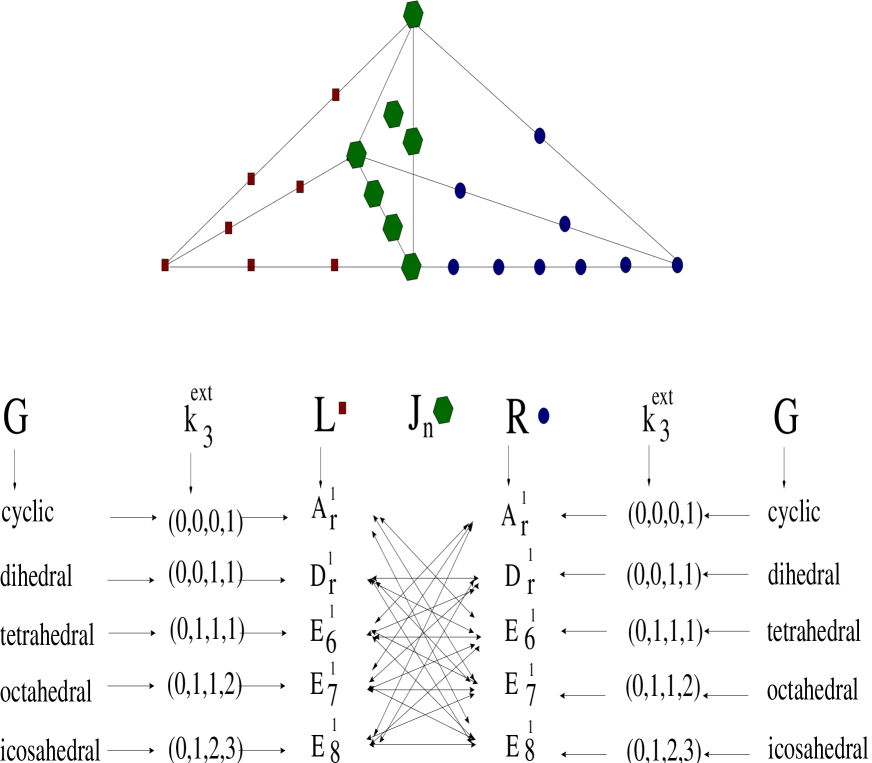
Figure 1: Example of an elliptic fibration of a K3 space, represented by a reflexive Newton polyhedron whose left and right part are characterized by two reflexive weight vectors, respectively. The square symbols on the left form a graph identical with the Dynkin diagram for the Cartan-Lie algebra $E_{6}^{(1)}$ and the circular symbols on the right form the Dynkin diagram of E${}^{1}_{8}$. Other examples of the correspondence between reflexive weight vectors and the Dynkin diagrams for the ADE series appearing in elliptic fibrations of K3 spaces are listed below.

One of the remarkable features of Fig. 1 is that the set of square symbols on the left constitute a graph that is isomorphic with the Dynkin diagram for $E_{6}{(1)}$, and the circular symbols on the left constitute the Dynkin diagram for E${}^{1}_{8}$. This is not an isolated example. Indeed, all the elliptic fibrations of K3 spaces found using the UCYA feature this decomposition into a pair of graphs that can be interpreted as Dynkin diagrams. And this can be confirmed in a singular limit of the K3 space, when there appears a gauge symmetry whose Cartan-Lie algebra corresponds to the Dynkin diagram seen as a graph on one side of Fig. 1.

In general, the rich singularity structures of K3 $\equiv$ CY₂ spaces are closely connected to the affine Cartan-Lie symmetries A${}_{r}^{(1)}$, D${}_{2r}^{(1)}$, E${}_{6}^{(1)}$, E${}_{7}^{(1)}$ and E${}_{8}^{(1)}$ via the crepant resolution of specific quotient singular structures such as the Kleinian-Du-Val singularities ${{\bf C}^{2}/G}$ [15], where $G$ is a discrete subgroup of SU(2). For example, the crepant resolution of the ${{\bf C}^{2}/Z_{n}}$ singularity gives for rational, i.e., genus-zero, (-2) curves an intersection matrix that coincides with the -A_n-1 Cartan matrix. Also, in the case of K3 spaces with elliptic fibres which can be written in Weierstrass form, there exists and ADE classification of degenerations of the fibres [26, 8].

The UCYA provides a direct algebraic relation between such K3 = CY₂ spaces and the CY₃ spaces with SU(3) holonomy that came to prominence as manifolds for compactifying the heterotic E(8) $\times$ E(8) string theory [11]. The K3 and CY₃ spaces are just two examples of an infinite series with SU(n) holonomy. We have shown previously how the UCYA can be used to generate and interrelate the generalized $CY_{n}$ spaces with $n=2,3,...$.

The purpose of this paper is to explore generalizations of the affine Dynkin graphs associated with the ADE classification of elliptic fibrations of $CY_{d}$ spaces with $d\geq 2$ [1, 3, 4] illustrated in Fig. 1,2 and Tables 1,2. From studying of new graphs in Newton polyhedra of $CY_{d}$-( $d\geq 3$) we would like to analyse a possibility to find an non-trivial extension of CLA and KMA algebras:

$${\it Cartan-Lie\,\,algebras\,\rightarrow\,Kac-Moody\,\,affine\,\,algebras\,\rightarrow\,Universal\,\,algebras\,\,?}$$ (1)

Generalizations of the elliptic fibration shown there, such as K3 fibrations of higher CY_n spaces, reveal some types of generalization. The analysis of the all third line has been given in [1, 2, 3, 4] and we illustrate also here in two tables 1, 2 later. Our main goal to transfer our experience from the third line on the fourth line, points of which correspond to K3-fibre $CY_{d}$ with $d\geq 3$. We really discuss some cases, three cases are again connected with three set of RWVs of different dimensions, $\{\vec{k}_{1}=(1)\}$,$\{\vec{k}_{2}=(11)\}$ and $\{\vec{k}_{3}=(111),(112),(123)\}$, participating in creation of $K3$ fibre, and the other case is connected with K3-vectors, $\{{\vec{k}}_{4}=(1,1,1,1),(1113),...\}$. Just as Dynkin graphs correspond to Lie algebras via the imposition of certain conditions on the elements, determinants and minors of $r\times r$ Cartan matrices, and the generalized Dynkin diagrams for affine Kac-Moody algebras can be obtained by generalizing these conditions, so the new graphs we find in CY_d fibrations can be obtained by further generalizations of these conditions.

We find it interesting already that these graphs can be derived in such a way. The nature of any underlying algebraic structure remains more obscure, though we present some hints and suggestions for future work.

Elliptic fibre $CY_{d}$-polyhedra consist from d-types of regular graphs, which coincide with Dynkin diagrams. On the third slope line, $n=r+2$, on the arity-dimension plot the number $d$ ($n=d+2$) is the complex dimension of CY, coincide with number of the arity, $d=r$, coincide with the number of the copies of Dynkin diagrams. For K3 we illustrate later in the table with the 13-eldest vectors, and for $CY_{3}$- 27 eldest cases. In these cases one can see directly a correspondence between these 5- vectors and ADE graphs. The fig. 1, 2 illustrate the K3 case.

2 The Arity-Dimension Stucture of UCYA and Dynkin Graphs in Elliptic Polyhedra.

One of the main results in the Universal Calabi-Yau Algebra (UCYA) is that the reflexive weight vectors (RWVs) $\vec{k_{n}}$ of dimension $n$ can obtained directly from lower-dimensional RWVs $\vec{k_{1}},\ldots,\vec{k_{n-r+1}}$ by algebraic constructions of arity $r$ [1, 2, 3, 4]. As an example of an arity $r=2$ construction, first two $(n-1)$-dimensional RWVs ${\vec{k}}_{n-1}$ and ${\vec{l}}_{n-1}$ (which can be taken the same) can be used to obtain two new extended $n$-dimensional vectors,

$${\vec{k}}_{n}^{(ex)} = (k_{1},0|k_{2},\ldots,k_{n-1}),$$

$${\vec{l}}_{n}^{(ex)} = (0,l_{1}|l_{2},\ldots,l_{n-1}).$$ (2)

Then, using the composition rule of arity $r=2$, one can obtain from these two good extended vectors a new $n$-dimensional RWV:

$${\vec{p}}_{n}={\vec{k}}_{n}^{(ex)}+{\vec{l}}_{n}^{(ex)}=(k_{1},l_{1}|k_{2}+l_{2},\ldots,k_{n-1}+l_{n-1}),$$ (3)

which originates a chain of $n$-dimensional RWVs (Compare UCYA to theory of operads  [27]).

This arity-2 composition rule of the UCYA gives complete information about the $(d-1)$-dimensional fibre structure of $CY_{d}$ spaces, where $d=n-2$. For example, in the K3 case, 91 of the total of 95 RWVs $\vec{k_{4}}$ can be obtained by such arity-2 constructions out of just five RWVs of dimensions 1,2 and 3, namely

$$\vec{k_{1}}=(1)[1],\qquad \rightarrow \qquad A_{r}^{(1)}$$

$$\vec{k_{2}}=(1,1)[2],\qquad \rightarrow \qquad D_{r}^{(1)}$$

$$\vec{k_{3}}=(1,1,1)[3],\qquad \rightarrow \qquad E_{6}^{(1)}$$

$$\vec{k_{3}}=(1,1,2)[4],\qquad \rightarrow \qquad E_{7}^{(1)}$$

$$\vec{k_{3}}=(1,2,3)[6]\qquad \rightarrow \qquad E_{8}^{(1)}$$

as seen in Fig. 3. The 91 corresponding K3 reflexive polyhedra can be organized in 22 chains, having the natural link with Betti-Hodge numbers of K3, $b_{2}=22$.

This coincidence for $CY_{1}$ and $CY_{2}$ in UCYA was happened naturally, since $CY_{1}$ (complex torus) is one topological object having in the intersection two $S^{1}$, and $K3$ is also one topological object consisting of 22 $CP^{1}$. For $CY_{3}$ situation is a little bit more complicated, because topologically there are many $CY_{3}$, but also, the number of two-arity chains, 4242, has an intriguing expansion: $4242=2\cdot 21\cdot 101$. So, the other important success of UCYA is that it is naturally connected to the invariant topological numbers, and therefore it gives correctly all the double-, triple-, and etc. intersections, and, correspondingly, all graphs, which are connected with affine algebras.

It was shown [10, 13, 21, 25] in the toric-geometry approach how the Dynkin diagrams of affine Cartan-Lie algebras appear in reflexive K3 polyhedra [6]. Moreover, it was found in [1], using examples of the lattice structure of reflexive polyhedra for $CY_{n}$: $n\geq 2$ with elliptic fibres that there is an interesting correspondence [1, 3, 4] between the five basic RWVs (LABEL:fivevectors) and Dynkin diagrams for the five ADE types of Lie algebras: A, D and E_6,7,8 (see LABEL:fivevectors). For example, these RWVs are constituents of composite RWVs for K3 spaces, and the corresponding K3 polyhedra can be directly constructed out of certain Dynkin diagrams, as illustrated in Fig. 1. In each case, a pair of extended RWVs have an intersection which is a reflexive plane polyhedron, and one vector from each pair gives the left or right part of the three-dimensional reflexive polyhedron, as discussed in detail in [1].

One can illustrate this correspondence on the example of RWVs, $\vec{k_{3}}=(k_{1},k_{2},k_{3})[d_{\vec{k}}]=(111)[3],(112)[4],(123)[6]$, for which we show how to build the $E_{6}^{(1)}$, $E_{7}^{(1)}$, $E_{8}^{(1)}$ Dynkin diagrams, respecrtively. Let take the vector $\vec{k_{3}}=(111)[3]$. To construct the Dynkin diagram one should start from one common node, $V^{0}$, which will give start to n=3 (= dimension of the vector) line-segments. To get the number of the points-nodes $p$ on each line one should divide $d_{\vec{k}}$ on $k_{i}$, $i=1,2,3$, so $p_{i}=d_{\vec{k}}/k_{i}$ ( here we considere the cases when all divisions are integers). One should take into account, that all lines have one common node $V^{0}$. The numbers of the points equal to $n\cdot(d_{\vec{k}}/k_{i}-1)+1$. Thus, one can check, that for all these three cases there appear the $E_{6}^{(1)}$, $E_{7}^{(1)}$, $E_{8}^{(1)}$ graphs, respectively. Moreover, one can easily see how to reproduce for all these graphs the Coxeter labels and the Coxeter number. Firstly, one should prescribe the Coxeter label to the comon point $V^{0}$. It equals to $max_{i}\{p_{i}\}$. So in our three cases the maximal Coxeter label, prescribing to the common point $V^{0}$, is equal $3,4,6,$ respectively. Starting from the Coxeter label of the node $V^{0}$, one can easily find the Coxeter numbers of the rest points in each line. Note that this rule will help us in the cases of higher dimensional $CY_{d}$ with $d\geq 3$, for which one can easily represent the corresponding polyhedron and graphs without computors.

Similarly, the huge set of five-dimensional RWVs $\vec{k_{5}}$ in 4242 CY₃ chains of arity 2 can be constructed out of the five RWVs already mentioned plus the 95 four-dimensional K3 RWVs $\vec{k_{4}}$, as summarized in Fig. 3). In this case, reflexive 4-dimensional polyhedra are also separated into three parts: a reflexive 3-dimensional intersection polyhedron and ‘left’ and ‘right’ graphs. By construction, the corresponding CY₃ spaces are seen to possess K3 fibre bundles.

We illustrate the case of one such arity-2 K3 example, shown in Fig. 2. In this case, a reflexive K3 polyhedron is determined by the two RWVs ${\vec{k}}_{1}=(1)[1]$ and ${\vec{k}}_{3}=(1,2,3)[6]$. As one can see, this K3 space has an elliptic Weierstrass fibre, and its polyhedron, determined by the RWV ${\vec{k}}_{4}=(1,0,0,0)+(0,1,2,3)=(1,1,2,3)[7]$, can be constructed from two diagrams, $A_{6}^{(1)}$ and $E_{8}^{(1)}$, depicted to the left and right of the triangular Weierstrass skeleton. The analogous arity-2 structures of all 13 eldest K3 RWVs [1]. One can see the correspondence of 5 RWVs and ADE series of affine Lie algebras in the Table 1.

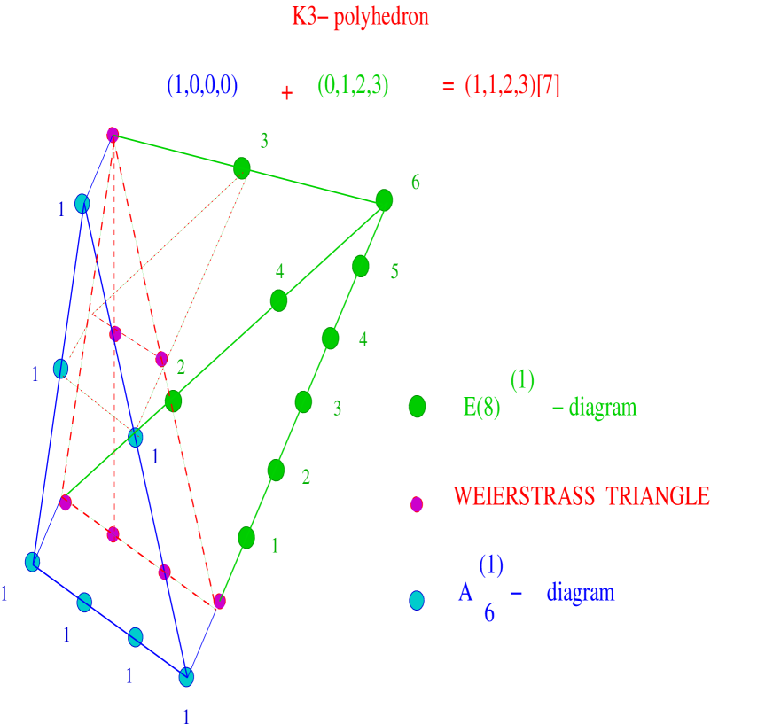
Figure 2: The decomposition of the the K3 polyhedron determined by ${\vec{k}}_{4}=(1,1,2,3)[7]$ with an elliptic Weierstrass intersection/projection gives the two Dynkin diagramms for $A_{6}^{(1)}$ and $E(8)^{(1)}$.

Table 1: The eldest vectors for all $S_{2}$-symmetric chains of $k3$ hypersurfaces and two Dynkin graphs in corresponding polyhedra.

${N}$	$L-R$	$I$	${{\vec{k}}_{i}(eldest)}$	$Cox-Dyn$	$P_{0}section$
${1}$	$(0111)\bigcap(1000)$	$(10,4)$	$(11|11)$	$(E_{6})(A)$	$(1,3,|0,0)$
${2}$	$(0011)\bigcap(1100)$	$(9,5)$	$(11|11)$	$(D)^{2}$	$(2,2,|0,0)$
${3}$	$(1011)\bigcap(1001)$	$(9,5)$	$(11|12)$	$(E_{6})(D)$	$(3,2,|0,0)$
${4}$	$(0112)\bigcap(1000)$	$(9,5)$	$(11|12)$	$(E_{7})(A)$	$(1,4,|0,0)$
${5}$	$(0111)\bigcap(1011)$	$(10,4)$	$(11|22)$	$(E_{6})^{2}$	$(3,3,|0,0)$
${6}$	$(0112)\bigcap(1001)$	$(9,5)$	$(11|13)$	$(E_{7})(D)$	$(2,4,|0,0)$
${7}$	$(1012)\bigcap(0111)$	$(8,6)$	$(11|23)$	$(E_{7})(E_{6})$	$(4,3,|0,0)$
${8}$	$(0123)\bigcap(1000)$	$(7,7)$	$(11|23)$	$(E_{8})(A)$	$(1,6,|0,0)$
${9}$	$(0112)\bigcap(1012)$	$(9,5)$	$(11|24)$	$(E_{7})^{2}$	$(4,4,|0,0)$
${10}$	$(0123)\bigcap(1001)$	$(7,7)$	$(11|24)$	$(E_{8})(D)$	$(2,6,|0,0)$
${11}$	$(1023)\bigcap(0111)$	$(7,7)$	$(11|34)$	$(E_{8})(E_{6})$	$(6,3,|0,0)$
${12}$	$(1023)\bigcap(0112)$	$(7,7)$	$(11|35)$	$(E_{8})(E_{7})$	$(6,4,|0,0)$
${13}$	$(0123)\bigcap(1023)$	$(7,7)$	$(11|46)$	$(E_{8})^{2}$	$(6,6,|0,0)$

Similarly, taking into account the composition rule of arity 3 in UCYA from three (two or one) reflexive $(n-2)$-dimensional weight vectors, ${\vec{k}}_{n-2}$,${\vec{l}}_{n-2}$,${\vec{m}}_{n-2}$, (of course, some of these RWVs or all three RWVs, ${\vec{k}}_{n-1}$, ${\vec{l}}_{n-1}$, ${\vec{m}}_{n-1}$, can be equal), one can find the $(n)$-dimensional reflexive weight-vector

$${\vec{p}}_{n}=(k_{1},l_{1},m_{1}|k_{2}+l_{2}+m_{2},\ldots,k_{n-2}+l_{n-2}+m_{n-2})$$ (5)

and then one can construct all chain, for which ${\vec{p}}_{n}$ is the eldest vector. Similarly to situation with arity 2, the UCYA with arity 3 gives the complete information about (d-2)- dimensional fibre structure of d-dimensional Calabi-Yau spaces in this chain. And this process can be continued till the natural final (see Fig. 3.)

The set of $\vec{k_{5}}$- RWVs, corresponding to the elliptic fibre Calabi-Yau, in UCYA can be got with arity-3,$r=3$ ı.e. they can be constructed again only from already well-known five reflexive vectors of dimensions, 1,2,3. In this case the reflexive polyhedra can be considered from 4-parts: plane reflexive polyhedron in triple intersection and three graphs. The corresponding Calabi-Yau will be already the elliptic fibre-bundles. Such composite structure of RWVs and fibre structure of $CY_{n}$ is illustrated on the arity-dimension plot 3.

The corresponding reflexive polyhedra of elliptic fibre $CY_{3}$ ($CY_{d}$) will construct from $3$ ($d$) Dynkin diagramms of all five possible affine $A,D,E_{6},E_{7},E_{8}$-types based on the elliptic fibre-graph [4]. One can illustrate this by a list of some elliptic fibre $CY3$ giving in the following table 2:

Table 2: The eldest vectors for all $S_{3}$-symmetric chains of $CY_{3}$ hypersurfaces.

${N}$	${{\vec{k}}_{i}(eldest)}$	$h^{2,1}$	$h^{1,1}$	$V$	$V^{*}$	$Cox-Dyn$	$P_{0}$
${1}$	$(1,1,1|1,1)$	$101$	$1$	$5$	$5$	$(E_{6})(A)^{2}$	$(3,1,1|0,0)$
${2}$	$(1,1,1|1,2)$	$103$	$1$	$5$	$5$	$(E_{7})(A)^{2}$	$(4,1,1|0,0)$
${2^{\prime}}$	$(1,1,1|1,2)$	$103$	$1$	$5$	$5$	$(E_{6})(D)(A)$	$(3,2,1|0,0)$
${3}$	$(1,1,1|1,3)$	$122$	$2$	$8$	$6$	$(E_{6})(D)^{2}$	$(3,2,2|0,0)$
${4}$	$(1,1,1|1,4)$	$149$	$1$	$5$	$5$	$(E_{7})(D)^{2}$	$(4,2,2|0,0)$
${5}$	$(1,1,1|2,2)$	$95$	$2$	$9$	$6$	$(E_{6})^{2}(A)$	$(3,3,1|0,0)$
${6}$	$(1,1,1|2,3)$	$106$	$2$	$8$	$6$	$(E_{6})^{2}(D)$	$(3,3,2|0,0)$
${6^{\prime}}$	$(1,1,1|2,3)$	$106$	$2$	$8$	$6$	$(E_{7})(E_{6})(A)$	$(4,3,1|0,0)$
${6^{\prime\prime}}$	$(1,1,1|2,3)$	$106$	$2$	$8$	$6$	$(E_{8})(A)^{2}$	$(6,1,1|0,0)$
${7}$	$(1,1,1|2,4)$	$123$	$3$	$9$	$6$	$(E_{7})(E_{6})(D)$	$(4,3,2|0,0)$
${7^{\prime}}$	$(1,1,1|2,4)$	$123$	$3$	$9$	$6$	$(E_{8})(D)(A)$	$(6,2,1|0,0)$
${8}$	$(1,1,1|2,5)$	$145$	$1$	$5$	$5$	$(E_{7})^{2}(D)$	$(4,4,2|0,0)$
${8^{\prime}}$	$(1,1,1|2,5)$	$145$	$1$	$5$	$5$	$(E_{8})(D)^{2}$	$(6,2,2|0,0)$
${9}$	$(1,1,1|3,3)$	$112$	$4$	$5$	$5$	$(E_{6})^{3}$	$(3,3,3|0,0)$
${10}$	$(1,1,1|3,4)$	$126$	$4$	$10$	$7$	$(E_{7})(E_{6})^{2}$	$(4,3,3|0,0)$
${10^{\prime}}$	$(1,1,1|3,4)$	$126$	$4$	$10$	$7$	$(E_{8})(E_{6})(A)$	$(6,3,1|0,0)$
${11}$	$(1,1,1|3,5)$	$144$	$4$	$10$	$7$	$(E_{7})^{2}(E_{6})$	$(4,4,3|0,0)$
${11^{\prime}}$	$(1,1,1|3,5)$	$144$	$4$	$10$	$7$	$(E_{8})(E_{7})(A)$	$(6,4,1|0,0)$
${12}$	$(1,1,1|,3,6)$	$165$	$3$	$5$	$5$	$(E_{7})^{3}$	$(4,4,4|0,0)$
${12^{\prime}}$	$(1,1,1|,3,6)$	$165$	$3$	$5$	$5$	$(E_{8})(E_{7})(D)$	$(6,4,2|0,0)$
${13}$	$(1,1,1|4,5)$	$154$	$4$	$7$	$6$	$(E_{8})(E_{6})^{2}$	$(6,3,3|0,0)$
${14}$	$(1,1,1|4,6)$	$173$	$5$	$9$	$6$	$(E_{8})^{2}(A)$	$(6,6,1|0,0)$
${14^{\prime}}$	$(1,1,1|4,6)$	$173$	$5$	$9$	$6$	$(E_{8})(E_{7})(E_{6})$	$(6,4,3|0,0)$
${15}$	$(1,1,1|4,7)$	$195$	$3$	$7$	$6$	$(E_{8})(E_{7})^{2}$	$(6,4,4|0,0)$
${15^{\prime}}$	$(1,1,1|4,7)$	$195$	$3$	$7$	$6$	$(E_{8})^{2}(D)$	$(6,6,2|0,0)$
${16}$	$(1,1,1|5,7)$	$208$	$4$	$7$	$6$	$(E_{8})^{2}(E_{6})$	$(6,6,3|0,0)$
${17}$	$(1,1,1|5,8)$	$231$	$3$	$7$	$6$	$(E_{8})^{2}(E_{7})$	$(6,6,4|0,0)$
${18}$	$(1,1,1|6,9)$	$272$	$2$	$5$	$5$	$(E_{8})^{3}$	$(6,6,6|0,0)$

So the main discrepancy between this table and $K3$ case is that in $CY_{3}$ reflexive polyhedra will appear three Dynkin diagrams of $A-$,$D-$,$E_{6}-,E_{7}-,E_{8}-$ types. This analogy can be easily prolongated to the $CY_{d}$ polyhedra with $d=4,5,...$.

3 Affine graphs from the lattice of reflexive $CY_{d}\,\,(d\geq 3)$ polyhedra.

Now one can expect that the next step in studying of $K3$-fibre $CY_{3}$ $Y_{4},...$ spaces can give a possibility to find new graphs with new but universal regularity in its structure, which could indicate about some new algebras and … symmetries.

A hope to find these symmetries is linked to a possible existence of some new universal algebras, which could be considered as a natural generalization/ extension of Cartan-Lie algebras. The string theory and conformal theory [12, 16] already gave us one wonderfull example of extension of the finite simple Cartan-Lie algebras towards non-simple affine Kac-Moody algebras with non-trivial central charge. We already have got a lot of confirmations that $K3$ geometry has very closed link with affine Kac-Moody algebras. So, it is very natural to suggest that the geometry of $CY_{d}$ ($d\geq 3$) can help us to build a new algebra, which should be an extension of affine Kac-Moody algebras and, even more, an extension of Lie algebras. Actually, if the Lie algebras are based only on the binary composition law, new algebras could be universal, i.e. contain itself some n-ary composition multiplications, for example, binary, ternary and etc. This motivation has been supported by the completeness description of Calabi-Yau spaces with all its non-trivial fibre structures in universal Calabi-Yau algebra (UCYA) [1] which contains some fixed number of the composition operations $binary,ternary,...$,$\omega_{r}-ary$ with $\omega_{max}=n=d+2$ (see figure 3). UCYA is not a Lie algebra. Its composition laws of multiplications have algebraically a more closed link with theory of operads [27], and geometrically with exact sequences in theory of relative homology groups^∗. But on the example of applying of UCYA we have got a chance to understand how it is working algebra with many composition laws.

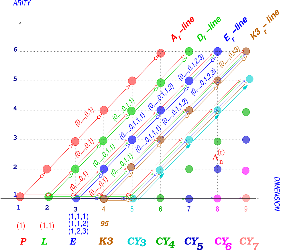
Figure 3: The arity-dimension plot, illustrating the normal expansion of RWVs by adding zero components to lower-dimensional vectors. For each dimension $n$ and arity $r$, it is possible to reconstruct a set of extended vectors.  [1, 2].

According to the third slope line, $n=r+2$, on the arity-dimension plot we have studied a correspondence between the five reflexive weight-vectors,$\vec{k}_{1}$, $\vec{k}_{2}$, $\vec{k}_{3}$ and (ADE)-graphs, which can be got from all elliptic fibre $CY_{d}$-polyhedra, and the number of the copies of Dynkin diagrams directly equal to $d$ (see Figure 3)). The next natural step is to study a correspondence between the RWVs and graphs of $CY_{3}$ on the fourth slope-line, $n=r+3$, which describes the K3-fibre Calabi-Yau spaces with arity $\omega_{r}\geq 2$. Really, we start to study a correspondence between $1+1+3+95$ RWVs in the case of $CY_{3}$ spaces with arity 2, and this helps us to understand also the lattice structure of the graphs on all fourth slope-line, $n=r+3$ Moreover, the investigation of the elliptic- and K3- fibre $CY_{d}$ gives us a chance to understand the lattice-structure of the graphs, corresponding to more general case, i.e. $CY_{d}$ fibre Calabi-Yau spaces of all dimensions.

The corresponding 100-types of extended RWVs $k_{1}=(1)$, $k_{2}=(1,1)$, $\vec{k}_{3}=(1,1,1)$, $(1,1,2)$, $(1,2,3)$ and 95 - RWV of K3

$$\vec{k}_{1}^{ext} = \{(0,0,0,0,1)\,\}$$

$$\vec{k}_{2}^{ext} = \{(0,0,0,1,1)\,\}$$

$$\vec{k}_{3}^{ext} = \{(0,0,1,1,1)\,(0,0,1,1,2)\,(0,0,1,2,3)\,\}$$

$$\vec{k}_{4}^{ext} = \{(0,1,1,1,1)\,(0,1,1,1,2)\,(0,1,1,1,3)\,$$

$$\,\,(0,1,1,2,2)\,(0,1,1,2,3)\,(0,1,1,2,4)\,$$

$$\ldots\ldots\ldots\ldots$$

$$\,\,(0,3,4,5,6),(0,4,5,6,7)\,(0,7,8,9,12)\,\}$$

according to the fourth slope line on the arity-dimension plot, n=r+3, will determine the structure of K3 fibre CY d-folds and the lattice structure of the corresponding polyhedron. It means that we plan to find some universal regularity in the graphs, from which it can be reconstructed a reflexive polyhedron. To study the lattice structure on the slope-lines, $n=r+N-1$, ( N- is the number of the slope lines on the arity-dimension plot, taking counter from upper) of arity-dimension plot it is very convenient, because all $CY_{d}$ of all dimensions are unified on this line by fibre structure, ( more correctly, by intersection) and we should know only a corresponding arity, ı.e. how many and what type of reflexive weight vectors are participating in the construction a polyhedron. So, now we will study the lattice of reflexive $CY_{d}$, $d~{}\geq 3$ polyhedra, based on the UCYA with arity $\omega_{r}=d-1$. We know that in the case of the $CY_{3}$ there are 4242 eldest vectors of arity 2, constructing from pairing of five-dimensional extended vectors, which one can get from the $1+1+3+95$ reflexive weight vectors of dimensions 1,2,3,and 4, respectively.

For classyfying and decoding the new graphs one can use the following rules:

1. to classify the graphs one can do according to the arity,i.e.
   for arity 2 here can be two graphs, and the points on the left (right) graph should be on the edges lying on one side with respect to the arity 2 intersetion
   for arity 3 there can be three graphs, which points can be defined with respect to the arity 3 intersection ( see Tab. 2) and etc.
   for arity r there can be $r$ graphs
   

2. The graphs should correspond to extension of affine graphs of Kac-Moody algebra
   

3. The graphs can correspond to an universal algebra with some arities
   

The first proposal was already discussed before. The second proposal is important because a possible new algebra could be connected very closely with geometry. Loop algebra is a Lie algebra associated to a group of mapping from manifold to a Lie group. Concretely to get affine Kac-Moody it was considered the case where the manifold is the unit circle and group is a matrix Lie group. Here it can be a further geometrical way to generalize the affine Kac-Moody algebra. We will take this in mind, but we will always suppose that the affine property of the new graphs should remain as it was in affine Kac-Moody algebra classification. The affine property means that the matrices corresponding to these algebras should have the determinant equal to zero, and all principal minors of these matrices should be positive definite. The matrices will be constructed with almost the same rules as the generalized Cartan matrices in affine Kac-Moody case. We just make one changing on the some diagonal elements, which can take the value not only 2, but also 3 for $CY_{3}$ case (4 for $CY_{4}$ case and etc). The third proposal is connected with taking in mind that a new algebra could be an universal algebra, i.e. it contains apart from binary operation also ternary,… operations. The suggestion of using a ternary algebra interrelates with the topological structure of $CP^{2}$. This can be used for resolution of $CY_{3}$ singularities. It seems that taking into consideration the different dimensions, one can understand very deeply how to extend the notion of Lie algebras and to constructthe so called universal algebras. These algebras could play the main role in understanding ofnon-symmetric Calabi-Yau geometry and can give a further progress in the understanding of high energy physics in the Standard model and beyond.

Our plan is following, at first we study the graphs connected with five reflexive weight vectors, $(1),(11),(111,(112),(123)$ and then, we consider the examples with $K3$- reflexive weight vectors.

To study the lattice structure of the graphs in reflexive polyhedra one should recall a little bit about Cartan matrices and Dynkin diagrams [14],[18], [30].

A finite-dimensional simple Lie algebra $g$ is completely characterized by $3r$ generators:

$$\{E^{\pm}_{i},H_{i}\,|\,i=1,\ldots,r\}.$$ (7)

obeying to the Jacobi identity and to the relations in Chevalley basis:

$$[H_{i},H_{j}]=0$$

$$[H_{i},E^{\pm}_{j}]={\mathbb A}_{ji}E^{\pm}_{j}$$

$$[E^{+}_{i},E^{-}_{j}]={\delta}_{ij}H_{j}$$

The full list of simple finite dimensional Lie algebras can be obtained by requiring that the $r\times r$ Cartan matrix obeys to the following rules:

$${\mathbb A}_{ii} = 2$$

$${\mathbb A}_{ij} \leq 0$$

$${\mathbb A}_{ij}=0 \mapsto {\mathbb A}_{ji}=0$$

$${\mathbb A}_{ij} \in {\mathbb Z}\qquad{=0,1,2,3}$$

$$Det{\mathbb A} > 0.$$ (9)

The Cartan matrix ${\mathbb A}_{ij}$, which can be defined through the set $\Pi^{+}$ of simple roots $\alpha_{i}\in\Pi^{+},i=1,\ldots,r$ :

$${\mathbb A}_{ij}=2\frac{<\alpha_{i},\alpha_{j}>}{<\alpha_{i},\alpha_{i}>},$$ (10)

The rank of ${\mathbb A}$ is equal to $r$.

$${A_{r}:Det({\mathbb A})=(r+1)},$$

$${D_{r}:Det({\mathbb A})=4},$$

$${B_{r}:Det({\mathbb A})=2},$$

$${C_{r}:Det({\mathbb A})=2},$$

$${F_{4}:Det({\mathbb A})=1},$$

$${G_{2}:Det({\mathbb A})=1},$$

$${E_{r}:Det({\mathbb A})=9-r},\qquad r=6,7,8.$$

The simple finite-dimensional algebra $g$ can be encoded in Cartan matrix, and this matrix can be encoded in the Dynkin diagram.

The Dynkin diagram of $g$ is the graph with nodes labeled $1\ldots,r$ in a bijective correspondence with the set $\Pi^{+}$ of the simple roots, such that nodes $i,j$ with $i\neq j$ are joined by $n_{ij}$ lines, where $n_{ij}={\mathbb A}_{ij}{\mathbb A}_{ji},i\neq j$.

For Cartan-Lie algebra $g$ one can consider the positive definite quadratic form

$$P(x_{1},\ldots,x_{r})=2\sum_{i=1}^{i=r}x_{i}^{2}-\sum_{i,j;i\neq j}\sqrt{n_{i,j}}x_{i}x_{j},$$ (12)

which is completely defined by the corresponding Dynkin diagram. This quadratic form is positive definite since

$$P(x_{1},\ldots,x_{r})=2\biggl{(}\frac{\sum x_{i}\alpha_{i}}{<\alpha_{i},\alpha_{i}>},\frac{\sum x_{i}\alpha_{i}}{<\alpha_{i},\alpha_{i}>}\biggl{)}.$$ (13)

The Kac-Moody algebras are obtained by weaking the conditions on the generalized Cartan matrix ${\hat{\mathbb A}}$. When one removes the condition on the determinant completely one can get the general class of Kac-Moody algebras.

The most important subclass of Kac-Moody algebras is obtained if one replays:

$$det{\hat{\mathbb A}}_{\{(i)\}}>0,\,for\,all\,\,i=0,1,...,r,$$ (14)

where ${\hat{\mathbb A}}_{\{(i)\}}$ are principal minors of ${\hat{\mathbb A}}$, i.e. they are obtained by deleting the i-th row and the i-th column.

A such generalized irreducible Cartan matrix which is degenerate positive semidefinite is called affine Cartan matrix. Let $g$ be simple Lie algebra with simple root system $\Delta^{0}={\alpha_{1},\ldots,\alpha_{r}}$. One can defines the extended root system by $\hat{\Delta}^{0}={\alpha_{0},\alpha_{1},\ldots,\alpha_{r}}$, where $-\alpha_{0}$ is the highest root in $\Delta^{0}$. The generalized Cartan matrix $\hat{\mathbb A}_{ij}$ is the $(r+1)\times(r+1)$ matrix defined by

$$\hat{\mathbb A}_{ij}=2\frac{\alpha_{i}\cdot\alpha_{j}}{\alpha_{i}\cdot\alpha_{i}},\qquad 0\leq i,j\leq r.$$ (15)

Obviously, that $\hat{\mathbb A}_{ij}={\mathbb A}_{ij}$ for $1\leq i,j\leq r$, and $\hat{\mathbb A}_{00}=2$. For generalized Cartan matrix there are two unique vectors $a$ and ${a}^{\vee}$ with positive integer components $(a_{0},\ldots,a_{r})$ and $(a^{\vee}_{0},\ldots,a^{\vee}_{r})$ with their greatest common divisor equal one, such that

$$\sum_{i=0}^{r}a_{i}\hat{\mathbb A}_{ji}=0,\qquad\qquad\sum_{i=0}^{r}\hat{\mathbb A}_{ij}a^{\vee}_{j}=0.$$ (16)

The numbers, $a_{i}$ and $a_{i}^{\vee}$ are called Coxeter and dual Coxeter labels. Sums of the Coxeter and dual Coxeter labels are called by Coxeter $h$ and dual Coxeter numbers $h^{\vee}$. For symmetric generalized Cartan matrix the both Coxeter labels and numbers coincide. The components $a_{i}$, with $i\neq 0$ are just the components of the highest root of Cartan-Lie algebra. The Dynkin diagram for Cartan-Lie algebra can be get from generalized Dynkin diagram of affine algebra by removing one zero node. The generalized Cartan matrices and generalized Dynkin diagrams allow one-to-one to determine affine Kac-Moody algebras.

Our reflexive polyhedra allow us to consider new graphs, which we will call Berger graphs, and for corresponding Berger matrices we suggest the folowing rules:

$${\mathbb B}_{ii} = 2\qquad or\qquad 3,$$

$${\mathbb B}_{ij} \leq 0,$$

$${\mathbb B}_{ij}=0 \mapsto {\mathbb B}_{ji}=0,$$

$${\mathbb B}_{ij} \in {\mathbb Z},$$

$$Det{\mathbb B} = 0,$$

$$Det{\mathbb B}_{\{(i)\}} > 0.$$

We call the last two restriction the affine condition. In these new rules comparing with the generalized affine Cartan matrices we relaxed the restriction on the diagonal element ${\mathbb B}_{ii}$, i.e. to satisfy the affine conditions we allow also to be

$${\mathbb B}_{ii}=3\,for\,CY_{3},\qquad{\mathbb B}_{ii}=4\,for\,CY_{4},\qquad and\,\,etc.$$ (18)

Apart from these rules we will check the coincidence of the graph’s labels, which we indicate on all figures with analog of Coxeter labels, what one can get from getting eigenvalues of the Berger matrix.

Let consider the reflexive polyhedron, which corresponds to the K3-fibre $CY_{3}$ space and which is defined by two extended vectors, $\vec{k}_{L}^{ext}=(0,0,0,0,{\vec{k}}_{1}),(0,0,0,{\vec{k}}_{2}),(0,0,{\vec{k}}_{3})$ and $\vec{k}_{R}^{ext}=(0,{\vec{k}}_{4})$. The first extended vectors correspond to the RWVs of dimension 1,2 and 3. The second extended vectors correspond to the one of the 95 $K3$ RWVs. This $CY_{3}$ should have the $K3$ fibre structure. We suggest for analysis the following five graphs 4,5,6,7,8.

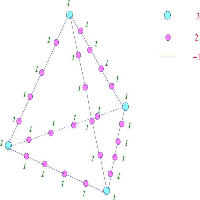
Figure 4: It is shown the typical the affine Berger graph from infinite series of the $CY_{3}$ graphs, corresponding to the ${\vec{k}}_{1}^{ext}=(1,0,0,0,0)$. One can see the labels which in KMA correspond to the Coxeter labels.

Figure 5: It is shown the typical affine Berger graph from infinite series of the $CY_{3}$ graphs corresponding to the ${\vec{k}}_{2}^{ext}=(0,0,0,1,1)$. One can see the labels, which in KMA correspond to the Coxeter labels.

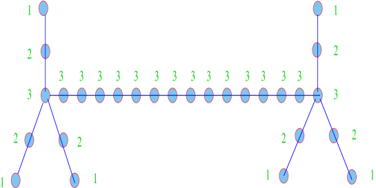
Figure 6: It is shown the typical affine Berger graph from infinite series of the $CY_{3}$ graphs corresponding to the ${\vec{k}}_{3}^{ext}=(0,0,1,1,1)$. One can see the labels, which in KMA correspond to the Coxeter labels.

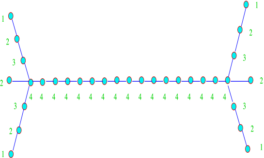
Figure 7: It is shown the typical affine Berger graph from infinite series of the $CY_{3}$ graphs, corresponding to the ${\vec{k}}_{3}^{ext}=(0,0,1,1,2)$. One can see the labels, which in KMA correspond to the Coxeter labels.

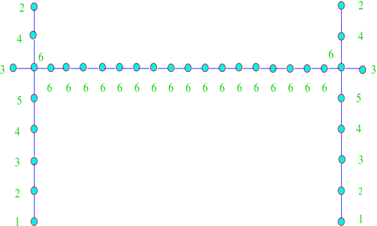
Figure 8: It is shown the typical affine Berger graph from infinite series of the $CY_{3}$ graphs, corresponding to the ${\vec{k}}_{3}^{ext}=(0,0,1,2,3)$. One can see the labels, which in KMA correspond to the Coxeter labels .

Let give more explanations for the first graph, what one can get from K3-fibre $CY_{3}$ space and which is defined by two extended vectors, $\vec{k}_{1}^{(ext)}=(1,0,0,0,0)$ and ${\vec{k}}_{4}^{(ext)}=(0,{\vec{k}}_{4})$. The second extended vector can be constructed from any of $95$ $K3$ weight vectors. The fibre structure of the $CY_{3}$, corresponding to the weight vector $\vec{k}_{5}=(1,k_{1},k_{2},k_{3},k_{4})$, is determined by $K3$ vector, ${\vec{k}}_{4}=(k_{1},k_{2},k_{3},k_{4})$. The left and right graphs of reflexive polyhedron are determined by extended vectors, $\vec{k}_{1}^{(ext)}=(1,0,0,0,0)$ and $\vec{k}_{4}^{(ext)}=(0,{\vec{k}}_{4})$, respectively. For simplicity one can consider the case when ${\vec{k}}_{4}=(1,1,1,1)[4]$. The graph corresponding to the extended vector $\vec{k}_{1}^{(ext)}=(1,0,0,0,0)$ will be a tetrahedron with 4-vertices and 6 edges. (If we take the ${\vec{k}}_{4}=(1,1,1,3)[6]$ the graph corresponding to the vector $\vec{k}_{1}^{(ext)}=(1,0,0,0,0)$ will be prisma.) For this graph the corresponding Berger matrix will be $28\times 28$, where $28$ equal to the number of all nodes, $4$ vertices and $24$ internal points. To reconstruct the Berger matrix let us take the following prescriptions to the four vertices (v) , internal (I) nodes and internal segments:

1. for the vertices will correspond the diagonal elements $\,{\mathbb B}_{i_{v}i_{v}}$, where
   $\,{\mathbb B}_{i_{v}i_{v}}\,=\,3$,        $i_{V}=1,2,3,4$;
   

2. for 24 internal nodes we take the diagonal elements
    ${\mathbb B}_{j_{I}j_{I}}\,=\,2$;
   

3. for each segment connected two nearest nodes will correspond the non-diagonal element of matrix ${\mathbb B}_{ij}$ with value
   ${\mathbb B}_{ij}\,=\,-1$;
   

4. if $i$ and $j$ are not joining by the same bond,
   $\,{\mathbb B}_{ij}\,=\,0$.
   

5. as one can see on the figure each node is labelled by number $1$,
   i.e. $a_{i}=1$, $i=1,\ldots,28$.
   

Then one can convince that for the matrix ${\mathbb B}$ of this graph all our conditions are satisfied. $Det{\mathbb B}=0$. All principal minors are positive definite. and

$$\sum_{j=1}^{28}{\mathbb B}_{ij}\cdot a_{j}={\vec{0}},$$ (19)

where the numbers $a_{i}=1$ are analog of the Coxeter labels for affine KMA, which can be get as the components of eigenvector with eigenvalue zero of affine matrix ${\mathbb B}$. The analog of Coxeter number for this graph or matrix is equal $h_{B}=28$. We will call ${\mathbb B}$ also by affine matrices similarly as it was in KMA. The very interesting pecularity of such graph that it is closed graph, like it was in affine KMA , where the graph $A_{r}^{(1)}$ was a loop, and all Coxeter labels were equal to $1$. Now we would like to say that all these conditions will be satisfied for any number of internal nodes. So, one can construct an infinite series of such graphs and matrices. One can also generalize this tetrahedron graph by prisma graph. For this case one should also prescribe to all vertices the diagonal elements equal to 3, and to all internal nodes the value $2$. Such graph one can find in the case when the second extended vector ${\vec{k}}^{ext}=(0,1,1,1,3)$. So, to study further this infinite series it is better to build a more simpler graph without internal nodes (see Figure 9) and compare with the graph $A_{2}^{(1)}$.

Figure 9: Berger affine graph $CYB_{3}^{(1)}$ . There are labels on the graph which correspond in KMA to Coxter labels.

Let consider the graphs and Cartan matrices for $A_{2}^{(1)}$ and for new $CYA_{3}^{(1)}graph$ ($(Det(A_{2}^{(1)})=0$ and $Det(CY3{\mathbb B}_{3}^{(1)})=0$).:

$${\mathbb A}_{2}^{(1)}=\left(\begin{array}[]{ccc}2&-1&-1\\ -1&2&-1\\ -1&-1&2\\ \end{array}\right)\qquad CY3{\mathbb B}_{3}^{(1)}=\left(\begin{array}[]{cccc}3&-1&-1&-1\\ -1&3&-1&-1\\ -1&-1&3&-1\\ -1&-1&-1&3\\ \end{array}\right)$$ (27)

Now we can consider more complicated graph $CY_{r}^{(1)}$ (see Fig. 4) where we put some internal Cartan nodes with $\alpha_{i}=2$. The number of such points can be arbitrary since the corresponding determinant will be equal zero. So this serie can be infinite like it was in Cartan-Lie case with $A_{r}^{(1)}$.

One can see an example of the generalized Cartan matrix for the case, like it was shown on the figure 4. We put into internal nodes with norm equal 2:

$$CY3{\mathbb B}_{5}^{(1)}=\left(\begin{array}[]{cccccc}3&-1&0&0&-1&-1\\ -1&2&-1&0&0&0\\ 0&-1&2&-1&0&0\\ 0&0&-1&3&-1&-1\\ -1&0&0&-1&3&-1\\ -1&0&0&-1&-1&3\\ \end{array}\right).$$ (34)

One can convince that the determinant of this matrix is also equal zero.

Such graphs and matrices can be easily generalized for $CY_{4}$, $CY_{5}$ and etc. For illustration on can give here the case of the matrix $CY4{\mathbb B}_{4}^{(1)}$ with $Det(CY4{\mathbb B}_{4}^{(1)})=0$ for the loop-graph in $CY_{4}$ polyhedron:

$$CY4{\mathbb B}_{4}^{(1)}=\left(\begin{array}[]{ccccc}4&-1&-1&-1&-1\\ -1&4&-1&-1&-1\\ -1&-1&4&-1&-1\\ -1&-1&-1&4&-1\\ -1&-1&-1&-1&4\\ \end{array}\right)$$ (40)

Similarly, one can reconstruct the Berger matrices for the graphs indicated on the Figures 5,6,7,8. To satisfy to our conditions one should prescribe to the vertex-nodes the value of the corresponding diagonal elements 3. To all other nodes one should prescribe the value 2. In all graphs the number of internal nodes can be any, so one can get an infinite numbr of such graphs or Berger matrices. For example,consider the Berger matrix for the graph on the Fig.6.

$${\mathbb B}(EG3)=$$

$$\left(\begin{array}[]{ccccccc|ccc|ccccccc}2&-1&0&0&0&0&0&0&0&0&0&0&0&0&0&0&0\\ -1&2&0&0&0&0&-1&0&0&0&0&0&0&0&0&0&0\\ 0&0&2&-1&0&0&0&0&0&0&0&0&0&0&0&0&0\\ 0&0&-1&2&0&0&-1&0&0&0&0&0&0&0&0&0&0\\ 0&0&0&0&2&-1&0&0&0&0&0&0&0&0&0&0&0\\ 0&0&0&0&-1&2&-1&0&0&0&0&0&0&0&0&0&0\\ 0&-1&0&-1&0&-1&3&-1&0&0&0&0&0&0&0&0&0\\ \hline\cr 0&0&0&0&0&0&-1&2&-1&0&0&0&0&0&0&0&0\\ 0&0&0&0&0&0&0&-1&2&-1&0&0&0&0&0&0&0\\ 0&0&0&0&0&0&0&0&-1&2&-1&0&0&0&0&0&0\\ \hline\cr 0&0&0&0&0&0&0&0&0&-1&3&-1&0&-1&0&-1&0\\ 0&0&0&0&0&0&0&0&0&0&-1&2&-1&0&0&0&0\\ 0&0&0&0&0&0&0&0&0&0&0&-1&2&0&0&0&0\\ 0&0&0&0&0&0&0&0&0&0&-1&0&0&2&-1&0&0\\ 0&0&0&0&0&0&0&0&0&0&0&0&0&-1&2&0&0\\ 0&0&0&0&0&0&0&0&0&0&-1&0&0&0&0&2&-1\\ 0&0&0&0&0&0&0&0&0&0&0&0&0&0&0&-1&2\\ \end{array}\right)$$ (58)

One can convince that the determinant of this matrix is equal zero. For illustration we put into internal line only two nodes, but the determinant will be equal zero for any number of the nodes in internal line. As we already said this serie is infinite.

So in all 4-cases cases the Berger matrices are degenerated and all principal minors are positive definite. Also, the labels, which we can find from matrices will be equal to those what we can reconstruct directly from polyhedra, and which we indicated on the all graphs. If one takes out one zero node with label 1, he will get the non-affine Berger graphs. The determinants of non-affine Berger matrices for these three non-affine graphs 6,7,8, are equal $9^{2}$, $8^{2}$, $6^{2}$, respectively and don’t depend on the number internal nodes.

These graphs and their analyse can be also considered in $CY_{d}$ with $d\geq 4$. For example, one can see on the next Figure 10, the Berger graph which we found from $CY_{6}$. On the Figures 11,12 and 13 we give the Berger graphs from $CY_{4}$. According to these graphs one can easily to reconstruct the Berger matrices. For this one should prescribe for the vertex-nodes in $CY_{6}$ and $CY_{4}$ cases, the value 6 and 4, respectively.

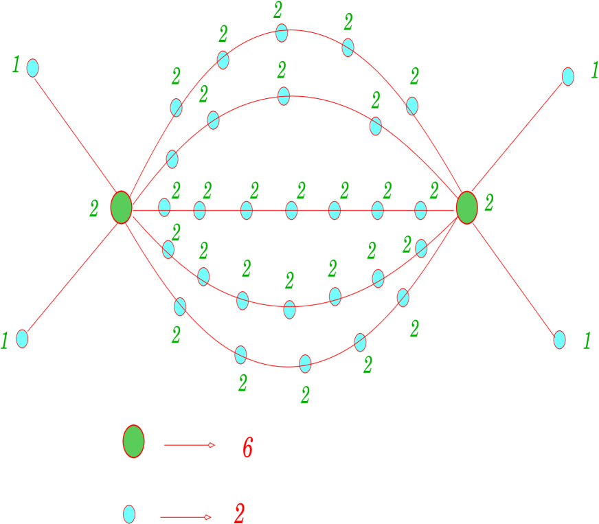
Figure 10: Berger graph in $CY_{6}$ polyhedron, corresponding to ${\vec{k}}_{8}(1,0,0,0,0,0,0,1)+...$. One can see the labels, which correspond in KMA to the Coxeter labels

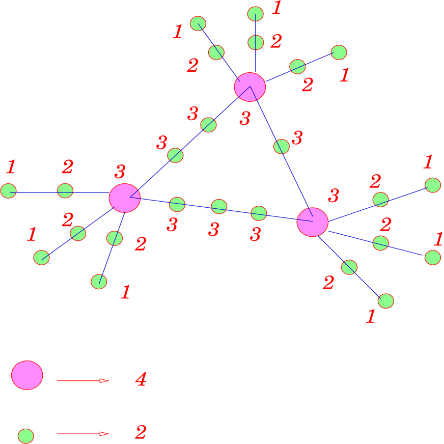
Figure 11: The Berger affine graph in $CY_{4}$ polyhedron, corresponding to ${\vec{k}}_{6}=(1,0,0,0,1,1)+...$. There are indicated the labels which correspond in KMA to the Coxeter labels

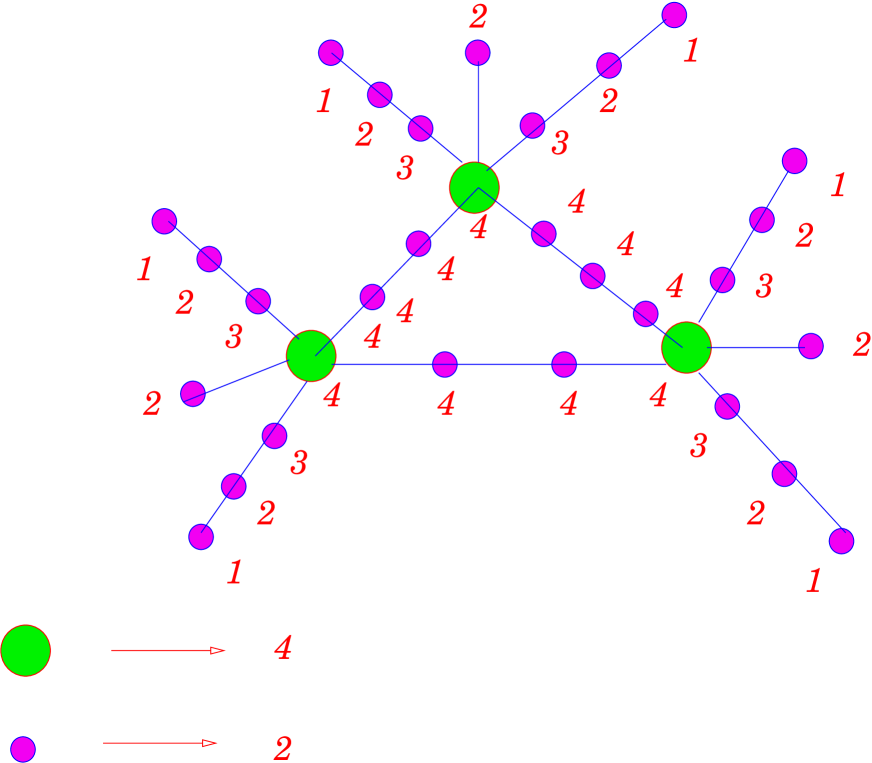
Figure 12: Berger affine $CY_{4}$ graph, corresponding to the RWV ${\vec{k}}_{6}=(1,0,0,0,1,2)+...$. One can see the labels which correspond in KMA to the Coxeter labels.

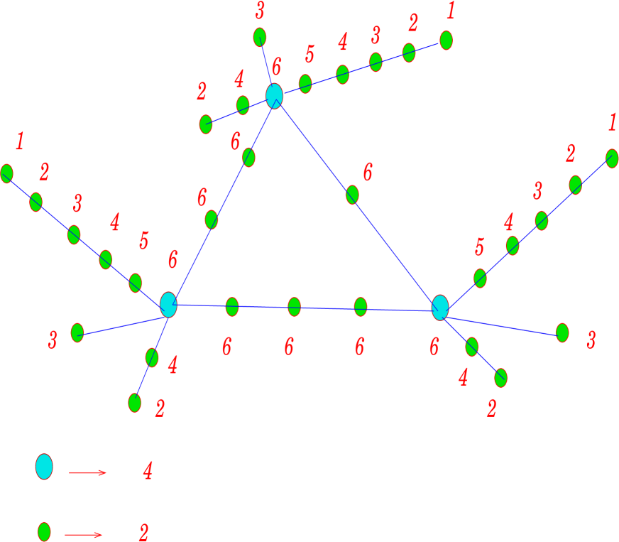
Figure 13: Berger affine graph in $CY_{4}$ polyhedron, corresponding to ${\vec{k}}_{6}=(1,0,0,0,2,3)+...$. One can see the labels which correspond in KMA to the Coxeter labels.

For example, one can consider the graph based on the vector ${\vec{k}}_{n}=(1,\ldots,1)[n]$, where $n=3,4,5,...$.

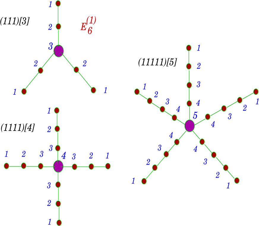
Figure 14: The infinite series of Berger Flower graphs, corresponding to the vectors ${\vec{k}}_{n}=(1,\ldots,1)[n]$. There are indicated the labels corresponding to the Coxeter labels.

These graphs have much more different structure comparing to the affine Dynkin graphs. There is a vertex-node with 4(5)-lines. We call this graph as generalized $AENV4^{(1)}$ ($AENV5^{(1)}$) graph. We suppose that these graphs produce an infinite series of $CY_{2,3,4,...}E_{6}^{(1)}$ symmetries. The first term in this infinite series starts from very-well-known $E_{6}^{(1)}$ symmetry. The determinant of generalized Cartan matrix for all cases is equal zero. Here we give an example of such matrix for the graph in $CY_{3}$ case:

$$Det(AENV4^{1}) =$$ (73)

$$\left(\begin{array}[]{ccc|ccc|ccc|ccc|c}2&-1&0&0&0&0&0&0&0&0&0&0&0\\ -1&2&-1&0&0&0&0&0&0&0&0&0&0\\ 0&-1&2&0&0&0&0&0&0&0&0&0&-1\\ \hline\cr 0&0&0&2&-1&0&0&0&0&0&0&0&0\\ 0&0&0&-1&2&-1&0&0&0&0&0&0&0\\ 0&0&0&0&-1&2&0&0&0&0&0&0&-1\\ \hline\cr 0&0&0&0&0&0&2&-1&0&0&0&0&0\\ 0&0&0&0&0&0&-1&2&-1&0&0&0&0\\ 0&0&0&0&0&0&0&-1&2&0&0&0&-1\\ \hline\cr 0&0&0&0&0&0&0&0&0&2&-1&0&0\\ 0&0&0&0&0&0&0&0&0&-1&2&-1&0\\ 0&0&0&0&0&0&0&0&0&0&-1&2&-1\\ \hline\cr 0&0&-1&0&0&-1&0&0&-1&0&0&-1&3\\ \end{array}\right)$$

Note, that the determinant is equal zero. If we remove the zero node ( label =1), the $Det(ENV4)=4^{2}$. In general case for $CY_{d}$, $d+2=n$, which corresponded to the RWV ${\vec{k}}_{n}=(1,\ldots,1)[n]$, the determinant of the corresponding non-affine matrix is equal $n^{n-2}$ ( $n\geq 3$).

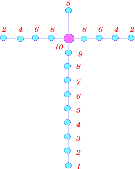
Figure 15: Berger affine Cross graph in $CY_{3}$ polyhedron ${\vec{k}}_{4}=(1,1,2,2,5)[11]=(1,0,0,0,0)+(0,1,2,2,5)$ with (1,2,2,5)- intersection. One can see the labels which correspond to the Coxeter labels.

4 Discussion

The interest to look for new algebras beyond Lie algebras started from the $SU(2)$- conformal theories ( see for example [12, 16]). But it seems that the geometrical way is a more natural way to do this. Let remind that to prove mirror symmetry of Calabi-Yau spaces, the greatest progress was reached with using the technics of Newton reflexive polyhedra in [6].

We considered here examples of some new graphs from $CY_{d}$ ($d\geq 3$) reflexive polyhedra, which can be in one-to-one correspondence to the new algebras, like it was in $CY_{2}\equiv K3$ case, where one can find the Cartan-Lie algebra. In UCYA these new graphs are closely related to the (1+1+3+95) reflexive weight-vectors, giving us all fibre-structure of $CY_{3}$. We illustrated on some graphs a possible link to the new algebras only for some simply-laced examples ( the case of symmetric Berger matrices) from 100 possible general cases. What it is very remarkable is that some of these graphs naturally can be extended into infinite series. It is very well known that Dynkin diagram one-to-one defines a Cartan-Lie algebra. We transported some of the properties of Cartan matrices for CLA and KMA to look for new graphs. We have formulated some new properties for the affine Berger matrices. Cheking by this way the graphs in $CY_{d}$ we have got some information for new possible algebras. In new graphs for some special nodes, we only changed the diagonal elements in Berger matrices, i.e. for vertex-nodes we took a norm equal to 3. This number was chosen by us taking in minds two points. One is connected to the Euler number of $CP^{2}$ space, which could be use for resolution of some singularities in $CY_{3}$ space. We already knew, that for resolution of quotient singularities in K3 case one should use the $CP^{1}$ with Euler number 2. The second point is going from the cubic matrix approach [24], in which the $S_{3}$ group is naturally created. So, the new node-vertices with norm 3 could be connected with new universal algebra, which apart from the usual binary Lie algebra operations contain the elements of ternary algebra. For our goal we should find a way for unify description of binary and ternary composition laws, since we propose that these new graphs following from $CY_{3}$,($CY_{4},...$) polyhedra can lead us to the universal algebras, having at two (three,…) arity operations, binary ( ternary,….). It is also interesting to note that these graphs correspond to the affine algebras. In nearest future publications we will plan to continue an analysis of the others graphs from 100 reflexive weight vectors.

5 Akcnowledgements

I would like to give a lot of thanks to E. Alvarez, L. Alvarez-Gaume, F.Anselmo, P. Auranche, P. Chankowski, R. Coquereaux, N. Costa, L. Fellin, M.P. Garcia del Moral, B. Gavela, C. Gomez, G. Harigel, J.Ellis, A. Erikalov, V.Kim, N. Koulberg, A. Kulikov, P. Kulish, A. Liparteliani, L.Lipatov, A. Masiero, C. Mu$\tilde{n}$oz, A. Sabio Vera, J. Sanchez Solano, P.Sorba, E. Torrente-Lujan, A. Uranga, G. Valente, G. Volkova and A. Zichichi for valuable discussions, for important help and nice support.

6 Bibliography

References

-
[1]
F. Anselmo, J. Ellis, D. V. Nanopoulos and G. G. Volkov,
Towards a Algebraic Classification of Calabi-Yau Manifolds
I: Study of K3 Spaces,
Phys.Part.Nucl. 32 (2001) 318-375;
Fiz.Elem.Chast.Atom.Yadra 32 (2001) 605-698.
- [2] F. Anselmo, J. Ellis, D. V. Nanopoulos and G. G. Volkov, Results from an Algebraic Classification of Calabi-Yau Manifolds, Phys.Lett. B499 (2001) 187-199.
-
[3]
F. Anselmo, J. Ellis, D. V. Nanopoulos and G. G. Volkov,
Universal Calabi-Yau Algebra: Towards an Unification of
Complex Geometry, Int. J. Mod. Phys. (2003),
hep-th/0207188.
-
[4]
F. Anselmo, J. Ellis, D. V. Nanopoulos and G. G. Volkov,
Universal Calabi-Yau algebra: Classification and enumeration of
Fibrations , Mod. Phys.Lett.A v.18, No.10 (2003) pp.699-710,
hep-th/0212272.
-
[5]
O.Brwald, R. W. Gebert and H. Nicolai,
On the Imaginary Simple Roots of the Borcherds Algebra
. preprint hep-th/9705144.
-
[6]
V. Batyrev, Dual Polyhedra and Mirror Symmetry for Calabi-Yau
Hypersurfaces in Toric Varieties, J. Algebraic Geom. 3 (1994)
493;
-
[7]
M. Berger, Sur les groupesd’holonomie des varietes a connexion affine
et des varietes riemanniennes, Bull.Soc.Math.France 83 (19955),279-330.)
-
[8]
M. Bershadsky, K. Intriligator, S. Kachru, D.R. Morrison, V. Sadov,
and C. Vafa, Geometric Singularities and Enhanced Gauge Symmetries,
Nucl. Phys. B481 (1996) 215.
-
[9]
S. Burris and H.P. Sankappnavar,
A Course in Universal Algebra, The Millennium Edition, 2001.
-
[10]
P. Candelas and A. Font, Duality Between the Webs of Heterotic and
Type II Vacua, Nucl. Phys. B511 (1998) 295;
-
[11]
P. Candelas, G. Horowitz, A. Strominger and E. Witten, Nucl. Phys.
B258 (1985) 46;
-
[12]
A. Capelli, C. Itzykson and J.-B. Zuber,
The ADE classification of minimal and
conformal invariant theories,
Commun. Math. Phys. 184 (1987), 1-26, MR 89b, 81178.
-
[13]
P. Candelas, E. Perevalov and G. Rajesh,
Toric Geometry and Enhanced Gauge Symmetry of
F-Theory/Heterotic Vacua, Nucl. Phys. B507 (1997) 445;
P. Candelas, E. Perevalov and G. Rajesh, Matter from Toric Geometry, Nucl. Phys. B519 (1998) 225;
-
[14]
R. Carter, G.Segal, I. Macdonald,
Lectures on Lie Groups and Lie algebras,
London Mathematical Society 32 (1995).
-
[15]
P. Du Val, Homographies, Quaternions and Rotations (Clarendon Press,
Oxford 1964);
-
[16]
P.Di Francesco and J.-B. Zuber,
SU(N) Lattice integrable models associated
with graphs, N.P.B 338 (1990), no 3, 602-646.
- [17] L. Frappat, A. Sciarrino, P. Sorba, Dictionary on Lie Algebras and Superalgebras Academic Press (2000).
-
[18]
J.Fuchs,
Affine Lie Algebras and Quantum Groups
Cambridge, University press, (1992).
-
[19]
C. Gómez and R. Hernández,
Fields, Strings and Branes,
IFT-UAM-CSIC-97-4, hep-th/9711102.
-
[20]
P.Goddard, and D.Olive,
Int.J.Mod.Phys. A1 (1986) 1.
- [21] B.R. Greene, String Theory on Calabi-Yau Manifolds, CU-TP-812, hep-th/9702155.
-
[22]
M.B. Green, J.H. Schwartz, E. Witten,
Superstring Theory, Vol. I, II, Cambridge University Press,
(1987).
-
[23]
E.A. de Kerf, G.G.A. Buerle, A.P.E. Kroode,
Lie algebrasFinite and infinite dimensional Lie algebras
and appliations in physics Part2 North-Holland (1997).
-
[24]
R. Kerner,
The cubic chessboard
math-ph/0004031, (2000).
-
[25]
S. Katz and C. Vafa Geometric Engineering of Quantum Field
Theories, Nucl. Phys. B497 (1997) 196;
S. Katz and C. Vafa, Matter from Geometry, Nucl. Phys. B497 (1997) 146;
-
[26]
K.Kodaira, On compact analytic surfaces.II
Annals og Mathematics, v77), (1963), 563-626.
-
[27]
J.L.Loday, La renaissance des operads,
Expose 792 Seminaire Bourbaki,
Asterique (1994/95).
-
[28]
A.A. Maslikov, S.M. Sergeev, G.G. Volkov,
Phys. Lett. B328. (1994), 319; Phys. Rev. D50. (1994), 7740;
Int. J.Mod. Phys. A11., (1996) 1117;
S.M. Sergeev and G.G. Volkov, preprint DFPD/TH/51, 1992; Physics of Atomic Nuclei v.57, (1994) 168.
-
[29]
G.Slodowy, A new ADE classification , Bayreuth. Math. Schr. (1990),
no. 33, 395-424.
-
[30]
B.G. Wyborne, Classical Groups for Physicists,
A Wyley-Interscience Publication (1974).