Quark-antiquark pair production in space-time dependent fields

Abstract

Fermion-antifermion pair-production in the presence of classical fields is described based on the retarded and advanced fermion propagators. They are obtained by solving the equation of motion for the Dirac Green’s functions with the respective boundary conditions to all orders in the field. Subsequently, various approximation schemes fit for different field configurations are explained. This includes longitudinally boost-invariant forms. Those occur frequently in the description of ultrarelativistic heavy-ion collisions in the semiclassical limit. As a next step, the gauge invariance of the expression for the expectation value of the number of produced fermion-antifermion pairs as a functional of said propagators is investigated in detail. Finally, the calculations are carried out for a longitudinally boost-invariant model-field, taking care of the last issue, especially.

I Introduction

In field the inclusive spectra of fermion-antifermion pairs produced by vacuum polarisation in the presence of time-dependent classical fields were studied based on the exact retarded propagator. Here the generalisation to arbitrarily space-time dependent fields is presented. Processes of this kind in quantum electrodynamics (QED) baltz ; qed as well as in quantum chromodynamics (QCD) qcd are of importance for the physics of the early universe cornwall and strong laser fields laser as well as of ultrarelativistic heavy-ion collisions and the quark-gluon plasma (QGP) kinetic . The strong classical fields are the common feature of these phenomena, while the detailed characteristics of the field configurations differ. Although this paper ultimately concentrates on ultrarelativistic heavy-ion collisions, various other kinematical regimes are treated as well (see section II).

A lot of effort is made to study the QGP’s production and equilibration qm in nuclear collision experiments at the Relativistic Heavy-Ion Collider (RHIC) and the Large Hadron Collider (LHC), currently under construction. It is a widely used hypothesis that the initial state in heavy-ion collisions is dominated by gluons which on account of their large occupation number can be treated as a classical background field. The larger the occupation number $N_{k}$ of the bosonic sector at a given momentum $k$ of a physical system, i.e., the better $N_{k}\gg 1$ is satisfied, the more accurately it can be described by a classical field. In a heavy-ion collision at RHIC with $\sqrt{s}=130$GeV the initial occupation number for gluons at their average transverse momentum $|\vec{k}_{T}|\approx 1$GeV in the center of the collision is approximately equal to 1.5 mueller . Even if this number is not much larger than unity, the classical field as the expectation value of the gauge field still represents the parametrically leading contribution. At this scale, keeping only classical bosons is a first approximation but quantum fluctuations have to be investigated subsequently.

One concrete model based on this idea is due to McLerran and Venugopalan jimwlk . In that approach, classically interacting colour-charge distributions on the two branches of the light-cone represent the two colliding nuclei. However, there, it turns out that quantum corrections become important due to kinematical factors. Nevertheless, this approach can be extended farther by including quantum evolution in the distribution of the classically interacting charges. This extension leads to the so-called JIMWLK equation jimwlk .

Be that as it may, the magnitude of the high occupation-number bosonic fields is such that multiple couplings to the classical field, i.e., higher powers of the product of the coupling constant $g$ and the gauge field strength $A$, are not parametrically suppressed. In the absence of other scales they have to be addressed to all orders. Under the prerequisite of weak coupling the leading quantum processes concern terms in the classical action of second order in the quantum fields (fermions, antifermions, and bosonic quantum-fluctuations). These terms’ coefficients give the inverse of the respective two-point Green’s functions. Their inversion for selected boundary conditions yields the propagators of the corresponding particles to all orders in the classical field. As an alternative, the full propagator can also be derived by resumming all terms of the perturbative series or by adding up a complete set of wave-function solutions of the equations of motion.

Since exact solutions are not easily obtainable some general approximation schemes have been devised. Expansion of the propagators in powers of the field leads to the perturbative series which is based on the free Green’s functions. Neglecting the spatial part of the field and the derivatives yields what is called the static approximation. Other approaches for the fermionic propagator can be found in gromes .

In this paper the phenomenon of particle production is to be investigated based on the propagator in the classical field. The required correlator is obtained by direct solution of the equation of motion. In QED as well as QCD the direct production of fermion-antifermion pairs occurs (electron-positron and quark-antiquark, respectively). Caused by the non-linearity of the gauge-field tensor in QCD also pairs of gluonic quantum fluctuations are created. There, in strong fields the two types of reactions are equally parametrically favoured.

In a given situation the bosonic sector could be covered sufficiently well by the concept of a classical field and the hard sector be accessible perturbatively ddd . However, due to Pauli’s principle, it exists no such concept for the fermions. Perturbative investigations can only describe the hard not the soft part. Hence, this paper deals predominantly with the description of fermions and antifermions.

In constant fields, the Schwinger mechanism schwinger gives the exact answer to the problem of particle production. Frequently, its application is extended to slowly varying fields and/or low-energy particles. It, like most of the other schemes, is based on assumptions on time and/or energy scales of the situation under investigation. However, if such scales are to be obtained by means of a calculation it is likely that they are strongly biased by the choice of the approximation comparison .

Finally, it is necessary to decide whether expectation values are to be obtained in the framework of the in-in-formalism of quantum field theory – i.e., based on the advanced and retarded propagator and their relatives – or probabilities within that of the in-out-formalism – i.e., starting out from the Feynman propagator – field ; baltz . As the average number of produced pairs is the more natural observable as compared to the probability to produce exactly a given number $n$ of pairs in a particular event, the first possibility will be pursued here.

Therefore, section II presents the solution of the equation of motion for the retarded Dirac propagator to all orders in the field. Respective subsections include details on a generalised translation operator that occurs during the derivation as well as on the propagator in a large variety of expansion schemes and classes of field configurations. This includes longitudinally boost-invariant field configurations which can be of importance in the description of the initial phase of an ultrarelativistic heavy-ion collisions. Section III contains the application of the results of section II to the problem of particle production in general. This includes a thorough discussion of the gauge invariance of the result. In a subsection the formulae are evaluated for a longitudinally boost-invariant model-field. In the last chapter the contents of the paper are summarised.

Throughout the paper the metric tensor is given by: $g^{\mu\nu}={\rm diag}(1,-1,-1,-1)$, angular momenta are measured in units of $\hbar$, and velocities in fractions of the speed of light $c$. From hereon, the coupling constant is included in the definition of the classical field: $gA^{\mu}_{old}=A^{\mu}_{new}$. The convention for Fourier transformations of one-point functions is:

$$f(x)=\int\frac{d^{4}k}{(2\pi)^{4}}e^{-ik\cdot x}f(k),$$ (1)

that for two-point functions:

$$f(x,y)=\int\frac{d^{4}p}{(2\pi)^{4}}\frac{d^{4}q}{(2\pi)^{4}}e^{-iq\cdot x}e^{+ip\cdot y}f(q,p).$$ (2)

II The retarded fermion-propagator

If the fermionic propagators for the in-in-formalism are known to all orders in the classical field the generating functional of the Green’s functions without radiative corrections can be written as:

$$Z[{\bf\bar{\eta}},{\bf\eta}]=\exp\left\{i\int d^{4}xd^{4}y~{}\bar{\eta}_{\sigma_{1}}(x)G_{\sigma_{1}\sigma_{2}}(x,y)\eta_{\sigma_{2}}(y)\right\},$$ (3)

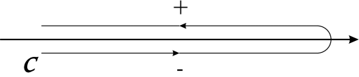
Figure 1: Contour of integration in the complex time-plane for the Schwinger-Keldysch formalism

with implicit sums over $\sigma_{1,2}\in\{+,-\}$. These indices refer to the sign of the imaginary part of the time component of $x$ or $y$ respectively, taken along the contour in the complex time-plane shown in figure 1 sk . Hence, the components of the matrix propagator $G_{\sigma_{1}\sigma_{2}}$ correspond to:

$$G_{++}(x,y) = +\left<0_{in}\right|T\bar{\psi}(y)\psi(x)\left|0_{in}\right>~{}$$

$$G_{--}(x,y) = +\left<0_{in}\right|T^{-1}\bar{\psi}(y)\psi(x)\left|0_{in}\right>~{}$$

$$G_{+-}(x,y) = +\left<0_{in}\right|\bar{\psi}(y)\psi(x)\left|0_{in}\right>~{}$$

$$G_{-+}(x,y) = -\left<0_{in}\right|\psi(x)\bar{\psi}(y)\left|0_{in}\right>,$$ (4)

where $T^{-1}$ stands for reverse time-ordering. The components of the matrix propagator $G_{\sigma_{1}\sigma_{2}}$ can be linked to the advanced (A), retarded (R), and on-shell (S) propagator by:

$$2G_{\sigma_{1}\sigma_{2}}=G_{S}+\sigma_{1}G_{A}+\sigma_{2}G_{R}.$$ (5)

What is called the on-shell propagator is a solution of the homogeneous Dirac equation. The advanced and the retarded propagator solve the equation of motion of the Dirac Green’s functions:

$$\left[i\gamma\cdot\partial(x)+\gamma\cdot A(x)-m\right]G(x,y)=\delta^{(4)}(x-y).$$ (6)

Let us consider homogeneous solutions $G_{H}(x,y)$ of Dirac’s equation, i.e., with the $\delta$-distribution replaced by zero using a product as an ansatz:

$$G_{H}(x,y)=U(x_{0}-y_{0})\hat{G}_{H}(x,y).$$ (7)

The differential equation obeyed by the functional $U(x_{0}-y_{0})$ is to be the following:

$$[i\gamma^{0}\partial_{0}(x)U(x_{0}-y_{0})]\hat{G}_{H}(x,y)+i\gamma^{j}\partial_{j}(x)U(x_{0}-y_{0})\hat{G}_{H}(x,y)=0,$$ (8)

with a summation over $j\in\{1,2,3\}$ and where the solution for the boundary condition $U(0)=1$ is given by:

$$U(x_{0}-y_{0})=\exp[-(x_{0}-y_{0})\gamma^{0}\gamma^{j}\partial_{j}(x)].$$ (9)

This object corresponds to a generalised translation operator taking care of the relativity of events, as shall be explained in section II.1. With equation (8) and after subsequent multiplication by $-iU(y_{0}-x_{0})\gamma^{0}$ from the left, the remaining differential equation for the second factor $\hat{G}_{H}(x,y)$ of the homogeneous solution reads:

$$\partial_{0}(x)\hat{G}_{H}(x,y)-iU(y_{0}-x_{0})\gamma^{0}[\gamma\cdot A(x)-m]U(x_{0}-y_{0})\hat{G}_{H}(x,y)=0,$$ (10)

where the inverse of the generalised translation operator (9) is given by inverting the sign of its argument: $U^{-1}(x_{0}-y_{0})=U(y_{0}-x_{0})$. For the boundary condition $G_{H}(x_{0}=y_{0},\vec{x},\vec{y})=1$ the last differential equation is solved by a path-ordered exponential field :

$$\hat{G}_{H}(x,y)={\cal P}\exp\left\{i\int_{y_{0}}^{x_{0}}d\xi_{0}U(y_{0}-\xi_{0})\gamma^{0}\left[\gamma\cdot A(\xi_{0},\vec{x})-m\right]U(\xi_{0}-y_{0})\right\}.$$ (11)

Other boundary conditions would only lead to additional factors to the right of the above solution which would not result in independent expressions, because a homogeneous differential equation is investigated here. The homogeneous solution $G_{H}(x,y)$ can be reassembled from equations (9) and (11) according to equation (7). The boundary condition for vanishing time difference $x_{0}-y_{0}$ for all Dirac Green’s functions is given by $[\lim_{x_{0}\rightarrow y_{0}+0}-\lim_{x_{0}\rightarrow y_{0}-0}]G(x,y)=-i\gamma^{0}\delta^{(3)}(\vec{x}-\vec{y})$. Additionally, the retarded propagator $G_{R}(x,y)$ is required to vanish for negative time differences: $G_{R}(x,y)=0~{}{\rm if}~{}x_{0}<y_{0}$; the advanced for positive: $G_{A}(x,y)=0~{}{\rm if}~{}x_{0}>y_{0}$. By virtue of the boundary condition chosen for equation (11) the retarded propagator can be expressed as:

$$iG_{R}(x,y)\gamma^{0}=+G_{H}(x,y)\delta^{(3)}(\vec{x}-\vec{y})\theta(x_{0}-y_{0}),$$ (12)

the advanced as:

$$iG_{A}(x,y)\gamma^{0}=-G_{H}(x,y)\delta^{(3)}(\vec{x}-\vec{y})\theta(y_{0}-x_{0}).$$ (13)

With the help of the general resummation formula derived in field :

$${\cal P}\exp\left\{\int^{x_{0}}_{y_{0}}d\xi_{0}[B(\xi_{0})+C(\xi_{0})]\right\}=~{}$$ (14)

$$= {\cal P}\exp\left\{\int^{x_{0}}_{y_{0}}d\xi_{0}B(\xi_{0})\right\}\times~{}$$

$$\times{\cal P}\exp\left[\int^{x_{0}}_{y_{0}}d\xi_{0}{\cal P}\exp\left\{\int_{\xi_{0}}^{y_{0}}dz_{0}B(z_{0})\right\}C(\xi_{0}){\cal P}\exp\left\{\int^{\xi_{0}}_{y_{0}}dz_{0}B(z_{0})\right\}\right]=~{}$$

$$= {\cal P}\exp\left[\int^{x_{0}}_{y_{0}}d\xi_{0}{\cal P}\exp\left\{\int_{\xi_{0}}^{x_{0}}dz_{0}B(z_{0})\right\}C(\xi_{0}){\cal P}\exp\left\{\int^{\xi_{0}}_{x_{0}}dz_{0}B(z_{0})\right\}\right]\times~{}$$

$$\times{\cal P}\exp\left\{\int^{x_{0}}_{y_{0}}d\xi_{0}B(\xi_{0})\right\},$$

which is based on the group property valid for path-ordered exponentials:

$${\cal P}\exp\left\{\int_{y_{0}}^{x_{0}}d\xi_{0}B(\xi_{0})\right\}={\cal P}\exp\left\{\int_{z_{0}}^{x_{0}}d\xi_{0}B(\xi_{0})\right\}\times{\cal P}\exp\left\{\int_{y_{0}}^{z_{0}}d\xi_{0}B(\xi_{0})\right\},$$ (15)

the generalised translation operators can be included into the principal path-ordered exponential:

$$iG_{R}(x,y)\gamma^{0}=\int\frac{d^{3}k}{(2\pi)^{3}}e^{+i\vec{k}\cdot(\vec{x}-\vec{y})}G_{H}(x,y,\vec{k})\theta(x_{0}-y_{0})=~{}$$

$$= \int\frac{d^{3}k}{(2\pi)^{3}}e^{+i\vec{k}\cdot(\vec{x}-\vec{y})}{\cal P}\exp\left\{i\int_{y_{0}}^{x_{0}}d\xi_{0}\gamma^{0}\left[i\gamma^{j}\partial_{j}(x)+\gamma^{j}k_{j}+\gamma\cdot A(\xi_{0},\vec{x})-m\right]\right\}\theta(x_{0}-y_{0})~{}$$

Here, the $\delta$-distribution has been replaced by its Fourier representation. The path-ordered exponential in equation (II) corresponds to a special mixed representation of the homogeneous solution $G_{H}$. Only the spatial relative coordinates have been Fourier transformed to the momentum space. The absolute coordinate is kept in the coordinate space. This becomes clearer by noticing that, because of the $\delta$-distribution introduced by the boundary conditions, $\vec{x}$ in the path-ordered exponential can always be replaced by $\vec{y}$ and also by $(\vec{x}+\vec{y})/2$. Due to its mixed boundary conditions for positive and negative energy solutions, the Feynman propagator cannot be expressed in a similar way. Henceforth, unless otherwise stated, $G(x,y)$ also without the index _R shall stand for the retarded propagator.

II.1 Generalised translation operator

In one spatial dimension, the object in equation (9) is linked to common translation operators $\exp\{-t\partial_{3}\}$ through:

$$U_{3}(+t)=\exp\{-t\gamma^{0}\gamma^{3}\partial_{3}\}=\rho^{+}e^{-t\partial_{3}}+\rho^{-}e^{+t\partial_{3}},$$ (17)

where $2\rho^{\pm}=1\pm\gamma^{0}\gamma^{3}$ are two projectors, whence $(\rho^{\pm})^{2}=\rho^{\pm}$ and $\rho^{\pm}\rho^{\mp}=0$. In three dimensions, the operator (9) transforms a $\delta$-distribution localised at $\vec{x}=\vec{y}$ into:

$$\exp\{-t\gamma^{0}\gamma^{j}\partial_{j}(x)\}\delta^{(3)}(\vec{x}-\vec{y})=\frac{1}{4\pi}\left[\partial_{t}+\gamma^{0}\gamma^{j}\partial_{j}(x)\right]\frac{\delta(|\vec{x}-\vec{y}|-t)-\delta(|\vec{x}-\vec{y}|+t)}{|\vec{x}-\vec{y}|}.$$ (18)

The effect on any other function can be investigated by a convolution of it with the previous equation. The corresponding integral has only support in the distance $t$ from the point $\vec{x}$ along the light-cone, i.e., on a sphere of radius $t$. After making use of the one-dimensional $\delta$-distributions there remain two angular integrations $d\Phi$ which represent an average of the equidistant shifts over all directions $\hat{\vec{z}\hskip 1.42262pt}(\Phi)$ ($|{\hat{\vec{z}\hskip 1.42262pt}}|=1$):

$$\exp\{-t\gamma^{0}\gamma^{j}\partial_{j}(x)\}f(\vec{x})=\frac{1}{2}\left[\partial_{t}+\gamma^{0}\gamma^{j}\partial_{j}(x)\right]\int\frac{d\Phi}{4\pi}t[f(\vec{x}+\hat{\vec{z}}t)+f(\vec{x}-\hat{\vec{z}}t)],$$ (19)

where $\vec{x}$ is the center of the coordinate system. The differential operator on the right-hand side of the last equation serves to assign the correct element of the Clifford algebra to every contribution of the integral.

II.2 Expansion schemes

In this section, various expansion schemes for the retarded propagator are presented. This shall serve to establish the connection to the results in the purely time-dependent case field . Like there they are also to help to expose the characteristics of the full expression.

II.2.1 Weak-field expansion

In order to obtain the weak-field expansion, the general resummation formula (14) can be used to transform the path-ordered exponential in equation (II) with the choice $C(\xi_{0})=i\gamma^{0}\gamma\cdot A(\xi_{0})$. After expanding the result in powers of the gauge field, $G_{H}=\sum_{n}G_{H}^{(n)}$, and Fourier transformation of the vector potential into a mixed representation one finds up to the second order:

$$G_{H}^{(0)}(x,y,\vec{k})=\exp\{i\gamma^{0}[\gamma^{j}k_{j}-m](x_{0}-y_{0})\}$$ (20)

$$G^{(1)}_{H}(x,y,\vec{k}) = i\int_{y_{0}}^{x_{0}}d\xi_{0}\int\frac{d^{3}\kappa}{(2\pi)^{3}}e^{+i\vec{\kappa}\cdot\vec{x}}\times~{}$$ (21)

$$\times\exp\{i\gamma^{0}[\gamma^{j}(k_{j}+\kappa_{j})-m](x_{0}-\xi_{0})\}i\gamma^{0}\gamma\cdot A(\xi_{0},\vec{\kappa})\times~{}$$

$$\times\exp\{i\gamma^{0}[\gamma^{j}k_{j}-m](\xi_{0}-y_{0})\},$$

$$G^{(2)}_{H}(x,y,\vec{k}) = i\int_{y_{0}}^{x_{0}}d\xi_{0}i\int_{y_{0}}^{\xi_{0}}d\eta_{0}\int\frac{d^{3}\kappa}{(2\pi)^{3}}\frac{d^{3}\lambda}{(2\pi)^{3}}e^{+i(\vec{\kappa}+\vec{\lambda})\cdot\vec{x}}\times~{}$$ (22)

$$\times\exp\{i\gamma^{0}[\gamma^{j}(k_{j}+\kappa_{j}+\lambda_{j})-m](x_{0}-\xi_{0})\}i\gamma^{0}\gamma\cdot A(\xi_{0},\vec{\kappa})\times~{}$$

$$\times\exp\{i\gamma^{0}[\gamma^{j}(k_{j}+\lambda_{j})-m](\xi_{0}-\eta_{0})\}i\gamma^{0}\gamma\cdot A(\eta_{0},\vec{\lambda})\times~{}$$

$$\times\exp\{i\gamma^{0}[\gamma^{j}k_{j}-m](\eta_{0}-y_{0})\}.$$

Subsequent orders are obtained analogously. Replacing the exponential functions in the higher orders by the lowest order expression in equation (20), reproduces the usual form of the weak-field expansion.

II.2.2 Strong-field expansion

The expansion in the last section has been adapted for fields with $A\ll\omega$. In the opposite case $A\gg\omega$, for a strong field, the redistribution of the exponent of the retarded propagator according to equation (14) must be such that $C(\xi_{0})=i\gamma^{0}[\gamma^{j}k_{j}-m]$. Hence the retarded propagator becomes:

$$G_{H}(x,y,\vec{k}) = {\cal P}\exp\left[i\int_{y_{0}}^{x_{0}}d\xi_{0}{\cal P}\exp\left\{i\int_{\xi_{0}}^{x_{0}}dz_{0}\gamma^{0}[i\gamma^{j}\partial_{j}(x)+\gamma\cdot A(z_{0},\vec{x})]\right\}\right.\times~{}$$ (23)

$$\times\left.\gamma^{0}[\gamma^{j}k_{j}-m]{\cal P}\exp\left\{i\int^{\xi_{0}}_{x_{0}}dz_{0}\gamma^{0}[i\gamma^{j}\partial_{j}(x)+\gamma\cdot A(z_{0},\vec{x})]\right\}\right]\times~{}$$

$$\times {\cal P}\exp\left\{i\int_{y_{0}}^{x_{0}}d\xi_{0}\gamma^{0}[i\gamma^{j}\partial_{j}(x)+\gamma\cdot A(\xi_{0},\vec{x})]\right\},$$

which subsequently can be expanded in powers of the term involving the mass and the three-momentum. The secondary path-ordered exponentials can again be decomposed into field insertions and generalised translation operators:

$${\cal P}\exp\left\{i\int_{y_{0}}^{x_{0}}d\xi_{0}\gamma^{0}[i\gamma^{j}\partial_{j}(x)+\gamma\cdot A(\xi_{0},\vec{x})]\right\}=~{}$$ (24)

$$= {\cal P}\exp\left[i\int_{y_{0}}^{x_{0}}d\xi_{0}U(x_{0}-\xi_{0})\gamma^{0}\gamma\cdot A(\xi_{0},\vec{x})U(\xi_{0}-x_{0})\right]U(x_{0}-y_{0})$$

Based on what was said about the general translation operator in section II.1, the last expression shows how the behaviour of the retarded propagator depends on the values of the field at the relativistically retarded positions (with a light-like displacement from $\vec{x}$). That equation (24) corresponds really to an expansion in the on-shell energy $\omega$ can be seen from the fact that: $\{\gamma^{0}[\gamma^{j}k_{j}-m]\}^{2}=\omega^{2}$. As the on-shell energy $\omega$ equals the (asymptotic) relativistic mass, the strong-field expansion represents one in the ”inertia” as opposed to one in the ”accelerations” which is the weak-field expansion.

II.2.3 Gradient expansion

For gauge fields whose temporal gradients are much larger than their spatial ones, a gradient expansion is obtained with the help of the general resummation formula (14) by choosing $C=-\gamma^{0}\gamma^{j}\partial_{j}$:

$$G_{H}(x,y,\vec{k}) = {\cal P}\exp\left[i\int_{y_{0}}^{x_{0}}d\xi_{0}{\cal P}\exp\left\{i\int_{\xi_{0}}^{x_{0}}dz_{0}\gamma^{0}[\gamma^{j}k_{j}-m+\gamma\cdot A(z_{0},\vec{x})]\right\}\right.\times~{}$$ (25)

$$~{}\times\left.i\gamma^{0}\gamma^{j}\partial_{j}(x){\cal P}\exp\left\{i\int^{\xi_{0}}_{x_{0}}dz_{0}\gamma^{0}[\gamma^{j}k_{j}-m+\gamma\cdot A(z_{0},\vec{x})]\right\}\right]\times~{}$$

$$\times{\cal P}\exp\left\{i\int_{y_{0}}^{x_{0}}d\xi_{0}\gamma^{0}[\gamma^{j}k_{j}-m+\gamma\cdot A(\xi_{0},\vec{x})]\right\}.$$

A result analogous to the most general in field is obtained as the lowest order term of an expansion of the above equation in the spatial gradient. Higher orders contain powers of the spatial gradient but no generalised translation operators. This is consistent with the assumption of a slowly varying field: At the retarded positions it can be evaluated by means of a Taylor expansion.

II.2.4 Combined strong-field and gradient expansion

In the case, where the field is strong compared to the scale set by the on-shell energy $\omega$ and above that has only relatively small spatial gradients, an additional expansion of equation (24) in these yields:

$${\cal P}\exp\left\{i\int_{y_{0}}^{x_{0}}d\xi_{0}\gamma^{0}[i\gamma^{j}\partial_{j}(x)+\gamma\cdot A(\xi_{0},\vec{x})]\right\}=~{}$$ (26)

$$= {\cal P}\exp\left[i\int_{y_{0}}^{x_{0}}{\cal P}\exp\left\{i\int_{\xi_{0}}^{x_{0}}dz_{0}\gamma^{0}\gamma\cdot A(z_{0},\vec{x})\right\}i\gamma^{0}\gamma^{j}\partial_{j}(x){\cal P}\exp\left\{i\int_{\xi_{0}}^{x_{0}}dz_{0}\gamma^{0}\gamma\cdot A(z_{0},\vec{x})\right\}\right]\times~{}$$

$$\times {\cal P}\exp\left\{i\int_{y_{0}}^{x_{0}}d\xi_{0}\gamma^{0}\gamma\cdot A(\xi_{0},\vec{x})\right\}$$

Finite orders of an expansion of this expression in the spatial gradients inserted into equation (23) lead to the generalisation of the strong-field approximation presented previously in field .

II.2.5 Abelian expansion

This is the only expansion scheme not based on the resummation formula (14). The $N$-th order Abelian approximation can be obtained according to the following prescription: Starting out with equation (II), the group property (15) is used in order to obtain a product of $N+1$ path-ordered exponentials. There is a certain arbitrariness in choosing the intermediate points, but they must be ordered in time (see below). Subsequently, generalised translation operators are generated in every single factor by resumming the derivatives. Finally, the path ordering is neglected:

$$G_{H}(x,y,\vec{k})=~{}$$

$$= {\cal P}\prod_{\nu=0}^{N}\exp\left\{i\int_{\xi_{\nu+1}}^{\xi_{\nu}}dz_{0}U(\xi_{\nu}-z_{0})\gamma^{0}\left[\gamma^{j}k_{j}+\gamma\cdot A(z_{0},\vec{x})-m\right]U(z_{0}-\xi_{\nu})\right\}U(\xi_{\nu}-\xi_{\nu+1}),~{}$$

with $x_{0}=\xi_{0}>\xi_{1}>...>\xi_{N}>\xi_{N+1}=y_{0}$ because for the retarded propagator $x_{0}>y_{0}$. ${\cal P}$ denotes that the factors are ordered with respect to the index $\nu$ with the lowest index furthest to the left.

For infinitely small interval widths (infinitely many factors) the exact result is reobtained, because in that case the exponential functions can be replaced by linear factors and hence also by path-ordered exponentials. This again gives the exact retarded propagator. However, the present Abelian approximation scheme converges faster than the expression with linear factors field . The above result can be interpreted as the propagation of the fermions over the interval $[\xi_{\nu},\xi_{\nu+1}]$ with their average canonical momentum. The average comes ever closer to the actual value if the intervals become smaller. To the contrary, in the weak-field expansion, the particles are always propagated with their asymptotic kinematic momentum and in higher orders they only interact more and more often with the field.

II.3 Different classes of field configurations

In order to obtain further insight into the structure of the propagator, let us investigate the case where the gauge field depends mostly on the coordinates in the zero (time) and three (longitudinal) directions. Then the propagator is treated most conveniently in a mixed representation as a function of said coordinates and the transverse momentum. With the choice $B=-\gamma^{0}\gamma^{3}\partial_{3}$ the resummation formula (14) leads to:

$$iG(x_{0},y_{0},x_{3},y_{3},\vec{k}_{T})\gamma^{0}=\int\frac{dk_{3}}{2\pi}e^{+ik_{3}(x_{3}-y_{3})}\theta(x_{0}-y_{0})\check{G}(x_{0},y_{0},x_{3},k_{3},\vec{k}_{T})U_{3}(x_{0}-y_{0})$$ (28)

with

$$\check{G}(x_{0},y_{0},x_{3},k_{3},\vec{k}_{T})={\cal P}\exp\left\{i\int_{y_{0}}^{x_{0}}d\xi_{0}U_{3}(x_{0}-\xi_{0})\gamma^{0}[\gamma^{J}k_{J}-m+\gamma\cdot A(\xi_{0},x_{3})]U_{3}(\xi_{0}-x_{0})\right\}~{}$$

(29)

and implicit summations over the transverse coordinates $J\in\{1,2\}$.

II.3.1 Gauge field with longitudinal and temporal components and gradients

At first only the zero and three component of the gauge field are to be non-vanishing. Additionally, the particles are not to have a transverse mass. Hence, in the resulting equation also the kernel ($C$) involving the fields and momenta can be decomposed with the help of the projectors $\rho^{\pm}$ . Contributions to the different subspaces do not mix. Therefore, all common translation operators meet their inverse after acting on the components of the gauge field and one gets:

$$\check{G}_{\vec{A}_{T}=\vec{0}}^{m_{T}=0}(x_{0},y_{0},x_{3},k_{3}) = \rho^{+}e^{+ik_{3}(x_{0}-y_{0})}{\cal P}\exp\left\{i\int_{\sqrt{2}(y_{0}-x_{0})}^{0}d\xi_{-}A_{+}(x_{+},x_{-}+\xi_{-})\right\}+~{}$$ (30)

$$+ \rho^{-}e^{-ik_{3}(x_{0}-y_{0})}{\cal P}\exp\left\{i\int_{\sqrt{2}(y_{0}-x_{0})}^{0}d\xi_{+}A_{-}(x_{+}+\xi_{+},x_{-})\right\},$$

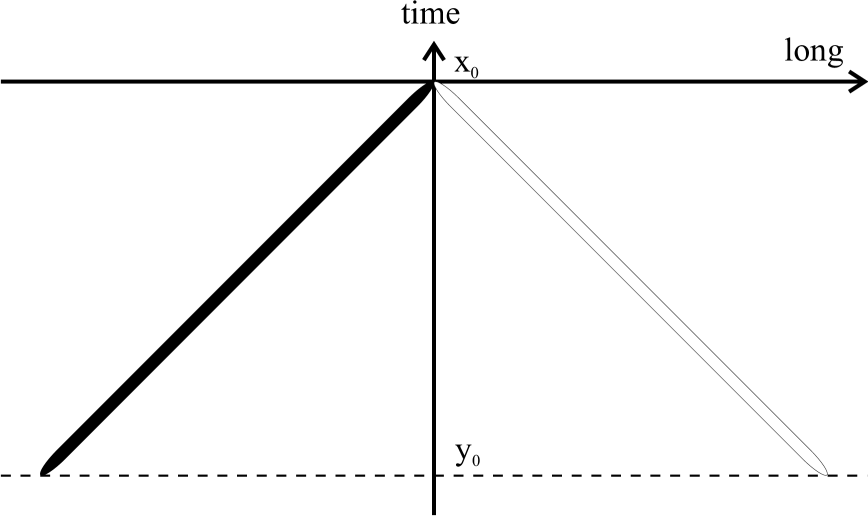
Figure 2: The two contributions to equation (30) from the backward light-cone. The white line corresponds to the path-ordered exponential along $\xi_{-}$, the black to that along $\xi_{+}$. The origin of the coordinate system is situated at ($x_{0}$,$x_{3}$). The dashed line represents $t=y_{0}$.

with the definition $\sqrt{2}v_{\pm}=v_{0}\pm v_{3}$ and the change of variables to $A=A(x_{+},x_{-})$. The path-ordered exponentials on the right-hand side are Wilson lines in which the $A_{\pm}$-component is integrated along the $\xi_{\mp}$-coordinate, respectively. As a consequence of relativity, the endpoints of the path in the $\xi_{\pm}$-direction depend on the value of the $x_{\mp}$-coordinate, respectively. The two contributions which come exactly from on the backward light-cone are schematically depicted in figure 2.

Loosening the requirements on the system by admitting a non-zero transverse mass leads to four contributions in the exponent of the analogous expression:

$$\check{G}_{\vec{A}_{T}=\vec{0}}(x_{0},y_{0},x_{3},k_{3},\vec{k}_{T})~{}=~{}{\cal P}\exp\left[i\int_{y_{0}-x_{0}}^{0}d\xi_{0}\right.\times~{}$$

$$~{}~{}~{}\times\left(\rho^{+}\left\{\sqrt{2}A_{+}(x_{+},x_{-}+\sqrt{2}\xi_{0})+k_{3}\right\}\rho^{+}+\rho^{-}\left\{\sqrt{2}A_{-}(x_{+}+\sqrt{2}\xi_{0},x_{-})-k_{3}\right\}\rho^{-}+\right.~{}$$

$$~{}~{}~{}+\left.\left.\rho^{+}\gamma^{0}\{\gamma^{J}k_{J}-m\}e^{+2\xi_{0}\partial_{3}(x)}\rho^{-}+\rho^{-}\gamma^{0}\{\gamma^{J}k_{J}-m\}e^{-2\xi_{0}\partial_{3}(x)}\rho^{+}\right)\right]$$ (31)

where use has been made of the idempotency of the projectors and of the relation $\rho^{\pm}\gamma^{0}\{\gamma^{J}k_{J}-m\}=\gamma^{0}\{\gamma^{J}k_{J}-m\}\rho^{\mp}$. In the terms involving the transverse mass – note that $[\gamma^{0}(\gamma^{J}k_{J}-m)]^{2}={m_{T}}^{2}$ – the translation operators do not meet their inverse and hence do not drop out. A resummation of this expression for small transverse mass $m_{T}$ yields:

$$\check{G}_{\vec{A}_{T}=\vec{0}}(x_{0},y_{0},x_{3},k_{3},\vec{k}_{T})~{}=~{}{\cal P}\exp\left[i\int_{y_{0}-x_{0}}^{0}d\xi_{0}\check{G}_{\vec{A}_{T}=\vec{0}}^{m_{T}=0}(x_{0},x_{0}+\xi_{0},x_{3},k_{3})\right.\times~{}$$

$$~{}~{}~{}\times\left(\rho^{+}\gamma^{0}\{\gamma^{J}k_{J}-m\}e^{+2\xi_{0}\partial_{3}(x)}\rho^{-}+\rho^{-}\gamma^{0}\{\gamma^{J}k_{J}-m\}e^{-2\xi_{0}\partial_{3}(x)}\rho^{+}\right)\times~{}$$

$$~{}~{}~{}\times\left.\check{G}_{\vec{A}_{T}=\vec{0}}^{m_{T}=0}(x_{0}+\xi_{0},x_{0},x_{3},k_{3})\right]\check{G}_{\vec{A}_{T}=\vec{0}}^{m_{T}=0}(x_{0},y_{0},x_{3},k_{3}),$$ (32)

where $\check{G}_{\vec{A}_{T}=\vec{0}}^{m_{T}=0}(x_{0},y_{0},x_{3},k_{3})$ has been taken from equation (30). Therefore, the lowest (zero) order term in an expansion of the above expression in the transverse mass equals the result for vanishing transverse mass. The first order expression reads:

$$\check{G}^{(1)}(x_{0},y_{0},x_{3},k_{3},\vec{k}_{T})=\sum_{\pm}ie^{\mp ik_{3}(x_{0}-y_{0})}\int_{y_{0}-x_{0}}^{0}d\xi_{0}e^{\mp 2i[k_{3}+i\partial(x)]\xi_{0}}\check{G}^{(1)\pm\mp}_{\vec{A}_{T}=\vec{0}},$$ (33)

where the sum over the contribution with the upper signs and that with the lower signs is taken:

$$\check{G}^{(1)+-}_{\vec{A}_{T}=\vec{0}} = {\cal P}\exp\left\{i\int_{\sqrt{2}\xi_{0}}^{0}dz_{-}A_{+}(x_{+},x_{-}+z_{-})\right\}\rho^{+}\gamma^{0}\{\gamma^{J}k_{J}-m\}\rho^{-}\times~{}$$

$$\times{\cal P}\exp\left\{i\int_{\sqrt{2}(y_{0}-x_{0}-\xi_{0})}^{0}dz_{+}A_{-}(x_{+}+z_{+},x_{-}+\sqrt{2}\xi_{0})\right\},~{}$$

$$\check{G}^{(1)-+}_{\vec{A}_{T}=\vec{0}} = {\cal P}\exp\left\{i\int_{\sqrt{2}\xi_{0}}^{0}dz_{+}A_{-}(x_{+}+z_{+},x_{-})\right\}\rho^{-}\gamma^{0}\{\gamma^{J}k_{J}-m\}\rho^{+}\times~{}$$ (34)

$$\times{\cal P}\exp\left\{i\int_{\sqrt{2}(y_{0}-x_{0}-\xi_{0})}^{0}dz_{-}A_{+}(x_{+}+\sqrt{2}\xi_{0},x_{-}+z_{-})\right\}.$$

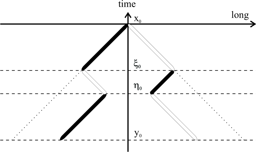
Figure 3: The two contributions to the equations (34) or (35) respectively but for the second order. The white lines correspond to path-ordered exponentials along $z_{-}$, the black to those along $z_{+}$. This figure also represents equation (38) but where the black and the white lines stand for simple integration-paths. In all cases, the kinks are found at $t=\xi_{0}$ and $t=\eta_{0}$, i.e., where the ”transverse” matrices are inserted. The origin of the coordinate system is situated at ($x_{0}$,$x_{3}$). The dashed lines represent lines of constant time. The dotted lines stand for the backward light-cone.

The second order is sketched in figure 3. The kinks appear where the $m_{T}$-terms are inserted. Now, there are not only contributions from on the backward light-cone but also from everywhere within. The different orders in the expansion are weighted by powers of $m_{T}$ according to the number of insertions and thus with the same weight wherever the kink is positioned.

For large transverse mass $m_{T}$ the adequate expansion would be given by an expression analogous to the weak-field case (section II.2.1) but without transverse components of the field.

II.3.2 Gauge fields with dominant longitudinal and temporal gradients

Taking the transverse components of the gauge field into account, too, but where the dependence on time and the longitudinal components is still more pronounced, the previous first-order expressions are modified to yield:

$$\check{G}^{(1)+-} = {\cal P}\exp\left\{i\int_{\sqrt{2}\xi_{0}}^{0}dz_{-}A_{+}(x_{+},x_{-}+z_{-})\right\}\rho^{+}{\cal M}_{T}(x_{+},\sqrt{2}\xi_{0}+x_{-})\rho^{-}\times~{}$$

$$\times{\cal P}\exp\left\{i\int_{\sqrt{2}(y_{0}-x_{0}-\xi_{0})}^{0}dz_{+}A_{-}(x_{+}+z_{+},x_{-}+\sqrt{2}\xi_{0})\right\},~{}$$

$$\check{G}^{(1)-+} = {\cal P}\exp\left\{i\int_{\sqrt{2}\xi_{0}}^{0}dz_{+}A_{-}(x_{+}+z_{+},x_{-})\right\}\rho^{-}{\cal M}_{T}(\sqrt{2}\xi_{0}+x_{+},x_{-})\rho^{+}\times~{}$$ (35)

$$\times{\cal P}\exp\left\{i\int_{\sqrt{2}(y_{0}-x_{0}-\xi_{0})}^{0}dz_{-}A_{+}(x_{+}+\sqrt{2}\xi_{0},x_{-}+z_{-})\right\},$$

with ${\cal M_{T}}(x_{+},x_{-})=\gamma^{0}[\gamma^{J}k_{J}-m+\gamma^{J}A_{J}(x_{+},x_{-})]$, the contribution from the transverse vector components. All ingredients needed in order to put together the full expression in analogy to equation (32) can always be read off from the first-order equations, here and in the following. The main difference with respect to the previous section is that now the trajectories that have a kink at a given point are no longer weighted uniformly with $\gamma^{0}\{\gamma^{J}k_{J}-m\}$ but according to the value of $\gamma^{0}\{\gamma^{J}A_{J}(x_{+},x_{-})+\gamma^{J}k_{J}-m\}$ at the kink $(x_{+},x_{-})$ or, in higher order terms, the various kinks (see figure 3).

In case the transverse components of the field should be dominant compared to the temporal and longitudinal components one can start out with equation (29) and resum the terms involving the transverse gauge field:

$$\check{G}(x_{0},y_{0},x_{3},k_{3},\vec{k}_{T})=~{}$$ (36)

$$= {\cal P}\exp\left[i\int_{y_{0}}^{x_{0}}d\xi_{0}\check{G}_{A_{0,3}=0}(x_{0},\xi_{0},x_{3},k_{3},\vec{k}_{T})U_{3}(x_{0}-\xi_{0})\gamma^{0}[\gamma^{3}k_{3}+\gamma\cdot\tilde{A}(\xi_{0},x_{3})]\right.\times~{}$$

$$\times\left.U_{3}(\xi_{0}-x_{0})\check{G}_{A_{0,3}=0}(\xi_{0},x_{0},x_{3},k_{3},\vec{k}_{T})\right]\check{G}_{A_{0,3}=0}(x_{0},y_{0},x_{3},k_{3},\vec{k}_{T}),$$

with the definition for the four-vectors without transverse components $\tilde{v}^{\mu}=(v^{0},0,0,v^{3})$ and where:

$$\check{G}_{A_{0,3}=0}(x_{0},y_{0},x_{3},k_{3},\vec{k}_{T})~{}=~{}{\cal P}\exp\left\{\frac{i}{\sqrt{2}}\int_{\sqrt{2}(y_{0}-x_{0})}^{0}d\xi_{0}\right.\times~{}$$

$$~{}~{}~{}\times\left.\left(\rho^{+}{\cal M_{T}}(x_{+},x_{-}+\xi_{0})\rho^{-}e^{+\sqrt{2}\xi_{0}\partial_{3}(x)}\right.\right.+\left.\left.\rho^{-}{\cal M}_{T}(x_{+}+\xi_{0},x_{-})\rho^{+}e^{-\sqrt{2}\xi_{0}\partial_{3}(x)}\right)\right\}.$$ (37)

The most important difference between the equations (37) and (30) is the fact, that a decomposition into two terms involving exponentials without Clifford matrices in the argument is not possible. However, because of the alternating occurrence of the projectors $\rho^{\pm}$, the expansion of this path-ordered exponential leads to two contributions per order: one with $\rho^{+}$ on the left-hand side and the other with a $\rho^{-}$. See, for example, the second-order term: Together with the projectors, the translation operators appear in an alternating manner. This ensures that only contributions from on or within the backward light-cone are taken into account. That can be seen best after putting all translation operators to the right:

$$\check{G}^{(2)}_{A_{0,3}=0}(x_{0},y_{0},x_{3},k_{3},\vec{k}_{T})~{}=~{}\frac{i}{\sqrt{2}}\int_{\sqrt{2}(y_{0}-x_{0})}^{0}d\xi_{0}\frac{i}{\sqrt{2}}\int_{\sqrt{2}(y_{0}-x_{0}-\xi_{0})}^{0}d\eta_{0}\times~{}$$

$$~{}~{}~{}\times\left[\rho^{+}{\cal M_{T}}(x_{+},\xi_{0}+x_{-})\right.{\cal M}_{T}(x_{+}+\eta_{0},\xi_{0}+x_{-})\rho^{-}e^{-\sqrt{2}\eta_{0}\partial_{3}(x)}+~{}$$

$$~{}~{}~{}~{}+\rho^{-}{\cal M}_{T}(\xi_{0}+x_{+},x_{-})\left.{\cal M}_{T}(\xi_{0}+x_{+},\eta_{0}+x_{-})\rho^{+}e^{+\sqrt{2}\eta_{0}\partial_{3}(x)}\right]$$ (38)

The fact that there are no contributions to the propagator from outside the backward light-cone, consistent with relativity, also persists in the general case (see section II.1 and figure 3).

II.3.3 Gauge field of one time-like curvilinear coordinate

The Green’s functions obtained in field were equal to the retarded propagator only for a field depending on one time-like curvilinear coordinate $n\cdot x$ with $n^{2}>0$. Now one is in the position to give the retarded propagators for gauge fields as functions of one space- ($n^{2}<0$) or light-like ($n^{2}=0$) curvilinear coordinate, too. In order to investigate the different situations it is only necessary to look at one special choice for $n$ in each case, because $n^{2}$ is a Lorentz scalar. For the time-like case $n^{\mu}=(1,0,0,0)$ had been chosen, for the space-like $n^{\mu}=(0,0,0,1)$, and for the light-like $n^{\mu}=(1,0,0,-1)/\sqrt{2}$.

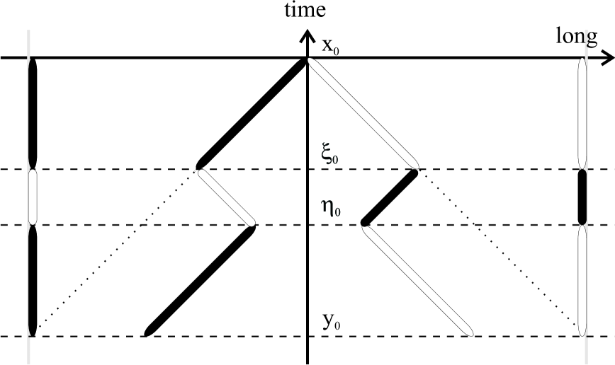
Figure 4: The two contributions in the case of a purely time-dependent field. The sloped white lines correspond to path-ordered exponentials along $z_{-}$, the black to those along $z_{+}$. The kinks are found at $t=\xi_{0}$ and $t=\eta_{0}$, i.e., where the ${\cal M}_{T}$ are inserted. The origin of the coordinate system is situated at ($x_{0}$,$x_{3}$). The dashed lines represent lines of constant time. Along these the black and white lines in the direction of the light-cone coordinates are projected onto the vertical ones at the sides of the figure. These projections represent the paths along which the path-ordered exponentials are actually evaluated in the purely time-dependent case. The dotted lines stand for the backward light-cone.

As already stated before, the time-like case is equivalent to the lowest-order expansion in the spatial gradient of equation (25). A reason for this particularly compact form can be read off figure 4. The contributions to the propagator may be projected along straights of constant time, i.e., the same coordinate for which the retarded propagator’s boundary conditions and hence the variable for the outer integrations are given.

II.3.4 Gauge field of one space-like curvilinear coordinate

If the gauge field is merely a function of a space-like curvilinear coordinate, say $x_{3}$, equations (35) can be rewritten as:

$$\check{G}^{(1)+-}=~{}$$

$$= {\cal P}\exp\left\{i\sqrt{2}\int_{\xi_{0}}^{0}dz_{3}A_{+}(x_{3}-z_{3})\right\}\rho^{+}{\cal M}_{T}(x_{3}-\xi_{0})\rho^{-}{\cal P}\exp\left\{i\sqrt{2}\int_{y_{0}-x_{0}}^{\xi_{0}}dz_{3}A_{-}(x_{3}+z_{3})\right\},~{}$$

$$\check{G}^{(1)-+}=~{}$$

$$= {\cal P}\exp\left\{i\sqrt{2}\int_{\xi_{0}}^{0}dz_{3}A_{-}(x_{3}+z_{3})\right\}\rho^{-}{\cal M}_{T}(x_{3}+\xi_{0})\rho^{+}{\cal P}\exp\left\{i\sqrt{2}\int_{y_{0}-x_{0}}^{\xi_{0}}dz_{3}A_{+}(x_{3}-z_{3})\right\}.~{}$$

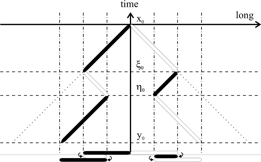
Figure 5: The two contributions in equations (II.3.4) but for the second order. The sloped white lines correspond to path-ordered exponentials along $z_{-}$, the black to those along $z_{+}$. The kinks are found at $t=\xi_{0}$ and $t=\eta_{0}$, i.e., where the ${\cal M}_{T}$ are inserted. The origin of the coordinate system is situated at ($x_{0}$,$x_{3}$). The dashed lines represent lines of constant time. The dotted lines stand for the backward light-cone. The dash-dotted lines mark straights of equal longitudinal coordinate. Along those the black and white lines in the direction of the light-cone coordinates are projected onto the horizontal ones at the bottom of the figure. These represent the paths along which the path-ordered exponentials in the equations (II.3.4) are actually evaluated.

where the variable in the argument of the gauge field has been kept as $A(x_{3})$. As can be seen from this expression and also as indicated in figure 5 the field is integrated back and forth over the longitudinal coordinate while the phase factors are still functions of time [see equation (33)]. To the contrary, the respective Green’s function derived for this case in field which is not a propagator, exhibits a different form, because a different boundary condition had been imposed there.

II.3.5 Gauge field of one light-like curvilinear coordinate

For a gauge field being a function of the light-like coordinate $x_{-}$, the equations (35) simplify to:

$$\check{G}^{(1)+-} = {\cal P}\exp\left\{i\int_{\sqrt{2}\xi_{0}}^{0}dz_{-}A_{+}(x_{-}+z_{-})\right\}\rho^{+}{\cal M}_{T}(\sqrt{2}\xi_{0}+x_{-})\rho^{-}\times~{}$$

$$\times\exp\left\{-i\sqrt{2}(y_{0}-x_{0}-\xi_{0})A_{-}(x_{-}+\sqrt{2}\xi_{0})\right\},~{}$$

$$\check{G}^{(1)-+} = \exp\left\{-i\sqrt{2}\xi_{0}A_{-}(x_{-})\right\}\rho^{-}{\cal M}_{T}(x_{-})\rho^{+}{\cal P}\exp\left\{i\int_{\sqrt{2}(y_{0}-x_{0}-\xi_{0})}^{0}dz_{-}A_{+}(x_{-}+z_{-})\right\}.~{}$$

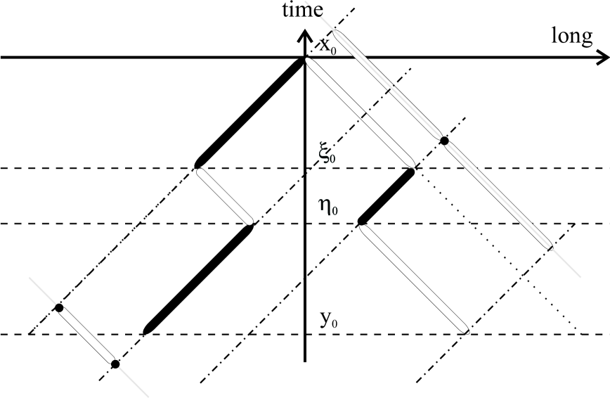
Figure 6: The two contributions in the equations (II.3.5) but for the second order. Of the lines on and inside the backward light-cone (dotted) the white correspond to path-ordered exponentials along $z_{-}$, the black to those along $z_{+}$. The kinks are found at $t=\xi_{0}$ and $t=\eta_{0}$, i.e., where the ${\cal M}_{T}$ are inserted. The origin of the coordinate system is situated at ($x_{0}$,$x_{3}$). The dashed lines represent lines of constant time. The dash-dotted lines mark straights of constant $z_{-}$. Along those the black and white lines inside and on the backward light-cone are projected. These projected lines represent the paths along which the path-ordered exponentials in the equations (II.3.5) are actually evaluated. Especially the black lines are projected onto points which leads to simple phases as the field remains constant.

Here, one of the two path-ordered exponentials per addend becomes a simple phase. It is always the one, which is integrated along $z_{+}$ with $z_{-}$ kept fixed. As the entire argument is only a function of $z_{-}$ it can be taken out of the integral which no longer needs path-ordering and thus only gives a time difference. In figure 6 these phase factors are the contributions parallel to the direction of projection. Therefore, they are each mapped onto a point. The solution presented above is of the form relevant in a field theory with standard quantisation. The respective expression for the homogeneous solution of the Dirac equation in the case of retarded boundary conditions along the light cone was given in field .

II.3.6 Longitudinally boost-invariant gauge fields

A case of particular interest in ultrarelativistic heavy-ion collisions is that of a gauge field which is invariant under longitudinal Lorentz transformations, although this requirement often imposes further limitations on the configurations of the gauge field. Independent of this reasoning, usually also a dependence on the transverse coordinates is present. Here the simpler case is sufficient to clarify the main features. As in the forward light-cone $\tau=\sqrt{t^{2}-z^{2}}>0$, it does not lead to ambiguities to replace it by half its square $x_{+}x_{-}$: $A_{\pm}=x_{\pm}a_{\pm}(x_{+}x_{-})$ and $\vec{A}_{T}=\vec{A}_{T}(x_{+}x_{-})$. Therefore the equations (35) become:

$$\check{G}^{(1)+-} = {\cal P}\exp\left\{i\int_{x_{+}(x_{-}+\sqrt{2}\xi_{0})}^{x_{+}x_{-}}d\zeta a_{+}(\zeta)\right\}\rho^{+}{\cal M}_{T}[x_{+}(x_{-}+\sqrt{2}\xi_{0})]\rho^{-}\times~{}$$

$$\times{\cal P}\exp\left\{i\int^{x_{+}(x_{-}+\sqrt{2}\xi_{0})}_{[\sqrt{2}(y_{0}-\xi_{0})-x_{+}](x_{-}+\sqrt{2}\xi_{0})}d\zeta a_{-}(\zeta)\right\},~{}$$

$$\check{G}^{(1)-+} = {\cal P}\exp\left\{i\int_{(x_{+}+\sqrt{2}\xi_{0})x_{-}}^{x_{+}x_{-}}d\zeta a_{+}(\zeta)\right\}\rho^{-}{\cal M}_{T}[(x_{+}+\sqrt{2}\xi_{0})x_{-}]\rho^{+}\times~{}$$ (41)

$$\times{\cal P}\exp\left\{i\int^{(x_{+}+\sqrt{2}\xi_{0})x_{-}}_{(x_{+}+\sqrt{2}\xi_{0})[\sqrt{2}(y_{0}-\xi_{0})-x_{+}]}d\zeta a_{+}(\zeta)\right\}$$

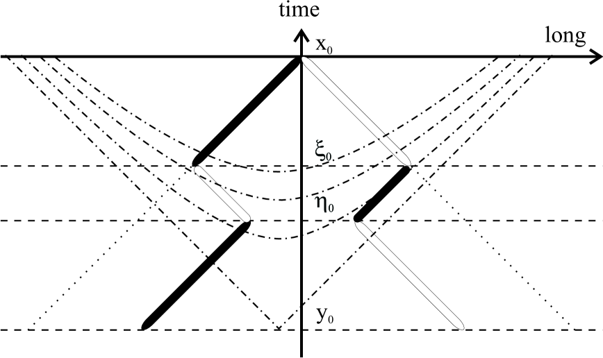
Figure 7: The two contributions in the equations (41) but for the second order. The white lines correspond to path-ordered exponentials along $z_{-}$, the black to those along $z_{+}$. The kinks are found at $t=\xi_{0}$ and $t=\eta_{0}$, i.e., where the ${\cal M}_{T}$ are inserted. The origin of the coordinate system is situated at ($x_{0}$,$x_{3}$). The dashed lines represent lines of constant time. The dotted lines stand for the backward light-cone. The dash-dotted hyperbolas are characterised by constant proper time $\tau$ and hence constant values of the gauge field $A$. Mark that in general there can be an offset between the origin of the coordinate system for these curves (0,0) and that in which the propagator is obtained ($x_{0}$,$x_{3}$). Therefore, the propagator does not exhibit the symmetry properties of the field.

It can be seen from these expressions that the longitudinal boost-invariance of the vector potential does not lead to great simplifications. In fact the propagator itself does not become boost-invariant. The reason for this is that the boundary condition for the retarded propagator is not invariant under longitudinal boosts. From figure 7 it becomes evident as well that the problem does not exhibit the symmetry of the field. Nevertheless, there are simplifications for the homogeneous solution $G_{H}$.

II.4 Ultrarelativistic heavy-ion collisions

A standard way to describe an ultrarelativistic heavy-ion collision is to begin with a current of colour charges moving along the light-cone kr . In order to obtain the classical gauge field the Yang-Mills equations have to be solved in the presence of this current. In Lorenz gauge the field consists of two different contributions.

One of them is made up of the Weizsäcker-Williams sheets. These correspond to the Coulomb fields of the different colour charges boosted into the closure of the Lorentz group. Therewith they become $\delta$-distributions in the light-cone coordinates. This approximation is justified for the description of particles with low longitudinal momentum (mid-rapidity). On the one hand they have a low resolution in this direction. On the other they cannot be comovers of the charges on the light-cone. For comoving particles the plane wave expansion would not be applicable baltz .

The other contribution is the radiation field in the forward light-cone $A^{rad}$. By virtue of longitudinally boost-invariant boundary conditions on the light cone, it is sometimes taken as being invariant under longitudinal boosts, too. However, this is not necessarily the case. But anyway, as has been seen in section II.3.6, there are no fundamental simplifications for the propagator. Thus this assumption will not be taken into account in the following discussion.

In Lorenz gauge, the Weizsäcker-Williams contribution to the gauge-field takes the form:

$$A_{+}^{WW}(x) = -\frac{g}{2\pi}\sum_{n_{L}=1}^{N_{L}}t_{a}(t_{a}^{L})_{n_{L}}\delta\left[x_{-}-(b_{-}^{L})_{n_{L}}\right]\ln\lambda\left|\vec{x}_{T}-(\vec{b}_{T}^{L})_{n_{L}}\right|,~{}$$

$$A_{-}^{WW}(x) = -\frac{g}{2\pi}\sum_{n_{R}=1}^{N_{R}}t_{a}(t_{a}^{R})_{n_{R}}\delta\left[x_{+}-(b_{+}^{R})_{n_{R}}\right]\ln{\lambda\left|\vec{x}_{T}-(\vec{b}_{T}^{R})_{n_{R}}\right|}.$$ (42)

There is no contribution to the transverse components. $\lambda$ is an arbitrary constant, regularising the logarithm which does not appear in quantities like the field tensor. The $t_{a}$ are the generators of $SU(3)_{c}$. The $(t_{a}^{L,R})_{n}$ represent the colour of the charges.

In general, the presence of a second nucleus leads to a precession of the charges of the first nucleus and vice versa which is a manifestation of the covariant conservation of the current. This leads to further sheet-like contributions to the gauge field which can be combined with the Weizsäcker-Williams fields by modifying the charges. Up to the next-to-leading order in perturbation theory they read kr :

$$(t_{a}^{L})_{n_{L}} = (t_{a}^{L})_{n_{L}}^{in}-\alpha_{S}\sum_{n_{R}=1}^{N_{R}}f_{abc}(t_{b}^{L})_{n_{L}}^{in}(t_{c}^{R})_{n_{R}}^{in}\theta\left[x_{+}-(b_{+}^{R})_{n_{R}}\right]\ln\lambda|\vec{x}_{T}-(\vec{b}_{T}^{R})_{n_{R}}|+{\cal O}({\alpha_{S}}^{2}),~{}$$

$$(t_{a}^{R})_{n_{R}} = (t_{a}^{R})_{n_{R}}^{in}+\alpha_{S}\sum_{n_{L}=1}^{N_{L}}f_{abc}(t_{b}^{L})_{n_{L}}^{in}(t_{c}^{R})_{n_{R}}^{in}\theta\left[x_{-}-(b_{-}^{L})_{n_{L}}\right]\ln\lambda|\vec{x}_{T}-(\vec{b}_{T}^{L})_{n_{L}}|+{\cal O}({\alpha_{S}}^{2}).~{}$$

with the initial colours $(t_{a}^{L,R})^{in}_{n_{L,R}}$. To all orders, the modifications amount to Wilson lines over the gauge field along the branches of the light cone. Hence, the precession terms are absent in adequate, i.e., light-cone gauges. In order to ensure colour neutrality of each nucleus the following relations have to be satisfied: $\sum_{n_{L}=1}^{N_{L}}t_{a}(t_{a}^{L})_{n_{L}}^{in}=0=\sum_{n_{R}=1}^{N_{R}}t_{a}(t_{a}^{R})_{n_{R}}^{in}$. Frequently, pairs of two charges belonging to the same nucleus are assigned to each other to form a colour-neutral dipole. Ultimately, higher-order perturbative calculations for the gauge field as solution of the Yang-Mills equations are only of value in the presence of hard energy- or short time-scales. Up to now, non-perturbative solutions for this problem have been obtained only in transverse lattice calculations transverse . In any case, the general form of the field – continuous inside the forward light-cone and singular but integrable on the forward light-cone – allows to express the retarded propagator by a finite number of addends. Resumming the terms involving the Weizsäcker-Williams-like contributions together with the longitudinal derivatives in the homogeneous part in equation (II) yields:

$${\cal P}\exp\left\{i\int_{y_{0}}^{x_{0}}d\xi_{0}\gamma^{0}[i\gamma^{j}\partial_{j}(x)+\gamma^{j}k_{j}+\gamma\cdot A^{WW}(\xi_{0},\vec{x})+\gamma\cdot A^{rad}(\xi_{0},\vec{x})-m]\right\}=~{}$$ (44)

$$= {\cal P}\exp\left[i\int_{y_{0}}^{x_{0}}d\xi_{0}{\cal P}\exp\left\{i\int_{\xi_{0}}^{x_{0}}dz_{0}\gamma^{0}[i\gamma^{3}\partial_{3}(x)+\gamma\cdot A^{WW}(z_{0},\vec{x})]\right\}\right.\times~{}$$

$$~{}~{}~{}~{}~{}~{}~{}~{}~{}~{}~{}~{}~{}~{}~{}~{}~{}~{}~{}~{}\times\gamma^{0}[i\gamma^{J}\partial_{J}(x)+\gamma^{j}k_{j}+\gamma\cdot A^{rad}(\xi_{0},\vec{x})-m]\times~{}$$

$$~{}~{}~{}~{}~{}~{}~{}~{}~{}~{}~{}~{}~{}~{}~{}~{}~{}\times\left.{\cal P}\exp\left\{i\int^{\xi_{0}}_{x_{0}}dz_{0}\gamma^{0}[i\gamma^{3}\partial_{3}(x)+\gamma\cdot A^{WW}(z_{0},\vec{x})]\right\}\right]\times~{}$$

$$\times{\cal P}\exp\left\{i\int_{y_{0}}^{x_{0}}d\xi_{0}\gamma^{0}[i\gamma^{3}\partial_{3}(x)+\gamma\cdot A^{WW}(\xi_{0},\vec{x})]\right\}$$

The path-ordered exponentials containing the Weizsäcker-Williams contribution to the vectorpotential can be written in the form of equation (30), because they do not contain any transverse components. Note that $k_{3}=0$ has to be used as the longitudinal momentum has been kept inside the outer path-ordered exponential. Hence, after replacing $A^{WW}$ by equations (42) and carrying out the path-ordered integration, one obtains:

$${\cal P}\exp\left\{i\int_{y_{0}}^{x_{0}}d\xi_{0}\gamma^{0}[i\gamma^{3}\partial_{3}(x)+\gamma\cdot A^{WW}(\xi_{0},\vec{x})]\right\}=~{}$$ (45)

$$= \rho^{+}{\cal P}\prod_{n_{L}=1}^{N_{L}}\exp\left[ia_{n_{L}}^{L}(\vec{x}_{T})\left\{\theta[x_{-}-(b_{-}^{L})_{n_{L}}]-\theta[y_{-}-(b_{-}^{L})_{n_{L}}]\right\}\right]e^{-(x_{0}-y_{0})\partial_{3}(x)}+~{}$$

$$+ \rho^{-}{\cal P}\prod_{n_{R}=1}^{N_{R}}\exp\left[ia_{n_{R}}^{R}(\vec{x}_{T})\left\{\theta[x_{+}-(b_{+}^{R})_{n_{R}}]-\theta[y_{+}-(b_{+}^{R})_{n_{R}}]\right\}\right]e^{+(x_{0}-y_{0})\partial_{3}(x)},$$

with $2\pi a_{n_{L,R}}^{L,R}=-gt_{a}(t_{a}^{L,R})_{n_{L,R}}\ln\lambda\left|\vec{x}_{T}-(\vec{b}_{T}^{L,R})_{n_{L,R}}\right|$. It has been assumed that the sums in equation (42) are ordered in such a way that, if $m_{L}>n_{L}$ then $(b_{-}^{L})_{m_{L}}>(b_{-}^{L})_{n_{L}}$ and likewise if $m_{R}>n_{R}$ then $(b_{+}^{R})_{m_{R}}>(b_{+}^{R})_{n_{R}}$. The same is to hold for the products in the previous equation and has been indicated by the ${\cal P}$. In contrast to equation (30), the translation operators are explicitely shown above. There they had been absorbed in equation (28).

Making repeated use of the relation $f[\theta(+x)]=\theta(+x)f(1)+\theta(-x)f(0)$ and subsequent simplifications lead to:

$${\cal P}\exp\left\{i\int_{y_{0}}^{x_{0}}d\xi_{0}\gamma^{0}[i\gamma^{3}\partial_{3}(x)+\gamma\cdot A^{WW}(\xi_{0},\vec{x})]\right\}=~{}$$ (46)

$$= \rho^{+}{\cal P}\prod_{n_{L}=1}^{N_{L}}\left[1+\left\{\theta[x_{-}-(b_{-}^{L})_{n_{L}}]-\theta[y_{-}-(b_{-}^{L})_{n_{L}}]\right\}\right.\times~{}$$

$$\times\left.\left\{\theta(y_{0}-x_{0})\exp[+ia_{n_{L}}^{L}(\vec{x}_{T})]-\theta(x_{0}-y_{0})\exp[-ia_{n_{L}}^{L}(\vec{x}_{T})]-1\right\}\right]e^{-(x_{0}-y_{0})\partial_{3}(x)}+~{}$$

$$+ \rho^{-}{\cal P}\prod_{n_{R}=1}^{N_{R}}\left[1+\left\{\theta[x_{+}-(b_{+}^{R})_{n_{R}}]-\theta[y_{+}-(b_{+}^{R})_{n_{R}}]\right\}\right.\times~{}$$

$$\times\left.\left\{\theta(y_{0}-x_{0})\exp[+ia_{n_{R}}^{R}(\vec{x}_{T})]-\theta(x_{0}-y_{0})\exp[-ia_{n_{R}}^{R}(\vec{x}_{T})]-1\right\}\right]e^{+(x_{0}-y_{0})\partial_{3}(x)}$$

In ultrarelativistic heavy-ion collisions, the colliding nuclei are highly Lorentz-contracted. Therefore, in the infinite-energy limit $\gamma\rightarrow\infty$, the ”longitudinal impact parameters” $(b_{\pm}^{L,R})_{n_{R,L}}$ go to zero like $\gamma^{-1}$. However, care has to be taken, as important, because qualitatively different contributions to observables could be neglected, although the expression for the propagator in this limit would still be correct. Taking the limit, the factors involving the differences of the step functions become the same for all terms of the first and the second contribution respectively, and thus can be factored out. Afterwards, the idempotency of the step functions remaining in the product can be used to split each contribution into three addends which can be recombined in pairs:

$${\cal P}\exp\left\{i\int_{y_{0}}^{x_{0}}d\xi_{0}\gamma^{0}[i\gamma^{3}\partial_{3}(x)+\gamma\cdot A^{WW}(\xi_{0},\vec{x})]\right\}={\cal P}\exp\left\{-\int_{y_{0}}^{x_{0}}d\xi_{0}\gamma^{0}\gamma^{3}\partial_{3}(x)\right\}+~{}$$

$$+ T^{L}(x,\pm)[\theta(x_{-})-\theta(y_{-})]e^{-(x_{0}-y_{0})\partial_{3}(x)}+T^{R}(x,\pm)[\theta(x_{+})-\theta(y_{+})]e^{+(x_{0}-y_{0})\partial_{3}(x)},~{}$$

with:

$$T^{L}(x,\pm)+\rho^{+}=\rho^{+}(\pm 1)^{N_{L}}{\cal P}\prod_{n_{L}=1}^{N_{L}}\exp[\pm ia_{n_{L}}^{L}(\vec{x}_{T})]~{}$$

$$T^{R}(x,\pm)+\rho^{-}=\rho^{-}(\pm 1)^{N_{R}}{\cal P}\prod_{n_{R}=1}^{N_{R}}\exp[\pm ia_{n_{R}}^{R}(\vec{x}_{T})],$$ (48)

where $\pm$ in the argument indicates the sign of $x_{0}-y_{0}$. If the two nuclei are modeled by means of dipoles $N_{L}$ and $N_{R}$ are even and the overall factors with the sign are obsolete. What is left of the longitudinal structure of the nuclei is the path-ordering of the products. It would become irrelevant after averaging over all permutations of the charges in which case it would be possible to write the product over the exponentials as simple exponential over the sum of the contributions.

Putting equation (LABEL:recombi) into equation (44) allows for the reconstruction of the homogeneous part of the retarded propagators in the radiation field $G^{rad}_{H}$:

$$G^{rad}_{H}(x,y,\vec{k})={\cal P}\exp\left\{i\int_{y_{0}}^{x_{0}}d\xi_{0}\gamma^{0}[i\gamma^{j}\partial_{j}(x)+\gamma^{j}k_{j}+\gamma\cdot A^{rad}(\xi_{0},\vec{x})-m]\right\}$$ (49)

and the final result reads:

$$G_{H}(x,y,\vec{k})=G_{H}^{rad}(x,y,\vec{k})+~{}$$

$$+\int d^{4}\xi G_{H}^{rad}(x,\xi,\vec{k})[T^{L}(\xi,\pm)\delta(\xi_{-})+T^{R}(\xi,\pm)\delta(\xi_{+})]G_{H}^{rad}(\xi,y,\vec{k})+~{}$$

$$+\int d^{4}\xi d^{4}\eta G_{H}^{rad}(x,\xi,\vec{k})T^{L}(\xi,\pm)\delta(\xi_{-})G_{H}^{rad}(\xi,\eta,\vec{k})T^{R}(\eta,\pm)\delta(\eta_{+})G_{H}^{rad}(\eta,y,\vec{k})+~{}$$

$$+\int d^{4}\xi d^{4}\eta G_{H}^{rad}(x,\xi,\vec{k})T^{R}(\xi,\pm)\delta(\xi_{+})G_{H}^{rad}(\xi,\eta,\vec{k})T^{L}(\eta,\pm)\delta(\eta_{-})G_{H}^{rad}(\eta,y,\vec{k}).$$ (50)

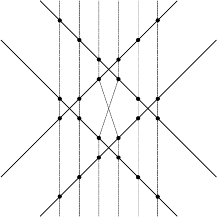
Figure 8: The six contributions to the retarded propagator of highest order in the Weizsäcker-Williams fields of two colliding dipoles. The solid lines depict the trajectories of the charges, the dashed generic integration paths which, in the forward light-cone, correspond to retarded propagators in the radiation field.

When the retarded (advanced) propagator is constructed from this homogeneous part, the minus (plus) sign in the argument of the $T$ has to be taken. Higher orders in the $T$ cannot contribute, because lines of constant $x_{-}$ or $x_{+}$ can only be crossed once (see the discussion above). In the case of two colliding dipoles taking the ultrarelativistic limit in order to obtain equation (LABEL:recombi) keeps only integration paths like the outer two depicted in figure 8. The other, qualitatively different paths, in which interactions with left- and right-movers are intertwined are neglected. With finite ”longitudinal impact parameters”, every charge would have to be treated on its own and the previous equation would contain contributions with up to $N_{L}+N_{R}$ insertions.

For a given field, the retarded propagator in the radiation field could now be obtained with the methods presented earlier in this section. The exact solution for the radiation field would be needed. Finally averaging over all configurations (current and hence field) would yield the desired observables. However, the transverse lattice calculation required at that point is beyond the scope of the present paper.

III Fermion-antifermion pair production

In this section, the findings for the full propagator in a space-time dependent field are interpreted in view of the problem of particle production by vacuum polarisation. Such a calculation can be understood in two different ways. Either the field is an external field in the strict sense, or the field is the self-consistent solution of a set of equations. In the first case it is governed entirely by the characteristics of the physical system without the phenomenon of particle creation. Subsequently it can be used to determine the spectrum of produced particles. An approach of this kind is justified if particle production represents only a perturbation which must be checked eventually. In the second case, given the solution for the set of equations in form of the classical field is known, the question is how many particles were created in the process. Here, the set of equations would include the Yang-Mills equations with an initially present current and the current induced by the fermions and antifermions. In this section the first way is to be pursued, because the back-reaction in the investigated system is suppressed by higher powers of the coupling constant not accompanied by powers of the vector potential.

According to derivation the expectation value for the number of produced pairs can be determined by starting out with a negative energy fermion with four-momentum $q$ corresponding to a positive energy antifermion:

$$\psi_{q}(y)=v(q)e^{-iq\cdot y},$$ (51)

with the unit spinor $v(q)$. After its propagation through the field, calculate its overlap with a positive energy fermion solution with four-momentum $p$:

$$\psi_{p}(x)=u(p)e^{+ip\cdot x},$$ (52)

with the unit spinor $u(p)$. Wave-function solutions of the Dirac equation at $x$ and $y$ are connected by the retarded propagator according to:

$$\psi(x)=\int d^{3}yG_{R}(x,y)\gamma^{0}\psi_{q}(y).$$ (53)

Hence, the required overlap reads:

$$M(p,q)=\int d^{3}xd^{3}y\psi^{\dagger}_{p}(x)G_{R}(x,y)\gamma^{0}\psi_{q}(y).$$ (54)

With the definition of the retarded one-particle scattering-operator ${\cal T}_{R}$

$$G_{R}(x,y)=G_{R}^{0}(x-y)+\int d^{4}\xi d^{4}\eta G_{R}^{0}(x-\xi){\cal T}_{R}(\xi,\eta)G_{R}^{0}(\eta-y),$$ (55)

the overlap can be rewritten as:

$$M(p,q)~{}=~{}\int d^{4}\xi d^{4}\eta\bar{\psi}_{p}(\xi){\cal T}_{R}(\xi,\eta)\psi_{q}(\eta)~{}=~{}\bar{u}(p){\cal T}_{R}(p,-q)v(q),$$ (56)

because $\psi_{q}$ and $\psi_{p}$ are orthogonal to each other and are solutions of the free Dirac equation, whence:

$$\int d^{3}yG_{R}^{0}(x-y)\gamma^{0}\psi_{q}(y) = \psi_{q}(x)~{}$$

$$\int d^{3}y\bar{\psi}_{p}(y)\gamma^{0}G_{R}^{0}(y-x) = \bar{\psi}_{p}(x).$$ (57)

In the last step the definitions of $\psi_{q}$ and $\psi_{p}$ in equations (51) and (52) had been inserted and the integrations carried out. This led to the Fourier transformation of the single-particle scattering operator. The square of this overlap $|M(p,q)|^{2}$ summed/averaged over all colours and spins is equal to the differential expectation value for the number of produced pairs where the particle carries the momentum $p$ and the antiparticle the momentum $q$. After integration over the phase space of the particle (antiparticle) one obtains the spectrum of produced antiparticles (particles). Integration over all momenta finally gives the expectation value for the number of produced pairs:

$$\left<n\right>=\int\frac{d^{3}q}{2(2\pi)^{3}\omega_{q}}\frac{d^{3}p}{2(2\pi)^{3}\omega_{p}}\left|\bar{u}(q){{\cal T}}_{R}(q,-p)v(p)\right|^{2},$$ (58)

where $\omega_{p}=\sqrt{|\vec{p}|^{2}+m^{2}}$ and $\omega_{q}=\sqrt{|\vec{q}|^{2}+m^{2}}$.

In order to address the issue of gauge invariance, rewrite the previous expression as baltz :

$$\left<n\right>=-\int\frac{d^{3}q}{(2\pi)^{3}2\omega_{q}}d^{4}xd^{4}ye^{iq\cdot(x-y)}{\rm tr}\left\{(\gamma\cdot q+m)[i\gamma\cdot\partial(x)-m]G_{+-}(x,y)[i\gamma\cdot\partial(y)-m]\right\},~{}$$

(59)

where the derivatives are only acting on the propagator. The only coloured and hence gauge-dependent part of equation (59) is the propagator, even after taking the trace over its colour indices:

$${\rm tr}\left\{G(x,y)\right\}\rightarrow{\rm tr}\left\{G^{\prime}(x,y)\right\}={\rm tr}\left\{\Omega(x)G(x,y)\Omega^{\dagger}(y)\right\}\neq{\rm tr}\left\{G(x,y)\right\}$$ (60)

III.0.1 Gauge-dependent states / Wilson links

Sometimes, the gauge invariance of the previous expressions is ensured by replacing the gauge-independent free states in equations (51) and (52) by gauge dependent states $\tilde{\psi}$, especially fermion and antifermion solutions in pure gauge fields, i.e., vacuum configurations of the gauge field:

$$\left\{i\gamma\cdot\partial(x)+\Omega(x)[\gamma\cdot\partial(x)\Omega^{\dagger}(x)]-m\right\}\tilde{\psi}(x)=0.$$ (61)

The gauge transformations associated with them cancel those coming from the propagator in equation (54) exactly:

$$\tilde{M}(p,q) = \int d^{3}xd^{3}y\tilde{\psi}^{\dagger}_{p}(x)G_{R}(x,y)\gamma^{0}\tilde{\psi}_{q}(y)\rightarrow\int d^{3}xd^{3}y\tilde{\psi}^{\dagger\prime}_{p}(x)G_{R}^{\prime}(x,y)\gamma^{0}\tilde{\psi}_{q}^{\prime}(y)=~{}$$ (62)

$$= \int d^{3}xd^{3}y\tilde{\psi}^{\dagger}_{p}(x)\Omega^{\dagger}(x)\Omega(x)G_{R}(x,y)\Omega^{\dagger}(y)\gamma^{0}\Omega(y)\tilde{\psi}_{q}(y)=\tilde{M}(p,q)$$

A priori, the gauge in which $\tilde{\psi}(x)$ coincides with a free solution can be chosen arbitrarily, whence it must be specified in order to allow for an interpretation, which therefore is not unique. This goes hand-in-hand with the loss of an interpretation as states with a definite number of partons. In all but the one gauge of reference an arbitrary number of additional gluons is included in them. Further, when deriving equation (58) $q$ and $p$ were the momenta of the fermion and the antifermion, respectively. Here, this correspondence remains obvious only in one gauge, which thus would be singled out.

This method is equivalent to including Wilson lines with the correlators. For an adequate choice of these gauge links – especially their end-points – the gauge transformations connected to them cancel with those of the two-point functions. There the supplementary degree of freedom is the path along which it is evaluated.

III.0.2 Average over the gauge group

A way to guarantee a gauge invariant-expression without sacrificing the requirement of purely fermionic states is given by averaging the expression (59) for the expectation value over all gauges, because every supplementary gauge transformation $\omega(x)$ can then be absorbed by shifting the functional-integral measure:

$$\int[d\Omega]{\rm tr}\left\{\omega(x)G(x,y)\omega^{\dagger}(y)\right\}=\int[d(\omega\Omega)]{\rm tr}\left\{G(x,y)\right\}=\int[d\Omega^{\prime}]{\rm tr}\left\{G(x,y)\right\}.$$ (63)

As a first step, carry out a coordinate transformation from $x$ and $y$ to $\xi=x-y$ and $\zeta=(x+y)/2$. Subsequently look at $d\left<n\right>/d^{4}\xi$. Any SU(N) gauge transformation can be parametrised according to

$$\Omega(x)=\exp\{-it^{a}\theta^{a}(x)\}=\sum_{n=1}^{N}\left|n(x)\right>\left<n(x)\right|\exp\{-i\lambda_{n}(x)\}$$ (64)

with $t^{a}$ the generators of the gauge algebra and where $\lambda_{n}(x)$ are real eigenvalues and $\left|n(x)\right>$ orthonormalised eigenvectors of the matrix $t^{a}\theta^{a}(x)$. Functional integration of $d\left<n\right>/d^{4}\xi$ over the eigenvalues in equation (60) yields a non-zero result for $x=y$:

$$\left.\frac{d\left<\bar{n}\right>}{d^{4}\xi}\right|_{\xi=0} = -\int\frac{d^{3}q}{(2\pi)^{3}2\omega_{q}}d^{4}\zeta\times~{}$$

$$\times{\rm tr}\left\{(\gamma\cdot q+m)\left[i\left.\gamma\cdot\partial(\zeta_{1})\right|_{\zeta_{1}=\zeta}-m\right]G_{+-}(\zeta_{1},\zeta_{2})\left[i\left.\gamma\cdot\partial(\zeta_{2})\right|_{\zeta_{2}=\zeta}-m\right]\right\}~{}$$

Already in its present form the last expression is gauge invariant. Averaging over the eigenvectors $\left|n(x)\right>$ is not needed, because the trace already takes care of colour neutrality. Now the two gauge transformations in equation (60) are evaluated at the same point and drop out of the trace.

This result resembles calculations on the lattice. There the results contain the four-dimensional lattice-volume ${\cal V}$ as an overall factor. Hence, in that case one would look at a quantity like $\left<\bar{n}\right>/{\cal V}$.

With the integrand in momentum space, the previous result becomes:

$$\left.\frac{d\left<\bar{n}\right>}{d^{4}\xi}\right|_{\xi=0} = -\int\frac{d^{3}q}{(2\pi)^{3}2\omega_{q}}\frac{d^{4}l}{(2\pi)^{4}}{\rm tr}\left\{(\gamma\cdot q+m){G_{R}^{0}}^{-1}(l)G_{+-}(l,l){G_{A}^{0}}^{-1}(l)\right\}~{}$$

instead of

$$\left<n\right>=\int\frac{d^{3}q}{(2\pi)^{3}2\omega_{q}}{\rm tr}\left\{(\gamma\cdot q+m){G_{R}^{0}}^{-1}(q)G_{+-}(q,q){G_{A}^{0}}^{-1}(q)\right\},$$ (67)

which would be obtained directly from equation (59).

Making use of equation (5) ($\sigma_{1}=+$, $\sigma_{2}=-$) as well as baltz :

$${\cal T}_{A}(q,p)-{\cal T}_{R}(q,p)=\int\frac{d^{4}k}{(2\pi)^{3}}\delta(k^{2}-m^{2}){\rm sgn}(k_{0}){\cal T}_{R}(q,k)(\gamma\cdot k+m){\cal T}_{A}(k,p)$$ (68)

and:

$$G_{S}(q,p)=\int\frac{d^{4}k}{(2\pi)^{3}}\delta(k^{2}-m^{2})G^{0}_{R}(q){\cal T}_{R}(q,k)(\gamma\cdot k+m){\cal T}_{A}(k,p)G^{0}_{A}(p),$$ (69)

gives:

$$\left.\frac{d\left<\bar{n}\right>}{d^{4}\xi}\right|_{\xi=0}=\int\frac{d^{4}q}{(2\pi)^{4}}\theta(+q_{0})2\pi\delta(q^{2}-m^{2})\frac{d^{4}k}{(2\pi)^{4}}\theta(-k_{0})2\pi\delta(k^{2}-m^{2})\frac{d^{4}l}{(2\pi)^{4}}\times~{}~{}~{}~{}~{}~{}~{}~{}~{}~{}~{}$$

$$\times{\rm tr}\{(\gamma\cdot q+m){\cal T}_{R}(l,k)(\gamma\cdot k+m){\cal T}_{A}(k,l)\}.$$ (70)

This equation can be interpreted as the fermionic current induced by the external field from which the on-shell component ($q^{2}=m^{2}$) is projected out with the extra condition that the current’s momentum is on the mass shell once ($k^{2}=m^{2}$). Opposed to that, in equation (58) the momentum is forced to be on-shell twice.

Under a local gauge transformation $\Omega(x)$, the full propagator transforms homogeneously [see equation (60)]. The considerations concerning gauge invariance remain unchanged, if this behaviour is preserved in an approximation. In the case where, in a given gauge and/or Lorentz frame a certain expansion should be exact, this requirement is trivially satisfied. In general, if the expansion is based on powers of the covariant derivatives and/or the mass, covariance is always ensured. This is the case for equation (30), for expansions of equation (32) if the transverse momentum is omitted, and for approximations like equation (35) if the transverse derivatives are included with ${\cal M}_{T}$ [after adapting equations (28) and (29)]. If the approximate propagator should not transform homogeneously, still a gauge invariant result can be obtained by averaging over all gauges. However, in that case the situation has to be reinvestigated, because the condition $x=y$ need not be sufficient to guarantee gauge invariance there.

III.1 An example

The radiation field in an ultrarelativistic heavy-ion collision has to be determined in transverse lattice calculations which are beyond the scope of the present paper. Hence, the previously determined expressions for the propagator and the quantities derived from it are to be evaluated for a model for the radiation field. Along the lines of the discussion in section II.4 a longitudinally boost-invariant field is chosen:

$$A_{\pm}=\pm a\frac{x_{\pm}}{\tau_{0}}e^{-x_{+}x_{-}/{\tau_{0}}^{2}}.$$ (71)

The Lorenz $\partial\cdot A=0$ and the Fock-Schwinger $x\cdot A=0$ gauge-conditions are satisfied by this field. In its presence the one-particle scattering-operator defined in equation (55) with the propagator according to the lowest order expansion in the transverse components in section II.4 reads:

$${\cal T}_{R}(p,q)=(2\pi)^{2}\delta^{(2)}(\vec{p}_{T}-\vec{q}_{T}){\cal T}_{R}(\tilde{p},\tilde{q})$$ (72)

with:

$$\sqrt{2}{\cal T}_{R}(\tilde{p},\tilde{q})=\gamma_{+}{\cal T}_{R}^{+}(\tilde{p},\tilde{q})+\gamma_{-}{\cal T}_{R}^{-}(\tilde{p},\tilde{q})$$ (73)

where:

$${\cal T}_{R}^{\pm}(\tilde{p},-\tilde{q}) = \mp a\tau_{0}\frac{f(r_{+}r_{-}{\tau_{0}}^{2})}{(r_{+}r_{-}{\tau_{0}}^{2})r_{\pm}}-~{}$$

$$-a^{2}\sum_{\mu\nu}\frac{(\pm ia\tau_{0})^{\mu}}{\mu!}\frac{(\mp ia\tau_{0})^{\nu}}{\nu!}\frac{f[r_{+}r_{-}{\tau_{0}}^{2}/(\mu+\nu+2)]-f[p_{\pm}r_{\mp}{\tau_{0}}^{2}/(\mu+\nu+2)]}{{r_{\pm}}^{2}[(\mu+1)q_{\mp}-(\nu+1)p_{\mp}]},~{}$$

with $r_{\pm}=p_{\pm}+q_{\pm}$. In equation (72) the omnipresent Dirac-distribution, originating from the transverse homogeneity of the field, is factored out. The expressions for the two components of the one-particle scattering-operator can be resummed partially into hypergeometric functions. $f$ involves the exponential-integral function ${\rm Ei}$: $f(\sigma)=\sigma^{2}e^{-\sigma}{\rm Ei}(\sigma)-\sigma.$ In accordance with the discussion in the previous section, the approximation to the retarded propagator used here transforms like the full solutions, i.e., homogeneously. Higher order contributions to the retarded propagator $G_{R}(x,y)$ are also available analytically. They are qualitatively similar to the lowest order investigated here. However, the terms belonging to the different orders cannot be resummed easily. Further, a related approach to the problem of particle production investigated in field turned out to be in good agreement with the full solution.

III.1.1 Gauge-dependent states / Wilson links

An interpretation of equations (72-III.1) put into the integrand of equation (58):

$$\left|\bar{u}(q){\cal T}_{R}(q,-p)v(p)\right|^{2}=\sum_{n}\left[8(p\cdot{\cal T}_{R})(p\cdot{{\cal T}_{R}]}^{\dagger})-4(p\cdot q-m^{2})({\cal T}_{R}\cdot{{\cal T}_{R}}^{\dagger})]\right]$$ (75)

along the lines of the discussion in section III.0.1 would be possible if the gauge of reference was chosen to be the Lorenz or the Fock-Schwinger gauge. Here, in these gauges, the vacuum configuration of the gauge field vanishes identically per definition, whence the fermion solutions $\tilde{\psi}$ in the vacuum configuration coincide with the free solution. The last expression is summed over the eigenvalues $\lambda_{n}$ of the colour matrix $a=\sum_{n}\lambda_{n}\left|n\right>\left<n\right|$.

In the case, where a light-cone gauge, say $A_{+}=0$ was taken, one would have to resort to the expression of the one-particle scattering-operator in that gauge:

${\cal T}_{R}^{-}=0$

and

$${\cal T}_{R}^{+}(\tilde{p},-\tilde{q}) = -2a\tau_{0}\frac{f(r_{+}r_{-}{\tau_{0}}^{2})}{(r_{+}r_{-}{\tau_{0}}^{2})r_{+}}-~{}$$

$$-4a^{2}\sum_{\mu\nu}\frac{(+2ia\tau_{0})^{\mu}}{\mu!}\frac{(-2ia\tau_{0})^{\nu}}{\nu!}\frac{f[r_{+}r_{-}{\tau_{0}}^{2}/(\mu+\nu+2)]-f[p_{+}r_{-}{\tau_{0}}^{2}/(\mu+\nu+2)]}{{r_{+}}^{2}[(\mu+1)q_{-}-(\nu+1)p_{-}]}.~{}$$

In other words, the Wilson line taken along the $x_{-}$-direction becomes unity.

III.1.2 Average over the gauge group

For a calculation according to section III.0.2 one can start in any gauge. In momentum space, the advanced single-particle scattering-operator is linked to the retarded via ${\cal T}_{A}(p,q)=-{\cal T}_{R}^{*}(q,p)$. Starting from equation (III.1.1) the integration over the momentum $l$ and the trace can be executed to yield:

$$\frac{2}{8q_{+}k_{+}}\int\frac{d^{2}\tilde{l}}{(2\pi)^{2}}{\rm tr}\{(\gamma\cdot q+m){\cal T}_{R}(\tilde{l},\tilde{k})(\gamma\cdot k+m){\cal T}_{A}(\tilde{k},\tilde{l})\}=~{}$$

$$= (a\eta)^{2}+\sum_{\mu\nu}\frac{(+2ia\tau_{0})^{\mu}}{\mu!}\frac{(-2ia\tau_{0})^{\nu}}{\nu!}\times~{}$$

$$\times\left(+4i(a\tau_{0})^{3}\left\{\frac{\eta^{2}(\mu+2)+2i{\tau_{0}}^{2}k_{-}\eta}{2{\tau_{0}}^{2}(\mu+2)^{2}(\mu+\nu+3)}-{\tau_{0}}^{2}{k_{-}}^{2}\ln\left[1+i\frac{\eta(\mu+2)}{k_{-}{\tau_{0}}^{2}}\right]\right\}-\right.~{}$$

$$~{}~{}~{}~{}-4i(a\tau_{0})^{3}\left\{\frac{\eta^{2}(\nu+2)+2i{\tau_{0}}^{2}k_{-}\eta}{2{\tau_{0}}^{2}(\nu+2)^{2}(\mu+\nu+3)}-{\tau_{0}}^{2}{k_{-}}^{2}\ln\left[1+i\frac{\eta(\nu+2)}{k_{-}{\tau_{0}}^{2}}\right]\right\}+~{}$$

$$~{}~{}~{}~{}+\frac{16(a\tau_{0})^{4}}{\mu+\nu+4}\left\{\frac{\eta^{2}(\nu+\mu+6)}{4{\tau_{0}}^{2}(\nu+3)(\mu+3)}+\frac{4ik_{-}\eta(\nu+\mu+6)(\nu-\mu)}{2(\nu+3)^{2}(\mu+3)^{2}}-\right.~{}$$

$$~{}~{}~{}~{}~{}~{}~{}~{}~{}~{}~{}~{}\left.\left.-\frac{{\tau_{0}}^{2}{k_{-}}^{2}}{(\nu+3)^{3}}\ln\left[1-i\frac{\eta(\nu+3)}{k_{-}{\tau_{0}}^{2}}\right]-\frac{{\tau_{0}}^{2}{k_{-}}^{2}}{(\mu+3)^{3}}\ln\left[1+i\frac{\eta(\mu+3)}{k_{-}{\tau_{0}}^{2}}\right]\right\}\right).~{}$$

The quantity $\eta$ regularises the expression. The divergencies are due to the symmetry (boost invariance) of the field and to the expansion of the propagator in the transverse mass. It can be checked – e.g. by interchanging the indices $\nu$ and $\mu$ – that the last expression is in fact real, as it should be. Further the sums correspond to hypergeometric functions and their special cases like gamma functions. The logarithms of complex argument are linked to logarithms of the modulus of the argument or arcus tangents respectively. However the above is still the most compact representation. The final result has to be summed over the eigenvalues of the colour matrix $a$ as before.

The momentum $k$ cannot be identified with the antiparticle momentum $p$. This can be seen after integrating over the plus and minus components of the momenta $k$ and $q$ and taking the resulting expression at vanishing transverse mass $\sqrt{|\vec{k}_{T}|^{2}+m^{2}}=0$:

$$\frac{(2\pi)^{4}{\tau_{0}}^{2}}{{L_{T}}^{2}\eta^{2}\kappa^{2}}\left.\frac{d\left<\bar{n}\right>}{d^{4}\xi d^{2}k_{T}d^{2}q_{T}}\right|_{\xi=0=\sqrt{|\vec{k}_{T}|^{2}+m^{2}}}=(a\tau_{0})^{2}+\sum_{\mu\nu}\frac{(+2ia\tau_{0})^{\mu}}{\mu!}\frac{(-2ia\tau_{0})^{\nu}}{\nu!}\times~{}$$

$$~{}~{}~{}~{}~{}~{}~{}~{}~{}~{}~{}~{}~{}~{}~{}~{}~{}~{}~{}~{}~{}~{}~{}~{}~{}~{}~{}~{}~{}~{}~{}\times\left(\frac{2i(a\tau_{0})^{3}(\nu-\mu)}{(\mu+2)(\nu+2)(\mu+\nu+3)}+\frac{4(a\tau_{0})^{4}(\nu+\mu+6)}{(\nu+3)(\mu+3)(\mu+\nu+4)}\right).~{}$$

Use has been made of the relation $(2\pi)^{2}[\delta^{(2)}(\vec{k}_{T}-\vec{l}_{T})]^{2}={L_{T}}^{2}\delta^{(2)}(\vec{k}_{T}-\vec{l}_{T})$ with the transverse length $L_{T}$. $\kappa$ serves to regularise the integrals. In the final result $\eta$ and $\kappa$ occur exclusively in the dimensionless product $\eta\kappa$. Due to Noether’s theorem, in the absence of transverse components and variations of the field, the particle and antiparticle should be produced in strict back-to-back configurations only. Hence, the right-hand side of the last equation should have support merely for $\vec{q}_{T}=-\vec{k}_{T}=0$, but this is not the case. In fact it does not depend on $q_{T}$ at all. Already in the general expression (70), the dependence on the particle momentum $q$ is only via the phase-space volume and the factor in the trace. Therefore, this quantity can only be interpreted consistently after integration over the momentum variable $k$. For the present example, all the integrals could be carried out analytical. Here the result for massless fermions in a system with one temporal and one spatial (longitudinal) dimension is spelled out, where it is the exact result:

$$\frac{(2\pi)^{2}{\tau_{0}}^{2}}{\eta^{2}\kappa^{2}}\left.\frac{d\left<\bar{n}\right>}{d^{2}\tilde{\xi}}\right|_{\xi=0}^{(1+1)}=4(a\tau_{0})^{2}+\frac{3}{2}[1-\cos(2a\tau_{0})]$$ (79)

For strong fields and/or slow decay-times, the gauge-field (71) corresponds to an (almost) constant electrical field. In that limit the last expression is dominated by the quadratic term. This observation is in correspondance with the behaviour of the constant-field result by Schwinger schwinger in the case of vanishing transverse mass.

IV Summary

The creation of fermion-antifermion pairs due to vacuum polarisation in the presence of classical fields has been investigated starting from the advanced and retarded fermion-propagators in the field. The needed propagators were derived as Green’s function solutions of the Dirac equation to all orders in the arbitrarily space-time dependent field. The required propagators were chosen by imposing the respective boundary conditions. In the course of the calculations, $U(N)$-generators have been admitted for the charge-space of the gauge field. Thus QED and QCD effects can be taken into account simultaneously. In terms of creation processes electron-positron production as well as quark-antiquark chromo- and photo-production can be adressed. After a discussion of the general features of the propagator and its constituents, like the generalised translation operator, its characteristics have been treated in great detail. In order to gain further insight into the structure of the obtained Green’s functions and in order to get the link to the results for purely time-dependent fields in field , various expansion schemes have been derived from the full expression. Namely, these are the weak-field, the strong field, the gradient, and the Abelian approach as well as some combinations thereof. Further, also for the same reasons as above, the features of the propagator are investigated thoroughly in different classes of field configurations. This includes situations that are dominated by temporal and longitudinal degrees of freedom and last but not least longitudinal boost-invariance of the system. This feature is frequently of importance for the description of ultrarelativistic heavy-ion collisions in the semiclassical limit. Therefore this case has been spread out in detail in a seperate subsection. However, it has been found that the assumption of longitudinal boost-invariance of the gauge field does not lead to significant simplifications for the propagator. The reason herefore is that its boundary condition does not display this symmetry. Contrary to that there are simplifications for the homogeneous solutions.

The issue of the gauge invariance of the expression for the expectation value for the number of fermion-antifermion pairs produced in the presence of the field is discussed in detail. These expressions are functionals of the propagators which have been derived above. These two-point functions are the gauge dependent (coloured) objects. Even the trace over them is in general not gauge invariant. Hence, two different ways to generate gauge-invariant quantities are discussed. On the one hand, this can be achieved by projecting onto gauge-dependent states instead of free fermion solutions. This method is equivalent to the inclusion of Wilson lines. In a given gauge of reference the new expression coincides with the bare one. This is where it is evaluated. Nevertheless, the interpretation as purely fermionic states is lost, because in all but the gauge of reference, in the assymptotic states gluons are included with the fermions. On the other hand, in order to preserve purely fermionic states, one can average the expectation value over the gauge group. In both approaches, it seems not to be possible to identify the particle- and antiparticle-momentum simultaneously. While the momentum of the particle can be identified, in the second case, the supplementary momenta, do not satisfy Noether’s theorem. In the first case, the additional gluons turn the momentum-like variable more into a continuous parameter for the numbering the states than into the antiparticle momentum.

Finally, the various expressions are evaluated in the presence of a model for the radiation field in an ultrarelativistic heavy-ion collision, because the exact field configuration, for example in the McLerran-Venugopalan model is only availabe numerically. For said field, an analytic expression for the one-particle scattering operator to lowest order in an expansion in the transverse components of the covariant derivatives and the mass is given. This expansion preserves the behaviour under gauge transformations of the considered quantities. Higher order terms for the propagator in this field are also available analytically. In the framework involving the gauge-dependent states (Wilson lines), after carrying out the traces over the colour and the Clifford algebra, this result provides a two-parameter inclusive distribution of the states as explained before. For the method, where the average over the gauge group has been taken, the integration over all momentum variables can be carried out analytically. In a certain limit, the present model field-tensor becomes constant. There, a behaviour quadratic in the field strenght is obtained. For vanishing transverse mass, the same holds for the constant-field Schwinger-formula.

Figures

References

- (1) D. D. Dietrich, Phys. Rev. D 68 (2003) 105005 [arXiv:hep-th/0302229].
- (2) A. J. Baltz, F. Gelis, L. D. McLerran, and A. Peshier, Nucl. Phys. A 695 (2001) 395 [arXiv:nucl-th/0101024].
- (3) A. Aste, G. Baur, K. Hencken, D. Trautmann, and G. Scharf, Eur. Phys. J. C 23, 545 (2002) [arXiv:hep-ph/0223293].
- (4) F. Gelis and R. Venugopalan, Phys. Rev. D 69 (2004) 014019 [arXiv:hep-ph/0310090]; A. V. Prozorkevich, S. A. Smolyansky, and S. V. Ilyin, arXiv:hep-ph/0301169; K. Tuchin, arXiv:hep-ph/0401022.
- (5) J. M. Cornwall, D. Grigoriev, and A. Kusenko, Phys. Rev. D 64 (2001) 123518 [arXiv:hep-ph/0106127]; G. F. Giudice, M. Peloso, A. Riotto, and I. Tkachev, JHEP 9908 014 [arXiv:hep-ph/9905242].
- (6) A. Ringwald, Phys. Lett. B 510 (2001) 107 [arXiv:hep-ph/0103185].
- (7) M. C. Birse, C. W. Kao, and G. C. Nayak, Phys. Lett. B 570 (2003) 171 [arXiv:hep-ph/0304209]; F. Cooper, C. W. Kao, and G. C. Nayak, Phys. Rev. D 66 (2002) 114016 [arXiv:hep-ph/0204042]; arXiv:hep-ph/0207370; F. Cooper, E. Mottola, and G. C. Nayak, Phys. Lett. B 555 (2003) 181 [arXiv:hep-ph/0210391]; M. K. Djongolov, S. Pisov, and V. Rizov, J. Phys. G 30 (2004) 425 [arXiv:hep-ph/0303141]; C. W. Kao, G. C. Nayak, and W. Greiner, Phys. Rev. D 66 (2002) 034017 [arXiv:hep-ph/0102153]; D. F. Litim and C. Manuel, Phys. Rept. 364 (2002) 451 [arXiv:hep-ph/0110104]; J. Ruppert, G. C. Nayak, D. D. Dietrich, H. Stöcker, and W. Greiner, Phys. Lett. B 520 (2001) 233 [arXiv:hep-ph/0109043]; D. V. Vinnik, R. Alkofer, S. M. Schmidt, S. A. Smolyansky, V. V. Skokov, and A. V. Prozorkevitch, Few Body Syst. 32 (2002) 23 [arXiv:nucl-th/0202034].
- (8) Proceedings of the 16th International Conference on Ultrarelativistic Nucleus-Nucleus Collisions: Quark Matter 2002 (QM2002), Nantes, France, 18-24 July 2002, Published in Nucl. Phys. A 715 (2003).
- (9) A. H. Mueller, Nucl. Phys. A 715 (2003) 20 [arXiv:hep-ph/0208278].
- (10) E. Iancu and R. Venugopalan, arXiv:hep-ph/0303204; E. Iancu, A. Leonidov, and L. McLerran, arXiv:hep-ph/0202270.
- (11) D. Gromes, Eur. Phys. J. C 20 (2001) 523 [arXiv:hep-ph/0103282]; F. Jugeau and H. Sazdjian, Nucl. Phys. B 670, 221 (2003) [arXiv:hep-ph/0305021].
- (12) D. D. Dietrich, G. C. Nayak, and W. Greiner, Phys. Rev. D 64 (2001) 074006 [arXiv:hep-th/0007139]; J. Phys. G 28 (2002) 2001 [arXiv:hep-ph/0202144]; arXiv:hep-ph/0009178; G. C. Nayak, D. D. Dietrich, and W. Greiner, arXiv:hep-ph/0104030.
- (13) A. Casher, H. Neuberger, and S. Nussinov, Phys. Rev. D20, 179 (1979); J. Schwinger, Phys. Rev. 82, 664 (1951).
- (14) A. V. Prozorkevich, S. A. Smolyansky, V. V. Skokov, and E. E. Zabrodin, Phys. Lett. B 583 (2004) 103 [arXiv:nucl-th/0401056].
- (15) L. V. Keldysh, Sov. Phys. JETP 20, 1018 (1964); J. Schwinger, J. Math. Phys. 2, 407 (1961).
- (16) Y. V. Kovchegov and D. H. Rischke, Phys. Rev. C 56, 1084 (1997) [arXiv:hep-ph/9704201].
- (17) A. Krasnitz, Y. Nara, and R. Venugopalan, Nucl. Phys. A 727, 427 (2003) [arXiv:hep-ph/0305112]; A. Krasnitz and R. Venugopalan, Nucl. Phys. B557, 237 (1999) [arXiv:hep-ph/9809433]; Phys. Rev. Lett. 84, 4309 (2000) [arXiv:hep-ph/9909203]; T. Lappi, Phys. Rev. C 67 (2003) 054903 [arXiv:hep-ph/0303076].
- (18) A. J. Baltz and L. McLerran, Phys. Rev. C58, 1679 (1998) [arXiv:nucl-th/9804042].