Topology and Signature Changes in Braneworlds

Abstract

It has been believed that topology and signature change of the universe can only happen accompanied by singularities, in classical, or instantons, in quantum, gravity. In this note, we point out however that in the braneworld context, such an event can be understood as a classical, smooth event. We supply some explicit examples of such cases, starting from the Dirac-Born-Infeld action. Topology change of the brane universe can be realised by allowing self-intersecting branes. Signature change in a braneworld is made possible in an everywhere Lorentzian bulk spacetime. In our examples, the boundary of the signature change is a curvature singularity from the brane point of view, but nevertheless that event can be described in a completely smooth manner from the bulk point of view.

1 Introduction

Since the demonstration that gravity can be localised on a $(p+1)$-dimensional submanifold of a higher dimensional bulk spacetime [1], there has been a revival of interest in the old idea [2, 3, 4, 5, 6, 7, 8, 9, 10, 11, 12] that rather than taking the higher dimensional spacetime to be a (possibly warped) product of a compact ‘internal space’ with a four-dimensional spacetime one should instead regard our spacetime as a 3-brane embedded, or more speculatively immersed (i.e having self-intersections), in a bulk spacetime. Once this idea has been accepted it becomes natural to ask whether such branes can collide, as in the ekpyrotic scenario [13, 14], or oscillate cyclically [15]. It is clear that models of this kind entirely change the context in which old problems in cosmology, such as the singularity theorems, the possibility of topology change, the birth of the universe from nothing etc should be discussed. In particular the idea that it is sufficient to consider our universe as a purely self-contained four-dimensional Lorentzian spacetime whose evolution can be discussed without reference to the bulk becomes untenable. Moreover in violent processes, such as brane collisions, one expects the usual clear-cut distinction between brane and bulk to break down. We have also known for many years [16, 17] that if changes of topology are involved, spacetime cannot be causal and time orientable and admit an everywhere smooth non-singular Lorentzian metric. So far, the main response to this obstacle has either been to adopt singular 4-dimensional Lorentzian metrics, or to appeal to quantum processes mediated by gravitational instantons, that have Riemannian metrics. One view point on that latter approach is to consider spacetimes admitting a change of signature, the instanton being regarded as a region of spacetime where the spacetime signature is $++++$. It seems reasonable to expect that a successful theory of brane collisions should throw much needed light on these, at present rather obscure, issues.

Modelling the collision of branes using the full equations of motion of the bulk spacetime, even supposing a classical or semi-classical approximation to be valid, is technically an extremely challenging task and so far comparatively small progress has been made, and much of it in the adiabatic approximation in which the collision process is supposed to be slow. One then considers a rather conventional four-dimensional cosmology of the Friedman-Lemaitre type with additional scalar fields representing the separation of the two colliding branes. The associated scalar fields are very similar to, and in some cases may be identified with, the tachyon fields encountered in open string theory. In these approaches gravity is fully taken into account, but not the loss of distinction between brane and bulk, nor are issues of singularities, topology and signature change fully faced up to. Signature changes in the Randall-Sundrum braneworld context have been discussed in [23].

In this note we wish to explore a different, and hopefully complementary approximation which, while gravity is ignored, provides a perfectly smooth and non-singular account of both topology and signature change. A further merit of our description is that it is extremely simple. The basic starting point is the Dirac-Born-Infeld action for a D-brane, which has previously proved so effective in tackling global questions of this kind in String/M-theory. In what follows we shall set to zero the Born-Infeld world volume gauge field and tachyon field and consider only as an action functional the total area or volume of the brane

$$-T_{p}A(\Sigma_{p+1})=-T_{p}\int_{\Sigma_{p+1}}\sqrt{\left|\det(g_{\mu\nu}\partial_{a}X^{\mu}\partial_{b}X^{\nu})\right|}d^{p+1}u^{1}u^{2}\dots u^{p+1},$$ (1)

where $u^{a}$, $a=1,2,\dots,p+1$ are world volume coordinates of the $p$-brane $\Sigma_{p+1}$, and $X^{\mu}=X^{\mu}(u^{a})$, $\mu=0,1,\dots,n$ gives an immersion of $\Sigma_{p+1}$ into an $(n+1)$-dimensional spacetime with metric $g_{\mu\nu}$. The constant $T_{p}$ is the brane-tension and its value will play no role in what follows. Some very interesting solutions of the equation of motion including Born-Infeld field were obtained in Refs. [24, 25]. These solutions exhibit signature change. The result we are about to describe shows that the Born-Infeld field is not necessary for signature change. In the case when the tachyon and Born-Infeld field are non-vanishing, there is a question of which metric, the open string metric or induced metric [26] undergoes signature change. Some ideas about signature change at finite temperature in external electromagnetic field for open strings may be found in [27]. In the present case, there is only one metric and this question does not arise for us.

The Euler-Lagrange equations are easily derived,

$$\partial_{a}\left(\sqrt{\det(h_{cd})}h^{ab}\partial_{b}X^{\mu}\right)-\sqrt{\det(h_{cd})}\Gamma^{\mu}_{\nu\lambda}h^{ab}\partial_{a}X^{\nu}\partial_{b}X^{\lambda}=0,$$ (2)

where $h^{ab}$ is the inverse of $h_{ab}=g_{\mu\nu}\partial_{a}X^{\mu}\partial_{b}X^{\nu}$ and $\Gamma^{\mu}_{\nu\lambda}$ is the Christoffel symbol with respect to $g_{\mu\nu}$. Geometrically the variational equation amount to the statement that the mean curvature vector, i.e., the vector obtained by taking the trace of the $(n-p)$ second fundamental forms associated with the co-dimension $n-p$ immersion, vanishes. In what follows we shall restrict ourselves to the case of a hypersurface for which $n-p=1$ and the physical case is thus $p=3,\,n=4$. If spacelike, and immersed in a Riemannian space, hypersurfaces of this type are often called ‘minimal’, even though in general they will only be saddle points of the area or volume functional. It makes no sense to speak of ‘maximal’ submanifolds of a Riemannian manifold because almost all variations will be area increasing. Hypersurfaces which are true local minima are often referred to as ‘stable’. By contrast a spacelike hypersurface in a Lorentzian manifold is said to be maximal. This is because almost all variations of a spacelike hypersurface of a Lorentzian spacetime will decrease its volume. Maximal hypersurfaces have been extensively studied in the mathematical and general relativity literature. The case we are interested in is the timelike case which have, by comparison, hitherto been rather neglected. Such timelike hypersuraces may also be called maximal.

The action (1) has a great deal of gauge-invariance (${\rm diff}(\Sigma_{p+1})$). We fix it by adopting what is sometimes inaccurately called ‘static’ gauge. A better term is Monge gauge [28]. It amounts to using a height function as the basic variable. One could choose the height coordinate to be spacelike or timelike, independently of whether the hypersurface is timelike or spacelike. We shall choose a timelike height function $X^{0}=t(u^{a})$ to specify our hypersurface, with $X^{\alpha}=u^{a}$, $\alpha=1,\dots,n=p+1$. For most cases in this note, $g_{\mu\nu}$ is taken as the Minkowski metric $\eta_{\mu\nu}$ and only the first term of eq. (2) is relevant.

If the hypersurface is spacelike or timelike, the equation of motion is the same, it is

$$\left\{1-\delta^{cd}(\partial_{c}t)\partial_{d}t\right\}\delta^{ab}\partial_{a}\partial_{b}t+\delta^{ac}\delta^{bd}(\partial_{a}t)(\partial_{b}t)\partial_{c}\partial_{d}t=0.$$ (3)

It is perhaps worth re-emphasising that eq. (3) is valid for both spacelike or timelike hypersurfaces and it remains well defined if the signature of the metric $h_{ab}=\delta_{ab}-(\partial_{a}t)\partial_{b}t$ induced on the hypersurface changes sign, that is if $\delta^{ab}(\partial_{a}t)\partial_{b}t$ passes through unity. This strongly indicates that eq. (3) presents no obstacle to signature change, a fact we shall confirm in detail shortly. Although eq. (3) has been derived from the Dirac-Born-Infeld action (1), we have eliminated square roots, which is essential to allow a smooth signature change. To emphasise this point, we shall refer to eq. (3) as the (Lorentzian) Laplace-Young equation since it is the Lorentzian analogue of the Laplace-Young equation which arises in the study of soap films and other areas of condensed matter physics—see e.g., [29, 30]. It may be regarded as a non-linear equation for $t(u^{a})$ with $p+1$ independent variables which may change from hyperbolic to elliptic, when the matrix

$$\delta_{ab}\{1-\delta^{cd}(\partial_{c}t)\partial_{d}t\}+(\partial_{a}t)\partial_{b}t$$ (4)

changes signature. This occurs precisely when

$$\delta^{cd}(\partial_{c}t)\partial_{d}t=1.$$ (5)

Thus strictly speaking, even in the Lorentzian part of the world volume, one cannot speak of a Cauchy problem for the evolution. It is this feature of the equation which permits signature and topology change.

One strategy for obtaining solutions of eq. (3) is to take a known explicit solution $z=z(u^{a})$ of the standard minimal surface equation for a spacelike minimal surface in flat Euclidean space and ‘Wick rotate’, that is analytically continue it in such a way that $z\rightarrow it$.

2 Self-Intersecting Branes and Topology Change

2.1 Lorentzian Enneper Solution

For our first example we start with Enneper’s surface [31] which is given by

$$x=3\alpha+3\alpha\beta^{2}-\alpha^{3},$$ (6)

$$y=3\beta+3\alpha^{2}\beta-\beta^{3},$$ (7)

$$z=3\alpha^{2}-3\beta^{2},$$ (8)

where $\alpha$ and $\beta$ are world volume coordinates in conformal gauge. The metric induced on the surface is

$$ds^{2}=9(1+\alpha^{2}+\beta^{2})^{2}(d\alpha^{2}+d\beta^{2}).$$ (9)

The Wick rotation consists of setting $\alpha=\sigma$, $\beta=i\tau$ with $\sigma$ a real spacelike coordinate and $\tau$ a real timelike coordinate. This results in $y=it$ with $t$ real and relabelling $z$ as $y$ we get

$$x=\sigma(3-3\tau^{2}-\sigma^{2}),$$ (10)

$$y=3\sigma^{2}+3\tau^{2},$$ (11)

$$t=\tau(3+3\sigma^{2}+\tau^{2}).$$ (12)

The induced metric is

$$ds^{2}=9(1+\sigma^{2}-\tau^{2})^{2}(d\sigma^{2}-d\tau^{2}).$$ (13)

A trivial extension to the $4$-dimensional case is obtained by adding $dz^{2}+dw^{2}$ to the above metric. The surface is time symmetric in the sense that $\tau\rightarrow-\tau$ takes $t\rightarrow-t$. If $\sigma$ and $\tau$ run over ${{R}}^{2}$ we have an everywhere Lorentzian metric except on the null curves $\tau=\pm\sqrt{1+\sigma^{2}}$ at which the conformal factor vanishes. A simple calculation reveals that the $3\times 2$ Jacobian matrix $\partial(x,y,t)/\partial(\sigma,\tau)$ has rank 2 except on the two null curves. This implies that we have a smooth immersion or embedding away from the two null curves. The formula for $x$ as a function of $\sigma$ at fixed $\tau$, is a cubic, anti-symmetric in $\sigma$ which always passes through $x=0$ at $\sigma=0$. For $0\leq\tau^{2}<1$ the cubic has two other roots at $\sigma=\pm\sqrt{3}\sqrt{1-\tau^{2}}$. Thus in this interval, $\sigma$ is not a single valued function of $x$. For $\tau=\pm 1$, the three roots coalesce at the beginning of the null curves $\sigma=\pm\sqrt{\tau^{2}-1}$, $\tau^{2}>1$, and there after $\sigma$ is a single valued function of $x$. In fact eliminating $\sigma$ we find

$$x=\pm\sqrt{\frac{y}{3}-\tau^{2}}\left(3-2\tau^{2}-\frac{y}{3}\right).$$ (14)

The interpretation is that, neglecting the coordinates $z,w$ we have an infinitely long piece of string, symmetric about the $y$ axis which intersects itself on the $y$ axis at $y=\sqrt{3}\tau$ for $0\leq\tau^{2}<1$. This loop tightens up and shortens forming a kink which then moves outward along the null curve at the speed of light as illustrated in Figure 1. The world sheet is a smooth immersion, rather than an embedding except precisely on the kink. This describes a self-intersecting braneworld that changes its spatial topology from a loop to a cusp and then a kink.

Figure 1: The world volume geometry of Enneper’s surface. The $(z,w)$ dimensions are suppressed. The dashed thick line denotes the self-intersection points on the brane. Thin lines (surfaces) describe $\tau=const.$ surfaces. The line has a loop at $\tau_{1}\,(0\leq\tau_{1}<1)$, and, at $\tau_{2}\,(>1)$, it forms two kinks moving outward along null curves.

2.2 Self-intersecting solutions of $S^{m-1}\times dS_{n-1}$-type

Further examples of smoothly intersecting branes may be obtained by adapting and extending the work of [32]. He constructs Riemannian minimal $(2m-1)$-dimensional submanifolds of ${{E}}^{m}\times{{E}}^{m}$ invariant under $SO(m)\times SO(m)$ and shows that generically they intersect on $S^{m-1}\times S^{m-1}$. Geometrically the submanifolds are warped product of the form ${{R}}\times S^{m-1}\times S^{m-1}$.

These would of course provide static intersecting $p$-branes with $p=2m-1$. One may generalise his set up slightly by considering $(2m-1)$-dimensional minimal submanifolds of ${{E}}^{m}\times{{E}}^{n-1,1}$ invariant under $SO(m)\times SO(n-1,1)$. One sets

$$X^{\mu}=(x(t){\bf n}_{m},y(t){\bf n}_{n}),$$ (15)

where ${\bf n}_{m}$ is a unit vector in ${{E}}^{m}$ defining a unit $S^{m-1}$ and ${\bf n}_{n}$ is a unit spacelike vector in ${{E}}^{n-1,1}$ defining a de Sitter space $dS_{n-1}$ of unit radius. The equations of motion for $x(t)$ and $y(t)$ may be obtained by substituting in the Dirac-Born-Infeld action (1) to get a Lagrangian

$$L=x^{m-1}y^{n-1}\sqrt{{\dot{x}}^{2}+{\dot{y}}^{2}}.$$ (16)

Some calculations lead to the equation

$${\dot{y}}{\ddot{x}}-{\dot{x}}{\ddot{y}}={m+n-2\over 2}\Bigl{(}{{\dot{y}}\over x}-{{\dot{x}}\over y}\Bigr{)}({\dot{x}}^{2}+{\dot{y}}^{2}).$$ (17)

If $m=n$ this coincides with the equation obtained in [32]. At this stage we still have the freedom to choose the parameter $t$. One choice (adopted in [32]) is to use arc length, i.e. set

$${\dot{x}}^{2}+{\dot{y}}^{2}=1.$$ (18)

If $m=n$, the analysis proceeds exactly as in [32]. A glance at figures (a) and (b) in [32] reveals the existence of multiply intersecting solutions (for which $x=y$ and for which $x$ and $y$ never vanish) of topology ${{R}}\times S^{m-1}\times dS_{m-1}$ and multiply intersecting solutions for which $x$ vanishes at one end point, of topology ${{R}}^{m}\times dS_{m-1}$.

Despite the self-intersections, the intrinsic geometry on the $p$-brane is everywhere smooth and the metric everywhere Lorentzian. This is related to the fact that we adopted the gauge condition (18) which forbids signature change.

It is interesting to speculate about what happens near the self-intersection surface. As far as the world volume theory is concerned this is a smooth timelike hypersurface, a sort of domain wall at which four spacetime regions meet. One question is whether one can pass from one sheet to another. One might also wonder whether charges which would otherwise be conserved can leak from one sheet to another.

3 Cyclic and Spinning Braneworlds

3.1 Lorentzian Catenoid and Helicoid

We first recapitulate the two-dimensional world sheet case. Perhaps the most familiar minimal surface is the catenoid. This takes the form

$$\sqrt{x^{2}+y^{2}}=\cosh z.$$ (19)

Wick-rotating gives the world sheet of a collapsing circular loop of string

$$\sqrt{x^{2}+y^{2}}=\cos t.$$ (20)

This corresponds to the embedding

$$x=\cos\tau\cos\sigma,$$ (21)

$$y=\cos\tau\sin\sigma,$$ (22)

$$t=\tau,$$ (23)

with induced metric

$$ds^{2}=\cos^{2}\tau(\ d\sigma^{2}-d\tau^{2}).$$ (24)

The embedding is singular at $\tau=\pm\pi/2+2\pi n$, $n\in{{Z}}$.

It is well known that the catenoid is locally isometric to the helicoid. This corresponds to the spinning string solution for which

$$x=\sin\sigma\cos\tau,$$ (25)

$$y=\sin\sigma\sin\tau,$$ (26)

$$t=\tau,$$ (27)

with induced metric

$$ds^{2}=\cos^{2}\sigma(d\sigma^{2}-d\tau^{2}).$$ (28)

The ends of the string are at $\sigma={\pi\over 2}$ which move on a lightlike helix.

The spinning solution and the collapsing circular loop are related by the interchange of $\sigma$ and $\tau$. A similar discrete symmetry links the catenoid and helicoids. In that case, the discrete symmetry is contained in a more general $SO(2)$ symmetry discovered in the case of usual minimal surfaces by Bonnet [31] which allows one to construct a one parameter family of minimal, locally isometric, embeddings connecting the catenoid and the helicoid.

The case of minimal Lorentzian surfaces is slightly different. There is now a continuous $SO(1,1)$ symmetry, but it does not contain the discrete interchange of $\sigma$ and $\tau$. Explicitly the following one-parameter family of embeddings is both minimal and isometric

$$x=\cosh\lambda\cos\sigma\cos\tau-\sinh\lambda\sin\sigma\sin\tau,$$ (29)

$$y=\cosh\lambda\sin\sigma\cos\tau+\sinh\lambda\cos\sigma\sin\tau,$$ (30)

$$t=\sigma\sinh\lambda+\tau\cosh\lambda,$$ (31)

where $\lambda$ denotes the $SO(1,1)$ parameter. The induced metric becomes the same as (24), and the embedding is singular at $\tau=\pm\pi/2+2\pi n$, $n\in{{Z}}$ irrespective of the value of $\lambda$. Clearly $\lambda=0$ is the collapsing circular loop and $\lambda\rightarrow\infty$ gives a one-dimensional null helix

$$x=\cos(\sigma+\tau),$$ (32)

$$y=\sin(\sigma+\tau),$$ (33)

$$t=\sigma+\tau.$$ (34)

From the point of view of string theory, this symmetry is related to T-duality. This works as follows. Consider first the case of a world sheet which has positive definite signature [33]. We introduce isothermal coordinates $z=x^{1}+ix^{2}$, in which the induced metric is conformally flat

$$ds^{2}=\Omega^{2}dzd\bar{z}.$$ (35)

The equation of motion is

$$\nabla^{2}X^{a}=0\,\,\Rightarrow\,\,{\partial^{2}\over\partial z\partial\bar{z}}X^{a}=0.$$ (36)

Thus we may take $X^{a}(z,\bar{z})$ to be the real part of some holomorphic function. If

$$\phi^{a}={\partial X^{a}\over\partial z}=\frac{1}{2}\left({\partial X^{a}\over\partial x^{1}}-i{\partial X^{a}\over\partial x^{2}}\right),$$ (37)

then the conformal gauge condition is

$$\phi^{a}\phi^{a}=0.$$ (38)

Thus Weirstrass’s procedure works as follows: we obtain a holomorphic solution of (38) and set

$$X^{a}=\Re\int\phi^{a}(z)dz.$$ (39)

Now the Bonnet rotation

$$\phi^{a}(z)\rightarrow e^{i\lambda}\phi^{a}(z)$$ (40)

with the angle $\lambda$ constant, leaves (38) unchanged and preserves holomorphicity. However, it changes the embedding but not the induced metric, since $\phi^{a}\bar{\phi}^{a}$ is unchanged. Now $z=\sigma+i\tau$, and a Bonnet rotation rotates $\partial_{\tau}X^{a}$ into $\partial_{\sigma}X^{a}$. This is essentially T-duality as understood by string theorists since it typically rotates Dirichlet into Neumann boundary conditions.

For Lorentzian world sheets a similar procedure will work but the Bonnet rotation becomes a Bonnet boost. Formally, at least, the easiest way to see this is to replace the complex numbers by the ‘double’ or ‘para-complex’ numbers. That is one sets

$$z=x^{1}+ex^{2},\qquad\bar{z}=x^{1}-ex^{2},\qquad{\rm with}\,\,\,e^{2}=1.$$ (41)

3.2 Generalised Spinning Braneworlds

Spinning $p$-brane solutions for $p>2$ have been constructed which spin in $p$ orthogonal $2$-planes [34, 35]. One has $X^{0}=t$ and

$$X^{a}=(f_{1}(u^{1},\dots u^{p})\exp{i\omega_{1}t},\dots f_{p}(u^{1},\dots u^{p})\exp{i\omega_{p}t},0,\dots,0),$$ (42)

where $f_{a}(u^{b})$ are arbitrary functions and on the boundary of the $p$-brane one has

$$\sum_{a}\omega_{a}^{2}f^{2}_{a}|_{\partial\Sigma_{p+1}}=1.$$ (43)

It is a striking fact that as in the case of a spinning string, the induced metric is static:

$$ds^{2}=-dt^{2}\Bigl{(}1-\sum_{a}\omega^{2}_{a}f^{2}_{a}\Bigr{)}+\sum_{a}(df_{a})^{2}.$$ (44)

In other words, despite the fact that the $p$-brane is rotating, an observer of the world volume would not be aware of any velocity dependent Corioli effects. The main signature of rotation on the world volume would be a non-trivial Newtonian potential giving rise to ‘fictitious’ centrifugal forces coming from the metric component $h_{tt}$.

3.3 Generalised Catenoid

The catenoid may easily be generalised to $(p+2)$-dimensions. The Wick rotation gives an $SO(p+1)$ invariant $p$-brane whose induced metric is of $k=+1$ Friedmann-Lemaitre form. This has been discussed previously [36, 37]. As in the case of $p=1$ we obtain a cyclic spacetime which passes through a spacetime singularity of Big Bang or Big Crunch type. Using the results of [35] one may avoid the singularity. One has an embedding into ${{E}}^{2d+2,1}$

$$X^{\mu}=\bigl{(}t,r(t)\cos\phi(t){\bf n}(u^{a}),r(t)\sin\phi(t){\bf n}(u^{a})\bigr{)},$$ (45)

where ${\bf n}(u^{a})$ is a minimal $p$-surface in a unit $S^{d}\subset{{E}}^{d+1}$. Thus ${\bf n}(u^{a})$ is a unit $d+1$ vector which satisfies

$$-\nabla^{2}_{g}{\bf n}=p{\bf n},$$ (46)

where $\nabla^{2}_{g}$ is the Laplacian on the minimal $p$-surface. Thus for example, if $p=3$ and $d=4$ one could choose an equatorial $S^{3}$ in $S^{4}$ to get a 3-brane moving in 11 spacetime dimensions. However there are other possible minimal 3-manifolds in $S^{4}$ available.

The time dependence of $r$ and $\phi$ follows from the Lagrangian

$$L={1\over 2}\Bigl{(}{\dot{r}}^{2}+r^{2}{\dot{\phi}}^{2}\Bigr{)}-{1\over 2}\Bigl{(}{r\over c}\Bigr{)}^{2p},$$ (47)

where $c$ is an integration constant subject to the constraint that the energy takes a particular value

$${1\over 2}\Bigl{(}{\dot{r}}^{2}+{h^{2}\over r^{2}}\Bigr{)}+{1\over 2}\Bigl{(}{r\over c}\Bigr{)}^{2p}={1\over 2},$$ (48)

where we have made use of the conservation of $\phi$ momentum

$$h=r^{2}{\dot{\phi}}.$$ (49)

It is helpful to define a (strictly positive) effective potential for this one dimensional motion.

$$V_{\rm eff}(r)={1\over 2}{h^{2}\over r^{2}}+{1\over 2}\Bigl{(}{r\over c}\Bigr{)}^{2p}.$$ (50)

It is clear that as long as $h\neq 0$, $r$ oscillates between a minimum and maximum value while $\phi$ increases monotonically. In particular $r$ never goes to zero.

The induced metric is

$$ds^{2}=-\left(1-{\dot{r}}^{2}-r^{2}{\dot{\phi}}^{2}\right)dt^{2}+r^{2}(t)d{\bf n}^{2}.$$ (51)

The quantity $d{\bf n}^{2}$ is the metric induced on the $p$-brane from its minimal embedding into $S^{d}$. It is the same metric as that used to construct the Laplacian in (46).

Using the energy constraint we deduce that the induced metric is of generalised Friedman-Lemaitre-Robertson-Walker form.

$$ds^{2}=-2V_{\rm eff}(r(t))dt^{2}+r^{2}(t)d{\bf n}^{2}.$$ (52)

This becomes clearer if one introduce a propertime variable $\tau$ by

$$d\tau=dt\sqrt{2V_{\rm eff}(r(t))},$$ (53)

and casts (52) in the form

$$ds^{2}=-d\tau^{2}+r^{2}(\tau)d{\bf n}^{2}.$$ (54)

The examples given above describe an oscillating universe, but are, for the purposes of the present paper, not so very interesting since neither topology nor signature change takes place.

4 Braneworlds from Euclidean to Lorentzian

4.1 Generalised Scherk Braneworlds

The supply of explicit exact solutions to eq. (3) is not so large, even after 200 years of effort, but one stands out, due to Scherk, it is of the form $t=f(x)+g(y)$. A particular solution is

$$t=\log(\cosh x)-\log(\cosh y),$$ (55)

where we relabel $X^{1}=u^{1}=x$ and $X^{2}=u^{2}=y$, $X^{3}=u^{3}=z$ and $X^{4}=u^{4}=w$. Note that the solution is defined $\forall x,y,z,w\in{{R}}^{4}$, and that this surface is invariant under the involution

$$(t,x,y)\rightarrow(-t,y,x).$$ (56)

The induced metric is

$$ds^{2}=2dxdy{\sinh x\sinh y\over\cosh x\cosh y}+{dx^{2}\over\cosh^{2}x}+{dy^{2}\over\cosh^{2}y}+dz^{2}+dw^{2}.$$ (57)

One checks that this is Lorentzian outside the regions bounded by the four hyperbola shaped curves $\sinh^{2}x\sinh^{2}y>1$, while inside the four curves there is a connected region including the $x$ and $y$ coordinate axes in which the metric is positive definite. We label the four Lorentzian regions $A,\,B,\,C$, and $D$, according to which quadrant they lie in, and call the region inside the four curves $E$, as shown in Figure 2.

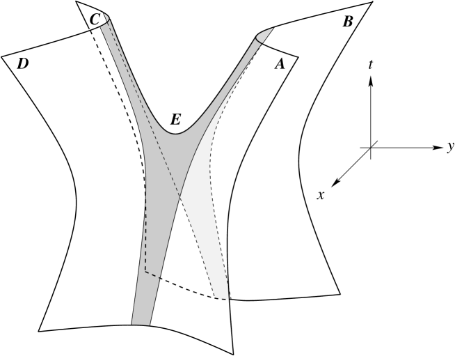
Figure 2: Generalised Scherk Braneworld. (The $(z,w)$ coordinates are suppressed.) In the grey region $E$, the brane metric becomes Riemannian. The boundaries between the Riemannian region and the four Lorentzian regions are null-like, and there the intrinsic curvature diverges. The embedding is, however, smooth across the singularities.

Let us see the causal structure of this brane. The null geodesics with respect to the brane metric obey

$$\left({dy\over dx}\right)_{\pm}=\frac{\cosh y}{\cosh x}\left\{-\sinh x\sinh y\pm\sqrt{\sinh^{2}x\sinh^{2}y-1}\right\}.$$ (58)

One can observe that the light cone becomes thinner and thinner as the boundary surface is approached (See Figure 3,  4). Since the boundary surface is specified as $\sinh x\sinh y=\pm 1$, it follows that $(dx/\cosh x\pm dy/\cosh y)_{boundary}=0$. It then turns out that the induced metric on the boundary surface is degenerate. Indeed, it can be checked that

$$\left({dy\over dx}\right)_{\pm}\left({dy\over dx}\right)^{-1}_{boundary}=1,$$ (59)

and thus the boundary surface is tangent to the light cone. Any causal curves with respect to the brane metric therefore cannot hit the corresponding boundary surface, $\partial A$, $\partial B$, $\partial C$, $\partial D$. Thus, from the view point of the brane causal structure, one might think of the boundary as the “spacelike infinity $i^{0}$”. However, the big difference from the conventional notion of the spacelike infinity is that, it is at a “finite” location in spacelike geodesic distance, and that it is a curvature singularity; the scalar curvature with respect to the brane metric,

$$R=-2\frac{\cosh^{2}x\cosh^{2}y}{(1-\sinh^{2}x\sinh^{2}y)^{2}},$$ (60)

diverges there.

In the asymptotic region $x,y\rightarrow\pm\infty$, the coordinates $x$ and $y$ look like null coordinate, and the brane metric becomes flat. Thus, we have four disconnected Rindler-wedge-like $4$-dimensional universes as in Figure 5.

From the bulk view point, the worldsheet of the brane is connected and everywhere smooth even at $\partial E$. The four regions $A$, $B$, $C$, $D$ are connected via $\partial E$.

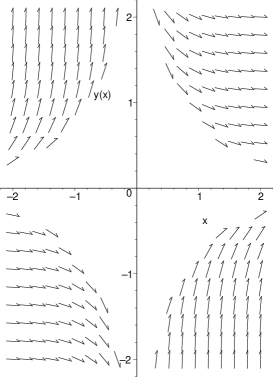
Figure 3: Field of null geodesic tangent “$+$” projected on $(x,y)$-plane.

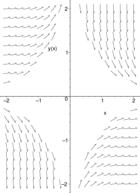
Figure 4: Field of null geodesic tangent “$-$” projected on $(x,y)$-plane.

Figure 5: The causal structure of each Lorentzian region with respect to the brane metric. The $(z,w)$ coordinates are suppressed. ${\mathscr{I}}^{\pm}$, $i^{\pm}$, and $i^{0}$ denote the infinities of the conventional meaning. For example, in the region $A$, $x=+\infty$ at ${\mathscr{I}}^{+}$ and $y=+\infty$ at ${\mathscr{I}}^{-}$, and in the region $B$, $x=-\infty$ at ${\mathscr{I}}^{+}$ and $y=+\infty$ at ${\mathscr{I}}^{-}$. $\partial E$ is the curvature singularity where spacelike geodesics can reach within finite distance. From the bulk view point, the four copies, $A$, $B$, $C$, and $D$ of this panel are smoothly connected via $\partial E$.

The region $E$ of the positive definite metric has a finite total area

$$A=\int_{E}{dx\over\cosh x}{dy\over\cosh y}\sqrt{1-\sinh^{2}x\sinh^{2}y}<\int^{\infty}_{-\infty}{dx\over\cosh x}\int^{\infty}_{-\infty}{dy\over\cosh y}={\pi^{2}\over 4}.$$ (61)

One may also find that the entire $x$ and $y$ axes, which lie entirely within the spacelike region $E$ have finite total length. One may map $x,y\in{{R}}^{2}$ into a square of side $\pi$ by introducing coordinates $X,Y\in(-\pi/2,\pi/2)\times(-\pi/2,\pi/2)$ defined by

$$\sinh x={1\over\tan X},\qquad\sinh y={1\over\tan Y}.$$ (62)

In these coordinates the metric is

$$ds^{2}=dX^{2}+dY^{2}+2{dXdY\over\tan X\tan Y}+dz^{2}+dw^{2}.$$ (63)

The $X$ and $Y$ axes correspond to infinity and the opposites sides of the square, which correspond to the $x$ and $y$ axes, must be identified. The spacelike region is now the exterior of the curve

$$\tan^{2}X\tan^{2}Y=1.$$ (64)

Intrinsically, $E$ is a compact region and the contribution it makes to the action (1) is of course pure-imaginary but nevertheless a finite multiple of the integral over the remaining spatial coordinates $z$ and $w$

$$\pm iAT_{3}\int dzdw.$$ (65)

If we were thinking of a string rather than a 3-brane, the contribution of $E$ to the imaginary part of the action would be finite.

Existence theorems for analogues of Scherk’s singly periodic minimal $2$-surface in ${{E}}^{3}$ have been given for $(n-1)$-ly periodic minimal $n$-surfaces in ${{E}}^{n+1}$ in Ref. [38]. Unfortunately no explicit solutions appears to be known and we are therefore unable to use it to perform a Wick rotation.

4.2 Bulk Field Theory Viewpoint

In fact one can model the process of cosmic string commutation using not the Nambu-Goto action but a classical field theory of Nielsen-Olesen type, in other words using the abelian Higgs model with abelian gauge field $A_{\mu}$ and complex scalar field $\phi$. There is a static vortex solution, in which one identifies the location of the vortex or string with the zero of the Higgs field $\phi(x)=0$. In the time dependent case it has been shown numerically the commutation takes place [39]. During this process one may attempt to identify the position of the moving string with the zero of the Higgs. However the resulting world sheet does not and cannot remain timelike. Judged by the zero, one would have to say that portions of the string travel faster than light. However the energy momentum tensor of the abelian Higgs model satisfies the dominant energy condition. The energy momentum vector and hence the flow of energy is timelike in all frames. It follows from this observation that the zero of the Higgs does not in general track the distribution of energy any more faithfully than does the intersection of two almost parallel searchlight beams track the distribution of photon energy.

What one is seeing therefore is a breakdown of the distinction between bulk and brane. In our minimal surface model, the best that we can is to mimic the very complicated dynamics of the bulk fields by introducing a Riemannian intermediate region. However it should not be endowed with any deep significance. It is merely a sop to compensate for our loss. As Minkowski might well have said, four dimensional spacetime shall be no more, from now on all that remains is the higher dimensional bulk spacetime.

4.3 More Examples of Scherk Braneworlds

Signature changing braneworlds discussed above can be embedded into some curved target space. Simple examples are given by considering a conformally flat bulk with the metric

$$g_{\mu\nu}dX^{\mu}dX^{\nu}=e^{2\lambda}(-dt^{2}+du^{a}du^{a}),$$ (66)

where $\lambda$ is a function of $X^{\mu}$. Then, taking the Monge-gauge, $X^{0}=t(u^{a})$, $X^{a}=u^{a}$ with $a=1,\cdots n=p+1$, one can express the equation of motion (2) as

$$\left\{1-(\partial_{a}t)\partial_{a}t\right\}\left[\partial^{2}_{b}t+n(\partial_{b}t)\partial_{b}\lambda+n\left\{1-(\partial_{a}t)\partial_{a}t\right\}\partial_{t}\lambda\right]+(\partial_{a}t)(\partial_{b}t)\partial_{a}\partial_{b}t=0.$$ (67)

One can find (55) again a solution to the above equation of motion, if $\lambda$ is independent of $X^{0},\,X^{1},\,X^{2}$. The induced metric is given by $e^{2\lambda}$ times the metric (57). In particular, when $\lambda=-\log z$, it describes a Scherk braneworld in anti-de Sitter space.

If one takes a spacelike height function, then one can obtain another variant of the solution (55). Consider bulk metric (66) with $-dt^{2}$ replaced by $d\chi^{2}$ and $du^{a}du^{a}$ by the Minkowski metric $\eta_{ab}du^{a}du^{b}$. With the gauge choice $X^{a}=u^{a}$, $a=0,1,\cdots,p$ and $X^{p+1}=\chi(u^{a})$, one has the equation of motion

$$\left[1+\eta^{cd}(\partial_{c}\chi)\partial_{d}\chi\right]\left[\eta^{ab}\{\partial_{a}\partial_{b}\chi-n(\partial_{a}\chi)\partial_{b}\lambda\}+n\left\{1+\eta^{cd}(\partial_{c}\chi)\partial_{d}\chi\right\}\partial_{\chi}\lambda\right]$$

$$-\eta^{ab}\eta^{cd}(\partial_{a}\chi)(\partial_{d}\chi)\partial_{b}\partial_{c}\chi=0.$$ (68)

If $\lambda$ does not depend on $t,\,y,\,\chi$, one can find a solution

$$\chi=\log(\sinh t)-\log(\sin y),$$ (69)

which is analogous to (55). The corresponding brane metric (for $p=3$) is

$$ds^{2}=e^{2\lambda}\left(\frac{dt^{2}}{\sinh^{2}t}+\frac{dy^{2}}{\sin^{2}y}-2\frac{\cosh t\cos y}{\sinh t\sin y}dtdy+dz^{2}+dw^{2}\right),$$ (70)

where we have set $u^{0}=t$, $u^{1}=y$, $u^{2}=z$, $u^{3}=w$. Inspecting the determinant of this metric, one see that the signature change takes place at $\cosh^{2}t\cos^{2}y=1$.

The world volume geometry is shown in Figure 6, which may be seen as a Lorentzian braneworld (at positive $x$) originated from Euclidean region (at negative $x$).

In terms of $(x,y)$, the null geodesic equation is written by

$$\left({dy\over dx}\right)_{\pm}={e^{x}\sin y\cos y\pm\sqrt{e^{2x}\sin^{2}y\cos^{2}y-1+e^{2x}-2e^{2x}\sin^{2}y}\over 1-e^{2x}+2e^{2x}\sin^{2}y}.$$ (71)

The light cones can be observed from Figures 7, and 8, showing that the light cones become tangent to the boundary between Lorentzian and Euclidean regions.

One can also find a similar solution, $\chi=\log(\sinh t)-\log(\sin y)$. However, this solution does not describe signature change.

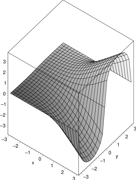
Figure 6: A variant of Scherk braneworld, obtained by using a spacelike height function. (The $(z,w)$ coordinates are suppressed.) This solution also describes a signature changing braneworld (Riemannian region in $x<0$ and Lorentzian regions in $x>0$).

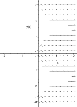
Figure 7: Field of null geodesic tangent “$+$” projected on $(x,y)$-plane. Most regions in $x<0$ are Euclidean.

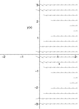
Figure 8: Field of null geodesic tangent “$-$” projected on $(x,y)$-plane.

4.4 Generalised Helicoids

Another possible sources of interesting examples might come from Lorentzian version of the generalised helicoids considered by [40]. These are $p+1$ dimensional submanifolds $\Sigma_{p+1}$ invariant under a $p$-dimensional translation group ${{R}}^{p}$. Such submanifolds are said to be ‘ruled’ and the orbits of the translation group ${{R}}^{p}$ are flat $p$-planes in the ambient flat spacetime. The submanifold $\Sigma_{p+1}$ may be thought of as a one parameter family of $p$-planes. A particularly intriguing case may be obtained from the work of section (1.6) of [40]. Let $x(\tau)$ be a timelike curve $\gamma$ in ${{E}}^{5,1}$, where $\tau$ is propertime along the curve $\gamma$. Let ${\bf e}_{a}$, $a=0,1,\dots,5$ be a pseudo-orthonormal Frenet frame along the curve $\gamma$, so that ${\bf e}_{0}$ is the unit timelike tangent vector to the curve and ${\bf e}_{i}$, $i=1,\dots,5$ are spacelike and

$${d{\bf e}_{a}\over d\tau}=\omega_{a}\thinspace{}^{b}(\tau){\bf e}_{b},$$ (72)

where $\omega_{a}\thinspace^{c}(\tau)\eta_{cb}$ is a skew-symmetric matrix.

Now consider the immersion:

$${\bf X}({u^{0}}=\tau,u^{1},u^{2},u^{3})={\bf x}(\tau)+u^{1}{\bf e}(\tau)_{1}+u^{2}{\bf e}(\tau)_{3}+u^{3}{\bf e}(\tau)_{5},$$ (73)

and $d{{\bf x}(\tau)}/d\tau={\bf e}_{0}$. A simple case is given by

$$\omega_{01}=-k_{0},\quad\omega_{12}=k_{1},\quad\omega_{23}=k_{2},\quad\omega_{34}=k_{3},\quad\omega_{45}=k_{4},\quad\omega_{50}=k_{5}.$$ (74)

The immersion (73) then satisfies the equation of motion (2) for arbitrary constants $k_{a}$. The induced metric, $h_{ab}$, takes the static form,

$$ds^{2} = -\left[(1-k_{0}x-k_{5}z)^{2}-(k_{1}x-k_{2}y)^{2}-(k_{3}y-k_{4}z)^{2}\right]d\tau^{2}$$ (75)

$${}+dx^{2}+dy^{2}+dz^{2},$$

where we have set $u^{1}=x,\,u^{2}=y,\,u^{3}=z$. Note that for $k_{0}\neq 0$, $k_{i}=0$, the above metric describes just a flat plane in the Rindler coordinates (with the replacement $1-k_{0}x\rightarrow k_{0}x$).

When $k_{0}=\beta\neq 0$, $k_{2}=\omega$, $k_{1,3,4,5}=0$, with appropriate choice of ${\bf e}_{a}$, one can express the immersion as

$$X = \left(x-\frac{1}{\beta}\right)\left[-\sinh\beta\tau\frac{\partial}{\partial X^{0}}+\cosh\beta\tau\frac{\partial}{\partial X^{1}}\right]$$ (76)

$${}+y\left[-\sin\omega\tau\frac{\partial}{\partial X^{2}}+\cos\omega\tau\frac{\partial}{\partial X^{3}}\right]+z\frac{\partial}{\partial X^{5}}.$$

Since $h_{\tau\tau}=\omega^{2}y^{2}-(1-\beta x)^{2}$, the induced metric changes its signature at $\omega y=\pm(1-\beta x)$. The Jacobi-matrix is of rank 4 at the points of signature change, except the point $x=1/\beta$ and $y=0$, hence the immersion itself is regular there. However, the intrinsic curvature,

$$R=\frac{2}{(h_{\tau\tau})^{2}}[\beta^{4}+\omega^{4}+(\beta^{2}+\omega^{2})h_{\tau\tau}],$$ (77)

of the induced metric diverges there. The signature change therefore looks again an occurrence of a curvature singularity from the view point of residents on this helicoid, as in the Scherk braneworld case.

5 Discussion

We have provided models of the braneworlds that admit topology change and signature change in a smooth Lorentzian bulk. We also gave models of oscillating and spinning brane universes by generalising Lorentzian catenoid and helicoid. Our braneworld models obey the Dirac-Born-Infeld equations of motion, but their self-gravity was neglected so as to allow a simple model.

Concerning the signature changing brane models, we should point out that although there are certain similarities with the minimal surfaces we have used in this paper and certain instantons, i.e. complex saddle points used to describe the high energy limit of string scattering [41, 42, 43, 44] which were extended to include the presence of D-branes in [45] there are important differences. Firstly we have in mind not only strings, i.e., $p=1$ but the case of general $p$-branes, $p>1$. Indeed for us the most interesting case is $p=3$. Secondly, our solutions are real, where as those used in [41, 42, 43, 44] are pure imaginary although the induced metric is always real but positive definite. It is possible in some cases, for example, that some forms of Scherks’ surface may be related by analytic continuation to those used in [41, 42, 43, 44, 45]. However, the scattering processes we have had in mind are, at least from the bulk point of view, entirely classical. As we have speculated above, it may be that from the world volume point of view they may be thought of in a more quantum mechanical way. If so, the differences in our approach and that of [41, 42, 43, 44, 45] may not be so great as at first appears. It would clearly be of great interest to pursue this connection further. A treatment of intersecting $D$-branes in relation to tachyon condensation is given in Ref. [46].

In our examples, the boundary between the Lorentzian and Euclidean regions corresponds to a curvature singularity with respect to the induced metric of a signature changing braneworld. In order for inhabitants on the brane to understand the situation, they need to develop quantum gravity theory in 4-dimensions. On the other hand, from the bulk view point, the brane is everywhere, even at the points corresponding to the singularity, smooth. It can be simply described by embedding equation. This observation suggests an possible way of resolving spacetime singularities in the braneworld context. This also conforms to the spirit of holographic principle or bulk-boundary correspondence, in the sense that quantum theory on a brane could be understood in terms of bulk classical theory. In order to make spacetime metric real, the Euclidean approach needs the existence of a totally geodesic spacelike hypersurface. This is one of great limitations of the uses of the Euclidean approach. In the present model, the Euclidean region of a braneworld is connected with Lorentzian region at spacelike surfaces which are not totally geodesic surface but correspond to a singularity. It would be interesting if one can develop Euclidean Quantum Gravity by implementing the signature change of a braneworld in a smooth Lorentzian bulk spacetime.

Acknowledgements

GWG would like to thank Costas Bachas, Michael Green, Ergin Sezgin and Andrew Strominger for helpful discussions and encouragement. In particular, conversations with Costas Bachas at ENS in Paris during late 1999 were extremely illuminating. A preliminary version of this work was described at the George and Cynthia Mitchell Institute for Fundamental Physics in Spring 2002. We also wish to thank Koji Hashimoto, Jose Senovilla, Paul Shellard and Supriya Kar. This research was supported in part by the Japan Society for the Promotion of Science.

References

- [1] L. Randall and R. Sundrum, Phys. Rev. Lett. 83, 4690 (1999).
- [2] W. Rouse Ball, A Hypothesis relating to the Nature of the Ether Gravity, Messenger of Mathematics 21, 20–24 (1891).
- [3] D.W. Joseph, Phys. Rev. 126, 319 (1962).
- [4] A. Friedman, Rev. Mod. Phys. 37, 201 (1965).
- [5] J. Rosen, Rev. Mod. Phys. 37, 204 (1965).
- [6] R. Penrose, Rev. Mod. Phys. 37, 215 (1965).
- [7] H.F. Goenner, in General Relativity and Gravitation, Vol. 1, 441, ed. A. Held (Plenum, New York, 1980)
- [8] S. Deser, F.A.E. Pirani and D.C. Robinson, Phys. Rev. D 14, 3301 (1976).
- [9] K. Akama, Lecture Notes in Phys. 176, 267 (1982) (hep-th/0001113).
- [10] V.A. Rubakov and M.E. Shaposhnikov, Phys. Lett. B 152, 136 (1983).
- [11] M. Visser, Phys. Lett. B 159, 22 (1985).
- [12] G.W. Gibbons and D.L. Wiltshire, Nucl. Phys. B 287 717 (1987).
- [13] J. Khoury, B.A. Ovrut, P.J. Steinhardt, and N. Turok, Phys. Rev. D 64, 123522 (2001).
- [14] R. Kallosh, L. Kofman, A. Linde, Phys. Rev. D64, 123523 (2001).
- [15] P.J. Steinhardt, and N. Turok, Science 296, 1436 (2002).
- [16] R.P. Geroch, J. Math. Phys. 8, 782 (1967).
- [17] F.J. Tipler, Phys. Lett. B 165, 67 (1985).
- [18] R. Gregory and A. Padilla, Class. Quantum Grav. 19, 279 (2002).
- [19] W.B. Perkins, Phys. Lett. B 504, 28 (2001).
- [20] M. Bucher, Phys. Lett. B 530, 1 (2002).
- [21] U. Gen, A. Ishibashi, and T. Tanaka, Phys. Rev. D 66, 023519 (2002).
- [22] S. Kanno, M. Sasaki, and J. Soda, Prog. Theor. Phys. 109, 357 (2003).
- [23] M. Mars, J.M.M. Senovilla, and R. Vera, Phys. Rev. Lett. 86, 4219 (2001).
- [24] K. Hashimoto, P.-M. Ho, and J.E. Wang, Phys. Rev. Lett. 90, 141601 (2003).
- [25] K. Hashimoto, P.-M. Ho, S. Nagaoka, and J.E. Wang, Phys. Rev. D 68, 026007 (2003).
- [26] G.W. Gibbons and C.A.R. Herdeiro, Phys. Rev. D 63, 064006 (2001).
- [27] S. Kar and S. Panda, JHEP 0211, 052 (2002).
- [28] G. Monge, Application de l’analyse à la geometrie (1807): reprinted as X les cours historiques de l’École Polytechnique ISBN2-7298-9440-3, ellips (1994).
- [29] R.D. Kamien and T.C. Lubensky, Phys. Rev. Lett. 82, 2892 (1999).
- [30] R.D. Kamien, Appl. Math. Lett. 14, 797 (2001).
- [31] J.C.C. Nitsche, Lectures on minimal surfaces Vol. 1, Cambridge Univ. Press (1989).
- [32] H. Alencar, Trans. American Math. Soc., 337, 129 (1993).
- [33] R Osserman, A Survey of Minimal Surfaces, Dover
- [34] K. Kikkawa and M. Yamasaki, Prog. Theor. Phys. 76, 379 (1988).
- [35] J. Hoppe and H. Nicolai, Phys. Lett. B 196, 451 (1987).
- [36] B. Neilsen, J. Geometry Phys 4, 1 (1987).
- [37] G.W. Gibbons, Nucl. Phys. B 514, 603 (1998).
- [38] F. Pacard, math.DG/0109131.
- [39] E.P.S. Shellard, Nucl. Phys. B 283, 624 (1987).
- [40] J.L. Barbosa and M. Do Carmo, An. Acad. brasil. Cienc., 53, 403 (1981).
- [41] D.J. Gross, Phys. Rev. Lett. 60, 1229 (1988).
- [42] D.J. Gross, Phil. Trans. R. Soc. Lond. A 329, 401 (1989).
- [43] D.J. Gross and P.F. Mende, Phys. Lett. B197, 129 (1987).
- [44] D.J. Gross and P.F. Mende, Nucl. Phys. B 303, 407 (1988).
- [45] C. Bachas and B. Pioline, JHEP 9912 004, (1999).
- [46] K. Hashimoto and S. Nagaoka, JHEP 0306 034, (2003).