UV Perturbations in Brane Gas Cosmology

Abstract

We consider the effect of the ultraviolet (UV) or short wavelength modes on the background of Brane Gas Cosmology. We find that the string matter sources are negligible in the UV and that the evolution is given primarily by the dilaton perturbation. We also find that the linear perturbations are well behaved and the predictions of Brane Gas Cosmology are robust against the introduction of linear perturbations. In particular, we find that the stabilization of the extra dimensions (moduli) remains valid in the presence of dilaton and string perturbations.

I Introduction

Understanding the behavior of strings in a time dependent background has been a subject of much interest and has been pursued in a number of differing ways. One scenario, known as Brane Gas Cosmology (BGC), is devoted to understanding the effect that string and brane gases could have on a dilaton-gravity background in the early Universe bv ; vafa ; bgc ; isotropization ; stable ; extended . In bv , it was suggested that the energy associated with the winding of strings around the compact dimensions would produce a confining potential for the scale factor and halt the cosmological expansion. The analysis of BGC was initially performed under the assumption of a homogeneous and isotropic cosmology. The results were recently extended to the case of anisotropic cosmology in isotropization . There, it was shown that string gases can give rise to three dimensions growing large and isotropic due to string annihilation while the other six dimensions remain confined. In stable it was shown that by considering both momentum and winding modes of strings, the six confined dimensions can be stabilized at the self-dual radius, where the energy of the string gas is minimal. This result demonstrated that, in BGC, the volume moduli of the extra dimensions can be stabilized in a natural and intuitive way.

In recent work perturbations , we considered the effect of string inhomogeneities and dilaton fluctuations on BGC. The string sources of BGC are usually represented by a perfect fluid with homogeneous energy and pressure densities given by the mass spectrum of the strings (see e.g. bgc ; stable ; subodh ). One may worry that inhomogeneities of string sources (in particular strings winding around the confined dimensions) as a function of the unconfined spatial directions could lead to serious instabilities which could ruin the main successes of BGC, namely the prediction that three directions become large leaving the other six confined uniformly as a function of the coordinates of the large spatial sections. In perturbations , we found that at the linear level BGC is robust with respect to long wavelength perturbations. In that paper it was found that at late times the inhomogeneities are subleading compared to the evolution of the background. In this paper we will extend our considerations to the ultraviolet or small wavelength perturbations. Our expectation was that on small wavelengths, the motion of the strings would smear out potential instabilities in a way analogous to how the motion of light particles (“free-streaming”) leads to a decay of short wavelength fluctuations in standard cosmology (see e.g. Peebles for a review). However, we will find that the string matter perturbations are actually sub-leading in the evolution and the dilaton perturbation is the primary driving force of instability.

For reference, in Section 2 and 3 we present the background solution and perturbed equations as found in perturbations . The crucial new results appear in Section 4, where we derive the perturbation equations for the UV modes and then solve for their late time behavior. The full equations are presented in the Appendix. We conclude with a discussion of our findings and future prospects in Section 5.

II Background Solution

Our starting point is the low energy effective action for the bulk space-time with string matter sources vafa ,

$$S=\frac{1}{4\pi\alpha^{\prime}}\int d^{D}x\sqrt{-g}e^{-2\varphi}\Bigl{(}R+4(\nabla\varphi)^{2}-\frac{1}{12}H^{2}\Bigr{)}+S_{\text{m}}\,,$$ (1)

where $R$ denotes the Ricci scalar, $g$ is the determinant of the background metric, $\varphi$ is the dilaton field, and $H$ is the field strength of an antisymmetric tensor field. The action of the matter sources is denoted by $S_{\text{m}}$. For example, with $D=10$ this is the low energy effective action of type II-A superstring theory. For the purposes of this paper we will ignore the effects of branes, since it will be the winding and momentum modes of the string that ultimately determine the dimensionality and stability of space-time bgc . Here, we will ignore the effects of fluxes , i.e. we set $H=0$.

This action yields the following equations of motion,

$$R_{\mu}^{\;\;\nu}+2\nabla_{\mu}\nabla^{\nu}\varphi=8\pi M^{-2}_{p}\;e^{2\varphi}T_{\mu}^{\;\;\nu},$$

$$R+4\nabla_{\kappa}\nabla^{\kappa}\varphi-4\nabla_{\kappa}\varphi\nabla^{\kappa}\varphi=0,$$ (2)

where $\nabla$ is the covariant derivative.

We will work in the conformal frame with a homogeneous metric of the form

$$ds^{2}=e^{2\lambda(\eta)}\Bigl{(}d\eta^{2}-\delta_{ij}dx^{i}dx^{j}\Bigr{)}-e^{2\nu(\eta)}\delta_{mn}dx^{m}dx^{n},$$ (3)

where $(\eta,x^{i})$ are the coordinates of $3+1$ space-time and $x^{m}$ are the coordinates of the other six dimensions, all of which can be taken to be isotropic isotropization . The scale factors $a(\eta)$ and $b(\eta)$ are given by $\lambda\equiv\ln(a)$ and $\nu\equiv\ln(b)$.

We consider the effect of the strings on the background through their stress energy tensor

$$T_{\mu}^{\>\>\nu}\equiv diag(\rho,-p_{i},-p_{m}),$$ (4)

where $\rho$ is the energy density of the strings, $p_{i}$ ($i=1\ldots 3$) is the pressure in the expanding dimensions and $p_{m}$ ($m=4\ldots 9$) is the pressure in the small dimensions (because of our assumption of isotropy of each subspace, there is only one independent $p_{i}$ and one independent $p_{m}$).

Strings contain winding modes, momentum modes and oscillatory modes. However, since the energies of the oscillatory modes are independent of the size of the dimensions, and since the winding modes and momentum modes dominate the thermodynamic partition function at very small and very large radii of the spatial dimensions, here we shall neglect the oscillatory modes. In the absence of string interactions, the contributions to the stress tensor coming from the string winding modes and momentum modes ($T^{\text{w}}_{\mu\nu}$ and $T^{\text{m}}_{\mu\nu}$ respectively) are separately conserved,

$$T_{\mu\nu}=T^{\text{w}}_{\mu\nu}+T^{\text{m}}_{\mu\nu}$$

$$\nabla^{\mu}T^{\text{w}}_{\mu\nu}=0,\;\;\;\;\;\;\nabla^{\mu}T^{\text{m}}_{\mu\nu}=0\,.$$ (5)

The conservation equations take the form

$$\rho^{\prime\>{\text{w},m}}+\sum_{i=1}^{9}\lambda_{i}^{\prime}(\rho^{\text{w},m}-p^{\text{w},m}_{i})=0,$$ (6)

where the derivatives are with respect to the conformal time $\eta$, and where for the moment we consider 9 independent scale factors.

Expressing (II) in terms of the metric (3) and the stress tensor (4), we find the following system of equations,

$$-3\lambda^{\prime\prime}-6\nu^{\prime\prime}+6\lambda^{\prime}\nu^{\prime}-6\nu^{\prime 2}+\varphi^{\prime\prime}-\lambda^{\prime}\varphi^{\prime}=8\pi M_{p}^{-2}e^{\varphi+2\lambda}\rho,$$ (7)

$$-\lambda^{\prime\prime}+2\lambda^{\prime 2}+6\lambda^{\prime}\nu^{\prime}+\lambda^{\prime}\varphi^{\prime}=-8\pi M_{p}^{-2}e^{\varphi+2\lambda}p_{i},$$ (8)

$$-\nu^{\prime\prime}+6\nu^{\prime 2}+2\lambda^{\prime}\nu^{\prime}+\varphi^{\prime}\nu^{\prime}=-8\pi M_{p}^{-2}e^{\varphi+2\lambda}p_{m},$$ (9)

$$-6\lambda^{\prime\prime}-12\nu^{\prime\prime}-24\lambda^{\prime}\nu^{\prime}-42\nu^{\prime 2}-6\lambda^{\prime 2}-\varphi^{\prime 2}+2\varphi^{\prime\prime}+8\lambda^{\prime}\varphi^{\prime}+12\varphi^{\prime}\nu^{\prime}=0.$$ (10)

The explicit forms of the energy density and pressure were given in stable ,

$$\rho=3\mu N^{(3)}e^{-2\lambda-6\nu}+3\mu M^{(3)}e^{-4\lambda-6\nu}+6\mu N^{(6)}e^{-3\lambda-5\nu}+6\mu M^{(6)}e^{-3\lambda-7\nu},$$ (11)

$$p_{i}=-\mu N^{(3)}e^{-2\lambda-6\nu}+\mu M^{(3)}e^{-4\lambda-6\nu},$$ (12)

$$p_{m}=-\mu N^{(6)}e^{-3\lambda-5\nu}+\mu M^{(6)}e^{-3\lambda-7\nu},$$ (13)

where $\mu$ is a constant, $N^{(3)}$ and $M^{(3)}$ are the numbers of winding and momentum modes in the large directions, and $N^{(6)}$ and $M^{(6)}$ in the six small directions.

We are interested in solutions that stabilize the internal dimensions, while allowing the three large dimensions to expand. Such solutions were discussed in stable , where it was shown that the winding and momentum modes of the strings lead naturally to stable compactifications of the internal dimensions at the self dual radius. This remains true as the other three dimensions grow large, which is possible because the string gas can maintain thermal equilibrium in three dimensions and the string winding modes are able to annihilate. Thus, we will set $N^{(3)}=0$. At the self dual radius, the number of winding modes is equal to the number of momentum modes (i.e. $N^{(6)}=M^{(6)}$) and the pressure vanishes ($p_{m}=0$).

In Ref. stable , the solutions subject to the above conditions on the winding and momentum numbers were found numerically. In this paper, we wish to study the stability of these solutions towards linear perturbations in the time interval when the internal dimensions have stabilized and the large dimensions give power law expansion. In the following section, we will derive the equations for the linear fluctuations. The coefficients in these equations depend on the background solution. We will use analytical expressions which approximate the numerically obtained solutions of stable . We restrict our initial conditions so that the evolution preserves the low energy and small string coupling assumptions ($g_{s}\sim e^{2\varphi}\ll 1$).

We can approximate a typical solution of the equations (7-10) by

$$\lambda(\eta)=k_{1}\ln(\eta)+\lambda_{0}\;\;\;{\text{o}r}\;\;\;a(\eta)=a_{0}\eta^{k_{1}},$$

$$\varphi(\eta)=-k_{2}\ln(\eta)+\varphi_{0},$$ (14)

where the constants $k_{1}$, $k_{2}$, $\lambda_{0}$ and $\varphi_{0}$ depend on the choice of initial conditions. We have made use of $\nu=\nu^{\prime}=\nu^{\prime\prime}=0$, $N^{(3)}=0$, $N^{(6)}=M^{(6)}$, $p_{m}=0$. Note that in this limit (9) is trivially satisfied. An example of a solution yielding stabilized dimensions and three dimensions growing large corresponds to $k_{1}=\frac{1}{9}$ and $k_{2}=\frac{9}{7}$. The numerical solution of stable and the analytical approximation used in this paper are compared in Fig. 1, for the above values of the constants $k_{1}$ and $k_{2}$.

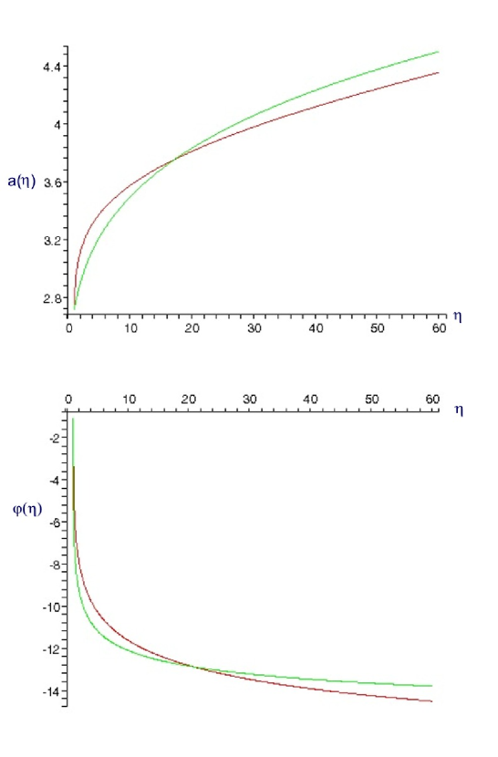
Figure 1: A comparison between the numerical background solutions obtained in stable (red or light line) and the analytical approximation used in this paper (green or dark line).

III Scalar Metric Perturbations

In this section we consider the growth of scalar metric perturbations (see e.g. MFB for a comprehensive review of the theory of cosmological perturbations) due to the presence of string inhomogeneities. We are interested in the case where the fluctuations depend only on the external coordinates and conformal time, not on the coordinates of the internal dimensions. For simplicity we work in the generalized longitudinal gauge in which the metric perturbations are only in the diagonal metric elements . Thus, the metric including linear fluctuations is given by

$$ds^{2}=e^{2\lambda(\eta)}\Bigl{(}(1+2\phi)d\eta^{2}-(1-2\psi)\delta_{ij}dx^{i}dx^{j}\Bigr{)}-e^{2\nu(\eta)}(1-2\xi)\delta_{mn}dx^{m}dx^{n}.$$ (15)

The dilaton $\varphi$ also fluctuates about its background value $\varphi_{0}$. The dilaton fluctuation $\chi$ is determined by

$$\varphi=\varphi_{0}+\delta\varphi,\;\;\;\;\;\;\chi\equiv\delta\varphi.$$ (16)

In the above, the fluctuating fields $\chi,\phi,\psi$ and $\xi$ are functions of the external coordinates $x^{i}$ and time, i.e.

$$\chi=\chi(\eta,x^{i}),\>\>\>\>\phi=\phi(\eta,x^{i}),\>\>\>\>\psi=\psi(\eta,x^{i}),\>\>\>\>\xi=\xi(\eta,x^{i}).$$ (17)

The perturbations of the matter energy momentum tensor result from over-densities and under-densities in the number of strings. From (11)-(13) and noting that we are interested in the case when $N^{(3)}=0$ and $M^{(6)}=N^{(6)}$ we find,

$$\delta\rho=\delta\rho_{{\text{w}}}+\delta\rho_{{\text{m}}},$$ (18)

$$\delta\rho_{{\text{w}}}=30\mu N\xi e^{-3\lambda}+18\mu N\psi e^{-3\lambda}+6\delta N^{(6)}e^{-3\lambda},$$ (19)

$$\delta\rho_{{\text{m}}}=42\mu N\xi e^{-3\lambda}+18\mu M\xi e^{-4\lambda}+18\mu N\psi e^{-3\lambda}+12\mu M\psi e^{-4\lambda}+6\mu\delta M^{(6)}e^{-3\lambda}+$$ (20)

$$+3\mu\delta Me^{-4\lambda},$$ (21)

$$\delta p_{\lambda}=6\mu M\xi e^{-4\lambda}+4\mu M\psi e^{-4\lambda}+\mu\delta Me^{-4\lambda},$$ (22)

$$\delta p_{\nu}=2\mu N\xi e^{-3\lambda}-\mu\delta N^{(6)}e^{-3\lambda}+\mu\delta M^{(6)}e^{-3\lambda},$$ (23)

where we define $N\equiv N^{(6)}=M^{(6)}$ and $M\equiv M^{(3)}$. The fluctuations $\delta N^{(6)}$, $\delta M^{(6)}$, and $\delta M$ are taken as functions of both conformal time and the external space, e.g. $\delta N^{(6)}=\delta N(\eta,x^{i})$.

It follows from (6) that the perturbed sources obey modified conservation equations for both the winding and momentum modes,

$$\delta\rho^{\prime\>{\text{w},m}}+\sum_{i=1}^{9}\lambda_{i}^{\prime}(\delta\rho^{\text{w},m}-\delta p^{\text{w},m}_{i})+\sum_{i=1}^{9}\delta\lambda_{i}^{\prime}(\rho^{\text{w},m}-p^{\text{w},m}_{i})=0,$$ (24)

where $\delta\lambda=a^{-1}\delta a=-\psi$ and $\delta\nu=b^{-1}\delta b=-\xi$ are spatial variations.

We rewrite (II) to take the more familiar form of the Einstein and dilaton equations, namely

$$R_{\mu}^{\nu}-\frac{1}{2}\delta_{\mu}^{\nu}R=e^{2\varphi}T_{\mu}^{\nu}-2g^{\alpha\nu}\nabla_{\mu}\nabla_{\alpha}\varphi+2\delta_{\mu}^{\nu}\Bigl{(}g^{\mu\nu}\nabla_{\mu}\nabla_{\nu}\varphi-g^{\mu\nu}\partial_{\mu}\varphi\partial_{\nu}\varphi\Bigr{)},$$

$$g^{\mu\nu}\partial_{\mu}\varphi\partial_{\nu}\varphi-\frac{1}{2}g^{\mu\nu}\nabla_{\mu}\nabla_{\nu}\varphi=\frac{1}{4}e^{2\varphi}T^{\mu}_{\mu},$$ (25)

where we invoke Planckian units (i.e. $8\pi M_{p}^{-2}=1$). Plugging the perturbed metric (15) and dilaton into these equations, making use of the background equations of motion, and linearizing the equations about the background (i.e. keeping only terms linear in the fluctuations) yields the following set of equations:

$${\vec{\nabla}}^{2}\psi+3{\vec{\nabla}}^{2}\xi-9{\cal{H}}\xi^{\prime}-3{\cal{H}}\psi^{\prime}-3{\cal{H}}^{2}\phi=\frac{1}{2}e^{2\varphi+2\lambda}\Bigl{(}2\chi T^{0}_{0}+\delta T^{0}_{0}\Bigr{)}-6{\cal{H}}\phi\varphi^{\prime}$$

$$-3\psi^{\prime}\varphi^{\prime}-6\xi^{\prime}\varphi^{\prime}-{\vec{\nabla}}^{2}\chi+3{\cal{H}}\chi^{\prime}+2\phi\varphi^{\prime 2}-2\chi^{\prime}\varphi^{\prime},$$ (26)

$$\partial_{i}\psi^{\prime}+3\partial_{i}\xi^{\prime}+{\cal{H}}\partial_{i}\phi-3{\cal{H}}\partial_{i}\xi=\frac{1}{2}e^{2\varphi+2\lambda}\delta T_{0}^{i}+\partial_{i}\phi\varphi^{\prime}-\partial_{i}\chi^{\prime}+{\cal{H}}\partial_{i}\chi,$$ (27)

$$\partial_{i}\partial_{j}\Bigl{(}\phi-\psi-6\xi-2\chi\Bigr{)}=0\;\;\;\;\;\;i\neq j,$$ (28)

$$\Bigl{(}\partial_{i}^{2}-\vec{\nabla}^{2}\Bigr{)}\Bigl{(}\phi-\psi-6\xi\Bigr{)}-2\psi^{\prime\prime}-6\xi^{\prime\prime}-4{\cal{H}}\psi^{\prime}-6{\cal{H}}\xi^{\prime}-2{\cal{H}}{{}^{2}}\phi-4{\cal{H}}^{\prime}\phi-2\phi^{\prime}{\cal{H}}$$

$$=e^{2\varphi+2\lambda}\Bigl{(}2\chi T^{i}_{i}+\delta T^{i}_{i}\Bigr{)}+2\partial_{i}^{2}\chi-4\phi\varphi^{\prime\prime}-2\phi^{\prime}\varphi^{\prime}-4{\cal{H}}\phi\varphi^{\prime}-4\psi^{\prime}\phi^{\prime}-12\xi^{\prime}\varphi^{\prime}$$

$$+2\chi^{\prime\prime}-2\vec{\nabla}^{2}\chi+2{\cal{H}}\chi^{\prime}+4\phi\varphi^{\prime 2}-4\chi^{\prime}\varphi^{\prime},$$ (29)

$$-{\vec{\nabla}}^{2}\phi+5{\vec{\nabla}}^{2}\xi-5\xi^{\prime\prime}+2{\vec{\nabla}}^{2}\psi-3\psi^{\prime\prime}-10{\cal{H}}\xi^{\prime}-3\phi^{\prime}{\cal{H}}-9{\cal{H}}\psi^{\prime}-6{\cal{H}}^{2}\phi-6{\cal{H}}^{\prime}\phi$$

$$=e^{2\varphi+2\lambda}\Bigl{(}2\chi T^{m}_{m}+\delta T^{m}_{m}\Bigr{)}-4\phi\varphi^{\prime\prime}-2\phi^{\prime}\varphi^{\prime}-8{\cal{H}}\phi\varphi^{\prime}-6\psi^{\prime}\varphi^{\prime}-10\xi^{\prime}\varphi^{\prime}+2\chi^{\prime\prime}$$

$$-2{\vec{\nabla}}^{2}\chi+4{\cal{H}}\chi^{\prime}+4\phi\varphi^{\prime 2}-4\chi^{\prime}\phi^{\prime},$$ (30)

$$-2\phi\varphi^{\prime 2}+2\varphi^{\prime}\chi^{\prime}+\phi\varphi^{\prime\prime}-6\psi{\cal{H}}\varphi^{\prime}+\frac{1}{2}\phi^{\prime}\varphi^{\prime}-2{\cal{H}}\phi\varphi^{\prime}-\frac{3}{2}\psi^{\prime}\varphi^{\prime}-3\xi^{\prime}\varphi^{\prime}-\frac{1}{2}\chi^{\prime\prime}$$

$$+\frac{1}{2}{\vec{\nabla}}^{2}\chi-{\cal{H}}\chi^{\prime}=\frac{1}{4}e^{2\varphi+2\lambda}\Bigl{(}2\chi T+\delta T\Bigr{)},$$ (31)

where $T\equiv T^{\mu}_{\mu}$ is the trace of the stress tensor and $\vec{\nabla}^{2}\equiv\partial_{x}^{2}+\partial_{y}^{2}+\partial_{z}^{2}$ is the spatial Laplacian. The modified conservation equations (24) take the form

$$\frac{d}{d\eta}\Bigl{(}\delta N^{(6)}\Bigr{)}=7N\xi^{\prime},$$ (32)

$$42\mu N\xi^{\prime}-72\mu M\xi\lambda^{\prime}e^{-\lambda}-48\mu M\psi\lambda^{\prime}e^{-\lambda}+12\mu M\psi^{\prime}e^{-\lambda}+6\mu\frac{d}{d\eta}\Bigl{(}\delta M^{(6)}\Bigr{)}$$

$$-12\mu\delta M\lambda^{\prime}e^{-\lambda}+3\mu\frac{d}{d\eta}\Bigl{(}\delta M\Bigr{)}e^{-\lambda}=0.$$ (33)

These equations give us the evolution of the metric perturbations $\phi$, $\psi$, and $\xi$ in terms of the matter perturbations $\chi$, $\delta\rho$, and $\delta p_{i}$. At first glance, it may appear that the above system is over-determined since we have eight equations for seven unknowns. However, as is the case in standard cosmology, the conservation equations are not independent of the Einstein equations. Thus, we can choose to keep only one of the modified conservation equations and our system will be consistent.

IV Ultraviolet Modes

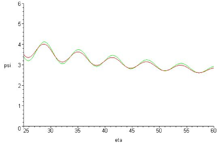
Figure 2: A comparison between the numerical value of the external metric perturbation $\psi$ (red or dark line) and the analytical approximation found in this paper (green or light line).

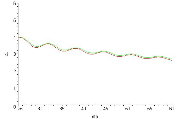
Figure 3: A comparison between the numerical value of the internal metric perturbation $\xi$ (red or dark line) and the analytical approximation found in this paper (green or light line).

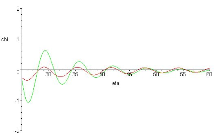
Figure 4: A comparison between the numerical value of the dilaton perturbation $\chi$ (red or dark line) and the analytical approximation found in this paper (green or light line).

We now want to solve the equations (III)-(III) in the limit of small wavelength (or high energy). We can simplify the analysis by working in terms of the Fourier modes, e.g.

$$\psi(\eta,\vec{x})=\sum_{k}\psi_{k}(\eta)e^{i\vec{k}\cdot\vec{x}},\;\;\;\delta N(\eta,\vec{x})=\sum_{k}\delta N_{k}(\eta)e^{i\vec{k}\cdot\vec{x}},\;\;\;{\text{e}tc...}.$$

Note that in the remainder of this paper it will be understood that when we speak of perturbed quantities we are referring to the time dependent Fourier modes, e.g. $\psi\equiv\psi_{k}(\eta)$.

Using (28) to eliminate the scalar metric perturbation $\phi$, the equations (III)-(III) in Fourier space take the form

$$\frac{61}{7\eta}\xi^{\prime}+\frac{61}{21\eta}\chi^{\prime}+\frac{88}{21\eta}\psi^{\prime}+\Biggl{(}\frac{338}{189\eta^{2}}+\vec{k}^{2}\Biggr{)}\chi+\Biggl{(}\frac{338}{63\eta^{2}}+3\vec{k}^{2}\Biggr{)}\xi+\Biggl{(}\frac{169}{189\eta^{2}}+\vec{k}^{2}\Biggr{)}\psi=0,$$ (34)

$$\psi^{\prime}+3\xi^{\prime}+\chi^{\prime}+\frac{88}{63\eta}\psi+\frac{169}{21\eta}\xi+\frac{169}{63\eta}\chi=0$$ (35)

$$2\psi^{\prime\prime}+6\xi^{\prime\prime}+2\chi^{\prime\prime}+\frac{176}{21\eta}\psi^{\prime}+\frac{230}{7\eta}\xi^{\prime}+\frac{230}{21\eta}\chi^{\prime}+\frac{6434}{3969\eta^{2}}\psi+\frac{12868}{1323\eta^{2}}\xi+\frac{12868}{3969\eta^{2}}\chi=0,$$ (36)

$$3\psi^{\prime\prime}+5\xi^{\prime\prime}+2\chi^{\prime\prime}+\frac{244}{21\eta}\psi^{\prime}+\frac{1978}{63\eta}\xi^{\prime}+\frac{718}{63\eta}\chi^{\prime}+\Biggl{(}\frac{2672}{1323\eta^{2}}+\vec{k}^{2}\Biggr{)}\psi+\Biggl{(}\frac{5344}{441\eta^{2}}-\vec{k}^{2}\Biggr{)}\xi+\frac{5344}{1323\eta^{2}}\chi=0,$$ (37)

$$\frac{1}{2}\chi^{\prime\prime}-\frac{9}{7\eta}\psi^{\prime}+\frac{250}{63\eta}\chi^{\prime}+\frac{43}{49\eta^{2}}\psi+\frac{510}{49\eta^{2}}\xi+\Biggl{(}\frac{170}{49\eta^{2}}+\frac{1}{2}\vec{k}^{2}\Biggr{)}\chi=0.$$ (38)

To obtain these equations we have made use of the background solution (14) and dropped all but the leading order terms since we are interested in the late time ($\eta>>1$) and small wavelength ($k>>1$) behavior . In particular, we see that as in the long wavelength case, the source terms $\delta N$, $\delta M_{3}$, and $\delta M_{6}$ are negligible at late times. This is because the string matter sources are sub-leading in the evolution equations and instability is primarily sourced by the dilaton perturbation. This result is crucial to our outcome and is discussed in detail in the Appendix.

We also notice that (34) and (35) are only first order in time derivatives and can be taken as constraints on the initial conditions. This leaves us with the equations of motion (36), (37), and (38). These equations can be put in a more tractable form by introducing the two fields $\Delta$ and $\Theta$,

$$\psi=\Delta+\Theta\;\;\;\;\;\xi=\Delta-\frac{1}{3}\Theta.$$ (39)

The equations can then be written as

$$\frac{1}{2}\chi^{\prime\prime}+\frac{250}{63\eta}\chi^{\prime}+\Biggl{(}\frac{170}{49\eta^{2}}+\frac{1}{2}\vec{k}^{2}\Biggr{)}\chi=\frac{9}{7\eta}\Delta^{\prime}+\frac{9}{7\eta}\Theta^{\prime}-\frac{79}{7\eta^{2}}\Delta+\frac{127}{49\eta^{2}}\Theta$$ (40)

$$\frac{4}{3}\Theta^{\prime\prime}+\frac{704}{189\eta}\Theta^{\prime}+\Biggl{(}\frac{4}{3}\vec{k}^{2}-\frac{226}{567\eta^{2}}\Biggr{)}\Theta=-\frac{16}{9\eta}\Delta^{\prime}-\frac{4}{9\eta}\chi^{\prime}-\frac{226}{81\eta^{2}}\Delta-\frac{452}{567\eta^{2}}\chi$$ (41)

$$8\Delta^{\prime\prime}+\frac{866}{21\eta}\Delta^{\prime}+\frac{6434}{567\eta^{2}}\Delta=-2\chi^{\prime\prime}-\frac{230}{21\eta}\chi^{\prime}+\frac{18}{7\eta}\Theta^{\prime}+\frac{6434}{3969\eta^{2}}\Theta-\frac{12868}{3969\eta^{2}}\chi$$ (42)

where we have written the system as to isolate the second order derivative terms in $\Theta$ and $\Delta$ and again dropped terms that are negligible given $k,\eta>>1$. We first solve (40) for $\chi$, neglecting the right side of the equation and treating it as a negligible source term. This perturbative approach will only be justified if, after solving for $\Delta$ and $\Theta$ in the remaining equations, we return to (40) to make sure these terms remain negligible. Proceeding in this way we find that to first order $\chi$ is given by,

$$\chi_{0}=c_{1}(k)\frac{J_{a}(k\eta)}{(k\eta)^{a}}+c_{2}(k)\frac{Y_{a}(k\eta)}{(k\eta)^{a}},$$ (43)

where the $c_{i}(k)$ are arbitrary constants, $a=\frac{147}{126}$, $J_{a}$ is a Bessel Function of the first kind, and $Y_{a}$ is a Bessel Function of the second kind. We proceed by solving (41) for $\Theta$ using $\chi=\chi_{0}$ and again neglecting the terms that depend on $\Delta$. Thus, we wish to solve the equation

$$\frac{4}{3}\Theta^{\prime\prime}+\frac{704}{189\eta}\Theta^{\prime}+\Biggl{(}\frac{4}{3}\vec{k}^{2}-\frac{226}{567\eta^{2}}\Biggr{)}\Theta=S_{\Theta}(\eta),$$ (44)

where

$$S_{\Theta}(\eta)=c_{3}(k)\frac{J_{b}(k\eta)}{(k\eta)^{c}}+c_{4}(k)\frac{J_{d}(k\eta)}{(k\eta)^{e}}+c_{5}(k)\frac{J_{d}(k\eta)}{(k\eta)^{f}}+c_{6}(k)\frac{J_{b}(k\eta)}{(k\eta)^{g}}+c_{7}(k)\frac{Y_{d}(k\eta)}{(k\eta)^{d}}$$

$$+c_{8}(k)\frac{Y_{b}(k\eta)}{(k\eta)^{c}}+c_{9}(k)\frac{Y_{d}(k\eta)}{(k\eta)^{f}}+c_{10}(k)\frac{Y_{b}(k\eta)}{(k\eta)^{g}},$$ (45)

where again the $c_{i}$’s are arbitrary constants and $b=\frac{59}{126}$, $c=\frac{815}{126}$, $d=\frac{185}{126}$, $e=\frac{941}{126}$, $f=\frac{689}{126}$, and $g=\frac{563}{126}$. The solution is given by

$$\Theta_{0}=c_{11}(k)\frac{J_{h}(k\eta)}{(k\eta)^{h}}+c_{12}(k)\frac{Y_{h}(k\eta)}{(k\eta)^{h}}+c_{13}(k)\int G_{\Theta}(\eta-\eta^{\prime})S_{\Theta}(\eta^{\prime})d\eta^{\prime},$$ (46)

where $G_{\Theta}$ is the Green’s function

$$G_{\Theta}(\eta,\eta^{\prime})=\frac{3\pi}{8\eta^{h}\eta^{\prime-i}}\Biggl{(}{Y_{h}(k\eta)J_{h}(k\eta^{\prime})}-{J_{h}(k\eta)Y_{h}(k\eta^{\prime})}\Biggr{)},$$ (47)

with $h=\frac{113}{126}$ and $i=\frac{239}{126}$. This is valid for $\eta>\eta^{\prime}$ and $G_{\Theta}$ vanishes otherwise. On evaluating the source integral we find that the leading behavior of $\Theta$ is given by the homogeneous part of the solution, i.e.

$$\Theta_{0}\sim c_{11}(k)\frac{J_{h}(k\eta)}{(k\eta)^{h}}+c_{12}(k)\frac{Y_{h}(k\eta)}{(k\eta)^{h}}$$ (48)

Using this result in (42) we finally find an equation for $\Delta$

$$8\Delta^{\prime\prime}+\frac{866}{21\eta}\Delta^{\prime}+\frac{6434}{567\eta^{2}}\Delta=S_{\Delta}(\eta),$$ (49)

where

$$S_{\Delta}(\eta)=c_{14}(k)\frac{J_{h}(k\eta)}{(k\eta)^{j}}+c_{15}(k)\frac{J_{b}(k\eta)}{(k\eta)^{g}}+c_{16}(k)\frac{J_{d}(k\eta)}{(k\eta)^{l}}+c_{17}(k)\frac{J_{i}(k\eta)}{(k\eta)^{i}}+c_{18}(k)\frac{J_{b}(k\eta)}{(k\eta)^{c}}$$

$$+c_{19}(k)\frac{J_{d}(k\eta)}{(k\eta)^{f}}+c_{20}(k)\frac{J_{d}(k\eta)}{(k\eta)^{e}}+c_{21}(k)\frac{Y_{h}(k\eta)}{(k\eta)^{j}}+c_{22}(k)\frac{Y_{b}(k\eta)}{(k\eta)^{g}}+c_{23}(k)\frac{Y_{d}(k\eta)}{(k\eta)^{l}}$$

$$+c_{24}(k)\frac{Y_{i}(k\eta)}{(k\eta)^{i}}+c_{25}(k)\frac{Y_{b}(k\eta)}{(k\eta)^{c}}+c_{26}(k)\frac{Y_{d}(k\eta)}{(k\eta)^{f}}+c_{27}(k)\frac{Y_{d}(k\eta)}{(k\eta)^{e}},$$

where $j=\frac{365}{126}$ and $l=\frac{437}{126}$. The solution is given by

$$\Delta(\eta)=\frac{c_{28}(k)}{(k\eta)^{m-n}}+\frac{c_{29}(k)}{(k\eta)^{m+n}}+c_{30}(k)\int G_{\Delta}(\eta-\eta^{\prime})S_{\Delta}(\eta^{\prime})d\eta^{\prime},$$ (51)

where $m=\frac{349}{168}$, $n=\frac{\sqrt{735905}}{504}$, and $G_{\Delta}$ is given by

$$G_{\Delta}(\eta,\eta^{\prime})=\frac{\alpha\eta^{\prime p}}{\eta^{m}}\Biggl{[}\Biggl{(}\frac{\eta}{\eta^{\prime}}\Biggr{)}^{n}-\Biggl{(}\frac{\eta^{\prime}}{\eta}\Biggr{)}^{n}\Biggr{]},$$ (52)

with $p=\frac{517}{168}$. The Green’s function, $G_{\Delta}$, is valid for $\eta>\eta^{\prime}$ and vanishes otherwise. Using this result for $\Delta$ and $\Theta_{0}$ one can check that we were justified in neglected the terms in both (40) and (41). That is, these terms do not significantly change the evolution. Thus, we have found that there are no growing exponential instabilities. In fact, we find that the behavior of the perturbations is that of a decaying oscillator.

As another check of our approximation, we can compare our analytic solution with a numerical treatment. By approximating $\Delta$ and $\Theta_{0}$ as we have discussed, i.e. ignoring the source terms, we find the following approximate form for the perturbations

$$\psi\sim\eta^{-m+n}+\eta^{-m-n}+\frac{\cos(k\eta+\delta_{1})}{\eta^{q}},$$

$$\xi\sim\eta^{-m+n}+\eta^{-m-n}-\frac{1}{3}\frac{\cos(k\eta+\delta_{2})}{\eta^{q}},$$

$$\chi\sim\frac{\cos(k\eta+\delta_{3})}{\eta^{r}},$$ (53)

where we have used the asymptotic form of the Bessel functions, $q=\frac{88}{63}$, $r=\frac{250}{63}$ and the $\delta_{i}$ represent time-independent phases. In Fig. (2), Fig. (3), and Fig. (4) we compare these approximate solutions to the numerical solution of the full equations (40)-(42). We find agreement at late times (large $\eta$) giving us a second check that our approximations were warranted. Thus, we conclude that the small wavelength or ultraviolet perturbations are well behaved in the linear regime.

V Conclusions

We have extended the analysis of perturbations in BGC to include the UV modes. We have derived the evolution equations for the fluctuations at small wavelengths and at late times. We then solved these equations using a perturbative approach, which we were able to check both analytically and numerically. We find a novel behavior for the perturbations, in that string matter sources are negligible compared with the dilaton perturbation and the resulting behavior is that of a decaying oscillator. This has interesting consequences in regards to the worry of black hole formation and the usual worrisome behavior of Kaluza-Klein massive states on the background. We have concluded that at the linear level and in the gas approximation these types of string matter sources will have a negligible effect. Moreover, we find that the predictions of BGC remain robust under the consideration of both long and short wavelength perturbations. In particular, the prediction that $3+1$ dimensions will grow large while $6$ dimensions remain stabilized around the self dual radius remains intact.

Although these results are promising for BGC there is still much to be done. A more complete treatment of the perturbations would need to take into consideration the non-linear behavior. It would also be interesting to test the string gas approach itself. That is, how does one go from the consideration of the effects of individual strings to the known predictions of BGC? Finally, it is an important consideration to reexamine these perturbations in the presence of a frozen dilaton. We know that at very late times in the cosmological evolution the dilaton most likely acquired a mass. Since the dilaton perturbation played such a vital role in this analysis it could be expected that the results would change dramatically in the massive dilaton case. However, if the perturbations do remain well behaved in this case, it would also be of interest to see if BGC could give rise to a method of structure formation or a unique signature to be observed in the Cosmic Microwave Background. We leave these questions and concerns to future work.

Appendix A Perturbation Equations for UV Modes

In this appendix we will examine in more detail the arguments that led to the string matter source terms being dropped from (34)-(38). We begin by introducing the Fourier modes,

$$\psi(\eta,\vec{x})=\sum_{k}\psi_{k}(\eta)e^{i\vec{k}\cdot\vec{x}},\;\;\;\;\;\psi_{k}(\eta)\equiv\psi,$$ (54)

$$\xi(\eta,\vec{x})=\sum_{k}\xi_{k}(\eta)e^{i\vec{k}\cdot\vec{x}},\;\;\;\;\;\xi_{k}(\eta)\equiv\xi,$$ (55)

$$\chi(\eta,\vec{x})=\sum_{k}\chi_{k}(\eta)e^{i\vec{k}\cdot\vec{x}},\;\;\;\;\;\chi_{k}(\eta)\equiv\chi,$$ (56)

$$\delta M(\eta,\vec{x})=\sum_{k}\delta M_{k}(\eta)e^{i\vec{k}\cdot\vec{x}},\;\;\;\;\;\delta M_{k}(\eta)\equiv\delta\tilde{M},$$ (57)

$$\delta N^{(6)}(\eta,\vec{x})=\sum_{k}\delta N^{(6)}_{k}(\eta)e^{i\vec{k}\cdot\vec{x}},\;\;\;\;\;\delta N^{(6)}_{k}(\eta)\equiv\delta\tilde{N}^{(6)},$$ (58)

$$\delta M^{(6)}(\eta,\vec{x})=\sum_{k}\delta M^{(6)}_{k}(\eta)e^{i\vec{k}\cdot\vec{x}},\;\;\;\;\;\delta M^{(6)}_{k}(\eta)\equiv\delta\tilde{M}^{(6)},$$ (59)

$$\delta{T}^{i0}(\eta,\vec{x})=\sum_{k}\delta{T}^{i0}_{k}(\eta)e^{i\vec{k}\cdot\vec{x}},\;\;\;\;\;\delta{T}^{i0}_{k}(\eta)\equiv\delta\tilde{T}^{i0}.$$ (60)

Note that in the remainder of this paper it will be understood that when we speak of perturbed quantities we are referring to the time dependent Fourier modes, e.g. $\psi\equiv\psi_{k}(\eta)$. Given these modes, the equations (III)-(III) now become

$$\Biggl{(}\frac{61}{21\eta}+\frac{324}{49\eta^{2}}\Biggr{)}\chi^{\prime}+\Biggl{(}\frac{88}{21\eta}+\frac{162}{49\eta^{2}}\Biggr{)}\psi^{\prime}+\Biggl{(}\frac{12N}{\eta^{\frac{169}{63}}}+\frac{3M}{\eta^{\frac{176}{63}}}+\vec{k}^{2}+\frac{338}{189\eta^{2}}\Biggr{)}\chi+$$

$$+\Biggl{(}\frac{972}{49\eta^{2}}+\frac{61}{7\eta}\Biggr{)}\xi^{\prime}+\Biggl{(}3\vec{k}^{2}+\frac{36N}{\eta^{\frac{169}{63}}}+\frac{9M}{\eta^{\frac{176}{63}}}+\frac{338}{63\eta^{2}}\Biggr{)}\xi+3\frac{\delta N}{\eta^{\frac{169}{63}}}+$$

$$+\Biggl{(}\frac{6M}{\eta^{\frac{176}{63}}}+\frac{169}{189\eta^{2}}+\frac{18N}{\eta^{\frac{169}{63}}}+\vec{k}^{2}\Biggr{)}\psi+\frac{3}{2}\frac{\delta M}{\eta^{\frac{176}{63}}}+3\frac{\delta M^{(6)}}{\eta^{\frac{169}{63}}}=0,\;\;\;\;$$ (61)

$$\psi^{\prime}+3\xi^{\prime}+\chi^{\prime}+\frac{88}{63\eta}\psi+\frac{169}{21\eta}\xi+\frac{169}{63\eta}\chi+\frac{\delta\tilde{T}_{i0}}{\eta^{\frac{148}{63}}}=0$$ (62)

$$2\psi^{\prime\prime}+6\xi^{\prime\prime}+2\chi^{\prime\prime}+\frac{176}{21\eta}\psi^{\prime}+\frac{230}{7\eta}\xi^{\prime}+\frac{230}{21\eta}\chi^{\prime}+\Biggl{(}\frac{6434}{3969\eta^{2}}+\frac{4M}{\eta^{\frac{176}{63}}}\Biggr{)}\psi+$$

$$+\Biggl{(}\frac{12868}{1323\eta^{2}}+\frac{6M}{\eta^{\frac{176}{63}}}\Biggr{)}\xi+\Biggl{(}\frac{12868}{3969\eta^{2}}+\frac{2M}{\eta^{\frac{176}{63}}}\Biggr{)}\chi+\frac{\delta M}{\eta^{\frac{176}{63}}}=0,$$ (63)

$$3\psi^{\prime\prime}+5\xi^{\prime\prime}+2\chi^{\prime\prime}+\frac{244}{21\eta}\psi^{\prime}+\frac{1978}{63\eta}\xi^{\prime}+\frac{718}{63\eta}\chi^{\prime}+\Biggl{(}\frac{2672}{1323\eta^{2}}+\vec{k}^{2}\Biggr{)}\psi+$$

$$+\Biggl{(}\frac{5344}{441\eta^{2}}+\frac{2N}{\eta^{\frac{169}{63}}}-\vec{k}^{2}\Biggr{)}\xi+\frac{5344}{1323\eta^{2}}\chi+\frac{\delta M^{(6)}}{\eta^{\frac{169}{63}}}+\frac{\delta N^{(6)}}{\eta^{\frac{169}{63}}}=0,$$ (64)

$$\frac{1}{2}\chi^{\prime\prime}-\frac{9}{7\eta}\psi^{\prime}+\frac{250}{63\eta}\chi^{\prime}+\Biggl{(}\frac{18N}{2\eta^{\frac{169}{63}}}+\frac{43}{49\eta^{2}}\Biggr{)}\psi+\Biggl{(}\frac{30N}{2\eta^{\frac{169}{63}}}+\frac{510}{49\eta^{2}}\Biggr{)}\xi+$$

$$+\Biggl{(}\frac{6N}{\eta^{\frac{169}{63}}}+\frac{170}{49\eta^{2}}+\frac{1}{2}\vec{k}^{2}\Biggr{)}\chi+\frac{3\delta N^{(6)}}{\eta^{\frac{169}{63}}}=0.\;\;\;\;\;$$ (65)

From these equations we see that for late times ($\eta>>1$) and small wavelengths ($k>>1$) a number of terms can be neglected and we arrive at equations (34)-(38). In particular, notice that the string matter perturbations $\delta M$, $\delta N^{(6)}$, $\delta M^{(6)}$ appear to be negligible compared to the other terms. This means that the dilaton perturbation $\delta\varphi=\chi$ is the most important source of the scalar metric perturbation. Of course, depending on the time dependence of the string perturbations it could be that these terms are not negligible. We can test our assumption in the following way. In Section 4, by neglecting these (and other terms of explicit higher order) we found the approximate solutions (IV).

$$\psi\sim\eta^{-m+n}+\eta^{-m-n}+\frac{\cos(k\eta+\delta_{1})}{\eta^{q}},$$

$$\xi\sim\eta^{-m+n}+\eta^{-m-n}-\frac{1}{3}\frac{\cos(k\eta+\delta_{2})}{\eta^{q}},$$

$$\chi\sim\frac{\cos(k\eta+\delta_{3})}{\eta^{r}},$$ (66)

We must now plug these quantities back into the full equations (A)-(A) and check that the negligible quantities remain negligible. However, in the case of the string matter perturbations it turns out that we can perform another check. For example, in the case of the perturbation $\delta N^{(6)}$ we can use the conservation equation (32) to find

$$\delta N^{(6)}=7N\xi+constant.$$

By plugging this into (A)-(A) we see that the term is indeed negligible compared to the other terms. Similarly, this can be shown for the other two matter perturbations using the conservation equation (33) and the constraint equation (A). Thus, we have demonstrated that the matter perturbation is negligible and the dilaton perturbation is the primary source of the fluctuations.

References

- (1) S. Alexander, R. H. Brandenberger and D. Easson, “Brane gases in the early Universe,” Phys. Rev. D 62, 103509 (2000) [arXiv:hep-th/0005212]
- (2) R. H. Brandenberger and C. Vafa, “Superstrings In The Early Universe,” Nucl. Phys. B 316, 391 (1989).
- (3) A. A. Tseytlin and C. Vafa, “Elements of string cosmology,” Nucl. Phys. B 372, 443 (1992) [arXiv:hep-th/9109048].
- (4) S. Watson and R. H. Brandenberger, “Isotropization in brane gas cosmology,” Phys. Rev. D 67, 043510 (2003) [arXiv:hep-th/0207168].
- (5) S. Watson and R. H. Brandenberger, “Stabilization of extra dimensions at tree level,” arXiv:hep-th/0307044.
- (6) S. Watson and R. Brandenberger, “Linear perturbations in brane gas cosmology,” arXiv:hep-th/0312097. Submitted to JHEP
- (7) S. P. Patil and R. Brandenberger, “Radion stabilization by stringy effects in general relativity and dilaton gravity,” arXiv:hep-th/0401037.
-
(8)
R. Brandenberger, D. A. Easson and D. Kimberly,
“Loitering phase in brane gas cosmology,”
Nucl. Phys. B 623, 421 (2002) [arXiv:hep-th/0109165];
D. A. Easson, “Brane gas cosmology and loitering,” arXiv:hep-th/0111055;
R. Easther, B. R. Greene and M. G. Jackson, “Cosmological string gas on orbifolds,” Phys. Rev. D 66, 023502 (2002) [arXiv:hep-th/0204099];
T. Boehm and R. Brandenberger, “On T-duality in brane gas cosmology,” arXiv:hep-th/0208188;
R. Easther, B. R. Greene, M. G. Jackson and D. Kabat, “Brane gas cosmology in M-theory: Late time behavior,” Phys. Rev. D 67, 123501 (2003) [arXiv:hep-th/0211124];
S. H. Alexander, “Brane gas cosmology, M-theory and little string theory,” arXiv:hep-th/0212151;
B. A. Bassett, M. Borunda, M. Serone and S. Tsujikawa, “Aspects of string-gas cosmology at finite temperature,” Phys. Rev. D 67, 123506 (2003) [arXiv:hep-th/0301180];
A. Kaya and T. Rador, “Wrapped branes and compact extra dimensions in cosmology,” arXiv:hep-th/0301031;
A. Kaya, “On winding branes and cosmological evolution of extra dimensions in string theory,” arXiv:hep-th/0302118;
A. Campos, “Late-time dynamics of brane gas cosmology,” arXiv:hep-th/0304216;
R. Brandenberger, D. A. Easson and A. Mazumdar, “Inflation and brane gases,” arXiv:hep-th/0307043;
R. Easther, B. R. Greene, M. G. Jackson and D. Kabat, arXiv:hep-th/0307233. - (9) P.J.E. Peebles, “The Large-Scale Structure of the Universe” (Princeton Univ. Press, Princeton, 1980).
- (10) A. Campos, “Late cosmology of brane gases with a two-form field,” arXiv:hep-th/0311144.
- (11) V. F. Mukhanov, H. A. Feldman and R. H. Brandenberger, “Theory Of Cosmological Perturbations. Part 1. Classical Perturbations. Part 2. Quantum Theory Of Perturbations. Part 3. Extensions,” Phys. Rept. 215, 203 (1992).
- (12) C. van de Bruck, M. Dorca, R. H. Brandenberger and A. Lukas, Phys. Rev. D 62, 123515 (2000) [arXiv:hep-th/0005032].
- (13) M. Gasperini and M. Giovannini, “Normal modes for metric fluctuations in a class of anisotropic backgrounds,” Class. Quant. Grav. 14, 739 (1997) [arXiv:gr-qc/9604002].