Chern-Simons like term generation in an extended model of QED under external conditions

Abstract

The possibility of a Chern-Simons (CS) like term generation in an extended model of QED, in which a Lorentz and CPT non-covariant interaction term for fermions is present, has been investigated at finite temperature and in the presence of a background color magnetic field. To this end, the photon polarization operator in an external constant axial-vector field has been considered. One-loop contributions to its antisymmetric component due to fermions in the linear order of the axial-vector field have been obtained. Moreover, the first nontrivial correction to the induced CS term due to the presence of a weak constant homogeneous color magnetic field has been derived.

Introduction

The Lorentz and CPT invariance of the physical laws have been confirmed with high accuracy in numerous experiments 1 . Nevertheless, one may make an assumption that these symmetries, for some unknown reasons, are only approximate. The modern quantum field theoretical viewpoint admits the possibility of Lorentz invariance breaking (and, as a consequence, possible CPT invariance breaking in the local field theory) through a spontaneous symmetry breaking mechanism. In other words, even though the underlying laws of nature have Lorentz and CPT symmetries, the vacuum solution of the theory could spontaneously violate these symmetries.

The usual Standard Model does not have dynamics necessary to cause spontaneous Lorentz and CPT violation. However, the violation mentioned above could occur in a more complicated theory, i.e., the Standard Model Extension (SME)2 . A basic requirement of such an extended model is that it preserves fundamental properties, such as renormalizability, unitarity and gauge invariance. In contrast to usual electrodynamics with its vacuum state being invariant under Lorentz and CPT transformations, in the extended model, this vacuum state appears to be filled up by “fields”, which have a certain orientation in space, and this is the cause of Lorentz symmetry breaking. Technically, a realization of this violation might be obtained through adding two different kinds of CPT-odd interaction terms. The first of them represents a four dimensional analogue of the well known Chern-Simons term $\frac{1}{2}\eta_{\mu}\varepsilon^{\mu\alpha\beta\gamma}F_{\alpha\beta}A_{\gamma}$ with a constant vector $\eta_{\mu}$, the second one is the CPT-odd interaction term for fermions $\overline{\psi}b_{\mu}\gamma^{\mu}\gamma_{5}\psi$ with a constant vector $b_{\mu}$ 2 . The latter kind of modification does not influence the gauge invariance of the action and equations of motion, but it does modify the dispersion relations for Dirac spinors 2 ; 3 . The question about the possible dynamical origin of these constant vectors $\eta_{\mu}$ and $b_{\mu}$ remains an interesting task to be solved. In particular, one of the possible ways for the Lorentz symmetry to be broken through the Coleman-Weinberg mechanism 4 was recently suggested for models, where abelian gauge fields interact with a pseudoscalar massless Axion field $\theta(x)$. It was shown that in this case, the vector $\eta_{\mu}$ could be associated with the vacuum expectation value of the gradient of the Axion field $\eta_{\mu}\sim\langle\partial_{\mu}\theta\rangle_{0}$ 5 . At the same time, the pseudovector field $b_{\mu}$ might be related to some constant background torsion in the large scale Universe, $b_{\mu}\sim\varepsilon_{\mu\nu\lambda\delta}T^{\nu\lambda\delta}$ 6 . Moreover, such a CPT-odd term could be generated by chiral fermions 7 . A modification of QED resulting in the appearance of a CS like term may predict the phenomena known as birefringence of light Rol ; 2 . As it was mentioned above, a CPT-odd interaction term for fermions is also possible in the framework of the SME, and, in this case, there arises a natural question about a possibility of generation of the CS like term through radiative corrections from the fermionic sector of the general theory.

There are many papers devoted to investigating such an interesting possibility, when a constant pseudovector field is present in the theory (see, e.g., 9 —13 ). It was shown, that the presence of the background vector $b_{\mu}$, indeed, leads to the radiatively induced Chern-Simons term, i.e., to the modified value of the classical tree level vector $\eta_{\mu}$. However, there was an ambiguity in the definition of this correction, which was supposed to be due to the choice of the regularization procedure 9 . But, as it has been clearly shown in one of the recent papers 14 , the magnitude of this effect does not depend on the regularization scheme, but only on the requirement that the maximal residual symmetry, being the small group of the specific vector $b_{\mu}$, is realized at quantum level order-by-order in the perturbation theory. This leads to a unique and non-vanishing value of the radiatively induced CS coefficient. Yet another question, which also seems very interesting for investigation, is the temperature dependence of this generated term. In the present paper, we study the one-loop contributions to the antisymmetric component of the photon polarization operator in an external constant axial-vector field $b_{\mu}$ at finite temperature. These contributions, due to fermion loops, are obtained in the linear order in the pseudo vector field. As a result, we obtained the exact analytical expression for a thermally induced Chern-Simons term. At the same time, in considering the influence of the background axial-vector field on photon propagation, one should also take into account the influece of the color vacuum fields on the quark loops. For this purpose, in the second part of the paper, we calculate in the one-loop approximation the effective potential for this model, when both a color magnetic and an axial-vector background field are present. Then, in the lowest order in the color magnetic field, we calculate the first nontrivial correction to the result for the Chern-Simons term obtained earlier 14 .

I The Model

Consider fermions interacting with an electromagnetic field $A_{\mu}(x)$ and a constant axial-vector field $b_{\mu}=\rm{const}$. The Lagrangian density of the model is as follows:

$$L=L_{\rm{em}}+L_{\rm{Dir}},$$

where $L_{\rm{em}}=-\frac{1}{4}F_{\mu\nu}F^{\mu\nu}$, $L_{\rm{Dir}}=\overline{\psi}(\imath\gamma^{\mu}\partial_{\mu}+e\gamma^{\mu}A_{\mu}-m-b_{\mu}\gamma^{\mu}\gamma_{5})\psi$.

Our final objective is to calculate an induced Chern-Simons like term in the one-loop approximation, and hence, it is sufficient to calculate the antisymmetric part of the photon polarization operator

$$\Pi^{\mu\nu}(k)=ie^{2}\int\frac{d^{4}p}{(2\pi)^{4}}{\rm tr}\left(\gamma^{\mu}S(p+k/2)\gamma^{\nu}S(p-k/2)\right).$$ (1)

Here, the fermion propagator, modified by the presence of the axial-vector field $b_{\mu}$, has the form

$$S(p)=\frac{i}{\widehat{p}-m-\widehat{b}\gamma_{5}}.$$ (2)

This expression can be transformed as follows:

$$S(p)=i\left[\frac{\widehat{p}+m+\widehat{b}\gamma_{5}}{p^{2}-m^{2}+i\varepsilon}-\frac{2\gamma_{5}(\widehat{b}m-(bp))(\widehat{p}+m)}{(p^{2}-m^{2}+i\varepsilon)^{2}}\right]+O(b^{2}),$$ (3)

where we have retained only the leading terms in the vector $b$. Following the remarks made in earlier publications 2 , this appears to be sufficient to obtain the results needed, i.e., the antisymmetric part of the polarization operator, given by the Feynman diagram represented in Fig. 1.

Figure 1: Photon polarization diagram in a constant background axial-vector field $b$.

Introducing the following notations

$$A=\frac{m}{p^{2}-m^{2}},\,B=\frac{2m(bp)}{(p^{2}-m^{2})^{2}},\,C^{\mu}=\frac{p^{\mu}}{p^{2}-m^{2}},$$ (4)

(5)

$$D^{\mu}=\frac{b^{\mu}}{p^{2}-m^{2}}-\frac{2p^{\mu}(bp)}{(p^{2}-m^{2})^{2}}+\frac{2m^{2}b^{\mu}}{(p^{2}-m^{2})^{2}},$$

$$E^{\mu\nu}=-\frac{2mp^{\mu}b^{\nu}}{(p^{2}-m^{2})^{2}},$$ (6)

we can rewrite the expression for the propagator (3) in the form

$$S(p)=i(A+B\gamma_{5}+C^{\mu}\gamma_{\mu}+D^{\mu}\gamma_{\mu}\gamma_{5}+E^{\mu\nu}\gamma_{\mu}\gamma_{\nu}\gamma_{5}).$$ (7)

Our goal is to calculate the antisymmetric part of the polarization operator $\Pi_{\mu\nu}$ (1). Performing trace operations over spinor indices in (1), with the use of (7), we obtain the required expression in the leading order in $b$

$$\Pi_{\mu\nu}^{A}=\!\!\!\!\!\! -4i\varepsilon_{\mu\nu\alpha\beta}\frac{e^{2}}{(2\pi)^{4}}\int d^{4}p\bigg{[}(A_{1}E_{2}^{\alpha\beta}-A_{2}E_{1}^{\alpha\beta})-$$ (8)

$$-(C_{1}^{\alpha}D_{2}^{\beta}-D_{1}^{\beta}C_{2}^{\alpha})\bigg{]},$$

where indices 1 and 2 refer to expressions (6) for $A,...,E^{\alpha\beta}$ with $p$ replaced by $p\pm k/2$, respectively.

II Photon polarization operator at finite temperature

In what follows, calculations at finite temperature will be performed in the framework of the imaginary time formalism. Therefore, in order to consider finite temperature, we have to make the following substitutions

$$\frac{1}{(2\pi)^{4}}\int d^{4}p\rightarrow\frac{i}{\beta}\sum^{+\infty}_{n=-\infty}\int\frac{d^{3}p}{(2\pi)^{3}},$$

$$p_{0}\rightarrow i\omega_{0}=\frac{i\pi(2n+1)}{\beta},\,n\in\textsl{Z},$$

where $\omega_{0}$ is the Matsubara frequency for fermions with $\beta={\displaystyle\frac{1}{T}}$ as the inverse temperature. Taking this into account, we rewrite the expression for $\Pi_{\mu\nu}^{A}$ (8), using (6), in the form

$$\Pi_{\mu\nu}^{A,T}=4i\varepsilon_{\mu\nu\alpha\beta}\frac{e^{2}}{(2\pi)^{3}}\frac{1}{\beta}\sum^{+\infty}_{n=-\infty}\int^{+\infty}_{-\infty}d^{3}p\sum\limits_{i=1}^{3}I_{i}^{\alpha\beta},$$ (9)

where

$$I_{1}^{\alpha\beta}=-\frac{k^{\alpha}b^{\beta}}{\Delta_{+}\Delta_{-}},$$

$$I_{2}^{\alpha\beta}=\frac{2k^{\alpha}p^{\beta}\left(2(bp)(p^{2}+(k/2)^{2}-m^{2})-(bk)(kp)\right)}{\Delta_{+}^{2}\Delta_{-}^{2}},$$

$$I_{3}^{\alpha\beta}=-\frac{4m^{2}k^{\alpha}b^{\beta}(p^{2}+(k/2)^{2}-m^{2})}{\Delta_{+}^{2}\Delta_{-}^{2}},$$

and we have introduced the notation $\Delta_{\pm}\,=\,-[(\vec{p}\pm\vec{k}/2)^{2}+(\omega_{0}\pm k_{0}/2)^{2}+m^{2}]$. In what follows, we discuss only the so called static limit, when $\vec{k}\rightarrow 0,\,k_{0}=0$. Other possibilities of going to the limit $k\rightarrow 0$ will not be considered in the present publication. In the static limit, expression (9) takes the form

$$\Pi_{\mu\nu}^{A,T}=4i\varepsilon_{\mu\nu\alpha\beta}k^{\alpha}\frac{e^{2}}{(2\pi)^{3}}\frac{1}{\beta}\sum^{+\infty}_{n=-\infty}\int^{+\infty}_{-\infty}d^{3}p\left[-\frac{b^{\beta}(p^{2}+3m^{2})}{\Delta^{3}}+\frac{4p^{\beta}(bp)}{\Delta^{3}}\right],$$ (10)

where we have taken into account, that $\Delta_{+}|_{st.l.}=\Delta_{-}|_{st.l.}=\Delta=p^{2}-m^{2}+i\varepsilon$. Notice that the vector $b$ is to be time-like $(b^{2}>0)$, which is essential for the theory with free fermions interacting with the axial-vector field. Only in this case, quantization of the Dirac field can be performed in a consistent way 3 . For the sake of simplicity, though without loss of generality, we choose the time-like vector in the form $b=(b_{0},0,0,0)$, and take $b_{0}>0$. Such a restriction does not influence the temperature dependence of the generated Chern-Simons term, on the one hand, and, on the other hand, it simplifies all our calculations.

Taking the above mentioned considerations into account, let us rewrite (10) in spherical coordinates

$$\Pi_{\mu\nu}^{A,T}=2i\varepsilon_{\mu\nu\alpha 0}k^{\alpha}b^{0}\frac{e^{2}}{\pi^{2}}\frac{1}{\beta}\sum^{+\infty}_{n=-\infty}\int^{\infty}_{0}dpp^{2}\frac{3\omega_{0}^{2}+3m^{2}-p^{2}}{(\omega_{0}^{2}+p^{2}+m^{2})^{3}}.$$ (11)

As it was mentioned in the Introduction, in order to avoid an ambiguity in definition of radiatively induced CS vector, one should employ the physical requirement that the maximal residual symmetry (related to the small symmetry group of the specific vector $b_{\mu}$) is to be realized at the quantum level order-by-order in perturbation theory. Such physical requirement leads to a unique non-vanishing value of the radiatively induced CS coefficient 14 . The analysis of the dispersion relations for fermions in an external axial-vector field demonstrates that there exist fermions, which would achieve the space-like four-momentum $p^{2}<0$ at very high energies, a phenomenon which would violate the Lorentz kinematics in conventional scattering or decay processes. This means that such electrons interacting with photons would turn out to be unstable and decay into an electron of the same helicity and into a pair of electron and positron with opposite helicities. Therefore, integration over the space momentum in (11) should be restricted by some constant $\Lambda_{c}$, which represents a threshold for such a nonphysical reaction. Its value can be easily calculated using simple kinematic relations 14 . For pure time-like $b$ it turns out to be equal to $\Lambda_{c}={\displaystyle\frac{2m^{2}}{b_{0}}}$. Taking this into account, the integral (11) can be written as

$$\Pi_{\mu\nu}^{A,T}=2i\varepsilon_{\mu\nu\alpha 0}k^{\alpha}b^{0}\frac{e^{2}}{\pi^{6}}(\Lambda_{c}\beta)^{3}\sum^{+\infty}_{n=-\infty}{\displaystyle\frac{1}{[(2n+1)^{2}+(\beta/\pi)^{2}(\Lambda_{c}^{2}+m^{2})]^{2}}}.$$ (12)

The series in the above expression can be easily summed up 15 to yield

$$\Pi_{\mu\nu}^{A,T}=i\varepsilon_{\mu\nu\alpha 0}k^{\alpha}b^{0}\frac{e^{2}}{(2\pi)^{2}}\left[-\pi a+\pi a\tanh(\frac{\pi a}{2})^{2}+2\tanh(\frac{\pi a}{2})\right],$$ (13)

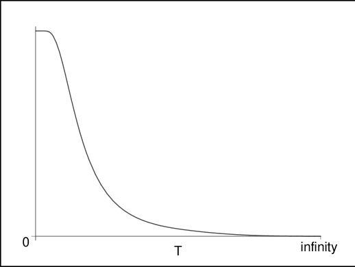
where the following notation $a={\displaystyle\frac{\beta\Lambda_{c}}{\pi}}\sqrt{1+(m/\Lambda_{c})^{2}}\approx{\displaystyle\frac{\beta\Lambda_{c}}{\pi}}$ was introduced. The curve depicted in Fig. 2 represents (in an arbitrary scale) the modulus $\sqrt{\theta_{\mu}^{2}}$ of the radiatively induced thermal Chern-Simons vector $\theta^{\mu}\,=\,(\theta^{0},0,0,0)$ with

$$\theta^{0}(T)\,=\,b^{0}\frac{e^{2}}{(2\pi)^{2}}\left[-\pi a+\pi a\tanh(\frac{\pi a}{2})^{2}+2\tanh(\frac{\pi a}{2})\right]$$

as a function of temperature, obtained from expression (13). It should be noticed, that the obtained coefficient has reasonable limiting values both at $T=0$ and at $T\to\infty$. The first one is $\Pi_{\mu\nu}^{A}(T=0)=i{\displaystyle\frac{e^{2}\varepsilon_{\mu\nu\alpha 0}k^{\alpha}b^{0}}{2\pi^{2}}}$, and it reproduces the result obtained earlier 14 for the case of vanishing temperature. At $T\rightarrow\infty$, we have $\Pi_{\mu\nu}^{A,T}\rightarrow 0$, which means, that at high temperatures, the Chern-Simons term generation is completely suppressed and, as a consequence, the Lorentz and CPT symmetries are completely restored.

Figure 2: Temperature dependence of the modulus $\sqrt{\theta(T)_{\mu}^{2}}$ of the induced CS vector .

III The Effective Potential.

In this section we shall consider the influence of a background non-abelian gauge field on the quark loop in the above model with an axial vector field. In order to calculate the effective potential of the model under these conditions, we shall use the method based on exact solutions of wave equations that can be obtained for certain simple configurations of background gauge fields. We adopt a model of quarks in the fundamental representation of the $SU(2)_{C}$ color group interacting with a non-abelian gauge field $A_{\mu}=A_{\mu}^{a}T_{a}$ and also with an electromagnetic field $F_{\mu\nu}$ and an axial-vector field $b_{\mu}$. Assuming slow variation of the color field on the hadronic scale, let us consider, as a first approximation, a constant non-abelian field $G_{\mu\nu}=$const. We consider the nonabelian background field to be rotationally-symmetric (a configuration, which is not possible in the abelian case)

$$A_{a}^{i}=\delta_{a}^{i}\sqrt{\lambda},\,\ \!\!\!\!\!\!\! A_{a}^{0}=0,\,\ G_{ik}^{a}=g\varepsilon_{ika}\lambda,$$ (14)

$$\lambda=\rm{const}>0.$$

We shall assume for later convenience that the following inequality is valid for the fields introduced

$$b_{0}^{2}\ll g^{2}\lambda\ll m^{2},$$ (15)

although, until special reference to this, we shall not use this condition. In these fields, the modified Dirac equation looks as follows:

$$(\gamma^{\mu}\Pi_{\mu}-b_{\mu}\gamma^{\mu}\gamma_{5}-m)\psi=0,$$ (16)

where $\Pi_{\mu}=p_{\mu}-gA_{\mu}^{a}T_{a}$. In order to find the spectrum of stationary states, it is convenient to consider the squared Dirac equation

$$\left(\Pi^{2}-2(\Pi b)\gamma_{5}-2\hat{b}\gamma_{5}\hat{\Pi}-m^{2}-b^{2}+\frac{1}{2}g\sigma^{\mu\nu}G_{\mu\nu}^{a}T_{a}\right)\psi=0,$$ (17)

or in matrix form

$$(\varepsilon^{2}-\hat{K})\psi=0,$$ (18)

where operator $\hat{K}$, according to (14), has the following structure

$$\hat{K}=\!\!\!\!\! \vec{p}^{2}+m^{2}+b_{0}^{2}+\frac{3}{4}g^{2}\lambda-\frac{1}{2}g^{2}\lambda(\vec{\Sigma}\vec{\tau})-g\sqrt{\lambda}(\vec{p}\vec{\tau})-$$ (19)

$$-2b_{0}\gamma_{0}\gamma_{5}(\vec{p}-\frac{1}{2}g\sqrt{\lambda}\vec{\tau})\vec{\gamma},$$

where $\vec{\Sigma}=\left(\begin{array}[]{cc}\vec{\sigma}&0\\ 0&\vec{\sigma}\end{array}\right)$, and $\vec{\sigma},\,\vec{\tau}$ are Pauli matrices belonging to spin and color spaces, respectively.

Hence, it is simple to obtain the following equation for the quark spectrum in the background color field

$$\bigg{(}{\vec{p}}^{2}(g^{2}\lambda+4b_{0}^{2})-a^{4}+{\displaystyle\frac{1}{4}}g^{2}\lambda x^{2}\bigg{)}^{2}-g^{2}\lambda\bigg{(}4{\vec{p}}^{2}b_{0}-$$

$$-a^{2}x+{\displaystyle\frac{1}{2}}g\sqrt{\lambda}x^{2}\bigg{)}^{2}=0,$$ (20)

where we have introduced the notations $a^{2}={\vec{p}}^{2}+m^{2}+b_{0}^{2}+\frac{3}{4}g^{2}\lambda-\varepsilon^{2}$ and $x=g\sqrt{\lambda}+b_{0}$.

Solving this equation, we receive four branches of the spectrum

$$\left\{\begin{array}[]{ll}\varepsilon_{1,2}^{2}=\bigg{(}|\vec{p}|\pm{\displaystyle\frac{1}{2}}(g\sqrt{\lambda}-2b_{0})\bigg{)}^{2}+m^{2}>0,\\ \cr\varepsilon_{3,4}^{2}=\bigg{(}\sqrt{{\vec{p}}^{2}+g^{2}\lambda}\pm{\displaystyle\frac{1}{2}}(g\sqrt{\lambda}+2b_{0})\bigg{)}^{2}+m^{2}>0.\\ \end{array}\right.$$

The squared fermion energies are required to be positive as the necessary condition for the theory to be free from having any tachyonic modes. With the above values for the spectrum it does not make any problem now to perform the standard kinematic considerations 14 , and obtain the value for the cut off constant from (III) using (15)

$$\Lambda_{c}=\frac{4m^{2}}{g\sqrt{\lambda}-2b_{0}}\approx\frac{4m^{2}}{g\sqrt{\lambda}}\gg m.$$ (21)

The one-loop effective action is defined as

$$W_{E}^{(1)}=\tau\int\frac{dq_{4}}{2\pi}\sum_{r}\ln{(q_{4}^{2}+\varepsilon_{r}^{2})},$$ (22)

where $\tau$ is the time interval in euclidian space-time, and summation over $r$ is assumed to run over all quantum numbers of quarks, including all spectrum branches, as well as over continuum of spatial components of the quark momentum. Using the formula

$$\ln{(A/B)}=-\int\limits_{0}^{\infty}\frac{ds}{s}(\exp{(-sA)}\,-\,\exp{(-sB)})$$

and performing integration over $q_{4}$, we get for the effective potential $V_{\hbox{eff}}^{(1)}=-{\displaystyle\frac{W_{E}^{(1)}}{\tau L^{3}}},$

$$V_{\hbox{eff}}^{(1)}=\frac{1}{L^{3}}\frac{1}{2\sqrt{\pi}}\sum\limits_{r}\int\limits_{0}^{\infty}\frac{ds}{s^{3/2}}\exp{(-s\varepsilon_{r}^{2})}\,-\,{\hbox{c.t.}},$$ (23)

where c.t. stands for the counter term such that $V_{\hbox{eff}}^{(1)}(b_{0}=g\sqrt{\lambda}=0)=0$. Taking into account that

$$\sum\limits_{r}=\frac{L^{3}}{(2\pi)^{3}}\int d^{3}p\sum\limits_{n}=\frac{4\pi L^{3}}{(2\pi)^{3}}\int\limits_{0}^{\infty}p^{2}dp\sum\limits_{n},$$

where summation $\sum\limits_{n}$ runs only over the spectrum branches, and introducing the following notations $z=sm^{2}$, $x={\displaystyle\frac{|\vec{p}|}{m}}$, $\phi^{2}={\displaystyle\frac{g^{2}\lambda}{m^{2}}}$ and $\psi^{2}={\displaystyle\frac{b_{0}^{2}}{m^{2}}}$, we rewrite the effective potential (23) in the form

$$\!\!\!V_{\rm eff}^{(1)}=\frac{m^{4}}{4\pi^{5/2}}\int\limits_{0}^{\infty}\frac{dz}{z^{3/2}}\int\limits_{0}^{\infty}dxx^{2}\sum\limits_{\nu=\pm 1}e^{-z\left(1+x^{2}\right)}\times$$ (24)

$$\!\!\!\!\!\!\!\!\!\!\!\!\times\bigg{[}e^{-z\left(1/4\phi^{2}-\phi\psi+\psi^{2}+\nu(\phi-2\psi)x\right)}+e^{-z\left(5/4\phi^{2}+\phi\psi+\psi^{2}+\nu(\phi+2\psi)\sqrt{x^{2}+\phi^{2}}\right)}-2\bigg{]}.$$ (25)

The last item in the brackets is the counter term. To calculate the integral (25), we make an expansion of the integrand in powers of small parameters $\phi,\psi\ll 1$. It is important to mention that, in the general case, the result depends on the order in which integrations are performed, i.e.,

$$\int\limits_{0}^{\infty}{\displaystyle\frac{dz}{z^{3/2}}}e^{-z}\int\limits_{0}^{\infty}dxx^{2}e^{-zx^{2}}f(z,x)$$

or

$$\int\limits_{0}^{\infty}dxx^{2}\int\limits_{0}^{\infty}{\displaystyle\frac{dz}{z^{3/2}}}e^{-z(1+x^{2})}f(z,x),$$

where $f(z,x)$ is the integrand after expansion. The reason for this is that both expressions, generally speaking, are divergent. This ambiguity can be eliminated when we apply a certain regularization procedure, for instance the physical cut off regularization. This means the integration over $x={\displaystyle\frac{|\vec{p}|}{m}}$ should be limited from above by the cut off (21)

$$M=\Lambda_{c}/m={\displaystyle\frac{4m}{g\sqrt{\lambda}}}.$$

Further calculations are made with the help of the relation

$$\int\limits_{0}^{\infty}\frac{dz}{z^{3/2}}e^{-z(1+x^{2})}z^{n}=(1+x^{2})^{(\frac{1}{2}-n)}\Gamma(n-\frac{1}{2}).$$

Thus, eventually, for the one-loop effective potential, we obtain

$$V_{\hbox{eff}}^{(1)}=\frac{m^{4}}{4\pi^{2}}\left(I_{\phi}+I_{\psi}+I_{\phi\psi}\right),$$ (26)

where

$$\!\!\!\!\!\!\!\!\!\!\!\!\!\!\!\!\!\!\!\!\!\!\!\!\!\!\!\!\!\!\!\!\!\!\!\!\!\!\!\!\!\!\!\!\!I_{\phi}=\!\!\!\!\!\! -\frac{M^{3}}{\sqrt{1+M^{2}}}\phi^{2}+\frac{1}{48}\Bigg{(}24\ln{(M+\sqrt{M^{2}+1})}-\frac{24M+35M^{3}+14M^{5}}{(1+M^{2})^{5/2}}\Bigg{)}\phi^{4}-$$ (27)

$$-\frac{1}{384}M^{3}\Bigg{(}\frac{183+408M^{2}+312M^{4}+80M^{6}}{(1+M^{2})^{9/2}}\Bigg{)}\phi^{6}+O\left(\phi^{8}\right),$$

$$\!\!\!\!\!\!\!\!\!\!\!\!I_{\psi}= \!\!\!\!\!\!\!4\left(\frac{M}{\sqrt{1+M^{2}}}-\ln{(M+\sqrt{M^{2}+1})}\right)\psi^{2}+\frac{1}{3}M^{3}\frac{1-2M^{2}}{(1+M^{2})^{5/2}}\psi^{4}+O\left(\psi^{6}\right),$$

$$\!\!\!\!\!\!\!\!\!\!\!\!\!\!\!\!\!\!\!\!\!\!\!\!\!\!\!\!\!\!\!\!\!\!\!\!\!\!\!\!\!\!\!\!\!\!\!\!\!\!\!\!\!\!\!\!I_{\psi\phi}=\frac{M^{3}}{(1+M^{2})^{3/2}}\psi\phi^{3}-\frac{3}{2}\frac{M^{3}}{(1+M^{2})^{5/2}}\psi^{2}\phi^{2}+O\left(\phi^{3}\psi^{3}\right).$$

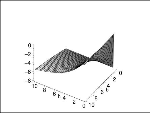
The plot of the effective potential $V_{\hbox{eff}}^{(1)}$ as a function of chromomagnetic and axial-vector fields is depicted in Fig. 3, where the effective potential is measured in units of ${\displaystyle\frac{m^{4}}{4\pi^{2}}}$, and dimensionless parameters $h$ and $b$ for the color field and axial-vector field are defined as $h={\displaystyle\frac{g\sqrt{\lambda}}{m}}\times 10^{-2}$ and $b={\displaystyle\frac{b_{0}}{m}}\times 10^{-3}$, respectively. The analysis of this plot demonstrates that with increasing strength of the color field the contribution of the axial-vector component decreases.

Figure 3: The effective potential $V_{\hbox{eff}}^{(1)}$ as a function of chromomagnetic and axial-vector field dimensionless parameters $h={\displaystyle\frac{g\sqrt{\lambda}}{m}}\times 10^{-2}$ and $b={\displaystyle\frac{b_{0}}{m}}\times 10^{-3}$.

Let us address to the part of (27), which corresponds to the pure chromomagnetic field contribution $I_{\phi}$. Despite the presence of terms of the order of $O(\phi^{2})$ and $O(\phi^{4})$ in the expression, the real contribution of the color field to the effective potential is provided only by the term of the order $O(\phi^{6})$. This happens because the formal limit of the first term $-M^{2}\phi^{2}$ at $M\rightarrow\infty$ is a pure number, and its contribution disappears, when one considers the limit of the whole expression (26) (this corresponds to the point $(h,b)=(0,0)$ in Fig. 3, where the effective potential vanishes, according to our choice of the counter term). As for the term $O(\phi^{4})$, its leading contribution with $M\to\infty$ has the form ${\displaystyle\frac{1}{8\pi^{2}}}\ln{(M)}m^{4}\phi^{4}\sim\ln{({\displaystyle\frac{m^{2}}{gH}})}(gH)^{2}$, where $H=\sqrt{3}g\lambda$ is the field strength, defining, thereby, the renormalized values of the field and the charge. Thus, the first nontrivial finite contribution looks as $I_{\phi^{6}}=-{\displaystyle\frac{5}{24}}\bigg{(}{\displaystyle\frac{gH}{m^{2}\sqrt{3}}}\bigg{)}^{3}$, which exactly coincides with the result obtained in 17 (actually, this is true for the term $O(\phi^{8})$ as well). This result differs from the case of the abelian fields, where the lowest term in the expansion of the one-loop effective potential is of the order of the fourth power of the field strength $O(gH)^{4}$, whereas, in the nonabelian theory, besides quadratic parameters like $F_{\mu\nu}^{2}$ and $F_{\mu\nu}\tilde{F^{\mu\nu}}$, new invariant parameters, such as the cubic one $F_{\mu\nu}^{a}F^{\nu b}_{\lambda}F^{\lambda\mu}_{c}\varepsilon_{abc}$ are possible, and they may form the lowest correction of the type obtained above.

IV Radiative correction to the CS coefficient in the presence of a weak color magnetic field

In this section, we shall demonstrate how the presence of a color magnetic field corrects the value of the induced Chern-Simons vector 14 . To this end, we calculate the antisymmetric part of the polarization operator, when both chromomagnetic and axial-vector fields are present in the background. The modified fermion propagator, in this case, takes the form

$$S(p)=\frac{i}{\hat{\Pi}-m-\hat{b}\gamma_{5}},$$ (28)

where, as before, $\Pi_{\mu}=p_{\mu}-gA_{\mu}^{a}T_{a}$. This expression may be rewritten as

$$S(p)=i{\displaystyle\frac{\hat{\Pi}+m+\hat{b}\gamma_{5}}{\Pi^{2}+2(\Pi b)\gamma_{5}-2m\hat{b}\gamma_{5}-m^{2}+b^{2}+\frac{1}{2}g(\sigma G)}}.$$ (29)

Taking the following relation into consideration $\left[\gamma_{5},\sigma_{ik}\right]=\left[\gamma_{0}\gamma_{5},\sigma_{ik}\right]=0$ for $i,k=\overline{1,3}$, one can perform, for the background field configuration (14) admitted, a correct expansion of the propagator in powers of $b$ restricting oneself, as before, to the term linear in $b_{0}$. This results in

$$S(p)=i\left(\hat{\Pi}+m+\hat{b}\gamma_{5}\right)\left[{\displaystyle\frac{1}{\Pi^{2}-m^{2}+1/2g(\sigma G)}}-{\displaystyle\frac{2(\Pi b)\gamma_{5}-2m\hat{b}\gamma_{5}}{\left(\Pi^{2}-m^{2}+1/2g(\sigma G)\right)^{2}}}\right].$$ (30)

Further, taking into account, that the antisymmetric part of PO appears as a structure proportional to an antisymmetric tensor, we expand (30) in powers of $(\sigma G)$ and keep only the linear term. Then,

$$S(p)\!\!\!\!\!\!\! =i\bigg{[}A+B\gamma_{5}+C_{\mu}\gamma^{\mu}+D_{\mu ik}\gamma^{\mu}\sigma^{ik}+E_{ik}\sigma^{ik}+F_{ik}\gamma_{0}\gamma_{5}\sigma^{ik}+I\gamma_{0}\gamma_{5}+J_{\mu}\gamma_{\mu}\gamma_{5}+K_{\mu}\gamma^{\mu}\gamma_{0}\gamma_{5}+$$ (31)

$$+L_{\mu ik}\gamma^{\mu}\sigma^{ik}\gamma_{5}+M_{\mu ik}\gamma^{\mu}\sigma^{ik}\gamma_{0}\gamma_{5}+N_{ik}\sigma^{ik}\gamma_{5}\bigg{]},$$

where we have introduced a new notations for

$$\!\!\!\!\!\!\!\!A={\displaystyle\frac{m}{\Delta}},\,\,B=-\frac{2mb_{0}p_{0}}{\Delta^{2}},\,\,C_{\mu}=\frac{\Pi_{\mu}}{\Delta},\,\,D_{\mu ik}=-\frac{\Pi_{\mu}gG_{ik}}{2\Delta^{2}},\,\,E_{ik}=-\frac{mgG_{ik}}{2\Delta^{2}},\,\,F_{ik}=-\frac{b_{0}gG_{ik}}{2\Delta^{2}}\bigg{(}1+\frac{2m^{2}}{\Delta}\bigg{)},$$

$$\!\!\!\!\!\!\!\!I=\frac{b_{0}}{\Delta}\bigg{(}1+\frac{2m^{2}}{\Delta}\bigg{)},\,\,J_{\mu}=-\frac{2p_{0}b_{0}\Pi_{\mu}}{\Delta^{2}},\,\,K_{\mu}=\frac{2mb_{0}\Pi_{\mu}}{\Delta^{2}},\,\,L_{\mu ik}=\frac{2p_{0}b_{0}\Pi_{\mu}gG_{ik}}{\Delta^{3}},\,\,M_{\mu ik}=-\frac{2m\Pi_{\mu}gG_{ik}b_{0}}{\Delta^{3}},$$

$$\!\!\!\!\!\!\!\!N_{ik}=\frac{2mp_{0}b_{0}gG_{ik}}{\Delta^{3}}$$ (32)

with $\Delta=\Pi^{2}-m^{2}$.

The polarization operator is defined as before (see (1)), where the trace operation now should be perform over color indices as well. In order to obtain the antisymmetric part of PO, we have to calculate the trace over spinor indices. Excluding from the resulting expression the terms that refer to the pure color magnetic field, we obtain

$$\Pi^{A}_{\rho\sigma}\!\!\!\!\!\! =-ie^{2}{\rm tr}_{c}\int\frac{d^{4}p}{(2\pi)^{4}}\Bigg{[}4i\varepsilon_{\rho\sigma\mu 0}(K_{1}^{\mu}A_{2}-K_{2}^{\mu}A_{1})+4(g_{\rho\delta}g_{\sigma\mu}-g_{\rho\mu}g_{\sigma\delta})\varepsilon_{ik0\delta}(M_{1}^{\mu ik}A_{2}-A_{1}M_{2}^{\mu ik})+$$ (37)

$$+4\varepsilon_{\rho\sigma ik}(A_{1}N_{2}^{ik}-N_{1}^{ik}A_{2})+4i\varepsilon_{\rho\sigma\mu 0}(C_{1}^{\mu}I_{2}-I_{1}C_{2}^{\mu})+4i\varepsilon_{\rho\sigma\mu\nu}(C_{1}^{\mu}J_{2}^{\nu}-C_{2}^{\mu}J_{1}^{\nu})+4\varepsilon_{\rho\sigma\mu\delta}(g_{i\nu}g_{k\delta}-$$

$$-g_{k\nu}g_{i\delta})(C_{1}^{\mu}L_{2}^{\nu ik}-L_{1}^{\nu ik}C_{2}^{\mu})-4i\varepsilon_{ik\mu\delta}\varepsilon_{lm0\alpha}\varepsilon_{\rho\sigma\alpha\delta}(D_{1}^{\mu ik}F_{2}^{lm}-F_{1}^{lm}D_{2}^{\mu ik})+4\varepsilon_{\rho\sigma\delta 0}(g_{i\mu}g_{k\delta}-g_{k\mu}g_{i\delta})\times$$

$$\times(D_{1}^{\mu ik}I_{2}-I_{1}D_{2}^{\mu ik})+4\varepsilon_{\rho\sigma\delta\nu}(g_{i\mu}g_{k\delta}-g_{k\mu}g_{i\delta})(D_{1}^{\mu ik}J_{2}^{\nu}-J_{1}^{\nu}D_{2}^{\mu ik})+4i\varepsilon_{\rho\sigma\alpha\delta}\bigg{(}(g_{i\mu}g_{k\delta}-g_{k\mu}g_{i\delta})\times$$

$$\times(g_{l\nu}g_{m\alpha}-g_{m\nu}g_{l\alpha})-\varepsilon_{ik\mu\delta}\varepsilon_{lm\nu\alpha}\bigg{)}(D_{1}^{\mu ik}L_{2}^{\nu lm}-L_{1}^{\nu lm}D_{2}^{\mu ik})+E_{1}^{ik}K_{2}^{\mu}\bigg{(}4\varepsilon_{ik\rho\delta}(g_{\delta\sigma}g_{\mu 0}-g_{\delta\mu}g_{\sigma 0}+g_{\delta 0}g_{\sigma\mu})-$$

$$-4\varepsilon_{\delta\sigma\mu 0}(g_{i\rho}g_{k\delta}-g_{k\rho}g_{i\delta})\bigg{)}+E_{2}^{ik}K_{1}^{\mu}\bigg{(}\rho\leftrightarrow\sigma\bigg{)}+E_{1}^{ik}M_{2}^{\nu lm}\bigg{(}4i\varepsilon_{ik\rho\delta}\varepsilon_{lm0\alpha}\varepsilon_{\delta\alpha\sigma\nu}+4i\varepsilon_{lm0\alpha}\times$$

$$\times(g_{i\rho}g_{k\delta}-g_{k\rho}g_{i\delta})(g_{\delta\sigma}g_{\nu\alpha}-g_{\delta\nu}g_{\sigma\alpha}+g_{\delta\alpha}g_{\sigma\nu})\bigg{)}+E_{2}^{ik}M_{1}^{\nu lm}\bigg{(}\rho\leftrightarrow\sigma\bigg{)}\Bigg{]},$$

where indices 1 and 2 mean that we use (31) for $A,...,N^{ik}$, with $p$ replaced by $p\pm k/2$ respectively, symbol $(\rho\leftrightarrow\sigma)$ is used to denote the same expression as the previous one up to permutation of $\rho$ and $\sigma$, and ${\rm tr}_{c}$ stands for the trace over color indices.

Each integral in (37) has the general structure, which may be represented in the form

$$\int\frac{d^{4}p}{(2\pi)^{4}}\frac{\Phi_{\rho\sigma}(p,gA^{a}T_{a},m)}{(\Delta_{1}\Delta_{2})^{n}}.$$

Here, $\Delta_{1,2}=\Pi_{1,2}^{2}-m^{2}$, and $n=2,3$ for different integrals. It should be mentioned that in the static limit (the rest frame of reference) $(\vec{k}\rightarrow 0,\,k_{0}=0)$, the denominator is equal to $(\Delta_{1}\Delta_{2})^{n}=(p_{0}^{2}-(\vec{p}-g\vec{A}_{a}{\displaystyle\frac{\tau^{a}}{2}})^{2}-m^{2})^{2n}.$ Thus, expanding the integrand up to terms of the order $O(gA\tau)^{4}$ and calculating the trace over color indices, we integrate over $p$ with the upper limit equal to the constant $\Lambda_{c}$, as it was prescribed in the previous section. As a result, we obtain for the antisymmetric part of PO

$$\Pi_{\rho\sigma}^{A}=-ie^{2}\frac{2}{\pi^{2}}\varepsilon_{\rho\sigma\mu 0}k_{\mu}b_{0}\Bigg{[}-\frac{1}{2}+\frac{15}{32}\bigg{(}\frac{g\sqrt{\lambda}}{m}\bigg{)}^{2}+O\bigg{(}\frac{g\sqrt{\lambda}}{m}\bigg{)}^{4}\Bigg{]}.$$ (38)

We remind that the contribution of a pure color magnetic field to the antisymmetric part of PO is given by the formula 16

$$\Pi_{\rho\sigma}^{A}(b_{0}=0,\lambda\neq 0)=ie^{2}\frac{5}{24\pi^{2}}\varepsilon_{\rho\sigma\mu}k^{\mu}\frac{g^{3}\lambda^{3/2}}{m^{2}}.$$ (39)

The first term in the brackets of our result (38) refers to the induced Chern-Simons term $\Pi^{A}(b_{0}\neq~{}0,\lambda=0)$, when only the axial-vector field is present in the theory, and this is in complete agreement with the result, obtained in 14 . The second term gives the correction, calculated with both fields present $\triangle\Pi^{A}(b_{0}\neq 0,\lambda\neq 0)$, and its value depends on their relative strength

$$\frac{\triangle\Pi^{A}(b_{0}\neq 0,\lambda\neq 0)}{\Pi^{A}(b_{0}=0,\lambda\neq 0)}\sim\frac{b_{0}}{g\sqrt{\lambda}}\ll 1.$$

At the same time, the ratio of the contributions induced by the axial vector and the color fields separately

$$\frac{\Pi^{A}(b_{0}\neq 0,\lambda=0)}{\Pi^{A}(b_{0}=0,\lambda\neq 0)}\sim\frac{b_{0}}{g\sqrt{\lambda}}\bigg{(}\frac{m}{g\sqrt{\lambda}}\bigg{)}^{2}$$

substantially depends not only on the relation of the fields, but also on the ratio of the fermionic mass and the strength of the color field. Therefore, under the condition (15), when this ratio is large, the color field and the axial vector field may provide comparable contributions to the induced CS vector.

Conclusions

We have calculated the one-loop fermion contribution to the antisymmetric part of the photon polarization operator in an external constant axial-vector field $b_{\mu}$. The result was obtained in the linear order in the pseudo vector field, using the physical cut off regularization scheme. The analysis of the temperature dependence of the obtained expression allows us to conclude that generation of a Lorentz- and CPT-odd term may occur at any physical value of temperature. In particular, we have reproduced the standard result for the case of vanishing temperature, $T=0$, 14 . Moreover, we have shown that this effect is completely suppressed in the limit of very high temperature, $T\to\infty$, when the theory restores its Lorentz and CPT symmetries.

The influence of the vacuum field, modelled by a constant nonabelian color magnetic field, on generation of a Chern-Simons term has been considered in the one-loop approximation. We have constructed the effective potential for this model with consideration of both the axial-vector field and a nonabelian color field. We have demonstrated that with increasing strength of the color field the contribution of the axial-vector component to the effective potential decreases. The first nontrivial correction to the induced topological CS vector due to the presence of a weak (with respect to fermion mass) color magnetic field has been obtained and its relative contribution to the total CS coefficient has been estimated.

It is important to notice that the possible presence of an antisymmetric part of the photon polarization operator demonstrates spatial anisotropy. This may provide one of the physical mechanisms for possible unusual phenomena in the propagation of light through the universe, i.e., rotation of the plane of polarization of electromagnetic radiation propagating over cosmological distances (the effect, different from the usual Faraday rotation, which was discussed in recent publications 2 ).

In the present work, as in the series of papers mentioned in the Introduction, we have used the extended model of QED, where the Lorentz and CPT non-covariant interaction term for fermions (a constant axial-vector field) is present. Interactions of photons with fermion loops in this background field lead to the phenomena mentioned above. However, it should be mentioned that the dynamical origin of this pseudovector field, in spite of numerous efforts, still remains to be explained 5 ; 6 ; 7 .