Classical Stability of Black D3-branes

Abstract

We have investigated the classical stability of charged black $D3$-branes in type IIB supergravity under small perturbations. For $s$-wave perturbations it turns out that black $D3$-branes are unstable when they have small charge density. As the charge density increases for given mass density, however, the instability decreases down to zero at a certain finite value of the charge density, and then black $D3$-branes become stable all the way down to the extremal point. It has also been shown that such critical value at which its stability behavior changes agrees very well with the predicted one by the thermodynamic stability behavior of the corresponding black hole system through the Gubser-Mitra conjecture. Unstable mode solutions we found involve non-vanishing fluctuations of the self-dual five-form field strength. Some implications of our results are also discussed.

I Introduction

It is well known that the four-dimensional Schwarzschild black hole in Einstein gravity is stable classically under linearized perturbations. Recently, Ishibashi and Kodama Ishibashi:2003ap have shown that this stable behavior extends to hold for higher dimensional cases. However, some black strings or branes, which have hypercylindrical horizons instead of compact hyperspherical ones, are found to be unstable as the compactification scale of extended directions becomes larger than the order of the horizon radius - the so-called Gregory-Laflamme instability GL1 . The simplest black string would be the five-dimensional Schwarzschild black string in Einstein gravity that is a foliation of four-dimensional Schwarzschild black holes along the fifth direction.

Gregory and Laflamme Gregory:1994bj also considered a class of magnetically charged black $p$-brane solutions for a stringy action containing the NS5-brane of the type II supergravity. For horizons with infinite extent, they have shown that the instability persists to appear but decreases as the charge increases to the extremal value. On the other hand, branes with extremal charge turned out to be stable Gregory:1994tw . Since their discovery of such linearized instability, black strings or branes have been believed to be generically unstable classically under small perturbations except for the cases of extremal or suitably compactified ones, and the Gregory-Laflamme instability has been used to understand physical behaviors of various systems involving black brane configurations as in string theory. Recently, however, Hirayama and Kang Hirayama:2001bi analyzed the stability of three types of black string backgrounds in five-dimensional AdS space. With or without the presence of a 3-brane, the geometry of these black strings in consideration is warped in the fifth direction, resulting in no translational symmetry along the horizon. They showed that the AdS₄-Schwarzschild black string becomes stable as the horizon radius is larger than the order of the AdS₄ radius whereas Schwarzschild Gregory:2000gf and dS₄-Schwarzschild black strings are unstable as usual. It is possible to have stationary black string or brane solutions even in four dimensions when a negative cosmological constant is present. Interestingly it seems that all known stationary black branes in four dimensions are stable. In particular, the case of BTZ black strings has been checked explicitly Kang:2002hx .

In the context of string theory black branes that Gregory and Laflamme considered are those having magnetic charges with respect to Neveu-Schwarz gauge fields only Gregory:1994bj . Having found some black string systems in which the Gregory-Laflamme instability is absent as mentioned above, Hirayama, Kang, and Lee Hirayama:2002hn have also considered a wider class of black brane solutions for string gravity in order to see whether or not the stability behavior drastically changes. Indeed it turns out that the stability of black branes behaves very differently depending on the parameter $a$ that specifies the strength of coupling between dilaton and gauge fields in the theory as in Eq. (1) below. That is, for magnetically charged static black brane solutions in theories of this form Duff:1996hp , there exists a critical value of the coupling parameter $a_{\rm cr}(D,p)$ to be determined by the full spacetime dimension $D$ and the dimension of the spatial worldvolume $p$ of those black $p$-branes. The case that Gregory and Laflamme studied is precisely when $a=a_{\rm cr}$. Black branes with horizons of infinite extent in this case are always unstable as explained above, and magnetically charged NS5-branes of the type II supergravity belong to this class. When $0<a<a_{\rm cr}$, black branes with small charge are unstable as usual. As the charge increases, however, the instability decreases and eventually disappears at a certain critical value of the charge density which could be even far from the extremal point. Magnetically charged black D0, F1, D1, D2, D4 branes of the type II string theory belong to this class for instance. When $a>a_{\rm cr}$, on the other hand, the instability persists all the way down to the extremal point. Magnetically charged black D5 and D6 branes are in this case for example. However it is shown that all black branes mentioned above are stable at the extremal point, which might be expected due to the BPS nature of extremal solutions in string theory.

Recently, Gubser and Mitra Gubser:2000ec gave a conjecture about when the classical instability of a black brane sets on in terms of thermodynamic stability. This Gubser-Mitra (GM) conjecture is a sort of refinement of the entropy comparison argument given by Gregory and Laflamme GL1 ; Gregory:1994bj , and states that a black brane with a non-compact translational symmetry is classically stable if and only if it is locally thermodynamically stable. As argued by Reall Reall:2001ag , when we expand classical perturbations in terms of Fourier modes along the horizon having translational symmetry, the set of linearized perturbation equations for a black brane becomes the Lichnerowitz equation with an additional mass term for the black hole on horizon cross sections. Now it can be seen that the existence of a threshold mode for instability of a black brane is related to the presence of a negative eigen mode in the Euclidean path integral for the black hole system. Consequently, the partition function gets an imaginary contribution, implying a thermodynamic instability of the black hole system on the horizon cross sections, and vice versa. This interesting relationship between classical dynamical and local thermodynamic stabilities has been checked explicitly for various black string or brane systems Gubser:2000ec ; Kang:2002hx ; Hirayama:2002hn ; PGR ; Gubser:2002yi . When the translational symmetry along the horizon is broken, one can see some disagreements for on set points for instability as shown in the stability analysis for AdS₄-Schwarzschild black strings in AdS space Hirayama:2001bi . It also should be pointed out that this conjecture simply gives the information about when a black string or brane becomes stable or unstable. It does not explain or predict other details of classical stability behaviors Hirayama:2002hn .

In the present paper, we analyze the classical stability of charged static black brane solutions for the theory in Eq. (1) in the case that $n=D/2$ (i.e., $a=0$) with a self-dual $n$-form field strength. This case includes black D3-branes in the type II supergravity, and is of interest for several reasons. Firstly, note that the geometry of the spatial worldvolume of black brane backgrounds whose linearized stabilities have been analyzed so far in the literature is flat. As can be seen in Eq. (4) below, however, black brane backgrounds to be considered in this paper do not have flat spatial worldvolume, but have a warping factor multiplied. Such overall factor can not be removed by finding a suitable conformally equivalent theory as in Refs. Reall:2001ag ; Hirayama:2002hn since the background dilaton field is constant in this case. Therefore a sort of Kaluza-Klein reduction of perturbation equations for these black branes does not give the standard form of the Lichnerowitz equation with an additional mass term for black holes on the horizon cross sections as usual. Secondly, in the $s$-wave perturbation analyses in Refs. Reall:2001ag ; Hirayama:2002hn , fluctuations of the field strength for unstable modes could be set to be zero consistently partly because black branes are charged magnetically only. However, black brane backgrounds in the consideration are charged electrically as well as magnetically since the five-form field strength is self-dual. Subsequently, it is not consistent to set $s$-wave fluctuations of the field strength being frozen as shall be shown below explicitly. Finally, the case of black $D3$-brane is not included in the proof of the GM conjecture by Reall Reall:2001ag . Although he suggests some generalization of the argument in Ref. Reall:2001ag could include the case, such generalization seems to be non-trivial for the reasons mentioned above. Moreover, the covariant action including a self-dual field strength is not known, and so it is not clear how the self-duality condition could be incorporated in the proof. Therefore it is interesting to see not only how different features mentioned above affect the detailed stability analysis for black branes to be considered in this paper, but also whether or not the GM conjecture still holds for these “dyonic” branes.

Actually the classical stability of the black D3-brane has been studied by using a notion of universality classes recently by Gubser and Ozakin Gubser:2002yi . For s-wave fluctuations they dimensionally reduce the ten-dimensional type IIB supergravity action to a three-dimensional one that contains gravity and two scalar fields only, and perform there the stability analysis for static perturbations in a certain specific form. However it is not clear whether or not all relevant perturbations in the original theory have been covered in such analysis. In particular, the field strength is assumed to be frozen in their dimensional reduction. Although such approximation would be of little significance for small charge, it might change the stability behavior significantly as the charge increases. Finally, we would like to point out that in string theory the system of D3-branes is understood best in the context of the AdS/CFT correspondence. Hence the details of stability behavior in gravity side might be very useful for understanding corresponding behaviors in the CFT side.

In section II, we briefly summarize the local thermodynamic behaviors of black D3-branes in order to get a hint at the classical stability predicted by the Gubser-Mitra conjecture. In section III, we perform the perturbation analysis explicitly and give numerical results. Finally, some possible physical implications of our results are discussed.

II Thermodynamic behavior

Let us consider the action given by

$${\rm I} = \int d^{D}x\sqrt{-\bar{g}}\left[e^{-2\bar{\phi}}\left(\bar{R}+4(\partial\bar{\phi})^{2}\right)-\frac{1}{2n!}F_{n}^{2}\right]$$ (1)

$$= \int d^{D}x\sqrt{-g}\left[R-\frac{1}{2}(\partial\phi)^{2}-\frac{1}{2n!}e^{a\phi}F_{n}^{2}\right].$$

The second form is written in Einstein frame with $a=(D-2n)/\sqrt{2(D-2)}$. It is known that there is no covariant action for low energy type IIB supergravity due to the self-duality condition for the field strength ${\bf F}_{5}=\mbox{}^{*}{\bf F}_{5}$. However, the action in Eq. (1) with $D=10$ and $n=5$ is quite close to the type IIB supergravity with all other form fields set to be zero. When the rank of the field strength is $n=D/2$, one has $a=0$ and the field equations for the action in Eq. (1) are given by

$$\nabla_{M}F^{MP_{1}\cdots P_{n-1}}=0,\qquad\qquad\nabla^{2}\phi=0,$$

$$R_{MN}=\frac{1}{2}\nabla_{M}\phi\nabla_{N}\phi+\frac{1}{2(n-1)!}F_{MP_{1}\cdots P_{n-1}}F_{N}^{P_{1}\cdots P_{n-1}}-\frac{1}{4n!}F^{2}g_{MN}.$$ (2)

In the following we consider a gravity theory in which the dynamics of fields is governed by the field equations given in Eq. (2) with an additional constraint of self-duality for the field strength on solutions such as

$${\bf F}=\mbox{}^{*}{\bf F}.$$ (3)

Static black $p$-brane solutions for this theory are Duff:1996hp

$$ds^{2}=-Udt^{2}+\frac{dr^{2}}{U}+R^{2}d\Omega_{n}^{2}+W\delta_{ij}dz^{i}dz^{j}$$

$$\qquad=W\left(-Ndt^{2}+\delta_{ij}dz^{i}dz^{j}\right)+W^{-1}\left(N^{-1}dr^{2}+r^{2}d\Omega_{n}^{2}\right),$$

$$\phi=0,\qquad\qquad{\bf F}=\lambda\left(\mbox{\boldmath$\epsilon$}_{n}+\mbox{}^{*}\mbox{\boldmath$\epsilon$}_{n}\right),$$ (4)

where

$$N=1-\frac{k}{r^{n-1}},\quad W=\left(1+\frac{k}{r^{n-1}}\sinh^{2}\mu\right)^{-2/(n-1)},\quad U=WN,\quad R^{2}=r^{2}W^{-1}.$$ (5)

Here $n=D/2=p+2$, the $p$-dimensional spatial worldvolume directions are denoted by $z^{i}$ with $i=1,2,\cdots,p$, and $\mbox{\boldmath$\epsilon$}_{n}$ is the volume form on the unit sphere $d\Omega_{n}^{2}$. The mass and both electric and magnetic charge densities are

$$M=k\left(n+4\sinh^{2}\mu\right),\qquad\lambda=\sqrt{\frac{n-1}{2}}k\sinh 2\mu,$$ (6)

respectively. Notice that the spatial worldvolume of this brane is not flat except for the uncharged case (i.e., $W=1$). The maximally charged extremal limit is $k\rightarrow 0$ and $\mu\rightarrow\infty$ with the mass density (or, $ke^{2\mu}$) fixed.

Now let us consider a finite segment of this black $p$-brane with unit worldvolume. Being regarded as a thermal system, it has entropy and temperature given by

$$S\sim\left(\cosh\mu\right)^{\frac{4}{n-1}}r_{\scriptscriptstyle{H}}^{n}\quad{\rm and}\quad T=\frac{n-1}{4\pi r_{\scriptscriptstyle{H}}}\left(\cosh\mu\right)^{-\frac{4}{n-1}},$$ (7)

respectively. Here $r_{\scriptscriptstyle{H}}=k^{1/(n-1)}$ is the horizon radius. The specific heat capacity is given by

$$C_{\lambda}=\left(\frac{\partial M}{\partial T}\right)_{\lambda}=-4\pi r_{\scriptscriptstyle{H}}^{n}\left(\cosh\mu\right)^{\frac{4}{n-1}}\,\,\frac{2+(n-2)\cosh 2\mu}{1-2\sinh^{2}\mu}.$$ (8)

Here one finds that, as $\mu$ increases, the heat capacity changes its sign from negativeness to positiveness at a certain critical value of $\mu$ given by

$$\sinh^{2}\mu_{\rm cr}=1/2.$$ (9)

Thus, if the Gubser-Mitra conjecture holds for this system as well, we expect that these black $p$-brane backgrounds become stable classically under small perturbations for $\mu\geq\mu_{\rm cr}$. Defining an extremality parameter as

$$q=\frac{\lambda}{\lambda_{\rm max}}=\frac{2\sinh 2\mu}{n+4\sinh^{2}\mu}$$ (10)

with $\lambda_{\rm max}=\sqrt{(n-1)/8}\,M$, one notice that this critical value corresponds to

$$q_{\rm cr}=\frac{2\sqrt{3}}{n+2}.$$ (11)

For the black D3-brane (i.e., $n=5$) this value is $q_{\rm cr}=2\sqrt{3}/7\simeq 0.495$.

III Perturbation analysis

In this section we perform the classical stability analysis for small perturbations of fields at the linear level. Under $\phi\rightarrow\phi+\delta\phi$, ${\mathbf{F}}\rightarrow{\mathbf{F}}+\delta{\mathbf{F}}$, and $g_{MN}\rightarrow g_{MN}+h_{MN}$, we have from Eq. (2) linearized perturbation equations given by

$$\nabla^{2}\delta\phi-\nabla_{(M}\nabla_{N)}\phi h^{MN}-\nabla_{(M}\phi\nabla_{N)}\Big{(}h^{MN}-\frac{1}{2}g^{MN}h\Big{)}=0,$$ (12)

$$\nabla_{M}\delta F^{MP_{1}\cdots P_{n-1}}-\nabla_{M}F^{QP_{1}\cdots P_{n-1}}h^{M}_{Q}$$

$$-(n-1)F^{MQ[P_{2}\cdot P_{n-1}}\nabla_{M}h^{P_{1}]}_{Q}-\nabla_{M}\Big{(}h^{M}_{Q}-\frac{1}{2}h\delta^{M}_{Q}\Big{)}F^{QP_{1}\cdot P_{n-1}}=0,$$ (13)

$$\nabla^{2}h^{M}_{N}+\nabla^{M}\nabla_{N}h-\nabla_{Q}\nabla^{M}h^{Q}_{N}-\nabla^{Q}\nabla_{N}h^{M}_{Q}+2\nabla^{(M}\phi\nabla_{N)}\delta\phi$$

$$+\frac{1}{(n-1)!}\bigg{(}2\delta F^{(M|P_{1}\cdots P_{n-1}|}F_{N)P_{1}\cdots P_{n-1}}-(n-1)F^{M}_{PR_{1}\cdot R_{n-2}}F^{QR_{1}\cdots R_{n-2}}h^{P}_{Q}\bigg{)}$$

$$-\frac{1}{2n!}\bigg{[}F^{2}h^{M}_{N}+\delta^{M}_{N}\Big{(}2F^{p_{1}\cdots P_{n}}\delta F_{P_{1}\cdots P_{n}}-nF_{PR_{1}\cdots R_{n-1}}F^{QR_{1}\cdots R_{n-1}}h^{P}_{Q}\Big{)}\bigg{]}=0$$ (14)

with the perturbed self-duality condition

$$\delta({\mathbf{F}}-\mbox{}^{*}\!{\mathbf{F}})=0.$$ (15)

It is very important to notice that the self-duality condition imposed on the perturbed field strength in Eq. (15) is not $\delta{\mathbf{F}}=\mbox{}^{*}\!\delta{\mathbf{F}}$, but

$$\delta F_{M_{1}\cdots M_{n}}=(\mbox{}^{*}\!\delta F)_{M_{1}\cdots M_{n}}+\frac{1}{2}hF_{M_{1}\cdots M_{n}}-\frac{1}{(n-1)!}h^{PQ}F^{P_{1}\cdots P_{n-1}}_{Q}\epsilon_{PP_{1}\cdots P_{n-1}M_{1}\cdots M_{n}}.$$ (16)

In addition the Bianchi identity requires

$$d\,\delta{\mathbf{F}}=0.$$ (17)

In order to see whether or not the black $p$-brane backgrounds in Eq. (4) are stable under small perturbations, we need to check if there is any solution for linearized equations given above that is growing in time while it is regular spatially outside the event horizon. In case that the black brane is stable, it would be very difficult to show there exists no such unstable solution in general. When the black $p$-brane background is unstable, however, it is rather easy to find a certain type of unstable solutions. Notice first that, since the background dilaton field is constant, the fluctuation of the dilaton field can be seen from Eq. (12) to be completely decoupled, i.e., $\nabla^{2}\delta\phi=0$. Hence one can set $\delta\phi=0$. Since the background fields in Eq. (4) are stationary and invariant under translations in directions of the spatial worldvolume, one can also assume that

$$\delta{\mathbf{F}}(x^{\mu},z^{i})=e^{\Omega t+im_{i}z^{i}}\delta{\mathbf{F}}(r,\theta^{m}),\qquad h_{MN}(x^{\mu},z^{i})=e^{\Omega t+im_{i}z^{i}}H_{MN}(r,\theta^{m})$$ (18)

for unstable mode solutions. Here $\Omega>0$ and $\{\theta^{m}\}$ are angular coordinates for the $n$-sphere. We denote the coordinate system by $\{x^{M}\}=\{x^{\mu},z^{i}\}=\{t,r,\theta^{m},z^{i}\}$.

For $s$-wave perturbations that are spherically symmetric in submanifolds perpendicular to the $p$-dimensional spatial worldvolume, one can easily see that the Bianchi identity in Eq. (17) restricts the form of $\delta{\mathbf{F}}$ further, yielding the only non-vanishing components given by

$$\delta F_{trz^{1}\cdots z^{p}}=e^{\Omega t+im_{i}z^{i}}Q(r).$$ (19)

In order to see the presence of unstable mode solutions, it suffices to consider the threshold modes (i.e., $\Omega=0$) only as usual PGR ; Hirayama:2002hn ; Reall:2001ag . Note that we have not imposed any gauge such as the transverse gauge (e.g., $\nabla_{M}h^{MN}=\nabla^{N}h/2$) for metric perturbations $h_{MN}$ in Eq. (14) so far. For unstable threshold modes one may set $H_{tr}=H_{ti}=0$ by choosing a suitable gauge as in Refs. PGR ; Reall:2001ag , instead of the usual transverse gauge as in Gregory and Laflamme Gregory:1994bj . Now the remaining non-vanishing components of $H_{MN}$ are $H_{tt}$, $H_{rr}$, $H_{ri}$, $H_{\theta\theta}$ and $H_{ij}$. By looking at the form of perturbation equations for $H_{ij}$ and $H_{ri}$, one may have

$$H^{i}_{j}=\frac{m_{i}m_{j}}{m^{2}}\zeta(r)+\delta^{i}_{j}\rho(r)$$ (20)

and

$$H^{r}_{i}=i\frac{m_{i}}{m}\eta(r),$$ (21)

where $m^{2}=\sum^{p}_{i=1}m^{2}_{i}$. If $\rho=0$, this is exactly the same ansatz used by Gregory and Laflamme Gregory:1994bj . The presence of the new term $\rho$ above can be understood as follows. Under the diffeomorphisms associated with a vector field $\xi^{M}=e^{im_{i}z^{i}}\xi^{M}(r)$, we have

$$\tilde{H}_{ij}=H_{ij}-im_{i}\xi_{j}(r)-im_{j}\xi_{i}(r)-\delta_{ij}V\left(\frac{W^{\prime}}{W}\right)\xi_{r}(r).$$ (22)

Since $W^{\prime}=\partial_{r}W$ does not vanish for charged black branes, the term $\rho$ should appear in general. On the other hand, the $H_{ri}$ component transforms as

$$\tilde{H}_{ri}=H_{ri}-im_{i}\xi_{r}(r)-\xi^{\prime}_{i}(r)+\frac{W^{\prime}}{W}\xi_{i}(r).$$ (23)

Therefore, when the spatial worldvolume of a black brane is a warped flat space as in the present case, one sees that only two of three functions $\zeta$, $\rho$ and $\eta$ can be eliminated by choosing suitable functions $\xi_{r}(r)$ and $\xi(r)$ in $\xi_{i}(r)=im_{i}\xi(r)$. We set $\zeta=\eta=0$ in our analysis. Consequently, for threshold modes the non-vanishing components of $s$-wave metric perturbations finally become

$$h^{M}_{N} = e^{im_{i}z^{i}}{\rm diag}\left(H^{t}_{t},H^{r}_{r},H^{\theta^{m}}_{\theta^{m}},H^{i}_{i}\right)$$ (24)

$$= e^{im_{i}z^{i}}{\rm diag}\left(\varphi,\psi,\chi,\cdots,\chi,\rho,\cdots,\rho\right),$$

where all unknown functions $\varphi,\psi,\chi,$ and $\rho$ are functions of the radial coordinate $r$ only.

In Appendix A, all linearized perturbation equations in Eqs. (13) and (14) are shown in components. We have seven coupled ordinary differential equations for seven unknown functions $\varphi$, $\psi$, $\chi$, $\zeta$, $\eta$, $\rho$ and $Q$. Although we have not used the transverse gauge condition, note that in the Reall gauge (i.e., $\zeta=\eta=0$) the linearized perturbation equation Eq. (67) becomes equivalent to the $z^{i}$-component of the transverse gauge Eq. (71). As can be seen in Eq. (72), however, Eq. (66) differs from the $r$-component of the transverse gauge Eq. (70) as the black brane gets charged (i.e., $W^{\prime}\not=0$). This property is different from the cases studied in Refs. Hirayama:2002hn ; Reall:2001ag where some of linearized perturbation equations in the Reall gauge become precisely equal to the transverse gauge.

On the other hand, the only non-trivial component of the self-duality constraint in Eq.(16) is

$$2Q-\lambda\left(\varphi+\psi+(n-2)\rho-n\chi+\zeta\right)=0.$$ (25)

It is very interesting to see that this equation is equivalent to the linearized equations for gauge fields in Eq. (13) as can be seen in Eqs. (68) and (69). Thus the self-duality constraint is automatically satisfied at least for any $s$-wave threshold mode solutions of the linearized equations. Eq. (25) shows that the fluctuation of the field strength is proportional to the charge density when the brane is charged weakly. It also implies that $\delta{\mathbf{F}}\sim Q$ cannot be frozen to be zero for a finitely charged brane since the term in parentheses in Eq. (25) would not vanish in general. For the case of the $D3$-brane with the gauge $\zeta=\eta=0$ for example, it is enough to see that the zeroth-order equation in $\lambda$ (i.e., $\varphi_{0}+\psi_{0}-5\chi_{0}=0$) is inconsistent with other uncharged linearized equations.

In our gauge chosen as above we now have a set of seven equations for five unknown functions $\varphi$, $\psi$, $\chi$, $\rho$ and $Q$, which consists of two zeroth-order, one first-order, and four second-order coupled ordinary differential equations. By doing lengthy calculations one can show that two of them are not independent of others, resulting in five independent equations for five unknowns. From now on we restrict our consideration into the case of the black $D3$-brane, i.e., $n=D/2=p+2=5$. We expect that the analysis for other cases of black branes in Eq. (4) can be done similarly and that their stability behaviors are essentially same as this case. By eliminating the functions $\chi$, $\rho$ and $Q$, we end up with two second-order semi-decoupled differential equations for $\varphi$ and $\psi$ as follows:

$$\Big{(}r^{4}-1\Big{)}\,\varphi^{\prime\prime}+\frac{1}{rK}\Bigg{[}m^{2}r^{2}\Big{(}r^{4}+b\Big{)}^{4}\Big{(}5r^{4}-1\Big{)}-35r^{20}+(37b+46)r^{16}+\Big{(}63b^{2}$$

$$-62b-19\Big{)}r^{12}+3b\Big{(}5b^{2}-18b+11\Big{)}r^{8}+b^{2}(6b+31)r^{4}+3b^{3}\Bigg{]}\,\varphi^{\prime}-\frac{1}{(r^{4}-1)K}\Bigg{[}m^{4}$$

$$r^{2}\Big{(}r^{4}-1\Big{)}\Big{(}r^{4}+b\Big{)}^{5}-m^{2}\Big{(}r^{4}+b\Big{)}^{2}\Big{[}7r^{16}-2(6b+5)r^{12}-\Big{(}11b^{2}-12b+5\Big{)}r^{8}$$

$$+2b(3b-8)r^{4}-3b^{2}\Big{]}+16r^{2}\Big{[}(b+2)r^{12}-3b(3b+2)r^{8}-3b\Big{(}2b^{2}-1\Big{)}r^{4}-b^{2}\Big{]}\Bigg{]}\,\varphi$$

$$+\frac{2}{rK}\Big{[}7r^{8}+(b-5)r^{4}+b\Big{]}\Big{[}(b+2)r^{8}-5b(b+1)r^{4}-b^{2}\Big{]}\,\psi^{\prime}+\frac{2}{(r^{4}-1)K}\Bigg{[}m^{2}$$

$$\Big{(}r^{4}+b\Big{)}^{2}\Big{[}7(b+2)r^{12}-\Big{(}11b^{2}+8b+10\Big{)}r^{8}+b(14b+9)r^{4}+b^{2}\Big{]}-8r^{2}\Big{[}\Big{(}10b^{2}$$

$$+5b-2\Big{)}r^{12}+b\Big{(}2b^{2}-13b-6\Big{)}r^{8}+b\Big{(}2b^{2}+14b+3\Big{)}r^{4}+b^{2}(2b-1)\Big{]}\Bigg{]}\,\psi=0$$ (26)

and

$$\Big{(}r^{4}-1\Big{)}\,\psi^{\prime\prime}+\frac{1}{rK}\Bigg{[}m^{2}r^{2}\Big{(}r^{4}+b\Big{)}^{4}\Big{(}5r^{4}-1\Big{)}-49r^{20}+(187b+94)r^{16}+\Big{(}13b^{2}$$

$$-358b-37\Big{)}r^{12}-b\Big{(}7b^{2}+38b-163\Big{)}r^{8}-3b^{2}(6b+5)r^{4}+b^{3}\Bigg{]}\,\psi^{\prime}-\frac{1}{(r^{4}-1)K}\Bigg{[}m^{4}$$

$$r^{2}\Big{(}r^{4}-1\Big{)}\Big{(}r^{4}+b\Big{)}^{5}+m^{2}\Big{(}r^{4}+b\Big{)}^{2}\Big{[}7r^{16}-2(30b+11)r^{12}+\Big{(}21b^{2}+140b+23\Big{)}r^{8}$$

$$-2b(7b+32)r^{4}+b^{2}\Big{]}-16r^{2}\Big{[}6(4b+1)r^{16}-\Big{(}2b^{2}+63b+4\Big{)}r^{12}-b\Big{(}2b^{2}+13b-52\Big{)}r^{8}$$

$$-b\Big{(}4b^{2}-8b+15\Big{)}r^{4}-3b^{2}\Big{]}\Bigg{]}\,\psi-\frac{2}{rK}r^{4}\Big{[}r^{8}-(b+3)r^{4}-b\Big{]}\Big{[}r^{8}-(11b+3)r^{4}$$

$$+3b(2b+5)\Big{]}\,\varphi^{\prime}-\frac{2}{(r^{4}-1)K}\Bigg{[}m^{2}r^{4}\Big{(}r^{4}+b\Big{)}^{2}\Big{[}r^{12}-(11b+14)r^{8}+3\Big{(}2b^{2}+4b+3\Big{)}r^{4}$$

$$-b(10b+9)\Big{]}+8r^{2}\Big{[}6r^{16}+(15b-4)r^{12}-b(11b+32)r^{8}-b(2b+3)(4b-5)r^{4}$$

$$+b^{2}(2b+3)\Big{]}\Bigg{]}\,\varphi\,=\,0.$$ (27)

Here

$$K(r)=\Big{(}r^{4}+b\Big{)}\bigg{[}m^{2}r^{2}\Big{(}r^{4}+b\Big{)}^{3}-\Big{(}r^{4}-1\Big{)}\Big{(}7r^{8}-14br^{4}-b^{2}\Big{)}\bigg{]}$$ (28)

and the parameter $b$ is defined by

$$b=\sinh^{2}\mu.$$ (29)

In writing Eqs. (26) and (27), we have used that the background metric in Eq. (4) is invariant up to an overall multiplicative factor under rescalings of $r\rightarrow r/\alpha$, $r_{\scriptscriptstyle{H}}\rightarrow r_{\scriptscriptstyle{H}}/\alpha$, $t\rightarrow t/\alpha$, $z^{i}\rightarrow z^{i}/\alpha$ for arbitrary constant $\alpha$. Thus it should be understood that the dimensionless quantities in equations above are actually $r\rightarrow\bar{r}=r/r_{\scriptscriptstyle{H}}$ and $m\rightarrow\bar{m}=r_{\scriptscriptstyle{H}}m$ with $r_{\scriptscriptstyle{H}}=k^{1/(n-1)}$, respectively.

In order to see whether black D3-branes are unstable or not, now we need to check if these two equations allow any spatially regular solution outside the horizon for certain values of the parameters $m$ and $b$. Let us first consider the boundary behavior of the solutions near the horizon and at the infinity. Since Eqs. (26) and (27) are second-order coupled linear differential equations for $\varphi$ and $\psi$, there are four linearly independent mode solutions in general. The asymptotic solutions at spatial infinity ( $i.e.,r\sim\infty$) are given by

$$\varphi_{\infty} \simeq e^{\pm mr}u_{\pm}(r)\simeq e^{\pm mr}r^{-5/2}\left(1+\frac{15}{8m}\frac{1}{r}+\cdots\right)$$

$$\psi_{\infty} \simeq e^{\pm mr}v_{\pm}(r)\simeq e^{\pm mr}r^{-7/2}\left(\frac{1}{m}+\frac{35}{8m^{2}}\frac{1}{r}+\cdots\right)$$ (30)

up to overall arbitrary multiplicative constants. Note that only half of these mode solutions are regular ones. Similarly, in the vicinity of the event horizon (i.e., $r=1+\triangle$), we have two regular asymptotic mode solutions and two singular ones. By being regular we mean that the solution should not produce any curvature singularity at the horizon Hirayama:2002hn . Asymptotic regular mode solutions are given by

$$\varphi_{\scriptscriptstyle{I}\,r_{\scriptscriptstyle{H}}} \sim 1-\frac{1}{L_{1}}\bigg{[}(b+1)^{5}m^{6}-16(10b-3)(b+1)^{3}m^{4}-64(b+1)[b(109b-232)+75]m^{2}$$

$$\qquad\quad\,\,+8192b(2b-3)\bigg{]}\Delta^{2}+\cdots$$

$$\psi_{\scriptscriptstyle{I}\,r_{\scriptscriptstyle{H}}} \sim 1+\frac{96}{L_{1}}(b+1)^{2}m^{2}\left[(b+1)^{2}m^{2}+32(b-1)\right]\Delta+\cdots$$ (31)

and

$$\varphi_{\scriptscriptstyle{II}\,r_{\scriptscriptstyle{H}}} \sim \Delta+\frac{16}{L_{1}}\bigg{[}(b+1)^{4}m^{4}-2(27b-1)(b+1)^{2}m^{2}-16[b(19b-82)+19]\bigg{]}\Delta^{2}+\cdots$$

$$\psi_{\scriptscriptstyle{II}\,r_{\scriptscriptstyle{H}}} \sim -\frac{192}{L_{1}}(b+1)\left[(1+b)^{2}m^{2}+8(3b-1)\right]\Delta-\frac{16}{L_{1}}\bigg{[}(b+1)^{4}m^{4}+2(9b-11)(b+1)^{2}m^{2}$$ (32)

$$+16[b(23b-122)+23]\bigg{]}\Delta^{2}+\cdots.$$

Here

$$L_{1}=192(b+1)\left[(b+1)^{2}m^{2}-8(3b-1)\right].$$ (33)

Note that these asymptotic solutions become divergent as $L_{1}\rightarrow 0$, i.e.,

$$m^{2}\simeq 8(3b-1)/(b+1)^{2}.$$ (34)

To avoid this divergence for such values of parameters $m$ and $b$ (or, close to them), one may also use another set of asymptotic solutions by linearly combining these solutions. They may be given by

$$\tilde{\varphi}_{\scriptscriptstyle{I}\,r_{H}} \sim L_{1}-\bigg{[}(b+1)^{5}m^{6}-16(10b-3)(b+1)^{3}m^{4}-64(b+1)[b(109b-232)+75]m^{2}$$

$$\qquad\quad\,\,+8192b(2b-3)\bigg{]}\Delta^{2}+\cdots$$

$$\tilde{\psi}_{\scriptscriptstyle{I}\,r_{\scriptscriptstyle{H}}} \sim L_{1}+96(b+1)^{2}m^{2}\left[(b+1)^{2}m^{2}+32(b-1)\right]\Delta+\cdots$$ (35)

and

$$\tilde{\varphi}_{\scriptscriptstyle{II}\,r_{\scriptscriptstyle{H}}} \sim 1+\frac{1}{L_{2}}\bigg{[}(b+1)^{5}m^{6}-16(10b-3)(b+1)^{3}m^{4}-64(b+1)(b(109b-232)+75)m^{2}$$

$$\qquad\quad\,\,+8192b(2b-3)\bigg{]}\Delta+\cdots$$

$$\tilde{\psi}_{\scriptscriptstyle{II}\,r_{\scriptscriptstyle{H}}} \sim 1+\frac{1}{L_{2}}\bigg{[}7(b+1)^{5}m^{6}+16(8b-21)(b+1)^{3}m^{4}-64(b+1)(b(37b+24)-77)m^{2}$$ (36)

$$\qquad\quad\,\,+8192b(2b-3)\bigg{]}\Delta+\cdots.$$

Here

$$L_{2}=16\left[(b+1)^{4}m^{4}-2(b+1)^{2}(27b-1)m^{2}-16(b(19b-82)+19)\right].$$ (37)

The first pair is obtained simply by multiplying $L_{1}$ and the second pair by linearly superposing two solutions such that the term proportional to $\Delta^{2}$ in $\varphi$ is regular, i.e., being zero.

As in Ref. Hirayama:2002hn , let us consider two mode solutions whose asymptotic behaviors near the horizon are those in Eqs. (31) and (32) as follows:

$$\varphi_{\scriptscriptstyle{I}} \sim \left\{\begin{array}[]{c}\varphi_{\scriptscriptstyle{I}\,r_{H}}\\ \\ A_{\scriptscriptstyle{I}}e^{-mr}u_{-}+B_{\scriptscriptstyle{I}}e^{mr}u_{+},\end{array}\right.\quad\psi_{\scriptscriptstyle{I}}\sim\left\{\begin{array}[]{cl}\psi_{\scriptscriptstyle{I\,r_{\scriptscriptstyle{H}}}}&\,\,\,{\rm for}\,\,r\rightarrow r_{\scriptscriptstyle{H}}\\ \\ \bar{A}_{\scriptscriptstyle{I}}e^{-mr}v_{-}+\bar{B}_{\scriptscriptstyle{I}}e^{mr}v_{+}&\,\,\,{\rm for}\,\,r\rightarrow\infty,\end{array}\right.$$ (44)

$$\varphi_{\scriptscriptstyle{II}} \sim \left\{\begin{array}[]{c}\varphi_{\scriptscriptstyle{II\,r_{\scriptscriptstyle{H}}}}\\ \\ A_{\scriptscriptstyle{II}}e^{-mr}u_{-}+B_{\scriptscriptstyle{II}}e^{mr}u_{+},\end{array}\right.\psi_{\scriptscriptstyle{II}}\sim\left\{\begin{array}[]{cl}\psi_{\scriptscriptstyle{II\,r_{\scriptscriptstyle{H}}}}&{\rm for}\,\,r\rightarrow r_{\scriptscriptstyle{H}}\\ \\ \bar{A}_{\scriptscriptstyle{II}}e^{-mr}v_{-}+\bar{B}_{\scriptscriptstyle{II}}e^{mr}v_{+}&{\rm for}\,\,r\rightarrow\infty.\end{array}\right.$$ (51)

Now any mode solutions that are regular at the horizon can be written by

$$\varphi=C\varphi_{\scriptscriptstyle{I}}+E\varphi_{\scriptscriptstyle{II}},\qquad\psi=C\psi_{\scriptscriptstyle{I}}+E\psi_{\scriptscriptstyle{II}}.$$ (52)

At the spatial infinity, they will behave like

$$\varphi\sim\left(CA_{\scriptscriptstyle{I}}+EA_{\scriptscriptstyle{II}}\right)e^{-mr}u_{-}(r)+\left(CB_{\scriptscriptstyle{I}}+EB_{\scriptscriptstyle{II}}\right)e^{mr}u_{+}(r),$$ (53)

$$\psi\sim\left(C\bar{A}_{\scriptscriptstyle{I}}+E\bar{A}_{\scriptscriptstyle{II}}\right)e^{-mr}u_{-}(r)+\left(C\bar{B}_{\scriptscriptstyle{I}}+E\bar{B}_{\scriptscriptstyle{II}}\right)e^{mr}u_{+}(r).$$ (54)

In order for these solutions to be regular, coefficients of the exponentially growing parts should vanish

$$CB_{\scriptscriptstyle{I}}+EB_{\scriptscriptstyle{II}}=0,\qquad C\bar{B}_{\scriptscriptstyle{I}}+E\bar{B}_{\scriptscriptstyle{II}}=0.$$ (55)

The condition that there exist any non-trivial coefficients $C$ and $E$ satisfying Eq. (55) will be

$$D(m,b)\equiv B_{\scriptscriptstyle{I}}\bar{B}_{\scriptscriptstyle{II}}-B_{\scriptscriptstyle{II}}\bar{B}_{\scriptscriptstyle{I}}=0$$ (56)

Namely, the existence of unstable mode solutions depends on whether or not there are certain values of parameters $m$ and $b$ satisfying Eq. (56).

We have checked this numerically by using Mathematica. In more detail, having given a certain form of initial data as in Eqs. (44) and (51) near the horizon, we solve the coupled equations Eqs. (26) and (27) numerically, and evaluate the determinant $D(m,b)$ by using numerical values for $\varphi_{\scriptscriptstyle I,II}$ and $\psi_{\scriptscriptstyle I,II}$ at sufficiently large $r$. For a given parameter $b$ of black D3-brane, we vary Kaluza-Klein mass $m$ only and search for the $m^{*}$ at which $D(m^{*},b)=0$. This can be achieved by finding out a $m^{*}$ around which $D(m,b)$ changes its sign. If there exists such $m^{*}$, the corresponding solution is indeed the threshold unstable mode.

In the method described above, however, it should be pointed out that in addition to real solutions there appear some fictitious solutions in parameter space $(m,b)$ due to the divergence behavior of initial data in Eqs. (31) and (32) for a certain range of parameters as in Eq. (34). One can find that these fictitious solutions exactly coincide with the curve defined by Eq. (34). By using other set of initial data such as those in Eqs. (35) and (36), it turned out that such fictitious solutions never appear.

Figure 1: Behavior of dimensionless threshold masses for black $D3$-branes at various values of $b$. Note that $\bar{m}^{*}(b\!=\!0)\simeq 1.85$ for the uncharged case. On the right hand side the threshold mass for the mass density $M=5$ is plotted in terms of the extremality parameter $q$. The extremal point is $q=1$ and the existence of solutions has been checked up to $q\simeq 0.93$ (i.e., $b\simeq 10$). Note that the critical value at which instability disappears is $b_{\rm cr}\simeq 0.50$ (i.e., $q_{\rm cr}\simeq 0.49$).

Behaviors of some threshold masses we have obtained numerically in parameter space are illustrated in Fig. 1 and Fig. 2. The diagram on the left hand side in Fig. 1 shows how the dimensionless threshold mass $\bar{m}^{*}(b)$ varies as the “charge” parameter $b$ increases. Note that the uncharged black $D3$-brane is simply a product of the seven-dimensional Schwarzschild black hole and three-dimensional flat space and that our $s$-wave perturbation analysis becomes equivalent to that of a pure gravitational perturbation for such Schwarzschild black 3-brane since the gauge perturbation $Q(r)$ becomes zero as the charge density $\lambda$ vanishes. In Fig. 1 the dimensionless threshold mass for the uncharged black $D3$-brane turns out to be $\bar{m}^{*}(b=0)\simeq 1.85$. We find such numerical value coincides with those obtained in Refs. Gregory:1994bj ; Hirayama:2002hn that, in the uncharged limit, can be regarded as the result for the simple Schwarzschild black 3-brane.

As the “charge” parameter $b$ increases, the dimensionless threshold mass decreases monotonically, and approaches zero at $b\simeq 0.50$. We have checked numerically that there is no solution for larger values of $b$ than this critical value up to about $b\simeq 10$ (i.e., $q\simeq 0.93$), which is close to the extremal point $q=1$. By using the scaling property explained before we can obtain the actual threshold mass from our results as

$$m^{*}(M,\lambda)=\bar{m}^{*}(b)/r_{\scriptscriptstyle{H}}=\left(\frac{5}{M}\right)^{1/4}m^{*}(r_{\scriptscriptstyle{H}}\!=\!1,q),$$ (57)

where $m^{*}(r_{\scriptscriptstyle{H}}\!=\!1,q)=(5+4b)^{1/4}\bar{m}^{*}(b)/5^{1/4}$ and $b=b(q)$ should be understood as a function of $M$ and $\lambda$ through Eq. (10). The diagram on the right hand side in Fig. 1 shows the behavior of the threshold mass for the mass density $M=5$ fixed as the extremality parameter $q$ increases up to $q\simeq 0.93$. Therefore our numerical results show that, although black $D3$-branes with a given mass density are classically unstable under small $s$-wave perturbations when they are charged weakly, as they get charged further this instability decreases down to zero at a certain point far from the extremal one. It can be also seen that the critical value of $q$ (i.e., $q_{\rm cr\,Num}\simeq 0.49$) at which the instability disappears agrees very well with the predicted one (i.e., $q_{\rm cr}=2\sqrt{3}/7\simeq 0.495$) in Eq. (11) through the GM conjecture.

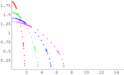
Figure 2: Threshold masses vs. charge density $\lambda$ for black D3-branes having various values of mass density $M$. Extremal values of the charge density are $\lambda_{\rm max}=M/\sqrt{2}\simeq 3.5,\,7.1,\,10.6,\,14.1$, and critical values corresponding to $b_{\rm cr}=1/2$ are $\lambda_{\rm cr}=\sqrt{6}M/7\simeq 1.8,\,3.5,\,5.3,\,7.0$ for $M=5,\,10,\,15,\,20$, respectively.

Now let us consider the extremal black D3-brane, i.e., $k\rightarrow 0$ and $\mu$ (or, $b$) $\rightarrow\infty$ with $kb$ ($\simeq ke^{2\mu}/4$) $=M/4\equiv c$ fixed. The extremal black D3-brane is expected to be stable since they correspond to the BPS ground state in string theory. Our numerical result obtained up to $q\simeq 0.93$ (i.e., $b\simeq 10$) above also seems to indicate that there would not appear instability mode when we continue our analysis further up to the extremal point $q=1$. However, $b\simeq 10$ is still small compared to $b\simeq\infty$, and our analysis based on rescaled variables is not appropriate to the case of extremal limit. In particular, the initial data in Eqs. (31) and (32) cannot be kept small as $b\rightarrow\infty$. Thus we study the extremal case separately. By recovering the parameter $k$ and taking the extremal limit in Eqs. (26) and (27), perturbation equations for the extremal $D3$-brane are given by

$$\varphi^{\prime\prime}+\frac{r^{3}}{P}\bigg{[}5c^{4}m^{2}+5r^{14}\Big{(}-7+m^{2}r^{2}\Big{)}+5c^{3}r^{2}\Big{(}3+4m^{2}r^{2}\Big{)}+cr^{10}\Big{(}37+20m^{2}r^{2}\Big{)}$$

$$+3c^{2}r^{6}\Big{(}21+10m^{2}r^{2}\Big{)}\bigg{]}\varphi^{\prime}-\frac{m^{2}(c+r^{4})^{2}}{P}\bigg{[}c^{3}m^{2}+r^{10}\Big{(}-7+m^{2}r^{2}\Big{)}+3cr^{6}\Big{(}4+m^{2}r^{2}\Big{)}$$

$$+c^{2}r^{2}\Big{(}11+3m^{2}r^{2}\Big{)}\bigg{]}\varphi-\frac{2cr^{5}}{P}\bigg{[}5c^{2}+34cr^{4}-7r^{8}\bigg{]}\psi^{\prime}-\frac{2cr^{2}}{P}\bigg{[}11c^{3}m^{2}-7m^{2}r^{12}$$

$$+c^{2}r^{2}\Big{(}16+15m^{2}r^{2}\Big{)}+cr^{6}\Big{(}80-3m^{2}r^{2}\Big{)}\bigg{]}\psi=0$$ (58)

and

$$\psi^{\prime\prime}+\frac{r^{3}}{P}\bigg{[}5c^{4}m^{2}+r^{14}\Big{(}-49+5m^{2}r^{2}\Big{)}+c^{3}r^{2}\Big{(}-7+20m^{2}r^{2}\Big{)}+cr^{10}\Big{(}187+20m^{2}r^{2}\Big{)}$$

$$+c^{2}r^{6}\Big{(}13+30m^{2}r^{2}\Big{)}\bigg{]}\psi^{\prime}-\frac{1}{P}\bigg{[}c^{5}m^{4}+m^{2}r^{18}\Big{(}7+m^{2}r^{2}\Big{)}+c^{4}m^{2}r^{2}\Big{(}21+5m^{2}r^{2}\Big{)}$$

$$+cr^{12}\Big{(}-384-46m^{2}r^{2}+5m^{4}r^{4}\Big{)}+2c^{2}r^{8}\Big{(}16-46m^{2}r^{2}+5m^{4}r^{4}\Big{)}$$

$$+2c^{3}r^{4}\Big{(}16-9m^{2}r^{2}+5m^{4}r^{4}\Big{)}\bigg{]}\psi-\frac{2r^{5}}{P}\bigg{[}-6c^{3}+17c^{2}r^{4}-12cr^{8}+r^{12}\bigg{]}\varphi^{\prime}$$

$$-\frac{2m^{2}r^{2}}{P}\Big{(}c+r^{4}\Big{)}^{2}\left(6c^{2}-11cr^{4}+r^{8}\right)\varphi=0,$$ (59)

where

$$P(r)=r^{4}\Big{(}c+r^{4}\Big{)}\Big{[}c^{3}m^{2}+r^{10}\Big{(}-7+m^{2}r^{2}\Big{)}+cr^{6}\Big{(}14+3m^{2}r^{2}\Big{)}+c^{2}r^{2}\Big{(}1+3m^{2}r^{2}\Big{)}\Big{]},$$ (60)

and $m$ and $r$ are all dimensionful variables.

Differently from other extremal $p$-brane cases in Ref. Hirayama:2002hn , these equations at the extremal point are not decoupled. Repeating similar analysis as in the cases of non-extremal black $D3$-branes, for given mass density $M$ (or, $c$) we have checked for various values of $m$, but found no regular solution. It confirms that the extremal $D3$-brane is stable, at least under $s$-wave perturbations classically.

IV Conclusions

To conclude, we have investigated the classical stability of black $D3$-branes in the type IIB supergravity under small perturbations. For $s$-wave perturbations it turns out that black $D3$-branes are unstable when they have small charge density. As the charge density increases for a given mass density, however, the instability decreases down to zero at a certain value of the extremality parameter (i.e., $q_{\rm cr}\simeq 0.49$), and then black $D3$-branes become stable all the way down to the extremal point. It has also been shown that such critical value at which its stability behavior changes agrees very well with the predicted one by the thermodynamic stability behavior of the same system through the Gubser-Mitra conjecture. Therefore, although the generalization of Reall’s proof for the GM conjecture Reall:2001ag to the case of black $D3$-branes seems to be non-trivial as explained before, our direct comparison confirms that the GM conjecture presumably holds to this case as well.

The peculiar property in this theory that the five-form field strength should be self-dual is imposed for linearized perturbations as an additional constraint on the solution space. Interestingly, however, it turned out that, for $s$-wave perturbations, such constraint is automatically satisfied since this constraint equation is precisely equal to one of linearized equations for the gauge field. It should also be pointed out that the $s$-wave instability for black $D3$-branes involves a non-vanishing gauge field fluctuation. This property differs from other cases of magnetically charged black $p$-branes studied in Refs. Gregory:1994bj ; Hirayama:2002hn where allowed $s$-wave unstable solutions are for fluctuations of dilaton and gravitational fields only with the gauge field frozen. Although our stability analysis described in this paper is restricted to $s$-wave perturbations so far, we expect that the essential stability behavior of black $D3$-branes would not change even if we consider non-$s$-wave perturbations further. It follows because the strongest instability is expected to be carried by $s$-wave perturbations Gregory:1994bj .

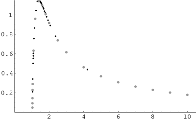
Figure 3: Threshold masses with respect to the horizon radius for a given charge density $\lambda=2\sqrt{2}$. Black dots denote our result and gray dots that of Ref. Gubser:2002yi . $r_{\scriptscriptstyle{H}}=0$ corresponds to the extremal $D3$-brane, and the critical horizon radius is $r_{\scriptscriptstyle{H}{\rm cr}}=(2/\sqrt{3})^{1/4}\simeq 1.04$.

Now let us compare our result with that of Ref. Gubser:2002yi obtained by using the notion of universality classes. Since the gauge field is frozen in the dimensionally reduced action in Ref. Gubser:2002yi , it is of interest to see how this difference in the stability analysis affects to the result. In Fig. 3, by using Eq. (57) and the relation between $b$ and the horizon radius given by

$$r_{\scriptscriptstyle{H}}=\left(\lambda/\sqrt{2(n-1)b(b+1)}\right)^{1/(n-1)},$$ (61)

the threshold mass in our result is plotted with respect to the horizon radius for a given charge density (e.g., $\lambda=2\sqrt{2}$) together with that in Ref. Gubser:2002yi . Here $r_{\scriptscriptstyle{H}}=0$ corresponds to the extremal $D3$-brane, and the critical horizon radius at which the instability sets on (i.e., $b_{\rm cr}=1/2$) is expected to be $r_{\scriptscriptstyle{H}{\rm cr}}=(2/\sqrt{3})^{1/4}\simeq 1.04$. Since the non-vanishing gauge fluctuation is proportional to the charge density for small charge, we expect that the assumption of frozen gauge fluctuation in Ref. Gubser:2002yi might be fine when the charge density of black $D3$-branes is small compared to the mass density. Thus threshold masses in two methods probably agree very well at least for large horizon radii as can be seen in Fig. 3. Indeed $r_{\scriptscriptstyle{H}}=1.6$ corresponds to $q\simeq 0.1$ already. Interestingly, however, Fig. 3 shows that both results are still in very good agreement even for horizon radii near the critical value $r_{\scriptscriptstyle{H}}\simeq 1.04$ (i.e., $q\simeq 0.49$). Thus we see that the approximation $\delta{\mathbf{F}}=0$ taken in Ref. Gubser:2002yi does not change the results much even for rather “strongly” charged branes.

Appendix A Linearized perturbation equations

For $s$-wave perturbations in the form of Eqs. (19) and (24) without imposing $\zeta=\eta=0$, the linearized equations in Eqs. (13) and (14) can be written in components as follows:

($tt$)-component:

$$U\varphi^{\prime\prime}+\frac{U}{2}\left(\ln r^{2n}U^{3}W^{-2}\right)^{\prime}\varphi^{\prime}+\left[U^{\prime\prime}+\frac{U^{\prime}}{2}\left(\ln r^{2n}W^{-2}\right)^{\prime}-\frac{\lambda^{2}W^{n}}{2r^{2n}}-\frac{m^{2}}{W}\right]\varphi$$

$$-\frac{U^{\prime}}{2}\psi^{\prime}-\left[U^{\prime\prime}+\frac{U^{\prime}}{2}\left(\ln r^{2n}W^{-2}\right)^{\prime}-\frac{\lambda^{2}W^{n}}{2r^{2n}}\right]\psi+\frac{U^{\prime}}{2}n\chi^{\prime}+\frac{\lambda^{2}W^{n}}{2r^{2n}}n\chi$$

$$+(n-2)\frac{U^{\prime}}{2}\rho^{\prime}+(n-2)\frac{\lambda^{2}W^{n}}{2r^{2n}}\rho+\frac{U^{\prime}}{2}\zeta^{\prime}+\frac{\lambda^{2}W^{n}}{2r^{2n}}\zeta+\frac{mU^{\prime}}{WU}\eta-\frac{\lambda W^{n}}{r^{2n}}Q=0$$ (62)

($rr$)-component:

$$U\left[\varphi^{\prime\prime}+n\chi^{\prime\prime}+(n-2)\rho^{\prime\prime}+\zeta^{\prime\prime}\right]-\frac{U}{2}\left(\ln r^{2n}UW^{-2}\right)^{\prime}\psi^{\prime}-\left(\frac{\lambda^{2}W^{n}}{2r^{2n}}+\frac{m^{2}}{W}\right)\psi$$

$$+\frac{3U^{\prime}}{2}\varphi^{\prime}+\frac{\lambda^{2}W^{n}}{2r^{2n}}\varphi+\frac{U}{2}\left(\ln r^{4}UW^{-2}\right)^{\prime}n\chi^{\prime}+\frac{\lambda^{2}W^{n}}{2r^{2n}}n\chi+(n-2)\frac{U}{2}\left(\ln UW^{2}\right)^{\prime}\rho^{\prime}$$

$$+(n-2)\frac{\lambda^{2}W^{n}}{2r^{2n}}\rho+\frac{U}{2}\left(\ln UW^{2}\right)^{\prime}\zeta^{\prime}+\frac{\lambda^{2}W^{n}}{2r^{2n}}\zeta+\frac{m}{W}\left(2\eta^{\prime}-\frac{U^{\prime}}{U}\eta\right)-\frac{\lambda W^{n}}{r^{2n}}Q=0$$ (63)

($\theta\theta$)-component:

$$U\chi^{\prime\prime}+\frac{U}{2}\left(\ln r^{4n}U^{2}W^{-n-2}\right)^{\prime}\chi^{\prime}+\Bigg{[}U\frac{\left(r^{2}W^{-1}\right)^{\prime\prime}}{r^{2}W^{-1}}+\frac{U}{2}\left(\ln r^{2}W^{-1}\right)^{\prime}\left(\ln r^{2(n-2)}U^{2}\right)^{\prime}$$

$$-(n-2)\frac{\lambda^{2}W^{n}}{2r^{2n}}-\frac{m^{2}}{W}\Bigg{]}\chi+\frac{U}{2}\left(\ln r^{2}W^{-1}\right)^{\prime}\varphi^{\prime}-\frac{\lambda^{2}W^{n}}{2r^{2n}}\varphi-\frac{U}{2}\left(\ln r^{2}W^{-1}\right)^{\prime}\psi^{\prime}$$

$$-\Bigg{[}U\frac{\left(r^{2}W^{-1}\right)^{\prime\prime}}{r^{2}W^{-1}}+\frac{U}{2}\left(\ln r^{2}W^{-1}\right)^{\prime}\left(\ln r^{2(n-2)}U^{2}\right)^{\prime}+\frac{\lambda^{2}W^{n}}{2r^{2n}}\Bigg{]}\psi+(n-2)\frac{U}{2}\left(\ln r^{2}W^{-1}\right)^{\prime}\rho^{\prime}$$

$$-(n-2)\frac{\lambda^{2}W^{n}}{2r^{2n}}\rho+\frac{U}{2}\left(\ln r^{2}W^{-1}\right)^{\prime}\zeta^{\prime}-\frac{\lambda^{2}W^{n}}{2r^{2n}}\zeta+\frac{m}{W}\left(\ln r^{2}W^{-1}\right)^{\prime}\eta+\frac{\lambda W^{n}}{r^{2n}}Q=0$$ (64)

($z^{i}=z^{j}$)-component:

$$U\rho^{\prime\prime}+\frac{U}{2}\left(\ln r^{2n}U^{2}W^{n-4}\right)^{\prime}\rho^{\prime}+\Bigg{[}U\frac{W^{\prime\prime}}{W}+\frac{U}{2}\frac{W^{\prime}}{W}\left(\ln r^{2n}U^{2}W^{-4}\right)^{\prime}+(n-4)\frac{\lambda^{2}W^{n}}{2r^{2n}}-\frac{m^{2}}{W}\Bigg{]}\rho$$

$$+\frac{U}{2}\frac{W^{\prime}}{W}\varphi^{\prime}+\frac{\lambda^{2}W^{n}}{2r^{2n}}\varphi-\frac{U}{2}\frac{W^{\prime}}{W}\psi^{\prime}-\left[U\frac{W^{\prime\prime}}{W}+\frac{U}{2}\frac{W^{\prime}}{W}\left(\ln r^{2n}U^{2}W^{-4}\right)^{\prime}-\frac{\lambda^{2}W^{n}}{2r^{2n}}\right]\psi$$

$$+\frac{U}{2}\frac{W^{\prime}}{W}n\chi^{\prime}+\frac{\lambda^{2}W^{n}}{2r^{2n}}n\chi+\frac{U}{2}\frac{W^{\prime}}{W}\zeta^{\prime}+\frac{\lambda^{2}W^{n}}{2r^{2n}}\zeta+\frac{m}{W}\frac{W^{\prime}}{W}\eta-\frac{\lambda W^{n}}{r^{2n}}Q=0$$ (65)

($rz^{i}$)-component:

$$U\left[\varphi^{\prime}+n\chi^{\prime}+(n-3)\rho^{\prime}\right]+\frac{U}{2}\left(\ln UW^{-1}\right)^{\prime}\varphi-\frac{U}{2}\left(\ln r^{2n}UW^{-3}\right)^{\prime}\psi$$

$$+\frac{U}{2}\left(\ln r^{2}W^{-2}\right)^{\prime}n\chi+\frac{1}{m}\left[U\frac{W^{\prime\prime}}{W}+\frac{U}{2}\frac{W^{\prime}}{W}\left(\ln r^{2n}U^{2}W^{-4}\right)^{\prime}-\frac{\lambda^{2}W^{n}}{r^{2n}}\right]\eta=0$$ (66)

($z^{i}\not=z^{j}$)-component:

$$U\zeta^{\prime\prime}+\frac{U}{2}\left(\ln r^{2n}U^{2}W^{-2}\right)^{\prime}\zeta^{\prime}+\left[U\frac{W^{\prime\prime}}{W}+\frac{U}{2}\frac{W^{\prime}}{W}\left(\ln r^{2n}U^{2}W^{-4}\right)^{\prime}-\frac{\lambda^{2}W^{n}}{r^{2n}}\right]\zeta$$

$$+\frac{m}{W}\left[2\eta^{\prime}+\left(\ln r^{2n}W^{-4}\right)^{\prime}\eta\right]-\frac{m^{2}}{W}\left[\varphi+\psi+n\chi+(n-4)\rho\right]=0$$ (67)

$\delta F$:

$$\lambda\left[\varphi+\psi+(n-2)\rho-n\chi+\zeta\right]-2Q = 0$$ (68)

$$\lambda\left[\varphi^{\prime}+\psi^{\prime}+(n-2)\rho^{\prime}-n\chi^{\prime}+\zeta^{\prime}\right]-2Q^{\prime} = 0$$ (69)

Two non-trivial components of the equation $\nabla_{M}h^{MN}=\frac{1}{2}\nabla^{N}h$ can be written as

($r$)-component:

$$U\left[\varphi^{\prime}-\psi^{\prime}+n\chi^{\prime}+(n-2)\rho^{\prime}+\zeta^{\prime}\right]+U^{\prime}\varphi-U\left(\ln r^{2n}UW^{-2}\right)^{\prime}\psi$$

$$+U\left(\ln r^{2}W^{-1}\right)^{\prime}n\chi+U\frac{W^{\prime}}{W}\left[(n-2)\rho+\zeta\right]+\frac{2m}{W}\eta=0$$ (70)

($z^{i}$)-component:

$$m\left[\varphi+\psi+n\chi+(n-4)\rho-\zeta\right]-2\eta^{\prime}-\left(\ln r^{2n}W^{-2}\right)^{\prime}\eta=0$$ (71)

Note that Eqs. (66) and (67) do not contain the function $Q(r)$, and also that they are related to Eqs. (70) and (71) as

$$m(\tilde{\ref{leomri}}) = \frac{m}{2}(\tilde{\ref{TGr}})+\frac{U}{2}(\tilde{\ref{TGi}})^{\prime}-\frac{mU}{2}\frac{W^{\prime}}{W}\left[\varphi-\psi+n\chi+(n-2)\rho\right]$$ (72)

$$+U\eta^{\prime\prime}+\frac{U}{2}\left(\ln r^{2n}W^{-2}\right)^{\prime}\eta^{\prime}+\Bigg{[}\frac{U}{2}\frac{W^{\prime}}{W}\left(\ln r^{2n}U^{2}W^{-2}\right)^{\prime}-n\frac{U}{r^{2}}-\frac{\lambda^{2}W^{n}}{r^{2n}}$$

$$-\frac{m^{2}}{W}\Bigg{]}\eta-\frac{mU}{2}\frac{W^{\prime}}{W}\zeta$$

$$(\tilde{\ref{leomiNj}}) = -\frac{m}{W}(\tilde{\ref{TGi}})+U\zeta^{\prime\prime}+\frac{U}{2}\left(\ln r^{2n}U^{2}W^{-2}\right)^{\prime}\zeta^{\prime}+\Bigg{[}U\frac{W^{\prime\prime}}{W}$$ (73)

$$+\frac{U}{2}\frac{W^{\prime}}{W}\left(\ln r^{2n}U^{2}W^{-4}\right)^{\prime}-\frac{\lambda^{2}W^{n}}{r^{2n}}-\frac{m^{2}}{W}\Bigg{]}\zeta-\frac{2m}{W}\frac{W^{\prime}}{W}\eta,$$

where $(\tilde{A}l)$ with $l=5,6,8,9$ denotes the left hand side of Eq. ($Al$). Thus one finds that in the Reall gauge (i.e., $\zeta=\eta=0$) the linearized perturbation equation Eq. (67) becomes equivalent to the $z^{i}$-component of the transverse gauge Eq. (71). As can be seen in Eq. (72), however, Eq. (66) differs from the $r$-component of the transverse gauge Eq. (70) as the black brane gets charged (i.e., $W^{\prime}\not=0$). This property is different from the cases studied in Refs. Hirayama:2002hn ; Reall:2001ag where some of linearized perturbation equations in the Reall gauge become exactly equal to the transverse gauge.

Appendix B Perturbation equations for the $D3$-brane

For black $D3$-branes (i.e., $n=D/2=p+2=5$), the linearized perturbation equations above in the Reall gauge $\zeta=\eta=0$ become

($tt$)-component:

$$\left(1-\frac{1}{r^{4}}\right)\varphi^{\prime\prime}+\frac{5r^{4}+6b+1}{r^{5}(1+b/r^{4})}\varphi^{\prime}-\frac{m^{2}(r^{12}+3br^{8}+3b^{2}r^{4}+b^{3})-4b(b+1)r^{2}}{r^{12}(1+b/r^{4})^{2}}\varphi$$

$$-\frac{(b+2)r^{4}+b}{r^{9}(1+b/r^{4})}\psi^{\prime}-\frac{4b(b+1)}{r^{10}(1+b/r^{4})^{2}}\psi+\frac{(b+2)r^{4}+b}{r^{9}(1+b/r^{4})}5\chi^{\prime}+\frac{4b(b+1)}{r^{10}(1+b/r^{4})^{2}}5\chi$$

$$+\frac{(b+2)r^{4}+b}{r^{9}(1+b/r^{4})}3\rho^{\prime}+\frac{4b(b+1)}{r^{10}(1+b/r^{4})^{2}}3\rho-\frac{2\sqrt{2b(b+1)}}{r^{10}(1+b/r^{4})^{2}}Q=0$$ (74)

($rr$)-component:

$$\left(1-\frac{1}{r^{4}}\right)\left[\varphi^{\prime\prime}+5\chi^{\prime\prime}+3\rho^{\prime\prime}\right]-\frac{5r^{8}+(4b-3)r^{4}-2b}{r^{9}(b+1/r^{4})}\psi^{\prime}-\frac{m^{2}(r^{4}+b)^{3}+4b(b+1)r^{2}}{r^{12}(1+b/r^{4})^{2}}\psi$$

$$+3\frac{(b+2)r^{4}+b}{r^{9}(1+b/r^{4})}\varphi^{\prime}+\frac{4b(b+1)}{r^{10}(1+b/r^{4})^{2}}\varphi+\frac{2r^{8}+br^{4}+b}{r^{9}(1+b/r^{4})}5\chi^{\prime}+\frac{4b(b+1)}{r^{10}(1+b/r^{4})^{2}}5\chi$$

$$+\frac{(3b+2)r^{4}-b}{r^{9}(1+b/r^{4})}3\rho^{\prime}+\frac{4b(b+1)}{r^{10}(1+b/r^{4})^{2}}3\rho-\frac{2\sqrt{2b(b+1)}}{r^{10}(1+b/r^{4})^{2}}Q=0$$ (75)

($\theta\theta$)-component:

$$\left(1-\frac{1}{r^{4}}\right)\chi^{\prime\prime}+\frac{10r^{8}+(5b-6)r^{4}-b}{r^{9}(1+b/r^{4})}\chi^{\prime}-\frac{1}{r^{12}(1+b/r^{4})^{2}}\Bigg{[}m^{2}(r^{12}+3br^{8}+3b^{2}r^{4}+b^{3})$$

$$-8r^{10}-16br^{6}+4b(3b+5)r^{2}\Bigg{]}\chi+\frac{1-1/r^{4}}{r(1+b/r^{4})}\varphi^{\prime}-\frac{4b(b+1)}{r^{10}(1+b/r^{4})^{2}}\varphi-\frac{1-1/r^{4}}{r(1+b/r^{4})}\psi^{\prime}$$

$$-4\frac{2r^{8}+4br^{4}+b(b-1)}{r^{10}(1+b/r^{4})^{2}}\psi+\frac{1-1/r^{4}}{r(1+b/r^{4})}3\rho^{\prime}-\frac{4b(b+1)}{r^{10}(1+b/r^{4})^{2}}3\rho$$

$$+\frac{2\sqrt{2b(b+1)}}{r^{10}(1+b/r^{4})^{2}}Q=0$$ (76)

($z^{i}=z^{j}$)-component:

$$\left(1-\frac{1}{r^{4}}\right)\rho^{\prime\prime}+\frac{5r^{8}+(8b-1)r^{4}-4b}{r^{9}(1+b/r^{4})}\rho^{\prime}-\frac{m^{2}(r^{12}+3br^{8}+3b^{2}r^{4}+b^{3})-12b(b+1)r^{2}}{r^{12}(1+b/r^{4})^{2}}\rho$$

$$+b\frac{1-1/r^{4}}{r^{5}(1+b/r^{4})}\varphi^{\prime}+\frac{4b(b+1)}{r^{10}(1+b/r^{4})^{2}}\varphi-b\frac{1-1/r^{4}}{r^{5}(1+b/r^{4})}\psi^{\prime}-\frac{4b(b+1)}{r^{10}(1+b/r^{4})^{2}}\psi$$

$$+b\frac{1-1/r^{4}}{r^{5}(1+b/r^{4})}5\chi^{\prime}+\frac{4b(b+1)}{r^{10}(1+b/r^{4})^{2}}5\chi-\frac{2\sqrt{2b(b+1)}}{r^{10}(1+b/r^{4})^{2}}Q=0$$ (77)

($rz^{i}$)-component:

$$\varphi^{\prime}+5\chi^{\prime}+2\rho^{\prime}+\frac{2}{r^{5}(1-1/r^{4})}\varphi$$

$$-\frac{5r^{8}+3(b-1)r^{4}-b}{r^{9}(1-1/r^{4})(1+b/r^{4})}\psi+\frac{r^{4}-b}{r^{5}(1+b/r^{4})}5\chi=0$$ (78)

($z^{i}\not=z^{j}$)-component:

$$\varphi+\psi+5\chi+\rho=0$$ (79)

$\delta F$:

$$\lambda\left[\varphi+\psi+3\rho-5\chi\right]-2Q=0$$ (80)

Here $b=\sinh^{2}\mu$ and we set $k=1$.

References

• (1) A. Ishibashi and H. Kodama, Prog. Theor. Phys.  110, 901 (2003) [arXiv:hep-th/0305185].
• (2) R. Gregory and R. Laflamme, Phys. Rev. Lett. 70, (1993) 2837.
• (3) R. Gregory and R. Laflamme, Nucl. Phys. B 428, 399 (1994) [arXiv:hep-th/9404071].
• (4) R. Gregory and R. Laflamme, Phys. Rev. D 51, 305 (1995) [arXiv:hep-th/9410050].
• (5) T. Hirayama and G. Kang, Phys. Rev. D 64, 064010 (2001) [arXiv:hep-th/0104213].
• (6) R. Gregory, Class. Quant. Grav.  17, L125 (2000) [arXiv:hep-th/0004101].
• (7) G. Kang, Proceedings of the 11th Workshop on General Relativity and Gravitation held at Tokyo, Japan, Jan. 9-12, 2002, arXiv:hep-th/0202147; G. Kang and Y. Lee;“Lower Dimensional Black Strings/Branes Are Stable,” preprint KIAS-P03063 (2003).
• (8) T. Hirayama, G. Kang and Y. Lee, Phys. Rev. D 67, 024007 (2003) [arXiv:hep-th/0209181].
• (9) M. J. Duff, H. Lu and C. N. Pope, Phys. Lett. B 382, 73 (1996) [arXiv:hep-th/9604052].
• (10) S. S. Gubser and I. Mitra, arXiv:hep-th/0009126; JHEP 0108, 018 (2001) [arXiv:hep-th/0011127].
• (11) H. S. Reall, Phys. Rev. D 64, 044005 (2001) [arXiv:hep-th/0104071].
• (12) T. Prestidge, Phys. Rev. D 61 (2000) 084002 [arXiv:hep-th/9907163]; J. P. Gregory and S. F. Ross, Phys. Rev. D 64, 124006 (2001) [arXiv:hep-th/0106220].
• (13) S. S. Gubser and A. Ozakin, JHEP 0305, 010 (2003) [arXiv:hep-th/0301002].