The whole idea of holography as put forward by Gerard ’t Hooft assumes that data on a boundary determine physics in the volume. This corresponds to a Dirichlet problem for euclidean signature, or to a Goursat (characteristic) problem in the lorentzian setting. Is this last aspect of the problem that is explored here for Ricci flat spaces with vanishing cosmological constant.

1 Introduction

Ever since its inception, the whole idea of holography (cf. [22] [21]) stand as one of the most original and mysterious suggestions ever made in fundamental physics.

From a certain abstract viewpoint, it certainly includes at least two facts .

The first one is that it should be possible to recover volume information on the physical fields from data given on a certain surface, namely the boundary of the volume. That is, fields in the volume do not obey an ordinary Cauchy problem (for which also derivatives of the field at the boundary would also be needed), but rather a degenerate one, in which the derivative cannot be imposed independently. This happens both for timelike and null initial surfaces.

Second, the volume symmetries (i.e. diffeomorphism invariance) should guarantee conformal (or at least scale) invariance on the boundary.

In addition, although the main thrust of the holographic principle lies in its application to the fundamental degrees of freedom of quantum gravity, it seems sensible to assume that there is at least a regime in the space of parameters in which these properties are true already at a classical level.

Holography for vanishing cosmological constant remains quite mysterious to this day, and in any case is strongly suspected to be realized (if at all) in a subtler from than a Conformal Field Theory (CFT); indeed Witten (cf. [24]) coined the name Structure X to refer to it(cf. also [3]).

When the cosmological constant is negative, as in the conjectured duality of Maldacena ( [18]), the mapping takes place because the conformal boundary in the Penrose sense ([19]) of Anti de Sitter (AdS) is timelike, so that data on this boundary determine the interior dynamics, with some qualifications ([13][23]). Curiously enough the ordinary Cauchy problem is not well posed in spaces of constant negative curvature, unless some extra physical hypothesis are assumed (cf. the discussion in [4]). Of course, this rather vague ideas can be implemented in a precise way in the supersymmetric context of $IIB$ strings in $AdS_{5}\times S_{5}$ with $N$ units of Ramond-Ramond (RR) flux. In this case, the conformal group is realized as an isometry group in the bulk, so that the boundary theory must be conformal ($\beta=0$).

Recently we have pointed out some indications of holographic behavior in a rather general class of Ricci flat string backgrounds with vanishing cosmological constant ([1]) of the form

$$M_{10}\equiv A_{6}\times C_{4}$$ (1)

where $C_{4}$ is an internal compact manifold, and $A_{6}$ will be denoted by the name ambient space. No RR backgrounds are excited, so that this background is universal. In this ambient space lives a codimension two euclidean four-manifold, which will be interpreted as the spacetime $M_{4}\subset A_{6}$. The spacetime coordinates will be denoted by $y^{i}\equiv\vec{y}$ and its metric by $g_{ij}dy^{i}dy^{j}$; whereas the extra two coordinates of the ambient space by $\rho\in\mathbb{R}^{+}$ and $T\in\mathbb{R}^{+}$, where $\rho$ is spacelike and $T$ timelike. There is then a natural five-dimensional boundary defined in this patch by

$$\partial A_{6}\equiv\{\rho=0\}$$ (2)

It is worth remarking that this boundary is null, and it is then essentially equivalent to Penrose’s conformal boundary, which is known to play a central rôle in holography.

An important fact worth remembering is that the conformal boundary of a (conformal) boundary does not necessarily vanish.

There are then two conformal boundaries in this setting: the finite one at $\rho=0$, which is also a mathematical boundary located at finite distance, and the usual conformal boundary at infinity, the appropiate $\mathcal{J}^{+}$.

It will become clear in the sequel that in many cases we will be able to interpret the whole space as the curved interior of some light-cone, which itself represents the boundary.

Those spaces (from now on we shall work in arbitrary dimension $d=n+2$, because most results are quite general) enjoy a homothecy that is, a conformal Killing vector (CKV) with constant conformal factor, which acts on the metric through a scale transformation

$$\pounds(k)g_{\alpha\beta}=2g_{\alpha\beta}$$ (3)

Canonical coordinates can be chosen such that the whole ambient space metric reads:

$$ds^{2}=\frac{T^{2}}{l^{2}}ds^{2}(y,\rho)+\rho dT^{2}+Td\rho dT$$ (4)

The CKV itself is then related to the preferred timelike coordinate through

$$k\equiv T\,\frac{\partial}{\partial T}$$ (5)

where the metric reduces on the null codimension-one hypersurface $\rho=0$ to the (riemannian) $n-$dimensional spacetime metric (up to a rescaling):

$$ds^{2}(y,\rho=0)=\frac{T^{2}}{l^{2}}g_{ij}(y)dy^{i}dy^{j}.$$ (6)

The norm of the CKV is given by

$$k^{2}=\rho T^{2}$$ (7)

The boundary then has an invariant characterization as a Killing horizon, the set of points where the norm of the CKV vanishes.

Under Weyl rescalings of the metric (4),

$$g_{\alpha\beta}\rightarrow\hat{g}_{\alpha\beta}\equiv\Omega^{2}(T,\rho,y)g_{\alpha\beta}$$ (8)

the same vector $k$ given by (5) remains a CKV, because

$$\pounds(k)\hat{g}_{\mu\nu}=\bigg{(}2+\frac{\partial\log{\Omega}}{\partial\log{T}}\bigg{)}\hat{g}_{\mu\nu}$$ (9)

and its norm changes by a conformal factor

$$k^{2}=\Omega^{2}\rho T^{2}$$ (10)

This means that the whole setup is conformally invariant. In particular, the interpretation of the boundary as the Killing horizon of the CKV survives Weyl rescalings.

The purpose of the present paper is to study the interplay bulk/boundary in this framework. One of the main characteristics is the fact that the finite boundary (that is, the one at $\rho=0$) is precisely located at finite distance, in spite of being also a conformal boundary; as we have already said there is always in addition the boundary at infinity , $\mathcal{J}^{+}$ as well, which is infinitely far away as usual. We shall mainly be concerned with the appropiate generalizations of the bulk-boundary Green functions, as well as with the symmetries of the finite boundary action. In this paper we assume that all relevant curvatures are small enough so that a (super)gravity treatment is a useful first approximation.

2 The simplest example: the Milne Universe

The whole idea of the present approach implicity assumes that the ordinary Cauchy problem has been replaced by a characteristic one (cf. [10]), usually called Goursat’s problem in the mathematical literature. In the former, Cauchy data on a spacelike surface (such as $t=const$ in flat space) are given. This means, for the wave equation, giving the field and the normal (time) derivative of it in the initial surface, and the solution is then fully determined in the causal development of the Cauchy surface. The characteristic problem, on the other hand, specifies half of the data (i.e., the field itself) on a characteristic surface of the hyperbolic equation, such as the light cones in the flat case. The solution is then fully determined in the inside of the cone only. Curiously enough, if we consider the inside of the light cone as a mildly singular manifold the ordinary Cauchy problem is delicate.

As a simple example, where however, all the ideas get illustrated, let us think for a moment on the forward light cones $N_{+}$ on flat (n+2)-dimensional space, the simplest possible background. The inside of the forward light cone is what is usually denoted by Milne’s Universe ([6]). The general situation can be studied with few modifications .

There are then two boundaries in our space (cf. Figure). One is the finite conformal boundary, i.e., the future light cone of the origin, $N_{+}(0)$. The other one is the future null infinity, $\mathcal{J}^{+}$. The Penrose diagram of the Milne universe corresponds thus to the portion of Minkowski space shown in the figure.

The starting point is then the flat metric

$$ds^{2}=\eta_{\mu\nu}dx^{\mu}dx^{\nu}=(dx^{0})^{2}-d\vec{x}^{2}$$ (11)

($x^{i}=(x^{1}\ldots x^{n+1})$ and we employ $x^{0}=t$ indistinctly). The equation of the light cones is

$$x_{0}=r\equiv|\vec{x}|$$ (12)

conveying the fact that they are null surfaces themselves, since their normal vector

$$n\equiv(1,n^{i}\equiv\frac{x^{i}}{r})$$ (13)

is null. By the way,these coordinates have nothing to do with the canonical coordinates introduced above. The explicit relationship is

$$T=x_{-}\equiv x_{0}-x_{n+1}$$

$$y^{i}=\frac{lx^{i}}{x_{-}}(i\neq n+1)$$

$$\rho=\frac{x_{\mu}x^{\mu}}{x_{-}^{2}}$$ (14)

Their local structure is $S^{n}\times\mathbb{R}^{+}$, and a point in $N_{+}$ can be specified by $(x_{0},n^{i})$, where $x_{0}\in\mathbb{R}^{+}$ and $\vec{n}^{2}=1$ is a point on the unit n-dimensional sphere, $S_{n}$, that is, a $(n+1)$-dimensional structure. The light cone can be visualized as a $S_{n}$ sphere of radius $x_{0}$.

The induced metric is, however, degenerate (that is, as a matrix it has rank $n$), because the time differential is totally absent from the line element:

$$ds_{+}^{2}=x_{0}^{2}d\Omega_{n}^{2}$$ (15)

where $d\Omega_{n}^{2}$ is the metric on the unit n-sphere, $S_{n}$, which in terms of angular variables reads:

$$d\Omega_{n}^{2}\equiv d\theta_{n}^{2}+\sin{\theta_{n}}^{2}d\theta_{n-1}^{2}+\ldots+\sin{\theta_{n}}^{2}\sin{\theta_{n-1}}^{2}\ldots\sin{\theta_{2}}^{2}d\theta_{1}^{2}$$ (16)

This means that, although singular as a metric on $N_{+}$, the metric is perfectly regular (actually the standard one) as a metric on the n-spheres $t=constant$.

The invariant volume element, however, vanishes, due to the fact that the determinant of the induced metric is zero.

The metric con $N_{+}$ inherits the homothecy giving rise to scale transformations on the metric which now reads $k\equiv x_{0}\partial_{x_{0}}$ and still obeys

$$\pounds(k)g_{\alpha\beta}=2g_{\alpha\beta}$$ (17)

Remarkably enough, the complete set of isometries of the three-dimensional metric (15) includes the full Lorentz group, $SO(1,3)$. Please note that isometries are well-defined, even for singular metrics, through the vanishing Lie-derivative condition $\pounds(k)g_{\mu\nu}=0$, reflecting the invariance of the metric under the corresponding one-parametric group of diffeomorphisms, although of course this is not equivalent to $\nabla_{\mu}k_{\nu}+\nabla_{\nu}k_{\mu}=0$ because the covariant derivative (that is, the Christoffel symbols ) is not well defined owing to the absence of the inverse metric.

The six Killing vectors that generate $SO(1,3)$ are :

$$J_{1}=\cos{\phi}\frac{\partial}{\partial\theta}-\cot{\theta}\sin{\phi}\frac{\partial}{\partial\phi}$$

$$J_{2}=\sin{\phi}\frac{\partial}{\partial\theta}+\cot{\theta}\cos{\phi}\frac{\partial}{\partial\phi}$$

$$J_{3}=\frac{\partial}{\partial\phi}$$

$$K_{1}=-x^{0}\sin{\theta}\sin{\phi}\frac{\partial}{\partial x^{0}}-\cos{\theta}\sin{\phi}\frac{\partial}{\partial\theta}-\frac{\cos{\phi}}{\sin{\theta}}\frac{\partial}{\partial\phi}$$

$$K_{2}=x^{0}\sin{\theta}\cos{\phi}\frac{\partial}{\partial x^{0}}+\cos{\theta}\cos{\phi}\frac{\partial}{\partial\theta}-\frac{\sin{\phi}}{\sin{\theta}}\frac{\partial}{\partial\phi}$$

$$K_{3}=x^{0}\cos{\theta}\frac{\partial}{\partial x^{0}}-\sin{\theta}\frac{\partial}{\partial\theta}$$ (18)

Let us point out, however, that a slight shift in viewpoint uncovers an infinite group of isometries.

The light cone can indeed be considered as the infinite curvature limit of EAdS. (cf. [2]). The exact relationship between cartesian and horospheric coordinates in the infinite curvature limit is:

$$x_{0}=\frac{1}{2z}(y_{T}^{2}+1)$$

$$x_{3}=\frac{1}{2z}(y_{T}^{2}-1)$$

$$x_{T}=\frac{y_{T}}{z}$$ (19)

where the subscript transverse refers to the $(1,2)$ labels: $y_{T}\equiv(y_{1},y_{2})$. It is worth pointing out that the coordinate $z$ has got dimensions of energy, whereas the $y_{T}$ are dimensionless.

Horospheric coordinates then break down when $x_{0}=x_{3}$; that is, when $z=\infty$. The metric of the cone reads now

$$ds^{2}=\frac{dy_{1}^{2}+dy_{2}^{2}}{z^{2}}$$ (20)

It is a simple matter to recover the Killings corresponding to the Lorentz subgroup.

But there are more Killing vectors. First of all, the two translational ones, obvious in these coordinates:

$$P_{1}\equiv\frac{\partial}{\partial y_{1}}$$

$$P_{2}\equiv\frac{\partial}{\partial y_{2}}$$

and some others as well. The fact that there is translation invariance in horospheric coordinates in $N_{+}$ is of great importance in the definition itself of the Green functions.

It is actually possible to give the general solution of the Killing equation in closed form using our horospheric coordinates. Given an arbitrary harmonic function of the two variables $(y_{1},y_{2})$, it is given by:

$$k\equiv(\frac{\partial^{2}}{\partial y_{1}^{2}}f)z\frac{\partial}{\partial z}+(\frac{\partial}{\partial y_{1}}f)\frac{\partial}{\partial y_{1}}-(\frac{\partial}{\partial y_{2}}f)\frac{\partial}{\partial y_{2}}$$ (22)

The finite transformations corresponding to those Killing vectors are:

$$y_{1}\rightarrow y_{1}+\partial_{1}f$$

$$y_{2}\rightarrow y_{2}-\partial_{2}f$$

$$z\rightarrow\sqrt{(1+\partial_{1}\partial_{1}f)^{2}+(\partial_{1}\partial_{2}f)^{2}}$$ (23)

The composition of two succesive transformations characterized by the harmonic functions $f$ and $g$ is equivalent to the function

$$F(f,g)\equiv f(y_{1},y_{2})+g(y_{1}+\partial_{1}f,y_{2}-\partial_{2}f)$$ (24)

The conmutator function is then easily found to be

$$[f,g]=f(y_{1},y_{2})+g(y_{1}+\partial_{1}f,y_{2}-\partial_{2}f)-g(y_{1},y_{2})-f(y_{1}+\partial_{1}g,y_{2}-\partial_{2}g)$$ (25)

It is now clear that the isometry group of the four-dimensional light cone $N_{+}$ is an infinite dimensional group, which includes the Lorentz group as a subgroup.

We find this to be a remarkable situation.

Even more remarkable is the fact that in higher dimension, when the total space gets dimension $d$, say, so that the light cone has dimension $d-1$, and in horospheric coordinates is characterized by $z$ and $\vec{y}\in\mathbb{R}^{d-2}$, in such a way that the metric reads

$$ds^{2}=\frac{d\vec{y}^{2}}{z^{2}},$$ (26)

and the Killing equations are equivalent to

$$\partial_{i}k_{j}+\partial_{j}k_{i}=2\delta_{ij}\xi(\vec{y})$$ (27)

for the total vector

$$k=z\xi(\vec{y})\partial_{z}+\sum_{i=1}^{d-2}k^{i}\partial_{i}$$ (28)

But the equations (27) are precisely the equations for the conformal Kiling vectors of flat $(d-2)$-dimensional space, known to generate the euclidean conformal group, $SO(1,d-1)$, isomorphic to the $d$-dimensional Lorentz group. To be specific ([12]),

$$\xi(\vec{y})\equiv\lambda-2\vec{b}.\vec{y}$$ (29)

and the components on the $y$-directions read:

$$k_{i}=a_{i}+\omega_{ij}y^{j}+\lambda y_{i}+b_{i}y^{2}-2\vec{b}.\vec{y}y_{i}$$ (30)

representing translations ($a$), rotations ($\omega_{(ij)}=0$), scale transformations, $(\lambda)$, and special conformal transformations ($b)$.

To summarize, the isometry group of the light cone at the origin, $N_{+}(0)$, is generically the spacetime Lorentz group except in the four dimensional case, in which it expands to the infinite group we derived above.

Also interesting are those transformations that leave invariant the metric up to a Weyl rescaling (which should include our group as a subgroup). Those are the conformal isometries which in four dimensions span the so called the Newman-Unti (NU) group (cf. [19]), i.e.

$$x^{0}\rightarrow F(x^{0},z,\bar{z})$$

$$z\rightarrow\frac{az+b}{cz+d}$$ (31)

where $z$ is the complex stereographic coordinate of the sphere $S_{2}$, and not the horospheric coordinate. The NU group is also an infinite dimensional extension of the Möbius group. In the appendix we have worked out some illustrative examples.

The Bondi-Metzner-Sachs (BMS) subgroup consists on those transformations which are linear in $x^{0}$.

3 Riesz’ potential in the massless case.

The characteristic problem is much less well-known than the corresponding Cauchy problem. It only makes sense for hyperbolic equations, and then the problem is to determine the solution in a suitable domain of dependence, given the field in a characteristic surface (such as a light cone for the wave or Klein-Gordon equation). Is equivalent to a degenerate Cauchy problem in that the derivative cannot be prescribed arbitrarily; the relationship with the Dirichlet problem of the elliptic euclidean equation is subtle, and will be dealt with (through some elementary examples) in an Appendix. It seems to have been completely solved for the wave equation by d’Adhemar in 1905 (cf.[11]). Indeed, in the book [19] reference is made to the Kirkchhoff-d’Adhemar formula. In general the integrals needed when the classic techniques of Kirkchhoff and Volterra are directly applied are divergent. In one of the last chapters of the classic age of mathematical physics, J. Hadamard introduced the concept of partie finie [15] in order to give a precise recipe to compute them. We shall employ here, however, mainly the equivalent (although somewhat more general) alternative solution elaborated by Riesz [20], and based on analytically continuing integrals depending on a complex parameter in such a way that they are convergent in a particular region of the complex plane, a method which was to become popular among physicists many decades later. The mathematical problems encountered are not unrelated to the ones appearing when a precise meaning is given to the equations of motion in general relativity, or even in classical electrodynamics. Dimensional regularization ([7]) can most likely be employed here as well although we shall not pursue this avenue in this paper.

3.1 Generalities on the characteristic problem

In order to have a first look at the main differences between Goursat’s and Cauchy’s problems, let us consider a scalar field in the interior of the light cone, $C_{+}$, with prescribed values on the cone itself, $N_{+}$ (all this in flat n-dimensional Minkowskian space)

$$\Phi|_{N_{+}}(t=r,\vec{n})=\psi(t,\vec{n})$$ (32)

In ingoing (u) and outgoing (v) null coordinates

$$u\equiv t+r$$

$$v=t-r$$ (33)

the metric reads

$$ds^{2}=dudv-\frac{(u-v)^{2}}{4}d\Omega_{n-2}^{2}$$ (34)

The boundary is now $v=0$, and it can be said that

$$\Phi|_{N_{+}}(u,v=0,\vec{n})=\psi(u,\vec{n})$$ (35)

It is plain that the $\frac{\partial}{\partial u}$ derivative is determined by the boundary condition:

$$\partial_{u}\Phi(u,v=0,\vec{n})=\partial_{u}\psi(u,\vec{n})$$ (36)

but the $\frac{\partial}{\partial v}$ derivative instead is unknown in principle:

$$\partial_{v}\Phi(u,v=0,\vec{n})\equiv f(u,\vec{n})$$ (37)

This is precisely the would-be extra data in a Cauchy problem, the analogous of the normal derivative of the field at the initial surface.

In our case, however, this function $f$ is not arbitrary, but instead it is fully determined in terms of $\psi$ through the wave equation in the cone:

$$4\partial_{u}f-\frac{2n-4}{u}(\partial_{u}\psi-f)-\frac{4}{u^{2}}\Delta_{\vec{n}}\psi=0$$ (38)

(where $\Delta_{\vec{n}}$ is the laplacian on the sphere $S_{n-2}$). The ordinary differential equation that the unknown function $f$ obeys is easily solved:

$$f(u,\vec{n})=\frac{1}{4}u^{-(n-2)/2}\int^{u}\tau^{(n-2)/2}d\tau\big{(}\frac{2n-4}{\tau}\partial_{u}\psi(\tau)+\frac{4}{\tau^{2}}\Delta_{\vec{n}}\psi(\tau)\big{)}$$ (39)

Please note that

$$\partial_{t}\Phi\big{|}_{t=r}=\partial_{u}\psi(u,\vec{n})+f(u,\vec{n})$$ (40)

whereas

$$\partial_{r}\Phi\big{|}_{t=r}=\partial_{u}\psi(u,\vec{n})-f(u,\vec{n})$$ (41)

which are different in general.

3.2 The Generalized Potential of Order $a$.

Let us consider the lorentzian generalization of the Riemann-Liouville integral (cf. Appendix)

$$I^{a}f(x)=\frac{1}{H_{n}(a)}\int_{D^{x}_{S}}f(y)\tau_{xy}^{a-n}dy$$ (42)

where $\tau_{xy}$ is the proper time (geodesic distance) between the points $x$ and $y$, and

$$H_{n}(a)\equiv\pi^{n/2-1}2^{a-1}\Gamma(a/2)\Gamma(\frac{a+2-n}{2})$$ (43)

and $D^{x}_{S}$ is the region bounded by the past light cone of the point $x$, $N_{-}(x)$, and the codimension one hypersurface $S$. This construct satisfies

$$I^{a}I^{b}=I^{a+b}$$

$$\Box I^{a+2}=I^{a}$$ (44)

besides the characteristic property of the Riemann-Liouville integral

$$I^{0}f=f$$ (45)

One can then say in a certain sense that

$$I^{2}=\Box^{-1}$$ (46)

3.3 Stokes’theorem at work

Let us indeed consider the integral over an arbitrary n-dimensional chain $D$

$$I\equiv\int_{D}fd*dg-gd*df=\int_{D}d(vol)(f\Box g-g\Box f)$$ (47)

where the invariant volume element is defined by

$$d(vol)\equiv\sqrt{|g|}dx^{1}\wedge\ldots\wedge dx^{n}$$ (48)

Stokes theorem guarantees that

$$I=\int_{D}d(f*dg-g*df)+dg\wedge*df-df\wedge*dg=\int_{\partial D}(f*dg-g*df)$$ (49)

Let us now consider as $D$ the interior region bounded by two light cones in n-dimensional Minkowski space, one corresponding to the future of the origin $(N_{+}(0)$ which is the characteristic surface), and another one the past light cone of an arbitrary point,$(N_{-}(P)$, where $P\equiv x^{\mu}$.

Figure 1:

Let us now consider the functions $g\equiv\tau_{xy}^{2\lambda}\equiv(x-y)^{2\lambda}$ and $f\equiv\phi(x)$ is the solution we are seeking for, $\Box\phi(x)=0$ and $\phi|_{N_{+}(0)}=\psi$. We then have

$$2\lambda(n+2\lambda-2)\int_{D}\phi(y)(x-y)^{2\lambda-2}=\int_{\partial D}\left(\phi*d\tau_{xy}^{2\lambda}-\tau_{xy}^{2\lambda}*d\phi\right)$$ (50)

The first integral is easily seen to be proportional to the Riemann-Liouville integral

$$I^{2\lambda+n-2}\phi=\frac{1}{H_{n}(n+2\lambda)}\int_{\partial D}\left(\phi*d\tau_{xy}^{2\lambda}-\tau_{xy}^{2\lambda}*d\phi\right)$$ (51)

(where the well-known identity $z\Gamma(z)=\Gamma(1+z)$ has been used).

The main thrust of Riesz approach comes here: the first member tends to $I^{0}\phi=\phi$ (the only instance allowed by dimensional considerations) when

$$\lambda\rightarrow 1-n/2$$ (52)

On the other hand, if we agree in defining the second member trough analytic continuation, it is cleat that for $Re\,\lambda$ large enough the part of the boundary including $N_{-}(P)$ will not contribute, and we are left with the only task of computing the integral over $N_{+}(0)$.

$$\phi(x)=(I^{0}\phi)(x)=\lim_{\lambda\rightarrow 1-\frac{n}{2}}\frac{1}{2^{n+2\lambda-1}\pi^{\frac{n}{2}-1}\Gamma(\lambda+\frac{n}{2})\Gamma(\lambda+1)}\int_{y\in N_{+}(0)}{\left(\phi(y)*d\tau_{xy}^{2\lambda}-\tau_{xy}^{2\lambda}*d\phi(y)\right)}$$ (53)

3.4 The concept of characteristic propagator

The basic equation (53) , after integration by parts, can be expressed as an integral operator of the type

$$\phi(x)=\int_{y\in N_{+}(0)}D_{c}(x,y)\psi(y)$$ (54)

mapping the characteristic data $\psi$ into the bulk solution $\phi$. We shall see in due time that this definition is delicate, because there are cancellations between zeroes and poles which appear only after integration.

Some general properties can be however drawn from the general formula (53). Please note for example that given the fact that if $x\in N_{+}$ $x+a$ does not necessarily belong to $N_{+}$, there is no general reason why the propagator $D_{c}$ ought to depend on the difference $x-y$ only. That is, if for a general function $f$ we call $(T_{a}f)(x)\equiv f(x+a)$ then in order to show that the image of $T_{a}\psi$ is $T_{a}\phi$ we need translation invariance.

There is more in this point than meets the eye, as shall be seen in due course.

Exactly the same argument shows that in our case, the image of the scaled function $(T_{\Omega}\psi)(x)\equiv\psi(\Omega x)$ is $(T_{\Omega}\phi)(x)$, owing to the fact that acting on the first argument

$$D_{c}(\Omega x,y)=\Omega^{2\lambda}D_{c}(x,y)$$ (55)

3.5 Three and four-dimensional examples

One on the main properties of the solution to Goursat’s problem (shared with Cauchy’s problem) is that for even total spacetime dimensions the solution depends only on data defined on the intersection of the past light cone of the point at which the solution is evaluated, with the characteristic. This is the essence of Huyghens’principle, and we shall call the corresponding codimension two surface Huyghens surface ${\cal H}\equiv N_{-}(P)\cap N_{+}(0)$. For odd spacetime dimensions this is not so, and the integrals span the whole codimension one region of the characteristic preceding the Huyghens surface.

Let us be specific in the simplest situations. In a $n=2+1$ dimensional spacetime

$$*d\phi=\frac{\partial\phi}{\partial t}rdr\wedge d\theta+\frac{\partial\phi}{\partial r}rdt\wedge d\theta-\frac{\partial\phi}{\partial\theta}rdt\wedge dr$$ (56)

On the future light cone of the origin, $t=r$ the last term vanishes, yielding ($u=t+r$)

$$*d\phi=2r\frac{\partial\phi}{\partial u}dr\wedge d\theta$$ (57)

Instead of using the coordinate $r$, it is convenient to employ (only to the effect of the computation of the integral) the square of the proper time measured from the point $P\equiv(\bar{x}^{\mu})$, that is

$$R\equiv\tau^{2}=(\bar{x}-x)^{2}=\bar{x}^{2}+2r(\bar{x}_{1}\cos{\theta}+\bar{x}_{2}\sin{\theta}-\bar{x}_{0})$$ (58)

This leaves us with

$$\phi^{(3)}(\bar{x})=\lim_{\lambda\rightarrow-1/2}\int\frac{d\theta}{2\pi}\int_{0}^{\bar{x}^{2}}\Big{[}\psi(R_{\bar{x}},\theta)\lambda R_{\bar{x}}^{\lambda-1}\frac{R_{\bar{x}}-\bar{x}^{2}}{2(\bar{x}_{1}\cos{\theta}+\bar{x}_{2}\sin{\theta}-\bar{x}_{0})}$$

$$-R_{\bar{x}}^{\lambda}\frac{\partial\psi}{\partial u}\frac{R_{\bar{x}}-\bar{x}^{2}}{2(\bar{x}_{1}\cos{\theta}+\bar{x}_{2}\sin{\theta}-\bar{x}_{0})^{2}}\Big{]}dR_{\bar{x}}$$ (59)

Now we can write (we shall suppress the subindex in $R$ unless the equation is prone to confusion)

$$\frac{\partial\psi}{\partial u}=\frac{\partial\psi}{\partial R}(\bar{x}_{1}\cos{\theta}+\bar{x}_{2}\sin{\theta}-\bar{x}_{0})$$ (60)

and performing integration by parts we can reach an expression without derivatives of $\psi$, which for our present purposes is best suited;

$$\phi^{(3)}(\bar{x})=\lim_{\lambda\rightarrow-1/2}\int\frac{d\theta}{2\pi}\frac{1}{2(\bar{x}_{1}\cos{\theta}+\bar{x}_{2}\sin{\theta}-\bar{x}_{0})}\int_{0}^{\bar{x}^{2}}dRR^{\lambda-1}[(1+2\lambda)R-2\bar{x}^{2}\lambda]\psi(R,\theta)$$ (61)

It is not difficult to check that when the data on the cone are constant, such as $\psi=1$ then the result of the integration is also constant, i.e., $\phi=1$.

The solution thus obtained enjoys simple properties under rescalings; to the seed

$$\psi_{\Omega}(\bar{x})$$ (62)

it corresponds the solution

$$\Omega^{2\lambda+1}\phi(\bar{x})$$ (63)

and the whole characteristic problem is scale invariant for the critical value of $\lambda$, as it should.

By using a delta source as initial function

$$\psi=\delta(R-R^{\prime})\delta(\theta-\theta^{\prime})$$ (64)

(which depends also on $\bar{x}$ through the variable $R$), we get the characteristic boundary-bulk propagator

$$K_{(3)}^{b-B}(\bar{x},R^{\prime},\theta^{\prime})=\frac{H(\bar{x}^{2}-R^{\prime})H(R^{\prime})}{4\pi(1+\lambda)}\frac{[(1+2\lambda)R^{\prime}-2\bar{x}^{2}\lambda](R^{\prime})^{\lambda-1}}{\bar{x}_{1}\cos{\theta^{\prime}}+\bar{x}_{2}\sin{\theta^{\prime}}-\bar{x}_{0}}$$ (65)

where $H(x)$ is the Heaviside step function. It is instructive to consider the limit when the point $\bar{x}$ approaches $N_{+}(0)$, the future light cone of the origin. Let us put

$$\bar{x}^{2}=\epsilon^{2}$$ (66)

so that

$$\bar{t}=\bar{r}+\frac{\epsilon^{2}}{2\bar{r}}$$ (67)

An easy integration shows that

$$H(\epsilon^{2}-R^{\prime})H(R^{\prime})\sim\epsilon^{2}\delta(\epsilon^{2}-R^{\prime})+o(\epsilon^{4})$$ (68)

The $\epsilon$-dependent part of the integrand is then

$$-\frac{\epsilon^{2\lambda+2}}{[\bar{r}(1-\cos{(\theta^{\prime}-\bar{\theta})})+\frac{\epsilon^{2}}{2\bar{r}}]}$$ (69)

Now using the well-known fact that

$$\lim_{\epsilon\rightarrow 0}\frac{\epsilon^{\beta}}{(\epsilon^{2}+\vec{x}^{2})^{\alpha}}=\frac{\pi^{\alpha-\beta/2}\Gamma(\beta/2)}{\Gamma(\alpha)}\delta^{n=(2\alpha-\beta)}(\vec{x})$$ (70)

we get

$$K_{3}\rightarrow\frac{2\bar{r}}{2\pi}\frac{\pi^{-\lambda}\Gamma(1/2)}{\Gamma(1)}\delta^{-2\lambda}(2\bar{r}\sqrt{(1-\cos{(\theta^{\prime}-\bar{\theta})}})\delta(R^{\prime})$$ (71)

In the limit when $\lambda\rightarrow-1/2$ this yields

$$\frac{2\bar{r}\sqrt{\pi}\sqrt{\pi}}{2\pi}\frac{1}{\bar{r}}\delta(\theta^{\prime}-\bar{\theta})\delta(R^{\prime})=\delta(\theta^{\prime}-\bar{\theta})\delta(R^{\prime})$$ (72)

Let us now turn our attention towards the solution of the four-dimensional ($1+3$) characteristic problem, which can be given through (where we represent by $\omega\equiv(\theta,\phi)$ the polar coordinates of a point $\vec{n}$, $\vec{n}^{2}=1$ in the unit two-sphere $S_{2}$, and $d\Omega_{2}\equiv\sin{\theta}d\theta\wedge d\phi$),

$$\phi^{(4)}(\bar{t},\bar{r},\bar{\Omega})=\lim_{\lambda\rightarrow-1}\frac{1}{H_{4}}\int d\Omega\int_{0}^{\frac{\tau^{2}}{2\mathcal{H}}}dt(2t)\left[\tau^{2}+2(\lambda+1)\mathcal{H}t\right]^{\lambda-1}\left[\tau^{2}-2(\lambda+1)\mathcal{H}t\right]\psi(t,\Omega)$$ (73)

with the boundary value given by:

$$\psi(t,\Omega)\equiv\phi^{(4)}(t,t,\Omega)$$ (74)

and the constant

$$H_{4}=\pi 2^{3+2\lambda}\Gamma(2+\lambda)\Gamma(1+\lambda)=\frac{2\pi}{\lambda+1}$$ (75)

We have liberally introduced Riesz’ parameter $\lambda$ (eventually to be taken towards $\lambda\rightarrow-1$) into several definitions:

$$\begin{array}[]{l}\tau^{2}\equiv\bar{t}^{\ 2}-\lambda^{2}\bar{r}^{\ 2}\\ \mathcal{H}\equiv\bar{t}+\bar{r}\lambda\cos{\gamma}\\ \cos{\gamma}\equiv\vec{\bar{n}}.\vec{n}\end{array}$$ (76)

Again, it is not difficult to check that under rescalings

$$\psi_{\Omega}\rightarrow\Omega^{2+2\lambda}\phi$$ (77)

The characteristic boundary-bulk propagator can be easily read from the above formula

$$K^{b-B}_{(4)}(\bar{t},\bar{r},\bar{\Omega};t,\Omega)=\lim_{\lambda\rightarrow-1}-\frac{\lambda+1}{\pi}t\left[\tau^{2}-2\mathcal{H}t\right]^{\lambda-1}\left[\tau^{2}-2(\lambda+1)\mathcal{H}t\right]H(\frac{\tau^{2}}{2\mathcal{H}}-t)$$ (78)

We define an angular function $\mathcal{G}$ through:

$$\mathcal{G}=1+\lambda\cos{\gamma}$$ (79)

so that the kernel can be particularized to $N_{+}(0)$, yielding

$$K|_{N_{+}}=\lim_{\lambda\rightarrow-1}-\frac{(\lambda+1)^{2}}{\pi}t^{\prime}t^{\lambda}\left[t(1-\lambda^{2})-2t^{\prime}\mathcal{G}\right]^{\lambda-1}\left[t(1-\lambda)-2t^{\prime}\mathcal{G}\right]$$ (80)

which can be easily shown to enjoy the properties of a delta-function when $\lambda\rightarrow-1$, as it should.

4 The Characteristic boundary-bulk propagator for Masssive fields.

In this case Riesz has shown [20] that the rôle of the proper time, $\tau^{a-n}$ in the Riemann-Liouville integral is played by

$$w^{a}(x,y)\equiv\frac{(\tau_{xy}/m)^{\frac{a-n}{2}}}{\pi^{n/2-1}2^{(a+n)/2-1}\Gamma(a/2)}J_{\frac{a-n}{2}}(m\tau_{xy})$$ (81)

which obeys

$$(\Box_{x}+m^{2})w^{a+2}=(\Box_{y}+m^{2})w^{a+2}=w^{a}$$ (82)

it being a solution of the Klein-Gordon equation when $a=2$:

$$(\Box+m^{2})w^{2}=0.$$ (83)

The corresponding Riesz integral is

$$I^{a}_{(m)}f(x)\equiv\int_{D}f(y)w^{a}(x,y)dy$$ (84)

and it obeys relations analogous to the ones we got in the massless case, i.e.

$$I^{a}_{(m)}I^{b}_{(m)}=I^{a+b}_{(m)}$$

$$(\Box+m^{2})I^{a+2}_{(m)}=I^{a}_{(m)}$$ (85)

Stokes theorem can again be applied to the region $D$, with two arbitrary functions (0-forms) $f$ and $g$,

$$\int_{D}{\left[\left(fd*dg+m^{2}fg\ dv\right)-\left(d*df\wedge g+m^{2}fg\ dv\right)\right]}=$$

$$\int_{\partial D}{\left[f\wedge*dg-*df\wedge g\right]}$$ (86)

where $dv=\sqrt{|\eta|}\ d^{n}x$ is the volume form in $D$.

Let us now take $f$ a solution of the Klein-Gordon equation and $g$ a particular combination of funtions, namely

$$f=\phi$$ (87)

so that

$$\left(\frac{1}{\sqrt{|\eta|}}\ d*d+m^{2}\right)\phi=(\Box+m^{2})\phi=F(x)$$ (88)

and

$$g^{(\lambda)}=\frac{\left(\frac{\tau}{m}\right)^{\lambda}J_{\lambda}(m\tau)}{\pi^{\frac{n-2}{2}}2^{\lambda+n-1}\Gamma(\frac{2\lambda+n}{2})}$$ (89)

which obeys

$$\left(\frac{1}{\sqrt{|\eta|}}\ d*d+m^{2}\right)g^{(\lambda)}=(\Box+m^{2})g^{(\lambda)}=g^{(\lambda-1)}$$ (90)

where $\tau=d_{PQ}$ is the geodesic distance from $P\equiv({\bar{x}^{\mu}})$ to another point $Q\equiv({x^{\mu}})$ in the domain $D$, and $J_{\nu}$ is the Bessel function $J$ of order $\nu$.

Using again the analytic continuation idea we get

$$\phi(\bar{x}) = \lim_{\lambda\to\frac{2-n}{2}}\frac{1}{\pi^{\frac{n-2}{2}}2^{\lambda+n-1}\Gamma(\frac{4\lambda+n}{2})}\left[\ \int_{D}{dt\ d^{n-1}\vec{x}\ F(t,\vec{x})\left(\frac{\tau}{m}\right)^{\lambda}J_{\lambda}(m\tau)}\right.$$ (91)

$$+\left.\int_{N_{+}}{\left(\phi\ *d\left[\left(\frac{\tau}{m}\right)^{\lambda}J_{\lambda}(m\tau)\right]-*d\phi\left(\frac{\tau}{m}\right)^{\lambda}J_{\lambda}(m\tau)\right)}\right]$$

Let specialize to the three dimensional case (without sources), with given data on the surface $N_{+}$. It is convenient to put the integral in terms of the proper time $\tau$, then the result is

$$\phi^{(3)}_{m}(\bar{x}) = \sqrt{\frac{m}{8\pi}}\lim_{\lambda\to\frac{-1}{2}}\int_{0}^{2\pi}{d\theta}\int_{0}^{\sqrt{\bar{x}^{2}}}{d\tau\frac{\tau^{2}-\bar{x}^{2}}{2(\bar{r}\cos({\bar{\theta}-\theta})-\bar{t})}\Big{[}\left(\lambda\tau^{\lambda-1}J_{\lambda}(m\tau)\right.}$$ (92)

$$\left.\left.+m\tau^{\lambda}J^{\prime}_{\lambda}(m\tau)\right)\psi(\tau,\theta)-\tau^{\lambda}J_{\lambda}(m\tau)\frac{\partial\psi(\tau,\theta)}{\partial\tau}\right]$$

where $\psi$ is the data known over $N_{+}$. If we perform an integration by parts we obtain an explicit kernel,

$$\phi^{(3)}_{m}(\bar{x}) = \sqrt{\frac{m}{8\pi}}\lim_{\lambda\to\frac{-1}{2}}\int_{0}^{2\pi}{d\theta}\int_{0}^{\sqrt{\bar{x}^{2}}}{d\tau\frac{1}{(\bar{r}\cos({\bar{\theta}}-\theta)-\bar{t})}\left[\left((\lambda+1)\tau^{2}-\lambda\bar{x}^{2}\right)\tau^{\lambda-1}J_{\lambda}(m\tau)+\right.}$$ (93)

$$\left.m(\tau^{2}-\bar{x}^{2})\tau^{\lambda}J^{\prime}_{\lambda}(m\tau)\right]\psi(\tau,\theta)$$

Please note that in the $m\to 0$ limit we recover the massless result.

5 Scalar Fields in Milne space

Let us now consider a scalar field in the interior of the light cone of flat $n+2$-dimensional space, $C_{+}$, with prescribed values on the cone itself, $N_{+}$

$$S=\int\sqrt{g}d^{n+2}x\frac{1}{2}\big{[}g^{\mu\nu}\partial_{\mu}\Phi\partial_{\nu}\Phi-m^{2}\Phi^{2}\big{]}$$ (94)

where $g_{\mu\nu}$ is the flat Minkowski metric and

$$\Phi|_{N_{+}}(t=r,\vec{n})=\psi(u,\vec{n})$$ (95)

Other spins can be treated similarly. All calculations will turn out to be well-defined and finite; no ambiguities will arise in the boundary action, whose formula is universal, for massless as well as massive fields.

Stokes theorem guarantees that the action on shell can be written as

$$S_{N_{+}}=-2^{-(2+n)}\int_{0}^{\infty}du\,u^{n}\int_{S_{n}}\sqrt{g_{s}}d\eta_{1}\wedge\ldots\wedge d\eta_{n}\psi(u,\vec{\eta})\frac{d}{du}\psi(u,\vec{\eta})=$$

$$-2^{-(n+2)}\int_{0}^{\infty}duu^{n}\frac{d}{du}S_{\psi^{2}}(u)$$ (96)

($g_{s}$ is the determinant of the metric on the sphere $S_{n}$) and where the spherical mean of the boundary field $\psi^{2}$ is defined by averaging over the unit sphere (cf. [16])

$$S_{\psi^{2}}(u)\equiv\frac{1}{2}\int_{S_{n}}\sqrt{g_{s}}\,d\eta_{1}\wedge\ldots\wedge d\eta_{n}\,\psi(u,\vec{\eta})^{2}$$ (97)

Incidentally, one could think that this whole procedure is not coordinate invariant, because it is defined on a null surface which enjoys a degenerate metric, but actually Stokes’theorem can be formulated entirely in terms of forms. The action can be rewritten as

$$S=\frac{1}{2}\int_{M}\big{(}d\Phi\wedge*d\Phi\big{)}=\frac{1}{2}\int\big{(}d[\Phi\wedge*d\Phi]-\Phi\wedge d*d\Phi\big{)}$$ (98)

with

$$d*d\Phi=\nabla_{\alpha}\nabla^{\alpha}\Phi d(vol)$$ (99)

giving on shell

$$S_{N_{+}}=\frac{1}{2}\int_{\partial M}\Phi\nabla^{\rho}\Phi\sqrt{g}\epsilon_{\rho\mu_{1}\ldots\mu_{n+1}}dx^{\mu_{1}}\wedge\ldots\wedge dx^{\mu_{n+1}}$$ (100)

which indeed reproduces (5).

It can be said that the induced determinant is not the determinant of the induced metric (which indeed vanishes).

Let us define in general scale transformations in presence of a gravitational field from Weyl transformations of the metric

$$g_{\mu\nu}\rightarrow\Omega^{2}g_{\mu\nu}$$ (101)

This is the proper generalization of a scale transformation

$$x\rightarrow\Omega x$$ (102)

when the metric is not constant.

The naive scale dimension of the field is defined so that the kinetic energy remain invariant, i.e.

$$\phi\rightarrow\Omega^{-n/2}\phi$$ (103)

With this set of rules, the complete boundary action

$$S_{N_{+}}=\frac{1}{2(n+1)!}\int_{\partial M}\Phi\nabla_{\sigma}g^{\sigma\rho}\Phi\sqrt{g}\epsilon_{\rho\mu_{1}\ldots\mu_{n+1}}dx^{\mu_{1}}\wedge\ldots\wedge dx^{\mu_{n+1}}$$ (104)

stays invariant as well, provided boundary fields are assigned the same scale dimension as the bulk fields.

5.1 Point Splitting

It is possible to bound the integration over the variable $u$ with an upper limit, say $U$. Assuming that the prescribed boundary values for the field are analytic in this same variable

$$\psi(u,\vec{\eta})\equiv\sum_{n=0}^{\infty}\psi_{n}(\vec{\eta})u^{n},$$ (105)

this yields

$$S_{N_{+}}=-2^{-(n+2)}\int_{0}^{1}d\eta_{1}\ldots d\eta_{n}\frac{1}{\sqrt{1-\vec{\eta}^{2}}}\sum_{n_{1},n_{2}=0}\frac{U^{n+n_{1}+n_{2}}}{n+n_{1}+n_{2}}\psi_{n_{1}}(\vec{\eta})\psi_{n_{2}}(\vec{\eta})$$ (106)

We can always introduce point splitting through Riesz’delta function, defined as

$$\delta^{R}_{\epsilon}(\vec{\eta}-\vec{\eta}^{\prime})\equiv\triangle\frac{1}{|\vec{\eta}-\vec{\eta}^{\prime}|^{n-2-\epsilon}}=\frac{\epsilon(n-2-\epsilon)}{(n-2)V_{n-1}|\vec{\eta}-\vec{\eta}^{\prime}|^{n-\epsilon}}$$ (107)

where $V_{n-1}$ is the volume of the unit sphere $S_{n-1}$. This is such that

$$lim_{\epsilon\rightarrow 0}=\delta^{R}_{\epsilon}(\vec{\eta}-\vec{\eta}^{\prime})=\delta(\vec{\eta}-\vec{\eta}^{\prime})$$ (108)

The result of the point split is (with the $lim_{\epsilon\rightarrow 0}$ understood),

$$S_{N_{+}}=-2^{-(n+2)}\int_{0}^{1}d\vec{\eta}d\vec{\eta}^{\prime}\frac{1}{\sqrt{1-\vec{\eta}^{2}}}\sum_{n_{1},n_{2}=0}\frac{U^{n+n_{1}+n_{2}}}{n+n_{1}+n_{2}}\psi_{n_{1}}(\vec{\eta})\psi_{n_{2}}(\vec{\eta^{\prime}})\frac{\epsilon(n-2-\epsilon)}{(n-2)V_{n-1}|\vec{\eta}-\vec{\eta}^{\prime}|^{n-\epsilon}}$$ (109)

It is clearly possible to choose

$$U^{n+n_{1}+n_{2}}\epsilon(n-2-\epsilon)=1$$ (110)

Nothing prevents us from using a different limit in each term in the sum, i.e.,

$$\epsilon_{n_{1},n_{2}}\sim\frac{2}{n-2}U^{-(n+n_{1}+n_{2})}$$ (111)

(the error in the approximation will then be different for each value of $(n_{1},n_{2})$). This yields

$$S_{N_{+}}=-2^{-(n+2)}\int_{0}^{1}d\vec{\eta}d\vec{\eta}^{\prime}\frac{1}{\sqrt{1-\vec{\eta}^{2}}}\sum_{n_{1},n_{2}=0}\frac{1}{n+n_{1}+n_{2}}\psi_{n_{1}}(\vec{\eta})\psi_{n_{2}}(\vec{\eta^{\prime}})\frac{1}{(n-2)V_{n-1}|\vec{\eta}-\vec{\eta}^{\prime}|^{n}}$$ (112)

5.2 Boundary-boundary Propagators for massless scalar fields

Let us introduce the definition in terms of the Riemann-Liouville integral (cf. equation (42)

$$\phi_{\lambda}\equiv I^{2\lambda+n-2}\phi$$ (113)

and using the fact that $I^{0}\phi=\phi$, we can write $\phi_{1-n/2}=\phi$, assumed to be on shell.

We have

$$\Box I^{a}=I^{a-2}$$ (114)

which translates into

$$\Box\phi_{\lambda}=\phi_{\lambda-1}$$ (115)

(All $I^{a}\phi$ vanish when $a$ is a negative integer owing to the fact that the constant prefactor then involves a Gamma function of a negative integer in the denominator. This forces upon us

$$\phi_{\lambda}=0$$ (116)

for $\lambda=1-n/2-\mathbb{Z}^{+}$)

Using the boundary limit of Riesz’ boundary-bulk propagator (80), the boundary action for a four-dimensional massless scalar field is

$$S^{\lambda}_{N_{+}}=-\int dtdt^{\prime}\int_{S_{2}(t)}t^{2}d\Omega\int_{S_{2}(t^{\prime})}(t^{\prime})^{2}d\Omega^{\prime}\ \ \psi(t,\Omega)\ D_{\lambda}(t,t^{\prime},\Omega,\Omega^{\prime})\ \psi(t^{\prime},\Omega^{\prime})-S^{\lambda}_{bulk}$$ (117)

where the bulk contribution is due to our analytic regularization:

$$S^{\lambda}_{bulk}=\int\sqrt{g}d^{n+2}x\frac{1}{2}\Phi_{\lambda}\Phi_{\lambda-1}$$ (118)

and vanishes when $\lambda$ takes on its physical value.

The propagator is proportional to the differentiated kernel, namely

$$D_{\lambda}(t,t^{\prime},\Omega,\Omega^{\prime})\equiv\frac{1}{t^{2}(t^{\prime})^{2}}(\partial_{t}+\partial_{r})K|_{N_{+}}=\frac{2}{t^{2}(t^{\prime})^{2}}\partial_{u}K|_{N_{+}}=-\frac{2\lambda(1+\lambda)^{2}}{\pi}\frac{1}{t^{\prime}}t^{\lambda-3}$$

$$\left[t(1-\lambda^{2})-2t^{\prime}\mathcal{G}\right]^{\lambda-2}\left[t^{2}(1-\lambda^{2})(1-\lambda)-2tt^{\prime}\mathcal{G}(1-\lambda^{2})+2(t^{\prime})^{2}\mathcal{G}^{2}\right]$$ (119)

When $\lambda\rightarrow-1$ it vanishes owing to the $(1+\lambda)^{2}$ factor in front. What happens when computing the solution is that if the integrations in the action (117) are performed in the correct order, that is, for generic $\lambda$ before taking the limit, $\lambda\rightarrow-1$ a pole in $\frac{1}{(1+\lambda)^{2}}$ appears which cancels the above zero in such a way the the ensuing limit is smooth.

The situation is not unlike the one with evanescent operators when analyzing anomalies using dimensional regularization. It is essential to keep this point in mind when use is made of Goursat propagators.

The scale dimension (corresponding to $x\rightarrow\Omega x$) of the scalar field is $d(\psi)=-1$. The propagator scales as $D\rightarrow\Omega^{2\lambda-4}D$ which implies for the boundary action

$$S_{N_{+}}\rightarrow\Omega^{2\lambda+2}S_{N_{+}}$$ (120)

5.3 The regularized boundary and the infinite curvature limit

Let us now imagine that we regulate Milne’s space and we define it as the interior of the hyperboloid

$$uv=\frac{1}{m^{2}}$$ (121)

The characteristic problem is now replaced by a Cauchy problem, which will reduce to the corresponding Goursat problem when $\mu\rightarrow\infty$ if the initial value of the derivative is chosen in an adequate way. In doing so we are losing one of the most important properties of our problem, namely, its conformally invariant character.

Incidentally, the induced metric on all hyperboloids is what could be called euclidean anti-de Sitter, (cf. [1]) with isometry group $SO(1,3)$ which in our conventions has all coordinates spacelike

$$ds^{2}_{ind}=-\frac{1}{1+m^{2}r^{2}}dr^{2}-r^{2}d\Omega^{2}$$ (122)

When the parameter $m\rightarrow\infty$ the euclidean $EAdS$ metric degenerates in the metric of the light cone $N_{+}$. It can then be said in this sense that the lightcone is the infinite curvature limit of $EAdS$. Precisely in this limit the isometry group is inherited from the adequate form of the anti de Sitter group namely $SO(1,3)$, the four-dimensional Lorentz group, as we have already seen.

Please remember now that although the boundary of a boundary vanishes, the conformal boundary of a boundary (whether conformal or not) does not have to vanish, as we are witnessing now.

We can expect this approximation (that is, the metric of $EAdS$ to look like a light cone $N_{+}$) to be valid for length scales much larger than the one defined by the curvature inverse, i.e. it is a low energy approximation, valid for $E<<l^{-1}$.

For the light cone itself horospheric coordinates are somewhat similar to the flat coordinates using to represent the sphere in stereographic projection, em except that we now have translational invariance in the $y$-coordinates.. The (singular) boundary-boundary propagator we get from $EAdS$ in this way (when $l\equiv\epsilon\rightarrow 0$) is:

$$\Delta_{b-b}\equiv\frac{\epsilon^{n}\Gamma(n)}{\pi^{n/2}\Gamma(\frac{n}{2})}\,\frac{z^{n}}{|\vec{y}-\vec{y}^{\prime}|^{n}}$$ (123)

This propagator is translationally invariant.

6 The effect of nontrivial gravitational fields

The most interesting situation from the physical point of view is when there is a nontrivial gravitational field present. Mathematically this means that the metric

$$ds^{2}(y,\rho)\equiv h_{ij}(y,\rho)dy^{i}dy^{j}$$ (124)

is not flat. It would be simpler if the metric at the finite boundary were still flat, i.e.

$$h_{ij}(y,\rho=0)=-\delta_{ij}$$ (125)

The uniqueness of Goursat’s problem for Einstein’s equations, however, implies that in this case the whole $n+2$-dimensional manifold has to be flat.

This means that we have to allow for a nontrivial metric at the boundary,

$$h_{ij}(y,\rho=0))\equiv g_{ij}(y)$$ (126)

where the metric depends only on the combinations (2)

$$y^{i}\equiv\frac{x^{i}}{x_{-}}$$ (127)

Assuming analiticity, we can expand all fields in the neighborhood of the boundary, located at $\rho=0$:

$$h_{ij}(y,\rho)=g_{ij}(y)+\rho h^{(1)}_{ij}(y)+\ldots$$ (128)

In cartesian coordinates, $x^{\mu}$, the boundary $\rho=0$ coincides with the light cone $x^{2}=0$. The fact that the coordinate $\rho$ has to be positive means that the whole manifold is still in cartesian coordinates the interior of the forward light cone of the origin: a sort of curved Milne space.

The metric reads

$$ds^{2}=\eta_{\mu\nu}dx^{\mu}dx^{\nu}+\frac{x_{-}^{2}}{l^{2}}(g_{ij}+\delta_{ij})dy^{i}dy^{j}+\frac{x^{2}}{l^{2}}h^{(1)}_{ij}(y^{i})dy^{i}dy^{j}+\ldots$$ (129)

There are then two modifications to the flat cone picture worked out in previous sections of the paper: the first one is proportional to $(g_{ij}+\delta_{ij})$ (that is, to the initial conditions of the gravitational Goursat problem), and the second one is proportional to $x^{2}$; that is, to the distance to the boundary.

Even the first term implies all sort of non-diagonal terms in the metric in cartesian coordinates of the type $dx^{i}dt$, $dx_{n+1}dt$, $dx^{i}dx_{n+1}$ as well as modifications of the old diagonal terms.

We are reaching the point in which the use of canonical coordinates is more or less unavoidable.

6.1 Canonical coordinates

Canonical coordinates, although better suited for generalizations are not too easy to visualize. For example, the light cone of the origin reads

$$N_{+}(0)\equiv\{\rho T^{2}=0\}$$ (130)

whereas the past light cone of the point $P$, with barred coordinates takes the complicated expression:

$$N_{-}(P)\equiv\{(1-\frac{T}{\bar{T}})\rho+(1-\frac{\bar{T}}{T})\bar{\rho}+\frac{(\vec{y}-\vec{\bar{y}})^{2}}{l^{2}}=0\}\cup\{TT^{\prime}=0\}$$ (131)

and the Huyghens surface is even more cumbersome:

$${\cal H}\equiv\{(1-\frac{\bar{T}}{T})\bar{\rho}+\frac{(\vec{y}-\vec{\bar{y}})^{2}}{l^{2}}=0\}\cup\{TT^{\prime}=0\}$$ (132)

In conclusion, even when working with canonical coordinates (which we will do from now on), it is convenient to keep in mind the geometrical setup corresponding to cartesian coordinates, i.e., the boundary as a light cone of the origin in some extended manifold.

6.2 Brown-York quasilocal energy

It is interesting to characterize the gravitational field through the Brown-York (BY) quasilocal energy (cf.[8][17]) which is defined for a large set of boundary conditions.

To begin with, a definition of time evolution is necessary. This is equivalent to a foliation by a family of spacelike hypersurfaces, which will be denoted by $\Sigma_{\perp}$ for reasons that shall become apparent in a moment.

• It could seem that the simplest of those is

  $$T=constant$$ (133)

  This are fine, except that its elements are null surfaces. Some limiting process, akin to the one worked out in [9] is then necessary.

• On the other hand, constant cartesian time (2)

  $$t=constant=\frac{T}{2}(1+\rho+\frac{\vec{y}^{2}}{l^{2}})$$ (134)

  enjoy a normal vector proportional to

  $$\frac{\partial}{\partial T}+\frac{1}{T}(1-\rho+\frac{\vec{y}^{2}}{l^{2}})\frac{\partial}{\partial\rho}+\frac{1}{T}h^{ij}y_{j}\frac{\partial}{\partial y^{i}}$$ (135)

  The problem with that is that it is now necessary to regularize the boundary of the extended $n+2$ spacetime, by defining a new function

  $$f(T,\rho,y)=0$$ (136)

  say. In order to aply the BY formalism, it is exceedingly convenient to choose a boundary which intersects the foliation orthogonally. The corresponding differential equation is in this case quite complicated, and depend on the $y$- coordinates.

• This leads to our next foliation by spacelike hyperboloids

  $$t^{2}-r^{2}=\bar{t}^{2}$$ (137)

  (which reduce to the cone itself when $\bar{t}\rightarrow 0$).

  In canonical coordinates this foliation reads

  $$\rho T^{2}=\bar{t}^{2}$$ (138)

  Please note that this corresponds to surfaces of constant norm of the CKV (5).

  The unit normal vector in this case is given by

  $$\frac{T}{\sqrt{\bar{t}}}\frac{\partial}{\partial T}$$ (139)

  so that the boundary of the spacetime is orthogonal to the foliation as long as

  $$\frac{\partial}{\partial T}f=0$$ (140)

  In cartesian coordinates this means that

  $$\partial_{-}f=0$$ (141)

• Perhaps the simplest possibility is the one we formerly used in [1], that is,

  $$\rho=\epsilon$$ (142)

  This leads to an energy

  $$E\equiv\frac{1}{\kappa^{2}_{n+2}}\int_{B_{n}}d(vol)_{n}(K-K_{0})$$ (143)

  where $K$ is the trace of the extrinsic curvature of the imbedding $B_{n}\hookrightarrow N_{\epsilon}$ and $K_{0}$ the same quantity for the imbedding $B_{n}\hookrightarrow\mathbb{R}_{n}$

  The quasilocal energy is then defined in the $n$-dimensional surface $B_{n}\equiv\partial M\cap\Sigma_{\perp}$, the intersection of the boundary of our spacetime, $\partial M$, with a leave in the chosen foliation say, $\Sigma_{\perp}$, which is a codimension two submanifold,whose metric is

  $$ds^{2}=\frac{L^{2}}{\epsilon l^{2}}h_{ij}dx^{i}dx^{j}$$ (144)

  Using the Ricci-flatness condition (that is, Einstein’s equations), it has been shown in [1] that the energy can be expressed as:

  $$E=-\frac{L^{n-1}}{\kappa^{2}}\int_{B\cap\Sigma_{\perp}}\frac{1}{l^{n}\epsilon^{n/2}}\sqrt{h}d^{n}x(-n+\epsilon h^{kl}h^{\prime}_{kl})$$ (145)

  The quasilocal energy has to be refered to a particular template, which is to be attributed the zero of energy. In our case this would mean to substract the energy of the flat six dimensional space, and stay with

  $$E=-\frac{1}{\kappa^{2}}\int{d^{n}x\ \frac{L^{n-1}}{l^{n}\epsilon^{\frac{n}{2}}}\sqrt{|h|}\epsilon h^{ij}h_{ij}^{\prime}}$$ (146)

  which is such that its $\epsilon$-independent part is proportional to $E_{4}+W_{4}$ with non-zero coefficient where $E_{4}$ is the integrand of the four dimensional Euler character and $W_{4}$ is the four dimensional quadratic Weyl invariant.

  It is indeed remarkable that this is the correct form (up to normalization) for the conformal anomaly for conformal invariant matter (we have checked that this remains true in six dimensions). This fact allows for an identification of the central function of the putative CFT, namely,

  $$c=\frac{l^{4}}{\kappa_{6}^{2}}$$ (147)

  Although at first sight it is natural to take $\epsilon\rightarrow 0$, because in that way we cover as much space as possible, this is a point in need of clarification.

6.3 Perturbative expansion

Written in canonical coordinates, the wave operator reads

$$\Box=\frac{l^{2}}{T^{2}}\Box_{y}[h]+\frac{4}{T}\frac{\partial}{\partial\rho}\frac{\partial}{\partial T}+\frac{2n-4}{T^{2}}\frac{\partial}{\partial\rho}-\frac{4\rho}{T^{2}}\frac{\partial^{2}}{\partial\rho^{2}}+\frac{2}{T}\frac{\partial\ ln\sqrt{h}}{\partial\rho}\frac{\partial}{\partial T}-\frac{4\rho}{T^{2}}\frac{\partial\ ln\sqrt{h}}{\partial\rho}\frac{\partial}{\partial\rho}$$ (148)

All the difference from the wave operator corresponding to Milne space

$$\Box_{x}=\frac{l^{2}}{T^{2}}\Box_{y}+\frac{4}{T}\frac{\partial}{\partial\rho}\frac{\partial}{\partial T}+\frac{2n-4}{T^{2}}\frac{\partial}{\partial\rho}-\frac{4\rho}{T^{2}}\frac{\partial^{2}}{\partial\rho^{2}}$$ (149)

stems from the appearance of $h_{ij}(x,\rho)$ instead of $\delta_{ij}$. The interpretation of the full space as the interior of a cone in flat space is, of course, lost. However, the fact that $h_{ij}$ is analytic around the boundary, $\rho=0$ means that the full wave operator can be written as

$$\Box=\Box_{x}+\sum_{n=1}^{\infty}\rho^{n}D_{n}$$ (150)

where $D_{n}$ are differential operators, whose explicit form is known in terms of the metric $h_{ij}$. It is now a simple matter to solve the scalar wave equation perturbatively, by representing

$$\Phi\equiv\sum\Phi_{n}\rho^{n}$$ (151)

We have, for example,

$$(\Box_{x}+m^{2})\Phi_{1}=-D_{1}\Phi_{0}$$ (152)

where $\Phi_{0}$ is a solution of the Minkowskian equation

$$(\Box_{x}+m^{2})\Phi_{0}=0$$ (153)

The introduction of a nontrivial gravitational background does not present then any problems in principle: the equation (152) can be solved by using Riesz’propagator for the Klein-Gordon equation with known second member $-D_{1}\Phi_{0}$ (91).

7 Concluding remarks

In conclusion, we have unveiled a rich conformal structure in the finite conformal boundary of the Ricci flat family of spacetimes with vanishing cosmological constant we have endeavoured to study. The main property of those spaces from the present point of view is that the Cauchy problem is not well posed, and one has to solve a Goursat, or characteristic problem instead. Once one does that, there is a mapping between fields at the finite boundary and fields in the bulk.

Actually, we have got two such propagators; one coming from the Riesz potential, which is not manifestly translationally invariant in spherical coordinates, and another one coming from the infinite curvature limit of constant curvature spaces, which enjoys this property in horospheric coordinates. We have argued for the physical equivalence of both approaches, but a more explicit treatment is perhaps desirable. The relationship of this whole mapping with the matrix models of [5] is intriguing and seems worth exploring in detail.

The fact that the trace of the Brown-York energy-momentum tensor is proportional (in four euclidean dimensions) to the conformal anomaly for conformally invariant matter is probably suggesting a relationship with some conformal field theory, although we have not been able to compute the precise value of the proportionality constant.

It also remains to study the interplay between the finite boundary at $\rho=0$ and $\mathcal{J}^{+}$ , which is a sort of half an S-matrix, in the hope that it will unveil some of the mysteries of holography with vanishing cosmological constant.

Appendix A Conformal isometries of the light cone

It is quite simple to check that, for example boosts in the $(n+1)$ direction lead to scale transformations on the sphere $S_{n}$: Calling $x\equiv x_{n+1}$ and $\vec{x}_{T}\equiv(x^{1}\ldots x^{n})$ the boost reads, in terms of the rapidity $\chi$ (we shall employ in this section the notation $x^{0}\equiv t$).

$$t^{\prime}=t\,\cosh{\chi}+x\,\sinh{\chi}$$

$$x^{\prime}=t\,\sinh{\chi}+x\,\cosh{\chi}$$ (154)

which on the cone $t=r$ (so that a fortiori, $t^{\prime}=r^{\prime}$), yields

$$r^{\prime}=r\,\cosh{\chi}+x\,\sinh{\chi}$$

$$x^{\prime}=r\,\sinh{\chi}+x\,\cosh{\chi}$$ (155)

This gives ($n\equiv\frac{x}{r}=\sqrt{1-\vec{\eta}^{2}}$ with $\vec{\eta}\equiv\frac{\vec{x}_{T}}{r}$)

$$\frac{r^{\prime}}{r}=n\,\sinh{\chi}+\cosh{\chi}$$ (156)

which is enough to determine the transformation of the metric on $N^{+}$ through:

$$\vec{\eta}^{\prime}=\frac{1}{\cosh{\chi}+\sinh{\chi}\sqrt{1-\vec{\eta}^{2}}}\vec{\eta}$$ (157)

$$ds_{+}^{2}=t^{2}\big{[}\frac{(\vec{\eta}d\vec{\eta})^{2}}{1-\vec{\eta}^{2}}+d\vec{\eta}^{2}\big{]}=t^{2}\big{(}\delta_{ij}+\frac{\eta_{i}\eta_{j}}{1-\vec{\eta}^{2}}\big{)}d\eta_{i}d\eta_{j}$$ (158)

namely (taking into account the transformation of the prefactor $t^{2}$)

$$(ds^{\prime}_{+})^{2}=(\cosh{\chi}+n\,\sinh{\chi})^{2}\frac{1}{(\cosh{\chi}+n\,\sinh{\chi})^{2}}ds_{+}^{2}$$ (159)

Note that precisely

$$\sqrt{g_{+}^{\prime}}=\sqrt{g_{+}}(\cosh{\chi}+n\,\sinh{\chi})^{-n}$$ (160)

This relationship is actually quite general: by noticing that the equation of the sphere $S_{n}$

$$\sum_{1}^{n}(n^{i}_{T})^{2}+n^{2}=1$$ (161)

can be rewritten as

$$\sum_{1}^{n}(x_{i})^{2}+x_{n+1}^{2}=x_{0}^{2}$$ (162)

It is now clear that a Lorentz transformation of $O(1,n+1)$ acts projectively on the sphere; from

$$(x^{\mu})^{\prime}=L^{\mu}\,_{\nu}x^{\nu}$$ (163)

we get for $a,b=1\ldots(n+1)$

$$(n^{a})^{\prime}=\frac{L^{a}\,_{0}+L^{a}\,_{b}n^{b}}{L^{0}\,_{0}+L^{0}\,_{b}n^{b}}$$ (164)

i.e., the Moebius group of conformal transformations of the sphere, which are known to exhaust all conformal motions of $S_{n}$. Only when $L^{0}\,_{0}=1$ and $L^{0}\,_{b}=0$ (that is, for pure $O(n+1)$ rotations) do we get an isometry.

The general Moebius transformation in terms of the independent variables reads:

$$\eta_{i}^{\prime}=\frac{L^{i}\,_{0}+L^{i}\,_{n+1}\sqrt{1-\vec{\eta}^{2}}+L^{i}\,_{l}\eta^{j}}{L^{0}\,_{0}+L^{0}\,_{n+1}\sqrt{1-\vec{\eta}^{2}}+L^{0}\,_{j}\eta^{j}}$$ (165)

Physics on the cone is quite simple: time evolution is equivalent to a scale transformation on the radius of the sphere.

In cartesian coordinates the degenerate metric on the cone reads

$$ds^{2}=(\frac{x^{i}x^{j}}{r^{2}}-\delta_{ij})dx^{i}dx^{j}$$ (166)

A.1 Three and four-dimensions

We shall give in the main body of the paper explicit examples of propagators in three and four dimensions. Let us begin here by analyzing conformal motions in detail for those examples.

In $d=1+2$ dimensions the metric on the cone reads

$$ds^{2}=t^{2}(1+\frac{\eta^{2}}{1-\eta^{2}})d\eta^{2}=t^{2}d\theta^{2}$$ (167)

with the identification $\eta\equiv\sin{\theta}$.

A boost such as

$$\mathbf{B}=\left(\begin{array}[]{ccc}\cosh{\chi}&\sinh{\chi}&0\\ \sinh{\chi}&\cosh{\chi}&0\\ 0&0&1\end{array}\right)$$

induces the transformation

$$\eta^{\prime}=\frac{\sinh{\chi}+\eta\cosh{\chi}}{\cosh{\chi}+\eta\sinh{\chi}}$$ (168)

and

$$\frac{t^{\prime}}{t}=\frac{r^{\prime}}{r}=\cos{\chi}+\eta\sinh{\chi}$$ (169)

namely,

$$d\theta^{\prime}=\frac{d\theta}{\cosh{\chi}+\sinh{\chi}\sin{\theta}}$$ (170)

In $d=1+3$ dimensions the metric on the cone is usefully written in complex coordinates through stereographic projection

$$z\equiv\frac{n_{1}+in_{2}}{1-n_{3}}$$ (171)

A boost such as

$$\mathbf{B}=\left(\begin{array}[]{cccc}\cosh{\chi}&0&0&\sinh{\chi}\\ 0&1&0&0\\ 0&0&1&0\\ \sinh{\chi}&0&0&\cosh{\chi}\\ \end{array}\right)$$

induces the transformation

$$n_{1}^{\prime}=\frac{n_{1}}{\cosh{\chi}+n_{3}\sinh{\chi}}$$

$$n_{2}^{\prime}=\frac{n_{2}}{\cosh{\chi}+n_{3}\sinh{\chi}}$$

$$n_{3}^{\prime}=\frac{\sinh{\chi}+n_{3}\cosh{\chi}}{\cosh{\chi}+n_{3}\sinh{\chi}}$$ (172)

and

$$\frac{t^{\prime}}{t}=\frac{r^{\prime}}{r}=\cosh{\chi}+n_{3}\sinh{\chi}$$ (173)

that is

$$z^{\prime}=\frac{1}{\cosh{\chi}-\sinh{\chi}}z=(\cosh{\chi}+\sinh{\chi})z$$ (174)

as well as

$$\frac{t^{\prime}}{t}=\frac{r^{\prime}}{r}=\frac{\cosh{\chi}+\sinh{\chi}+|z|^{2}(\cosh{\chi}-\sinh{\chi})}{1+|z|^{2}}$$ (175)

which acts as a conformal transformation on the metric of the Riemann sphere $S^{2}$

$$ds^{2}=\frac{4dzd\bar{z}}{(1+|z|^{2})^{2}}$$ (176)

and is compensated on the cone $t=r$ by the transformation of $t^{2}$. A well-known theorem (cf., for example, [19]) guarantees that all Lorentz transformations can be represented as elements of $SL(2,\mathbb{C})$:

$$z^{\prime}=\frac{az+b}{cz+d}$$ (177)

where $a,b,c,d\in\mathbb{C}$ and $ad-bc=1$.

Appendix B Fractional Derivatives and The Riemann-Liouville Integral

Fractional derivatives can be defined from

$$D^{-1}f\equiv\int_{0}^{x}f(t)dt$$ (178)

and

$$D^{-n}f\equiv\frac{1}{(n-1)!}\int_{0}^{x}f(t)(x-t)^{n-1}dt$$ (179)

so that

$$D^{-1}D^{-n}f=\int_{0}^{x}dt\frac{1}{(n-1)!}\int_{0}^{t}duf(u)(t-u)^{n-1}=\int_{0}^{x}du\frac{1}{(n-1)!}\int_{u}^{x}dtf(u)(t-u)^{n-1}=$$

$$\frac{1}{n!}\int_{0}^{x}duf(u)(t-u)^{n}\bigg{|}^{x}_{u}\equiv D^{-(n+1)}f$$ (180)

The Riemann-Liouville integral is the inmediate generalization of this, namely,

$$D^{-\lambda}f(x)\equiv\frac{1}{\Gamma(\lambda)}\int_{a}^{x}dtf(t)(x-t)^{\lambda-1}$$ (181)

It is now easy to check the basic property that

$$D^{0}f(x)\equiv\lim_{\lambda\rightarrow 0}D^{\lambda}f=\lim_{\lambda\rightarrow 0}\lambda\bigg{(}\int_{a}^{x}dt(x-t)^{\lambda}\frac{f^{\prime}}{\lambda}-f(t)\frac{(x-t)^{\lambda}}{\lambda}\bigg{|}_{a}^{x}\bigg{)}=f(x)$$ (182)

The n-dimensional generalization is straightforward in the euclidean case, and a litle bit less so in the lorentzian situation, which is the one considered by Riesz.

Appendix C Timelike boundary versus null boundary.

In the well-known example of Maldacena’s AdS/CFT ([18][23]) the way it works is that data are given on the conformal (Penrose) boundary, which is timelike. In global coordinates the space reads

$$ds^{2}=\frac{l^{2}}{cos^{2}(\rho)}(d\tau^{2}-d\rho^{2}-sin^{2}(\rho)d\Omega_{d-2}^{2})$$ (183)

where $0\leq\rho<\pi/2$ and $0\leq\tau<2\pi$, and the boundary is located at $\rho=\pi/2$, a timelike surface indeed. The space as such has closed timelike curves, a fact which disappears when the covering space is considered (namely $-\infty<\tau<\infty$). In this case, the domain of dependence of data on the boundary encloses the full space.

Cauchy’s problem with data on a timelike surface does not have a solution in general. Goursat [Goursat] has studied some particular examples.

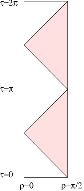
Figure 2: Horospheric coordinates only cover half of the whole anti de Sitter space ( namely the portion which is not filled).

In the AdS case however the solution of the related riemannian Laplace problem, that is, the operator obtained by replacing all minus signs by pluses in the metric, gives results for the propagator which are related by analytical continuation to the ones obtained with lorentzian signature (except for some subtleties related to the presence of normalizable modes ([23]).

This is not true anymore for the Goursat’s characteristic problem. Let us consider, the three-dimensional case to be specific. The analytical continuation of the hyperboloid

$$H_{\epsilon}\equiv t^{2}-x^{2}-y^{2}=\epsilon^{2}$$ (184)

is the sphere

$$S_{\epsilon}\equiv t^{2}+x^{2}+y^{2}=\epsilon^{2}$$ (185)

The solution to the exterior Dirichlet problem on the sphere $S_{\epsilon}$ for Laplace’s equation is given by the Poisson integral (cf. [10]) which expressed in three-dimensional polar coordinates reads

$$\Phi(R,\theta,\phi)=\frac{\epsilon(R^{2}-\epsilon^{2})}{4\pi}\int_{0}^{2\pi}d\phi^{\prime}\int_{0}^{\pi}d\theta^{\prime}\frac{f(\theta^{\prime},\phi^{\prime})sin\,\theta^{\prime}}{(\epsilon^{2}+R^{2}-2\epsilon Rcos\,\gamma)^{3/2}}$$ (186)

where $f(\theta,\phi)$ is the Dirichlet datum on $S_{\epsilon}$ and

$$cos\,\gamma\equiv cos\,\theta\,cos\,\theta^{\prime}sin\,\theta\,sin\,\theta^{\prime}\,cos\,(\phi-\phi^{\prime})$$ (187)

It will prove instructive to consider some examples in detail. In particular, the solution which reduces to

$$t^{2}\equiv\epsilon^{2}cos^{2}\,\theta$$ (188)

is easily found to be:

$$\Phi_{E}=\frac{\epsilon^{2}}{3}+\frac{2t^{2}-x^{2}-y^{2}}{3}$$ (190)

The corresponding analytic continuation

$$\Phi_{L}=\frac{\epsilon^{2}}{3}+\frac{2t^{2}+x^{2}+y^{2}}{3}$$ (191)

is indeed a solution of the wave equation with Lorentzian signature which reduces on $H_{\epsilon}$ to $t^{2}$. The problem is that from the point of view of $H_{\epsilon}$ $t^{2}$ and $r^{2}$ are the same thing, which is not true from the point of view of $S_{\epsilon}$.

For example, the solution of Laplace’s equation which reduces on $S_{\epsilon}$ to $r^{2}=x^{2}+y^{2}$ is

$$\Phi_{E}=\frac{2\epsilon^{2}}{3}+\frac{1}{3}(x^{2}+y^{2}-2t^{2})$$ (192)

which upon analytic continuation reduces to a solution which tends to $-\phi_{char}$ when $\epsilon\rightarrow 0$

In the same vein, one could consider the solution of Laplace’s equation which reduces to

$$\lambda t^{2}+(1-\lambda)(x^{2}+y^{2})$$ (193)

All of them are equivalent from the point of view of the characteristic problem. From the Laplace viewpoint, however, they are equivalent to $(1-\lambda)\epsilon^{2}+(2\lambda-1)t^{2}$. The result is

$$\Phi_{E}=\frac{(2-\lambda)\epsilon^{2}}{3}+\frac{2\lambda-1}{3}(2t^{2}-x^{2}-y^{2})=\frac{(2-\lambda)\epsilon^{2}}{3}+\frac{2\lambda-1}{3}R^{2}(2-3sin^{2}\,\theta).$$ (194)

(with $R^{2}\equiv t^{2}+x^{2}+y^{2}$), whose analytic continuation is

$$\Phi_{L}=\frac{(2-\lambda)\epsilon^{2}}{3}+\frac{2\lambda-1}{3}(2t^{2}+x^{2}+y^{2})$$ (195)

so that the characteristic solution is recovered when $\lambda=1$ only; the analytic continuation is inherently ambiguous.

Incidentally, we have been considering here up to now the interior solution of Laplace’s equation, whereas it would appear more appropiate to consider the exterior solution instead, which is easily obtained through an inversion

$$\Phi_{ext}(R,\theta,\phi)=\frac{\epsilon}{R}\phi_{int}(\frac{\epsilon^{2}}{R},\theta,\phi).$$ (196)

that is

$$\Phi_{ext}=\frac{(2-\lambda)\epsilon^{2}}{3}+\frac{2\lambda-1}{3}\frac{\epsilon^{5}}{R^{3}}(2-3sin^{2}\,\theta)$$ (197)

which does not have the correct analytic continuation.

Appendix D Goursat versus Cauchy

It is interesting to consider the Cauchy problem for initial data on the spacelike hypersurface $N_{\epsilon}(0)$

$$t^{2}-r^{2}=\epsilon^{2}=u.v$$ (198)

which degenerates into the cone $N_{+}(0)$ when $\epsilon\rightarrow 0$.

It could be thought that nothing changes much, but there is one essential point which does. Namely, the initial function is now

$$\psi(u)\equiv\phi(u,v=\frac{\epsilon^{2}}{u})$$ (199)

Deriving once and remembering that

$$f(u)\equiv\frac{\partial\phi}{\partial v}(u,v=\frac{\epsilon^{2}}{u})$$ (200)

yields in an obvious notation, evaluating all quantities at $N_{\epsilon}$

$$\partial_{u}\psi=\phi_{u}-\frac{\epsilon^{2}}{u^{2}}f$$ (201)

but there is now no restriction on the function f, given the fact that

$$f_{u}=\phi_{uv}-\frac{\epsilon^{2}}{u^{2}}\phi_{vv}$$ (202)

conveying that fact that now $\phi_{uv}$ is not uniquely determined in terms of (derivatives of) f.

We ask ourselves about the relation between the Cauchy and the characteristic problem for the wave equation of a scalar field $\phi$, the first posed on the hyperboloid $t^{2}-r^{2}=\epsilon^{2}$ with the value of the field and its normal derivative given, and the second on the future light cone $t=r$ with only the field known.

It seems that there is some preferred value for the field normal derivative such that in the limit $\epsilon\to 0$ the Cauchy problem goes to the characteristic one, that is, the derivative is somehow fixed and we only need the field itself.

In order to check these ideas, let work out one simple example in detail. We have a three dimensional solution to the wave equation with prescribed values on the surface $t^{2}-r^{2}=\epsilon^{2}$.

$$\phi=\frac{2t}{3}+\frac{\epsilon^{3}t}{3(t^{2}-r^{2})^{3/2}}$$ (203)

which obeys

$$\Box\phi=0$$

$$\left.\phi\right|_{t^{2}-r^{2}=\epsilon^{2}}=t$$

$$\left.\frac{d\phi}{dn}\right|_{t^{2}-r^{2}=\epsilon^{2}}=0$$ (204)

When $\epsilon\to 0$ the solution goes to

$$\hat{\phi}=\frac{2t}{3}$$ (205)

which is not the solution to the characteristic problem with the desired boundary value. But we also know this one, which is

$$\psi=t\qquad\to\qquad\psi|_{t^{2}-r^{2}=\epsilon^{2}}=t$$ (206)

The normal derivative of the Cauchy problem is $\frac{d}{dn}=\frac{1}{\epsilon}(t\partial_{t}+r\partial_{r})$ and it is not extended to the null surface. Nevertheless, taking the characteristic solution, we can perform the derivative $t\partial_{t}+r\partial_{r}$ and then regulate,

$$\frac{d}{dn}\phi=\frac{1}{\epsilon}(t\partial_{t}+r\partial_{r})\psi=\frac{t}{\epsilon}$$ (207)

We solve again the Cauchy problem with this prescribed derivative and find easily

$$\phi=\frac{2t}{3}+\frac{\epsilon^{3}t}{(t^{2}-r^{2})^{3/2}}+\frac{t}{3}\left(1-\frac{\epsilon^{3}}{(t^{2}-r^{2})^{3/2}}\right)$$ (208)

which satisfies

$$\Box\phi=0$$

$$\left.\phi\right|_{t^{2}-r^{2}=\epsilon^{2}}=t$$

$$\left.\frac{d\phi}{dn}\right|_{t^{2}-r^{2}=\epsilon^{2}}=\frac{t}{\epsilon}$$ (209)

This solution is precisely the desired one in the $\epsilon\to 0$ limit,

$$\phi|_{t^{2}-r^{2}=\epsilon^{2}}=\psi=t$$ (210)

Appendix E T-dual Formulation

It is possible to assume that the coordinates $y^{i}$ (cf. 2), $1\leq i\leq n$ live in an torus, for example

$$y^{i}=L\theta^{i}$$ (211)

This means that

$$x^{i}=\frac{L}{l}x_{-}\theta^{i}$$ (212)

That is, the combination $\frac{x^{i}}{x_{-}}$ must be a periodic function.

On the other hand, if

$$x^{i}=R\phi^{i}$$ (213)

then

$$y^{i}=\frac{lR}{x_{-}}\phi^{i}$$ (214)

Let us concentrate for example in this last possibility (213). The main difference with uncompactified Minkowski space is that now Goursat’s problem on the fundamental domain leads to a solution only in the diamond-like region highlighted in the figure. In order to get a solution on the whole space, data are needed on all lines

$$t=\pm r+nR$$ (215)

where $n\in\mathbb{N}$,

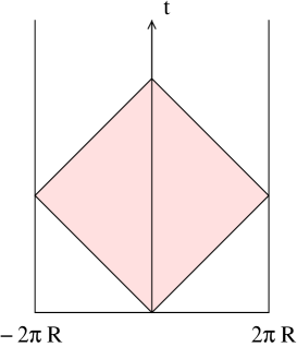
Figure 3: The fundamental diamond with angular coordinates.

If we interpret the full (n+2)-dimensional space as a string background (that is, we complete it with an extra internal Ricci-flat compact manifold of dimension $D=8-n$, and we interpret the scale $l$ as the string scale $l_{s}$) then it is known [14] to be equivalent to its T-dual.

This means, if for example (211) were true, that the gravitational background would read

$$d\tilde{s}^{2}=-\frac{l_{s}^{4}}{L^{2}T^{2}}d\vec{\tilde{\theta}}^{2}+\rho dT^{2}+TdTd\rho$$ (216)

with a nontrivial dilaton as well:

$$\Phi\equiv-\frac{n}{2}\log{\frac{T^{2}L^{2}}{l_{s}^{2}}}$$ (217)

This space is not flat, so that it cannot be equivalent to a wedge of Minkowski. Non-constant dilatons, however, are notoriously difficult to analyze.

References

- [1] E. Alvarez, J. Conde and L. Hernandez, “Codimension two holography,” Nucl. Phys. B 663 (2003) 365 [arXiv:hep-th/0301123].
- [2] E. Alvarez, “ The infinite curvature limit of AdS/CFT” [arXiv: gr-qc/0401097]
- [3] G. Arcioni and C. Dappiaggi, “Exploring the holographic principle in asymptotically flat spacetimes via Nucl. Phys. B 674 (2003) 553 [arXiv:hep-th/0306142].
- [4] S. J. Avis, C. J. Isham and D. Storey, “Quantum Field Theory In Anti-De Sitter Space-Time,” Phys. Rev. D 18 (1978) 3565.
- [5] T. Banks, W. Fischler, S. H. Shenker and L. Susskind, “M theory as a matrix model: A conjecture,” Phys. Rev. D 55 (1997) 5112 [arXiv:hep-th/9610043].
- [6] N. D. Birrell and P. C. Davies, “Quantum Fields In Curved Space,” (Cambridge University Press).
- [7] L. Blanchet, T. Damour and G. Esposito-Farese, “Dimensional regularization of the third post-Newtonian dynamics of point particles in harmonic coordinates,” arXiv:gr-qc/0311052.
- [8] J. D. Brown and J. W. . York, “Quasilocal energy and conserved charges derived from the gravitational action,” Phys. Rev. D 47 (1993) 1407.
- [9] J. D. Brown, S. R. Lau and J. W. . York, “Energy of Isolated Systems at Retarded Times as the Null Limit of Quasilocal Energy,” Phys. Rev. D 55 (1997) 1977 [arXiv:gr-qc/9609057].
- [10] R. Courant and D. Hilbert,Methods of Mathematical Physics, (Vol. 2) (Interscience, New York, 1962).
- [11] R. d’Adhemar,Sur une equation aux derivees partielles du type hyperbolique. Etude de l’integrale pres d’une frontiere characteristique. Palermo Rend. 20 (1905)142.
- [12] J. Erdmenger and H. Osborn, “Conserved currents and the energy-momentum tensor in conformally invariant Nucl. Phys. B 483 (1997) 431 [arXiv:hep-th/9605009].
- [13] C. Fefferman and C. Graham, Conformal Invariants Astérisque, hors série, 1985, p.95.
-
[14]
A. Giveon, M. Porrati and E. Rabinovici,
‘Target space duality in string theory,
Phys. Rept. 244 (1994) 77
[arXiv:hep-th/9401139].
E. Alvarez, L. Alvarez-Gaume and Y. Lozano, “An introduction to T duality in string theory,” Nucl. Phys. Proc. Suppl. 41 (1995) 1 [arXiv:hep-th/9410237]. - [15] J. Hadamard,Lectures on the Cauchy problem in linear partial differential equations. (Dover, New York, 1952).
- [16] Fritz John, Plane waves and spherical means, (Springer, New York, 1955).
- [17] C. C. Liu and S. T. Yau, “New definition of quasilocal mass and its positivity,” arXiv:gr-qc/0303019.
- [18] J. Maldacena, The large N limit of superconformal field theories and supergravity, Adv.Theor.Math.Phys.2:231-252,1998, hep-th/9711200.
- [19] R. Penrose and W. Rindler, “Spinors And Space-Time. 1. Two Spinor Calculus And Relativistic Fields,” (Cambridge, 1984).
- [20] Marcel Riesz, L’integrale de Riemann-Liouville et le probleme de Cauchy. Acta Mathematica, 81 (1949),1.
- [21] L. Susskind, “The World as a hologram,” J. Math. Phys. 36 (1995) 6377 [arXiv:hep-th/9409089].
- [22] G. ’t Hooft, “Dimensional Reduction In Quantum Gravity,” arXiv:gr-qc/9310026.
-
[23]
E. Witten,
“Anti-de Sitter space and holography,”
Adv. Theor. Math. Phys. 2 (1998) 253
[arXiv:hep-th/9802150].
E. Witten, “Anti-de Sitter space, thermal phase transition, and confinement in gauge theories,” Adv. Theor. Math. Phys. 2 (1998) 505 [arXiv:hep-th/9803131]. - [24] E. Witten, talk in Strings 98, on line at http://online.itp.ucsb.edu/online/strings98/witten