The entropy of black holes: a primer

Abstract

After recalling the definition of black holes, and reviewing their energetics and their classical thermodynamics, one expounds the conjecture of Bekenstein, attributing an entropy to black holes, and the calculation by Hawking of the semi-classical radiation spectrum of a black hole, involving a thermal (Planckian) factor. One then discusses the attempts to interpret the black-hole entropy as the logarithm of the number of quantum micro-states of a macroscopic black hole, with particular emphasis on results obtained within string theory. After mentioning the (technically cleaner, but conceptually more intricate) case of supersymmetric (BPS) black holes and the corresponding counting of the degeneracy of Dirichlet-brane systems, one discusses in some detail the “correspondence” between massive string states and non-supersymmetric Schwarzschild black holes.

I Black holes

Let us start by briefly reviewing the concept of black hole. Within a couple of months after Einstein’s discovery of the final form of the field equations of General Relativity, Karl Schwarzschild succeeded in writing down the exact form of the general relativistic analog of the “gravitational field of a mass point” [1], namely (in the coordinates introduced by Johannes Droste) the general spherically-symmetric solution of Einstein’s vacuum field equations $(R_{\mu\nu}=0)$:

$$ds_{\rm SCHW}^{2}=g_{\mu\nu}^{\rm SCHW}(x^{\lambda})\,dx^{\mu}\,dx^{\nu}=-\left(1-\frac{2GM}{c^{2}r}\right)c^{2}\,dt^{2}+\frac{dr^{2}}{1-\frac{2GM}{c^{2}r}}+r^{2}(d\theta^{2}+\sin^{2}\,\theta\,d\varphi^{2})\,.$$ (1)

Here, $G$ denotes Newton’s constant and $M$ denotes the (total) mass of the considered object, as it can be measured from infinity (e.g. by comparing the motion of far-away test particles in the metric (1) to that of test particles in the Newtonian potential $U({\mathbf{x}})=GM/r$).

It was soon noticed that the metric (1) has an apparently singular behaviour at the “Schwarzschild radius” $r_{S}\equiv 2GM/c^{2}$. For instance, a clock at rest in the metric (1) and located at a radius $r$ ($r>r_{S}$) exhibits, when its ticks are “read” from infinity via electromagnetic signals, a redshift equal to

$$\frac{[ds]^{\text{read at}}_{\text{infinity}}}{[ds]^{\text{measured}}_{\text{locally}}}=\frac{\sqrt{-g_{00}(r=\infty)}}{\sqrt{-g_{00}(r)}}=\frac{1}{\sqrt{1-\frac{2GM}{c^{2}r}}}\,.$$ (2)

The redshift (2) goes to infinity as $r\to r_{S}$ . Therefore the “Schwarzschild sphere” $r=r_{S}=2GM/c^{2}$ has the observable characteristic of being an infinite-redshift surface. Similarly, one finds that the force needed to keep a particle at rest at a radius $r>r_{S}$ goes to infinity as $r\to r_{S}$.

It took many years, and the work of many scientists (notably Oppenheimer and Snyder, Kruskal and Penrose), to decipher the physical meaning of these infinities occurring at the “Schwarzschild sphere”. This understanding is summarized in the spacetime diagram of Fig. 1.

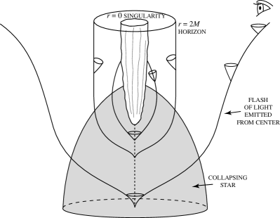
FIG. 1.: Spacetime representation of the formation of a black hole by the collapse of a star. The horizon is the spacetime history of a bubble of light (i.e. a null hypersurface) which stabilizes itself under the strong pull of relativistic gravity

The 2-dimensional surface $r=r_{S}$, becomes, when adding the time dimension, a 3-dimensional hypersurface ${\mathcal{H}}$ in spacetime. The hypersurface ${\mathcal{H}}$ is a fully regular submanifold of a locally regular spacetime. To see the regularity of ${\mathcal{H}}$, one needs to change coordinates near $r=r_{S}$. For instance, one can use the ingoing Eddington-Finkelstein coordinates $(v,r,\theta,\varphi)$, where $v=t+r_{*}$, with $r_{*}$ defined as

$$r_{*}=\int\frac{dr}{1-\frac{2GM}{c^{2}r}}=r+\frac{2GM}{c^{2}}\ln\left(\frac{c^{2}r}{2GM}-1\right)\,.$$ (3)

In these coordinates the Schwarzschild metric reads

$$ds_{\rm SCHW}^{2}=-\left(1-\frac{2GM}{c^{2}r}\right)\,dv^{2}+2dvdr+r^{2}(d\theta^{2}+\sin^{2}\,\theta\,d\varphi^{2})\,.$$ (4)

In these coordinates the horizon is located at $r=r_{S}$, the other coordinates $(v,\theta,\varphi)$ taking arbitrary, but finite values. [Note that a finite value of the new “time variable” $v$ corresponds to an infinite (and positive) value of the original Schwarzschild time coordinate $t$.] One easily checks that the geometry ( 4) is regular near $r=r_{S}$.

One can then see that the hypersurface ${\mathcal{H}}$ ($r=r_{S}$) is a quite special submanifold in that it is a null hypersurface, i.e. a co-dimension-1 surface which is locally tangent to the light cone. In other words, the (co-)vector normal to the hypersurface, say $\ell_{\mu}$ (such that $\ell_{\mu}\,dx^{\mu}=0$ for all directions $dx^{\mu}$ tangent to the hypersurface) is a null vector: $0=g^{\mu\nu}\ell_{\mu}\,\ell_{\nu}=g_{\mu\nu}\,\ell^{\mu}\ell^{\nu}$. As a consequence $\ell^{\mu}$ is both normal and tangent to the hypersurface (because $\ell_{\mu}\,\ell^{\mu}=0$). The local light cone, $g_{\mu\nu}(x)\,dx^{\mu}\,dx^{\nu}=0$, is tangent to ${\mathcal{H}}$ along the special direction $\ell^{\mu}$. [This gives a special, fibered structure to ${\mathcal{H}}$, generated by the lines tangent to $\ell^{\mu}$, called the “generators” of ${\mathcal{H}}$.] Physically, the tangency between ${\mathcal{H}}$ and the local light cone (and the fact that the spatial sections of ${\mathcal{H}}$ are compact) means that ${\mathcal{H}}$ is the boundary between the part of spacetime from which light can escape to infinity, and the part out of which light cannot so escape. This boundary is called the (future) Horizon (hence the notation ${\mathcal{H}}$).

Fig. 1 illustrates the fact that the Horizon ${\mathcal{H}}$ is a dynamical, time-evolving structure. In the simple, spherically-symmetric situation assumed in Fig. 1, the horizon ${\mathcal{H}}$ is the spacetime history of a special bubble of light that was emitted from the center of a collapsing star, and which, after expanding out from the center, stabilized itself, under the strong pull of relativistic gravity, into an asymptotically stationary configuration, which is precisely the (time-independent) Schwarzschild sphere $r=r_{S}\equiv 2GM/c^{2}$. The structure illustrated by Fig. 1 is called a black hole. The “interior” of ${\mathcal{H}}$ is the interior of the black hole (spacetime region where light is “trapped”, i.e. cannot escape to infinity), while ${\mathcal{H}}$ (which marks the great “divide” between trapped light, and light escaping at infinity) is the horizon, or the surface of the black hole. Note the presence, inside the black hole, of an infinite spacetime volume which ends, in its future, in a spacelike singularity at $r=0$ (where the curvature blows up as $r^{-3}$). This singularity is a “big crunch” singularity: it is of a cosmological type (the coordinate $r$ of Eq. (1) being “time-like” when $r<r_{S}$), and a time-reverse analog of the familiar Friedmann big-bang singularity.

A lot of work (for references, see, e.g., [2, 3, 4, 5, 6]) went into understanding how general is the picture of Fig. 1. The stability (near and outside ${\mathcal{H}}$) of the spherical collapse situation of Fig. 1 under small, non-spherically-symmetric perturbations, the existence of multi-parameter generalizations of the Schwarzschild metric (due to Reissner, Nordstrøm, Kerr, Newman et al.) featuring regular horizon structures, and the proof of several “no-hair” theorems (by Israel, Carter, etc.), led to the following (conjectural) picture. The gravitational collapse of any type of matter configuration will generically lead to the formation of a black hole, whose surface is a null hypersurface ${\mathcal{H}}$, and will asymptotically settle into a stationary state, which is completely described (if the black hole is isolated) by a small number of parameters. When considering, as long range fields, only gravity $(g_{\mu\nu})$ and electromagnetism $(A_{\mu})$, the final, stationary configuration of a black hole is described by three parameters, its total mass $M$, its total angular momentum $J$, and its total electric charge $Q$, and is given by the following Kerr-Newman solution

$$ds_{\rm KN}^{2} = -\frac{\Delta}{\Sigma}\,\omega_{t}^{2}+\frac{\Sigma}{\Delta}\,dr^{2}+\Sigma d\theta^{2}+\frac{\sin^{2}\theta}{\Sigma}\,\omega_{\varphi}^{2}\,,$$ (6)

$$A_{\mu}^{\rm KN}\,dx^{\mu} = -\frac{Qr}{\Sigma}\omega_{t}\,,$$ (7)

$$\frac{1}{2}\,F_{\mu\nu}^{\rm KN}\,dx^{\mu}\wedge dx^{\nu} = \frac{Q}{\Sigma^{2}}\,(r^{2}-a^{2}\cos^{2}\theta)\,dr\wedge\omega_{t}+\frac{2Q}{\Sigma^{2}}\,ar\cos\theta\sin\theta\,d\theta\wedge\omega_{\varphi}\,,$$ (8)

where (setting for simplicity $G=c=1$)

$$a\equiv\frac{J}{M}\,,\quad\Delta=r^{2}-2Mr+a^{2}+Q^{2}\,,\quad\Sigma=r^{2}+a^{2}\cos^{2}\theta\,,$$

$$\omega_{t}=dt-a\sin^{2}\theta\,d\varphi\,,\quad\omega_{\varphi}=(r^{2}+a^{2})\,d\varphi-a\,dt\,.$$ (9)

The Kerr-Newman field configuration (1) is a black hole (with a regular horizon ${\mathcal{H}}$) if and only if the three parameters $M$, $J$, $Q$ satisfy the inequality (recall the notation $a\equiv J/M$, and the choice of units $c=G=1$ that will often be used below)

$$a^{2}+Q^{2}\leq M^{2}\,.$$ (10)

The black holes that saturate the inequality (10), i.e. those that satisfy $a^{2}+Q^{2}=M^{2}$, are called extremal. Note that a Schwarzschild black hole ($a=Q=0$) can never be extremal, while a Reissner-Nordstrøm black hole ($a=0$) is extremal when $|Q|=M$ (i.e. $|Q|=G^{\frac{1}{2}}M$), and a Kerr black hole ($Q=0$) is extremal when $|a|=M$ (i.e. $J=GM^{2}$). By analyzing the spacetime geometry (6) one finds that the horizon of a Kerr-Newman black hole is located (when viewed at “constant time”) on the surface $r=r_{+}$ with

$$r_{+}\equiv M+\sqrt{M^{2}-a^{2}-Q^{2}}\,.$$ (11)

II Energetics and thermodynamics of black holes

It is very fruitful to consider a black hole as a kind of gravitational soliton, i.e. as a physical object, localized “within the horizon ${\mathcal{H}}$”, generating the “external fields” (1), and possessing a total mass $M$, a total angular momentum $J$ and a total electric charge $Q$. By dropping massive, charged test particles, moving on generic non radial orbits, one then expects that it is possible to change the values of $M$, $J$ and $Q$, i.e. to evolve from an initial Kerr-Newman black hole state $(M,J,Q)$ to a final one ($M+\delta M$, $J+\delta J$, $Q+\delta Q$) where $\delta M=E$, $\delta J=p_{\varphi}$ and $\delta Q=e$. Here $E=-p_{t}=-\partial S/\partial t$ is the conserved energy of the test particle freely moving (geodesic motion) in the background Kerr-Newman configuration $(M,J,Q)$, $p_{\varphi}=\partial S/\partial\varphi$ its conserved ($z$-component of the) angular momentum, and $e$ its electric charge. [$S$ denotes here the action of the test particle, satisfying the Hamilton-Jacobi equation $g^{\mu\nu}(p_{\mu}-eA_{\mu})(p_{\nu}-eA_{\mu})=-\mu^{2}$, where $p_{\mu}=\partial S/\partial x^{\mu}$ is its 4-momentum and $\mu$ its mass.] It was first realized by Penrose [7] that such a process can lead, in certain (special) circumstances, to a decrease of the total mass of the black hole: $\delta M<0$. A detailed analysis of the changes of $M$, $J$ and $Q$ during the absorption of test particles, then led Christodoulou [8] and Christodoulou and Ruffini [9] to introduce the concepts of reversible transformation and of irreversible transformation of a black hole. More precisely, starting from $\delta M=-p_{t}$, $\delta J=p_{\varphi}$, $\delta Q=e$ and from the mass-shell constraint $g^{\mu\nu}(p_{\mu}-eA_{\mu})(p_{\nu}-eA_{\nu})=-\mu^{2}$ (which gives a quadratic equation to determine the energy $-p_{t}$ in terms of $p_{\varphi}$, $e$ and the other components of $p_{\mu}$, namely $p_{r}$ and $p_{\theta}$), they derived, when considering a particle crossing the horizon, i.e. being absorbed by the black hole, the following equality

$$\delta M-\frac{a\,\delta J+r_{+}\,Q\,\delta Q}{r_{+}^{2}+a^{2}}=\frac{r_{+}^{2}+a^{2}\cos^{2}\theta}{r_{+}^{2}+a^{2}}|p^{r}|\,,$$ (12)

the right-hand side of which is proportional to the absolute value of the radial momentum of the particle as it enters the black hole. [The latter absolute value comes from taking a positive square root, similarly to the usual special relativistic result $E=+\sqrt{{\mu}^{2}+{\bf p}^{2}}$.] The positivity of the latter quantity then leads to deriving the inequality

$$\delta M\geq\frac{a\,\delta J+r_{+}\,Q\,\delta Q}{r_{+}^{2}+a^{2}}\,.$$ (13)

A reversible transformation is then defined as a transformation which saturates the inequality (13), i.e. where one replaces $\geq$ by an equality sign. It is called “reversible” because, after having (algebraically) added $\delta J$ and $\delta Q$ (and the corresponding $\delta M=$ R.H.S. of (13)) to a black hole, the subsequent reversible “addition” of $\delta^{\prime}J=-\delta J$, $\delta^{\prime}Q=-\delta Q$ (and the corresponding, saturated $\delta^{\prime}M=-\delta M$) will lead to a final state $(M+\delta M+\delta^{\prime}M,J+\delta J+\delta^{\prime}J,Q+\delta Q+\delta^{\prime}Q)\equiv(M,J,Q)$, i.e. identical to the initial state. By contrast, a sequence of infinitesimal transformations where at least one of the elementary processes (13) contains the strict inequality sign $>$ cannot be reversed.

By integrating the differential equation obtained by saturating (13) one obtains the Christodoulou-Ruffini mass formula of black holes,

$$M^{2}=\left(M_{\rm irr}+\frac{Q^{2}}{4M_{\rm irr}}\right)^{2}+\frac{J^{2}}{4M_{\rm irr}^{2}}\,,$$ (14)

where the irreducible mass $M_{\rm irr}$ is an (integration) constant under reversible processes, and varies in the following irreversible manner,

$$\delta M_{\rm irr}\geq 0\,,$$ (15)

under general, possibly irreversible, processes. One also finds that the irreducible mass can be explicitly (rather than implicitly as in Eq. (14)) expressed in terms of $M$, $J$ and $Q$ as

$$M_{\rm irr}=\frac{1}{2}\,\sqrt{r_{+}^{2}+a^{2}}\,.$$ (16)

Note that Eq. (14) says that the “free energy” of a black hole, i.e. the maximal energy which can be extracted by depleting (in a reversible) way $J$ and $Q$ is $M-M_{\rm irr}$. This free energy has both Coulomb $(\propto Q^{2})$ and rotational $(\propto J^{2})$ contributions. It vanishes in the case of a Schwarzschild black hole ($J=0=Q$).

For our present purpose, a crucial aspect of the global energetics of black holes, given by Eq. (14), is the striking similarity of the irreversible increase (15) of the irreducible mass with the second law of thermodynamics, i.e. the irreversible increase of the total entropy $S$ of an isolated system. A general theorem of Hawking [10] led to a deeper understanding of the irreversible behaviour (15). Indeed, starting from the basic geometrical fact that a horizon is a null hypersurface, and analyzing the global properties of the generators of the horizon, Hawking proved that the area $A$ of successive time sections of the horizon of a black hole cannot decrease,

$$\delta A\geq 0\,.$$ (17)

He also proved that, if one considers a system made of several, separate black holes, the sum of the areas of all the horizons cannot decrease

$$\delta\left(\sum_{a}A_{a}\right)\geq 0\,.$$ (18)

In the particular case of a Kerr-Newman hole the result (17) yields back (15). Indeed, one easily finds from Eq. (6), when using $r=r_{+}$ (i.e. $\Delta=0$ and $dr=0$) that the inner geometry of the horizon is $d\sigma^{2}=\gamma_{AB}(x^{C})\,dx^{A}\,dx^{B}=(r_{+}^{2}+a^{2}\cos^{2}\theta)\,d\theta^{2}+\sin^{2}\theta(r_{+}^{2}+a^{2})^{2}\,d\varphi^{2}/(r_{+}^{2}+a^{2}\cos^{2}\theta)$ (with $A,B=1,2=\theta,\varphi$ in the example at hand), so that the area of (a time section) of the horizon is

$$A_{\rm KN}=\int\int(r_{+}^{2}+a^{2})\sin\theta\,d\theta\,d\varphi=4\pi(r_{+}^{2}+a^{2})=16\pi M_{\rm irr}^{2}\,.$$ (19)

In view of Eqs. (15), (17), (18) it is tempting to attribute to a black hole, considered as a physical object, not only a total mass $M$, a total angular momentum, and a total electric charge, but also a total entropy, proportional to the area of the horizon, say

$$S_{\rm BH}=\alpha A\,,$$ (20)

where $\alpha$ is a constant with dimension of inverse length squared. By varying the mass formula (14) one then finds the “first law of the thermodynamics of black holes”,

$$dM=\Omega\,dJ+\Phi\,dQ+T_{\rm BH}\,dS_{\rm BH}\,,$$ (21)

where (see Eq. (13)) $\Omega=a/(r_{+}^{2}+a^{2})$ can be interpreted as the angular velocity of the black hole, $\Phi=Q\,r_{+}/(r_{+}^{2}+a^{2})$ as its electric potential (see [2] for discussions of $\Omega$ and $\Phi$), and where

$$T_{\rm BH}\equiv\frac{1}{\alpha}\frac{\partial M}{\partial A}=\frac{\kappa}{8\pi\alpha}$$ (22)

is expected to represent the “temperature” of the black hole. The quantity $\kappa$ in Eq. (22) is the surface gravity of a black hole, generally defined as the coefficient relating the covariant directional derivative of the horizon normal vector $\ell^{\mu}$ along itself to $\ell^{\mu}:\ell^{\nu}\,\nabla_{\nu}\,\ell^{\mu}=\kappa\,\ell^{\mu}$. [Here, $\ell^{\mu}$ is normalized so that, on the horizon, $\ell^{\mu}\,\partial_{\mu}=\partial_{t}+\Omega\,\partial_{\varphi}$ where $\partial_{t}$ is the usual Killing vector of time translations.] The surface gravity may be thought of as the redshifted acceleration of a particle staying “still” on the horizon. [As we said above, the proper-time acceleration of a particle sitting on the horizon is actually infinite, but the infinite redshift factor associated to the difference between the proper time and the “time” associated to the generator $\ell^{\mu}$ compensates for this infinity.]

In the case of a Kerr-Newman hole, the value of the surface gravity reads $(r_{\pm}\equiv M\pm\sqrt{M^{2}-a^{2}-Q^{2}})$

$$\kappa=\frac{1}{2}\,\frac{r_{+}-r_{-}}{r_{+}^{2}+a^{2}}=\frac{\sqrt{M^{2}-a^{2}-Q^{2}}}{r_{+}^{2}+a^{2}}\,.$$ (23)

Note that the surface gravity of a Schwarzschild black hole is given by the usual formula for the surface gravity of a massive star, i.e. $\kappa=GM/r_{S}^{2}=M/(2M)^{2}=1/(4M)$. Note also that the surface gravity (and therefore the expected “temperature”) of extremal black holes vanishes.

The “first law of black-hole thermodynamics” (21) has been derived above in the particular (but particularly important!) case of Kerr-Newman black holes. A general derivation, for generic (non isolated) black-hole equilibrium states, has been given by Carter [11] and by Bardeen, Carter and Hawking [12]. For a recent review of black-hole thermodynamics, see [13]. See also these references for a discussion of the “zeroth law of black-hole thermodynamics”, namely the constancy of the “temperature” (22), i.e. of the surface gravity $\kappa$, all over the horizon. [In the “membrane” approach to black-hole physics [16], the uniformity of $\kappa$ for stationary states is viewed as a consequence of the Navier-Stokes equation because the “surface pressure” of a black hole happens to be equal to $p\equiv\kappa/8\pi$.]

Before going on to considering quantum aspects of the irreversibility of black hole evolution, let us complete our brief description of the classical dynamics and thermodynamics of black holes by mentioning that the irreversibility (15) or (17) affecting a global characteristic of a black hole has its roots in the irreversible behaviour of a local characteristic of the horizon. It proved fruitful to view a black hole as a kind of membrane [14, 15, 16], fibered by the generators (see above), and endowed with familiar physical properties: pressure $p=\kappa/8\pi$, shear viscosity $\eta$, bulk viscosity $\zeta$, resistivity $\rho$. For instance, one can write an Ohm’s law relating the electromotive force tangent to the horizon to the current flowing in the horizon, and a Navier-Stokes equation relating the time-evolution of the black-hole surface momentum density to the (surface) gradient of the pressure, to the effects of the shear and of the expansion of the “2-dimensional” fluid of generators and to a possible external flux of momentum. Starting from Einstein’s equations one finds, e.g., that the (surface) resistivity of black holes is $\rho=377$ ohm (i.e. $4\pi$), and that their (surface) shear viscosity is $\eta=(16\pi)^{-1}$. Of particular interest for our present purpose is the existence of a local (i.e. at each point of the surface of the black hole) version of the “second law of thermodynamics”. Let us “localize” the global attribution (20) by attributing an entropy

$$dS_{\rm BH}=\alpha\,dA$$ (24)

to each area element $dA$ of the horizon. This local entropy is then found to evolve, as a consequence of Einstein’s equations, in the following irreversible manner [17, 16]

$$\frac{d}{dt}\,(dS_{\rm BH})-\tau\,\frac{d^{2}}{dt^{2}}\,(dS_{\rm BH})=\frac{dA}{T_{\rm BH}}\left[2\eta\,\sigma_{\rm AB}\,\sigma^{\rm AB}+\zeta\,\theta^{2}+\rho\,({\mathbf{J}}_{\rm BH}-\sigma_{\rm BH}\,{\mathbf{v}})^{2}\right]\,.$$ (25)

Here, $d/dt$ is a convective derivative (along the generators), $\tau\equiv\kappa^{-1}$ a characteristic time scale, $\eta$ the shear viscosity mentioned above, $\sigma_{\rm AB}$ the shear tensor of the 2-dimensional fluid motion, $\zeta=-\eta$ the bulk viscosity, $\theta$ the local rate of dilatation of the fluid motion, $\rho$ the (surface) resistivity, ${\mathbf{J}}_{\rm BH}-\sigma_{\rm BH}{\mathbf{v}}$ the horizon’s conduction current (total current ${\mathbf{J}}_{\rm BH}$ minus convection current $\sigma_{\rm BH}{\mathbf{v}}$, where $\sigma_{\rm BH}$ is the horizon’s surface charge density), and where $T_{\rm BH}$ can be interpreted as the local temperature of the horizon

$$T_{\rm BH}\equiv\frac{\kappa}{8\pi\alpha}\,,$$ (26)

where $\kappa$ (defined as above by $\ell^{\nu}\,\nabla_{\nu}\,\ell^{\mu}\equiv\kappa\,\ell^{\mu}$) is the local value of the surface gravity. [The surface gravity is uniform, on the horizon, for stationary black holes, but is generically non-uniform for evolving black holes.]

In the limit of an adiabatically slow evolution of the black-hole state, Eq. (25) reduces to the usual thermodynamical law giving the local increase of the entropy of a fluid element heated by the dissipations associated to viscosity and the Joule’s law. [For non adiabatic evolutions, the L.H.S. of Eq. (25) can be interpreted, similarly to the famous a-causal Lorentz-Dirac radiation-reaction equation, in terms of an anticipated response of the black hole to external sollicitations [18, 16].]

III Bekenstein’s entropy and Hawking’s temperature

The striking similarity between the irreversible increase of the area of the horizon of a black hole, reviewed in the last Section, and the second law of thermodynamics, motivated Bekenstein [19, 20, 21] to introduce the concept of black-hole entropy, say $S_{\rm BH}$. [See the Appendix for John Wheeler’s account [22] of how Jacob Bekenstein started to think about the concept of black-hole entropy and see Bekenstein’s own account in [23].] He gave several arguments suggesting that $S_{\rm BH}$ is (as anticipated in the previous Section) proportional to the area $A$ of the black hole, and of the form

$$S_{\rm BH}=\hat{\alpha}\,\frac{c^{3}}{\hbar G}\,A\equiv\hat{\alpha}\,\frac{A}{\ell_{P}^{2}}\,,$$ (27)

where $\hat{\alpha}$ is a universal dimensionless number of order unity, and where $\ell_{P}\equiv\sqrt{\hbar G/c^{3}}$ denotes the Planck length. [We set Boltzmann’s constant to unity.]

One of the arguments used by Bekenstein was an analysis of the quantum limitations on the existence of reversible transformations, in the sense of Christodoulou [8]. Indeed, from Eq. (12) above the inequality (13) can be saturated only in the limit where the particle captured by the black hole has exactly zero radial momentum on the horizon. He considered that, in order of magnitude, quantum effects impose a minimal (proper) size, for a particle of mass $\mu$, of order its Compton wavelength $\lambda_{c}=\hbar/\mu c$, so that a particle can never be located exactly on the horizon, but only within an uncertainty $\sim\lambda_{c}$ in proper distance. Bekenstein then found that this uncertainty implied the existence of a lower bound on the difference between the L.H.S. and the R.H.S. of Eq. (13). When estimating the corresponding lower bound on the increase of the area of a black hole as it captures a particle, he found a value of order $\hbar G/c^{3}=\ell_{P}^{2}$, seemingly independent of all the characteristics of both the black hole and the particle.

Considering that, as a particle goes down a black hole, one looses (because of the no-hair theorems) an information of the order of one bit, and following Brillouin in identifying information with negative entropy [24], he estimated that the dimensionless constant $\hat{\alpha}$ in Eq. (27) was probably numerically $\simeq(\ln 2)/(8\pi)$. In other words, Bekenstein’s black-hole entropy was viewed by him as a measure of the information about the interior of a black hole which is inaccessible to an external observer. He gave several other arguments leading to a result of the form (27), including an argument based on the analysis of quantum limitations on the efficiency of Carnot cycles using a black hole as heat sink. The latter argument suggested the need to attribute to a black hole a temperature of order of that corresponding (in the sense of Eqs. (20)–(22) above, with $\alpha\equiv\hat{\alpha}\,c^{3}/(\hbar G)$) to the entropy (27), i.e.

$$T_{\rm BH}=\frac{1}{8\pi\hat{\alpha}}\,\frac{\hbar}{c}\,\kappa\,,$$ (28)

where $\kappa$ denotes the surface gravity of the black hole. [A factor $G/c^{2}$ disappeared between (27) and (28) because we measure here $\kappa$ in the usual way surface gravities are measured: $\kappa\sim GM/r^{2}=c^{2}/{\rm length}$.] Finally, Bekenstein conjectured the validity of a generalized version of the second law of thermodynamics, stating that the sum of the black-hole entropy (27) and of the ordinary entropy in the exterior of the black hole never decreases.

Bekenstein’s arguments could not yield a precise determination of the dimensionless coefficient $\hat{\alpha}$ in Eq. (27) or (28) (nor could they really establish the universality of this coefficient). Soon after Bekenstein’s original suggestions, Hawking (who, initially, did not believe that it made sense to attribute a non-zero temperature (28) to a black hole) discovered the universal phenomenon of quantum radiance of black holes [25, 26]. This work gave a precise meaning to a black-hole temperature of the form (28). More precisely, Hawking found

$$T_{\rm BH}=\frac{1}{2\pi}\,\frac{\hbar}{c}\,\kappa\,,$$ (29)

which exactly corresponds to Eq. (28) if (and only if) the dimensionless coefficient $\hat{\alpha}$ there is equal to

$$\hat{\alpha}=\frac{1}{4}\,.$$ (30)

In view of the importance of Hawking’s result [25, 26], let us (following [27]) give a simplified derivation of the phenomenon of quantum radiance. Let us consider (for simplicity) a massless scalar field $\varphi(x)$ propagating in a Schwarzschild background. The quantum excitations of $\varphi(x)$ can be decomposed into classical mode functions, say

$$\varphi_{\omega\ell m}(t,r,\theta,\varphi)=\frac{e^{-i\omega t}}{\sqrt{2\pi|\omega|}}\,\frac{u_{\omega\ell m}(r)}{r}\,Y_{\ell m}(\theta,\varphi)\,,$$ (31)

which must satisfy

$$0=\Box_{g}\,\varphi=\frac{1}{\sqrt{g}}\,\partial_{\mu}(\sqrt{g}\,g^{\mu\nu}\,\partial_{\nu}\,\varphi)\,.$$ (32)

Before tackling the application of Eq. (32) to a Schwarzschild background, let us recall the essentials of the theory of particle creation by a background field. The quantum operator $\hat{\varphi}(x)$ describing (real, massless) scalar particles can be decomposed both with respect to some “in” basis of modes (describing free, incoming particles), say

$$\hat{\varphi}(x)=\sum_{i}\hat{a}_{i}^{\rm in}\,p_{i}^{\rm in}(x)+(\hat{a}_{i}^{\rm in})^{+}\,n_{i}^{\rm in}(x)\,,$$ (33)

and with respect to an “out” basis of modes (describing outgoing particles), say

$$\hat{\varphi}(x)=\sum_{i}\hat{a}_{i}^{\rm out}\,p_{i}^{\rm out}(x)+(\hat{a}_{i}^{\rm out})^{+}\,n_{i}^{\rm out}(x)\,.$$ (34)

Here the $\hat{a}^{\rm in}$, $(\hat{a}^{\rm in})^{+}$, $\hat{a}^{\rm out}$, $(\hat{a}^{\rm out})^{+}$ are two sets of annihilation and creation operators (with, e.g., $[\hat{a}_{i}^{\rm in},(\hat{a}_{j}^{\rm in})^{+}]=\delta_{ij}$) corresponding to a decomposition in modes which can physically be considered as incoming positive-frequency ones $(p_{i}^{\rm in}(x))$, incoming negative-frequency ones ($n_{i}^{\rm in}(x)$; which can be taken to be the complex conjugate of $p_{i}^{\rm in}(x)$ in our case), outgoing positive-frequency ones $(p_{i}^{\rm out}(x))$ and outgoing negative-frequency ones $(n_{i}^{\rm out}(x))$. These mode functions are normalized so that, say, $(p_{i}^{\rm in},p_{j}^{\rm in})=\delta_{ij}$, $(p_{i}^{\rm in},n_{j}^{\rm in})=0$, $(n_{i}^{\rm in},n_{j}^{\rm in})=-\delta_{ij}$, where $(\varphi_{1},\varphi_{2})$ denotes the standard (conserved) Klein-Gordon scalar product.

The “in” vacuum is defined by $\hat{a}_{i}^{\rm in}|{\rm in}\rangle=0$, and the mean number of $i$-type “out” particles present in the in-vacuum is given by

$$\langle N_{i}\rangle=\langle{\rm in}|\,(a_{i}^{\rm out})^{+}\,a_{i}^{\rm out}\,|{\rm in}\rangle=\sum_{j}|T_{ij}|^{2}$$ (35)

where $T_{ij}\equiv(p_{i}^{\rm out},n_{j}^{\rm in})$ is the (standard Klein-Gordon) scalar product, i.e. physically the transition amplitude, between the incoming negative-frequency mode $n_{j}^{\rm in}$ and the outgoing positive-frequency one $p_{i}^{\rm out}$. In the black-hole case the in-vacuum will be defined by focussing on high-frequency wave packets propagating in the vicinity of the horizon ${\mathcal{H}}$, say some $n_{j}^{\rm in}(x)$, and frequency-analyzed in a local freely-falling frame. We will then be interested in the transition amplitude between such an incoming $n_{j}^{\rm in}(x)$ and an outgoing mode which reaches (future) infinity as a positive-frequency wave-packet (in the usual sense of the decomposition (31) there).

Inserting the explicit form (1) of the Schwarzschild metric into Eq. (32), using the mode decomposition (31), and introducing the usual “tortoise” radial coordinate [4]

$$r_{*}=\int\frac{dr}{1-\frac{2M}{r}}=r+2M\ln\left(\frac{r-2M}{2M}\right)\,,$$ (36)

leads to the following radial equation for $u_{\omega\ell m}(r)$:

$$\frac{\partial^{2}u}{\partial r_{*}^{2}}+(\omega^{2}-V_{\ell}\,[r(r_{*})])\,u=0\,,$$ (37)

where the effective radial potential $V_{\ell}$ reads

$$V_{\ell}(r)=\left(1-\frac{2M}{r}\right)\left(\frac{\ell(\ell+1)}{r^{2}}+\frac{2M}{r^{3}}\right)\,.$$ (38)

In the coordinate $r_{*}$, the horizon ($r=2M$) is located at $r_{*}\to-\infty$, i.e. in the left asymptotic region of the potential $V_{\ell}\,[r(r_{*})]$, where $V_{\ell}$ tends exponentially towards zero. [Note that $V_{\ell}\,[r(r_{*})]$ tends to zero both as $r_{*}\to-\infty$ ($r\to 2M$) and as $r_{*}\to+\infty$ ($r\to+\infty$), and creates a positive potential barrier around $r\sim 3M$.] Neglecting the potential $V_{\ell}$ in Eq. (37), we see that, near the horizon, the radial function $u(r_{*})$ behaves as $e^{\pm i\omega r_{*}}$, so that (after factoring $1/r$ and $Y_{\ell m}(\theta,\varphi)$) the mode function (31) behaves there as

$$\varphi_{\omega}(t,r)\propto e^{-i\omega(t\pm r_{*})}\,.$$ (39)

At this point we need to recall that the “singularity” of the Schwarzschild metric (1) on the horizon $r=2M$ can be eliminated by introducing new coordinates, better adapted to the intrinsically regular geometry of the (future) horizon ${\mathcal{H}}$. As above a simple choice are the (ingoing) Eddington-Finkelstein coordinates $(v,r)$ with the transformation $(t,r)\to(v,r)$ given by $v\equiv t+r_{*}$, $r\equiv r$ [see, e.g., [4]]. Using these coordinates, let us write down the expression, near ${\mathcal{H}}$ ($r=2M$, $v$ finite), of the mode (39) describing a wave which is outgoing from ${\mathcal{H}}$, and which will have (when it reaches infinity) a positive frequency.

It is given by (39) with a minus sign in front of $r_{*}$, and with $\omega>0$. Using

$$t-r_{*}=t+r_{*}-2r_{*}=v-2r_{*}=v-2r-4M\ln\left(\frac{r-2M}{2M}\right)$$ (40)

this outgoing mode $\varphi_{\omega}^{\rm out}\propto e^{-i\omega(t-r_{*})}$ reads

$$[\varphi_{\omega}^{\rm out}(v,r)]_{\mathcal{H}}^{\rm near}\propto e^{-i\omega v}\,e^{+2i\omega r}\left(\frac{r-2M}{2M}\right)^{i4M\omega}\,.$$ (41)

Because of the last factor on the R.H.S. of Eq. (41), this outgoing mode seems to be rather singular on ${\mathcal{H}}$: (i) it piles up an infinite number of oscillations of shorter and shorter wavelengths as $r\to 2M+0$, and (ii) it is undefined inside the black hole, i.e. for $r<2M$. Let us now extend the definition of the mode $\varphi_{\omega}^{\rm out}$ so that it defines, in a local (regular) Fermi-frame in the vicinity of ${\mathcal{H}}$, a high-frequency wave packet made only of (locally) negative frequencies. (This will define a mode $n_{j}^{\rm in}(x)$ in the sense of Eq. (33).) Consider, in Minkowski space, a wave packet

$$\varphi_{-}(x)=\int_{{\mathcal{C}}^{-}}d^{4}k\,\tilde{\varphi}(k)\,e^{ik_{\mu}x^{\mu}}$$ (42)

made only of negative frequencies, i.e. such that the 4-momenta $k^{\mu}$ entering (42) are all contained in the past light cone ${\mathcal{C}}^{-}$ of $k^{\mu}$. A convenient technical criterion for characterizing, in $x$-space, such a negative-frequency wave packet is the well-known condition that $\varphi_{-}(x)$ be analytically continuable to complexified spacetime points $x^{\mu}+i\,y^{\mu}$ with $y^{\mu}$ lying in the future light cone, $y^{\mu}\in{\mathcal{C}}^{+}$. This local, $x$-space criterion can be applied (in a local frame near ${\mathcal{H}}$) to the wave packet (41). As the infinitesimal displacement $r\to r-\varepsilon$, $v\to v$ is seen to be future directed (and null), this criterion finally tells us that the following new, extended wavepacket (defined by applying the analytic continuation $r\to r-i{\varepsilon}$ to (41))

$$n_{\omega}(v,r)\equiv N_{\omega}\,\varphi_{\omega}^{\rm out}(v,r-i{\varepsilon})\propto e^{-i\omega v}\,e^{2i\omega r}\left(\frac{r-2M-i{\varepsilon}}{2M}\right)^{i4M\omega}$$ (43)

is (when Fourier analyzed in the vicinity of ${\mathcal{H}}$) a negative frequency wave packet. Note that the new wavepacket $n_{\omega}(v,r)$ is defined on both sides of ${\mathcal{H}}$ and that we have included a new normalizing factor $N_{\omega}$ in its definition in terms of the analytic continuation of the “old” mode $\varphi_{\omega}^{\rm out}$ (which had its own normalization).

The normalization factor $N_{\omega}$ will give the main effect of the Hawking radiance and is simply determined as follows. The original modes (31) (which vanished inside ${\mathcal{H}}$) were normalized so that the invariant scalar product defined by the (massless) Klein-Gordon equation took the form $(\varphi_{\omega_{1}\ell_{1}m_{1}},\varphi_{\omega_{2}\ell_{2}m_{2}})=+\delta(\omega_{1}-\omega_{2})\,\delta_{\ell_{1}\ell_{2}}\,\delta_{m_{1}m_{2}}$. The analytic continuation $r\to r-i{\varepsilon}$ introduces, via the rotation by $e^{-i\pi}$ of $r-2M$ in $(r-2M)^{i4M\omega}$, a factor $(e^{-i\pi})^{i4M\omega}=e^{+4\pi M\omega}$ in the left part ($r<2M$) of $n_{\omega}$. In other words

$$n_{\omega}(r)=N_{\omega}[\theta(r-2M)\,\varphi_{\omega}^{\rm out}(r-2M)+e^{4\pi M\omega}\,\theta(2M-r)\,\varphi_{\omega}^{\rm out}(2M-r)]\,,$$ (44)

where $\theta(x)$ is the step function. Computing the scalar product $(n_{\omega_{1}\ell_{1}m_{1}},n_{\omega_{2}\ell_{2}m_{2}})$ one gets, besides the same delta functions as above, a factor $|N_{\omega}|^{2}\,[1-(e^{4\pi M\omega})^{2}]$, where the minus sign is due to the (essentially) negative-frequency aspect of $\varphi_{\omega}^{\rm out}(2M-r)\,\theta(2M-r)$.

The correct normalization (for a negative-frequency mode), $(n_{\omega_{1}\ell_{1}m_{1}},n_{\omega_{2}\ell_{2}m_{2}})=-\delta(\omega_{1}-\omega_{2})\,\delta_{\ell_{1}\ell_{2}}\,\delta_{m_{1}m_{2}}$ is then obtained for

$$|N_{\omega}|^{2}=\frac{1}{e^{8\pi M\omega}-1}\,.$$ (45)

Finally, the result (44) says that the initial negative-frequency mode $n_{\omega}$ straddling the horizon (and looking as a high-frequency wavepacket there) splits, as time evolves, into an outgoing mode $\varphi_{\omega}^{\rm out}(r-2M)$ (which will appear as having the positive-frequency $\omega$ at infinity), and another mode $\varphi_{\omega}^{\rm out}(2M-r)$ which falls towards the singularity. By the general formalism of particle production in curved spacetime recalled above, the number of outgoing particles in the mode $\omega$, $\ell$, $m$ is given by the sum (35) where $T_{ij}$ is the scalar product between $n_{j}^{\rm in}=n_{\omega_{1}\ell_{1}m_{1}}$ and $p_{i}^{\rm out}\propto\varphi_{\omega\ell m}^{\rm out}$. Actually, the mode $p_{\omega}^{\rm out}$, normalized at infinity, differs from the mode $\varphi_{\omega}^{\rm out}$ used above, and normalized on the horizon, by the effect of the potential barrier $V_{\ell}(r)$ in Eq. (37) (which was negligible near $r=2M$). If $V_{\ell}(r)$ were absent the looked-for transition amplitude would be

$$(\varphi_{\omega\ell m}^{\rm out},n_{\omega_{1}\ell_{1}m_{1}})=N_{\omega}\,\delta(\omega-\omega_{1})\,\delta_{\ell\ell_{1}}\,\delta_{mm_{1}}\,,$$ (46)

and the number of created particles (35) would contain $|N_{\omega}|^{2}$ times the square of $\delta(\omega-\omega_{1})$, which, by Fermi’s Golden Rule, is simply $\delta(\omega-\omega_{1})\times\int dt/2\pi$. Finally, adding the grey body factor $\Gamma_{\ell}(\omega)$, giving the fraction of the flux of $\varphi_{\omega}^{\rm out}$ which ends up at infinity because of the effect of $V_{\ell}(r)$ in Eq. (37) (see Fig. 2), we get a rate of particle creation by the black hole of the form

$$\frac{d\langle N\rangle}{dt}=\sum_{\ell,m}\int\frac{d\omega}{2\pi}\,|N_{\omega}|^{2}\,\Gamma_{\ell}(\omega)=\sum_{\ell,m}\int\frac{d\omega}{2\pi}\,\frac{\Gamma_{\ell}(\omega)}{e^{8\pi M\omega}-1}\,.$$ (47)

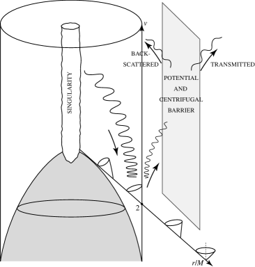
FIG. 2.: Splitting of an initial negative-frequency mode straddling the horizon into a mode falling into the black hole, and an outgoing mode which, after being partially reflected back into the black hole by the potential barrier representing gravitational and centrifugal effects, ends up as positive-frequency Hawking radiation at infinity. The antiparticle mode falling into the black hole can be interpreted as a particle travelling backwards in time, from the singularity down to the horizon [25] (hence the downwards orientation of the arrow).

The formula (47) exhibits, in the simple case of a Schwarzschild black hole, the Hawking phenomenon: a black hole radiates as if it were a black body of temperature $T_{\rm BH}=1/(8\pi M)$, covered up by a “blanket” with transmission factor $\Gamma_{\ell}(\omega)$. [The blanket being due to the effect of the potential $V_{\ell}(r)$ in Eq. (37), i.e. physically to the combined effect of gravitational attraction and centrifugal forces on the waves outgoing from the horizon.] For a Schwarzschild black hole the surface gravity is $\kappa=GM/r_{S}^{2}=1/(4M)$ (with $c=G=1$), so that the Planck spectrum present in (47) agrees with the temperature (29). Note that the technical origin of a Planck spectrum with temperature $1/8\pi M$ is the logarithm $-4M\ln((r-2M)/2M)$ in Eq. (40) which is itself linked to the logarithm $+2M\ln((r-2M)/2M)$ in Eq. (36). In other words, it is the logarithmically divergent link between the coordinate time of a local freely falling frame near ${\mathcal{H}}$ and the time at infinity which is the source of a Planck spectrum. Note that the calculation above technically relies on using such a logarithmically divergent link between the negative-frequency wave-packet near the horizon, and the positive-frequency wave-packet at infinity. When considering finite-frequency packets at infinity, this formally means that one has worked with packets containing arbitrarily high frequencies near the horizon.

When generalizing the analysis to a general black hole, one finds that the factor $4M$ gets replaced by the inverse of the surface gravity of the hole. One then finds a Planck-like spectrum containing (for bosons), besides a grey-body factor $\Gamma$, a factor $(e^{2\pi(\omega-p_{\varphi}\Omega-e\Phi)/\kappa}-1)^{-1}$ exhibiting the combined effect of the general temperature (29) and of the couplings of the conserved angular momentum $p_{\varphi}$ and electric charge $e$ to, respectively, the angular velocity $\Omega$ and electric potential $\Phi$ of the hole, see Eq. (21).

Numerically, $T_{\rm BH}\sim 10^{-6}\,K\,M_{\odot}/M$ so that Hawking’s radiation is not astrophysically relevant for stellar-mass or larger black holes. Conceptually, it is, however, a beautiful discovery which connects relativistic gravity and quantum mechanics.

IV Black holes, quantum mechanics and string theory

A Conceptual puzzles

The discovery of Hawking radiation led to new conceptual challenges. First, the obtention of a Planck-like spectrum with the temperature (29) fixed the dimensionless coefficient $\hat{\alpha}$ in the general form (28) to the value $\hat{\alpha}=\frac{1}{4}$. By the general “first law of black-hole thermodynamics” (21) this would then correspond to an entropy (27) with the same value of $\hat{\alpha}$, i.e.

$$S_{\rm BH}=\frac{1}{4}\,\frac{c^{3}}{\hbar G}\,A\equiv\frac{1}{4}\,\frac{A}{\ell_{P}^{2}}\,.$$ (48)

However, Hawking’s derivation of a temperature does not help in understanding the physical meaning of the Bekenstein-Hawking “entropy” (48). Beyond the original hints of Bekenstein that $S_{\rm BH}$ is a measure of the information loss about what went into the black hole, it remains the challenge of interpreting in a precise way $S_{\rm BH}$, à la Boltzmann, as the logarithm of the number of quantum micro-states of a macroscopic black hole.

Another challenge comes from considering the end-point of the Hawking quantum evaporation process. In order of magnitude (and in units $c=\hbar=G=1$), Hawking’s radiation corresponds to an outgoing flux of energy of order (by Stephan’s law) $\sim AT_{\rm BH}^{4}\sim R_{\rm BH}^{2}\,T_{\rm BH}^{4}\sim M^{2}\,M^{-4}\sim M^{-2}$. This loss should correspond to a secular decrease of the mass $M$ of the black hole so that $dM/dt\sim-M^{-2}$, i.e. $M^{3}\sim M_{0}^{3}-(t-t_{0})$. This leads to a finite evaporation lifetime for a black hole of order

$$t_{\rm evap}\sim t_{P}\left(\frac{M}{M_{P}}\right)^{3}\sim 10^{-44}s\left(\frac{M}{10^{-5}g}\right)^{3}\sim 10^{10}{\rm yr}\left(\frac{M}{10^{14}g}\right)^{3}$$ (49)

where $t_{P}\equiv(\hbar G/c^{5})^{1/2}\simeq 5.4\times 10^{-44}s$ is the Planck time and $M_{P}\equiv(\hbar c/G)^{1/2}\simeq 2.2\times 10^{-5}g$ the Planck mass. Besides the (remote) astrophysical possibility [25] of seing today in the sky the explosions of black holes of initial mass $M\sim 10^{14}g$ formed in the big bang, the main consequence of the finiteness of the evaporation time (49) is to oblige us to face the following questions: (i) what is the end point of the evaporation process?, and (ii) is there an “information loss” paradox due to the eventual final disappearance of the part of the wave packets in Fig. 2 which fell into the hole, and the concomitant emission of an outgoing flux of uncorrelated thermal radiation. Hawking suggested [37] that if the quantum radiance phenomenon ultimately leads to the disappearance of the black hole, then the information about what has fallen in is completely lost, and one must describe the evaporation process by a density matrix rather than by a unitary quantum evolution. In addition, we saw above that the calculation of the Hawking process formally involved arbitrarily high frequencies near the horizon. Many authors felt uncomfortable about this intermediate use of arbitrarily high (so-called “trans-Planckian”) frequencies. A lot of work was devoted to these issues, as well as to the issue of understanding the statistical meaning of the Bekenstein-Hawking entropy.

We will not try here to summarize all the work done on these issues. Let us mention the existence of various lines of work, and give entries to the literature. Several authors explored the possibility that quantum black holes have a discrete mass spectrum, e.g. with the area $A=16\pi M_{\rm irr}^{2}$ having an uniformly spaced spectrum of eigenvalues $\frac{1}{4}\,A=\ell_{P}^{2}(n+{\rm cst.})$. Then, to give a statistical meaning to the entropy $S_{\rm BH}$ one needs to assume that each discrete energy level $A_{n}$ has a huge degeneracy $g_{n}=\exp\left(\frac{1}{4}\,A_{n}/\ell_{P}^{2}\right)$. See Refs. [28, 29, 30, 31, 32]. Some authors have tried to identify the microstates responsible for black-hole entropy as near-horizon excitations [33, 34, 35, 36]. For entries in the literature on the “black-hole information puzzle”, see [37, 38, 39, 40, 41, 42]. For discussions of the insensitivity of the Hawking process to the arbitrarily high frequencies that seem to play a crucial role in all its derivations, see [43, 44, 45, 46]. For suggestions that the so-called Loop Quantum Gravity may account for black-hole entropy see [47, 48]. For a possible link between black-hole entropy and the quasinormal modes of black holes see [49, 50, 51]. Finally, let us mention the suggestion of a (black-hole motivated) upper bound, on the entropy of any system, of the form $S<\beta ER/\hbar c$, where $\beta$ is a constant of order unity, $E$ the energy of the system, and $R$ its (effective) radius [52]. See, however, [53] and references therein, for a discussion of possible loopholes in this, and other (“holographic”-type) entropy bounds.

B Extremal black holes and supersymmetric solitonic states in string theory

1 BPS extremal black holes and D branes

Here we shall focus on the most striking “explanation” of black-hole entropy, which was obtained within the framework of string theory. For early suggestions of a link between black-hole entropy and “string entropy” (i.e. the huge degeneracy of very massive string states) see [54, 55, 56]. After a seminal paper of Sen [57], a breakthrough was brought by the works of Strominger and Vafa [58] and Callan and Maldacena [59]. These works on the microscopic origin of the Bekenstein-Hawking entropy of certain (Bogomolnyi-Prasad-Sommerfield; BPS) extremal black holes initiated a huge activity, which is reviewed in [60, 61]. For textbook reviews see section 14.8 in volume 2 of [62] and chapter 17 of [63] (see also [64] for an entry into the literature on stringy black holes).

The line of work just mentioned on the micro-structure of certain BPS extremal black holes has led to very beautiful results. The factor $\frac{1}{4}$  in the entropy (48) has been verified in the explicit counting of the degeneracy of some extremal black holes, and one could also verify some aspects of the physics of near-extremal holes, such as explaining Hawking radiation as a process of quantum decay of some unstable states [59, 66], and even verifying the presence of the correct grey-body factor $\Gamma_{\ell}(\omega)$ in Eq. (47) (at least in the long-wavelength limit) [67, 68]. Note that the Hawking temperature (29), being proportional to the surface gravity $\kappa$, Eq. (23), vanishes in the limit of extremal black holes, i.e. black holes saturating the inequality (10). [The BPS black holes automatically saturate this inequality.] One therefore expects any quantum representation of an extremal black hole to be a stable (non radiating) object. This is the case of the supersymmetric BPS states studied in the above references. Then, allowing for a small deviation from the BPS condition, and therefore a small deviation from extremality, is expected to lead to a weakly unstable object, which can be treated by perturbation theory. [Even so, the problem is more tricky than was first thought [61].] Let us also mention that the study of extremal BPS black holes in certain limits led Maldacena [69] to conjecture a correspondence between string theory in anti-de-Sitter (AdS) spacetimes (times a compact manifold) and certain Conformal Field Theories (CFT). In turn, the study of this correspondence led to new insights into black-hole physics and to a confirmation that the black-hole evaporation process should be describable as a unitary process in quantum mechanics (see [70] for a review).

However, in spite of its striking successes the work on the string-theory modelling of BPS black holes has some drawbacks and limitations. The main point is that this approach describes the quantum micro-structure of BPS black holes in terms of a (nearly non-interacting) gas of massive, charged string solitons, called “Dirichlet branes”, or simply $D$-branes [71, 62]. For a recent extensive review of $D$-branes see [63]. These solitons come in various dimensionalities: a $D$-$p$ brane denotes a $D$-brane which is extended in $p$ spatial dimensions, e.g. a $D$-0 brane denotes a Dirichlet point particle, while a $D$-1 brane denotes a Dirichlet string. These solitons carry “Ramond-Ramond” charges, i.e. they create electric-like or magnetic-like $p^{\prime}$-form fields called Ramond-Ramond fields. [$p^{\prime}$-form fields are generalizations of Maxwell fields: instead of a (one-index) vector potential $A_{\mu}$, now called a 1-form field, one considers $p^{\prime}$-index antisymmetric potentials $A_{\mu_{1}\cdots\mu_{p^{\prime}}}$. In a $\cal D$-dimensional spacetime, a $D$-$p$ brane naturally couples to an electric-like $(p+1)$-form field, or to a magnetic-like $({\cal D}-p-3)$-form field.]

Roughly speaking the interaction between these solitons vanishes because of a cancellation between gravitational attraction and electrostatic repulsion. [Recall that the non-spinning limit of the extremality constraint (10) yields $|Q|=G^{\frac{1}{2}}M$ which corresponds exactly to the pairwise cancellation between $-\,GM_{1}M_{2}/r^{d-2}$ and $+\,Q_{1}Q_{2}/r^{d-2}$ in space dimension $d$ .] Because of the BPS condition (which requires the preservation of part of the original maximal supersymmetry), the classical cancellation just mentioned extends also to quantum cancellations between couplings involving bosonic fields and couplings involving fermionic ones. These quantum cancellations then entail the existence of certain non-renormalization theorems, stating that certain, specific quantities do not depend on the value of the string coupling constant, say $g$. In turn, these non-renormalization theorems are crucial to the whole enterprise because of the following fact, that I have not yet spelled out. All the string calculations of supposedly “black hole” properties (such as the degeneracy of micro-states or the decay rate of nearly-BPS states) actually refer to a system of $D$-brane solitons in the limit $g\to 0$ where these solitons admit a string-theory description. Roughly speaking, the mass of those solitons scale like $g^{-1}$, while the gravitational constant scales like $g^{2}$. Therefore the $g\to 0$ limit corresponds to a limit where the product $GM\propto g$ tends to zero, which means physically that the “Schwarzschild radius” of the considered assembly of (nearly coincident) $D$-branes is much smaller than the string length $\ell_{s}\sim\sqrt{\alpha^{\prime}}$. This is the limit where the assembly of $D$-branes is physically a “point particle”, rather than a classically describable “black hole”, having an horizon much larger than $\ell_{s}$.

2 The example of $D$-1–$D$-5 branes in type IIB string theory

One of the most studied system is a configuration of $N_{1}$ $D$-1 branes and $N_{5}$ $D$-5 branes in type IIB string theory, carrying some momentum along the direction of the $D$-1 branes (which are all parallel to each other and embedded within the $D$-5 branes). One compactifies, à la Kaluza-Klein, the 5 spatial dimensions along which lie the $D$-5 and the $D$-1 branes. More precisely, the compactified manifold is $T^{4}\times S^{1}$ where the 4-torus $T^{4}$ has volume $(2\pi)^{4}V$ and the circle $S^{1}$ has length $2\pi R$. This has the effect of quantizing the (internal) momentum moving along the branes, say $P=N\hbar/R$, where $R$ is the compactified radius along the $D$-1 direction. Finally, the configuration appears as being “point-like” in the 4 remaining uncompactified spatial dimensions, and this “point” carries three types of charges (quantized in integers): $N_{1},N_{5}$ and $N$. The total mass-energy of the configuration reads (in string units $\alpha^{\prime}=1$)

$$M=\frac{N_{1}R}{g}+\frac{N_{5}RV}{g}+\frac{N}{R}\,.$$ (50)

$D$-brane techniques (together with the general Cardy formula [72] giving the density of states in two-dimensional conformal field theory) allow one to evaluate the quantum degeneracy $\cal D$ of the (supersymmetric) ground state of this system of $D$-1 and $D$-5 branes [58, 59, 61]. Indeed, though the full structure of those solitons cannot be described by perturbative string theory, one can describe, in the limit $g\to 0$ where the $D$-branes become infinitely massive, the excitations of collections of $D$-branes in terms of (perturbative) open strings whose end points are constrained to move on the (nearly fixed) $D$-brane submanifolds [71, 62, 63]. In the considered case, one finds that the excitations of the $D$-1, $D$-5 brane configuration are described by a two-dimensional superconformal field theory with $4N_{1}N_{5}$ real scalars and, by supersymmetry, $4N_{1}N_{5}$ Majorana fermions. This yields a central charge $c=6N_{1}N_{5}$ for a system of left-movers with $L_{0}$ level given by $N$. The general Cardy formula ${\cal D}(N)\sim\exp(2\pi\sqrt{cN/6})$ (asymptotically valid for large values of $N$; see [73] for power-law corrections to the general exponential Cardy formula) then gives the following result for the quantum degeneracy of the $D$-brane configuration

$${\cal D}\sim e^{2\pi\sqrt{N_{1}N_{5}N}}\,,$$ (51)

which will be compared below to the degeneracy of the corresponding black hole expected from the Bekenstein-Hawking entropy.

At some larger value of $g$ one expects the collection of $D$-branes to smoothly turn into a quasi-classical black hole. However, the present state of development of string theory does not allow one to explicitly study this transition, and to set up a well-defined quantum Hilbert-space description of quasi-classical black holes. One has to crucially rely on non-renormalization theorems to “blindly” continue the result of calculations well-defined as $g\to 0$ into physical properties of quasi-classical black holes (such as the degeneracy of a certain quantum BPS state which is explicitly describable when $g\to 0$, but whose “physical form” for larger $g$ cannot be concretely described as a quantum state). For instance, the $D$-1 $D$-5 system mentioned above is expected to appear, when $g$ (or rather some effective value of $g$, say $g_{\rm eff}$, which is a combination of $g$ and of the integers $N_{1},N_{5},N$) gets larger than one, as a (BPS) black hole, i.e. a generalization of the extremal Reissner-Nordstrøm black hole ($G^{1/2}M=|Q|$), carrying the (conserved) quantized charges $N_{1},N_{5},N$. In other words, when $g_{\rm eff}$ gets large one can no longer describe this system of massive solitons as a “point charge”, because the combined gravitational effect of the total mass of the soliton configuration, and of the mass-energy associated to the various Ramond-Ramond (and internal-momentum related) fields it creates, generates a strong curvature of space around it, and ultimately gives birth to a finite area horizon, instead of a “point with nothing inside it”. For instance, the $(4+1)$-dimensional (Einstein-frame) metric generated, in the uncompactified dimensions, by a $D$-1 $D$-5 system carrying the quantized charges $N_{1}$, $N_{5}$, $N$, reads

$$ds_{E}^{2}=-(f_{1}\,f_{5}\,f)^{-\frac{2}{3}}\,dt^{2}+(f_{1}\,f_{5}\,f)^{\frac{1}{3}}\,(dx_{1}^{2}+\ldots+dx_{4}^{2})\,,$$ (52)

with

$$f_{1}=1+\frac{4GR}{g\pi\alpha^{\prime}}\,\frac{N_{1}}{r^{2}}\,,\ f_{5}=1+\alpha^{\prime}g\,\frac{N_{5}}{r^{2}}\,,\ f=1+\frac{4G}{\pi R}\,\frac{N}{r^{2}}\,,$$ (53)

where $r^{2}\equiv x_{1}^{2}+\ldots+x_{4}^{2}$ denotes a (squared) radial coordinate in the 4 uncompactified spatial dimensions. See references [59, 60, 61, 62, 63] for the explicit form of the other fields generated by a system of coincident $D$-branes. We shall content ourselves here with illustrating the evolution, with $g$, of the physical structure of a system of coincident $D$-branes in Fig. 3.

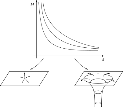
FIG. 3.: Evolution of the mass-energy, and of the physical structure, of an initially point-like configuration of $D$-branes as the string coupling $g$ increases.

The resulting extremal black hole is uniquely characterized by the knowledge of the conserved quantized charges $N,N_{1},N_{5}$. In particular, the horizon of the black-hole metric (52) is located at the radial coordinate $r=0$. [Note that, as $r\to 0$, the time-time component of the metric (52) is proportional to $((r^{-2})^{3})^{-\frac{2}{3}}=r^{+4}$.] The “area” (which is that of a 3-dimensional sphere) of the black-hole horizon is finite, because $(f_{1}\,f_{5}\,f)^{\frac{1}{3}}\propto r^{-2}$ compensates the factor $r^{2}$ in the non-radial part of the spatial metric $r^{2}\,d\,\Omega_{3}^{2}$. It is an easy matter to evaluate this “area”, and thereby, using formula Eq.(48) above, the corresponding Bekenstein-Hawking entropy. One finds that the dependences on $G$, $R$, $g$ and $\alpha^{\prime}$ cancell out so that the latter entropy depends only on the quantized charges carried by the BPS black hole, and equals

$$S_{BH}=2\pi\sqrt{N_{1}N_{5}N}\,,$$ (54)

which exactly coincides with the logarithm of the $D$-brane degeneracy Eq.(51).

C Schwarzschild black holes and string states

1 String–black-hole transition and conjectured correspondence between string and black-hole states

Because of the drawback of not being able to follow in detail the “transformation” between a point-like system of $D$-branes and a black hole, we shall focus henceforth on another type of string-theory calculation of the properties of massive string states and on their transition to black-hole states [74, 75, 76]. As just said, most of the stringy literature has concentrated on some special, supersymmetric extremal black holes (BPS black holes). These black holes carry special (Ramond-Ramond) charges and their microscopic structure seem to be describable (when $g^{2}<g_{c}^{2}$) in terms of Dirichlet-branes. By contrast, we consider here the simplest, Schwarzschild black holes (in any space dimension $d$). It will be argued that their “microscopic structure” at low $g^{2}$ involves only fundamental string states (instead of solitonic string states, such as $D$-branes). However, the lack of supersymmetry means that it becomes essential to deal with self-gravity effects.

To start with, let us recall that thirty years ago the study of the spectrum of string theory revealed [77] a huge degeneracy of states growing as an exponential of the mass. This string result was obtained a few years before Bekenstein [21] proposed that the entropy of a black hole should be proportional to the area of its horizon in Planck units, and Hawking [26] fixed the constant of proportionality after discovering that black holes do emit thermal radiation at a temperature $T_{\rm Haw}\sim R_{\rm BH}^{-1}$.

When string and black-hole entropies are compared one immediately notices a striking difference: string entropy is proportional to the first power of mass in any number of spatial dimensions $d$, while black-hole entropy is proportional to a $d$-dependent power of the mass, always larger than $1$. In formulae:

$$S_{s}\sim{\alpha^{\prime}M\over\ell_{s}}\sim M/M_{s}~{}~{}~{}~{},~{}~{}~{}~{}~{}~{}S_{\rm BH}\sim\frac{{\rm Area}}{G}\sim\frac{R_{\rm BH}^{d-1}}{G}\sim\frac{(g^{2}\,M/M_{s})^{\frac{d-1}{d-2}}}{g^{2}}\;,$$ (55)

where, as usual, $\alpha^{\prime}$ is the inverse of the classical string tension, $\ell_{s}\sim\sqrt{\alpha^{\prime}\hbar}$ is the quantum length associated with it, $M_{s}\sim\sqrt{\hbar/\alpha^{\prime}}$ is the corresponding string mass scale, $R_{\rm BH}$ is the Schwarzschild radius associated with $M$:

$$R_{\rm BH}\sim(G\,M)^{1/(d-2)}\;,$$ (56)

and we have used that, at least at sufficiently small coupling, the Newton constant and $\alpha^{\prime}$ are related via the string coupling by

$$G\sim g^{2}(\alpha^{\prime})^{(d-1)/2}$$ (57)

(or more geometrically, $\ell_{P}^{d-1}\sim g^{2}\ell_{s}^{d-1}$).

Given their different mass dependence, it is obvious that, for a given set of the fundamental constants $G,\alpha^{\prime},g^{2}$, $S_{s}>S_{\rm BH}$ at sufficiently small $M$, while the opposite is true at sufficiently large $M$. Obviously, there has to be a critical value of $M$, $M_{c}$, at which $S_{s}=S_{\rm BH}$. This observation had led Bowick et al. [54] to conjecture that large black holes end up their Hawking-evaporation process when $M=M_{c}$, and then transform into a higher-entropy string state without ever reaching the singular zero-mass limit. This reasoning is confirmed [55] by the observation that, in string theory, the fundamental string length $\ell_{s}$ should set a minimal value for the Schwarzschild radius of any black hole (and thus a maximal value for its Hawking temperature). It was also noticed [54, 56, 78] that, precisely at $M=M_{c}$, $R_{\rm BH}=\ell_{s}$ and the Hawking temperature equals the Hagedorn temperature of string theory. For any $d$, the value of $M_{c}$ is given by:

$$M_{c}\,\sim M_{s}g^{-2}\,.$$ (58)

Susskind and collaborators [56, 79] went a step further and proposed that the spectrum of black holes and the spectrum of single string states be “identical”, in the sense that there be a one to one correspondence between (uncharged) fundamental string states and (uncharged) black-hole states. Such a “correspondence principle” has been generalized by Horowitz and Polchinski [74] to a wide range of charged black-hole states (in any dimension). Instead of keeping fixed the fundamental constants and letting $M$ evolve by evaporation, as considered above, one can (equivalently) describe the physics of this conjectured correspondence by following a narrow band of states, on both sides of and through, the string $\rightleftharpoons$ black hole transition, by keeping fixed the entropy $S=S_{s}=S_{\rm BH}$, while adiabatically varying the string coupling $g$, i.e. the ratio between $\ell_{P}$ and $\ell_{s}$. The correspondence principle then means that if one increases $g$ each (quantum) string state should turn into a (quantum) black-hole state at sufficiently strong coupling, while, conversely, if $g$ is decreased, each black-hole state should “decollapse” and transform into a string state at sufficiently weak coupling. For all the reasons mentioned above, it is very natural to expect that, when starting from a black hole state, the critical value of $g$ at which a black hole should turn into a string is given, in clear relation to (58), by

$$g_{c}^{2}\,M\sim M_{s}\,,$$ (59)

and is related to the common value of string and black-hole entropy via

$$g_{c}^{2}\sim\frac{1}{S_{\rm BH}}=\frac{1}{S_{s}}\;.$$ (60)

Note that $g_{c}^{2}\ll 1$ for the very massive states ($M\gg M_{s}$) that we consider. This justifies our use of the perturbative relation (57) between $G$ and $\alpha^{\prime}$.

As we said above, in the case of extremal BPS, and nearly extremal, black holes the conjectured correspondence was dramatically confirmed through the work of Strominger and Vafa [58] and others [57, 59, 61] leading to a statistical mechanics interpretation of black-hole entropy in terms of the number of microscopic states sharing the same macroscopic quantum numbers. However, little is known about whether and how the correspondence works for non-extremal, non BPS black holes, such as the simplest Schwarzschild black hole. By contrast to BPS states whose mass is protected by supersymmetry, we shall consider here the effect of varying $g$ on the mass and size of non-BPS string states.

Although it is remarkable that black-hole and string entropy coincide when $R_{\rm BH}=\ell_{s}$, this is still not quite sufficient to claim that, when starting from a string state, a string becomes a black hole at $g=g_{c}$. In fact, the process in which one starts from a string state in flat space and increases $g$ poses a serious puzzle [56]. Indeed, the radius of a typical excited string state of mass $M$ is generally thought of being of order

$$R_{s}^{\rm rw}\sim\ell_{s}(M/M_{s})^{1/2}\,,$$ (61)

as if a highly excited string state were a random walk made of $M/M_{s}=\alpha^{\prime}M/\ell_{s}$ segments of length $\ell_{s}$ [80]. [The number of steps in this random walk is, as is natural, the string entropy (55).] The “random walk” radius (61) is much larger than the Schwarzschild radius for all couplings $g\leq g_{c}$, or, equivalently, the ratio of self-gravitational binding energy to mass (in $d$ spatial dimensions)

$$\frac{G\,M}{(R_{s}^{\rm rw})^{d-2}}\sim\left(\frac{R_{\rm BH}(M)}{R_{s}^{\rm rw}}\right)^{d-2}\sim g^{2}\left(\frac{M}{M_{s}}\right)^{\frac{4-d}{2}}$$ (62)

remains much smaller than one (when $d>2$, to which we restrict ourselves) up to, and including, the transition point. In view of (62) it does not seem natural to expect that a string state will “collapse” to a black hole when $g$ reaches the value (59). One would expect a string state of mass $M$ to turn into a black hole only when its typical size is of order of $R_{\rm BH}(M)$ (which is of order $\ell_{s}$ at the expected transition point (59)). According to Eq. (62), this seems to happen for a value of $g$ much larger than $g_{c}$.

Horowitz and Polchinski [75] have addressed this puzzle by means of a “thermal scalar” formalism [81]. Their results suggest a resolution of the puzzle when $d=3$ (four-dimensional spacetime), but lead to a rather complicated behaviour when $d\geq 4$. Moreover, even in the simple $d=3$ case, the formal nature of the auxiliary “thermal scalar” renders unclear (at least to me) the physical interpretation of their analysis. In the next section, I will review the results of Ref. [76] whose aim was to clarify the string $\rightleftharpoons$ black-hole transition by a direct study, in real spacetime, of the size and mass of a typical excited string, within the microcanonical ensemble of self-gravitating strings.

2 A microcanonical approach to self-gravitating strings

The results of [76] lead to a rather simple picture of the transition, in any dimension. Let us summarize them before entering into the technical details of the analysis.

The critical value for the transition is (59), or (60) in terms of the entropy $S$, for both directions of the string $\rightleftharpoons$ black hole transition. In three spatial dimensions, one finds that the size (computed in real spacetime) of a typical self-gravitating string is given by the random walk value (61) when $g^{2}\leq g_{0}^{2}$, with $g_{0}^{2}\sim(M/M_{s})^{-3/2}\sim S^{-3/2}$, and by

$$R_{\rm typ}\sim\frac{1}{g^{2}\,M}\,,$$ (63)

when $g_{0}^{2}\leq g^{2}\leq g_{c}^{2}$. Note that $R_{\rm typ}$ smoothly interpolates between $R_{s}^{\rm rw}$ and $\ell_{s}$. This result confirms the picture proposed by Ref. [75] when $d=3$, but with the bonus that Eq. (63) refers to a radius which is estimated directly in physical space (see below), and which is the size of a typical member of the microcanonical ensemble of self-gravitating strings. In all higher dimensions, we find that the size of a typical self-gravitating string remains fixed at the random walk value (61) when $g\leq g_{c}$. However, when $g$ gets close to a value of order $g_{c}$, the ensemble of self-gravitating strings becomes (smoothly in $d=4$, but suddenly in $d\geq 5$) dominated by very compact strings of size $\sim\ell_{s}$ (which are then expected to collapse with a slight further increase of $g$ because the dominant size is only slightly larger than the Schwarzschild radius at $g_{c}$). The results of [76] confirm and clarify the main idea of a correspondence between string states and black hole states [56, 79, 74, 75], and suggest that the transition between these states is rather smooth, symmetrical with no apparent “hysteresis effect”, and with continuity in entropy, mass, typical size, and luminosity. It is, however, beyond the technical grasp of this analysis to compute any precise number at the transition (such as the famous factor $1/4$ in the Bekenstein-Hawking entropy formula). Let us now enter into some of the technical details.

For simplicity, we deal with open bosonic strings ($\ell_{s}\equiv\sqrt{2\,\alpha^{\prime}}$, $0\leq\sigma\leq\pi$)

$$X^{\mu}(\tau,\sigma)=X_{\rm cm}^{\mu}(\tau,\sigma)+\widetilde{X}^{\mu}(\tau,\sigma)\,,$$ (64)

$$X_{\rm cm}^{\mu}(\tau,\sigma)=x^{\mu}+2\,\alpha^{\prime}\,p^{\mu}\,\tau\,,$$ (65)

$$\widetilde{X}^{\mu}(\tau,\sigma)=i\,\ell_{s}\sum_{n\not=0}\ \frac{\alpha_{n}^{\mu}}{n}\ e^{-in\tau}\,\cos\,n\,\sigma\,.$$ (66)

Here, we have explicitly separated the center of mass motion $X_{\rm cm}^{\mu}$ (with $[x^{\mu},p^{\nu}]=i\,\eta^{\mu\nu}$) from the oscillatory one $\widetilde{X}^{\mu}$, which is expressed in terms of two parameters: the worldsheet time parameter $\tau$ and the worldsheet spatial parameter $\sigma$ ($[\alpha_{m}^{\mu},\alpha_{n}^{\nu}]=m\,\delta_{m+n}^{0}\,\eta^{\mu\nu}$). The free spectrum is given by $\alpha^{\prime}\,M^{2}=N-1$ where $(\alpha\cdot\beta\equiv\eta_{\mu\nu}\,\alpha^{\mu}\,\beta^{\nu}\equiv-\alpha^{0}\,\beta^{0}+\alpha^{i}\,\beta^{i})$

$$N=\sum_{n=1}^{\infty}\ \alpha_{-n}\cdot\alpha_{n}=\sum_{n=1}^{\infty}\ n\,N_{n}\,.$$ (67)

Here $N_{n}\equiv a_{n}^{\dagger}\cdot a_{n}$ is the occupation number of the $n^{\rm th}$ oscillator ($\alpha_{n}^{\mu}=\sqrt{n}\ a_{n}^{\mu}$,$[a_{n}^{\mu},a_{m}^{\nu\dagger}]=\eta^{\mu\nu}\,\delta_{nm}$, with $n,m$ positive).

The decomposition (64)–(66) holds in any conformal gauge ($(\partial_{\tau}\,X^{\mu}\pm\partial_{\sigma}\,X^{\mu})^{2}=0$). One can further specify the choice of worldsheet coordinates by imposing

$$n_{\mu}\,X^{\mu}(\tau,\sigma)=2\alpha^{\prime}(n_{\mu}\,p^{\mu})\,\tau\,,$$ (68)

where $n^{\mu}$ is an arbitrary timelike or null vector ($n\cdot n\leq 0$) [82]. Eq. (68) means that the $n$-projected oscillators $n_{\mu}\,\alpha_{m}^{\mu}$ are set equal to zero. As we shall be interested in quasi-classical, very massive string states ($N\gg 1$) it should be possible to work in the “center of mass” gauge, where the vector $n^{\mu}$ used in Eq. (68) to define the $\tau$-slices of the world-sheet is taken to be the total momentum $p^{\mu}$ of the string. This gauge is the most intrinsic way to describe a string in the classical limit. Using this intrinsic gauge, one can covariantly define the proper rms size of a massive string state as

$$R^{2}\equiv\frac{1}{d}\ \langle(\widetilde{X}_{\perp}^{\mu}\,(\tau,\sigma))^{2}\rangle_{\sigma,\tau}\,,$$ (69)

where $\widetilde{X}_{\perp}^{\mu}\equiv\widetilde{X}^{\mu}-p^{\mu}(p\cdot\widetilde{X})/(p\cdot p)$ denotes the projection of $\widetilde{X}^{\mu}\equiv X^{\mu}-X_{\rm cm}^{\mu}(\tau)$ orthogonally to $p^{\mu}$, and where the angular brackets denote the (simple) average with respect to $\sigma$ and $\tau$.

In the center of mass gauge, $p_{\mu}\,\widetilde{X}^{\mu}$ vanishes by definition, and Eq. (69) yields simply

$$R^{2}=\frac{1}{d}\,\ell_{s}^{2}\,{\cal R}\,,$$ (70)

with (after discarding a logarithmically infinite, but state independent, contribution)

$${\cal R}\equiv\sum_{n=1}^{\infty}\ \frac{\alpha_{-n}\cdot\alpha_{n}}{n^{2}}=\sum_{n=1}^{\infty}\ \frac{a_{n}^{\dagger}\cdot a_{n}}{n}=\sum_{n=1}^{\infty}\ \frac{N_{n}}{n}\,.$$ (71)

We wish to estimate the distribution function in size of the ensemble of free string states of mass $M$, i.e. to count the number of string states, having some fixed values of $M$ and $R$ (or, equivalently, $N$ and ${\cal R}$). An approximate estimate of this number (“degeneracy”) is [76]

$${\cal D}\,(M,R)\sim\exp\,[c\,(R)\,a_{0}\,M]\,,$$ (72)

where $a_{0}=2\,\pi\,((d-1)\,\alpha^{\prime}/6)^{1/2}$ and

$$c\,(R)=\left(1-\frac{c_{1}}{R^{2}}\right)\left(1-c_{2}\,\frac{R^{2}}{M^{2}}\right)\,,$$ (73)

with the coefficients $c_{1}$ and $c_{2}$ being of order unity in string units. The coefficient $c\,(R)$ gives the fractional reduction in entropy brought by imposing a size constraint. Note that (as expected) this reduction is minimized when $c_{1}\,R^{-2}\sim c_{2}\,R^{2}/M^{2}$, i.e. for $R\sim R_{\rm rw}\sim\ell_{s}\,\sqrt{M/M_{s}}$.

We also need to estimate the mass shift of string states (of mass $M$ and size $R$) due to the exchange of the various long-range fields which are universally coupled to the string: graviton, dilaton and axion. As we are interested in very massive string states, $M\gg M_{s}$, in extended configurations, $R\gg\ell_{s}$, we expect that massless exchange dominates the (state-dependent contribution to the) mass shift. [The exchange of spin 1 fields (for open strings) becomes negligible when $M\gg M_{s}$ because it does not increase with $M$.]

The evaluation, in string theory, of (one loop) mass shifts for massive states is technically quite involved, and can only be tackled for the states which are near the leading Regge trajectory [83]. [Indeed, the vertex operators creating these states are the only ones to admit a manageable explicit oscillator representation.] As we consider states which are very far from the leading Regge trajectory, there is no hope of computing exactly (at one loop) their mass shifts.

In Ref. [76] we could estimate the one-loop mass-shift by resorting to a semi-classical approximation. The starting point of this semi-classical approximation is the effective action of self-gravitating fundamental strings derived in Ref. [84]. Using coherent-state methods [85, 82, 86] and a generalization of Bloch’s theorem (see Eq. (3.13) of [76]) one finds

$$\delta\,M\simeq-c_{d}\,G\,\frac{M^{2}}{R^{d-2}}\,,$$ (74)

with the (positive) numerical constant

$$c_{d}=\left[\frac{d-2}{2}\,(4\pi)^{\frac{d-2}{2}}\right]^{-1}\,,$$ (75)

equal to $1/\sqrt{\pi}$ in $d=3$.

The result (74) was expected in order of magnitude, but it is important to check that it approximately comes out of a detailed calculation of the mass shift which incorporates both relativistic and quantum effects and which uses the precise definition (71) of the squared size.

Finally, let us mention that, by using the same tools Ref. [76] has computed the imaginary part of the mass shift $\delta\,M=\delta\,M_{\rm real}-i\,\Gamma/2$, i.e. the total decay rate $\Gamma$ in massless quanta, as well as the total power radiated $P$. In order of magnitude these quantities are

$$\Gamma\sim g^{2}\,M\ ,\ P\sim g^{2}\,M\,M_{s}\,.$$ (76)

Finally one combines the results above, Eqs. (72) and (74), and heuristically extend them at the limit of their domain of validity. We consider a narrow band of string states that we follow when increasing adiabatically the string coupling $g$, starting from $g=0$. Let $M_{0}$, $R_{0}$ denote the “bare” values (i.e. for $g\rightarrow 0$) of the mass and size of this band of states. Under the adiabatic variation of $g$, the mass and size, $M$, $R$, of this band of states will vary. However, the entropy $S(M,R)$ remains constant under this adiabatic process: $S(M,R)=S(M_{0},R_{0})$. We consider states with sizes $\ell_{s}\ll R_{0}\ll M_{0}$ for which the correction factor,

$$c\,(R_{0})\simeq(1-c_{1}\,R_{0}^{-2})\,(1-c_{2}\,R_{0}^{2}/M_{0}^{2})\,,$$ (77)

in the entropy

$$S(M_{0},R_{0})=c\,(R_{0})\,a_{0}\,M_{0}\,,$$ (78)

is near unity. [We use Eq. (72) in the limit $g\rightarrow 0$, for which it was derived.] Because of this reduced sensitivity of $c\,(R_{0})$ on a possible direct effect of $g$ on $R$ (i.e. $R(g)=R_{0}+\delta_{g}\,R$), the main effect of self-gravity on the entropy (considered as a function of the actual values $M$, $R$ when $g\not=0$) will come from replacing $M_{0}$ as a function of $M$ and $R$. The mass-shift result (74) gives $\delta\,M=M-M_{0}$ to first order in $g^{2}$. To the same accuracy, (74) gives $M_{0}$ as a function of $M$ and $R$:

$$M_{0}\simeq M+c_{3}\,g^{2}\,\frac{M^{2}}{R^{d-2}}=M\left(1+c_{3}\,\frac{g^{2}\,M}{R^{d-2}}\right)\,,$$ (79)

where $c_{3}$ is a positive numerical constant.

Finally, combining Eqs. (77)–(79) (and neglecting, as just said, a small effect linked to $\delta_{g}\,R\not=0$) leads to the following relation between the entropy, the mass and the size (all considered for self-gravitating states, with $g\not=0$)

$$S(M,R)\simeq a_{0}\,M\left(1-\frac{1}{R^{2}}\right)\left(1-\frac{R^{2}}{M^{2}}\right)\left(1+\frac{g^{2}\,M}{R^{d-2}}\right)\,.$$ (80)

For notational simplicity, we henceforth set to unity (by using some redefinitions and working in some suitably defined “string units”)) the coefficients $c_{1}$, $c_{2}$ and $c_{3}$. The possibility of smoothly transforming self-gravitating string states into black-hole states come from the peculiar radius dependence of the entropy $S(M,R)$. Eq. (79) exhibits two effects varying in opposite directions: (i) self-gravity favors small values of $R$ (because they correspond to larger values of $M_{0}$, i.e. of the “bare” entropy), and (ii) the constraint of being of some fixed size $R$ disfavors both small $(R\ll\sqrt{M})$ and large $(R\gg\sqrt{M})$ values of $R$. For given values of $M$ and $g$, the most numerous (and therefore most probable) string states will have a size $R_{*}(M;g)$ which maximizes the entropy $S(M,R)$. Said differently, the total degeneracy of the complete ensemble of self-gravitating string states with total energy $M$ (and no a priori size restriction) will be given by an integral (where $\Delta\,R$ is the rms fluctuation of $R$)

$${\cal D}(M)\sim\int\frac{dR}{\Delta\,R}\,e^{S(M,R)}\sim e^{S(M,R_{*})}$$ (81)

which will be dominated by the saddle point $R_{*}$ which maximizes the exponent.

The value of the most probable size $R_{*}$ is a function of $M$, $g$ and the space dimension $d$. We refer to Ref. [76] for a full treatment. Let us only indicate the results in the (actual) three-dimensional case, $d=3$. When maximizing the entropy $S(M,R)$ with respect to $R$ one finds that: (i) when $g^{2}\ll M^{-3/2}$, the most probable size $R_{*}(M,g)\sim\sqrt{M}$, (ii) when $g^{2}\gg M^{-3/2}$,

$$R_{*}(M,g)\simeq\frac{1+\sqrt{1+3\lambda^{2}}}{\lambda}$$ (82)

where $\lambda\equiv g^{2}M$.

Eq. (82) says that, when $g^{2}$ increases, and therefore when $\lambda$ increases (beyond $M^{-1/2}$) the typical size of a self-gravitating string decreases, and (formally) tends to a limiting size of order unity, $R_{\infty}=\sqrt{3}$ (i.e. of order the string length scale $\ell_{s}=\sqrt{2\alpha^{\prime}}$) when $\lambda\gg 1$. However, the fractional self-gravity $GM/R_{*}\simeq\lambda/R_{*}$ (which measures the gravitational deformation away from flat space) becomes unity for $\lambda=\sqrt{5}$ and formally increases without limit when $\lambda$ further increases. Therefore, we expect that for some value of $\lambda$ of order unity, the self-gravity of the compact string state already reached when $\lambda\sim 1$ (indeed, Eq. (82) predicts $R_{*}\sim 1$ when $\lambda\sim 1$) will become so strong that it will (continuously) turn into a black-hole state. Having argued that the dynamical threshold for the transition string $\rightarrow$ black hole is $\lambda\sim 1$, we now notice that, for such a value of $\lambda$ the entropy $S(M)=S(M,R_{*}(M))\simeq a_{0}\,M\left[1+\frac{1}{4}\,(g^{2}M)^{2}\right]$ of the string state (of mass $M$) matches the Bekenstein-Hawking entropy $S_{\rm BH}(M)\sim g^{2}\,M^{2}=\lambda M$ of the formed black hole. One further checks that the other global physical characteristics of the string state (radius $R_{*}$, luminosity $P$, Eq. (76)) match those of a Schwarzschild black hole of the same mass ($R_{\rm BH}\sim GM\sim g^{2}M\,,\,P_{\rm Hawking}\sim R_{\rm BH}^{-2}$) when $\lambda\sim 1$.

Conceptually, the main new result of the analysis summarized above concerns the most probable state of a very massive single self-gravitating string. By combining our estimates of the entropy reduction due to the size constraint, and of the mass shift we come up with the expression (80) for the logarithm of the number of self-gravitating string states of size $R$. Our analysis of the function $S(M,R)$ clarifies the correspondence [56, 79, 74, 75] between string states and black holes. In particular, our results confirm many of the results of [75], but make them (in our opinion) physically clearer by dealing directly with the size distribution, in real space, of an ensemble of string states. When our results differ from those of [75], they do so in a way which simplifies the physical picture and make even more compelling the existence of a correspondence between strings and black holes. The simple physical picture suggested by our results is the following: In any dimension, if we start with a massive string state and increase the string coupling $g$, a typical string state will, eventually, become more compact and will end up, when $\lambda_{c}=g_{c}^{2}\,M\sim 1$, in a “condensed state” of size $R\sim 1$, and mass density $\rho\sim g_{c}^{-2}$. Note that the basic reason why small strings, $R\sim 1$, dominate in any dimension the entropy when $\lambda\sim 1$ is that they descend from string states with bare mass $M_{0}\simeq M(1+\lambda/R^{d-2})\sim 2M$ which are exponentially more numerous than less condensed string states corresponding to smaller bare masses (see Fig. 4).

The nature of the transition between the initial “dilute” state and the final “condensed” one depends on the value of the space dimension $d$. In $d=3$, the transition is gradual: when $\lambda<M^{-1/2}$ the size of a typical state is $R_{*}^{(d=3)}\simeq M^{1/2}(1-M^{1/2}\,\lambda/8)$, when $\lambda>M^{1/2}$ the typical size is $R_{*}^{(d=3)}\simeq(1+(1+3\,\lambda^{2})^{1/2})/\lambda$. In $d=4$, the transition toward a condensed state is still continuous, but most of the size evolution takes place very near $\lambda=1$: when $\lambda<1$, $R_{*}^{(d=4)}\simeq M^{1/2}(1-\lambda)^{1/4}$, and when $\lambda>1$,$R_{*}^{(d=4)}\simeq(2\lambda/(\lambda-1))^{1/2}$, with some smooth blending between the two evolutions around $|\lambda-1|\sim M^{-2/3}$. In $d\geq 5$, the transition is discontinuous (like a first order phase transition between, say, gas and liquid states). Barring the consideration of metastable (supercooled) states, on expects that when $\lambda=\lambda_{2}\simeq\nu^{\nu}/(\nu-1)^{\nu-1}$ (with $\nu=(d-2)/2$), the most probable size of a string state will jump from $R_{\rm rw}$ (when $\lambda<\lambda_{2}$) to a size of order unity (when $\lambda>\lambda_{2}$).

One can think of the “condensed” state of (single) string matter, reached (in any $d$) when $\lambda\sim 1$, as an analog of a neutron star with respect to an ordinary star (or a white dwarf). It is very compact (because of self gravity) but it is stable (in some range for $g$) under gravitational collapse. However, if one further increases $g$ or $M$ (in fact, $\lambda=g^{2}\,M$), the condensed string state is expected (when $\lambda$ reaches some $\lambda_{3}>\lambda_{2}$, $\lambda_{3}={\cal O}(1)$) to collapse down to a black-hole state (analogously to a neutron star collapsing to a black hole when its mass exceeds the Landau-Oppenheimer-Volkoff critical mass). Still in analogy with neutron stars, one notes that general relativistic strong gravitational field effects are crucial for determining the onset of gravitational collapse; indeed, under the “Newtonian” approximation (80), the condensed string state could continue to exist for arbitrary large values of $\lambda$.

It is interesting to note that the value of the mass density at the formation of the condensed string state is $\rho\sim g^{-2}$. This is reminiscent of the prediction by Atick and Witten [87] of a first-order phase transition of a self-gravitating thermal gas of strings, near the Hagedorn temperature, towards a dense state with energy density $\rho\sim g^{-2}$ (typical of a genus-zero contribution to the free energy). Ref. [87] suggested that this transition is first-order because of the coupling to the dilaton. This suggestion agrees with our finding of a discontinuous transition to the single string condensed state in dimensions $\geq 5$ (Ref. [87] works in higher dimensions, $d=25$ for the bosonic case). It would be interesting to deepen these links between self-gravitating single string states and multi-string states.

Let us come back to the consequences of the picture summarized above for the problem of the end point of the evaporation of a Schwarzschild black hole and the interpretation of black-hole entropy. See Fig. 4.

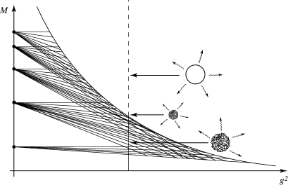
FIG. 4.: Evolution of the energy levels of massive string states as the string coupling $g$ increases. String states are expected to transform into black-hole states on the correspondence line $g^{2}M\sim M_{s}$. Vertical line: Corresponding transformation of a black hole, loosing mass at fixed $g$ under Hawking radiation, into an initially compact string state, which inflates before decaying into massless radiation.

In that case one fixes the value of $g$ (assumed to be $\ll 1$) and considers a black hole which slowly looses its mass via Hawking radiation. When the mass gets as low as a value $M\sim g^{-2}$, for which the radius of the black hole is of order one (in string units), one expects the black hole to transform (in all dimensions) into a typical string state corresponding to $\lambda=g^{2}\,M\sim 1$, which is a dense state (still of radius $R\sim 1$). This string state will further decay and loose mass, predominantly via the emission of massless quanta, with a quasi thermal spectrum with temperature $T\sim T_{\rm Hagedorn}=a_{0}^{-1}$, with $a_{0}$ defined after (72), and which smoothly matches the previous black hole Hawking temperature. This mass loss will further decrease the product $\lambda=g^{2}\,M$, and this decrease will, either gradually or suddenly, cause the initially compact string state to inflate to much larger sizes. For instance, if $d\geq 4$, the string state will quickly inflate to a size $R\sim\sqrt{M}$. Later, with continued mass loss, the string size will slowly shrink again toward $R\sim 1$ until a remaining string of mass $M\sim 1$ finally decays into stable massless quanta. In this picture, the black-hole entropy acquires a somewhat clear statistical significance (as the degeneracy of a corresponding typical string state) only when $M$ and $g$ are related by $g^{2}\,M\sim 1$. If we allow ourselves to vary (in a Gedanken experiment) the value of $g$ this gives a potential statistical significance to any black-hole entropy value $S_{\rm BH}$ (by choosing $g^{2}\sim S_{\rm BH}^{-1}$). We do not claim, however, to have a clear idea of the direct statistical meaning of $S_{\rm BH}$ when $g^{2}\,S_{\rm BH}\gg 1$. Neither do we clearly understand the fate of the very large space (which could be excited in many ways) which resides inside very large classical black holes of radius $R_{\rm BH}\sim(g^{2}\,S_{\rm BH})^{1/(d-1)}\gg 1$. The fact that the interior of a black hole of given mass could be arbitrarily large, and therefore arbitrarily complex, suggests that black-hole physics is not exhausted by the idea (discussed here) of a reversible transition between string-length-size black holes and string states.

On the string side, we also do not clearly understand how one could follow in detail (in the present non BPS framework) the “transformation” of a strongly self-gravitating string state into a black-hole state.

Finally, let us note that we expect that self-gravity will lift nearly completely the degeneracy of string states. [The degeneracy linked to the rotational symmetry, i.e. $2J+1$ in $d=3$, is probably the only one to remain, and it is negligible compared to the string entropy.] Therefore we expect (contrary to what is assumed in many works [28, 29, 30, 31, 32, 49, 50]) that the separation $\delta\,E$ between subsequent (string and black-hole) energy levels will be exponentially small: $\delta\,E\sim\Delta\,M\,\exp(-S(M))$, where $\Delta\,M$ is the canonical-ensemble fluctuation in $M$. See Fig. 4 which sketches how self-gravity (which depends on the “size” of the considered massive string state) lifts the degeneracy of free string states, and is expected to lead to a very high density of (nearly non-degenerate) energy levels. [This picture of the level structure of non-supersymmetric string/black-hole states should be contrasted with the case of supersymmetric BPS $D$-brane/black-hole states, which features well-separated discrete levels having exponentially large degeneracies. See Fig. 3 and Eq. (50).] Such a $\delta\,E$ is negligibly small compared to the radiative width $\Gamma\sim g^{2}\,M$ of the levels. This seems to mean that the discreteness of the quantum levels of strongly self-gravitating strings and black holes is very much blurred, and difficult to see observationally. Such exponentially small $\delta E$ is also expected to play an important role in “explaining” why sufficiently massive string states behave as a thermal state (see, in this respect, the recent discussion [88] of the “self-thermalization” of pure states).

V Conclusions

We hope that this short review has allowed the reader to grasp the richness of the issue of black-hole entropy. Thirty years after the original proposal of Bekenstein and the discovery by Hawking of the quantum radiance of black holes, the issue remains somewhat cloudy. String theory has brought very significant progress by allowing one to interpret the microscopic degrees of freedom of certain extremal (supersymmetric) black holes in terms of a sort of “analytic continuation in the string coupling $g$” of systems of very massive, (Ramond-Ramond) charged string solitons (Dirichlet branes). However, it is frustrating that the $D$-brane description does not apply to the regime of large (effective) string coupling $g$ where these systems are believed to “transform into” black holes. We have sketched the limited progress made in string theory for understanding the microscopic degrees of freedom of non extremal (non supersymmetric) black holes, and, in particular, the simplest Schwarzschild ones. A plausible picture emerged of a reversible transformation between Schwarzschild black-hole states (when $g^{2}M\gtrsim M_{s}$) into self-gravitating massive string states (when $g^{2}M\lesssim M_{s}$). However, the lack of supersymmetry for such states limits the secure applicability of present string technology to the regime $g^{2}M\ll M_{s}$. The extension of the results to $g^{2}M\sim M_{s}$ is physically plausible but not technically justified. In addition, all stringy calculations fail to give a precise Hilbert-space description of the microscopic structure of black holes in the regime ($g^{2}M\gg M_{s}$, or its BPS equivalent) where the considered “internal structure” has become a large, quasi-classical black hole. In particular, the quantum description of the large spacetime region constituting the interior of a quasi-classical black hole (see Fig. 1), and of all the excitations it contains (such as the “lost” parts of the Hawking particle creation phenomenon), remain somewhat mysterious (see [89] for a recent attempt at describing the quantum state of a quasi-classical black hole in a unitary way). Clearly the issue of black-hole entropy will continue to exercize the sagacity of many researchers for many years to come, and will continue to provide one of our few handles on the physics of quantum relativistic gravity, i.e. the domain where $\hbar$, $c$ and $G$ all play important roles.

Appendix

Here is an excerpt from John Wheeler’s book [22] about the genesis of the discovery of the concept of black-hole entropy by Jacob Bekenstein:

“One afternoon in 1970 Bekenstein–then a graduate student–and I were discussing black-hole physics in my office in Princeton’s Jadwin Hall. I told him the concern I always feel when a hot cup of tea exchanges heat energy with a cold cup of tea. By allowing that transfer of heat I do not alter the energy of the universe, but I do increase its microscopic disorder, its information loss, its entropy. The entropy of the world always increases in an irreversible process like that.

“The consequence of my crime, Jacob, echo down to the end of time,” I noted. “But if a black hole swims by, and I drop the teacups into it, I conceal from all the world the evidence of my crime. How remarkable!”

Bekenstein, a man of deep integrity, takes the lawfulness of creation as a matter of utmost seriousness. Several months later, he came back with a remarkable idea. “You don’t destroy entropy when you drop those teacups into the black hole. The black hole already has entropy, and you only increase it!”

Bekenstein went on to explain that the surface area of a black hole is not only analogous to entropy, it is entropy, and the surface gravity of a black hole (measured, for example, by the downward acceleration of a rock as it crosses the horizon) is not only analogous to temperature, it is temperature. A black hole is not totally cold!…”

REFERENCES

- [1] K. Schwarzschild, “ On the gravitational field of a masspoint according to Einstein’s theory” (in German), Sitzungsber. Preuss. Akad. Wiss. Berlin (Math. Phys.) 1916, 189 (1916); for an English translation see arXiv:physics/9905030.
- [2] C. DeWitt and B.S. DeWitt, eds., Black Holes (Les Houches 1972) Gordon and Breach, New York, 1973.
- [3] S.W. Hawking and G.F.R. Ellis, The large scale structure of space time, Cambridge U. Press, Cambridge, 1973.
- [4] C.W. Misner, K.S. Thorne and J.A. Wheeler, Gravitation, Freeman, San Francisco, 1972.
- [5] R.M. Wald, General Relativity, Chicago U. Press, Chicago, 1984.
- [6] M. Heusler, Black Hole Uniqueness Theorems, Cambridge U. Press, Cambridge, 1996.
-
[7]
R. Penrose, Rivista Nuovo Cimento 1, 252 (1969);
R. Penrose and R.M. Floyd, Nature 229, 177 (1971). - [8] D. Christodoulou, Phys. Rev. Lett. 25, 1596 (1970).
- [9] D. Christodoulou and R. Ruffini, Phys. Rev. D4, 3552 (1971).
- [10] S.W. Hawking, in Ref. [2].
- [11] B. Carter, in Ref. [2].
- [12] J.M. Bardeen, B. Carter and S.W. Hawking, Comm. Math. Phys. 31, 161 (1973).
- [13] R. M. Wald, “The thermodynamics of black holes”, Living Rev. Relativity 4 , (2001),6. [Online article]: cited on 15 Aug 2001; http://www.livingreviews.org/lrr-2001-6.
- [14] T. Damour, Phys. Rev. D18, 3598 (1978).
- [15] R.L. Znajek, Mon. Not. R. Astr. Soc. 185, 833 (1978).
- [16] T. Damour, Thèse de Doctorat d’Etat, Université de Paris VI, January 1979; and in Proceedings of the Second Marcel Grossmann Meeting on General Relativity, ed. by R. Ruffini (North Holland, Amsterdam, 1982), pp. 587-608.
- [17] S.W. Hawking and J.B. Hartle, Comm. Math. Phys. 27, 283 (1972).
- [18] J.B. Hartle, Phys. Rev. D9, 2749 (1974).
- [19] J.D. Bekenstein, Ph. D. thesis, Princeton University, 1972.
- [20] J.D. Bekenstein, Lett. Nuovo Cimento 4, 737 (1972).
- [21] J.D. Bekenstein, Phys. Rev. D7, 2333 (1973).
- [22] J.A. Wheeler, A Journey into Gravity and Spacetime, Scientific American Library, (W.H. Freeman & Co., New York, 1990).
- [23] J.D. Bekenstein, Physics Today January 1980, pp. 24-31.
- [24] L. Brillouin, Science and Information Theory, Academic Press, New York, 1956.
- [25] S.W. Hawking, Nature 248, 30 (1974).
- [26] S.W. Hawking, Comm. Math. Phys. 43, 199 (1975).
- [27] T. Damour and R. Ruffini, Phys. Rev. D14, 332 (1976).
- [28] J.D. Bekenstein, Lett. Nuovo Cimento 11, 467 (1974).
- [29] V. Mukhanov, JETP Letters 44, 63 (1986).
- [30] I.I. Kogan, JETP Letters 44, 267 (1986); and hep-th/9412232.
- [31] M. Maggiore, Nucl. Phys. B429, 205 (1994).
- [32] J.D. Bekenstein, gr-qc/9710076, in Proceedings of the 8th Marcel Grossmann Meeting, ed. T. Piran,(World Scientific, 1988), p. 92.
- [33] W.H. Zurek and K.S. Thorne, Phys. Rev. Lett. 54, 2171 (1985).
- [34] S. Carlip, Phys. Rev. D 51, 632 (1995).
- [35] A. Strominger, J. High Energy Phys. 2, 009 (1998).
- [36] S. Carlip, Phys. Rev. Lett. 82, 2828 (1999).
- [37] S.W. Hawking, Phys. Rev. D 14, 2460 (1976).
- [38] T. Banks, M. O’Laughlin and A. Strominger, Phys. Rev. D 47, 4476 (1993).
- [39] D. N. Page, Phys. Rev. Lett. 71, 3743 (1993).
- [40] J. R. Anglin, R. Laflamme, W. H. Zurek and J. P. Paz, Phys. Rev. D 52, 2221 (1995).
- [41] S. B. Giddings, “Quantum mechanics of black holes,” arXiv:hep-th/9412138.
- [42] D. A. Lowe and L. Thorlacius, Phys. Rev. D 60, 104012 (1999).
- [43] K. Fredenhagen and R. Haag, Comm. Math. Phys. 127, 273 (1990).
- [44] W. G. Unruh, Phys. Rev. D 51, 2827 (1995).
- [45] S. Corley and T. Jacobson, Phys. Rev. D 54, 1568 (1996).
- [46] N. Hambli and C. P. Burgess, Phys. Rev. D 53, 5717 (1996).
- [47] A. Ashtekar, J. Baez, A. Corichi and K. Krasnov, Phys. Rev. Lett. 80, 904 (1998).
- [48] A. Ashtekar, J.C. Baez and K. Krasnov, Adv. Theor. Math. Phys. 4, 1 (2000).
- [49] S. Hod, Phys. Rev. Lett. 81, 4293 (1998).
- [50] O. Dreyer, Phys. Rev. Lett. 90, 081301 (2003).
- [51] L. Motl, Adv. Theor. Math. Phys. 6, 1135 (2003).
- [52] J. D. Bekenstein, Phys. Rev. D 23, 287 (1981); 49, 1912 (1994).
- [53] D. Marolf, and R. D. Sorkin, hep-th/0309218.
- [54] M. Bowick, L. Smolin and L.C.R. Wijewardhana, Gen. Rel. Grav. 19, 113 (1987).
- [55] G. Veneziano, Europhys. Lett. 2, 199 (1986).
- [56] L. Susskind, hep-th/9309145.
- [57] A. Sen, Mod. Phys. Lett. A 10, 2081 (1995).
- [58] A. Strominger and C. Vafa, Phys. Lett. B 379, 99 (1996).
- [59] C.G. Callan and J.M. Maldacena, Nucl. Phys. B 472, 591 (1996); see also J. M. Maldacena, Black Holes in String Theory, Ph.D. Thesis, Princeton University, June 1996 [hep-th/9607235].
- [60] A. W. Peet, “TASI Lectures on Black Holes in String Theory”, in TASI 1999: Strings, Branes and Gravity (World Scientific, 2001), hep-th/0008241.
- [61] J.R. David, G. Mandal and S.R. Wadia, Phys. Rep. 369, 549-686 (2002).
- [62] J. Polchinski, String theory, Vols. 1 and 2 (Cambridge University Press, 1998).
- [63] C. V. Johnson, D-Branes (Cambride University Press, 2003).
- [64] R. C. Myers, “Black holes and string theory,” Rev. Mex. Fis. 49S1, 14 (2003) [arXiv:gr-qc/0107034].
- [65] G. T. Horowitz, D. A Lowe and J. M. Maldacena, Phys. Rev. Lett. 77, 430 (1996).
- [66] S. R. Das and S. D. Mathur, Nucl. Phys. B 478, 561 (1996).
- [67] J.M. Maldacena and A. Strominger, Phys. Rev. D 55, 861 (1997).
- [68] J.R. David, G. Mandal and S.R. Wadia, Nucl. Phys. B 544, 590 (1999).
- [69] J. M. Maldacena, Adv. Theor. Math. Phys. 2, 231 (1998) [Int. J. Theor. Phys. 38, 1113 (1999)].
- [70] O. Aharony, S.S. Gubser, J.M. Maldacena, H. Ooguri and Y. Oz, Phys. Rep. 323, 183-386 (2000).
- [71] J. Polchinski, Phys. Rev. Lett. 75, 4724 (1995).
- [72] J. L. Cardy, Nucl. Phys. B 270, 186 (1986); H. W. J. Blöte, J. L. Cardy and M. P. Nightingale, Phys. Rev. Lett 56. 742 (1986).
- [73] S. Carlip, Class. Quant. Grav. 17, 4175 (2000).
- [74] G.T. Horowitz and J. Polchinski, Phys. Rev. D 55, 6189 (1997).
- [75] G.T. Horowitz and J. Polchinski, Phys. Rev. D 57, 2557 (1998).
- [76] T. Damour and G. Veneziano, Nucl. Phys. B 568, 93 (2000).
-
[77]
S. Fubini and G. Veneziano, Nuovo Cim. 64 A, 811 (1969);
K.Huang and S. Weinberg, Phys. Rev. Lett 25, 895 (1970). - [78] G. Veneziano, in Hot Hadronic Matter: Theory and Experiments, Divonne, June 1994, eds. J. Letessier, H. Gutbrod and J. Rafelsky, NATO-ASI Series B: Physics, 346 (Plenum Press, New York 1995), p. 63.
-
[79]
E. Halyo, A. Rajaraman and L. Susskind, Phys. Lett. B 392, 319
(1997);
E.Halyo, B. Kol, A. Rajaraman and L. Susskind, Phys. Lett. B 401, 15 (1997). -
[80]
P. Salomonson and B.S. Skagerstam, Nucl. Phys. B 268, 349 (1986);
Physica A 158, 499 (1989);
D. Mitchell and N. Turok, Phys. Rev. Lett. 58, 1577 (1987); Nucl.Phys. B 294, 1138 (1987). -
[81]
B. Sathiapalan, Phys. Rev. D 35, 3277 (1987);
I.A. Kogan, JETP Lett. 45, 709 (1987);
J.J. Atick and E. Witten, Nucl. Phys. B 310, 291 (1988). - [82] J. Scherk, Rev. Mod. Phys. 47, 123 (1975).
-
[83]
H. Yamamoto, Prog. Theor. Phys. 79, 189 (1988);
K. Amano and A. Tsuchiya, Phys. Rev. D 39, 565 (1989);
B. Sundborg, Nucl. Phys. B 319, 415 (1989); and 338, 101 (1990). - [84] A. Buonanno and T. Damour, Phys. Lett. B 432, 51(1998).
- [85] V. Alessandrini, D. Amati, M. Le Bellac and D. Olive, Phys. Rep. C1, 269 (1971).
- [86] M.B. Green, J.H. Schwarz and E. Witten, Superstring Theory, Volume 1, (Cambridge University Press, Cambridge, 1987).
- [87] J.J. Atick and E. Witten, Nucl. Phys. B 310, 291 (1988).
- [88] N. D. Hari Dass, S. Kalyana Rama and B. Sathiapalan, Int. J. Mod. Phys A 18, 2947 (2003).
- [89] G.T. Horowitz and J. M. Maldacena, hep-th/0310281.