Universality in nontrivial continuum limits: a model calculation

Abstract

We study numerically the continuum limit corresponding to the non-trivial fixed point of Dyson’s hierarchical model. We discuss the possibility of using the critical amplitudes as input parameters. We determine numerically the leading and subleading critical amplitudes of the zero-momentum connected $2l$-point functions in the symmetric phase up to the 20-point function for randomly chosen local measures. Using these amplitudes, we construct quantities which are expected to be universal in the limit where very small log-periodic corrections are neglected: the $U^{(2l)\star}$ (proportional to the connected $2l$-point functions) and the $r_{2l}$ (proportional to one-particle irreducible(1PI)). We show that these quantities are independent of the the local measure with at least 5 significant digits. We provide clear evidence for the asymptotic behavior $U^{(2l)\star}\propto(2l)!$ and reasonable evidence for $r_{2l}\propto(2l)!$. These results signal a finite radius of convergence for the generating functions. We provide numerical evidence for a linear growth for universal ratios of subleading amplitudes. We compare our $r_{2l}$ with existing estimates for other models.

I Introduction

Predictive theories are highly regarded because they offer many ways to be falsified. On the other hand, theories where every new observation results into the determination of a new parameter are uninteresting unless this process ends up with predictions. The condition of perturbative renormalizability allows us to get rid of UV regulators without a proliferation of adjustable parameters. It played a central role in the establishment of the standard model of electroweak and strong interactions. This model predicts many cross sections and decay rates Hagiwara et al. (2002) in terms of a very restricted set of input parameters and is considered as one of the most important accomplishment of the 20-th century.

In this article, we address the question of predictiveness for the infinite cutoff limit associated with a nontrivial fixed point. This concept was developed with a 3 dimensional example by Wilson K.Wilson (1972). In this case, we are free to use a much larger set of bare theories, including non-renormalizable interactions but we need to fine-tune one of the parameters in order to reach the critical hypersurface, or stable manifold, which separates the ordered and disordered phases. The renormalization group (RG) flows go along the stable manifold until they get close to the non-trivial fixed point, and then end up along the unstable manifold. As the fined-tuned parameter gets close to its critical value, we can parametrize the zero momentum $q$-point functions in terms of power singularities multiplied by critical amplitudes. A few years ago Godina et al. (1998a), we have suggested to use (some of) the critical amplitudes as input parameters. However, it requires that we know how to pick an independent set of these amplitudes.

Before the nineties Privman et al. (1991) this question has not generated much interest. However, in the last decade, universal ratios of amplitudes associated with one-particle irreducible $2l$-point functions at zero momentum have been calculated with various methods Tetradis and Wetterich (1994); Tsypin (1994); Guida and Zinn-Justin (1997); Morris (1997); Pelissetto and Vicari (1998); Campostrini et al. (1999, 2000) (see Ref. Pelissetto and Vicari (2002) for a review and a more extended list of references). These ratios are denoted $r_{2l}$ as in Ref. Campostrini et al. (1999) where Table VIII summarizes the values of $r_{6},\ r_{8}$ and $r_{10}$ obtained in the literature. We are only aware of one calculation Morris (1997) of $r_{12}$ and $r_{14}$ with large error bars. As we will see it is difficult to extrapolate the asymptotic behavior of the $r_{2l}$ from this data.

In this article, we calculate universal quantities associated with the $2l$-point functions in a model where very accurate calculations of these quantities are possible up to the 20-point function. We use Dyson’s hierarchical model Dyson (1969); Baker (1972) which is very close to the 3 dimensional model used in Ref. K.Wilson (1972). For definiteness, this model and our method of calculation are reviewed in section II. In section III, we discuss the numerical calculation of the critical amplitudes for the zero-momentum $2l$-point functions. The definition of the renormalized couplings in terms of these amplitudes is discussed in section IV, where we also explain why we expect some dimensionless quantities made out of these couplings to be approximately universal Meurice (2003). In section V, we verify numerically that our expectations are correct and that in the infinite cutoff limit, dimensionless renormalized couplings Parisi (1988) are in good approximation universal. The results presented here extend up to the 20-point function and allow us to study the asymptotic behavior. We found good evidence for a factorial growth comparable to what is found in Refs. Goldberg (1990); Cornwall (1990); Zakharov (1991); Voloshin (1992) for other models studied in the context of multiparticle production.

In section VI, we show that the ratios of subleading amplitudes are in good numerical approximation universal for the model considered here, as expected in generalWegner (1976); Aharony and Ahlers (1980); Chang and Houghton (1980). In section VII, we calculate the $r_{2l}$, show that they are universal and of the same order of magnitude as those calculated in the literature for other models. Their asymptotic behavior is compatible with a factorial growth as suggested by “Griffiths analyticity”Campostrini et al. (1999). In the conclusions, we discuss the interpretation of these results and the applicability of the method to more realistic situations.

II The model

Dyson’s hierarchical model Dyson (1969); Baker (1972) has a special kinetic term that keeps its original form after a RG transformation. There is no wave-function renormalization in this model and $\eta$=0. The RG transformation can be summarized by a simple integral formula that describes the change in the local measure after $n$ RG steps $W_{n}(\phi)$, into the one after one more step:

$$W_{n+1}(\phi)=C_{n+1}\exp((\beta/2)\phi^{2})$$

$$\times\int d\phi^{{}^{\prime}}W_{n}({(\phi-\phi^{{}^{\prime}})c^{1/2}})W_{n}({(\phi+\phi^{{}^{\prime}})c^{1/2}})\ ,$$ (1)

where $C_{n+1}$ is a normalization factor which can be fixed at our convenience. The model has one free parameter $c=2^{1-2/D}$ which can be adjusted in order to match the scaling of a free massless field in $D$ dimensions. In the following we use the value $c=2^{1/3}$ corresponding to $D=3$ exclusively. For this value of $c$, the non-trivial fixed point is known with great accuracy Koch and Wittwer (1995). A list of accurate values of the eigenvalues of the linear RG transformation about this fixed point is given in Ref. Godina et al. (1999). In the following, these eigenvalues are denoted $\lambda_{i}$ with $\lambda_{1}\simeq 1.427$ the largest and only relevant eigenvalue. We restrict our investigation to the symmetric phase of the model and use the accurate methods of calculations Godina et al. (1998b) available in this phase.

This integral formula is very similar to the approximate recursion formula Wilson (1971) used in Ref. K.Wilson (1972). The main difference is that we integrate 2 field variables (keeping their sum constant) in one RG step instead of $2^{D}$ field variables. As a result, the change in the linear scale of the blocks is $2^{1/D}$ (instead of 2). This difference has no effect from a qualitative point of view. For a quantitative comparison of the two cases see Ref. Meurice and Ordaz (1996). A more explicit description of Dyson’s hierarchical model and a more complete list of references can be found in Ref. Godina et al. (1999).

The RG transformation defines a flow in the space of local measures $W(\phi)=\exp(-V(\phi))$. We require parity invariance and $V\rightarrow+\infty$ when $|\phi|\rightarrow+\infty$ at a quadratic rate or faster. In the following calculations, the bare parameters will appear in a local measure of the Landau-Ginzburg (LG) form:

$$W_{0}(\phi)\propto exp^{-({1/2}m^{2}\phi^{2}+g\phi^{2p})}\ .$$ (2)

We have considered the (randomly chosen) possibilities given explicitly in Table 4 provided in the Appendix. One of the choices is $p=4$ and corresponds to non-renormalizable interactions in perturbation theory. In addition, we considered the Ising measure $W(\phi)=\delta(\phi^{2}-1)$. For each local measure, we have varied the inverse temperature $\beta$ in front of the kinetic term in order to reach a critical value $\beta_{c}$ where a bifurcation is observed (see Godina et al. (1998a) for a more complete description).

We have then studied numerically the flows of the local measures for values of $\beta$ slightly smaller than their respective $\beta_{c}$. After $n$ RG steps, the Fourier transform of the local measure

$$R_{n}(k)=1+a_{n,1}k^{2}+a_{n,2}k^{4}+\dots\ ,$$ (3)

contains the information concerning the zero-momentum $q$-point functions. The connected parts Meurice (2003) are defined by

$$\ln(R_{n}(k))=a^{c}_{n,1}k^{2}+a^{c}_{n,2}k^{4}+\dots\ ,$$ (4)

with

$$a^{c}_{n,l}=(-1)^{l}\frac{1}{2l!}(\frac{c}{4})^{ln}\langle(\sum_{2^{n}sites}\phi_{x})^{2l}\rangle^{c}\ .$$ (5)

We can then calculate

$$\chi^{(2l)}_{n}\equiv\frac{\langle\left(\sum_{2^{n}{\text{s}ites}}\phi_{x}\right)^{2l}\rangle^{c}}{2^{n}}$$ (6)

in terms of the $a_{n,l}$. For instance,

$$\chi^{(4)}_{n}=12\;(-a_{n,1}^{2}+2a_{n,2})(8/c^{2})^{n}\ ,$$ (7)

and

$$\chi^{(6)}_{n}=240\;(a_{n,1}^{3}-3\;a_{n,1}\;a_{n,2}+3\;a_{n,3})(32/c^{3})^{n}\ .$$ (8)

For $\beta<\beta_{c}$ the $\chi_{n}^{(2l)}$ have a well-defined limit when $n$ becomes large that we call $\chi^{(2l)}$ and that we now proceed to parametrize.

III Numerical determination of the critical amplitude

For values of $\beta$ slightly smaller than $\beta_{c}$, we have

$$\chi^{(2l)}\simeq (\beta_{c}-\beta)^{-\gamma_{2l}}\left[A_{0}^{(2l)}+A_{1}^{(2l)}\left(\beta_{c}-\beta\right)^{\Delta}\right.$$ (9)

$$+ \left.A^{(2l)}_{per.}\cos\left(\omega\ln(\beta_{c}-\beta)+\phi^{(2l)}\right)+\dots\right],$$

with known parameters $\gamma_{2l}$, $\Delta$ (not to be confused with the gap exponent) and $\omega$. We use the hyperscaling Godina et al. (1998b, 2000) values

$$\gamma_{2l}=\gamma(5l-3)/2\ ,$$ (10)

with Godina et al. (1999)

$$\gamma\simeq 1.299140730159$$ (11)

and

$$\Delta\simeq 0.42595\ .$$ (12)

The possibility of log-periodic terms were first discussed in Refs. K.Wilson (1972); Niemeijer and van Leeuwen (1976). They were identified in the high-temperature expansion Meurice et al. (1995, 1997) of the model considered here. The frequency is

$$\omega=\frac{2\pi}{\ln\lambda_{1}}\ .$$ (13)

The amplitudes $A^{(2l)}_{per.}$ are however quite small, typically, they affect the 16-th significant digit of the susceptibility and it takes a special effort to resolve them numerically.

As a starting point, we will calculate the subleading amplitude $A_{1}^{(2l)}$. Using the parametrization $\beta=\beta_{c}-10^{-x}$ and a small $\delta x$, we obtain (neglecting the log-periodic corrections)

$$A_{1}^{(2l)}\simeq\frac{[\chi^{(2l)}(x+\delta x)10^{-(x+\delta x)\gamma_{2l}}-\chi^{(2l)}(x)10^{-x\gamma_{2l}}]}{10^{-x\Delta}[10^{-\Delta\delta x}-1]}\vspace{12pt}$$ (14)

As $x$ becomes large enough, we observe a region where $A_{1}^{(2l)}$ stabilizes. Once $A_{1}^{(2l)}$ are obtained, it is easy to find $A_{0}^{(2l)}$ from

$$A_{0}^{(2l)}=\chi^{(2l)}\;(\beta_{c}-\beta)^{\gamma_{2l}}-A_{1}^{(2l)}(\beta_{c}-\beta)^{\Delta}.$$ (15)

More details regarding the numerical methods can be found in Ref. Oktay .

IV Non-perturbative renormalization

In this section, we give a non-perturbative definition of the renormalized couplings. In the next section, we discuss the relation between these couplings and the critical amplitudes. We follow the general procedure outlined by Wilson in Ref. K.Wilson (1972). We consider a sequence $L=1,2\dots$ of models with $\beta=(\beta_{c}-\lambda_{1}^{-L}u)$ where $u$ is positive but not too large. We introduce the increasing sequence of UV cutoffs

$$\Lambda_{L}=2^{\frac{L}{D}}\Lambda_{R}\ ,$$ (16)

with $\Lambda_{R}$ an arbitrary scale of reference. We follow the notations of Ref. K.Wilson (1972) and $L$ which is proportional to the logarithm of the UV cutoff should not be confused with the linear size of the system. We define the renormalized mass

$$m_{R}^{2}=\frac{\Lambda_{L}^{2}}{\chi^{(2)}(\beta_{c}-\lambda_{1}^{-L}u)}\ .$$ (17)

Given that

$$\lambda_{1}^{\gamma}={2^{\frac{2}{D}}},$$ (18)

the dependence on the UV cutoff disappear at leading order and one obtains

$$m_{R}^{2}=\frac{\Lambda_{R}^{2}u^{\gamma}}{A^{(2)}_{0}+A^{(2)}_{1}u^{\Delta}(\frac{\Lambda_{R}}{\Lambda_{L}})^{\frac{2\Delta}{\gamma}}+LPC+\dots}$$ (19)

with the log-periodic corrections

$$LPC=A^{(2)}_{per.}\cos\left(\omega\left(\ln u+\frac{2}{\gamma}\ln\left(\frac{\Lambda_{R}}{\Lambda_{L}}\right)\right)+\phi^{(2)}\right)\ .$$ (20)

In the infinite cut-off limit $(L\rightarrow\infty)$, the subleading corrections disappear. On the other hand, the LPC do not and we are in presence of a limit cycle with a cutoff dependence quite similar to Refs. Glazek and Wilson (2002); Braaten and Hammer (2003). Strictly speaking the infinite cutoff limit does not exists, however, for practical purpose, the effects of the oscillations are so small that it introduces uncertainties that are smaller than the accuracy with which we establish the universality. Consequently, these oscillations will be ignored in the following.

We can now define $U^{(q)}$, the dimensionless coupling constants Parisi (1988) associated with the $q$-point function as

$$U^{(q)}\propto\chi^{(q)}(\beta_{c}-\lambda_{1}^{-L}u)\;m_{R}^{q(1+D/2)-D}\ .$$ (21)

The constant of proportionality is fixed in such way that if the conjecture Glimm and Jaffe (1987) that $(-1)^{l+1}\chi^{(2l)}>0$ is correct, then $U^{(2l)}>0$. We also introduce a power of $\beta$ such that if we reabsorb $\beta$ in the field definition, we get comparable quantities for measures with different $\beta_{c}$. In summary, for $D=3$

$$U^{(2l)}\equiv(-1)^{l+1}\chi^{(2l)}\;(\chi^{(2)})^{(3-5l)/2}\;\beta^{3(1-l)/2}\ .$$ (22)

In this definition, it is understood that $\chi^{(2l)}$ and $\chi^{(2)}$ are evaluated at the same $\beta$.

In section X of Ref. Meurice (2003), it is shown that when $\beta\rightarrow\beta_{c}$ (and the RG flows end up on the unstable manifold), the $U^{(2l)}$ are universal in the approximation where the log-periodic oscillations are neglected. Conversely, if we find that in this limit, the $U^{(2l)}$ are approximately universal, it indicates that the log-periodic oscillations are small.

V Universal couplings

We now consider the infinite cutoff limit $U^{(2l)\star}$ of $U^{(2l)}$. In this limit, the subleading corrections vanish. Due to the hyperscaling relation Eq. (10), the leading singularities cancel and we obtain

$$U^{(2l)\star}=(-1)^{l+1}A_{0}^{(2l)}\;(A_{0}^{(2)})^{(3-5l)/2}\;\beta_{c}^{3(1-l)/2}.$$ (23)

Using the previously calculated amplitudes we find that up to $l=10$, the $U^{(2l)\star}$ are all positive and in good approximation universal. The values for particular measures are given in the Appendix (Table 7). The approximately universal values are displayed in Table 1 with uncertainties of order 1 in the last digit.

We have fitted $\ln U^{(q)\star}$ with a constant plus a linear term and a third term which is either $\ln q$ or $\ln(q!)$. Fig. 1 shows two fits of these 9 values. The first fit (Fit 1 in Fig. 1) is

$$U^{(q)\star}\simeq 21.5\exp(3.436q)q^{-11.7}\ ,$$ (24)

and the second fit (Fit 2 in Fig. 1)

$$U^{(q)\star}\simeq 0.756(q!)^{1.29}\exp(-0.88q)$$ (25)

Table 1: Universal values of $U^{(2l)\star}$ .

2l	$U^{(2l)\star}$
4	1.505871
6	18.10722
8	579.970
10	35653.8
12	${\displaystyle 3.57769\,{10}^{6}}$
14	${\displaystyle 5.31763\,{10}^{8}}$
16	${\displaystyle 1.09720\,{10}^{11}}$
18	${\displaystyle 3.00025\,{10}^{13}}$
20	${\displaystyle 1.04998\,{10}^{16}}$

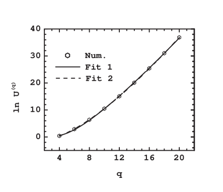
Figure 1: $\ln(U^{(q)\star})$ and the two fits described in the text.

The two fits can barely be distinguished in Fig. 1. If as in Fit 1 we use a general fit of the form

$$U^{(q)\star}\simeq A(q!)^{B}\exp(Cq)\ ,$$ (26)

then the values of the parameters change if we exclude the points with low values of $q$. For instance if we exclude the first five points, $B\simeq 1.15$ instead of 1.29 if we use all the data. The intermediate values are shown on Fig. 2. Using a nonlinear fit to determine how $B$ depends on this choices, we found that $B\simeq 0.99+0.61q^{-0.52}$ where $q$ is the smallest index in the dataset used to obtain $B$. We conclude that the asymptotic value is very close to 1 and that the the leading growth is

$$U^{(q)\star}\approx q!\ ,$$ (27)

This result is similar to what is found in Ref. Goldberg (1990); Cornwall (1990); Zakharov (1991); Voloshin (1992) for other models studied in the context of multiparticle production. Note that the generating function of the connected $2l$-points function has a $1/(2l)!$ factor at order $2l$ (see Eq. (5)) which indicates that the expansion of the generating function of the connected functions in powers of an external field has a finite radius of convergence (see section VII for more discussion).

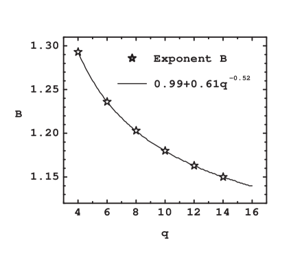
Figure 2: Value of the fitted exponent of the factorial for different sets of data. The abscissa is the smallest value of $q$ used in the data set.

VI Correction to Scaling Amplitudes

Ratios of subleading amplitudes are also expected to be universal Wegner (1976); Aharony and Ahlers (1980); Chang and Houghton (1980). To express these quantities we first define the relative strength of the corrections $a^{(q)}\equiv A_{1}^{(q)}/A_{0}^{(q)}$. From these, we define the ratios

$$S^{(q)\star}=\frac{a^{(q)}}{a^{(2)}}\ .$$

For the measures considered here, we found the approximately universal values shown in Table 2 with uncertainties of order 1 in the last digit. Particular values are given in the Appendix.

Table 2: Universal values of $S^{(2l)\star}$ .

2l	$S^{(2l)\star}$
4	2.03
6	3.26
8	4.52
10	5.8
12	7.1
14	8.3
16	9.6
18	11
20	12

These values can be fitted well with a linear function as shown in Fig. 3

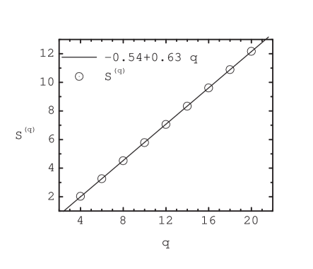
Figure 3: Ratios of subleading amplitudes $S^{(q)}$

VII The effective potential

In this section, we compare our results with related results obtained for models in the same class of universality as the 3 dimensional Ising model with nearest neighbor interactions. In order to avoid repetitions, we follow sections V, VII and Appendix C of Campostrino, Pelissetto, Rossi and Vicari Campostrini et al. (1999) (CPRV for short). We follow exactly their notations except for the fact that we keep using superscripts in $\chi^{(2q)}$ to denote the connected $2q$-points function (denoted $\chi_{2q}$ in CPRV). It should also be mentioned that in the case of Dyson’s model, there is no wave function renormalization and consequently some of the rescalings introduced in CPRV are not necessary in the present case.

In CPRV, a universal function

$$A(z)=z^{2}/2+z^{4}/24+\sum_{l\geq 3}\frac{r_{2l}}{(2l)!}z^{2l}\ ,$$ (28)

obtained from the effective potential by suitable rescalings of the effective potential and its argument (the magnetization) is defined (Eq. (5.7)). The universal coefficients $r_{2l}$ are ratios of amplitudes associated with the 1PI. They can be expressed in terms of the connected Green’s functions by expanding the magnetization as a power series of the magnetic field in the equation defining the Legendre transform. Explicit formulas for $r_{6}$, $r_{8}$ and $r_{10}$ are given in Eqs. (5.23-25) of CPRV. These quantities can be trivially reexpressed section V. For instance,

$$r_{6}=10-\frac{U^{(6)\star}}{(U^{(4)\star})^{2}}\ .$$ (29)

In CPRV, “Griffiths’ s analyticity”is invoked to justify that $A(z)$ in Eq. (28) has a finite radius of convergence. This requires, for large $l$, a growth not faster than

$$r_{2l}\propto(C_{1})^{l}(2l)!\ .$$ (30)

The coefficients of $r_{2l}$ grow rapidly as can be observed in

$$r_{12} = 1401400-560560\frac{\chi^{(2)}\chi^{(6)}}{{\chi^{(4)}}^{2}}+36036\frac{{\chi^{(2)}}^{2}{\chi^{(6)}}^{2}}{{\chi^{(4)}}^{4}}$$ (31)

$$+ 17160\,\frac{{{{\chi}^{(2)}}}^{2}\,{{\chi}^{(8)}}}{{{{\chi}^{(4)}}}^{3}}-792\,\frac{{{{\chi}^{(2)}}}^{3}\,{{\chi}^{(6)}}\,{{\chi}^{(8)}}}{{{{\chi}^{(4)}}}^{5}}$$

$$- 220\,\frac{{{{\chi}^{(2)}}}^{3}\,{{\chi}^{({10})}}}{{{{\chi}^{(4)}}}^{4}}+\frac{{{{\chi}^{(2)}}}^{4}\,{{\chi}^{({12})}}}{{{{\chi}^{(4)}}}^{5}}\ ,$$

and

$$r_{14} = 190590400-95295200\,\frac{{{\chi}^{(2)}}\,{{\chi}^{(6)}}}{{{{\chi}^{(4)}}}^{2}}$$ (32)

$$+ 10090080\,\frac{{{{\chi}^{(2)}}}^{2}\,{{{\chi}^{(6)}}}^{2}}{{{{\chi}^{(4)}}}^{4}}-126126\,\frac{{{{\chi}^{(2)}}}^{3}\,{{{\chi}^{(6)}}}^{3}}{{{{\chi}^{(4)}}}^{6}}$$

$$+ 3203200\,\frac{{{{\chi}^{(2)}}}^{2}\,{{\chi}^{(8)}}}{{{{\chi}^{(4)}}}^{3}}-360360\,\frac{{{{\chi}^{(2)}}}^{3}\,{{\chi}^{(6)}}\,{{\chi}^{(8)}}}{{{{\chi}^{(4)}}}^{5}}$$

$$+ 1716\,\frac{{{{\chi}^{(2)}}}^{4}\,{{{\chi}^{(8)}}}^{2}}{{{{\chi}^{(4)}}}^{6}}-50050\,\frac{{{{\chi}^{(2)}}}^{3}\,{{\chi}^{({10})}}}{{{{\chi}^{(4)}}}^{4}}$$

$$+ 2002\,\frac{{{{\chi}^{(2)}}}^{4}\,{{\chi}^{(6)}}\,{{\chi}^{({10})}}}{{{{\chi}^{(4)}}}^{6}}+364\,\frac{{{{\chi}^{(2)}}}^{4}\,{{\chi}^{({12})}}}{{{{\chi}^{(4)}}}^{5}}$$

$$- \frac{{{{\chi}^{(2)}}}^{5}\,{{\chi}^{({14})}}}{{\chi{(4)}}^{6}}\ .$$

The first (constant) and last (proportional to $\chi^{(2l)}$) terms of the $r_{2l}$ are expected to grow like $(2l)!$. The first term of the $r_{2l}$ (10, 280, 15400, 1401400, etc…) denoted $r^{(0)}_{2l}$, can be obtained from the recursion

$$r_{2l}^{(0)}=\sum_{m=1}^{[2l/3]}r_{2(l-m)}^{(0)}\frac{(-1)^{m+1}}{(2l-3m)!m!6^{m}}\$$ (33)

with the initial conditions $r_{2}^{(0)}=r_{4}^{(0)}=1$. A detailed analysis shows that this leads to a $(2l)!$ growth (with power corrections). On the other hand, we also expect $\chi^{(2l)}\approx(2l)!$ in view of the numerical results of section V. Obviously, if similar rates are found for the intermediate terms, then the bound of Eq. (30) applies.

The numerical values of $r_{6},\dots r_{20}$ for the four measures are given in the Table 8 in the appendix. The results show universality with the same kind of accuracy as in Section V. The universal values are summarized in Table 3.

Table 3: Universal values of $r_{2l}$ calculated numerically and predicted using the CPRV method for the value of $\rho$ given in the last column.

2l	$r_{2l}$	$r_{2l}$ predicted	$\rho$
6	2.0149752	1.81	1.8946
8	2.679529	2.47	1.8946
10	-9.60118	-10.1	1.9218
12	10.7681	8.93	1.9460
14	763.062	753	1.9685
16	-18380.8	$-1.76\times 10^{4}$	2.3197
18	$1.5553\times 10^{6}$	$1.62\times 10^{6}$	2.1889
20	$1.0374\times 10^{7}$	$1.04\times 10^{7}$	2.1181

It should be noted that the numerical values of the $r_{2l}$ are orders of magnitudes smaller than some of the individual terms. For instance, for $r_{14}$, the sum of all the terms $(753)$ is 5 orders of magnitudes smaller than the constant term ($1.9\times 10^{8}$). This requires minute cancellations, and since from the discussion above, some of the terms grow as $(2l)!$, this is a good indication that the bound of Eq. (30) should be satisfied.

We have checked the consistency of our results by using the method proposed by CPRV to predict $r_{2(l+1)}$, using $r_{2},\dots r_{2l}$ as input. As one can see from Table 3, the two results are in reasonable agreement (relative errors of the order of 10 percent). One can also calculate $r_{2(l+2)}$ etc.. from the same input, but the agreement is not as good. It should noted that Eq. (7.21) in CPRV, for the intermediate parameter $\rho$, admits in general more than one positive root. The numbers given here have been obtained by using the smallest positive root also given in Table 3. We also found that the equations leading to the prediction of $r_{6}$ and $r_{8}$ were identical. A detailed analysis shows that it is due to the fact that the magnetization exponent (usually denoted $\beta$) is $\gamma/4$ Godina et al. (2000) for Dyson’s model .

The logarithm of $|r_{2l}|$ is displayed in Fig. 4. The growth looks roughly similar to the growth of the $U^{(2l)\star}$ shown in Fig. 1, however the behavior is not as smooth. It is possible to obtain decent fits of the data of Fig. 4 with the parametric form

$$\ln|r_{q}|\simeq A+B\ln(q!)+qC\ ,$$ (34)

which is compatible with with Eq. (30). However, the lack of smoothness makes the discrimination against other behavior difficult.

Figure 4: Values of $\ln|r_{q}|$ versus $q$

A better way to identify the asymptotic behavior consists in studying the ratios

$$P^{(2l)}\equiv\frac{r_{2l+2}}{r_{2l}}\ .$$ (35)

The factorial rate of Eq. (30) would imply that for $l$ large enough,

$$P^{(2l)}\propto l^{2}\ ,$$ (36)

which means a line of slope 2 in a log-log plot. Such a plot is provided in Fig. 5. The data is quite scattered, however, the overall rate of growth seems compatible with Eq. (36), the slope of the linear fit being 2.36. Note that without the last four data points, one might be tempted to conclude that the ratios are constant (this would imply an exponential growth rather than a factorial one). The same quantity with $r_{2l}$ replaced by $U^{(2l)*}$ is also provided for comparison. In this case, the linear behavior is quite evident and the slope slowly decreases from 2.22 to 2.11 as we remove one by one the first five data points as was done in section V.

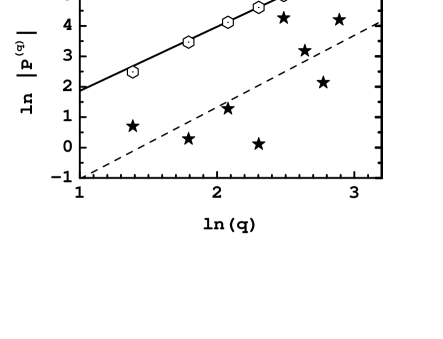
Figure 5: Values of $\ln|P^{(2l)}|$ versus $\ln 2l$. The stars correspond to ratios of $r_{2l}$ as defined in Eq. (35). The hexagons correspond to the same quantity but with $r_{2l}$ replaced by $U^{(2l)*}$. The lines are linear fits, the slope of the solid line is 2.11 while the slope of the dashed line is 2.36.

Our values of $r_{2l}$ are not very different from $r_{6}=2.048(5)$, $r_{8}=2.28(8)$ and $r_{10}=-13(4)$ obtained by CPRV with an improved high-temperature method or the values obtained by other authors with other methods (see Table VIII in CPRV for details). This can be explained from the fact that even though Dyson’s model belongs to a different class of universality, the critical exponents are not very different. This is encouraging for the possibility of improving the hierarchical approximation. Estimates of $r_{12}$ and $r_{14}$ can be obtained from Ref. Morris (1996a). Using the translation $r_{2l}=(2l-1)!F_{2l-1}$, we obtain $r_{12}=38(16)$ with a sharp cutoff LPA and, $r_{12}=20(12)$ and $r_{14}=560(370)$ at lowest order in the derivative expansion. It is also interesting to compare the values $F_{5}=0.01679$, $F_{7}=5.317\times 10^{-4}$ and $F_{9}=-2.646\times 10^{-5}$ obtained with our data with the various entries of Table 7 in Ref. Morris (1997). Again, the values have the same order of magnitude, but no precise correspondence exists with any of the approximations listed.

VIII Conclusions

We have calculated numerically the leading and subleading amplitudes corresponding to 4 randomly chosen local measures for the $2l$-point functions up to $l$ =10. We found good evidence for approximate universal relations which allow, for the model considered here, to predict the amplitudes of all the connected $2l$-point functions in terms of the amplitude for the 2-point function. We found clear indication that the universal amplitudes associated with the connected $2l$-point function grow as $(2l)!$. In the context of perturbation theory, this growth seems to be related to the asymptotic nature of the expansion Goldberg (1990); Cornwall (1990); Zakharov (1991); Voloshin (1992). However, our result is completely nonperturbative and indicates that the expansion of the generating function of the connected functions in power of the external field has a finite radius of convergence (since this generating function, as the universal function $A(z)$ of Eq. (28), has $1/(2l)!$ factors in its definition).

These results can also be used to calculate universal coefficients, denoted $r_{2l}$, appearing in the effective potential and which have been calculated with a variety of methods Tetradis and Wetterich (1994); Tsypin (1994); Guida and Zinn-Justin (1997); Morris (1997); Pelissetto and Vicari (1998); Campostrini et al. (1999, 2000); Pelissetto and Vicari (2002) for the universality class of the 3D Ising model with nearest neighbor interactions. Our results are compatible with universality with at least 5 significant digits. They are of the same order of magnitude as the existing estimates for other models. To the best of our knowledge, we have presented the first numerical estimates of $r_{16}$, $r_{18}$ and $r_{20}$. They are compatible with a factorial growth of the $r_{2l}$ and the expectation that the universal function $A(z)$ has a finite radius of convergence Campostrini et al. (1999).

Our model does not pretend to be realistic. The fact that the non-perturbative continuum limit in this simplified case leads to a situation where we have high predictivity should be seen as an encouragement to look for nontrivial fixed point in more realistic theories. The application of the method to four dimensional models requires further investigation. The common wisdom is that in the pure scalar case, there is no non-trivial fixed point in 4D Wilson and Kogut (1974); Luscher and Weisz (1987) (see however the discussion of Refs. Halpern and Huang (1995, 1996); Morris (1996b)). On the other hand, for 4D models involving fermions and gauge fields, the question is more complex and stretches the limits of our present computational abilities (see for instance the discussion of compact abelian fields coupled to fermions Kogut and Strouthos (2003) or BCS inspired models of top condensation Bardeen et al. (1990)). As the Higgs sector will soon be probed at unexplored energies, a special effort should be made to understand these questions.

*

Appendix A Numerical results for particular measures

In this appendix, we provide numerical results obtained with the measures given in Table 4 and the Ising measure.

Table 4: Measures used for particular calculations.

LG(I)	Exp[-0.5$\phi^{2}$-10$\phi^{4}$]	$\beta_{c}$=7.7036412465997630
LG(II)	Exp[-2$\phi^{2}$-0.2$\phi^{6}$]	$\beta_{c}$=3.1273056619243551
LG(III)	Exp[-0.1$\phi^{2}$-0.4$\phi^{8}$]	$\beta_{c}$=2.2259466376795976

Table 5: $a^{(q)}/a^{(2)}$ Ratios for LG measures

	LG(I)		LG(II)		LG(III)
$q$	$|a^{(q)}|$	$a^{(q)}/a^{(2)}$	$|a^{(q)}|$	$a^{(q)}/a^{(2)}$	$|a^{(q)}|$	$a^{(q)}/a^{(2)}$
2	0.10424	1.00000	0.21404	1.00000	0.31178	1.00000
4	0.21156	2.02961	0.43401	2.02776	0.63339	2.03152
6	0.33980	3.25988	0.69834	3.26266	1.10602	3.25877
8	0.47075	4.51615	0.96793	4.52219	1.04700	4.51281
10	0.60271	5.78214	1.24482	5.81582	1.80103	5.77662
12	0.73514	7.05257	1.51927	7.09805	2.19654	7.04517
14	0.86783	8.32554	1.79472	8.38498	2.59268	8.31573
16	1.00068	9.60004	2.07087	9.67519	2.98897	9.58678
18	1.13361	10.8753	2.34760	10.9681	3.38638	10.8615
20	1.26664	12.1515	2.62528	12.2654	3.78335	12.1347

Table 6: $a^{(q)}/a^{(2)}$ Ratios for the Ising measure

$q$	$a^{(q)}$	$a^{(q)}/a^{(2)}$	$q$	$a^{(q)}$	$a^{(q)}/a^{(2)}$	$q$	$a^{(q)}$	$a^{(q)}/a^{(2)}$
2	0.5614	1.00000	10	3.24785	5.78527	18	6.11352	10.88978
4	1.13943	2.02962	12	3.96229	7.05787	20	6.83208	12.16971
6	1.83040	3.26042	14	4.66892	8.31657
8	2.53632	4.51785	16	5.39558	9.61094

Table 7: Dimensionless couplings $U^{(q)\star}$

$q$	LG(I)	LG(II)	LG(III)	Ising
4	1.5058710	1.5058706	1.5058710	1.5058709
6	18.10722	18.10721	18.10722	18.10722
8	579.9701	579.9698	579.9702	579.9702
10	35653.80	35653.77	35653.80	35653.80
12	3.577694E6	3.577690E6	3.577694E6	3.577694E6
14	5.317628E8	5.317622E8	5.317628E8	5.317627E8
16	1.097204E11	1.097203E11	1.097205E11	1.097204E11
18	3.00025E13	3.00024E13	3.00024E13	3.00025E13
20	1.04998E16	1.04997E16	1.04998E16	1.04997E16

Table 8: $r_{2l}$ values for the four measures considered, their averages and estimated errors.

$2l$	LGI	LGII	LGIII	Ising	Average	Error
6	2.0149752	2.0149751	2.0149752	2.0149752	2.01497516	6$\times 10^{-8}$
8	2.6795292	2.6795279	2.6795295	2.6795289	2.6795289	7$\times 10^{-7}$
10	-9.6011836	-9.6011888	-9.6011824	-9.6011849	9.601185	3$\times 10^{-6}$
12	10.768076	10.768118	10.768070	10.768086	10.76809	0.00002
14	763.06239	763.06185	763.06229	763.06192	763.0621	0.0003
16	-18380.758	-18380.885	-18380.933	-18380.816	-18380.85	0.08
18	155520.69	155541.95	155500.45	155543.79	155526.72	20.42
20	1.0366406E7	1.0378039E7	1.0377558E7	1.0373698E7	1.0374$\times 10^{7}$	5$\times 10^{3}$

References

- Hagiwara et al. (2002) K. Hagiwara et al. (Particle Data Group), Phys. Rev. D66, 010001 (2002).
- K.Wilson (1972) K.Wilson, Phys. Rev. D 6, 419 (1972).
- Godina et al. (1998a) J. Godina, Y. Meurice, and M. Oktay, Phys. Rev. D 57, R6581 (1998a).
- Privman et al. (1991) V. Privman, P. C. Hohenberg, and A. Aharony, in Phase Transitions and Critical Phenonema, Vol. 14, edited by L. Domb and J. Lebowitz (Academic Press, New York, 1991), pp. 4–121.
- Campostrini et al. (1999) M. Campostrini, A. Pelissetto, P. Rossi, and E. Vicari, Phys. Rev. E60, 3526 (1999), eprint cond-mat/9905078.
- Tetradis and Wetterich (1994) N. Tetradis and C. Wetterich, Nucl. Phys. B422, 541 (1994), eprint hep-ph/9308214.
- Guida and Zinn-Justin (1997) R. Guida and J. Zinn-Justin, Nucl. Phys. B489, 626 (1997), eprint hep-th/9610223.
- Morris (1997) T. R. Morris, Nucl. Phys. B495, 477 (1997), eprint hep-th/9612117.
- Pelissetto and Vicari (1998) A. Pelissetto and E. Vicari, Nucl. Phys. B522, 605 (1998), eprint cond-mat/9801098.
- Campostrini et al. (2000) M. Campostrini, A. Pelissetto, P. Rossi, and E. Vicari, Phys. Rev. B62, 5843 (2000), eprint cond-mat/0001440.
- Tsypin (1994) M. M. Tsypin, Phys. Rev. Lett. 73, 2015 (1994).
- Pelissetto and Vicari (2002) A. Pelissetto and E. Vicari, Phys. Rept. 368, 549 (2002), eprint cond-mat/0012164.
- Dyson (1969) F. Dyson, Comm. Math. Phys. 12, 91 (1969).
- Baker (1972) G. Baker, Phys. Rev. B 5, 2622 (1972).
- Meurice (2003) Y. Meurice, Phys. Rev. E (in press) (2003), eprint cond-mat/0312188.
- Parisi (1988) G. Parisi, Statistical Field Theory (Addison Wesley, New York, 1988).
- Goldberg (1990) H. Goldberg, Phys. Lett. B246, 445 (1990).
- Cornwall (1990) J. M. Cornwall, Phys. Lett. B243, 271 (1990).
- Zakharov (1991) V. I. Zakharov, Phys. Rev. Lett. 67, 3650 (1991).
- Voloshin (1992) M. B. Voloshin, Nucl. Phys. B383, 233 (1992).
- Aharony and Ahlers (1980) A. Aharony and G. Ahlers, Phys. Rev. Lett. 44, 782 (1980).
- Chang and Houghton (1980) M. Chang and A. Houghton, Phys. Rev. Lett. 44, 785 (1980).
- Wegner (1976) F. J. Wegner, in Phase Transitions and Critical Phenonema, Vol. 6, edited by L. Domb and M. S. Green (Academic Press, New York, 1976), pp. 7–124.
- Koch and Wittwer (1995) H. Koch and P. Wittwer, Math. Phys. Electr. Jour. 1, Paper 6 (1995).
- Godina et al. (1999) J. Godina, Y. Meurice, and M. Oktay, Phys. Rev. D 59, 096002 (1999).
- Godina et al. (1998b) J. Godina, Y. Meurice, M. Oktay, and S. Niermann, Phys. Rev. D 57, 6326 (1998b).
- Wilson (1971) K. Wilson, Phys. Rev. B. 4, 3185 (1971).
- Meurice and Ordaz (1996) Y. Meurice and G. Ordaz, J. Phys. A (Letter to the Editor) 29, L635 (1996).
- Godina et al. (2000) J. J. Godina, Y. Meurice, and M. Oktay, Phys. Rev. D 61, 114509 (2000).
- Niemeijer and van Leeuwen (1976) T. Niemeijer and J. van Leeuwen, in Phase Transitions and Critical Phenomena, vol. 6, edited by C. Domb and M. Green (Academic Press, New York, 1976).
- Meurice et al. (1995) Y. Meurice, G. Ordaz, and V. G. J. Rodgers, Phys. Rev. Lett. 75, 4555 (1995).
- Meurice et al. (1997) Y. Meurice, S. Niermann, and G. Ordaz, J. Stat. Phys. 87, 363 (1997).
- (33) M. B. Oktay, Nonperturbative methods for hierarchical models, (Ph. D. thesis), UMI-30-18602.
- Glazek and Wilson (2002) S. D. Glazek and K. G. Wilson, Phys. Rev. Lett. 89, 230401 (2002), eprint hep-th/0203088.
- Braaten and Hammer (2003) E. Braaten and H. W. Hammer, Phys. Rev. Lett. 91, 102002 (2003), eprint nucl-th/0303038.
- Glimm and Jaffe (1987) J. Glimm and A. Jaffe, Quantum Physics (Springer-Verlag, New York, 1987).
- Morris (1996a) T. R. Morris, Nucl. Phys. B458, 477 (1996a), eprint hep-th/9508017.
- Wilson and Kogut (1974) K. Wilson and J. Kogut, Phys. Rep. 12, 75 (1974).
- Luscher and Weisz (1987) M. Luscher and P. Weisz, Nucl. Phys. B290, 25 (1987).
- Halpern and Huang (1995) K. Halpern and K. Huang, Phys. Rev. Lett. 74, 3526 (1995), eprint hep-th/9406199.
- Halpern and Huang (1996) K. Halpern and K. Huang, Phys. Rev. Lett. 77, 1659 (1996).
- Morris (1996b) T. R. Morris, Phys. Rev. Lett. 77, 1658 (1996b), eprint hep-th/9601128.
- Kogut and Strouthos (2003) J. B. Kogut and C. G. Strouthos, Phys. Rev. D67, 034504 (2003), eprint hep-lat/0211024.
- Bardeen et al. (1990) W. A. Bardeen, C. T. Hill, and M. Lindner, Phys. Rev. D41, 1647 (1990).