hep-th/0401139

Boundary RG Flows of N=2 Minimal Models
Kentaro Hori

University of Toronto, Toronto, Ontario, Canada

We study boundary renormalization group flows of ${\mathcal{N}}=2$ minimal models using Landau-Ginzburg description of B-type. A simple algebraic relation of matrices is relevant. We determine the pattern of the flows and identify the operators that generate them. As an application, we show that the charge lattice of B-branes in the level $k$ minimal model is ${\mathbb{Z}}_{k+2}$. We also reproduce the fact that the charge lattice for the A-branes is ${\mathbb{Z}}^{k+1}$, applying the B-brane analysis on the mirror LG orbifold.

1 Introduction

Many systems in statistical mechanics and quantum field theory have effective description of Landau-Ginzburg (LG) type. In particular, in $(2,2)$ supersymmetric field theories in $1+1$ dimensions, LG models provide effective description of a large class of theories, both conformal and massive, from which one can extract intuitive pictures as well as exact results, such as the set and character of vacua, dimension of operators and chiral rings. The simplest example is the single variable model with superpotential

$$W=X^{k+2}$$ (1.1)

labeled by a positive integer $k$. It flows in the infra-red limit to the ${\mathcal{N}}=2$ minimal model at level $k$ — a $(2,2)$ superconformal field theory with central charge $c={3k\over k+2}$ [2, 3, 4, 5, 6], as argued in [7, 8, 9]. LG description gives us a clear picture of renormalization group (RG) flows between conformal field theories. The system with superpotential (1.1) has left and right $U(1)$ R-symmetries which become a part of the superconformal algebra. A vector $U(1)$ is lost if we add a lower order term

$$W=X^{k+2}+\varepsilon X^{\ell}.$$ (1.2)

This can be regarded as a supersymmetric perturbation of the minimal model by a relevant operator, and one can immediately tell by looking at the superpotential that it flows to the model of lower level $\ell-2$.

In this paper, we study the boundary RG flows of Landau-Ginzburg models with an unbroken ${\mathcal{N}}=2$ supersymmetry. Boundary RG flows are being studied from two view points — statistical mechanics of two-dimensional critical systems and string theory. In the latter, boundary RG flows describe, from the worldsheet perspective, the tachyon condensation on the worldvolume of unstable D-brane systems [10]. The subject of unstable D-brane systems [11] has proved to be extremely rich: it motivated the development of string field theory [12, 13], led to the K-theory characterization of D-brane charge [14] and its refinement [15], gave us a physical interpretation of the matrix models [16], and provided workable models of time dependent string theory [17]. In most of them, an important role is played by Chan-Paton factors which are simple matrix factors that live on the worldsheet boundary.

A useful LG description of boundary RG flow already exists. This is in the context of A-branes which are wrapped on Lagrangian submanifolds and support flat gauge fields. In the minimal model and its deformations, the branes are D1-branes at the wedge-shaped lines that reside in the pre-image of $W\in{\mathbb{R}}$ [18]. (The coset construction provides a similar and sometimes useful picture where the branes are straight segment in a disc stretched between special points on the boundary circle [19].) This LG description provides a useful and geometrical picture of RR-charge, Witten index, as well as the appearance of Verlinde algebra [18]. In this description, the boundary RG flow is simply the annihilation of the brane and antibrane (see Figure 1),

Figure 1: Flow of A-type boundary conditions in the minimal model

or recombination of the branes at the intersection points. One can find the pattern of RG flows at a glance. This has been remarked, for example, in [20] (and also in the disc picture in [19, 21]). However, it is not easy to identify the operator that generates a given flow.

There are other class of branes, B-branes, which are wrapped on complex submanifolds and support holomorphic bundles. The purpose of this work is to find a useful picture of boundary RG flows using B-branes in Landau-Ginzburg models, hopefully to the same extent as the A-branes or even to complement what is missing in the A-type picture. B-branes in LG models have been studied in [22, 23, 24, 25, 26, 27, 28]. In particular, we use the recent description by Kontsevich [25, 26, 27, 28] (an independent and alternative description is in [24]) that uses the factorization of the superpotential on the Chan-Paton factor. What is relevant here, it turns out, is the continuous deformation of the matrices

$$M_{t}=\left(\begin{array}[]{cc}A&0\\ 0&1\end{array}\right)\left(\begin{array}[]{cc}\cos t&-\sin t\\ \sin t&\cos t\end{array}\right)\left(\begin{array}[]{cc}1&0\\ 0&B\end{array}\right)\left(\begin{array}[]{cc}\cos t&\sin t\\ -\sin t&\cos t\end{array}\right)$$

that yields the flow

$$\left(\begin{array}[]{cc}A&0\\ 0&B\end{array}\right)\,\mbox{\LARGE$\Rightarrow$}\,\left(\begin{array}[]{cc}AB&0\\ 0&1\end{array}\right).$$ (1.3)

This simple algebraic relation provides the B-type counterpart of the A-type flow as in Figure 1. Also, by a basis change, $M_{t}\rightarrow M_{t}{\cos t\,\,-\sin t\choose\sin t\,\,\,\,\cos t}$, the matrix for small $t$ can be written as

$$M_{\varepsilon}\cong\left(\begin{array}[]{cc}A&0\\ 0&B\end{array}\right)+\varepsilon\left(\begin{array}[]{cc}0&-AB\\ 1&0\end{array}\right).$$ (1.4)

This leads to the boundary analog of (1.2) where the perturbing term breaks the $U(1)$ R-symmetry and generates a flow of the boundary condition. In this way, one can identify the operator that generates a given flow, as well as identify the IR limit of a given perturbation.

As an application, we determine the charge lattice of the D-branes in the minimal model. For B-branes, it turns out that the lattice is torsion

$$\Lambda_{B}\,\cong\,{\mathbb{Z}}_{k+2}.$$

This is obtained through the relation (1.3) or more explicitly

$$\left(\begin{array}[]{cccc}x&&&\\ &\ddots&&\\ &&\ddots&\\ &&&x\end{array}\right)\,\mbox{\LARGE$\Rightarrow$}\,\left(\begin{array}[]{cccc}x^{k+2}&&&\\ &1&&\\ &&\ddots&\\ &&&1\end{array}\right).$$

We also reproduce the charge lattice of A-branes which has been known by the (A-type) LG picture as

$$\Lambda_{A}\,\cong\,{\mathbb{Z}}^{k+1}.$$

This is done by using the mirror symmetry between the minimal model and its ${\mathbb{Z}}_{k+2}$-orbifold, where A and B are exchanged, and applying (1.3) to the latter.

Note: While this work is being written, we noticed a paper [30] which studies boundary RG flows of non-supersymmetric minimal models in LG description. Also, a paper [31] just appeared which has some overlaps in the discussion of B-branes in LG orbifolds.

2 B-branes in Landau-Ginzburg Models

Let $X$ be a non-compact Calabi-Yau manifold with a (local) Kähler potential $K(\phi,\overline{\phi})$ and a global holomorphic function $W(\phi)$. We consider the $(2,2)$ supersymmetric LG model with the action

$$S=S_{K}+S_{W}=\int_{\Sigma}{\rm d}^{2}x\left[\,\int{\rm d}^{4}\theta\,K(\Phi,\overline{\Phi})\,+{\rm Re}\int{\rm d}^{2}\theta\,W(\Phi)\,\right].$$ (2.1)

For superspace and superfields we use the convention of [23]. We are interested in B-branes of this system. Namely, the boundary conditions and interactions preserving the B-type ${\mathcal{N}}=2$ supersymmetry $Q=Q_{+}+Q_{-}$, $\overline{Q}=\overline{Q}_{+}+\overline{Q}_{-}$ [32].

Under the transformation $\delta=\epsilon Q-\overline{\epsilon}\overline{Q}$, the Kähler potential term (D-term) $S_{K}$ is invariant with the ordinary supersymmetric boundary condition for D-branes wrapped on a complex submanifold of $X$. On the other hand, the superpotential term (F-term) varies as [34, 22]

$$\delta S_{W}={\rm Re}\int_{\partial\Sigma,B}{\rm d}t\,{\rm d}\theta(-i\overline{\epsilon})\,W(\Phi)\,,$$ (2.2)

where $\int_{\partial\Sigma,B}$ is the integration on the B-boundary in which $\theta^{+}=\theta^{-}=:\theta$ (see [22] for conventions on “boundary superspace”). This vanishes if the D-brane lies in a level set of the superpotential $W$ [33, 18]. There is actually an alternative way to preserve the B-type supersymmetry [35]. Suppose the superpotential can be written as the product

$$W(\Phi)=if(\Phi)g(\Phi).$$ (2.3)

Then, we add a boundary term

$$S_{\rm bdry}=\int_{\partial\Sigma}{\rm d}t\,\left[\,{1\over 2}\int_{B}{\rm d}\theta{\rm d}\overline{\theta}\,\overline{\Gamma}\Gamma\,+\,{\rm Re}\int_{B}{\rm d}\theta\,\Gamma f(\Phi)\,\right].$$ (2.4)

where $\Gamma$ is a fermionic superfield on the B-boundary which fails to be chiral,

$$\overline{D}\Gamma=g(\Phi).$$ (2.5)

Under the B-type supersymmetry the boundary term varies as

$$\delta S_{\rm bdry} = {\rm Re}\int_{\partial\Sigma,B}{\rm d}t{\rm d}\theta\,\left(\left[\epsilon{\mathcal{Q}}-\overline{\epsilon}\overline{\mathcal{Q}}\right]\Gamma f(\Phi)\right)\Bigl{|}_{\overline{\theta}=0}$$

$$= {\rm Re}\int_{\partial\Sigma,B}{\rm d}t{\rm d}\theta\,(-\overline{\epsilon}\overline{D}\Gamma f(\Phi))\Bigl{|}_{\overline{\theta}=0}={\rm Re}\int_{\partial\Sigma,B}{\rm d}t{\rm d}\theta\,i\overline{\epsilon}W(\Phi)\,,$$

which indeed cancels $\delta S_{W}$. Thus we find a B-brane for each factorization of the superpotential (2.3). More generally, if the superpotential is expressed as $W=i\sum_{\alpha=1}^{r}a_{\alpha}b_{\alpha}$, one can do the same by introducing $\Gamma_{\alpha}$ obeying $\overline{D}\Gamma_{\alpha}=b_{\alpha}(\Phi)$ with the boundary superpotential $\sum_{\alpha=1}^{r}\Gamma_{\alpha}a_{\alpha}(\Phi)$. It is straightforward to generalize this to the case of gauged linear or non-linear sigma models with superpotential.

The component expression of a superfield with constraint $\overline{D}\Gamma=g(\Phi)$ is $\Gamma=\eta+\theta G-i\theta\overline{\theta}\dot{\eta}-\overline{\theta}g(\Phi)$ and the boundary term reads as

$$S_{\rm bdry} = \int_{\partial\Sigma}{\rm d}t\left\{i\overline{\eta}\dot{\eta}-{1\over 2}|g(\phi)|^{2}-{\rm Re}\Bigl{(}\overline{\eta}\partial_{i}g(\phi)\psi^{i}\Bigr{)}+{1\over 2}|G|^{2}+{\rm Re}\Bigl{(}-\eta\partial_{i}f(\phi)\psi^{i}+Gf(\phi)\Bigr{)}\right\}$$

$$= \int_{\partial\Sigma}{\rm d}t\left\{i\overline{\eta}\dot{\eta}-{1\over 2}|g(\phi)|^{2}-{1\over 2}|f(\phi)|^{2}-{\rm Re}\Bigl{(}\overline{\eta}\partial_{i}g(\phi)\psi^{i}+\eta\partial_{i}f(\phi)\psi^{i}\Bigr{)}\right\}$$

where $\psi^{i}:=\psi^{i}_{+}+\psi^{i}_{-}$. The auxiliary field $G$ is eliminated by solving $G=-\overline{f(\phi)}$. The supersymmetry variation of the fermion $\eta$ is $\delta\eta=\epsilon G-\overline{\epsilon}g(\phi)=-\epsilon\overline{f(\phi)}-\overline{\epsilon}g(\phi)$. Let us formulate the system on the segment $0\leq\sigma\leq\pi$ where we put the fermions $\eta_{0}$ and $\eta_{\pi}$ at the two boundaries with the boundary terms corresponding to the factorizations

$$W=if_{0}g_{0}=if_{\pi}g_{\pi}.$$

The boundary at $\sigma=0$ is oriented toward the past $t\rightarrow-\infty$ while the $\sigma=\pi$ boundary is oriented toward the future $t\rightarrow+\infty$. By Nöther procedure we find the supercharge $Q=Q_{\rm bulk}+Q_{\rm bdry}$, $\overline{Q}=\overline{Q}_{\rm bulk}+\overline{Q}_{\rm bdry}$ where

$$\overline{Q}_{\rm bulk}=\int_{0}^{\pi}{\rm d}\sigma\Bigl{\{}(\overline{\psi}_{+}+\overline{\psi}_{-})\cdot\partial_{t}\phi+(\overline{\psi}_{+}-\overline{\psi}_{-})\cdot\partial_{\sigma}\phi+i(\psi_{-}-\psi_{+})^{i}\partial_{i}W(\phi)\Bigr{\}}$$

$$\overline{Q}_{\rm bdry}=-i\Bigl{[}\,\eta f(\phi)\,+\,\overline{\eta}g(\phi)\,\Bigr{]}^{\pi}_{0}.$$

Using the canonical (anti)commutation relation, we find

$$\overline{Q}_{\rm bulk}^{2}=-iW\Bigl{|}_{0}^{\pi},\quad\{\overline{Q}_{\rm bulk},\overline{Q}_{\rm bdry}\}=0,\quad\overline{Q}_{\rm bdry}^{2}=iW\Bigl{|}_{0}^{\pi},$$ (2.6)

and indeed the total supercharge $\overline{Q}$ is nilpotent. The fermion at $\sigma=\pi$ is represented on a two dimensional vector space ${\mathbb{C}}^{2}_{\pi}$ spanned by $|0\rangle_{\pi},\overline{\eta_{\pi}}|0\rangle_{\pi}$. This is the Chan-Paton factor of the brane. The Chan-Paton factor for the brane at $\sigma=0$ is likewise ${\mathbb{C}}^{2}_{0}$ spanned by $|0\rangle_{0},\overline{\eta_{0}}|0\rangle_{0}$. Both spaces are ${\mathbb{Z}}_{2}$ graded by the fermion number — $|0\rangle$ is bosonic and $\overline{\eta}|0\rangle$ is fermionic. Open string states take values in ${\rm Hom}({\mathbb{C}}_{0}^{2},{\mathbb{C}}_{\pi}^{2})$ on which the boundary part of the supercharge is represented as

$$i\overline{Q}_{\rm bdry}\left(\begin{array}[]{cc}a&b\\ c&d\end{array}\right)=\left(\begin{array}[]{cc}0&f_{\pi}(\phi)\\ g_{\pi}(\phi)&0\end{array}\right)\left(\begin{array}[]{cc}a&b\\ c&d\end{array}\right)-\left(\begin{array}[]{cc}a&-b\\ -c&d\end{array}\right)\left(\begin{array}[]{cc}0&f_{0}(\phi)\\ g_{0}(\phi)&0\end{array}\right).\\$$

Since $X$ is assumed to be Calabi-Yau, the supersymmetric ground states are determined by the zero mode analysis. The zero mode Hilbert space is represented as the space of ${\rm Hom}({\mathbb{C}}^{2}_{0},{\mathbb{C}}^{2}_{\pi})$-valued antiholomorphic forms on $X$ on which the supercharge acts as the Dolbeault operator plus (2):

$$i\overline{Q}=\overline{\partial}+i\overline{Q}_{\rm bdry}$$

(In the zero mode sector, the left and the right boundaries are mapped to the same point and thus $\overline{Q}_{\rm bulk}^{2}=\overline{Q}_{\rm bdry}^{2}=0$.) Note that this forms a ${\mathbb{Z}}_{2}$-graded complex where the grading comes from the mod 2 reduction of form degree and the fermion number in ${\rm Hom}({\mathbb{C}}^{2}_{0},{\mathbb{C}}^{2}_{\pi})$. The space of supersymmetric ground states can be identified as the $\overline{Q}$-cohomology group. If $X$ is a Stein space, this reduces to the cohomology of $\overline{Q}_{\rm bdry}$ acting on the space of ${\rm Hom}({\mathbb{C}}^{2}_{0},{\mathbb{C}}^{2}_{\pi})$-valued holomorphic functions on $X$:

$${\mathcal{H}}_{\rm SUSY}\cong H(\Gamma_{\it hol}(X,{\rm Hom}({\mathbb{C}}^{2}_{0},{\mathbb{C}}^{2}_{\pi}));\overline{Q}_{\rm bdry}).$$ (2.7)

If the brane corresponds to more general “factorization”, $W=i\sum_{\alpha=1}^{r}a_{\alpha}b_{\alpha}$, the Chan-Paton factor is ${\mathbb{C}}^{2^{r}}$ spanned by the exterior powers of $\overline{\eta}_{\alpha}$ multiplied to the state $|0\rangle$ annihilated by $\eta_{\alpha}$. The operator $i\overline{Q}_{\rm bdry}$ acts as $\sum_{\alpha=1}^{r}(\eta_{\alpha}a_{\alpha}+\overline{\eta}_{\alpha}b_{\alpha})$, exchanging the bosonic and fermionic subspaces of ${\mathbb{C}}^{2^{r}}$. Let $f$ (resp. $g$) be the restriction of this operator on the fermionic (resp. bosonic) subspace. Then, $fg$ and $gf$ are both proportional to $-iW$. One can further generalize the Chan-Paton factor to an arbitrary ${\mathbb{Z}}_{2}$-graded vector space $V=V_{+}\oplus V_{-}$ on which there are operators $g:V_{+}\rightarrow V_{-}$ and $f:V_{-}\rightarrow V_{+}$ such that

$$fg=-iW{\bf 1}_{V_{+}},\qquad gf=-iW{\bf 1}_{V_{-}}.$$ (2.8)

The boundary action is given by the super-Wilson-line for the superconnection

$${\mathcal{A}}={1\over 2}\left(\begin{array}[]{cc}ff^{{\dagger}}+g^{{\dagger}}g&\psi^{i}\partial_{i}f+\overline{\psi}^{\overline{\imath}}\partial_{\overline{\imath}}g^{{\dagger}}\\ \psi^{i}\partial_{i}g+\overline{\psi}^{\overline{\imath}}\partial_{\overline{\imath}}f^{{\dagger}}&f^{{\dagger}}f+gg^{{\dagger}}\end{array}\right).$$

This is the same as the standard super-Wilson-line factor for the brane-antibrane system [36, 37] corresponding to the tachyon field $T=f+g^{{\dagger}}:V_{-}\rightarrow V_{+}$ (up to the shift by ${\rm Im}(W)$). Let $(V_{-}\mathop{\rightleftharpoons}^{\!\!\!\!\!\!f}_{\!\!\!\!\!\!g}V_{+})_{0}$ and $(V_{-}\mathop{\rightleftharpoons}^{\!\!\!\!\!\!f}_{\!\!\!\!\!\!g}V_{+})_{\pi}$ be two such branes and consider the open string stretched between them. The space of supersymmetric ground states is isomorphic to the cohomology group

$${\mathcal{H}}_{\rm SUSY}\cong H(\Gamma_{\it hol}(X,{\rm Hom}(V_{0},V_{\pi}));\overline{Q}_{\rm bdry}),$$ (2.9)

where $\overline{Q}_{\rm bdry}$ is defined as in (2).

This realization of the space of supersymmetric ground states was obtained by Kontsevich whose work is interpreted in the above form in [25]. An independent work on the same subject is done by the author [22, 23, 24]. In [24] a different form of the cohomological realization is obtained (see also [23] for a preliminary version which gives the derivation). We also note that some mathematical predictions of these results combined with Mirror Symmetry [38] were confirmed in [39, 40].

3 B-Branes in ${\mathcal{N}}=2$ Minimal Models

Let us consider the Landau-Ginzburg model of a single variable $X$ with the Kähler potential $K=|X|^{2}$ and superpotential

$$W=iX^{k+2}.$$

Since the superpotential is homogeneous, this model has a vector R-symmetry $U(1)_{V}:X(\theta^{\pm})\rightarrow\,{\rm e}^{2i\alpha\over k+2}X(\,{\rm e}^{-i\alpha}\theta^{\pm})$, in addition to the axial R-symmetry $U(1)_{A}:X(\theta^{\pm})\rightarrow X(\,{\rm e}^{\mp i\beta}\theta^{\pm})$. There is also a discrete ${\mathbb{Z}}_{k+2}$ symmetry generated by

$$\qquad\quad\gamma:X\rightarrow\omega X,\qquad\omega:=\,{\rm e}^{2\pi i\over k+2}.$$ (3.1)

The system flows in the infra-red limit to a $(2,2)$ sueprconformal field theory of central charge $c={3k\over k+2}$, called the ${\mathcal{N}}=2$ minimal model of level $k$. The two R-symmetries of the LG model define the $U(1)$ currents of the $(2,2)$ superconformal algebra.

3.1 The B-branes $\Scr{B}_{L}$

Let us apply the result of the previous section to this Landau-Ginzburg model. The superpotential can be factorized as $W=ix^{L+1}\cdot x^{k+1-L}$. Thus, for each $L=-1,0,...,k,k+1$, we find a B-brane $\Scr{B}_{L}$ given by the boundary action

$$\int_{\partial\Sigma}{\rm d}t\left[{1\over 2}\int_{B}{\rm d}\theta{\rm d}\overline{\theta}\,\overline{\Gamma}\Gamma\,+\,{\rm Re}\int_{B}{\rm d}\theta\,\Gamma X^{L+1}\right]$$

where $\Gamma$ obeys the constraint $\overline{D}\Gamma=X^{k+1-L}$. The boundary term is invariant under the ${\mathbb{Z}}_{k+2}$ discrete symmetry if we let $\gamma$ acts on the superfield $\Gamma$ by

$$\gamma:\Gamma\rightarrow\omega^{-L-1}\Gamma.$$ (3.2)

Also the vector R-symmetry is preserved under the transformation

$$U(1)_{V}:\Gamma(\theta)\rightarrow\,{\rm e}^{i{k-2L\over k+2}\alpha}\Gamma(\,{\rm e}^{-i\alpha}\theta).$$ (3.3)

If the brane $\Scr{B}_{L}$ defines a conformal boundary condition in the IR limit, we expect that $U(1)_{V}$ becomes a part of the ${\mathcal{N}}=2$ superconformal algebra.

3.2 Supersymmetric Ground States

Let us find the supersymmetric ground states of the open strings. We first consider the string with the both ends at $\Scr{B}_{L}$. Using (2), we find

$$i\overline{Q}_{\rm bdry}\left(\begin{array}[]{cc}a(x)&b(x)\\ c(x)&d(x)\end{array}\right)=\left(\begin{array}[]{cc}x^{L+1}c(x)+b(x)x^{k+1-L}&x^{L+1}(d(x)-a(x))\\ x^{k+1-L}(a(x)-d(x))&x^{k+1-L}b(x)+c(x)x^{L+1}\end{array}\right)$$

It vanishes if and only if $a(x)=d(x)$ and $x^{k+1-L}b(x)+c(x)x^{L+1}=0$. Then, it is $\overline{Q}_{\rm bdry}$-exact when $a(x)$ is divisible by $x^{L+1}$ or $x^{k+1-L}$, $b(x)$ is divisible by $x^{L+1}$ and $c(x)$ is divisible by $x^{k+1-L}$. If $L=-1$ or $L=k+1$, any $\overline{Q}_{\rm bdry}$-closed state is $\overline{Q}_{\rm bdry}$-exact and thus there is no supersymmetric ground state. For $0\leq L\leq k$, there are non-zero $\overline{Q}_{\rm bdry}$-cohomology classes represented by

$$|j\rangle^{b}_{LL}=\left(\begin{array}[]{cc}x^{j}&0\\ 0&x^{j}\end{array}\right),\quad|j\rangle^{f}_{LL}=\left(\begin{array}[]{cc}0&x^{L-j}\\ -x^{k-L-j}&0\end{array}\right);\qquad j=0,1,...,\min\{L,k-L\}.$$ (3.4)

Similarly, for the string stretched from $\Scr{B}_{L_{1}}$ to $\Scr{B}_{L_{2}}$, the $\overline{Q}_{\rm bdry}$-cohomology group is non-trivial for $0\leq L_{1},L_{2}\leq k$ and the basis are represented by

$$|j\rangle^{b}_{L_{1}L_{2}}=\left(\begin{array}[]{cc}\!x^{j-{L_{1}-L_{2}\over 2}}\!&0\\ 0&\!x^{j+{L_{1}-L_{2}\over 2}}\!\end{array}\right),\quad|j\rangle^{f}_{L_{1}L_{2}}=\left(\begin{array}[]{cc}0&\!x^{{L_{1}+L_{2}\over 2}-j}\!\\ \!\!-x^{k-{L_{1}+L_{2}\over 2}-j}\!&0\end{array}\right);\quad$$ (3.9)

$$\qquad\qquad\qquad\mbox{$j={|L_{1}-L_{2}|\over 2},{|L_{1}-L_{2}|\over 2}+1,...,\min\Bigl{\{}{L_{1}+L_{2}\over 2},k-{L_{1}+L_{2}\over 2}\Bigr{\}}$}.$$ (3.10)

In all cases, there are equal number of bosonic and fermionic supersymmetric ground states. This in particular means that the Witten index vanishes

$${\rm Tr}\!\!\mathop{}_{\Scr{B}_{L_{1}}\Scr{B}_{L_{2}}}(-1)^{F}=0.$$ (3.11)

${\mathbb{Z}}_{k+2}$ action

The ${\mathbb{Z}}_{k+2}$ symmetry $X\rightarrow\omega X$, acts on the boundary fermion for the brane $\Scr{B}_{L}$ as $\eta\rightarrow\omega^{-L-1}\eta$ according to (3.2). The action on the Chan-Paton factor is determined by the action on the ground state $|0\rangle_{L}$, which depends on a choice

$$\rho_{M}(\gamma):|0\rangle_{L}\rightarrow\omega^{-{M+L+1\over 2}}|0\rangle_{L}$$ (3.12)

parametrized by a mod $2(k+2)$ integer $M$ such that $L+M+1$ is even. The action on the ground states for the open string stretched from $(\Scr{B}_{L_{1}},\rho_{M_{1}})$ to $(\Scr{B}_{L_{2}},\rho_{M_{2}})$ is

$$\gamma:|j\rangle_{L_{1}L_{2}}^{b}\mapsto\omega^{j+{M_{1}-M_{2}\over 2}}|j\rangle_{L_{1}L_{2}}^{b},\quad|j\rangle_{L_{1}L_{2}}^{f}\mapsto\omega^{-j-1+{M_{1}-M_{2}\over 2}}|j\rangle_{L_{1}L_{2}}^{f}.$$ (3.13)

The open string Witten index twisted by the symmetry $\gamma^{m}$ is given by

$${\rm Tr}\!\!\mathop{}_{(\Scr{B}_{L_{1}},\rho_{M_{1}})(\Scr{B}_{L_{2}},\rho_{M_{2}})}(-1)^{F}\gamma^{m}=\omega^{m{M_{1}-M_{2}\over 2}}\sum_{j\in(\ref{jrange})}\Bigl{(}\omega^{mj}-\omega^{-m(j+1)}\Bigr{)}.$$ (3.14)

R-charges

Let us next analyze the R-charges of these supersymmetric ground states. By (3.3), the R-symmetry acts on the boundary fermion for the brane $\Scr{B}_{L}$ as $\eta\rightarrow\lambda^{k-2L}\eta$ where $\lambda=\,{\rm e}^{i\alpha\over k+2}$. We let the Chan-Paton state $|0\rangle_{L}$ to transform as $|0\rangle_{L}\rightarrow\lambda^{{k\over 2}-L}|0\rangle_{L}$ so that the two states $|0\rangle_{L}$ and $\overline{\eta}|0\rangle_{L}$ have the opposite charges. This yields the following R-transformation of the $L_{1}$-$L_{2}$ open string states:

$$U(1)_{V}:\left(\begin{array}[]{cc}a(x)&b(x)\\ c(x)&d(x)\end{array}\right)\longrightarrow\lambda^{\bullet}\left(\begin{array}[]{cc}\lambda^{-L_{2}+L_{1}}a(\lambda^{2}x)&\lambda^{-L_{2}+k-L_{1}}b(\lambda^{2}x)\\ \lambda^{L_{2}-k+L_{1}}c(\lambda^{2}x)&\lambda^{L_{2}-L_{1}}d(\lambda^{2}x)\end{array}\right)$$

where $\lambda^{\bullet}$ is the factor to be determined. The ground states transform as $|j\rangle_{L_{1}L_{2}}^{b}\mapsto\lambda^{2j+\bullet}|j\rangle_{L_{1}L_{2}}^{b}$ and $|j\rangle_{L_{1}L_{2}}^{f}\mapsto\lambda^{k-2j+\bullet}|j\rangle_{L_{1}L_{2}}^{f}$. We now require that the charge spectrum to be symmetric under the sign flip $q\rightarrow-q$. This fixes $\lambda^{\bullet}$ to be $\lambda^{-{k\over 2}}$. Then, we find that the R-charges of $|j\rangle_{L_{1}L_{2}}^{b}$ and $|j\rangle_{L_{1}L_{2}}^{f}$ are

$$q_{|j\rangle^{b}_{L_{1}L_{2}}}=-q_{|j\rangle^{f}_{L_{1}L_{2}}}={2j\over k+2}-{k\over 2(k+2)}.$$ (3.15)

3.3 Boundary Chiral Primaries

Just as for closed string, there is a one-to-one correspondence with the open string supersymmetric ground states and the boundary chiral ring elements:

$$\Scr{O}^{b}_{j,L_{1}L_{2}}\longleftrightarrow|j\rangle_{L_{1}L_{2}}^{b},\qquad\Scr{O}^{f}_{j,L_{1}L_{2}}\longleftrightarrow|j\rangle_{L_{1}L_{2}}^{f},$$ (3.16)

Their R-charges are obtained from (3.15) by the spectral flow $q\rightarrow q+{c\over 6}$:

$$q_{\Scr{O}^{b}_{j,L_{1}L_{2}}}={2j\over k+2},\qquad q_{\Scr{O}^{f}_{j,L_{1}L_{2}}}={k-2j\over k+2}$$ (3.17)

Under the assumption that $\Scr{B}_{L}$ define conformal boundary conditions, the boundary chiral ring elements define boundary chiral primary fields of the boundary CFT. As usual [41], the R-charge $q$ determines the conformal dimension of the operator $h={q\over 2}$. Thus, the operators $\Scr{O}^{b,f}_{j,L_{1}L_{2}}$ have dimension $h_{j,L_{1}L_{2}}^{b}={j\over k+2}$ and $h_{j,L_{1}L_{2}}^{f}={{k\over 2}-j\over k+2}$.

For the boundary preserving operators, $L_{1}=L_{2}=L$, they can be expressed in terms of the elementary fields as

$$\Scr{O}^{b}_{j,LL}=x^{j},\qquad\Scr{O}^{f}_{j,LL}=\eta x^{L-j}-\overline{\eta}x^{k-L-j}.$$ (3.18)

They indeed represent the non-trivial cohomology classes of $\overline{\delta}x=0,\overline{\delta}\eta=-\overline{\epsilon}x^{k+1-L}$ and $\overline{\delta}\overline{\eta}=-\overline{\epsilon}x^{L+1}$, and have the right R-charge (3.17) under $x\rightarrow\,{\rm e}^{2i\alpha\over k+2}x$, $\eta\rightarrow\,{\rm e}^{{k-2L\over k+2}i\alpha}\eta$, $\overline{\eta}\rightarrow\,{\rm e}^{-{k-2L\over k+2}i\alpha}\overline{\eta}$. The fermionic operator $\Scr{O}_{j,LL}^{f}$ is the lowest component of the superfield $\Gamma X^{L-j}-\overline{\Gamma}X^{k-L-j}$ which is indeed chiral since $\overline{D}\Gamma=X^{k+1-L}$ and $\overline{D}\overline{\Gamma}=X^{L+1}$ (on shell). Thus, the corresponding deformation is given by the boundary F-term

$${\mit\Delta}S_{\rm bdry}={\rm Re}\int_{\partial\Sigma,B}{\rm d}t{\rm d}\theta\,\Bigl{(}\Gamma X^{L-j}-\overline{\Gamma}X^{k-L-j}\Bigr{)}$$

The $t$ integrand is an operator of dimension

$${{k\over 2}-j\over k+2}+{1\over 2}={k+1-j\over k+2}<1,$$

and therefore is relevant.

3.4 The branes $\Scr{B}_{-1}$ and $\Scr{B}_{k+1}$

The branes $\Scr{B}_{-1}$ and $\Scr{B}_{k+1}$ are special in the sense that there is no supersymmetric ground state on the open strings stretched between themselves as well as between them and any other brane. Also, either $f$ or $g$ of the factorization of $W$ is 1 (identity) and the term $|f|^{2}+|g|^{2}$ of the boundary action is larger than or equal to $1$ everywhere on the field space. This is analogous to the situation of “constant tachyon” where we expect that the brane decays to nothing. From these facts, we claim that the branes $\Scr{B}_{-1}$ and $\Scr{B}_{k+1}$ can be regarded as “nothing” or “zero”. Namely, if they make a summand of the brane, like $\Scr{B}_{-1}\oplus\Scr{B}^{\prime}$, the boundary condition in the infra-red limit is identified as $\Scr{B}^{\prime}$ only.

3.5 Comparison with RCFT results

A detailed study of the boundary state of ${\mathcal{N}}=2$ minimal model is done in a part of [42], based on an earlier work [19] which studies the D-branes in the coset model ${SU(2)_{k}\times U(1)_{2}\over U(1)_{k+2}}$ using the standard RCFT technique [43]. The coset model is obtained from the minimal model by a particular non-chiral GSO projection, and what is done in [42] is to carefully identify the boundary state before that GSO projection. It is found that there is a boundary condition $\Scr{B}_{L,M,S}$ labeled by $L\in\{0,1,...,k\}$, $M\in{\mathbb{Z}}_{2(k+2)}$ and $S\in{\mathbb{Z}}_{4}$ with $L+M+S$ even, which preserves the supersymmetry $Q_{+}-(-1)^{S}Q_{-}$ (thus $S$ odd ones are relevant for us). It is invariant under the ${\mathbb{Z}}_{k+2}$ discrete symmetry and the boundary state on the circle twisted by $\gamma^{m}$ is

$$|\Scr{B}_{L,M,S}\rangle_{\gamma^{m}}=(2k+4)^{{1\over 4}}\,{\rm e}^{-\pi i{Mm\over k+2}+\pi i{S\over 2}}\sum_{l\in\{0,1,...,k\}\atop\nu\in\{0,1\}}{S_{L\,l}\over\sqrt{S_{0\,l}}}(-1)^{S\nu}|l,m,2\nu+1\rangle\!\rangle_{B},\quad$$ (3.19)

$$|\Scr{B}_{L,M,S}\rangle_{(-1)^{F}\gamma^{m}}=(2k+4)^{{1\over 4}}\,{\rm e}^{-\pi i{Mm\over k+2}}\sum_{l\in\{0,1,...,k\}\atop\nu\in\{0,1\}}{S_{L\,l}\over\sqrt{S_{0\,l}}}(-1)^{S\nu}|l,m,2\nu\rangle\!\rangle_{B},$$ (3.20)

where $|j,m,s\rangle\!\rangle_{B}$ is the B-type Ishibashi state. From this one can read the full spectrum of open strings, including the supersymmetric ground states with their ${\mathbb{Z}}_{k+2}$-charges. In particular, the ${\mathbb{Z}}_{k+2}$-twisted Witten index can be computed as the overlap (see Eqn (5.43) of [42]):

$${}_{\gamma^{m}}\langle\Scr{B}_{L_{1},M_{1},S_{1}}|\,{\rm e}^{\pi iJ_{0}}q_{t}^{H}|\Scr{B}_{L_{2},M_{2},S_{2}}\rangle_{\gamma^{m}}$$ (3.21)

$$=\,{\rm e}^{\pi i\left({m(M_{1}-M_{2})\over k+2}-{S_{1}-S_{2}\over 2}\right)}\sum_{l\in\{0,1,...,k\}}N_{L_{1}L_{2}}^{l}\left(\,{\rm e}^{\pi i{ml\over k+2}}-\,{\rm e}^{-\pi i{m(l+2)\over k+2}}\right),$$

where $N_{l\,l^{\prime}}^{l^{\prime\prime}}$ is the $SU(2)_{k}$ Fusion coefficients. This agrees with (3.14) under the identification of $(\Scr{B}_{L},\rho_{M})$ and $\Scr{B}_{L,M,1}$. The NSNS part of the boundary state ($m=0$ in (3.20)) shows that the boundary entropy [44] of the brane $\Scr{B}_{L}$ is given by

$$g_{L}:=\langle 0|\Scr{B}_{L}\rangle_{{}_{\rm NSNS}}=(2k+4)^{1\over 4}{S_{L\,0}\over\sqrt{S_{0\,0}}}=\sqrt{2}{\sin(\pi{L+1\over k+2})\over\sqrt{\sin({\pi\over k+2})}}.$$ (3.22)

We also need to stress that we do not have the so called “short-orbit branes” $\widehat{\Scr{B}}$ in our system. They are the oriented branes in the GSO projected model (coset model) [19], where nothing is wrong with the coexistence of $\widehat{\Scr{B}}$ and our branes. In the model with the other GSO projection, opposite in the RR sector, our branes become oriented and short-orbit branes are unoriented, but again there is no problem with the coexistence. However, in the model before the GSO projection, there is an odd number of real fermions between our branes $\Scr{B}_{L}$ and the short-orbit branes $\widehat{\Scr{B}}$, which is problematic in quantization [14]. Thus our branes and short-orbit branes cannot coexist before GSO projection. This fact is very important in the construction of rational B-branes in Gepner model, directly from the B-branes in the minimal models [45]. The LG description of the short-orbit branes is given in the model with superpotential $W=X^{k+2}-Y^{2}$. A related discussion is given in the third paper of [25].

4 Brane Charges and RG Flows

We have seen that the Witten index of the open string for any pair of B-branes vanishes (3.11). By factorization, this implies that the overlap of the boundary state and the RR ground states all vanish ${}_{{}_{\rm RR}}\langle i|\Scr{B}_{L}\rangle_{{}_{\rm RR}}=0$, which is indeed the case: (3.19) has no overlap with the supersymmetric ground states $|\ell,\ell+1,1\rangle\otimes|\ell,-\ell-l,-1\rangle$ on the untwisted circle. However, this does not mean that the D-brane charge vanishes. There could be a torsion charge that cannot be measured by the overlaps, ${}_{{}_{\rm RR}}\langle i|\Scr{B}\rangle_{{}_{\rm RR}}$. In this section, we show that our B-branes $\Scr{B}_{L}$ with $L=0,1,...,k$ indeed carry such torsion charges. What we use extensively is the homotopy relation between matrices of the type (1.3),

$$\left(\begin{array}[]{cc}A&0\\ 0&B\end{array}\right)\,\stackrel{{\scriptstyle 0\leftarrow t}}{{\longleftarrow}}\,R_{t}\left(\begin{array}[]{cc}A&0\\ 0&B\end{array}\right)R_{t}^{-1}\,\stackrel{{\scriptstyle t\rightarrow{\pi\over 2}}}{{\longrightarrow}}\,\left(\begin{array}[]{cc}B&0\\ 0&A\end{array}\right)$$

where

$$R_{t}:=\left(\begin{array}[]{cc}\cos t&-\sin t\\ \sin t&\cos t\end{array}\right).$$ (4.1)

Furthermore, we determine the pattern of boundary RG flows and identity the operators that generate them.

4.1 The Charges of The B-branes

Let us consider the one-parameter family of $2\times 2$ matrix pairs

$$f_{t}(x) = R_{t}\left(\begin{array}[]{cc}1&0\\ 0&x\end{array}\right)R_{t}^{-1}\left(\begin{array}[]{cc}x&0\\ 0&1\end{array}\right)$$ (4.6)

$$g_{t}(x) = \left(\begin{array}[]{cc}1&0\\ 0&x\end{array}\right)R_{t}\left(\begin{array}[]{cc}x^{k+1}&0\\ 0&x^{k}\end{array}\right)R_{t}^{-1},$$ (4.11)

where $R_{t}$ is the matrix given by (4.1). One can readily see that the condition of B-type supersymmetry is preserved at each $t$, $f_{t}g_{t}=x^{k+2}{\bf 1}_{2}$, $g_{t}f_{t}=x^{k+2}{\bf 1}_{2}$. At $t=0$, the linear maps are

$$f_{0}(x)=\left(\begin{array}[]{cc}x&0\\ 0&x\end{array}\right),\quad g_{0}(x)=\left(\begin{array}[]{cc}x^{k+1}&0\\ 0&x^{k+1}\end{array}\right),$$

representing the sum of two copies of the $L=0$ brane, $\Scr{B}_{0}\oplus\Scr{B}_{0}$. At $t={\pi\over 2}$, the linear maps are

$$f_{\pi\over 2}(x)=\left(\begin{array}[]{cc}x^{2}&0\\ 0&1\end{array}\right),\quad g_{\pi\over 2}(x)=\left(\begin{array}[]{cc}x^{k}&0\\ 0&x^{k+2}\end{array}\right),$$

representing the sum of $L=1$ and $L=-1$ branes, $\Scr{B}_{1}\oplus\Scr{B}_{-1}$. Since the $L=-1$ brane is empty, we find that the two brane configurations are continuously connected with each other.

$$\Scr{B}_{0}\oplus\Scr{B}_{0}\simeq\Scr{B}_{1}.$$

Similarly, by the following family of configurations

$$f_{t}(x) = R_{t}\left(\begin{array}[]{cc}1&0\\ 0&x^{L_{2}+1}\end{array}\right)R_{t}^{-1}\left(\begin{array}[]{cc}x^{L_{1}+1}&0\\ 0&1\end{array}\right),$$ (4.16)

$$g_{t}(x) = \left(\begin{array}[]{cc}x^{k-L_{1}-L_{2}}&0\\ 0&x^{k+1-L_{2}}\end{array}\right)R_{t}\left(\begin{array}[]{cc}x^{L_{2}+1}&0\\ 0&1\end{array}\right)R_{t}^{-1}$$ (4.21)

we find the homotopy relation of the branes

$$\Scr{B}_{L_{1}}\oplus\Scr{B}_{L_{2}}\,\simeq\,\Scr{B}_{L_{1}+L_{2}+1}.$$ (4.22)

Here we have assumed that $L_{1}+L_{2}\leq k$. If $L_{1}+L_{2}\geq k$, we find $\Scr{B}_{L_{1}}\oplus\Scr{B}_{L_{2}}\,\simeq\,\Scr{B}_{L_{1}+L_{2}-k-1}$ by a suitable modification of the homotopy. Using (4.22) repeatedly, we find

$$\Scr{B}_{L}\,\simeq\,\underbrace{\Scr{B}_{0}\oplus\cdots\oplus\Scr{B}_{0}}_{L+1}.$$ (4.23)

As the spacial case $L=k+1$, we find

$$\underbrace{\Scr{B}_{0}\oplus\cdots\oplus\Scr{B}_{0}}_{k+2}\,\simeq\,0.$$ (4.24)

The homotopy relations (4.23) and (4.24) imply that the RR-charge of the B-branes is

$$\Lambda_{B}\cong{\mathbb{Z}}_{k+2}$$ (4.25)

generated by $\Scr{B}_{0}$.

4.2 Mirror Picture: A-branes in the ${\mathbb{Z}}_{k+2}$ LG Orbifold

The LG model with superpotential $W=X^{k+2}$ is mirror to the LG orbifold $\widetilde{W}=\widetilde{X}^{k+2}$ with respect to the group ${\mathbb{Z}}_{k+2}$ [46] which acts on the fields as $\widetilde{X}\rightarrow\omega\widetilde{X}$. The B-branes in the model $W=X^{k+2}$ is mapped to the A-branes in the LG orbifold.

Figure 2: The A-brane $\Scr{A}_{L,M}$. This is the example $L=2$, $M=5$ for $k=6$.

A-branes in the model before orbifold are the D1-brane at the wedge-shaped lines with apex at $\widetilde{X}=0$, which are mapped to the (positive) real line of the $\widetilde{W}$-plane. For each $L=0,1,...,k$ and $M\in{\mathbb{Z}}$ (mod $2(k+2)$) such that $L+M+1$ is even, there is an A-brane $\Scr{A}_{L,M}$ which the wedge coming in from the direction $\arg(\widetilde{x})=\pi{M-L-1\over k+2}$ and going out to the direction $\arg(\widetilde{x})=\pi{M+L+1\over k+2}$. See Figure 2. The opening angle and the mean-direction of the wedge are determined by $L$ and $M$ respectively as $2\pi{L+1\over k+2}$ and ${\pi M\over k+2}$.

The orbifold group ${\mathbb{Z}}_{k+2}$ acts on the branes as $\Scr{A}_{L,M}\rightarrow\Scr{A}_{L,M+2}$ which is free of fixed points nor stabilizers. Thus A-branes in the orbifold model are just the sums over images. We denote by $\Scr{A}_{L}$ the brane obtained from $\Scr{A}_{L,M}$ which have opening angle $2\pi{L+1\over k+1}$. Let us consider the sum of two such branes $\Scr{A}_{L_{1}}\oplus\Scr{A}_{L_{2}}$ which are obtained from the sums over images of $\Scr{A}_{L_{1},M_{1}}$ and $\Scr{A}_{L_{2},M_{2}}$. One can find a pair $(M_{1},M_{2})$ such that the out-going direction of $\Scr{A}_{L_{1},M_{1}}$ agrees with the in-coming direction of $\Scr{A}_{L_{2},M_{2}}$. Under such arrangement, the charge of the sum $\Scr{A}_{L_{1},M_{1}}\oplus\Scr{A}_{L_{2},M_{2}}$ is the same as the charge of the brane $\Scr{A}_{L_{1}+L_{2}+1,M^{\prime}}$ for some $M^{\prime}$.

Figure 3: Cancellation of out-going and in-coming rays of two A-branes.

(We will discuss the A-brane charge in the Section 5.1 in more detail.) This is understood as the cancellation of the two parallel rays with the opposite orientations. See Figure 3. Thus, we find the homotopy relation

$$\Scr{A}_{L_{1}}\oplus\Scr{A}_{L_{2}}\,\simeq\,\Scr{A}_{L_{1}+L_{2}+1}.$$ (4.26)

This is the mirror counterpart of the relation (4.22) under the identification

$$\Scr{B}_{L}\,=\,\Scr{A}_{L}.$$ (4.27)

In particular, the relation (4.24) is mirror to the process that the sum of $(k+2)$-copies of the brane $\Scr{A}_{0}$ of opening angle ${2\pi\over k+2}$ annihilates to nothing, by cancellation of the out-going ray of one brane and the in-coming ray of the next brane. See Figure 6 in Section 5 for the corresponding annihilation in the model before orbifold.

4.3 Boundary RG Flows

The cancellation of the parallel rays of opposite orientations we have seen is nothing but annihilation of brane and antibrane, which can be regarded as a tachyon condensation on the worldvolume [47]. In the worldsheet perspective, open string tachyon condensations can be described as the boundary renormalization group flows generated by boundary relevant operators [10, 48, 49, 50]. We would like to view the homotopy relation $\Scr{B}_{L_{1}}\oplus\Scr{B}_{L_{2}}\rightarrow\Scr{B}_{L_{1}+L_{2}+1}$ as such a boundary RG flow, directly for B-branes in the model without orbifold, and identify the relevant operator that generates it.

To this end, we make a basis change of the Chan-Paton factors that simplifies the expression of the intermediate configurations (4.16)-(4.21). (Recall that we are assuming $L_{1}+L_{2}\leq k$. Other cases can be treated with an obvious modification.) We change the basis of ${\mathbb{C}}^{2}_{+}$ by $R_{t}$, so that the matrix expression changes as $f_{t}(x)\rightarrow R_{t}^{-1}f_{t}(x)$, $g_{t}(x)\rightarrow g_{t}(x)R_{t}$. More explicitly we have

$$f_{t}(x)=\left(\begin{array}[]{cc}1&0\\ 0&\!x^{L_{2}+1}\!\end{array}\right)R_{t}^{-1}\left(\begin{array}[]{cc}\!x^{L_{1}+1}\!&0\\ 0&1\end{array}\right)=\left(\begin{array}[]{cc}x^{L_{1}+1}\cos t&\sin t\\ \!-x^{L_{1}+L_{2}+2}\sin t\!&x^{L_{2}+1}\cos t\end{array}\right),$$ (4.34)

$$g_{t}(x)=\left(\begin{array}[]{cc}\!\!x^{k-L_{1}-L_{2}}\!\!&0\\ 0&\!\!\!x^{k+1-L_{2}}\!\!\end{array}\right)R_{t}\left(\begin{array}[]{cc}\!x^{L_{2}+1}\!&0\\ 0&1\end{array}\right)=\left(\begin{array}[]{cc}x^{k+1-L_{1}}\cos t&\!-x^{k-L_{1}-L_{2}}\sin t\!\\ x^{k+2}\sin t&x^{k+1-L_{2}}\cos t\end{array}\right)$$ (4.41)

In this expression, we see that the configuration for $t=\varepsilon\ll 1$ can be expanded as

$$f_{\varepsilon}(x)=f_{0}(x)+\varepsilon\left(\begin{array}[]{cc}0&1\\ -x^{L_{1}+L_{2}+2}&0\end{array}\right)+\cdots,$$ (4.44)

$$g_{\varepsilon}(x)=g_{0}(x)+\varepsilon\left(\begin{array}[]{cc}0&-x^{k-L_{1}-L_{2}}\\ x^{k+2}&0\end{array}\right)+\cdots.$$ (4.47)

To identify the operator that gives this perturbation, we note that the matrix entries of $f(x)$ and $g(x)$ have the following invariant meaning:

$$f(x)=\left(\begin{array}[]{cc}|0\rangle_{\!\!{}_{1}}{}_{{}_{1}\!\!}\langle 0|\eta_{1}&|0\rangle_{\!\!{}_{1}}{}_{{}_{2}\!\!}\langle 0|\eta_{2}\\ |0\rangle_{\!\!{}_{2}}{}_{{}_{1}\!\!}\langle 0|\eta_{1}&|0\rangle_{\!\!{}_{2}}{}_{{}_{2}\!\!}\langle 0|\eta_{2}\end{array}\right),\quad g(x)=\left(\begin{array}[]{cc}\overline{\eta}|0\rangle_{\!\!{}_{1}}{}_{{}_{1}\!\!}\langle 0|&\overline{\eta}_{1}|0\rangle_{\!\!{}_{1}}{}_{{}_{2}\!\!}\langle 0|\\ \overline{\eta}_{2}|0\rangle_{\!\!{}_{2}}{}_{{}_{1}\!\!}\langle 0|&\overline{\eta}_{2}|0\rangle_{\!\!{}_{2}}{}_{{}_{2}\!\!}\langle 0|\end{array}\right).$$

This is enough to find that the perturbation corresponds to the following fermionic states in the $\Scr{B}_{L_{1}}$-$\Scr{B}_{L_{2}}$ sector and the $\Scr{B}_{L_{2}}$-$\Scr{B}_{L_{1}}$ sector

$$|{\rm pert}\rangle^{f}_{\!{}_{L_{1}L_{2}}}=\left(\begin{array}[]{cc}0&-x^{L_{1}+L_{2}+2}\\ x^{k+2}&0\end{array}\right),\quad|{\rm pert}\rangle^{f}_{\!{}_{L_{2}L_{1}}}=\left(\begin{array}[]{cc}0&1\\ -x^{k-L_{1}-L_{2}}&0\end{array}\right)$$ (4.48)

Comparing with (3.9), these states can be formally identified as the “supersymmetric ground states” $-|j_{12}\rangle_{L_{1}L_{2}}^{f}$ and $|j_{21}\rangle^{f}_{L_{2}L_{1}}$ respectively, where $j_{12}=-{L_{1}+L_{2}\over 2}-2$ and $j_{21}={L_{1}+L_{2}\over 2}$. Note that $j_{21}$ is in the range (3.10) but $j_{12}$ is not. Thus, $|{\rm pert}\rangle^{f}_{L_{2}L_{1}}=|j_{21}\rangle_{L_{2}L_{1}}^{f}$ is a true ground state but $|{\rm pert}\rangle^{f}_{L_{1}L_{2}}=-|j_{12}\rangle_{L_{1}L_{2}}^{f}$ is not. In fact, $|{\rm pert}\rangle^{f}_{L_{1}L_{2}}$ is fine in the sense that it is annihilated by the supercharge $\overline{Q}_{\rm bdry}$ but it is a $\overline{Q}_{\rm bdry}$-exact state. We can interpret what we have seen as follows: The perturbation (4.44)-(4.47) is generated by the boundary F-term corresponding to the fermionic state

$$|j_{21}\rangle_{L_{2}L_{1}}^{f};\qquad j_{21}={L_{1}+L_{2}\over 2}.$$ (4.49)

In order to define a deformation which obeys the supersymmetry condition, $f(x)g(x)=-iW$ and $g(x)f(x)=-iW$, it needs to be accompanied by a $\overline{Q}$-exact part, which is $-|j_{12}\rangle_{L_{1}L_{2}}^{f}$, $j_{12}=-{L_{1}+L_{2}\over 2}-2$.

It is conjectured that the boundary entropy $g=\langle 0|\Scr{B}\rangle_{{}_{\rm NSNS}}$ must decrease under the boundary RG flows — “g-theorem” [44, 51]. Let us check this in the present case. The boundary entropy of the brane $\Scr{B}_{L}$ is given by (3.22) or

$$g_{L}=c_{k}\cdot\sin\left(\pi{L+1\over k+2}\right),$$

where $c_{k}$ is an $L$-independent constant. A nice picture to understand it is the one regarding the ${\mathcal{N}}=2$ minimal model or its orbifold as the dilatonic sigma model on the disc where the A-branes are given by the straight segments connecting $k+2$ special points on the boundary [19]. The boundary entropy of a brane is proportional to the length of the segment. In this picture it is clear that the boundary entropy decreases under the flow $\Scr{B}_{L_{1}}\oplus\Scr{B}_{L_{2}}\rightarrow\Scr{B}_{L_{1}+L_{2}+1}$. It is simply the triangle inequality (see Figure 4).

Figure 4: The disc picture of the mirror A-branes. The boundary entropy is given by the length of the segment. It decreases under the RG flow $\Scr{B}_{L_{1}}\oplus\Scr{B}_{L_{2}}\rightarrow\Scr{B}_{L_{1}+L_{2}+1}$ by the triangle inequality.

Remarks.
(i) Although $g_{L_{1}+L_{2}+1}$ is less than the sum $g_{L_{1}}+g_{L_{2}}$, it is larger than the individual entropy $g_{L_{1}},g_{L_{2}}$. This is related to the fact that we need to add the $\overline{Q}$-trivial piece $|{\rm pert}\rangle_{L_{1}L_{2}}^{f}$ whose corresponding operator formally has dimension ${k+1-j_{12}\over k+2}=1+{L_{1}+L_{2}+2\over 2(k+2)}$ larger than $1$.
(ii) It would be a very interesting problem to define the boundary entropy throughout the RG flow, not just the UV and IR limits, and see if it continuously decreases. See [52] for a proposal in the context of supersymmetric field theories in (bulk) four-dimensions.

4.3.1 More general perturbations

The perturbation operator corresponding to (4.49) has dimension

$$\Delta_{\rm pert}={k+1-j_{21}\over k+2}={k+1-{L_{1}+L_{2}\over 2}\over k+2}.$$

It is the most relevant operator since the maximum value of $j$ for $|j\rangle_{L_{1}L_{2}}^{f}$ or $|j\rangle^{f}_{L_{2}L_{1}}$ is $j_{\rm max}={\rm min}\{{L_{1}+L_{2}\over 2},k-{L_{1}+L_{2}\over 2}\}$ (which is ${L_{1}+L_{2}\over 2}$ in the present case where $L_{1}+L_{2}\leq k$ is assumed). We would now like to study the perturbation generated by other relevant operators, $j={|L_{1}-L_{2}|\over 2},...,j_{\rm max}-1$.

We consider the following generalization of the family of configurations

$$f_{t}(x)=\left(\begin{array}[]{cc}1&0\\ 0&\!x^{a}\!\end{array}\right)R_{t}^{-1}\left(\begin{array}[]{cc}\!\!x^{L_{1}+1}\!\!&0\\ 0&\!\!x^{L_{2}+1-a}\!\!\end{array}\right)=\left(\begin{array}[]{cc}x^{L_{1}+1}\cos t&x^{L_{2}+1-a}\sin t\\ \!-x^{L_{1}+1+a}\sin t\!&x^{L_{2}+1}\cos t\end{array}\right),$$ (4.56)

$$g_{t}(x)=\left(\begin{array}[]{cc}\!\!x^{k+1-L_{1}-a}\!\!&0\\ 0&\!\!x^{k+1-L_{2}}\!\!\end{array}\right)R_{t}\left(\begin{array}[]{cc}\!x^{a}\!&0\\ 0&1\end{array}\right)=\left(\begin{array}[]{cc}x^{k+1-L_{1}}\cos t&\!\!-x^{k+1-L_{1}-a}\sin t\!\\ x^{k+1-L_{2}+a}\sin t&x^{k+1-L_{2}}\cos t\end{array}\right)$$ (4.63)

(4.64)

for some integer $a$ such that matrix entries of the right hand sides are all monomials of $x$:

$${\rm max}\{-L_{1}-1,\,L_{2}-k-1\}\leq a\leq{\rm min}\{L_{2}+1,\,k+1-L_{1}\}.$$ (4.65)

As before we can identify this as the perturbation generated by the operator corresponding to the fermionic states $-|j_{12}\rangle^{f}_{L_{1}L_{2}}$ and $|j_{21}\rangle^{f}_{L_{2}L_{1}}$ where

$$j_{12}={L_{2}-L_{1}\over 2}-a-1,\qquad j_{21}={L_{1}-L_{2}\over 2}+a-1.$$

Note that $j_{12}+j_{21}=-2$ and hence it is impossible for both to satisfy the condition (3.10) — at most only one of them can satisfy it. If we assume $L_{1}\geq L_{2}$ and $L_{1}+L_{2}\leq k$ in addition to (4.65), the condition is

$$|j_{12}\rangle^{f}_{L_{1}L_{2}}\in{\mathcal{H}}_{\rm SUSY}\,\,\Longleftrightarrow\,\,a\leq L_{2}-L_{1}-1,$$ (4.66)

$$|j_{21}\rangle^{f}_{L_{2}L_{1}}\in{\mathcal{H}}_{\rm SUSY}\,\,\Longleftrightarrow\,\,a\geq 1.$$ (4.67)

Only if either one of these conditions are met, can one consider $f_{\varepsilon}(x),g_{\varepsilon}(x)$ as a relevant perturbation of $\Scr{B}_{L_{1}}\oplus\Scr{B}_{L_{2}}$. The final configuration is the one with $t={\pi\over 2}$. After the change of basis of ${\mathbb{C}}_{+}^{2}$ by $R_{\pi\over 2}={0\,-1\choose 1\,\,0}$, it is expressed as

$$\widetilde{f}(x)=\left(\begin{array}[]{cc}x^{L_{1}+1+a}&0\\ 0&x^{L_{2}+1-a}\end{array}\right),\quad\widetilde{g}(x)=\left(\begin{array}[]{cc}x^{k+1-L_{1}-a}&0\\ 0&x^{k+1-L_{2}+a}\end{array}\right),$$ (4.68)

which is the configuration of the sum $\Scr{B}_{L_{1}+a}\oplus\Scr{B}_{L_{2}-a}$. Note that $\{L_{1}+a,L_{2}-a\}=\{{L_{1}+L_{2}\over 2}+j+1,{L_{1}+L_{2}\over 2}-j-1\}$ for $j=j_{12}$ or $j=j_{21}$. Thus we find that the relevant operator corresponding to $|j\rangle^{f}_{L_{1}L_{2}}\in{\mathcal{H}}_{\rm SUSY}$ or $|j\rangle^{f}_{L_{2}L_{1}}\in{\mathcal{H}}_{\rm SUSY}$ generates an RG flow

$$\Scr{B}_{L_{1}}\oplus\Scr{B}_{L_{2}}\,\,\longrightarrow\,\,\Scr{B}_{{L_{1}+L_{2}\over 2}+j+1}\oplus\Scr{B}_{{L_{1}+L_{2}\over 2}-j-1}.$$ (4.69)

Note that the difference of the two opening angles $|L_{1}-L_{2}|$ increases after the flow $|({L_{1}+L_{2}\over 2}+j+1)-({L_{1}+L_{2}\over 2}-j-1)|=2j+2>|L_{1}-L_{2}|$. In the disc picture of the mirror minimal model, we indeed see that the total boundary entropy decreases (see Figure 5):

$$g_{L_{1}}+g_{L_{2}}>g_{{L_{1}+L_{2}\over 2}+j+1}+g_{{L_{1}+L_{2}\over 2}-j-1}.$$ (4.70)

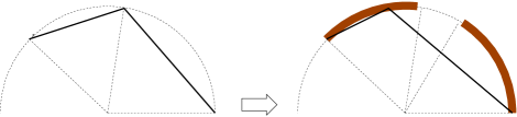
Figure 5: The RG flow $\Scr{B}_{L_{1}}\oplus\Scr{B}_{L_{2}}\rightarrow\Scr{B}_{{L_{1}+L_{2}\over 2}+j+1}\oplus\Scr{B}_{{L_{1}+L_{2}\over 2}-j-1}$ generated by the operator corresponding to $|j\rangle_{L_{1}L_{2}}^{f}$ or $|j\rangle_{L_{2}L_{1}}^{f}$. The mid-point after the flow can only be in the shaded regions. The two components correspond to whether the flow is generated by $|j\rangle_{L_{1}L_{2}}^{f}$ or $|j\rangle_{L_{2}L_{1}}^{f}$. It is evident that the sum of lengths decreases under the flow.

Finally, we would like to comment on operators in the $\Scr{B}_{L_{i}}$-$\Scr{B}_{L_{i}}$ sectors. As we have seen, there are indeed fermionic chiral primary operators that may correspond to relevant deformations. However, one cannot find a deformation that obeys the supersymmetry condition $f(x)g(x)=-iW$ and $g(x)f(x)=-iW$. Thus, it seems that these operators cannot induce a finite supersymmetric deformation of the system. This guarantees the conservation of the torsion D-brane charge $\Lambda_{B}\cong{\mathbb{Z}}_{k+2}$ we have claimed.

5 B-Branes in LG Orbifold $W=X^{k+2}/{\mathbb{Z}}_{k+2}$

In this section, we study the charges and the boundary RG flows for B-branes in the LG orbifold of $W=X^{k+2}$ with respect to the group ${\mathbb{Z}}_{k+2}$ generated by $\gamma:X\rightarrow\omega X$. This is mirror to A-branes in the LG model without orbifold which are studied in [18]. We first describe that known cases and then see how the result is reproduced and extended using B-branes of the orbifold.

5.1 Mirror picture: A-branes in $W=\widetilde{X}^{k+2}$

We recall that we have an A-brane $\Scr{A}_{L,M}$ in the LG model $W=\widetilde{X}^{k+2}$ for each $(L,M)$ with $L+M=1$ is even. It is the wedge coming from $\arg(\widetilde{x})=\pi{M-L-1\over k+2}$ and going to $\arg(\widetilde{x})=\pi{M+L+1\over k+2}$ (see Figure 2). The Witten index of the open string stretched between two of such branes is

$$I(\Scr{A}_{1},\Scr{A}_{2})=\#(\Scr{A}_{1}^{-}\cap\Scr{A}_{2}^{+})$$ (5.1)

where $\Scr{A}^{\pm}$ is the rotation of $\Scr{A}$ by a small positive/negative angle (see [23]). The space of supersymmetric ground states of the string is

$${\mathcal{H}}^{b}_{\rm SUSY}\oplus{\mathcal{H}}^{f}_{\rm SUSY}=\left\{\begin{array}[]{ll}{\mathbb{C}}\oplus 0&{\rm if}\,\,I=1\\ 0\oplus{\mathbb{C}}&{\rm if}\,\,I=-1\\ 0\oplus 0&{\rm if}\,\,I=0.\end{array}\right.$$ (5.2)

If $L_{1}\geq L_{2}$, $k\geq L_{1}+L_{2}$, the index is given by

$$I(\Scr{A}_{L_{1},M_{1}},\Scr{A}_{L_{2},M_{2}})=\left\{\begin{array}[]{ll}\,\,1&{\rm if}\,\,\,{M_{2}-L_{2}-1\over 2}+1\leq{M_{1}+L_{1}+1\over 2}\leq{M_{2}+L_{2}+1\over 2}\\[5.69046pt] \,-1&{\rm if}\,\,\,{M_{2}-L_{2}-1\over 2}+1\leq{M_{1}-L_{1}-1\over 2}\leq{M_{2}+L_{2}+1\over 2}\\[5.69046pt] \,\,0&\mbox{otherwise}.\end{array}\right.$$ (5.3)

The charge lattice of the A-branes is $H_{1}({\mathbb{C}},B^{+})$ where $B^{+}$ is the region in which ${\rm Im}(W)$ is large positive. It is

$$\Lambda_{A}\cong{\mathbb{Z}}^{k+1}$$ (5.4)

generated by $[\Scr{A}^{+}_{0,M}]$ $M=0,2,...,2(k+1)$ which obey the linear relation

$$[\Scr{A}^{+}_{0,0}]+[\Scr{A}^{+}_{0,2}]+\cdots+[\Scr{A}^{+}_{0,2k+2}]=0\qquad{\rm in}\,\,\,H_{1}({\mathbb{C}},B^{+}).$$

Figure 6 describes this relation in the example of $k=6$.

Figure 6: The branes $\Scr{A}_{0,M}$, $M=0,2,...,2(k+1)$ (for the case $k=6$). The shaded regions are $B^{+}$. With a small positive rotation, each represent a class $[\Scr{A}_{0,M}^{+}]\in H_{1}({\mathbb{C}},B^{+})$. The sum annihilates in $H_{1}({\mathbb{C}},B^{+})$ because of the cancellation of the out-going ray of one brane and the in-coming ray of the next brane.

5.1.1 RG-flow as brane recombination

Let us study the supersymmetric boundary RG flows. We first consider a single brane $\Scr{A}_{L,M}$. This represents a non-trivial charge $[\Scr{A}_{L,M}^{+}]\in H_{1}({\mathbb{C}},B^{+})$ and must be stable. Indeed, since $I(\Scr{A}_{L,M},\Scr{A}_{L,M})=1$, there is only one supersymmetric ground state and it is bosonic. Therefore there is no fermionic chiral primary field and hence no supersymmetric deformation operator. We next consider the sum of two branes $\Scr{A}_{L_{1},M_{1}}\oplus\Scr{A}_{L_{2},M_{2}}$. Whether there is another brane configuration to which it can decay depends on the intersection numbers of the two branes. There are four cases to consider.

(i) No intersection
If the two do not intersect, there is no supersymmetric ground state, and hence no supersymmetric deformation of the brane configuration, both in the 1-2 and 2-1 string sectors. Since there is neither in the 1-1 and 2-2 sectors (as we have seen for the single brane case), there is no supersymmetric deformation of the brane. Thus the brane is stable.

(ii) “Transverse” intersection
This is the case where the two intersects transversely as in Figure 7(Left).

Figure 7: Two branes intersecting “transversely” (Left). It is expected to recombine to two other branes without intersection (Right).

In this case, one of the intersection numbers is $+1$ and other is $-1$. In the Figure it is $I(1,2)=1$ and $I(2,1)=-1$. In this case, there is one fermionic supersymmetric ground state in the 2-1 string sector. Depending on the dimension of the corresponding deformation operator, the brane can decay into another brane configuration. The wedge-picture suggests that the brane recombination occurs, and it ends up with a configuration of two other branes. The end point is as in Figure (Right) which is the sum $\Scr{A}_{L_{1}^{\prime},M_{1}^{\prime}}\oplus\Scr{A}_{L_{2}^{\prime},M_{2}^{\prime}}$, where $L_{1}^{\prime}={L_{1}+L_{2}-M_{1}+M_{2}\over 2},M_{1}^{\prime}={-L_{1}+L_{2}+M_{1}+M_{2}\over 2},$ $L_{2}^{\prime}={L_{1}+L_{2}+M_{1}-M_{2}\over 2},M_{2}^{\prime}={L_{1}-L_{2}+M_{1}+M_{2}\over 2}$.

(iii) “Non-transverse” intersection, $-1$
If the incoming ray of one wedge is the same as the out-going ray of the other, one of the intersections is $0$ but the other is $\pm 1$ depending on the orientations of the two branes. Here we consider the $-1$ case, as in Figure 8(Left) where $I(1,2)=0$ and $I(2,1)=-1$.

Figure 8: Two branes intersecting “non-transversely” (Left). They are expected to combine into one brane (Right) by canceling the parallel rays of opposite orientation.

In this case, there is one fermionic supersymmetric ground state from the 2-1 string sector. If the dimension of the corresponding deformation operator is less than 1, it can decay to a new brane configuration. The wedge-picture suggests it is the brane obtained by deleting the overlapping and oppositely oriented rays of the two branes. For the case as in Figure where $\pi{M_{1}+L_{1}+1\over k+2}=\pi{M_{2}-L_{2}-1\over k+2}$ (mod $2\pi$) and $L_{1}+L_{2}\leq k$, it is $\Scr{A}_{L,M}$ with $L=L_{1}+L_{2}+1$ and $M={-L_{1}+L_{2}+M_{1}+M_{2}\over 2}$.

(iv) “Non-transverse” intersection, $+1$
Next, we consider the $+1$ case, as in Figure 9 where $I(1,2)=0$ and $I(2,1)=1$, which is obtained by flipping the orientation of one of the two branes.

Figure 9: Two branes intersecting “non-transversely”. They cannot combine into one brane because the orientation of the parallel rays are the same.

In this case, there is one bosonic ground state but no fermionic ground state. Thus, there is no supersymmetric deformation and the brane is stable.

5.2 B-branes in the orbifold

We now describe the same system in the mirror LG orbifold.

Let us denote by $\Scr{B}_{L,M}$ the B-brane in the orbifold obtained from the B-brane $(\Scr{B}_{L},\rho_{M})$ of the original model where $\rho_{M}$ is the Chan-Paton representation of the orbifold group ${\mathbb{Z}}_{k+2}$ given by (3.12),

$$\gamma:|0\rangle_{L}\mapsto\omega^{-{M+L+1\over 2}}|0\rangle_{L},\quad\overline{\eta}|0\rangle_{L}\mapsto\omega^{-{M-L-1\over 2}}\overline{\eta}|0\rangle_{L}.$$

Note that the “brane configuration” $({\mathbb{C}}\overline{\eta}|0\rangle_{L}\mathop{\rightleftharpoons}^{\!\!\!\!\!\!f}_{\!\!\!\!\!\!g}{\mathbb{C}}|0\rangle_{L})$ is invariant under the orbifold group

$$f(x)=x^{L+1}\rightarrow\omega^{-{M+L+1\over 2}}f(\omega x)\omega{M-L-1\over 2}=f(x),$$

$$g(x)=x^{k+1-L}\rightarrow\omega^{-{M-L-1\over 2}}g(\omega x)\omega^{M+L+1\over 2}=g(x).$$

5.2.1 Open string ground states

Let us first analyze the supersymmetric ground states of the open string stretched between two such branes, $\Scr{B}_{L_{1},M_{2}}$ and $\Scr{B}_{L_{2},M_{2}}$. First thing to note is that the ${\mathbb{Z}}_{k+2}$-equivariant $\overline{Q}$-cohomology is the same as the ${\mathbb{Z}}_{k+2}$-invariant states of the ordinary $\overline{Q}$-cohomology. Let us explain this. Let $(C,Q)$ be a complex and let $\Gamma$ be a symmetry group. Namely $\Gamma$ acts on $C$ and each $\gamma\in\Gamma$ preserves the degree and commutes with $Q$. Then, the $\Gamma$-invariant elements of $C$ form a complex $C^{\Gamma}$. We assume $\Gamma$ is a compact group. Then we have a

Theorem. $\Gamma$-invariant part of the cohomology group is the same as the cohomology of $\Gamma$-invariant part of the complex

$$H(C,Q)^{\Gamma}=H(C^{\Gamma},Q).$$ (5.5)

Proof: The proof assumes that $\Gamma$ is finite but it is clear this applies also to a group with an invariant measure with volume 1. We have a map

$$Z^{\Gamma}\longrightarrow(Z/QC)^{\Gamma}.$$ (5.6)

We want to show (i) it is surjective, and (ii) the Kernel is $Q(C^{\Gamma})$. To show (i) let $f\in C$ represent a $\Gamma$-invariant cohomology class. Namely, $Qf=0$ and, for any $\gamma\in\Gamma$, $\gamma f=f+Qf^{\prime}_{\gamma}$ for some $f^{\prime}_{\gamma}\in C$. Then,

$$f_{1}:={1\over|\Gamma|}\sum_{\gamma\in\Gamma}\gamma f=f+Qf^{\prime}$$

for some $f^{\prime}\in C$. Namely, $f\equiv f_{1}\in Z^{\Gamma}$. This shows (i). To show (ii), let $f\in Z^{\Gamma}$ be mapped to $0$ by (5.6). Namely, $\gamma f=f(\forall\gamma\in\Gamma)$, $Qf=0$, and $f=Qf^{\prime}$ for some $f^{\prime}\in C$. Then,

$$f={1\over|\Gamma|}\sum_{\gamma\in\Gamma}\gamma f={1\over|\Gamma|}\sum_{\gamma\in\Gamma}\gamma Qf^{\prime}=Q\left({1\over|\Gamma|}\sum_{\gamma\in\Gamma}\gamma f^{\prime}\right).$$

This means $f\in Q(C^{\Gamma})$. Thus (ii) is shown. End.

The orbifold group action on the supersymmetric ground states of the original theory have been found in (3.13). There is at most one invariant state. It is $|j_{*}\rangle_{L_{1}L_{2}}^{b}$ or $|j_{*}^{\prime}\rangle_{L_{1}L_{2}}^{f}$ if $j_{*}$ or $j_{*}^{\prime}$ defined by

$$j_{*}\equiv{M_{2}-M_{1}\over 2},\qquad j_{*}^{\prime}\equiv{M_{1}-M_{2}\over 2}-1\qquad\mbox{mod $(k+2)$},$$

is in the range (3.10), and there is none if both of them are outside that range. Thus, we find

$${\mathcal{H}}^{b}_{\rm SUSY}\oplus{\mathcal{H}}^{f}_{\rm SUSY}=\left\{\begin{array}[]{ll}{\mathbb{C}}\oplus 0&{\rm if}\,\,{|L_{1}-L_{2}|\over 2}\leq\Bigl{[}{M_{2}-M_{1}\over 2}\Bigr{]}_{k+2}\leq\min\Bigl{\{}{L_{1}+L_{2}\over 2},k-{L_{1}+L_{2}\over 2}\Bigr{\}}\\[5.69046pt] 0\oplus{\mathbb{C}}&{\rm if}\,\,{|L_{1}-L_{2}|\over 2}\leq\Bigl{[}{M_{1}-M_{2}\over 2}-1\Bigr{]}_{k+2}\leq\min\Bigl{\{}{L_{1}+L_{2}\over 2},k-{L_{1}+L_{2}\over 2}\Bigr{\}}\\[5.69046pt] 0\oplus 0&\mbox{otherwise},\end{array}\right.$$ (5.7)

where $[c]_{k+2}$ is the lowest non-negative number in $c+(k+2){\mathbb{Z}}$. This agrees with the ground state spectrum for the pair $\Scr{A}_{L_{1},M_{1}}$-$\Scr{A}_{L_{2},M_{2}}$. For example, compare with (5.3) for the case $L_{1}\geq L_{2}$ and $k\geq L_{1}+L_{2}$. Thus we find the following identification

$$\Scr{A}_{L,M}=\Scr{B}_{L,M}.$$ (5.8)

What we learn from this is the dimension of the operator $\Scr{O}$ for the supersymmetric deformations. The identification given in Section 3 of the R-charge of the ground states and corresponding operators goes through without modification also in the orbifold theory. In particular, the dimension of the operator that corresponds to the fermionic supersymmetric ground state (present in the middle case of (5.7)) is

$$\Delta={k+1-j_{*}^{\prime}\over k+2}\equiv 1-{M_{1}-M_{2}\over 2(k+2)}\,\,\,\mbox{mod $(k+2)$}.$$ (5.9)

It is indeed a relevant operator, $\Delta<1$.

5.2.2 RG flows

Let us consider the sum of two branes $\Scr{B}_{L_{1},M_{1}}\oplus\Scr{B}_{L_{2},M_{2}}$. The Chan-Paton factor is given by ${\mathbb{C}}^{2}_{+}\oplus{\mathbb{C}}^{2}_{-}$ where ${\mathbb{C}}^{2}_{+}$ is spanned by $\{|0\rangle_{L_{1}},|0\rangle_{L_{2}}\}$ and ${\mathbb{C}}^{2}_{-}$ is spanned by $\{\overline{\eta}_{1}||0\rangle_{L_{1}},\overline{\eta}_{2}|0\rangle_{L_{2}}\}$ on which the orbifold group acts as

$$\gamma_{+}=\left(\begin{array}[]{cc}\omega^{-{M_{1}+L_{1}+1\over 2}}&0\\ 0&\omega^{-{M_{2}+L_{2}+1\over 2}}\end{array}\right),\quad\gamma_{-}=\left(\begin{array}[]{cc}\omega^{-{M_{1}-L_{1}-1\over 2}}&0\\ 0&\omega^{-{M_{2}-L_{2}-1\over 2}}\end{array}\right),$$

respectively. The maps $f:{\mathbb{C}}^{2}_{-}\rightarrow{\mathbb{C}}^{2}_{+}$ and $g:{\mathbb{C}}^{2}_{+}\rightarrow{\mathbb{C}}^{2}_{-}$ are represented by the matrices

$$f(x)=\left(\begin{array}[]{cc}x^{L_{1}+1}&0\\ 0&x^{L_{2}+1}\end{array}\right),\quad g(x)=\left(\begin{array}[]{cc}x^{k+1-L_{1}}&0\\ 0&x^{k+1-L_{2}}\end{array}\right),$$

which are indeed invariant under the orbifold group action, $f(x)\rightarrow\gamma_{+}f(\omega x)\gamma_{-}^{-1}$, $g(x)\rightarrow\gamma_{-}g(\omega x)\gamma_{+}^{-1}$. We would like to identify the supersymmetric deformation given by the relevant operator corresponding to $|j_{*}^{\prime}\rangle_{L_{1}L_{2}}^{f}$ when it is present. Let us try the family of configurations given by (4.56) and (4.64):

$$f_{t}(x) = \left(\begin{array}[]{cc}x^{L_{1}+1}\cos t&x^{L_{2}+1-a}\sin t\\ -x^{L_{1}+1+a}\sin t&x^{L_{2}+1}\cos t\end{array}\right),$$ (5.12)

$$g_{t}(x) = \left(\begin{array}[]{cc}x^{k+1-L_{1}}\cos t&-x^{k+1-L_{1}-a}\sin t\\ x^{k+1-L_{2}+a}\sin t&x^{k+1-L_{2}}\cos t\end{array}\right)$$ (5.15)

where $a$ is an integer such that

$${\rm max}\{-L_{1}-1,\,L_{2}-k-1\}\leq a\leq{\rm min}\{L_{2}+1,\,k+1-L_{1}\}.$$ (5.16)

In the present case, we need to make sure that the deformation is invariant under the orbifold group ${\mathbb{Z}}_{k+2}$ which acts as $f_{t}(x)\rightarrow\gamma_{+}f_{t}(\omega x)\gamma_{-}^{-1}$, $g_{t}(x)\rightarrow\gamma_{-}g_{t}(\omega x)\gamma_{+}^{-1}$. This requires the condition

$$\omega^{a}=\omega^{M_{2}+L_{2}-M_{1}-L_{1}\over 2}.$$ (5.17)

If $j_{*}^{\prime}$ is in the allowed range (3.10), one can solve (5.17) for $a$ within (5.16). Then it is clear that $f_{\varepsilon}(x),g_{\varepsilon}(x)$ can be regarded as the perturbation by the operator corresponding to the state $|j_{*}^{\prime}\rangle_{L_{1}L_{2}}$ (cf. Section 4.3). The perturbed theory flows in the IR limit to the configuration with $t={\pi\over 2}$. After the basis change of ${\mathbb{C}}^{2}_{+}$ by $R_{\pi\over 2}={0\,-1\choose\!1\,\,\,\,0}$, it is given by

$$f^{\prime}(x)=\left(\begin{array}[]{cc}x^{L_{1}+a+1}&0\\ 0&x^{L_{2}-a+1}\end{array}\right),\quad g^{\prime}(x)=\left(\begin{array}[]{cc}x^{k-L_{1}-a+1}&0\\ 0&x^{k-L_{2}+a+1}\end{array}\right)$$ (5.22)

$$\gamma_{+}^{\prime}=\left(\begin{array}[]{cc}\omega^{-{M_{2}+L_{2}+1\over 2}}&0\\ 0&\omega^{-{M_{1}+L_{1}+1\over 2}}\end{array}\right),\quad\gamma_{-}^{\prime}=\gamma_{-}.$$ (5.25)

This is the configuration for $\Scr{B}_{L_{1}^{\prime},M_{1}^{\prime}}\oplus\Scr{B}_{L_{2}^{\prime},M_{2}^{\prime}}$ where

$$L_{1}^{\prime}=L_{1}+a\equiv\mbox{${L_{1}+L_{2}-M_{1}+M_{2}\over 2}$ (mod $k+2$)},\quad M_{1}^{\prime}=\mbox{${-L_{1}+L_{2}+M_{1}+M_{2}\over 2}$},$$ (5.26)

$$L_{2}^{\prime}=L_{2}-a\equiv\mbox{${L_{1}+L_{2}+M_{1}-M_{2}\over 2}$ (mod $k+2$)},\quad M_{2}^{\prime}=\mbox{${L_{1}-L_{2}+M_{1}+M_{2}\over 2}$}.$$ (5.27)

Thus, we found that the deformation by the operator corresponding to $|j_{*}^{\prime}\rangle_{L_{1}L_{2}}^{f}$ generates the RG flow

$$\Scr{B}_{L_{1},M_{1}}\oplus\Scr{B}_{L_{2},M_{2}}\,\longrightarrow\,\Scr{B}_{L_{1}^{\prime},M_{1}^{\prime}}\oplus\Scr{B}_{L_{2}^{\prime},M_{2}^{\prime}}$$ (5.28)

where the two sets of labels are related by (5.26) and (5.27). The decrease of the boundary entropy can be shown in the same way as in Section 4.3. This process is the mirror of the brane-recombination of the A-branes as described in Case (ii) of Section 5.1.1, see Figure 7. This is enough to see that the brane charge is generated by $\Scr{B}_{0,M}$ with $M=0,2,...,2(k+1)$ which are related by

$$[\Scr{B}_{0,0}]+[\Scr{B}_{0,2}]+\cdots+[\Scr{B}_{0,2k+2}]=0.$$

The mirror of Case (iii) where two branes $\Scr{A}_{L_{1},M_{1}}\oplus\Scr{A}_{L_{2},M_{2}}$ combine into one $\Scr{A}_{L,M}$ is described by the flow with $a=L_{2}+1$. The ${\mathbb{Z}}_{k+2}$-invariance condition (5.17) in this case is nothing but $\pi{M_{1}+L_{1}+1\over k+2}\equiv\pi{M_{2}-L_{2}-1\over k+2}$ (mod $2\pi$), which is the condition that the out-going ray of $\Scr{A}_{L_{1},M_{1}}$ agrees with the in-coming ray of $\Scr{A}_{L_{2},M_{2}}$.

References

• [1]
• [2] A. B. Zamolodchikov and V. A. Fateev, “Disorder fields in two-dimensional conformal quantum field theory and N=2 extended supersymmetry”, Sov. Phys. JETP 63 (1986) 913 [Zh. Eksp. Teor. Fiz.  90 (1986) 1553].
• [3] Z. Qiu, “Nonlocal current algebra and N=2 superconformal field theory in two-dimensions”, Phys. Lett. B 188 (1987) 207.
• [4] M. Ademollo et al., “Supersymmetric strings and color confinement”, Phys. Lett. B 62 (1976) 105; “Dual string with U(1) color symmetry”, Nucl. Phys. B 111 (1976) 77.
• [5] F. Ravanini and S. K. Yang, “Modular invariance in N=2 superconformal field theories”, Phys. Lett. B 195 (1987) 202.
• [6] Z. Qiu, “Modular invariant partition functions for N=2 superconformal field theories”, Phys. Lett. B 198 (1987) 497.
• [7] E. J. Martinec, “Algebraic Geometry And Effective Lagrangians,” Phys. Lett. B 217 (1989) 431; “Criticality, Catastrophes And Compactifications,” In Brink, L. (ed.) et al.: Physics and mathematics of strings, V.G. Knizhnik memorial vol. 389-433.
• [8] C. Vafa and N. P. Warner, “Catastrophes And The Classification Of Conformal Theories,” Phys. Lett. B 218 (1989) 51.
• [9] E. Witten, “On the Landau-Ginzburg description of N=2 minimal models,” Int. J. Mod. Phys. A 9 (1994) 4783 [hep-th/9304026].
• [10] J. A. Harvey, D. Kutasov and E. J. Martinec, “On the relevance of tachyons,” hep-th/0003101.
• [11] A. Sen, “Non-BPS states and branes in string theory,” hep-th/9904207.
• [12] A. Sen and B. Zwiebach, “Tachyon condensation in string field theory,” JHEP 0003 (2000) 002 [hep-th/9912249].
• [13] A. A. Gerasimov and S. L. Shatashvili, “On exact tachyon potential in open string field theory,” JHEP 0010 (2000) 034 [hep-th/0009103]; D. Kutasov, M. Marino and G. W. Moore, “Some exact results on tachyon condensation in string field theory,” JHEP 0010 (2000) 045 [hep-th/0009148].
• [14] E. Witten, “D-branes and K-theory,” JHEP 9812 (1998) 019 [hep-th/9810188].
• [15] M. R. Douglas, “D-branes, categories and N = 1 supersymmetry,” J. Math. Phys.  42 (2001) 2818 [hep-th/0011017].
• [16] J. McGreevy and H. Verlinde, “Strings from tachyons: The c = 1 matrix reloaded,” JHEP 0312 (2003) 054 [hep-th/0304224]; I. R. Klebanov, J. Maldacena and N. Seiberg, “D-brane decay in two-dimensional string theory,” JHEP 0307 (2003) 045 [hep-th/0305159].
• [17] A. Sen, “Rolling tachyon,” JHEP 0204 (2002) 048 [hep-th/0203211]; M. Gutperle and A. Strominger, “Spacelike branes,” JHEP 0204 (2002) 018 [hep-th/0202210]; N. Lambert, H. Liu and J. Maldacena, “Closed strings from decaying D-branes,” hep-th/0303139.
• [18] K. Hori, A. Iqbal and C. Vafa, “D-branes and mirror symmetry,” hep-th/0005247.
• [19] J. M. Maldacena, G. W. Moore and N. Seiberg, “Geometrical interpretation of D-branes in gauged WZW models,” JHEP 0107 (2001) 046 [hep-th/0105038].
• [20] K. D. Kennaway, “A geometrical construction of Recknagel-Schomerus boundary states in linear sigma models,” Nucl. Phys. B 647 (2002) 471 [hep-th/0203266].
• [21] S. Fredenhagen and V. Schomerus, “D-branes in coset models,” JHEP 0202 (2002) 005 [hep-th/0111189]; “On boundary RG-flows in coset conformal field theories,” Phys. Rev. D 67 (2003) 085001 [hep-th/0205011]; S. Fredenhagen, “Organizing boundary RG flows,” Nucl. Phys. B 660 (2003) 436 [hep-th/0301229].
• [22] K. Hori, “Linear models of supersymmetric D-branes,” hep-th/0012179.
• [23] K. Hori, S. Katz, A. Klemm, R. Pandharipande, R. Thomas, C. Vafa, R. Vakil and E. Zaslow, Mirror Symmetry, (AMS-CMI, 2003).
• [24] K. Hori, “Mirror symmetry and quantum geometry,” hep-th/0207068.
• [25] A. Kapustin and Y. Li, “D-branes in Landau-Ginzburg models and algebraic geometry,” JHEP 0312 (2003) 005 [hep-th/0210296]; “Topological correlators in Landau-Ginzburg models with boundaries,” hep-th/0305136; “D-branes in topological minimal models: The Landau-Ginzburg approach,” hep-th/ 0306001.
• [26] D. Orlov, “Triangulated categories of singularities and D-branes in Landau-Ginzburg models,” math.ag/0302304.
• [27] I. Brunner, M. Herbst, W. Lerche and B. Scheuner, “Landau-Ginzburg realization of open string TFT,” hep-th/0305133.
• [28] C. I. Lazaroiu, “On the boundary coupling of topological Landau-Ginzburg models,” hep-th/0312286.
• [29] M. F. Atiyah, K-theory Benjamin, New York, 1967.
• [30] A. Cappelli, G. D’Appollonio and M. Zabzine, “Landau-Ginzburg description of boundary critical phenomena in two dimensions,” hep-th/0312296.
• [31] S. A. Ashok, E. Dell’Aquila and D. E. Diaconescu, “Fractional Branes in Landau-Ginzburg Orbifolds,” hep-th/0401135.
• [32] H. Ooguri, Y. Oz and Z. Yin, “D-branes on Calabi-Yau spaces and their mirrors,” Nucl. Phys. B 477 (1996) 407 [hep-th/9606112].
• [33] S. Govindarajan, T. Jayaraman and T. Sarkar, “Worldsheet approaches to D-branes on supersymmetric cycles,” Nucl. Phys. B 580 (2000) 519 [hep-th/9907131].
• [34] N. P. Warner, “Supersymmetry in boundary integrable models,” Nucl. Phys. B 450 (1995) 663 [hep-th/9506064].
• [35] S. Hellerman, S. Kachru, A. E. Lawrence and J. McGreevy, “Linear sigma models for open strings,” JHEP 0207 (2002) 002 [hep-th/0109069].
• [36] T. Takayanagi, S. Terashima and T. Uesugi, “Brane-antibrane action from boundary string field theory,” JHEP 0103 (2001) 019 [hep-th/0012210].
• [37] P. Kraus and F. Larsen, “Boundary string field theory of the DD-bar system,” Phys. Rev. D 63 (2001) 106004 [hep-th/0012198].
• [38] K. Hori and C. Vafa, “Mirror Symmetry,” hep-th/0002222.
• [39] C.-H. Cho and Y.-G. Oh, “Floer cohomology and disc instantons of Lagrangian torus fibers in Fano toric manifolds,” math.SG/0308225.
• [40] C.-H. Cho, “Holomorphic disc, spin structures and Floer cohomology of the Clifford torus,” math.SG/0308224.
• [41] W. Lerche, C. Vafa and N. P. Warner, “Chiral Rings In N=2 Superconformal Theories,” Nucl. Phys. B 324 (1989) 427.
• [42] I. Brunner and K. Hori, “Orientifolds and mirror symmetry,” hep-th/0303135.
• [43] J. L. Cardy, “Boundary Conditions, Fusion Rules And The Verlinde Formula,” Nucl. Phys. B 324 (1989) 581.
• [44] I. Affleck and A. W. W. Ludwig, “Universal Noninteger ’Ground State Degeneracy’ In Critical Quantum Systems,” Phys. Rev. Lett.  67 (1991) 161.
• [45] I. Brunner, K. Hori, K. Hosomichi and J. Walcher, “Orientifolds of Gepner Models”, hep-th/0401137.
• [46] C. Vafa, “String Vacua And Orbifoldized L-G Models,” Mod. Phys. Lett. A 4 (1989) 1169.
• [47] A. Sen, “Tachyon condensation on the brane antibrane system,” JHEP 9808 (1998) 012 [hep-th/9805170].
• [48] C. G. Callan, I. R. Klebanov, A. W. W. Ludwig and J. M. Maldacena, “Exact solution of a boundary conformal field theory,” Nucl. Phys. B 422 (1994) 417 [hep-th/9402113].
• [49] J. Polchinski and L. Thorlacius, “Free Fermion Representation Of A Boundary Conformal Field Theory,” Phys. Rev. D 50 (1994) 622 [hep-th/9404008].
• [50] P. Fendley, H. Saleur and N. P. Warner, “Exact solution of a massless scalar field with a relevant boundary interaction,” Nucl. Phys. B 430 (1994) 577 [hep-th/9406125].
• [51] I. Affleck and A. W. W. Ludwig, “Exact conformal-field-theory results on the multichannel Kondo effect: Single-fermion Green’s function, self-energy, and resisitivity,” Phys. Rev. B 48 (1993) 7297.
• [52] D. Kutasov, “New results on the ’a-theorem’ in four dimensional supersymmetric field theory,” hep-th/0312098.