hep-th/0401137 CERN-PH-TH/2004-006 KCL-MTH-04-01 NSF-KITP-04-01

Orientifolds of Gepner Models
Ilka Brunner^∗, Kentaro Hori^†, Kazuo Hosomichi^† and Johannes Walcher^‡

^∗CERN Theory Division, Geneva, Switzerland
and
King’s College, London, United Kingdom
^†University of Toronto, Toronto, Ontario, Canada
^‡Kavli Institute for Theoretical Physics, University of California, Santa Barbara, USA

We systematically construct and study Type II Orientifolds based on Gepner models which have ${\mathcal{N}}=1$ supersymmetry in $3+1$ dimensions. We classify the parity symmetries and construct the crosscap states. We write down the conditions that a configuration of rational branes must satisfy for consistency (tadpole cancellation and rank constraints) and spacetime supersymmetry. For certain cases, including Type IIB orientifolds of the quintic and a two parameter model, one can find all solutions in this class. Depending on the parity, the number of vacua can be large, of the order of $10^{10}-10^{13}$. For other models, it is hard to find all solutions but special solutions can be found — some of them are chiral. We also make comparison with the large volume regime and obtain a perfect match. Through this study, we find a number of new features of Type II orientifolds, including the structure of moduli space and the change in the type of O-planes under navigation through non-geometric phases.

1 Introduction

String vacua with $\mathcal{N}=1$ supersymmetry in $3+1$ spacetime dimensions have been re-attracting a lot of attention in recent years. One of the reasons is of course that despite a lot of efforts spent on the heterotic string, actual connections with real world particle physics have proven difficult to make, and that new avenues have opened up with our growing mastery of strings, branes, and M-theory. But we may also wish to turn this quest around and ask for general lessons from exploring the duality web with four supercharges, which on general grounds is expected to be quite complex. Whether or not one will be able to make contact with phenomenology, or extrapolate to a situation with broken supersymmetry, it is natural to expect that something interesting will be learned.

Type II orientifolds with branes and fluxes are an important class of models. By a chain of duality, they can be related to many other classes of models, including the heterotic string on Calabi-Yau 3-folds and M-theory on $G_{2}$-holonomy manifolds, and therefore may possibly provide a unifying scheme for $4d$ ${\mathcal{N}}=1$ compactifications [2]. They provide natural set-ups for the braneworld scenario. It should also be noted that the recent progress in moduli stabilization is done in this framework [3, 4]. However, most of the study in the past is done using supergravity, or only toroidal orientifolds are given serious accounts. This is definitely not a satisfactory state of affairs, because the large volume or flat backgrounds are a tiny part of the whole variety of possible theories. What we need is a handle on the regime where supergravity is not accessible.

In this paper, we study the other extreme regime where the internal space is very small but nevertheless the worldsheet is extremely powerful. Namely, we construct and study Type II orientifolds based on Gepner models [5]. We will also try to see how such theories are connected to the large volume regimes.

To avoid confusion, we emphasize that what we do here is within the framework of the perturbative NSR formalism. We are obviously not able to include (RR) fluxes, and we are not going to discuss the stringy quantum corrections at this stage, except in the discussion of the anomaly cancellation mechanism and Fayet-Iliopoulos terms. In particular, the moduli including the dilaton remain unfixed. However, we want to regard our work as a useful starting point for an explicit study of such models. For instance, our models will have non-abelian gauge groups living on various RR tadpole canceling branes, and our results may be useful also for the final step in the moduli stabilization [4].

In fact, the roads have been partially paved for us. Recently, a great deal of results on D-branes in Type II string compactifications were obtained. They include application of Cardy’s RCFT techniques [7] and also the study of how they continue in the moduli space to the large volume [8]. There is also an orientifold version of Cardy, initiated by Pradisi-Sagnotti-Stanev [9] and further developed by many people [10, 11, 12, 13, 15]. Some of the preliminary results have been obtained in [16, 17] and more recently in [18, 19, 20]. In particular, we will extensively use the results of [18] on the minimal models and other general properties of orientifolds of $(2,2)$ theories.

Our goal in this paper is threefold. Firstly, we want to adapt and generalize the RCFT methods to the full string theory based on the Gepner models. Secondly, we want to present as unified a view as possible of the various descriptions available for these worldsheets, such as the Landau-Ginzburg and gauged linear sigma model pictures. In particular, we want to generalize the relations between the Gepner point and large volume regimes to the situation involving unoriented strings. Thirdly, we want to give rather detailed lists of explicit models that can be constructed within this framework.

The ripeness of the subject and the richness of the harvest have forced this paper to rather extended length. In order to guide the reader towards the important results, we now give an overview over the organization of the presentation.

According to our global goal, we begin our discussion in section 2 in the context of the gauged linear sigma model (GLSM), which provides the most global picture of Calabi-Yau compactifications on the worldsheet. The discussion in subsection 2.1 is rather standard, and can safely be skipped by experts.

In subsection 2.2, we review the possible orientifold projections, as discussed for example in [18]. As could be expected, parity symmetries of $\mathcal{N}=2$ supersymmetric field theories come in two varieties, called A and B-type respectively. The tadpoles arising from the corresponding O-planes must be canceled by A and B-type D-branes, and the resulting $\mathcal{N}=1$ models can be thought of as Type IIA/IIB orientifolds, respectively. The associated geometries are quite different, but are related to each other by mirror symmetry. Of importance will be the classification of possible dressing of the parity by various (classical and quantum) symmetries of the theory in such a way that the parity is involutive.

In subsection 2.3, we make this discussion concrete in the two examples which will accompany us through the rest of the paper: the quintic hypersurface in ${\mathbb{P}}^{4}$ and the degree $8$ hypersurface in weighted projective space ${\mathbb{P}}^{4}_{1,1,2,2,2}$. As we will see, many interesting features arise in this two parameter model, which admits a much richer set of possible orientifold projections than the quintic. For example, we will see that with the appropriate dressing it is possible to project out the Kähler modulus corresponding to the overall size of the Calabi-Yau, or to select different sections of the moduli space, corresponding to discrete fluxes in the large volume regime.

We have organized the rest of the paper around this division into A and B-type and the illustration in two examples, the quintic and the two parameter model. In section 3, we discuss the construction of crosscap and boundary states in the full worldsheet theory of the Gepner model. Our approach differs slightly from the methods used in the literature [7, 21, 22, 23, 24] in that we use a supersymmetric language throughout. Moreover, our construction of B-type boundary states is new in the sense that it does not use the Greene-Plesser [25] construction of mirror symmetry. This approach also sheds new light on fixed-point resolution or the appearance of so-called short-orbit branes [22, 23, 24, 26].

We are then ready for discussing the consistency conditions that constrain the possible string theory models we can build, A- and B-type in sections 4 and 6, respectively. The discussion includes the computation of O-plane charges, the action of the parities on the D-branes, as well as the structure of Chan-Paton factors. This puts us in a position to solve the consistency conditions explicitly for our two examples. We also discuss the computation of the massless open string spectrum. We conclude each of the sections with lists of solutions to the tadpole cancellation conditions and open string spectra in selected cases.

The possibilities turn out to be extremely numerous and rich. For instance, for B-type models on the quintic, it turns out that there are $31561671503$ different supersymmetric and tadpole canceling configurations of rational branes at the Gepner point, all with the orthogonal gauge groups. The number of vacua is similar in the two parameter model, depending on the parity, with the the additional interesting feature of allowing for configurations with unitary and symplectic gauge groups.

For A-type models, the spectrum is expected to be even richer, although we are not able to solve the tadpole constraints completely in this case. The number of equations and the number of branes are too many for even the computer to find the solutions in a reasonable time. However, special solutions can be found: For any model with odd levels only, we always have a solution consisting of four identical branes — four D6-branes on top of the O6-plane in the large volume limit. For models including even levels, such a solution does not always exist but one can use the recombination of branes in the Landau-Ginzburg model to find special solutions in many cases. Also, the size of the problem is much smaller when we consider “intermediate” models whose orbifold group is not minimal (single cyclic group) nor maximal (the mirror of single-cyclic Gepner model).

Some of the theories we obtain have chiral matter contents. Two out of nine special solutions for the two parameter model (A-type) are chiral. One of them has $U(1)^{8}$ gauge group with chiral quiver matters, and the other is $Sp(1)\times Sp(1)\times U(2)$ theory with matters in $2\times({\bf 2},{\bf 1},{\bf 2})$, $({\bf 1},{\bf 2},\overline{\bf 2})$ and $({\bf 2},{\bf 2},{\bf 1})$. We feel that there are more chiral solutions than these two, but how many and which is not clear at the moment. For Type IIB orientifolds on Gepner models based on a single cyclic group, such as the quintic or the two parameter model, all the solutions are non-chiral. However, some of the randomly chosen solutions of a ${\mathbb{Z}}_{5}$-orbifold of quintic are chiral. Thus, we obtain the first examples of chiral supersymmetric 4d theories out of non-toroidal orientifolds.

Section 5 is an interlude, in which we make remarks on chirality, anomaly cancellation mechanism and Fayet-Iliopoulos terms. The bilinear identity of the Witten index, where the only parity-invariant closed string ground states propagate in the tree channel, plays an essential role in anomaly cancellation. We make explicit the string coupling dependence of the low energy Lagrangian and check that it is consistent with all of the tree level results we obtained.

Finally, in section 7, we compare the results on consistency conditions with the geometrical expectations in the large volume limit, finding complete agreement. We will here make use of the results of [8] and [27] on the connection between geometry and Gepner model boundary states (see also [28, 29, 30, 31]), as well as the results on the structure of the Kähler moduli space of the two parameter model [32] and its real sections discussed in subsection 2.3. We find something interesting through this study: For some Type IIB orientifolds of the two parameter model with two large volume regions (distinguished by the B-field), the type of O-plane changes if one goes from one large volume region to the other, through non-geometric domains of the Kähler moduli space. We consider an example with O5-planes at a genus 9 curve and four rational curves. Here, in one region all O-planes are O5^- (SO-type), whereas in the other region the O-planes at the rational curves become O5⁺ (Sp-type). For Type IIA orientifolds, we find in one example an effective description of closed and open strings that matches the results at the Gepner point as well as large volume. An extensive study needs more technical development such as an A-type analog of [27, 28, 29, 30, 31] (see, however [33]), geometrical study of large volume branes, and methods to compute superpotential in both regimes.

Note: A part of the present work (including Section 3 and a part of Section 4) is presented in a conference in [34]. While the current work was under further progress and was being written, we noticed these papers by Aldazabal et al [35] and by Blumenhagen [36], which have some overlap with our work. However, in these papers, only odd level Gepner models are considered. As we will see, the rich and interesting new physics arises in models including even level minimal models.

2 Calabi-Yau Orientifolds

2.1 Calabi-Yau Sigma Models and Gepner points

Consider a $(2,2)$ supersymmetric gauge theory in $1+1$ dimensions with $U(1)$ gauge group and $r+1$ fields $X_{1},\ldots,X_{r},P$ with tree level superpotential

$$W=P(X_{1}^{k_{1}+2}+\cdots+X_{r}^{k_{r}+2})$$ (2.1)

and twisted superpotential

$$\widetilde{W}=t\Sigma.$$

$\Sigma=\overline{D}_{+}D_{-}V$ is the superfieldstrength and $t=r-i\theta$ is the Fayet-Iliopoulos-Theta parameter. The gauge transformations act on the fields as

$$P\rightarrow\,{\rm e}^{-iH\lambda}P,\quad X_{i}\rightarrow\,{\rm e}^{iw_{i}\lambda}X_{i},$$

where

$$H:={\rm lcm}\{k_{i}+2\},$$

$$w_{i}:={H\over k_{i}+2}.$$

For large values of the FI parameter, the system reduces at low energies to the sigma model on the hypersurface $M=\{X_{1}^{k_{1}+2}+\cdots+X_{r}^{k_{r}+2}=0\}$ in a weighted projective space of dimension $r-1$. This gauge system, introduced in [37], is called the linear sigma model for the manifold $M$. The condition that $M$ is Calabi-Yau is reflected by the vanishing of the sum of charges $-1+\sum_{i=1}^{r}{1\over k_{i}+2}=0$. Namely

$$\sum_{i=1}^{r}{k_{i}\over k_{i}+2}=r-2=\dim M.$$ (2.2)

In this case, the beta function for the FI parameter vanishes and therefore $t$ is a free parameter of the system.

At large negative ${\rm Re}(t)$, the $P$ field has a vacuum expectation value and breaks the $U(1)$ gauge symmetry to the subgroup in which $\,{\rm e}^{iH\lambda}=1$. This unbroken subgroup $\Gamma$ is generated by the one with $\lambda=2\pi/H$ which acts on the fields as

$$\gamma:X_{i}\rightarrow\,{\rm e}^{2\pi i\over k_{i}+2}X_{i},$$ (2.3)

and is a cyclic group of order $H$. The model at $t=-\infty$ is identified as the LG orbifold with superpotential

$$W_{\it G}=X_{1}^{k_{1}+2}+\cdots+X_{r}^{k_{r}+2}$$ (2.4)

divided by the group $\Gamma\cong{\mathbb{Z}}_{H}$ acting on fields as (2.3). The LG model with superpotential $W=X^{k+2}$ flows in the infra-red limit to a $(2,2)$ superconformal field theory with central charge $c={3k\over k+2}$, called the (A-series) level $k$ ${\mathcal{N}}=2$ minimal model, $M_{k}$. The infra-red limit of the above LG orbifold is thus the $\Gamma$-orbifold of the product of the minimal models;

$$\left(\prod_{i=1}^{r}M_{k_{i}}\right)\Biggr{/}\Gamma$$

This is the Gepner model. The generator (2.3) of the orbifold group $\Gamma$ is identified as

$$\gamma=\underbrace{({\it g},\ldots,{\it g})}_{r}$$ (2.5)

in which ${\it g}:=\,{\rm e}^{-2\pi iJ_{0}}(-1)^{\widehat{F}}$ where $J_{0}$ is the $U(1)$ current of the (right-moving) ${\mathcal{N}}=2$ superconformal algebra and $(-1)^{\widehat{F}}$ is $1$ on NSNS sector but $-1$ on RR sector. Note that the RR-ground states of lowest R-charge $q=-{c\over 6}$ survives the orbifold projection, since ${c\over 6}={\dim M\over 2}={r-2\over 2}$ and thus $\gamma=\,{\rm e}^{\pi i(r-2)}(-1)^{r}=1$. This state corresponds to the holomorphic volume form of the Calabi-Yau manifold. We discuss more on the ground states in Section 2.1.1.

Type II string theory on $M\times{\mathbb{R}}^{D}$ is consistent only if $2\dim M+D=10$. If we denote the complex dimension of the transverse space by $d=(D-2)/2$, the criticality condition is

$$r+d=6.$$ (2.6)

In this paper we assume both the Calabi-Yau condition (2.2) and the criticality condition (2.6).

Remarks.
(i) It is possible to have some $k_{i}=0$. The IR limit of $W=X^{2}$ is empty, but can be regarded as the system with a unique (ground) state in each of R/NS-sectors, with zero energy, zero charge. We will regard the $k_{i}=0$ factor as such a quantum field theory. The orbifold group acts on this factor non-trivially: the generator $\gamma$ acts as ${\it g}=\,{\rm e}^{-2\pi iJ_{0}}(-1)^{\widehat{F}}=(-1)^{\widehat{F}}$, namely, as identity on NSNS sector but as $(-1)$ on the RR-sector. Thus, having this factor has a non-trivial effect.
(ii) The behaviour of the system depends very much on whether there is an even $k_{i}$. It is useful to note that when there is at least one even $k_{i}$ there is actually an even number of $i$ with largest factors of $2$ in $k_{i}$, under the Calabi-Yau condition, $\sum_{i=1}^{r}{H\over k_{i}+2}=H$.
(iii) Let us present some examples that satisfy the Calabi-Yau and criticality conditions.
$\bullet$ $(k_{i}+2)=(3,3,3)$; $M=$ an elliptic curve, $D=7+1$.
$\bullet$ $(k_{i}+2)=(4,4,4,4)$; $M=$ a K3 surface. $D=5+1$.
We will mainly consider the case with $r=5$ and $d=1$ since this corresponds to the string compactification to $3+1$ dimensions. The examples of this type are
$\bullet$ $(k_{i}+2)=(5,5,5,5,5)$; $M=$ a quintic hypersurface in ${{\mathbb{C}}{\mathbb{P}}}^{4}$.
$\bullet$ $(k_{i}+2)=(8,8,4,4,4)$.
$\bullet$ $(k_{i}+2)=(8,8,8,8,2)$.
$\bullet$ $(k_{i}+2)=(12,12,6,6,2)$.
The first two will be our basic examples where we examine the general story in detail. A complete list can be found in [38].
(iv) The non-chiral GSO projection of the minimal model $M_{k}$ by $(-1)^{F}=\,{\rm e}^{-\pi i(J_{0}-\widetilde{J}_{0})}$ is the $SU(2)_{k}\times U(1)_{2}$ mod $U(1)$ gauged WZW model, or simply $SU(2)_{k}\times U(1)_{2}/U(1)_{k+2}$ coset model. The latter model has primaries labeled by $(l,m,s)\in{\rm M}_{k}$; namely $l\in P_{k}=\{0,1,...,k\}$, $m\in{\mathbb{Z}}_{2(k+2)}$, $s\in{\mathbb{Z}}_{4}$, with $l+m+s$ even, $(l,m,s)\equiv(k-l,m+k+2,s+2)$. The product theory $M_{k_{1}}\times\cdots\times M_{k_{r}}$ should not be confused with the tensor product of the GSO projected models of $M_{k_{1}},...,M_{k_{r}}$. In the latter the space of states would have mixture of NSNS and RR factors, while in the former NS/R alignment is automatically imposed, as usual in ordinary supersymmetric quantum field theories.
(v) The GSO projected model has global symmetries $g_{n,s}$ corresponding to simple currents $(0,n,s)$ ($n\in{\mathbb{Z}}_{2(k+2)}$, $s\in{\mathbb{Z}}_{4}$, with $n+s$ even) which act on the states in $\Scr{H}_{l^{\prime},m^{\prime},s^{\prime}}\otimes\Scr{H}_{l^{\prime},-m^{\prime},-s^{\prime}}$ as multiplication by a phase $\,{\rm e}^{\pi i\left({nm^{\prime}\over k+2}-{ss^{\prime}\over 2}\right)}$. The symmetry ${\it g}$ above induces one of them, $g_{2,0}$.
(vi) “Gepner Model” usually refers to more general models based on orbifold of the product of minimal models. It doesn’t have to come from linear sigma models of the above types. In Appendix A, we present more general models. In the main text of the paper, we treat only the class of models introduced above (except Sections 3.1 and 3.2 where the discussion is general), in particular the case $D=3+1$ and $r=5$. We relegate the discussion on the most general models to Appendix.

In many cases, $M$ has singularities that are inherited from the orbifold singularities of the ambient space, and their resolution introduces extra Kähler parameters. This is accommodated in the linear sigma model by extending the gauge group and adding charged fields. In general, the gauge group will be $U(1)^{k}=\prod_{a=1}^{k}U(1)_{a}$ gauge theory with matter fields $P,X_{1},\ldots,X_{r+k-1}$ of certain charge $Q_{P}^{a},Q_{1}^{a},\ldots,Q_{r+k-1}^{a}$ and certain (twisted) superpotential. For example, for $(k_{i}+2)=(8,8,4,4,4)$, the full system after the resolution has $U(1)\times U(1)$ gauge group and six matter fields of the following charges [39]:

$$\begin{array}[]{cccccccc}&P&X_{1}&X_{2}&X_{3}&X_{4}&X_{5}&X_{6}\\ U(1)_{1}&-4&0&0&1&1&1&1\\ U(1)_{2}&0&1&1&0&0&0&-2\end{array}$$ (2.7)

The system has superpotential

$$W=P\Bigl{\{}\,X_{6}^{4}(X_{1}^{8}+X_{2}^{8})+X_{3}^{4}+X_{4}^{4}+X_{5}^{4}\,\Bigr{\}},$$

and twisted superpotential

$$\widetilde{W}=t_{1}\Sigma_{1}+t_{2}\Sigma_{2},$$ (2.8)

where the $t_{a}=r_{a}-i\theta_{a}$ and $\Sigma_{a}=\overline{D}_{+}D_{-}V_{a}$ are the FI-Theta parameter and the fieldstrength of the $U(1)_{a}$ gauge group. In the limit $t_{2}\rightarrow-\infty$ with $2t_{1}+t_{2}$ fixed, $X_{6}$ acquires a large absolute value and breaks the gauge group except the one generated by $(2i,i)\in\mathfrak{u}(1)_{1}\oplus\mathfrak{u}(1)_{2}$. We are then left with the original system with one $U(1)$ gauge symmetry whose FI-Theta parameter is $t=2t_{1}+t_{2}$. This corresponds to undoing the resolution.

2.1.1 RR Ground States and Chiral Primaries

Let us present the list of supersymmetric ground states of the system. The level $k$ minimal model has $(k+1)$ supersymmetric ground states $|l\rangle_{{{}_{\rm RR}}}$ ($l=0,1,...,k$) which correspond to $X^{l}$ and have R-charges $q=\widetilde{q}={l+1\over k+2}-{1\over 2}$. Also, on a circle twisted by $\,{\rm e}^{-2\pi i\nu J_{0}}$, there is a unique supersymmetric ground state $|0\rangle_{\nu}$ which has R-charge $q=-\widetilde{q}={l_{\nu}+1\over k+2}-{1\over 2}$ where $l_{\nu}\in\{0,1,...,k\}$ is defined by $l_{\nu}+1\equiv-\nu$ (mod $(k+2)$). The RR ground states of the Gepner model are made of these states. Since the orbifold group is generated by the tensor product of $-\,{\rm e}^{-2\pi iJ_{0}}$ for the $r=5$ factors, the condition is that the sum of R-charges is an odd half-integer, $\sum_{i}q_{i}\in{1\over 2}+{\mathbb{Z}}$. Untwisted sector states are thus the products $\otimes_{i=1}^{5}|l_{i}\rangle_{{{}_{\rm RR}}}$ with the condition $\sum_{i}({l_{i}+1\over k_{i}+2}-{1\over 2})=\sum_{i}{l_{i}\over k_{i}+2}-{3\over 2}\in{1\over 2}+{\mathbb{Z}}$, or

$$\sum_{i=1}^{5}{l_{i}\over k_{i}+2}=0,1,2,3.$$ (2.9)

They correspond to harmonic forms of degree $(3,0)$, $(2,1)$, $(1,2)$ and $(0,3)$ respectively of the relevant Calabi-Yau manifold. There are also RR ground states from the twisted sectors labeled by $\nu=1,2,...,H-1$. The orbifold condition is the same as (2.9) where $l_{i}$ is replaced by $l_{\nu}^{(i)}$ for such $i$ where the twist is non-trivial, $\nu\not\equiv 0$ mod $(k_{i}+2)$. For the $\nu=1$ twist, we find $l_{1}^{(i)}=k_{i}$ for all $i$ and we find a unique ground state with $q=-\widetilde{q}={3\over 2}$. The geometrical counterpart is the $(0,0)$-form. For $\nu=(H-1)$, we also find a unique ground state that corresponds to the $(3,3)$-form. The ground states from the twisted sectors are mostly related to $(p,p)$-forms. However, there can be states corresponding to off-diagonal forms. For example, let us consider the case where $H$ is even and twist by $\nu={H\over 2}$. The twist in the $i$-th factor is non-trivial if and only if $w_{i}={H\over k_{i}+2}$ is odd. For such an $i$, $l_{H\over 2}^{(i)}$ is ${k_{i}\over 2}$ and the ground state is $q_{i}=\widetilde{q}_{i}=0$. For other $i$, the twist is trivial and the ground states are ordinary ones $|l_{i}\rangle_{{{}_{\rm RR}}}$ with R-charges $q_{i}=\widetilde{q}_{i}={l_{i}+1\over k_{i}+2}-{1\over 2}$. They correspond to $(2,1)$ or $(1,2)$ forms. Let us show the number of ground states in two examples.

$(k_{i}+2)=(5,5,5,5,5)$  Untwisted ground states correspond to monomials of $X_{i}$ with degree $0$, $5$, $10$, $15$ (with relations $X_{i}^{4}=0$) and there are $1$, $101$, $101$, $1$ of them. Also there is a unique ground state $\otimes_{i}|0\rangle_{\nu}$ from each of $\nu=1,2,3,4$ twisted sectors. These numbers are organized into the “Hodge diamond”

$$\begin{array}[]{ccccccc}&&&\!\!1\!\!&&&\\[-5.69046pt] &&\!\!0\!\!&&\!\!0\!\!&&\\[-5.69046pt] &\!\!0\!\!&&\!\!1\!\!&&\!\!0\!\!&\\[-5.69046pt] \!\!1\!\!&&\!\!101\!\!&&\!\!101\!\!&&\!\!1\!\!\\[-5.69046pt] &\!\!0\!\!&&\!\!1\!\!&&\!\!0\!\!&\\[-5.69046pt] &&\!\!0\!\!&&\!\!0\!\!&&\\[-5.69046pt] &&&\!\!1\!\!&&&\end{array}$$

$(k_{i}+2)=(8,8,4,4,4)$  $X_{1},X_{2},X_{3},X_{4},X_{5}$ have weights $w_{i}=1,1,2,2,2$. Untwisted ground states correspond to monomials of $X_{i}$ with total weight $0$, $8$, $16$, $24$ (with relations $X_{1}^{7}=X_{2}^{7}=X_{3}^{3}=X_{4}^{3}=X_{5}^{3}=0$). There are $1$, $83$, $83$, $1$ of them. There is a unique ground state $\otimes_{i}|0\rangle_{\nu}$ from each of $\nu=1,2,3,5,6,7$ twisted sectors. They corresponds to diagonal forms. For the $\nu=4$ twisted sector, ground states are

$$\bigotimes_{i=1,2}|0\rangle_{\nu}\otimes\bigotimes_{i=3,4,5}|l_{i}\rangle_{{{}_{\rm RR}}}$$

where $l_{3}+l_{4}+l_{5}=1$ (3 states) or $5$ (3 states). The Hodge diamond is therefore

$$\begin{array}[]{ccccccc}&&&\!\!1\!\!&&&\\[-5.69046pt] &&\!\!0\!\!&&\!\!0\!\!&&\\[-5.69046pt] &\!\!0\!\!&&\!\!2\!\!&&\!\!0\!\!&\\[-5.69046pt] \!\!1\!\!&&\!86\!&&\!86\!&&\!\!1\!\!\\[-5.69046pt] &\!\!0\!\!&&\!\!2\!\!&&\!\!0\!\!&\\[-5.69046pt] &&\!\!0\!\!&&\!\!0\!\!&&\\[-5.69046pt] &&&\!\!1\!\!&&&\end{array}\qquad 86=83+3$$

As usual [40], RR ground states are in one-to-one correspondence with chiral primaries by a spectral flow which shifts the R-charge as $q\rightarrow q\pm{c\over 6}$, $\widetilde{q}\rightarrow\widetilde{q}\pm{c\over 6}$. The spectral flow with the sign $(++)$ maps the ground states to NSNS states corresponding to chiral fields ($(c,c)$-fields), and the $(-+)$-spectral flow maps them to NSNS states corresponding to twisted chiral fields ($(a,c)$-fields). They are marginal operators if $q=\widetilde{q}=1$. Marginal $(c,c)$ primaries correspond to $(2,1)$-forms and marginal $(a,c)$ primaries correspond to $(1,1)$-forms.

2.1.2 The Parameter Space

Worldsheet Parameter Space

The $(c,c)$ and $(a,c)$ primaries with R-charge (1,1) are exactly marginal operators. Parameters coupled to $(c,c)$-primaries parametrize the complex structure of the target space. In the linear sigma model, they are the parameters $a_{i}$ of the tree level superpotential $W=PG(X_{i},a_{i})$. If there are twisted RR ground states corresponding to $(2,1)$-forms, the corresponding parameters do not fit into the linear sigma model. Parameters coupled to $(a,c)$-primaries parametrize the complexified Kähler class $[\omega-iB]$, where $\omega$ is the Kähler form and $B$ is the B-field. In the linear sigma model, they are the FI-Theta parameters $t^{a}$. In the large volume limit, the FI-Theta parameters and the complexified Kähler parameters are related by

$$[\omega-iB]\sim\sum_{a=1}^{k}(t^{a}+\pi iQ_{P}^{a})\omega_{a}$$ (2.10)

where $\omega_{a}\in H^{2}(M,{\mathbb{Z}})$ is the first Chern class of the line bundle associated with the $U(1)_{a}$ gauge group and $Q_{P}^{a}$ is the charge of the field $P$.

The worldsheet theory is singular at certain loci of the parameter space. On the complex structure moduli space, the singularity is at the loci where $M=\{G(X_{i},a_{i})=0\}$ is singular as a complex manifold. On the Kähler moduli space, the singularity is at the loci where the linear sigma model has an unbroken gauge symmetry and some vector multiplet is exactly massless. For example, in the case of quintic, the singularity is at

$$\,{\rm e}^{t}=-5^{5}.$$

In the example of $(k_{i}+2)=(8,8,4,4,4)$, there are two singular loci:

$$C_{1}=\Bigl{\{}e^{t_{2}}=4\Bigr{\}},\qquad C_{\rm con}=\Bigl{\{}\,\,{\rm e}^{t_{2}}(1-4^{-4}\,{\rm e}^{t_{1}})^{2}=4\,\Bigr{\}}.$$ (2.11)

Scalar Manifold of Spacetime Theory — Type II on Calabi-Yau

Let us consider Type II string theory on ${\mathbb{R}}^{3+1}$ times the internal CFT we have been discussing. The theory has ${\mathcal{N}}=2$ supersymmetry on ${\mathbb{R}}^{3+1}$. The moduli of the worldsheet theory give rise to massless scalar fields in $3+1$ dimensions, which are part of some ${\mathcal{N}}=2$ supermultiplets. Other parts in the multiplet come from the NS-R, R-NS and R-R sectors. In Type IIA string theory, the $h^{1,1}$ Kähler moduli are the scalar components of vector multiplets, while the $h^{2,1}$ complex structure moduli together with the periods of the RR 3-form potential constitute the scalar components of hypermultiplets For Type IIB, the complex structure moduli are in vector multiplets, while the Kähler moduli and the periods of the RR potentials are in hypermultiplets. The singular loci of the worldsheet theory are not singular in full string theory. It is simply that there are degrees of freedom that become massless at these loci [41].

2.1.3 Mirror Description

The mirror of the Gepner model [25] (see also [42]) is the IR limit of the LG orbifold with superpotential

$$\widetilde{W}_{\it G}=\widetilde{X}_{1}^{k_{1}+2}+\cdots+\widetilde{X}_{r}^{k_{r}+2},$$

and the group $\widetilde{\Gamma}\subset\prod_{i=1}^{r}{\mathbb{Z}}_{k_{i}+2}$ acting on the fields as

$$\widetilde{X}_{i}\rightarrow\,{\rm e}^{2\pi i\widetilde{\nu}_{i}\over k_{i}+2}\widetilde{X}_{i},\qquad\prod_{i=1}^{r}\,{\rm e}^{2\pi i\widetilde{\nu}_{i}\over k_{i}+2}=1.$$

The superpotential can be deformed by polynomials of the same degree as $W$ and which are invariant under the group $\widetilde{\Gamma}$. The monomial $\widetilde{X}_{1}\cdots\widetilde{X}_{r}$ is an example that exists in all the cases. In fact the model with superpotential $\widetilde{W}_{\it G}+\,{\rm e}^{t/H}\widetilde{X}_{1}\cdots\widetilde{X}_{r}$ is the mirror of the linear sigma model with single $U(1)$ gauge group whose FI-Theta parameter is $t$ [43]. In the case $(k_{i}+2)=(5,5,5,5,5)$, this is

$$\widetilde{W}=\widetilde{X}_{1}^{5}+\cdots+\widetilde{X}_{5}^{5}+\,{\rm e}^{t/5}\widetilde{X}_{1}\cdots\widetilde{X}_{5}.$$

In fact $\widetilde{X}_{1}\cdots\widetilde{X}_{5}$ is the only allowed deformation for this case, which corresponds to the fact that the quintic has only one Kähler modulus. In more general models, there are other $\widetilde{\Gamma}$-invariant monomials of the same degree, each corresponding to a blow up mode. For instance, in the case $(k_{i}+2)=(8,8,4,4,4)$, the fully deformed superpotential is

$$\widetilde{W}=\widetilde{X}_{1}^{8}+\widetilde{X}_{2}^{8}+\widetilde{X}_{3}^{4}+\widetilde{X}_{4}^{4}+\widetilde{X}_{5}^{4}+\,{\rm e}^{t_{1}/4+t_{2}/8}\widetilde{X}_{1}\cdots\widetilde{X}_{5}+\,{\rm e}^{t_{2}/2}\widetilde{X}_{1}^{4}\widetilde{X}_{2}^{4},$$ (2.12)

where $t_{1}$ and $t_{2}$ are the FI-Theta parameters in (2.8). It indeed reduces to the one-parameter family $\widetilde{W}_{G}+\,{\rm e}^{t/8}\widetilde{X}_{1}\cdots\widetilde{X}_{5}$ under the blow-down limit, $t_{2}\rightarrow-\infty$, $t=2t_{1}+t_{2}$ fixed.

2.2 Parity Symmetries

We would like to classify involutive parity symmetries of the system that preserves a half of the $(2,2)$ worldsheet supersymmetry. The superfield notation we use here is introduced in [18]: the A and B parities on the $(2,2)$ superspace are $\Omega_{A}(x^{\pm},\theta^{\pm},\overline{\theta}^{\pm})=(x^{\mp},-\overline{\theta}^{\mp},-\theta^{\mp})$ and $\Omega_{B}(x^{\pm},\theta^{\pm},\overline{\theta}^{\pm})=(x^{\mp},\theta^{\mp},\overline{\theta}^{\mp})$.

2.2.1 Linear Sigma Model

We first consider the parity symmetries of the linear sigma model.

A-parities
A-parities of the single $U(1)$ gauge system with superpotential (2.1) are $\Omega_{A}$ combined with $V\rightarrow V$ and

$$\tau^{A}_{{\bf m},\sigma}:\,\,\begin{array}[]{l}P\longrightarrow\overline{P},\\[2.84544pt] X_{i}\longrightarrow\,{\rm e}^{2\pi im_{i}\over k_{i}+2}\overline{X_{\sigma(i)}}.\end{array}$$ (2.13)

Here, ${\bf m}$ labels the elements of the global symmetry $(\prod_{i=1}^{r}{\mathbb{Z}}_{k_{i}+2})/{\mathbb{Z}}_{H}$. Also, $i\mapsto\sigma(i)$ is an order two permutation such that $k_{\sigma(i)}=k_{i}$ so that the charges are invariant. This is involutive if and only if

$$m_{i}=m_{\sigma(i)}\quad(\mbox{mod $k_{i}+2$}).$$

The phase rotation can sometimes be undone by a change of variables. For $X_{i}^{\prime}=\,{\rm e}^{2\pi in_{i}\over k_{i}+2}X_{i}$, the parity acts as $X_{i}^{\prime}\rightarrow\,{\rm e}^{{2\pi i\over k_{i}+2}(m_{i}+n_{i}+n_{\sigma(i)})}\overline{X_{\sigma(i)}^{\prime}}$. Therefore there is an equivalence relation ${\bf m}\equiv{\bf m^{\prime}}$ if and only if

$$m_{i}^{\prime}=m_{i}+n_{i}+n_{\sigma(i)}\quad(\mbox{mod $k_{i}+2$}).$$

The FI-theta parameter $t$ is unconstrained but the parameters $(a_{i})$ that deforms the superpotential are constrained to be essentially real, $G(\,{\rm e}^{2\pi im_{i}\over k_{i}+2}\overline{X_{\sigma(i)}},a_{i})=\overline{G(X_{i},a_{i})}$.

B-parities
B-parities of the single $U(1)$ gauge system (2.1) are $\Omega_{B}$ combined with $V\rightarrow V$ and

$$\tau^{B}_{{\bf m},\sigma}:\,\,\begin{array}[]{l}P\longrightarrow-P,\\[2.84544pt] X_{i}\longrightarrow\,{\rm e}^{2\pi im_{i}\over k_{i}+2}X_{\sigma(i)}\end{array}$$ (2.14)

where $\sigma$ is an order two permutation with $k_{\sigma(i)}=k_{i}$ and

$$m_{i}+m_{\sigma(i)}=0\quad(\mbox{mod $k_{i}+2$})$$

so that it is involutive. For the variable $X_{i}^{\prime}=\,{\rm e}^{2\pi in_{i}\over k_{i}+2}X_{i}$, the parity acts as $X_{i}^{\prime}\rightarrow\,{\rm e}^{{2\pi i\over k_{i}+2}(m_{i}+n_{i}-n_{\sigma(i)})}X_{\sigma(i)}^{\prime}$. Thus ${\bf m}$ and ${\bf m^{\prime}}$ are equivalent if and only if

$$m_{i}^{\prime}=m_{i}+n_{i}-n_{\sigma(i)}\quad(\mbox{mod $k_{i}+2$}).$$

The FI-Theta parameter is constrained to be real $\overline{\,{\rm e}^{t}}=\,{\rm e}^{t},$ while the complex structure parameters $a_{i}$ are required to obey $G(\,{\rm e}^{2\pi im_{i}\over k_{i}+2}X_{\sigma(i)},a_{i})\equiv G(X_{i},a_{i})$.

2.2.2 Gepner point

The parity symmetries we have considered above, $P^{A}_{{\bf m},\sigma}=\tau_{{\bf m},\sigma}^{A}\Omega_{A}$ and $P^{B}_{{\bf m},\sigma}=\tau_{{\bf m},\sigma}^{B}\Omega_{B}$, are of course symmetries at the Gepner point. Since $P$ has an expectation value $\langle P\rangle$, it is understood that a gauge transformation is used so that $\langle\tau_{{\bf m},\sigma}P\rangle=\langle P\rangle$. For A-parity, taking $\langle P\rangle$ real, the transformation of the LG fields $X_{i}$ is the same as in (2.13)

$$\tau^{A}_{{\bf m},\sigma}:X_{i}\longrightarrow\,{\rm e}^{2\pi im_{i}\over k_{i}+2}\overline{X_{\sigma(i)}},$$

while for B-parity (2.14) is combined with the gauge transformation $\,{\rm e}^{i\lambda}=\,{\rm e}^{\pi i/H}$:

$$\tau^{B}_{{\bf m},\sigma}:X_{i}\longrightarrow\,{\rm e}^{2\pi im_{i}\over k_{i}+2}\,{\rm e}^{\pi i\over k_{i}+2}X_{\sigma(i)}.$$

At the Gepner point, there are extra symmetries called the quantum symmetries which form a group $\widehat{\Gamma}\cong{\mathbb{Z}}_{H}$. The quantum symmetry $g_{\omega}$ associated with an $H$-th root of unity $\omega$ multiplies the $\gamma^{\ell}$-twisted states by the phase $\omega^{\ell}$. It acts on the mirror variables $\widetilde{X}_{1},\ldots,\widetilde{X}_{r}$ as

$$g_{\omega}:\widetilde{X}_{i}\longmapsto\omega_{i}\widetilde{X}_{i};\qquad\omega_{i}^{k_{i}+2}=1\,(\forall i),\quad\omega_{1}\cdots\omega_{r}=\omega.$$ (2.15)

The monomial $\widetilde{X}_{1}\cdots\widetilde{X}_{r}$ is not invariant under $g_{\omega}$ with $\omega\neq 1$ and quantum symmetry is completely broken if $\,{\rm e}^{t}\neq 0$. For other deformations it is broken to a subgroup.

One can use this quantum symmetry to modify the parity symmetry. Thus, we have a larger set of parity symmetries at the Gepner point:

$$P^{A}_{\omega;{\bf m},\sigma}=g_{\omega}\tau_{{\bf m},\sigma}^{A}\Omega_{A},$$ (2.16)

$$P^{B}_{\omega;{\bf m},\sigma}=g_{\omega}\tau_{{\bf m},\sigma}^{B}\Omega_{B}.$$ (2.17)

Actually, not all of them are involutive and not all of them are inequivalent. For A-type, the parity acts on the dual variables as $\Omega_{A}$ combined with $\widetilde{X}_{i}\rightarrow\omega_{i}\,{\rm e}^{\pi i\over k_{i}+2}\widetilde{X}_{\sigma(i)}$. This is involutive if and only if $\omega^{2}=1$, namely

$$\omega=\left\{\begin{array}[]{ll}1&\mbox{$H$ odd},\\ \pm 1&\mbox{$H$ even}.\end{array}\right.$$ (2.18)

For B-type, the parity action is $\Omega_{B}$ combined with $\widetilde{X}_{i}\rightarrow\omega_{i}^{-1}\overline{\widetilde{X}_{\sigma(i)}}$. This is always involutive. However, some of them can be undone by a change of variables. Dressing by $g_{\omega}$ and $g_{\omega^{\prime}}$ are equivalent if and only if

$$\omega^{\prime}=\alpha^{2}\omega,\qquad\alpha^{H}=1.$$

If $H$ is odd, there is no non-trivial involutive dressing by quantum symmetry. For A-type, dressed parity is not involutive unless $g_{\omega}=1$. For B-type, any dressing is equivalent to no dressing.

If $H$ is even, there is essentially a unique non-trivial involutive dressing by quantum symmetry. For A-type, it is the dressing by the order 2 element $g_{-1}$. Since $\widetilde{X}_{1}\cdots\widetilde{X}_{r}$ flips its sign under $g_{-1}$, the dressed parity is not a symmetry if $\,{\rm e}^{t}\neq 0$. Thus, the Kähler modulus corresponding to the overall size is frozen at $\,{\rm e}^{t}=0$ if we require this parity to be a symmetry. For B-type, it is the dressing by the primitive element $g_{\omega}$, $\omega=\,{\rm e}^{2\pi i/H}$. It maps the monomial $\widetilde{X}_{1}\cdots\widetilde{X}_{r}$ to $\,{\rm e}^{2\pi i/H}\overline{\widetilde{X}_{1}\cdots\widetilde{X}_{r}}$. Thus, the condition of parity invariance is shifted from $\,{\rm e}^{t/H}=\overline{\,{\rm e}^{t/H}}$ to $\,{\rm e}^{t/H}\,{\rm e}^{2\pi i/H}=\overline{\,{\rm e}^{t/H}}$. In terms of the invariant coordinate $\,{\rm e}^{t}=(\,{\rm e}^{t/H})^{H}$, the condition is $\,{\rm e}^{t}\in{\mathbb{R}}_{\geq 0}$ if not dressed by quantum symmetry while it is $\,{\rm e}^{t}\in{\mathbb{R}}_{\leq 0}$ if dressed by odd quantum symmetry.

2.2.3 Type II Orientifolds

Let us consider Type II string theory on ${\mathbb{R}}^{3+1}$ times our internal CFT, and gauge the worldsheet parity symmetry $P$ which acts trivially on the $3+1$ spacetime coordinates but acts on the internal CFT as one of the above parities (A-type or B-type). This is the Type IIA or Type IIB orientifold. (The original papers on more general orientifolds are [44, 45, 46, 47, 48].) To make it consistent, we need to add either D-branes or fluxes. This is one of our main themes of this paper. For now, let us discuss aspects that are independent of how it is done.

Since the left movers and right movers of the string modes are identified by the parity, ${\mathcal{N}}=2$ supersymmetry will be broken to at most ${\mathcal{N}}=1$ supersymmetry. Use of A-parity for Type IIA string and B-parity for Type IIB string is the necessary condition for preserving an ${\mathcal{N}}=1$ supersymmetry. (Whether it is preserved in the full theory depends on what we add (D-branes and fluxes), and this is another main topic of the latter part of this paper.)

As in the case before orientifold, the worldsheet moduli give rise to light fields of the spacetime theory. We have seen that these moduli are constrained by the requirement that the parity is a symmetry of the worldsheet. The light fields are constrained accordingly. Together with light fields from the NS-R, R-NS and R-R sectors, they constitute ${\mathcal{N}}=1$ supermultiplets. The pattern at the large volume is analyzed in [18] and is summarized in Table 1.

	$\begin{array}[]{l}\\ \\ \end{array}$	chiral multiplets	vector multiplets
$\begin{array}[]{l}\\ \\ \end{array}$	IIAO(6)	$h^{1,1}_{-}+h^{2,1}+1$	$h^{1,1}_{+}$
$\begin{array}[]{l}\\ \\ \end{array}$	IIBO(9,5)	$h^{2,1}_{+}+h^{1,1}+1$	$h^{2,1}_{-}$
$\begin{array}[]{l}\\ \\ \end{array}$	IIBO(7,3)	$h^{2,1}_{-}+h^{1,1}+1$	$h^{2,1}_{+}$

Table 1: Light Fields from Closed Strings

Here IIAO(6) is for Type IIA orientifolds, where “6” is because we generically have orientifold 6-planes. IIBO(9,5) is for Type IIB orientifolds with O9 or O5-planes and IIBO(7,3) is for Type IIB orientifolds with O7 and/or O3-planes. Also, $h^{p,\bar{p}}_{\pm}$ are the number of harmonic $(p,\bar{p})$-forms that are invariant/anti-invariant under the involution. Note that, even when the worldsheet moduli receive antiholomorphic constraints (for example, complex structure moduli by A-parity and Kähler moduli by B-parity), they combine with periods of RR-potentials and form complex scalars of ${\mathcal{N}}=1$ chiral multiplets.

2.3 Examples

Let us study the parity symmetries discussed above in typical examples with odd and even $H$’s — the quintic $(k_{i}+2)=(5,5,5,5,5)$ with $H=5$ and the two parameter model $(k_{i}+2)=(8,8,4,4,4)$ with $H=8$.

2.3.1 Quintic

This case is studied in detail in [18]. As we have seen above, there is no non-trivial involutive dressing by quantum symmetry. Also, one can show there is no non-trivial involutive dressing by the ${\mathbb{Z}}_{5}^{4}$ global symmetry: ${\bf m}$ that determines an involutive parity is equivalent to ${\bf 0}$. Thus, the parity is determined purely in terms of $\sigma\in\mathfrak{S}_{5},\sigma^{2}=1$. Up to permutation of variables, there are only three cases: $\sigma={\rm id}$, $(12)$ and $(12)(34)$.

The table shows the projected moduli as well as O-planes in the geometric phase, for these six orientifolds.

Table 2: Six Orientifolds of Quintic

parity	moduli $(K,C)$	O-planes
$P^{A}_{\rm id}$	$(1_{{\mathbb{C}}},101_{{\mathbb{R}}})$	O6 at the real quintic $\cong{{\mathbb{R}}{\mathbb{P}}}^{3}$
$P^{A}_{(12)}$	$(1_{{\mathbb{C}}},101_{{\mathbb{R}}})$	O6 at an ${{\mathbb{R}}{\mathbb{P}}}^{3}$
$P^{A}_{(12)(34)}$	$(1_{{\mathbb{C}}},101_{{\mathbb{R}}})$	O6 at an ${{\mathbb{R}}{\mathbb{P}}}^{3}$
$P^{B}_{\rm id}$	$(1_{{\mathbb{R}}},101_{{\mathbb{C}}})$	O9 at $M$
$P^{B}_{(12)}$	$(1_{{\mathbb{R}}},63_{{\mathbb{C}}})$	O3 at a point and O7 at a hypersurface
$P^{B}_{(12)(34)}$	$(1_{{\mathbb{R}}},53_{{\mathbb{C}}})$	O5’s at a rational and a genus 6 curves

For all three B-type orientifolds, the Kähler moduli space is the real line $\,{\rm e}^{t}=\overline{\,{\rm e}^{t}}$ as depicted in Figure 1. It passes through the Gepner point, is broken at the conifold point and extends to the two large volume regions — one with $B=0$ and another with $B=\pi$. The Gepner point is connected along $\,{\rm e}^{t}>0$ to the $B=\pi$ asymptotic region, as follows from (2.10). The path along $e^{t}<0$ is blocked by the conifold singularity.

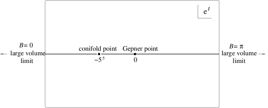
Figure 1: Kähler moduli space for a B-orientifold of the quintic

2.3.2 A Two parameter Model

In the example $(8,8,4,4,4)$, there is a unique non-trivial and involutive dressing by quantum symmetry. Also, there are several non-trivial and involutive dressing by the global symmetry ${\mathbb{Z}}_{8}\times{\mathbb{Z}}_{4}^{3}$. Here, since there are already a variety of ways to choose ${\bf m}$ for a fixed $\sigma$, we only consider the $\sigma={\rm id}$ cases.

For A-type parity, $X_{i}\rightarrow\,{\rm e}^{2\pi im_{i}\over k_{i}+2}\overline{X_{i}}$, ${\bf m}$ obey the equivalence relation $m_{i}\equiv m_{i}+2n_{i}$ and $m_{i}\equiv m_{i}+1$, and there are six independent choices ${\bf m}=(00000)$, $(00001)$, $(00011)$, $(00111)$, $(01000)$, $(01001)$. Under the quantum symmetry $g_{-1}$, the term $\widetilde{X}_{1}\cdots\widetilde{X}_{5}$ in the dual superpotential (2.12) flips its sign while $\widetilde{X}_{1}^{4}\widetilde{X}_{2}^{4}$ is invariant. Thus, if dressed by the quantum symmetry $g_{-1}$, the Kähler modulus $t=2t_{1}+t_{2}$ is frozen at $\,{\rm e}^{t}=0$ but $\,{\rm e}^{t_{2}}$ is unconstrained. If not dressed by quantum symmetry, the Kähler moduli are both unconstrained. In the regime $t_{1},t_{2}\gg 0$, one can talk about the geometry. $\tau_{\bf m}^{A}$ acts as an antiholomorphic involution, and the fixed point set is $X_{i}=\,{\rm e}^{\pi im_{i}\over k_{i}+2}x_{i}$, and $X_{6}=x_{6}$, where $x_{i}$ are all real, obey

$$(-1)^{m_{1}}x_{1}^{8}x_{6}^{4}+(-1)^{m_{2}}x_{2}^{8}x_{6}^{4}+(-1)^{m_{3}}x_{3}^{4}+(-1)^{m_{4}}x_{4}^{4}+(-1)^{m_{5}}x_{5}^{4}=0,$$

and are subject to the gauge conditions of the GLSM preserving the reality condition. The determination of the topology of the resulting fixed point sets can sometimes be a little cumbersome. This problem has been studied in [49] and we review here the parity $P^{A}_{00001}$ as an example. The topology of this O-plane can be obtained by studying the solutions of the real equation

$$x_{6}^{4}(x_{1}^{8}+x_{2}^{8})+x_{3}^{4}+x_{4}^{4}=x_{5}^{4}$$

subject to the rescaling

$$(x_{1},x_{2},x_{3},x_{4},x_{5},x_{6})\equiv(\lambda x_{1},\lambda x_{2},\mu x_{3},\mu x_{4},\mu x_{5},\lambda^{2}\mu x_{6})$$

with $\lambda,\mu\in{\mathbb{R}}^{*}$. Thus, we have to require $x_{5}\neq 0$, whereupon we can set $x_{5}$ to one by rescaling with $\mu$. The second rescaling can be absorbed by noting that $x_{1}^{8}+x_{2}^{8}>0$ in the large volume phase. After changing variables to $x_{1}^{8}=y_{1}^{2}$, $x_{2}^{8}=y_{2}^{2}$, $x_{6}^{4}=y_{6}^{2}$, $x_{3}^{4}=y_{3}^{2}$, $x_{4}^{4}=y_{4}^{2}$, the constraints become $y_{6}^{2}+y_{3}^{2}+y_{4}^{2}=1$, $y_{1}^{2}+y_{2}^{2}=1$, with non-trivial ${\mathbb{Z}}_{2}$ identification $(y_{1},y_{2},y_{3},y_{4},y_{6})\equiv(-y_{1},-y_{2},y_{3},y_{4},y_{6})$ (from $\lambda=-1$). Thus, topologically, this O-plane is $S^{2}\times{{\mathbb{R}}{\mathbb{P}}}^{1}=S^{2}\times S^{1}$.

We refer to [49] for the remaining cases, and summarize the results in Table 3. We do not know a simple description of the O-plane for the parity $P^{A}_{01001}$, except that it has Betti numbers $b_{0}=1$ and $b_{1}=2$. We have also indicated in table 3 that even though the number of moduli from complex structure deformations ($86$ real parameters) is always the same, each parity selects a different real section of the moduli space. In particular, these sections can intersect in different ways with singular loci, as we will illustrate below.

Table 3: A-type Orientifolds (with $\sigma=1$) of the Two Parameter Model

parity	moduli $(K,C)$	O-planes
$P^{A}_{+;00000}$	$(2_{{\mathbb{C}}},86_{{\mathbb{R}}})$	No O-plane
$P^{A}_{-;00000}$	$(1_{{\mathbb{C}}},86_{{\mathbb{R}}})$	non-geometric
$P^{A}_{+;00001}$	$(2_{{\mathbb{C}}},86_{{\mathbb{R}}}^{\prime})$	O6 at an $S^{2}\times S^{1}$
$P^{A}_{-;00001}$	$(1_{{\mathbb{C}}},86_{{\mathbb{R}}}^{\prime})$	non-geometric
$P^{A}_{+;00011}$	$(2_{{\mathbb{C}}},86_{{\mathbb{R}}}^{\prime\prime})$	O6 at a $T^{3}$
$P^{A}_{-;00011}$	$(1_{{\mathbb{C}}},86_{{\mathbb{R}}}^{\prime\prime})$	non-geometric
$P^{A}_{+;00111}$	$(2_{{\mathbb{C}}},86_{{\mathbb{R}}}^{\prime\prime\prime})$	O6 at an $S^{2}\times S^{1}$
$P^{A}_{-;00111}$	$(1_{{\mathbb{C}}},86_{{\mathbb{R}}}^{\prime\prime\prime})$	non-geometric
$P^{A}_{+;01000}$	$(2_{{\mathbb{C}}},86_{{\mathbb{R}}}^{\prime\prime\prime\prime})$	O6 at an $S^{3}$
$P^{A}_{-;01000}$	$(1_{{\mathbb{C}}},86_{{\mathbb{R}}}^{\prime\prime\prime\prime})$	non-geometric
$P^{A}_{+;01001}$	$(2_{{\mathbb{C}}},86_{{\mathbb{R}}}^{\prime\prime\prime\prime\prime})$	O6 at a SLAG with $b_{0}=1$, $b_{1}=2$
$P^{A}_{-;01001}$	$(1_{{\mathbb{C}}},86_{{\mathbb{R}}}^{\prime\prime\prime\prime\prime})$	non-geometric

For B-type parity, $X_{i}\rightarrow\,{\rm e}^{2\pi i(m_{i}+1/2)\over k_{i}+2}X_{i}$, ${\bf m}$ is constrained by $2m_{i}=0$ (mod $k_{i}+2$) and obey the equivalence relation $m_{i}\equiv m_{i}+1$. There are eight choices described by the signs $\epsilon_{i}=\,{\rm e}^{2\pi im_{i}\over k_{i}+2}$: $(\epsilon_{1}\epsilon_{2}\epsilon_{3}\epsilon_{4}\epsilon_{5})=(+++++)$, $(++-++)$, $(++--+)$, $(++---)$, $(+-+++)$, $(+--++)$, $(+---+)$, $(+----)$. If dressed with $g_{\omega}^{m}$ with $\omega=\,{\rm e}^{2\pi i/8}$, the monomials $\widetilde{X}_{1}\cdots\widetilde{X}_{5}$ and $\widetilde{X}_{1}^{4}\widetilde{X}_{2}^{4}$ of the dual variables are transformed to $\,{\rm e}^{2\pi im/8}\overline{\widetilde{X}_{1}\cdots\widetilde{X}_{5}}$ and $\,{\rm e}^{\pi im}\overline{\widetilde{X}_{1}^{4}\widetilde{X}_{2}^{4}}$ respectively. The symmetry condition $\widetilde{W}\rightarrow\overline{\widetilde{W}}$ is satisfied by the dual superpotential (2.12) if $\,{\rm e}^{2\pi im/8}\,{\rm e}^{t_{1}/4+t_{2}/8}=\overline{\,{\rm e}^{t_{1}/4+t_{2}/8}}$ and $\,{\rm e}^{\pi im}\,{\rm e}^{t_{2}/2}=\overline{\,{\rm e}^{t_{2}/2}}$. It follows from this that the Kähler moduli are constrained by

$$\mbox{not dressed by quantum symmetry:}\quad\,{\rm e}^{t_{1}}\in{\mathbb{R}},\quad\,{\rm e}^{t_{2}}\in{\mathbb{R}}_{\geq 0}\qquad$$ (2.19)

$$\mbox{dressed by odd quantum symmetry:}\quad\,{\rm e}^{t_{1}}\in{\mathbb{R}},\quad\,{\rm e}^{t_{2}}\in{\mathbb{R}}_{\leq 0},\qquad$$ (2.20)

Each of these have two large volume regions classified by the $B$-field. By using (2.10) and the charge table (2.7), one learns that in the case (2.19) the $B$-field can be $B=0$ or $B=\pi\omega_{1}$, while in the case (2.20), we have $B=\pi\omega_{2}$ or $B=\pi\omega_{1}+\pi\omega_{2}$.

To describe this real section of the moduli space of the two parameter model in somewhat more detail, we recall from [32] that by introducing

$$\xi=\,{\rm e}^{t_{2}+2t_{1}}\qquad\eta=\,{\rm e}^{t_{2}}\qquad\zeta=\,{\rm e}^{t_{1}+t_{2}}\,,$$

we can embed the parameter space as the quadric

$$Q=\{\xi\eta-\zeta^{2}=0\}$$ (2.21)

in ${\mathbb{C}}^{3}$. In these coordinates, the singularities in the parameter space of the mirror threefold (2.12) appear at the curves

$$C_{1} = Q\cap\{\eta=4\}$$ (2.22)

$$C_{\rm con} = Q\cap\{2^{-16}\xi+\eta-2^{-7}\zeta=4\}\,.$$ (2.23)

The real moduli space, $Q\cap\{\xi,\eta,\zeta\in{\mathbb{R}}\}$ is an ordinary double cone, which consist of the components $Q_{+}=Q\cap\{\xi,\eta>0\}$, and $Q_{-}=Q\cap\{\xi,\eta<0\}$, meeting at the tip $\xi=\eta=\zeta=0$ (Gepner point). In fact, from (2.19) and (2.20), we see that the real Kähler moduli space of the orientifold without (with) dressing by quantum symmetry is given by $Q_{+}$ ($Q_{-}$). Moreover, the real versions of $C_{1}$ and $C_{\rm con}$ are ordinary cone sections, and it is easy to check that they are parabolas and lie completely in $Q_{+}$. Since they intersect transversely and have co-dimension one, if we do not dress by quantum symmetry, the Gepner point is completely separated from the two large volume regimes. In that case, it is not possible to connect the Gepner point with a geometric interpretation of the orientifold without running into a singularity of the worldsheet theory. If dressed by odd quantum symmetry, the moduli space and singular loci do not meet, so that Gepner point is connected to the corresponding two large volume regimes.

In order to capture its global structure, it is convenient to compactify the moduli space by adding a divisor $C_{\infty}$ at infinity. As explained in [32], the compactification can be achieved by embedding $Q$ in (2.21) in the projective space ${\mathbb{P}}^{3}$, which by abuse of notation we coordinatize with $[\xi:\eta:\zeta:\tau]$. In addition to $C_{1}$ and $C_{\rm con}$, we then have the distinguished locus $C_{\infty}=Q\cap\{\tau=0\}$, which also corresponds to a degeneration of (2.12). We also have the “orbifold locus” $C_{0}=\{\xi=\zeta=0\}\subset Q$, which contains the Gepner point $g=[0:0:0:1]$. We show a picture of this compactified parameter space and the location of the singular loci $C_{0}$, $C_{1}$, $C_{\rm con}$, and $C_{\infty}$ in Figure 2. It is important to emphasize that in distinction to $C_{\rm con}$ and $C_{1}$, $C_{0}$ and $g$ do not lead to a singular worldsheet theory.

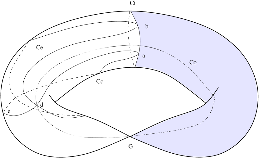
Figure 2: Real section of the Kähler moduli space of the two parameter model $(k_{i}+2)=(8,8,4,4,4)$. The Gepner point $g$ is at the tip of a conical singularity. The left cone is the moduli space of the orientifold without dressing by quantum symmetry. The lines of singularity $C_{1}$ and $C_{\rm con}$ divide the moduli space into several perturbative regions. The right cone (shaded region), which reaches out all the way to the large volume regime, is the moduli space of the orientifold with dressing by quantum symmetry.

Also, $C_{\infty}$ simply corresponds to the boundary of the uncompactified moduli space in the usual sense. In particular, the large volume limit has been hidden inside of $C_{\infty}$ by the compactification process. To recover this (unique) large volume limit, we need to blow up the point $b$, where the two divisors $C_{1}$ and $C_{\infty}$ intersect non transversely. Near $C_{\infty}$, we can work in the patch $\xi=1$ of ${\mathbb{P}}^{3}$, in which our real moduli space is given by the equation $\eta=\zeta^{2}$, with $\tau$ arbitrary. In this patch, $C_{1}$ is given by $\tau=\eta=\zeta^{2}$, while $C_{\infty}$ is given by $\tau=0$. A real blowup of the origin corresponds to replacing a small disc around $\zeta=\tau=0$ with a Möbius strip. The exceptional divisor (called $D_{(-1,-1)}$ in [32]) of this blowup is simply the non-trivial one-cycle of the Möbius strip. In simple terms, the blowup means that when approaching the origin along some path, we keep track of the first derivative $d\tau/d\zeta$, and we do not reach the same point depending on the value of this derivative. It is easy to see from this description that now $C_{1}$, $C_{\infty}$, and $D_{(-1,-1)}$ meet at a triple intersection, and we have to perform a second blowup, replacing the origin by the exceptional divisor $D_{(0,-1)}$. The large volume point is now the unique intersection point $D_{(0,-1)}\cap C_{\infty}$. In this way, we have recovered the description of the large volume limit as a cylinder $(t_{1},t_{2})\equiv(t_{1}+2\pi i,t_{2})\equiv(t_{1},t_{2}+2\pi i)$. We show this sequence of blowups in Figure 3.

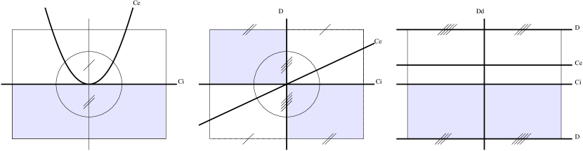
Figure 3: To see the large volume limit in the compactified moduli space, we have to blowup the singular point $b=C_{1}\cap C_{\infty}$. We replace twice a small neighborhood of the origin with a Möbius strip, successively inserting the divisors $D_{(-1,-1)}$ and $D_{(0,-1)}$. The multiply stroked lines are identified. The shaded region can be reached smoothly from the Gepner point.

This description puts us in a position to illustrate geometrically the statements on the structure of the large volume region that we have made above. The (real) neighborhood of the large volume point is divided by $D_{(0,-1)}$ and $C_{\infty}$ into four quadrants, which are geometrically distinguished by the value of the B-field. By following the sequence of blowups and the global picture in Figure 2, we see that starting from the Gepner point $g$, we can reach two of these quadrants without crossing a singularity, but not the other two.

We will use this description of the moduli space in section 7 when we discuss the comparison between Gepner model boundary and crosscap states and large volume.

Let us describe the topological structure of the orientifold planes corresponding to each of the involutions $\tau^{B}_{\epsilon}$ that we have defined above. In the large volume regime, $\tau^{B}_{\epsilon}$ acts on the manifold as the holomorphic involution $X_{i}\rightarrow\epsilon_{i}X_{i}$ and $X_{6}\rightarrow X_{6}$. The fixed point set is the loci with $\epsilon_{i}X_{i}=\lambda_{2}X_{i}$ ($i=1,2$), $\epsilon_{i}X_{i}=\lambda_{1}X_{i}$ ($i=3,4,5$), $X_{6}=\lambda_{1}\lambda_{2}^{-2}X_{6}$. The solutions in the eight cases are:
$(+++++)$:  No condition (the whole manifold $M$).
$(++-++)$:  $X_{3}=0$ (a hypersurface).
$(++--+)$:  $X_{3}=X_{4}=0$ (a curve of genus 9) and $X_{5}=X_{6}=0$ (four lines)
$(++---)$:  $X_{3}=X_{4}=X_{5}=0$ (eight points) and $X_{6}=0$ (a hypersurface).
$(+-+++)$:  $X_{1}=0$ or $X_{2}=0$ (two hypersurfaces). The two are homologous since they are two fibres of the K3-fibrations (with base $\{(X_{1},X_{2})\}$ and fibres $\{(X_{3},X_{4},X_{5},X_{6})\}$).
$(+--++)$:  $X_{1}=X_{3}=0$ or $X_{2}=X_{3}=0$ (two genus 3 curves). They are homologous to each other.
$(+---+)$:  $X_{1}=X_{5}=X_{6}=0$ (four points), $X_{1}=X_{3}=X_{4}=0$ (four points), $X_{2}=X_{5}=X_{6}=0$ (four points), $X_{2}=X_{3}=X_{4}=0$ (four points).
$(+----)$:  $X_{1}=X_{6}=0$ or $X_{2}=X_{6}=0$ (two genus 3 curves). They are homologous to each other.
These are included in Table 4.

Table 4: B-type Orientifolds (with $\sigma=1$) of the Two Parameter Model

parity	moduli $(K,C)$	O-planes
$P^{B}_{0;+++++}$	$(2_{{\mathbb{R}}},86_{{\mathbb{C}}},...,83_{{\mathbb{C}}})$	O9 at $M$
$P^{B}_{1;+++++}$	$(2^{\prime}_{{\mathbb{R}}},86_{{\mathbb{C}}})$
$P^{B}_{0;++-++}$	$(2_{{\mathbb{R}}},57_{{\mathbb{C}}},...,56_{{\mathbb{C}}})$	O7 at a hypersurface
$P^{B}_{1;++-++}$	$(2^{\prime}_{{\mathbb{R}}},57_{{\mathbb{C}}})$
$P^{B}_{0;++--+}$	$(2_{{\mathbb{R}}},46_{{\mathbb{C}}},...,47_{{\mathbb{C}}})$	O5’s at four rational and a genus 9 curves
$P^{B}_{1;++--+}$	$(2^{\prime}_{{\mathbb{R}}},46_{{\mathbb{C}}})$
$P^{B}_{0;++---}$	$(2_{{\mathbb{R}}},41_{{\mathbb{C}}},...,44_{{\mathbb{C}}})$	O7 at a hypersurface and O3’s at eight points
$P^{B}_{1;++---}$	$(2^{\prime}_{{\mathbb{R}}},41_{{\mathbb{C}}})$
$P^{B}_{0;+-+++}$	$(2_{{\mathbb{R}}},53_{{\mathbb{C}}},...,56_{{\mathbb{C}}})$	O7’s at two homologous K3 hypersurfaces
$P^{B}_{1;+-+++}$	$(2^{\prime}_{{\mathbb{R}}},53_{{\mathbb{C}}})$
$P^{B}_{0;+--++}$	$(2_{{\mathbb{R}}},46_{{\mathbb{C}}},...,47_{{\mathbb{C}}})$	O5’s at two homologous genus 3 curves
$P^{B}_{1;+--++}$	$(2^{\prime}_{{\mathbb{R}}},46_{{\mathbb{C}}})$
$P^{B}_{0;+---+}$	$(2_{{\mathbb{R}}},45_{{\mathbb{C}}},...,44_{{\mathbb{C}}})$	O3’s at sixteen points
$P^{B}_{1;+---+}$	$(2^{\prime}_{{\mathbb{R}}},45_{{\mathbb{C}}})$
$P^{B}_{0;+----}$	$(2_{{\mathbb{R}}},46_{{\mathbb{C}}},...,43_{{\mathbb{C}}})$	O5’s at two homologous genus 3 curves
$P^{B}_{1;+----}$	$(2^{\prime}_{{\mathbb{R}}},46_{{\mathbb{C}}})$

To conclude this section, we count the number of complex structure moduli in these orientifolds. This can be done by looking at the parity action on the corresponding chiral primary states. To see the action, we first consider the parities $P^{B}_{\omega;+++++}$ that correspond to the identity of $M$ in the large volume. In such a case, we know that the complex structure moduli is unconstrained. Thus the number of moduli is full $86$. Let us now go to the Gepner point along some path in the Kähler moduli space. As we have seen this can be done only for the parity $P^{B}_{1;+++++}$ dressed by an odd quantum symmetry. By continuity the number of moduli at the Gepner point is still $86$. Thus, we find that $P^{B}_{1;+++++}$ acts trivially on all the marginal $(c,c)$ primaries. Since other parities are obtained from $P^{B}_{1;+++++}$ by dressing global or quantum symmetries (whose action we know), we now know the action of all the parities $P^{B}_{\omega;{\bf m}}$ on the marginal $(c,c)$ primaries, at the Gepner point. In this way, we find the number of complex moduli at the Gepner point.
Remarks.
(i) By continuity the number of moduli found at the Gepner point applies everywhere in the Kähler moduli space for the parities $P^{B}_{1;\epsilon_{1}...\epsilon_{5}}$. This in particular tells us the number of moduli in the large volume limit. The numbers are listed in Table 4. (It is an interesting exercise to check these numbers directly by analyzing geometry.)
(ii) In the large volume regime, the only difference between $P_{1;\epsilon_{1}...\epsilon_{5}}$ and $P_{0;\epsilon_{1}...\epsilon_{5}}$ is the value of the $B$-field. Thus, the number found in (i) is still applicable for $P_{0;\epsilon_{1}...\epsilon_{5}}$, in the large volume regime.
(iii) On the other hand, one can analyze the action of $P_{0;\epsilon_{1}...\epsilon_{5}}$ at the Gepner point (as stated above). The action is the same as $P_{1;\epsilon_{1}...\epsilon_{5}}$ on the untwisted sector states but differs from that by $-$ sign on the twisted sector states. Thus, if $n$ twisted ground states survive the $P_{1;\epsilon_{1}...\epsilon_{5}}$-projection, then the other $(3-n)$ survive the $P_{0;\epsilon_{1}...\epsilon_{5}}$-projection.
(iv) Thus, the number of moduli is different between the Gepner point and the large volume regimes for the $P_{0,\epsilon_{1}...\epsilon_{5}}$-orientifolds. This is not a puzzle from the worldsheet point of view, because the two regions are separated by the singularity locus. There are also two other regions and the number of moduli there could be different as well. In Table 4, we only show the number at the large volume and at the Gepner point, and simply write dots … for the other two regions.

We have seen that the complex structure moduli can jump from from one component to another of the real Kähler moduli space. This tells us something about the full string theory. As we have discussed, the real Kähler moduli are combined with RR-potentials to form complex parameters (which become the lowest components of ${\mathcal{N}}=1$ chiral superfields of the spacetime theory). An interesting problem is to find the behaviour near the singularity. One possibility is that one can go around the singular loci by turning on the RR-potential, so that the separate regions of the real Kähler moduli space are smoothly connected to each other in the full moduli space (Figure 4(a)). This happens in other situations, such as the flop transition [37, 50].

Figure 4: Two possibilities of complexifying the real moduli space with a codimension one singularity. (a) One can go around the singularity and the two parts are smoothly connected. (b) The moduli space consists of branches. Any path from one region to the other must go through the singular point. Third possibility (not shown in Figure) would be that the two regions are disconnected.

This possibility is, however, eliminated in the present case by the jump in the dimension of the complex structure moduli space. One picture consistent with the jump is that the moduli space consists of a number of branches (Figure 4(b)), and the components of the real moduli space belong to different branches so that they can have different dimensions. Another possibility is that the singularity is at infinite distance and the two components are disconnected. Of course, the jump does not necessarily occur (an example is the case of quintic), and in such a case, at this stage we do not know whether one can go around the singular loci by turning on RR-potentials. It is an interesting problem to find out what is the right picture in full string theory.

3 Tadpole States of the Gepner Model

The main purpose of the present paper is to construct consistent Type II orientifolds on Calabi-Yau manifolds and Gepner models, with and without spacetime supersymmetry. In the discussion of consistency and spacetime supersymmetry, it is useful to study the “tadpole state” [51, 52], which is the sum of boundary and crosscap states:

$$|T\rangle=|B\rangle+|C\rangle=|B\rangle_{{}_{\rm NSNS}}+i|B\rangle_{{}_{\rm RR}}+i|C\rangle_{{}_{\rm NSNS}}+i|C\rangle_{{}_{\rm RR}}$$ (3.1)

and the “bra” version

$$\langle\theta T|=\langle\theta B_{\rm tot}|+\langle\theta C_{\rm tot}|={}_{{}_{\rm NSNS}}\!\langle B|+i{}_{{}_{\rm RR}}\!\langle B|-i{}_{{}_{\rm NSNS}}\!\langle C|+i{}_{{}_{\rm RR}}\!\langle C|.$$ (3.2)

The NSNS and RR parts are

$$\begin{array}[]{l}|B\rangle_{{}_{\rm NSNS}}=|B_{+}\rangle_{{}_{\rm NSNS}}-|B_{-}\rangle_{{}_{\rm NSNS}},\\ |B\rangle_{{}_{\rm RR}}=|B_{+}\rangle_{{}_{\rm RR}}-|B_{-}\rangle_{{}_{\rm RR}},\\ |C\rangle_{{}_{\rm NSNS}}=|C_{(-1)^{F_{R}}P}\rangle-|C_{(-1)^{F_{L}}P}\rangle,\\ |C\rangle_{{}_{\rm RR}}=|C_{P}\rangle-|C_{(-1)^{F}P}\rangle.\end{array}$$ (3.3)

Here $B_{+}$ and $B_{-}$ corresponds to the boundary conditions with the opposite spin structures, and $P$ is an involutive parity symmetry of the total system. Each term on the right hand sides of (3.3), say $|C_{P}\rangle$, can be written as the tensor product of the spacetime part and internal part:

$$|\mbox{spacetime}\rangle\otimes|\mbox{internal}\rangle.$$

The spacetime part is associated with the Neumann boundary condition (for boundary state) and the standard parity $\Omega$ (for the crosscap states), and is given by the standard coherent state of the $D$ free bosons/fermions, the ghost and the superghosts. The internal part depends on the detail of D-branes and orientifold.

In this section, we construct the internal part of the crosscap states corresponding to the orientifolds introduced in the previous section. We also reconstruct the rational boundary states of Gepner models from a perspective which is somewhat different from the one in the literature. The Cardy-PSS construction [6, 9] and its generalizations are usually formulated in the language of purely bosonic rational conformal field theories. In particular, in [11, 14, 12], formulas are developed for crosscaps and boundary states of rational conformal field theories with arbitrary simple-current modular invariants. The Gepner model, which is based on an $\mathcal{N}=2$ supersymmetric CFT, can in principle be formulated in this language, so that the general results are applicable. On the other hand, in [15], general results were derived on boundary and crosscap states in rational conformal field theories directly in the supersymmetric language, and using orbifold instead of simple-current techniques. In following this approach, we will find that it is a lot simpler.

3.1 Construction of the Crosscap States

The crosscap states of the Gepner model can be constructed as a straightforward application of the general method [15]. Let ${\mathcal{X}}$ be a bosonic conformal field theory with a finite abelian symmetry group $G$ with which one can define an orbifold ${\mathcal{X}}/G$. Suppose ${\mathcal{X}}$ has a parity symmetry $P$ that commutes with the $G$-projection operator $\sum_{g\in G}g/|G|$. Then, a parity symmetry is induced in the orbifold theory, which is denoted again by $P$, with the crosscap state

$$|\Scr{C}_{P}\rangle^{\rm orb}={1\over\sqrt{|G|}}\sum_{g\in G}|\Scr{C}_{gP}\rangle.$$ (3.4)

Here $|\Scr{C}_{gP}\rangle$ are the crosscap states for the parity symmetry $gP$ of ${\mathcal{X}}$, which are supposed to obey

$$\langle\Scr{C}_{gP}|q_{t}^{H}|\Scr{C}_{hP}\rangle={\rm Tr}\!\!\mathop{}_{{\mathcal{H}}_{gh^{-1}}}\Bigl{[}hPq_{l}^{H}\Bigr{]},\qquad\forall g,\,\forall h,$$ (3.5)

in which ${\mathcal{H}}_{gh^{-1}}$ is the space of states on the circle with $gh^{-1}$-twist. Indeed the Klein bottle amplitude

$${}^{\rm orb}\langle\Scr{C}_{P}|q_{t}^{H}|\Scr{C}_{P}\rangle^{\rm orb} = {1\over|G|}\sum_{g,h}\langle\Scr{C}_{gP}|q_{t}^{H}|\Scr{C}_{hP}\rangle={1\over|G|}\sum_{g,h}{\rm Tr}\!\!\mathop{}_{{\mathcal{H}}_{gh^{-1}}}\Bigl{[}hPq_{l}^{H}\Bigr{]}$$

$$= \sum_{g^{\prime}\in G}{\rm Tr}\!\!\mathop{}_{{\mathcal{H}}_{g^{\prime}}}\left[\Bigl{(}{1\over|G|}\sum_{h\in G}h\Bigr{)}Pq_{l}^{H}\right]$$

is the trace of $Pq_{l}^{H}$ over the space of states of the orbifold theory, ${\mathcal{H}}^{\rm orb}=\oplus_{g^{\prime}\in G}{\mathcal{H}}_{g^{\prime}}^{G}$. The crosscap state for the parity dressed with the quantum symmetry $g_{\omega}$ associated with a character $\omega:G\rightarrow U(1)$ is

$$|\Scr{C}_{g_{\omega}P}\rangle^{\rm orb}={1\over\sqrt{|G|}}\sum_{g\in G}\omega(g)^{-1}|\Scr{C}_{gP}\rangle.$$ (3.6)

If ${\mathcal{X}}$ has fermions, with mod 2 fermion number $(-1)^{F}$, the above story applies, with the condition (3.5) modified as

$$\langle\Scr{C}_{g(\pm)^{F}P}|q_{t}^{H}|\Scr{C}_{hP}\rangle={\rm Tr}\!\!\mathop{}_{{\mathcal{H}}_{(\mp 1)^{F}gh^{-1}}}\Bigl{[}(-1)^{F}hPq_{l}^{H}\Bigr{]},\qquad\forall g,\,\forall h.$$ (3.7)

Note that ${\mathcal{H}}_{(-1)^{F}}$ and ${\mathcal{H}}_{\rm id}$ are the NSNS and the RR sectors respectively.

In what follows, we apply this method to the Gepner model, which is the orbifold of the product of the minimal models $\prod_{i=1}^{r}M_{k_{i}}$ with respect to the group $\Gamma\cong{\mathbb{Z}}_{H}$.

3.1.1 A-type

We first consider A-parities of the Gepner model $P^{A}_{\omega;{\bf m}}=g_{\omega}\tau^{A}_{\bf m}\Omega_{A}$, where $\omega$ (an $H$-th root of unity) parametrizes the quantum symmetry and ${\bf m}=(m_{1},\ldots,m_{r})$ labels the $\prod_{i=1}^{r}{\mathbb{Z}}_{k_{i}+2}/{\mathbb{Z}}_{H}$ global symmetry. They are the ones induced from the parity symmetry of the product theory $\prod_{i=1}^{r}M_{k_{i}}$

$${\bf P}^{A}_{\bf m}=({\it g}^{m_{1}}P_{A},\ldots,{\it g}^{m_{r}}P_{A}),$$

where $P_{A}$ is the basic A-parity of the ${\mathcal{N}}=2$ minimal model associated with the transformation $X\rightarrow\overline{\Omega_{A}^{*}X}$ of the LG field. We note that ${\it g}P_{A}{\it g}^{-1}={\it g}^{2}P_{A}$.

The crosscap states for the A-parities ${\it g}^{m}P_{A}$ of the minimal model and their cousins $(-1)^{F}{\it g}^{m}P_{A}$, $(\pm 1)^{F}{\it g}^{m}\widetilde{P}_{A}$ (where $\widetilde{P}_{A}=\,{\rm e}^{-\pi iJ_{0}}P_{A}$) are obtained in [18] as follows

$$|\Scr{C}_{(\pm 1)^{F}{\it g}^{m}P_{A}}\rangle=|\Scr{C}_{2m-1,-1}(\pm)\rangle,$$ (3.8)

$$|\Scr{C}_{(\pm 1)^{F}{\it g}^{m}\widetilde{P}_{A}}\rangle=|\Scr{C}_{2m,0}(\mp)\rangle.$$ (3.9)

Here

$$|\Scr{C}_{n,s}(\pm)\rangle=\epsilon^{\pm}_{s}(-1)^{n-s\over 2}\left(\,{\sigma^{s}_{n,s}\over\sqrt{2}}|\Scr{C}_{n,s}\rangle\mp{\sigma^{s}_{n,s+2}\over\sqrt{2}}|\Scr{C}_{n,s+2}\rangle\,\right),$$ (3.10)

where

$$\sigma^{s}_{n,s^{\prime}}=\,{\rm e}^{\pi i\left(-{n^{2}\over 4(k+2)}+{s^{2}\over 8}\right)}\,{\rm e}^{-\pi ih_{0ns^{\prime}}},$$

$$\epsilon^{\pm}_{1}=\epsilon^{\pm}_{-1}=1,\qquad\epsilon^{\pm}_{0}=\epsilon^{\mp}_{2}=\,{\rm e}^{\pm{\pi i\over 4}},$$

and $|\Scr{C}_{n,s}\rangle$ are the PSS crosscaps of the GSO projected model ${SU(2)_{k}\times U(1)_{2}\over U(1)_{k+2}}$,

$$|\Scr{C}_{n,s}\rangle=\sum_{(l^{\prime}m^{\prime}s^{\prime})\in{\rm M}_{k}}{P_{0ns}^{\,\,\,\,l^{\prime}m^{\prime}s^{\prime}}\over\sqrt{S_{000}^{\,\,\,\,l^{\prime}m^{\prime}s^{\prime}}}}|\Scr{C},l^{\prime},m^{\prime},s^{\prime}\rangle\!\rangle.$$

In [18], the overall phase of these crosscaps are not determined. Here, we fix the phases as above, for the following reason.

The $n$-dependent part of the phase is important because this will affect the sum over the orbifold group elements, as in (3.4) or (3.6). The above choice is motivated by the transformation property under ${\it g}$ as well as the periodicity under $n\rightarrow n+2(k+2)$, as we now describe. One can show that the symmetry ${\it g}$ acts on these states as

$${\it g}:|\Scr{C}_{n,s}(\pm)\rangle\longmapsto|\Scr{C}_{n+4,s}(\pm)\rangle.$$ (3.11)

This is in accord with the fact that ${\it g}P_{A}{\it g}^{-1}={\it g}^{2}P_{A}$ and hence that ${\it g}|\Scr{C}_{\cdots{\it g}^{m}P_{A}}\rangle$ is proportional to $|\Scr{C}_{\cdots{\it g}^{m+2}P_{A}}\rangle$. What (3.11) means is that they are not just proportional but equal, under the identification (3.8)-(3.9) with the definition (3.10). Also note the periodicity

$$|\Scr{C}_{n+2(k+2),s}(\pm)\rangle=(-1)^{s}|\Scr{C}_{n,s}(\pm)\rangle.$$ (3.12)

The crosscap states that lie in the RR-sector have a double periodicity $n\equiv n+4(k+2)$. Thus, with the above choice of the $n$-dependence of the phase, these crosscaps corresponds precisely to the oriented O-planes in the LG model; $|\Scr{C}_{2m-1,-1}(\pm)\rangle$ corresponds to the O-plane at $X=\,{\rm e}^{\pi im\over k+2}x$, $x\in{\mathbb{R}}$, with the orientation that goes from positive $x$ to negative $x$. See Figure 5.

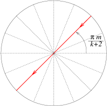
Figure 5: The O-plane corresponding to $|\Scr{C}_{2m-1,-1}(+)\rangle$. This is the example with $k+2=8$ and $m=2$.

As shown in [18], it has the right integral RR-charge: overlap with the RR-boundary states produces the correct results for the parity-twisted open string Witten indices — the intersection number.

The phase factor $\epsilon_{0}^{\pm}=\epsilon_{2}^{\mp}=\,{\rm e}^{\pm{\pi i\over 4}}$ is also added to the NSNS part of the crosscap state, in order to simplify the expression of the tension of the O-plane. In fact, we need the O-plane tension to be real in the end. Namely, we need the reality of the overlap of the crosscap with the NSNS ground state $|0\rangle_{{{}_{\rm NSNS}}}$, in the Gepner model. With the above choice, the overlap in the minimal model is

$${}_{{{}_{\rm NSNS}}}\langle 0|\Scr{C}_{2m,0}(\pm)\rangle=\left\{\begin{array}[]{ll}\sqrt{2\over(k+2)\sin({\pi\over k+2})}\cos\Bigl{(}{\pi\over 2(k+2)}\Bigr{)}&\mbox{$k$ odd},\\[5.69046pt] \sqrt{2\over(k+2)\sin({\pi\over k+2})}\exp\Bigl{(}\pm{(-1)^{m}\pi i\over 2(k+2)}\Bigr{)}&\mbox{$k$ even}.\end{array}\right.$$ (3.13)

If $k$ is odd, this is already real and is therefore the right choice. If $k$ is even, this is a non-trivial phase. However, as we will see, in the average over the orbifold group elements $\gamma^{\nu}$ ($\nu\in{\mathbb{Z}}_{H}$), the terms from even $\nu$ and the terms from odd $\nu$ have the opposite phase thanks to the $(-1)^{m}$ in (3.13), and the result of the average is real or pure imaginary depending on $\omega=1$ or $-1$. Thus, we will simply need to multiply $\omega^{1\over 2}=\pm 1$ or $\pm i$ in the final expression. (See Section 3.3.)

Applying the general method, we find that the crosscap states for $g_{\omega}P^{A}_{\bf m}=P^{A}_{\omega;{\bf m}}$ and their cousins (including $\widetilde{P}^{A}_{\omega;{\bf m}}=\,{\rm e}^{-\pi iJ_{0}}P^{A}_{\omega;{\bf m}}$) are given by

$$|\Scr{C}_{(\pm 1)^{F}P^{A}_{\omega;{\bf m}}}\rangle={1\over\sqrt{H}}\sum_{\nu=1}^{H}\omega^{-\nu}|\Scr{C}_{\gamma^{\nu}(\pm 1)^{F}{\bf P}^{A}_{\bf m}}\rangle^{\rm prod},$$ (3.14)

$$|\Scr{C}_{(\pm 1)^{F}\widetilde{P}^{A}_{\omega;{\bf m}}}\rangle={1\over\sqrt{H}}\sum_{\nu=1}^{H}\omega^{-\nu}|\Scr{C}_{\gamma^{\nu}(\pm 1)^{F}\widetilde{\bf P}^{A}_{\bf m}}\rangle^{\rm prod}.$$ (3.15)

in which

$$|\Scr{C}_{\gamma^{\nu}(\pm 1)^{F}{\bf P}^{A}_{\bf m}}\rangle^{\rm prod}=(-1)^{\sum_{i}{\nu\over k_{i}+2}}\bigotimes_{i=1}^{r}|\Scr{C}_{2m_{i}+2\nu-1,-1}(\pm)\rangle,$$ (3.16)

$$|\Scr{C}_{\gamma^{\nu}(\pm 1)^{F}\widetilde{\bf P}^{A}_{\bf m}}\rangle^{\rm prod}=\bigotimes_{i=1}^{r}|\Scr{C}_{2m_{i}+2\nu,0}(\mp)\rangle.$$ (3.17)

The sign factor $(-1)^{\sum_{i}{\nu\over k_{i}+2}}$ is introduced in the RR-crosscap, in order to maintain the periodicity under $\nu\rightarrow\nu+H$, which can be shown using (3.12). As mentioned above, we need to multiply the NSNS-part of the crosscap state $|\Scr{C}_{(\pm 1)^{F}\widetilde{P}^{A}_{\omega;{\bf m}}}\rangle$ by a phase $\omega^{1\over 2}$, in order for the O-plane tension to be real. This will be taken care of when we discuss the total crosscap state in string theory in the last subsection 3.3.

By the property (3.11) of each factor, we find the relation

$$\gamma^{\nu}|\Scr{C}_{{\bf P}^{A}}\rangle^{\rm prod}=|\Scr{C}_{\gamma^{2\nu}{\bf P}^{A}}\rangle^{\rm prod}$$ (3.18)

where ${\bf P}^{A}$ is one of $\gamma^{\nu^{\prime}}{\bf P}^{A}_{\bf m}$ or any of their cousins. This is in accord with the relation $\gamma^{2\nu}{\bf P}_{A}=\gamma^{\nu}{\bf P}^{A}\gamma^{-\nu}$. Using this property, we can rewrite the crosscap states in a useful way:
$H$ odd
If $H$ is odd, the set $\{\gamma^{\nu}{\bf P}^{A}\}_{\nu\in{\mathbb{Z}}_{H}}$ is the same as $\{\gamma^{2\nu}{\bf P}^{A}\}_{\nu\in{\mathbb{Z}}_{H}}$. Then, the crosscap state for the parity $P^{A}$ induced from ${\bf P}^{A}$ is simply

$$|\Scr{C}_{P^{A}}\rangle={1\over\sqrt{H}}\sum_{\nu=1}^{H}\gamma^{\nu}|\Scr{C}_{{\bf P}^{A}}\rangle^{\rm prod}.$$ (3.19)

This state is manifestly $\Gamma$-invariant. Note that there is no involutive dressing by quantum symmetry if $H$ is odd.
$H$ even
If $H$ is even, $\{\gamma^{\nu}{\bf P}^{A}\}_{\nu\in{\mathbb{Z}}_{H}}$ splits into the union of $\{\gamma^{2\nu}{\bf P}^{A}\}_{\nu\in{\mathbb{Z}}_{H/2}}$ and $\{\gamma^{2\nu+1}{\bf P}^{A}\}_{\nu\in{\mathbb{Z}}_{H/2}}$. The crosscap states for the parity $P^{A}$ or the one dressed by the involutive quantum symmetry $g_{-1}$ are given by

$$|\Scr{C}_{g_{\pm}P^{A}}\rangle={1\over\sqrt{H}}\sum_{\nu=1}^{H/2}\Biggl{\{}\gamma^{\nu}|\Scr{C}_{{\bf P}^{A}}\rangle^{\rm prod}\pm\gamma^{\nu}|\Scr{C}_{\gamma{\bf P}^{A}}\rangle^{\rm prod}\Biggr{\}},$$ (3.20)

which is also manifestly $\Gamma$-invariant.

3.1.2 B-type

The B-parities $P^{B}_{\omega;{\bf m}}$ of the Gepner model are the ones induced from the parity symmetry of the product theory

$${\bf P}_{\bf m}^{B}=({\it g}^{m_{1}}P_{B},\ldots,{\it g}^{m_{r}}P_{B}),$$

where $P_{B}$ is the basic B-parity of the minimal model associated with the transformation $X\rightarrow\,{\rm e}^{\pi i\over k+2}\Omega_{B}^{*}X$ of the LG field.

The crosscap states for the B-parities ${\it g}^{m}P_{B}$ of the minimal model and their cousins $(-1)^{F}{\it g}^{m}P_{B}$, $(\pm 1)^{F}{\it g}^{m}\widetilde{P}_{B}$ (where $\widetilde{P}_{B}=\,{\rm e}^{\pi iJ_{0}}P_{B}$) are obtained in [18] as follows

$$|\Scr{C}_{(\pm 1)^{F}{\it g}^{m}P_{B}}\rangle=|\Scr{C}^{B}_{m,1}(\pm)\rangle,$$ (3.21)

$$|\Scr{C}_{(\pm 1)^{F}{\it g}^{m}\widetilde{P}_{B}}\rangle=|\Scr{C}^{B}_{m,0}(\mp)\rangle.$$ (3.22)

Here, for $r\in{\mathbb{Z}}_{k+2}$ and $p\in\{0,1\}$

$$|\Scr{C}^{B}_{r,p}(\pm)\rangle={1\over\sqrt{k+2}}\sum_{\nu\in{\mathbb{Z}}_{k+2}}\,{\rm e}^{2\pi i{\nu(r+p/2)\over k+2}}V_{M}|\Scr{C}_{2\nu-p,-p}(\pm)\rangle$$ (3.23)

where $|\Scr{C}_{n,s}(\pm)\rangle$ is the A-type crosscap defined in (3.10) and $V_{M}$ is the mirror automorphism. More explicitly, $|\Scr{C}_{r,p}^{B}(\pm)\rangle=\epsilon^{B\pm}_{p}\,{\rm e}^{\pi ip{2r+p\over k+2}}\left({1\over\sqrt{2}}|\Scr{C}^{B}_{r0p}\rangle\pm{i\over\sqrt{2}}|\Scr{C}^{B}_{r1p}\rangle\right)$ in which $\epsilon_{1}^{B\pm}=\pm\,{\rm e}^{\mp{\pi i\over 4}}$, $\epsilon^{B\pm}_{0}=1$ and

$$|\Scr{C}_{rqp}^{B}\rangle:={1\over 2(k+2)}\sum_{n,s\atop{\rm even}}\,{\rm e}^{-\pi i\theta_{rq}(n,s)+\pi i\widehat{Q}_{(0pp)}(0ns)}V_{M}|\Scr{C}_{n+p.s+p}\rangle=\,{\rm e}^{-\pi ip{\widehat{2r+p}\over 2(k+2)}+\pi ip{\widehat{2q+p}\over 4}}|\Scr{C}_{rqp}\rangle^{\prime},$$

where

$$|\Scr{C}_{rqp}\rangle^{\prime}=(2(k+2))^{\frac{1}{4}}\sum_{j}\sigma_{j,2r+p,2q+p}\ \frac{P_{\frac{k}{2}j}}{\sqrt{S_{0j}}}(-1)^{\frac{\widehat{2r+p}-p}{2}+q}|\Scr{C},j,2r+p,2q+p\rangle\!\rangle_{B}$$

is the state denoted by $|\Scr{C}_{rqp}\rangle$ in [18].

Applying the general method, we find that the crosscap states for $(\pm 1)^{F}P^{B}_{\omega;{\bf m}}$ and $(\pm 1)^{F}\widetilde{P}^{B}_{\omega;{\bf m}}$ are

$$|\Scr{C}_{(\pm 1)^{F}P^{B}_{\omega;{\bf m}}}\rangle={1\over\sqrt{H}}\sum_{\nu=1}^{H}\omega^{-\nu}|\Scr{C}_{\gamma^{\nu}(\pm 1)^{F}{\bf P}^{B}_{\bf m}}\rangle^{\rm prod},$$ (3.24)

$$|\Scr{C}_{(\pm 1)^{F}\widetilde{P}^{B}_{\omega;{\bf m}}}\rangle={1\over\sqrt{H}}\sum_{\nu=1}^{H}\omega^{-\nu}|\Scr{C}_{\gamma^{\nu}(\pm 1)^{F}\widetilde{\bf P}^{B}_{\bf m}}\rangle^{\rm prod}.$$ (3.25)

in which

$$|\Scr{C}_{\gamma^{\nu}(\pm 1)^{F}{\bf P}^{B}_{\bf m}}\rangle^{\rm prod}=\bigotimes_{i=1}^{r}|\Scr{C}^{B}_{m_{i}+\nu,1}(\pm)\rangle,$$ (3.26)

$$|\Scr{C}_{\gamma^{\nu}(\pm 1)^{F}\widetilde{\bf P}^{B}_{\bf m}}\rangle^{\rm prod}=\bigotimes_{i=1}^{r}|\Scr{C}^{B}_{m_{i}+\nu,0}(\mp)\rangle.$$ (3.27)

Alternatively one could start with the A-type parities in the mirror Gepner model, which is the orbifold of the product of minimal models with the group $\widetilde{\Gamma}\subset\prod_{i}{\mathbb{Z}}_{k_{i}+2}$, $\widetilde{\nu}=(\widetilde{\nu}_{1},...,\widetilde{\nu}_{r})\in\widetilde{\Gamma}$ $\Leftrightarrow$ $\sum_{i=1}^{r}{\nu_{i}\over k_{i}+2}\in{\mathbb{Z}}$ (see Section 2.1.3). In the mirror system, the global symmetries are parametrized by ${\bf\widetilde{m}}=(\widetilde{m}_{1},...,\widetilde{m}_{r})\in\prod_{i}{\mathbb{Z}}_{k_{i}+2}$ modulo shift by $\widetilde{\nu}=(\widetilde{\nu}_{1},...,\widetilde{\nu}_{r})\in\widetilde{\Gamma}$, and the quantum symmetries are parametrized by $\widetilde{\omega}=(\widetilde{\omega}_{1},...,\widetilde{\omega}_{r})$, $\widetilde{\omega}_{i}^{k_{i}+2}=1$, modulo the relation $\widetilde{\omega}=\widetilde{\omega}^{\prime}$ $\Leftrightarrow$ $\prod_{i}(\widetilde{\omega}_{i}^{\prime}\widetilde{\omega}_{i}^{-1})^{\widetilde{\nu}_{i}}=1$ ($\forall\widetilde{\nu}\in\widetilde{\Gamma}$). They correspond respectively to the quantum symmetries $\omega$ and global symmetries ${\bf m}$ of the original Gepner model, under the map

$$\exp\left(-2\pi i{m_{i}\over k_{i}+2}\right)=\widetilde{\omega}_{i}.$$ (3.28)

$$\omega=\exp\left(2\pi i\sum_{i=1}^{r}{\widetilde{m}_{i}\over k_{i}+2}\right),$$ (3.29)

Then, the parity $P^{B}_{\omega;{\bf m}}$ of the Gepner model corresponds to the parity $P^{A}_{{\widetilde{\omega}};{\bf\widetilde{m}}}$ of the mirror Gepner model, whose crosscap states are given by

$$|\Scr{C}_{(\pm 1)^{F}P^{A}_{\widetilde{\omega};{\bf\widetilde{m}}}}\rangle={1\over\sqrt{|\widetilde{\Gamma}|}}\sum_{\widetilde{\nu}\in\widetilde{\Gamma}}\widetilde{\omega}^{-\widetilde{\nu}}(-1)^{\sum_{i}{\widetilde{\nu}_{i}\over k_{i}+2}}\bigotimes_{i=1}^{r}|\Scr{C}_{2\widetilde{m}_{i}+2\widetilde{\nu}_{i}-1,-1}(\pm)\rangle$$ (3.30)

$$|\Scr{C}_{(\pm 1)^{F}\widetilde{P}^{A}_{\widetilde{\omega};{\bf\widetilde{m}}}}\rangle={1\over\sqrt{|\widetilde{\Gamma}|}}\sum_{\widetilde{\nu}\in\widetilde{\Gamma}}\widetilde{\omega}^{-\widetilde{\nu}}\bigotimes_{i=1}^{r}|\Scr{C}_{2\widetilde{m}_{i}+2\widetilde{\nu}_{i},0}(\mp)\rangle,$$ (3.31)

where $\widetilde{\omega}^{-\widetilde{\nu}}$ is the short-hand notation for $\prod_{i}\widetilde{\omega}_{i}^{-\widetilde{\nu}_{i}}$. It is straightforward to show that

$$|\Scr{C}_{(\pm 1)^{F}P^{B}_{\omega;{\bf m}}}\rangle=\widetilde{\omega}^{-\bf\widetilde{m}}\,{\rm e}^{\pi i\sum_{i}{\widetilde{m}_{i}\over k_{i}+2}}V_{M}|\Scr{C}_{(\pm 1)^{F}P^{A}_{\widetilde{\omega};{\bf\widetilde{m}}}}\rangle$$ (3.32)

$$|\Scr{C}_{(\pm 1)^{F}\widetilde{P}^{B}_{\omega;{\bf m}}}\rangle=\widetilde{\omega}^{-\bf\widetilde{m}}V_{M}|\Scr{C}_{(\pm 1)^{F}\widetilde{P}^{A}_{\widetilde{\omega};{\bf\widetilde{m}}}}\rangle$$ (3.33)

The two sets of crosscap states differ by phases. Actually, by the condition that $P^{B}_{\omega;{\bf m}}$ is involutive, $m_{i}$ must be $0$ or $(k_{i}+2)/2$, or $\widetilde{\omega}_{i}=\pm 1$. Thus the overall factor $\widetilde{\omega}^{-{\bf\widetilde{m}}}$ common to all the four states is just a sign. On the other hand, the factor $\,{\rm e}^{\pi i\sum_{i}{\widetilde{m}_{i}\over k_{i}+2}}$ is a non-trivial phase that makes a real difference. It turns out that the one obtained from the mirror theory is the right choice. This can be understood by noting that the parity twisted Witten indices for open strings is automatically integral in the A-type crosscaps. Thus, we modify the RR part of the crosscap in the original construction as

$$(\ref{CGB1})\longrightarrow\qquad|\Scr{C}_{(\pm 1)^{F}P^{B}_{\omega;{\bf m}}}\rangle={1\over\sqrt{H}}\sum_{\nu=1}^{H}\omega^{-\nu-{1\over 2}}|\Scr{C}_{\gamma^{\nu}(\pm 1)^{F}{\bf P}^{B}_{\bf m}}\rangle^{\rm prod},\qquad$$ (3.34)

where $\omega^{-{1\over 2}}$ is identified as $\,{\rm e}^{-\pi i\sum_{i}{\widetilde{m}_{i}\over k_{i}+2}}$.

3.2 Boundary States

The construction of the boundary states is likewise a straightforward application of the general method. Let ${\mathcal{X}}$ and $G$ be as in the beginning of the previous subsection. We are interested in constructing a D-brane boundary state in ${\mathcal{X}}/G$ from a D-brane $\Scr{B}$ of ${\mathcal{X}}$. If $\Scr{B}$ is not invariant under any element of $G$, $\Scr{B}\mapsto g\Scr{B}\neq\Scr{B}$ ($g\neq 1$), the boundary state is simply the sum over the images

$$|\Scr{B}\rangle^{\rm orb}={1\over\sqrt{|G|}}\sum_{g\in G}g|\Scr{B}\rangle.$$ (3.35)

If $\Scr{B}$ is invariant under a subgroup $H$ of $G$, the boundary states is the sum over images $g\Scr{B}$ ($g\in G/H$) as well as the twist $h\in H$

$$|\Scr{B}\rangle^{\rm orb}={1\over\sqrt{|G|}}\sum_{g\in G/H\atop h\in H}g|\Scr{B}\rangle_{h}.$$ (3.36)

Here $|\Scr{B}\rangle_{h}$ is the boundary state for $\Scr{B}$ on the $h$-twisted circle. They are assumed to obey the relation

$${}_{h}\!\langle\Scr{B}|q_{t}^{H}g|\Scr{B}\rangle_{h}={\rm Tr}\!\!\mathop{}_{{\mathcal{H}}_{\Scr{B},g\Scr{B}}}\left[hq_{l}^{H}\right]$$

where ${\mathcal{H}}_{\Scr{B},g\Scr{B}}$ is the space of $\Scr{B}$-$g\Scr{B}$ open string states. Indeed the cylinder amplitude

$${}^{\rm orb}\!\langle\Scr{B}|q_{t}^{H}|\Scr{B}\rangle^{\rm orb} = {1\over|G|}\sum_{g_{1},g_{2}\in G/H\atop h\in H}{}_{h}\!\langle\Scr{B}|g_{1}^{-1}q_{t}^{H}g_{2}|\Scr{B}\rangle_{h}={1\over|H|}\sum_{g\in G/H\atop h\in H}{}_{h}\!\langle\Scr{B}|q_{t}^{H}g|\Scr{B}\rangle_{h}$$

$$= \sum_{g\in G/H}{\rm Tr}\!\!\mathop{}_{{\mathcal{H}}_{\Scr{B},g\Scr{B}}}\left[\left({1\over|H|}\sum_{h\in H}h\right)q^{H}\right]$$

is the sum over all possible pairs $\Scr{B}$-$g\Scr{B}$ of the trace over the $H$-invariant open string states. If we modify the action of $H$ on the Chan-Paton factor, we obtain a different brane. The brane associated with the proper $H$-action given by an $H$-character $h\mapsto\psi(h)\in U(1)$ has the boundary state

$$|\Scr{B}^{\psi}\rangle^{\rm orb}={1\over\sqrt{|G|}}\sum_{g\in G/H\atop h\in H}\psi(h)g|\Scr{B}\rangle_{h}.$$ (3.37)

One may also want to include the effects of discrete torsion. As argued in [53], this corresponds to having a projective representation of the orbifold group on the space of open string states. At the level of boundary states, one uses the alternating bihomomorphism $\epsilon:H\times H\longrightarrow U(1)$ obtained from the discrete torsion to define a subgroup $K$ of $H$ for each $G$-orbit of branes as

$$K=\{k\in H;\epsilon(k,h)=1\;\forall h\in H\}\,.$$ (3.38)

One obtains one elementary brane in the orbifold theory for each character $k\mapsto\psi(k)\in U(1)$ of $K$. The corresponding boundary state is a slight modification of (3.37)

$$|\Scr{B}^{\psi}\rangle^{\rm orb}={1\over\sqrt{|G|}}\sqrt{\frac{|H|}{|K|}}\sum_{g\in G/H\atop h\in H}\psi(h)g|\Scr{B}\rangle_{h},$$ (3.39)

where the extension of $\psi$ to $H\setminus K$ is irrelevant. We note that by general properties of group cohomology, the factor $\sqrt{|H|/|K|}$ is always integer.

Rational boundary states of the Gepner model can be obtained as an application of the methods described above. A-branes in the product theory are generically not invariant under any element of the orbifold group (the case $H=\{{\rm id}\}$) and thus the boundary states in the orbifold model are simply the sum over images. This is how these states were first written down in [7]. B-branes of the product theory, on the other hand, are all $\Gamma$-invariant (the case $H=G$) and therefore the boundary states are simply the sum over $\Gamma$-twists. This way of obtaining the B-type boundary states appears to be new, but we have found it to to be equivalent to the procedure developed in [7, 12, 24]. In particular, as we will see, the fixed point resolution prescription of [24] is correctly reproduced.

3.2.1 A-Branes

A-branes in the minimal model are denoted as $\Scr{B}^{A}_{L,M,S}$ and are labeled by $(L,M,S)\in{\rm M}_{k}$. Shift of $S$-label by $2$ is simply the orientation change — the sign flip of RR boundary states. $\Scr{B}^{A}_{L,M,S}$ preserve the combination $\overline{G}_{+}-(-1)^{S}G_{-}$ of the $(2,2)$ superconformal symmetry. The symmetry ${\it g}$ shifts the $M$-label by $2$. The boundary states on the NSNS and RR sectors are given by

$$|\Scr{B}_{L,M}^{A}\rangle_{{}_{\rm NSNS}}={1\over\sqrt{2}}|\Scr{B}_{L,M,S}\rangle+{1\over\sqrt{2}}|\Scr{B}_{L,M,S+2}\rangle,$$

$$|\Scr{B}_{L,M,S}^{A}\rangle_{{}_{\rm RR}}={1\over\sqrt{2}}|\Scr{B}_{L,M,S}\rangle-{1\over\sqrt{2}}|\Scr{B}_{L,M,S+2}\rangle,$$

where $|\Scr{B}_{L,M,S}\rangle$ are the standard Cardy brane of the GSO projected model ${SU(2)_{k}\times U(1)_{2}\over U(1)_{k+2}}$:

$$|\Scr{B}_{L,M,S}\rangle=\sum_{(lms)\in{\rm M}_{k}}{S_{LMS}^{\,\,\,\,lms}\over\sqrt{S_{000}^{\,\,\,\,lms}}}|l,m,s\rangle\!\rangle.$$

In the LG model, they correspond to the D1-brane at the wedge-shaped lines cornering at $X=0$. The wedge corresponding to $\Scr{B}_{L,M,S=1}^{A}$ is coming in from the direction $\arg(X)={\pi(M-L-1)\over k+2}$ and going out to the direction $\arg(X)={\pi(M+L+1)\over k+2}$. Replacing $S=1$ by $S=-1$ flips the orientation. See Figure 6.

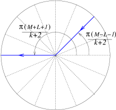
Figure 6: The A-brane $\Scr{B}^{A}_{L,M,S}$. This is the example $(L,M,S)=(2,5,1)$ for $k+2=8$.

We are interested in the D-brane of the Gepner model corresponding to the product brane

$$\Scr{B}^{A}_{{\bf L,M},S}=\Scr{B}^{A}_{L_{1},M_{1},S_{1}}\times\cdots\times\Scr{B}^{A}_{L_{r},M_{r},S_{r}}.$$

We need $S_{i}$ all even or all odd (i.e. $L_{i}+M_{i}$ all even or all odd), so that either one of $\overline{G}_{+}\mp G_{-}$ is preserved. Orientation flip of even number of factors does not change the total orientation. Thus the brane depends only on the total orientation $S=[{\bf S}]$ where $[{\bf S}]\equiv[{\bf S}^{\prime}]$ if the number of factors with $S_{i}^{\prime}=S_{i}+2$ is even. (If $r$ is odd, $S$ can be realized as the sum $S=\sum_{i}S_{i}\in{\mathbb{Z}}_{4}$.) The orbifold group element $\gamma^{\nu}$ sends $\Scr{B}^{A}_{{\bf L,M},S}$ to $\Scr{B}^{A}_{{\bf L,M+2\nu},S}$ (where ${\bf 2\nu}=(2\nu,2\nu,...,2\nu)$). Thus generically, $\Scr{B}^{A}_{{\bf L,M},S}$ is not invariant under any element of the orbifold group. Then, the boundary state is simply the sum over images

$$|\Scr{B}^{A}_{\bf L,M}\rangle_{{{}_{\rm NSNS}}}={1\over\sqrt{H}}\sum_{\nu=1}^{H}\bigotimes_{i=1}^{r}|\Scr{B}^{A}_{L_{i},M_{i}+2\nu}\rangle_{{{}_{\rm NSNS}}}$$ (3.40)

$$|\Scr{B}^{A}_{{\bf L,M},S}\rangle_{{{}_{\rm RR}}}={1\over\sqrt{H}}\sum_{\nu=1}^{H}\bigotimes_{i=1}^{r}|\Scr{B}^{A}_{L_{i},M_{i}+2\nu,S_{i}}\rangle_{{{}_{\rm RR}}}.$$ (3.41)

It is a simple exercise to show that, adding the transverse modes of the spacetime and imposing chiral GSO projection, these lead to the boundary states obtained by Recknagel and Schomerus [7].

The construction is different if the product brane is invariant under a non-trivial orbifold group element, $\Scr{B}^{A}_{{\bf L,M+2\nu},S}=\Scr{B}^{A}_{{\bf L,M},S}$, see [22, 23]. Branes of different $M$ labels can be the same because of the “Field Identification” (FI) $(L,M,S)=(k-L,M+k+2,S+2)$. Since FI is involutive we find that $2\nu=0$ mod $H$. Thus, the stabilizer group is at most the ${\mathbb{Z}}_{2}$ subgroup generated by $\gamma^{H\over 2}$, which is possible only when $H$ is even. Under the symmetry $\gamma^{H/2}$, the brane $\Scr{B}^{A}_{{\bf L,M},S}$ transforms to $\Scr{B}^{A}_{{\bf L,M+{(k+2)}{{\it H}\over k+2}},S}$. For the factor $i$ such that $w_{i}={H\over k_{i}+2}$ is even, the brane remains the same because $\Scr{B}_{L_{i},M_{i}+2(k_{i}+2),S_{i}}=\Scr{B}_{L_{i},M_{i},S_{i}}$. For the factor $i$ such that $w_{i}$ is odd, the brane $\Scr{B}_{L_{i},M_{i},S_{i}}$ is transformed to $\Scr{B}_{L_{i},M_{i}+k_{i}+2,S_{i}}$. In the LG picture, $M_{i}\rightarrow M_{i}+k_{i}+2$ is rotation by $\pi$, under which a “straight-wedge brane” ($L_{i}={k_{i}\over 2}$) is mapped to itself with an orientation flip. See Fig. 7.

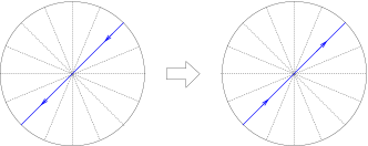
Figure 7: 180^∘ rotation reverses the orientation of the “straight-wedge” branes.

Note that there are even number of $i$’s such that $w_{i}$ is odd. (Remark (ii) in Section 2.1.) The total orientation is preserved even if the orientation is reserved for each of such $i$. Thus, the brane $\Scr{B}^{A}_{{\bf L,M},S}$ is invariant under $\gamma^{H/2}$ if and only if $L_{i}={k_{i}\over 2}$ for such $i$ that $w_{i}$ is odd. The boundary state is obtained as the application of the general formula (3.37):

$$|\widehat{\Scr{B}}^{(\pm)\,A}_{{\bf L,M}}\rangle_{{{}_{\rm NSNS}}}={1\over\sqrt{H}}\sum_{\nu=1}^{H\over 2}\gamma^{\nu}|\Scr{B}^{A}_{{\bf L,M}}\rangle^{\rm prod}_{{{}_{\rm NSNS}}}\pm{1\over\sqrt{H}}\sum_{\nu=1}^{H\over 2}\gamma^{\nu}|\Scr{B}^{A}_{{\bf L,M}}\rangle^{\rm prod}_{(-1)^{F}\gamma^{H/2}},$$ (3.42)

$$|\widehat{\Scr{B}}^{(\pm)\,A}_{{\bf L,M},S}\rangle_{{{}_{\rm RR}}}={1\over\sqrt{H}}\sum_{\nu=1}^{H\over 2}\gamma^{\nu}|\Scr{B}^{A}_{{\bf L,M},S}\rangle^{\rm prod}_{{{}_{\rm RR}}}\pm{1\over\sqrt{H}}\sum_{\nu=1}^{H\over 2}\gamma^{\nu}|\Scr{B}^{A}_{{\bf L,M},S}\rangle^{\rm prod}_{\gamma^{H/2}},$$ (3.43)

Note that the untwisted part is simply one half of (3.40) or (3.41). The boundary state $|\Scr{B}_{{\bf L,M},S}\rangle^{\rm prod}_{(\mp 1)^{F}\gamma^{H/2}}$ is given by the product of the twisted states $|\Scr{B}_{L_{i},M_{i},S_{i}}\rangle_{(\mp 1)^{F}\tilde{{\it g}}^{H/2}}$ of the minimal model. Here we replaced ${\it g}$ by $\tilde{{\it g}}$ where $\tilde{{\it g}}=g$ if $w_{i}$ is even while $\tilde{g}=a^{2}=\,{\rm e}^{-2\pi iJ_{0}}={\it g}(-1)^{\widehat{F}}$ if $w_{i}$ is odd. This is because $a^{k_{i}+2}$ preserves the $L_{i}={k_{i}\over 2}$ branes including the orientation. (Since there are even number of $i$’s with odd $w_{i}$, this makes no difference.) The twist $\tilde{{\it g}}^{H/2}$ is trivial for such $i$ that $w_{i}$ is even, while it is non-trivial, $\tilde{{\it g}}^{H/2}=a^{k_{i}+2}$, for such $i$ that $w_{i}$ is odd. The $a^{k+2}$-twisted boundary state in the minimal model is given by

$$|\Scr{B}_{{k\over 2},M,S}^{A}\rangle_{(\mp 1)^{F}a^{k+2}}=\sum_{{k\over 2}+m+s\,{\rm even}\atop s\,{\rm even/odd}}\,{\rm e}^{\pi i\left(-{M+S^{2}+Ss+m\over 2}+{Mm+m\over k+2}\right)}|{k\over 2},m,s\rangle\!\rangle.$$ (3.44)

Since the length of the sum over images is one half of the ordinary branes, these branes are called short orbit branes. “Field Identification” is a little different on these short orbit branes. $(L_{i},M_{i},S_{i})\rightarrow(k_{i}-L_{i},M_{i}+k_{i}+2,S_{i}+2)$ does not change the brane if $w_{i}$ is even, but exchanges $+$ and $-$ label if we do this for odd number of $i$’s with odd $w_{i}$.

3.2.2 B-Branes

B-branes in the minimal model can be obtained as the mirror of the A-branes in the ${\mathbb{Z}}_{k+2}$-orbifold model, see [7, 24, 26, 15]. (They can also be obtained directly as an application of the methods of [14] by using the results of [49] on the ${\mathbb{Z}}_{2}$ orbifold of the minimal models by mirror symmetry automorphism.) The mirror of the brane associated with $\Scr{B}^{A}_{L,M,S}$ is denoted as $\Scr{B}^{B}_{L,M,S}$ and they preserve the combination $G_{+}-(-1)^{S}G_{-}$ of the worldsheet superconformal symmetry. They are invariant under the symmetry ${\it g}$, and the boundary states on the various twisted circles are given by

$$|\Scr{B}_{L,M,S}^{B}\rangle_{(-1)^{(s^{\prime}+1)F}{\it g}^{n^{\prime}}} = {1\over\sqrt{k+2}}V_{M}\sum_{\widetilde{\nu}\in{\mathbb{Z}}_{k+2}}\,{\rm e}^{2\pi i{\widetilde{\nu}n^{\prime}\over k+2}}|\Scr{B}^{A}_{L,M+2\widetilde{\nu},S}\rangle_{(-1)^{(s^{\prime}+1)F}}$$

$$= (2k+4)^{{1\over 4}}\,{\rm e}^{-\pi i{Mn^{\prime}\over k+2}+\pi i{Ss^{\prime}\over 2}}\sum_{l^{\prime}\in{\rm P}_{k}\atop\nu_{1}\in{\mathbb{Z}}_{2}}{S_{Ll^{\prime}}\over\sqrt{S_{0l^{\prime}}}}(-1)^{S\nu_{1}}|l^{\prime},n^{\prime},s^{\prime}+2\nu_{1}\rangle\!\rangle_{B},$$

where $s^{\prime}=0$ for NSNS sector and $s^{\prime}=1$ for RR sector. Note that the $M$-label appears only on the overall phase for the boundary state with a non-trivial twist $g^{n^{\prime}}\neq 1$. Thus, the brane themselves depend only on $(L,S)$ but the $M$-label parametrizes the action of the global symmetry ${\it g}$ on the Chan-Paton factor. There is no short orbit branes in the naïve sense, since none of the A-branes is invariant under any non-trivial element of ${\mathbb{Z}}_{k+2}$. However, in the GSO projected model (i.e. in the coset model), B-branes are realized as the mirror of the A-branes in the ${\mathbb{Z}}_{k+2}\times{\mathbb{Z}}_{2}$ orbifold, and for even $k$ the Cardy branes $\Scr{B}_{{k\over 2},M,S}$ are invariant under the ${\mathbb{Z}}_{2}$ subgroup generated by $g_{k+2,2}$. Thus, there are short-orbit branes in the coset model, and resolving the GSO projection we obtain short orbit branes $\widehat{\Scr{B}}_{{k\over 2},M,S}^{B}$ in the minimal model. They are invariant under the symmetry $a^{2}=\,{\rm e}^{-2\pi iJ_{0}}={\it g}(-1)^{\widehat{F}}$. The boundary states on the various twisted circles are [18]

$$\!\!\!\!|\widehat{\Scr{B}}_{{k\over 2},M,S}^{B}\rangle_{(-1)^{(n^{\prime}+1)F}a^{2n^{\prime}}}={1\over\sqrt{2}}|\Scr{B}^{B}_{{k\over 2},M,S}\rangle_{(-1)^{(n^{\prime}+1)F}g^{n^{\prime}}}$$

$$\!\!\!\!|\widehat{\Scr{B}}_{{k\over 2},M,S}^{B}\rangle_{(-1)^{n^{\prime}F}a^{2n^{\prime}}}=\,{\rm e}^{-\pi i{Mn^{\prime}+n^{\prime}\over k+2}+\pi i{Sn^{\prime}+n^{\prime}\over 2}}\sqrt{k+2\over 2}\sum_{s=\pm 1}\,{\rm e}^{-\pi i{S(S-s)\over 2}}|{k\over 2},{k+2\over 2}+n^{\prime},s+n^{\prime}\rangle\!\rangle_{B}.$$

The long orbit brane $\Scr{B}^{B}_{L,M,1}$ is described in the LG model $W=X^{k+2}$ as the one associated with the boundary superpotential

$$V={\mit\Gamma}X^{L+1}$$

where ${\mit\Gamma}$ is a fermionic chiral superfield on the boundary with constraint $\overline{D}{\mit\Gamma}=X^{k+1-L}$ and $M$ labels the action of ${\it g}:X\rightarrow\,{\rm e}^{2\pi i\over k+2}X$ on the Chan-Paton ground state $|0\rangle$ (annihilated by the lowest component of ${\mit\Gamma}$) as

$${\it g}:|0\rangle\longmapsto\,{\rm e}^{-{2\pi i\over k+2}{M+L+1\over 2}}|0\rangle.$$

On the other hand, short orbit branes are not realized in the LG model with $W=X^{k+2}$ but in the model with $W=X^{k+2}-Y^{2}$ that also flows to the ${\mathcal{N}}=2$ minimal model. They are associated with the boundary superpotential

$$V={\mit\Gamma}(X^{k+2\over 2}-Y),\qquad\overline{D}{\mit\Gamma}=X^{k+2\over 2}+Y.$$

In the open string stretched between long and short orbit branes, there are odd number of real fermionic zero modes [18]. This imposes a strong constraint in the construction of consistent set of D-branes.

Let us first consider the product of long-orbit branes

$$\Scr{B}^{B}_{{\bf L},M,S}=\Scr{B}^{B}_{L_{1},M_{1},S_{1}}\times\cdots\times\Scr{B}^{B}_{L_{r},M_{r},S_{r}}.$$

$S_{i}$ are all even or all odd and the brane depends only on the total orientation $S=[{\bf S}]$. Also, the $\Gamma$ action on the Chan-Paton factor depends only on

$$M:=H\sum_{i=1}^{r}{M_{i}\over k_{i}+2}\in{\mathbb{Z}}_{2H}$$ (3.46)

which is even or odd depending on whether $\sum_{i}L_{i}H/(k_{i}+2)+HrS_{i}$ is even or odd. The choice of $M$ corresponds to the choice of representation of $\Gamma$ on the Chan-Paton factor.
The brane $\Scr{B}^{B}_{{\bf L},M,S}$ is invariant under all element of the orbifold group. Thus, the boundary state in the orbifold theory is simply the sum over the twists.

$$|\Scr{B}^{B}_{{\bf L},M,S}\rangle_{(-1)^{(s^{\prime}+1)F}}={1\over\sqrt{H}}\sum_{\nu\in{\mathbb{Z}}_{H}}\bigotimes_{i=1}^{r}|\Scr{B}^{B}_{L_{i},M_{i},S_{i}}\rangle_{(-1)^{(s^{\prime}+1)F}g^{\nu}}$$

$$= {1\over\sqrt{H}}\sum_{\nu\in{\mathbb{Z}}_{H}\atop\nu_{i}\in{\mathbb{Z}}_{2}^{r},l_{i}^{\prime}\in{\rm P}_{k_{i}}}\otimes_{i}(2k_{i}+2)^{1\over 4}\,{\rm e}^{-\pi i{M_{i}\nu\over k_{i}+2}+\pi i{S(s^{\prime}+2\nu_{i})\over 2}}{S_{L_{i}l_{i}^{\prime}}\over{\sqrt{S_{0l_{i}^{\prime}}}}}|l_{i}^{\prime},\nu,s^{\prime}+2\nu_{i}\rangle\!\rangle_{B},$$

where $s^{\prime}=0$ for NSNS and $s^{\prime}=1$ for RR. This B-brane can be identified as the A-brane in the mirror Gepner model associated with the product $\Scr{B}_{L_{1},M_{1},S_{1}}\times\cdots\times\Scr{B}_{L_{r},M_{r},S_{r}}$. It is a simple exercise to reproduce the above boundary states from this point of view. This realization will be useful in the discussion of the tadpole cancellation.

Next let us consider the brane involving short-orbit branes of the minimal model. There is one important constraint: the number of minimal model factors having short-orbit branes must be even. This is to avoid the open strings to have odd number of real fermionic zero modes, which would be problematic upon quantization. Thus, we will only consider product branes with even number of $\widehat{\Scr{B}}^{B}_{{k_{i}\over 2},M_{i},S_{i}}$ such as

$$\widehat{\Scr{B}}_{{\bf L},M,S}=\widehat{\Scr{B}}^{B}_{{k_{1}\over 2},M_{1},S_{1}}\times\widehat{\Scr{B}}^{B}_{{k_{2}\over 2},M_{2},S_{2}}\times\Scr{B}^{B}_{L_{3},M_{3},S_{3}}\times\cdots\times\Scr{B}^{B}_{L_{r},M_{r},S_{r}}.$$

The global symmetry ${\it g}$ preserves the long-orbit brane but reverses the orientation of the short-orbit brane. However, since there are even number of factors with short-orbit branes, the brane $\widehat{\Scr{B}}_{{\bf L},M,S}$ is invariant under the orbifold group. Thus, again the boundary state is the simple sum over the twists. Note that the symmetry $\gamma=({\it g},{\it g},{\it g},...,{\it g})$ is the same as $(a^{2},a^{2},{\it g},...,{\it g})$. The boundary state is therefore

$$|\widehat{\Scr{B}}_{{\bf L},M}\rangle_{{}_{\rm NSNS}} = {1\over 2\sqrt{H}}\sum_{\nu\,{\rm even}}\bigotimes_{i=1}^{r}|\Scr{B}^{B}_{L_{i},M_{i},S_{i}}\rangle_{(-1)^{F}{\it g}^{\nu}}$$ (3.48)

$$+{1\over 2\sqrt{H}}\sum_{\nu\,{\rm odd}}|\widetilde{\Scr{B}}^{B}_{{k_{1}\over 2},M_{1},S_{1}}\otimes\widetilde{\Scr{B}}^{B}_{{k_{2}\over 2},M_{2},S_{2}}\rangle_{\nu}\bigotimes_{i=3}^{r}|\Scr{B}^{B}_{L_{i},M_{i},S_{i}}\rangle_{(-1)^{F}{\it g}^{\nu}},$$

$$|\widehat{\Scr{B}}_{{\bf L},M,S}\rangle_{{}_{\rm RR}} = {1\over 2\sqrt{H}}\sum_{\nu\,{\rm even}}|\widetilde{\Scr{B}}^{B}_{{k_{1}\over 2},M_{1},S_{1}}\otimes\widetilde{\Scr{B}}^{B}_{{k_{2}\over 2},M_{2},S_{2}}\rangle_{\nu}\bigotimes_{i=3}^{r}|\Scr{B}^{B}_{L_{i},M_{i},S_{i}}\rangle_{{\it g}^{\nu}}$$ (3.49)

$$+{1\over 2\sqrt{H}}\sum_{\nu\,{\rm odd}}\bigotimes_{i=1}^{r}|\Scr{B}^{B}_{L_{i},M_{i},S_{i}}\rangle_{{\it g}^{\nu}},$$

where

$$|\widetilde{\Scr{B}}^{B}_{{k\over 2},M,S}\rangle_{\nu}=\,{\rm e}^{-\pi i{M\nu+\nu\over k+2}+\pi i{S\nu+\nu\over 2}}\sqrt{k+2}\sum_{s=\pm 1}\,{\rm e}^{-\pi i{S(S-s)\over 2}}|{k\over 2},{k+2\over 2}+\nu,s+\nu\rangle\!\rangle_{B}.$$

Let us compare this with the brane $\Scr{B}_{{\bf L},M,S}$ where the first and the second factors are the standard ones $\Scr{B}_{{k_{1}\over 2},M_{1},S_{1}}$, $\Scr{B}_{{k_{2}\over 2},M_{2},S_{2}}$. We note that

$$\begin{array}[]{ll}|\Scr{B}_{{k\over 2},M,S}^{B}\rangle_{(-1)^{F}{\it g}^{\nu}}=0&\mbox{for odd $\nu$ and}\\ |\Scr{B}_{{k\over 2},M,S}^{B}\rangle_{{\it g}^{\nu}}=0&\mbox{for even $\nu$.}\end{array}$$ (3.50)

Thus, it differs from $|\widehat{\Scr{B}}_{{\bf L},M,S}\rangle$ by the factor of $2$ and also by the absence of the odd $\nu$ sum in the NSNS sector (the second line of (3.48)) and the even $\nu$ sum in the RR sector (the first line of (3.49)). In other words,

$$|\Scr{B}_{{\bf L},M,S}\rangle=|\widehat{\Scr{B}}_{{\bf L},M,S}\rangle+|\widehat{\Scr{B}}^{(-)}_{{\bf L},M,S}\rangle$$

where $|\widehat{\Scr{B}}^{(-)}_{{\bf L},M,S}\rangle$ is obtained from $|\widehat{\Scr{B}}_{{\bf L},M,S}\rangle$ by flipping the sign of the odd $\nu$ sum in the NSNS sector and the even $\nu$ sum in the RR sector. Thus, $\Scr{B}_{{\bf L},M,S}$ cannot be thought of as an elementary brane but is a sum of two different branes. The same can be said on $\widehat{B}^{B}_{{\bf L},M,S}$ if two or more $L_{i}$ from $L_{3},...,L_{r}$ are the same as ${k_{i}\over 2}$. If exactly one $L_{i}$ from $L_{3},...,L_{r}$ is the same as ${k_{i}\over 2}$, the boundary state $|\widehat{\Scr{B}}_{{\bf L},M,S}\rangle$ is simply one half of the ordinary one $|\Scr{B}_{{\bf L},M,S}\rangle$ since the odd $\nu$ sum in NSNS and even $\nu$ sum in RR are killed by that $i$-th factor because of (3.50).

By this consideration, we find that the general elementary branes are given as follows. For each $({\bf L},M,S)$, things depend on the cardinality of the set ${\bf S}\subset\{1,2,...,r\}$ of $i$ for which $L_{i}={k_{i}\over 2}$. If ${\bf S}$ is empty, that is, if $L_{i}\neq{k_{i}\over 2}$ for all $i$, the brane $\Scr{B}^{B}_{{\bf L},M,S}$ is elementary. If $|{\bf S}|$ is even and non-zero, the elementary branes are

$$|\widehat{\Scr{B}}_{{\bf L},M,S}^{(\pm)B}\rangle_{{{}_{\rm NSNS}}} = {1\over 2^{|{\bf S}|\over 2}\sqrt{H}}\left\{\sum_{\nu\,{\rm even}}|\Scr{B}^{B}_{{\bf L},M,S}\rangle_{(-1)^{F}\gamma^{\nu}}^{\rm prod}\pm\sum_{\nu\,{\rm odd}}|\widetilde{\Scr{B}}^{B}_{{\bf L},M,S}\rangle^{\rm prod}_{(-1)^{F}\gamma^{\nu}}\right\},$$ (3.51)

$$|\widehat{\Scr{B}}_{{\bf L},M,S}^{(\pm)B}\rangle_{{{}_{\rm RR}}} = {1\over 2^{|{\bf S}|\over 2}\sqrt{H}}\left\{\pm\sum_{\nu\,{\rm even}}|\widetilde{\Scr{B}}^{B}_{{\bf L},M,S}\rangle^{\rm prod}_{\gamma^{\nu}}+\sum_{\nu\,{\rm odd}}|\Scr{B}^{B}_{{\bf L},M,S}\rangle_{\gamma^{\nu}}^{\rm prod}\right\},$$ (3.52)

where

$$|\Scr{B}^{B}_{{\bf L},M,S}\rangle^{\rm prod}_{(\pm 1)^{F}\gamma^{\nu}}=\bigotimes_{i=1}^{r}|\Scr{B}^{B}_{L_{i},M_{i},S_{i}}\rangle_{(\pm 1)^{F}{\it g}^{\nu}},$$

$$|\widetilde{\Scr{B}}^{B}_{{\bf L},M,S}\rangle^{\rm prod}_{(\pm 1)^{F}\gamma^{\nu}}=\bigotimes_{i\not\in{\bf S}}|\Scr{B}^{B}_{L_{i},M_{i},S_{i}}\rangle_{(\pm 1)^{F}{\it g}^{\nu}}\otimes\bigotimes_{i\in{\bf S}}|\widetilde{\Scr{B}}^{B}_{L_{i},M_{i},S_{i}}\rangle_{\nu}.$$

If $|{\bf S}|$ is odd, the elementary brane is

$$|\widehat{\Scr{B}}^{B}_{{\bf L},M,S}\rangle_{{{}_{\rm NSNS}}\atop{{}_{\rm RR}}}={1\over 2^{|{\bf S}|-1\over 2}}|\Scr{B}^{B}_{{\bf L},M,S}\rangle_{{{}_{\rm NSNS}}\atop{{}_{\rm RR}}}.$$ (3.53)

One can see that these results reproduce the fixed point resolution prescription that is obtained by constructing the B-type boundary states as A-type in the mirror [24]. In this approach, one applies the Greene-Plesser orbifold construction of mirror symmetry to the A-type brane

$$\Scr{B}^{A}_{{\bf L,M},S}=\Scr{B}^{A}_{L_{1},M_{1},S_{1}}\times\cdots\times\Scr{B}^{A}_{L_{r},M_{r},S_{r}}.$$

The orbifold group $G$ is the subgroup of $\prod_{i=1}^{r}{\mathbb{Z}}_{k_{i}+2}$ in the kernel of the elementary character of the diagonal subgroup ${\mathbb{Z}}_{{\rm lcm}\{k_{i}+2\}}$. It is then easy to see that the brane $\Scr{B}^{A}_{{\bf L,M},S}$ is invariant under the subgroup $H=({\mathbb{Z}}_{2})^{|{\bf S}|-1}$ generated by elements of the form $f_{ij}=g_{i}^{(k_{i}+2)/2}g_{j}^{(k_{j}+2)/2}$ for all pairs $i,j\in\bf S\neq\emptyset$. The discrete torsion on $H$ was computed in [24], and shown to be maximal in the sense that the size of $K$ (see eq. (3.38). $K$ is called “untwisted stabilizer” in [24]) is the minimal compatible with the constraint that $|H|/|K|$ be the square of an integer. Explicitly, one finds

$$\epsilon(f_{1i},f_{1j})=(-1)^{1+\delta_{ij}}\,.$$

It is easy to see that this implies $K=\{{\rm id}\}$ if $|{\bf S}|-1$ is even, while $K={\mathbb{Z}}_{2}$ if $|{\bf S}|-1$ is odd. Applying the general theory of [12] explained around (3.39), this gives the same results for the structure of elementary short orbit B-branes that we have obtained in eqs. (3.51), (3.52),(3.53), including the normalization factor.

3.3 Boundary/Crosscap States in String Theory

We have constructed the internal parts of the boundary and crosscap states. We now use them to construct the ones in full string theory relevant for compactifications to $3+1$ dimensions — we add the spacetime part ($D=3+1$ free bosons and fermions as well as ghost and superghost), and also make sure that the states obey the chiral GSO projection condition:

$$\mbox{IIA}:\,\left\{\begin{array}[]{l}(-1)^{F_{L}}=-1\\ (-1)^{F_{R}}=-(-1)^{s}\end{array}\right.\qquad\mbox{IIB}:\,\left\{\begin{array}[]{l}(-1)^{F_{L}}=-1\\ (-1)^{F_{R}}=-1\end{array}\right.$$

where $s=0$ for NS-sector and $s=1$ on R-sector. We are interested in branes filling the $D$-dimensional spacetime and the ordinary worldsheet orientation reversal $\Omega$ that acts trivially on these $D$ coordinates. Thus, boundary and crosscap states in the spacetime part are independent of IIA or IIB, and are the standard coherent state $|\Scr{B}_{\pm}^{\rm\,st}\rangle$, $|\Scr{C}_{\pm}^{\rm\,st}\rangle$. They are related to each other by

$$|\Scr{B}_{-}^{\rm\,st}\rangle=(-1)^{F_{R}^{\rm\,st}}|\Scr{B}_{+}^{\rm\,st}\rangle,\qquad|\Scr{C}_{-}^{\rm\,st}\rangle=(-1)^{F_{R}^{\rm\,st}}|\Scr{C}_{+}^{\rm\,st}\rangle.$$

Here $(-1)^{F_{R}^{\rm\,st}}$ is the spacetime part of the right-moving mod 2 fermion number, which is defined so that

$$(-1)^{F_{R}}=(-)^{F_{R}^{\rm\,st}}\,{\rm e}^{\pi iJ_{0}},$$ (3.54)

where $J_{0}$ is the $U(1)$-charge of the right-moving ${\mathcal{N}}=2$ superconformal algebra. Finally, we also need to make sure that the O-plane tension is real. This requires us to multiply the NSNS-part of the crosscap state by a suitable phase.

In what follows in the main part of the paper, we assume $D=3+1$, $r=5$ and

$$\sum_{i=1}^{r}{1\over k_{i}+2}=1.$$

Since $r=5$ is odd, the $S$ label can be represented by $S_{1}=S_{2}=\cdots=S_{5}=:S$. More general models are treated in Appendix.

3.3.1 Type IIA Orientifolds

To find the combination obeying the chiral GSO projection condition, we need to know the action of $\,{\rm e}^{\pi iJ_{0}}$ on the boundary and crosscap states we have determined. In the individual minimal model, the action is as follows:

$$\,{\rm e}^{\pi iJ_{0}}|\Scr{B}_{L,M,S}\rangle_{{{}_{\rm NSNS}}\atop{{}_{\rm RR}}}=|\Scr{B}_{L,M-1,S-1}\rangle_{{{}_{\rm NSNS}}\atop{{}_{\rm RR}}},$$

$$\,{\rm e}^{\pi iJ_{0}}|\Scr{C}_{n,s}(\pm)\rangle=\left\{\begin{array}[]{ll}|\Scr{C}_{n-2,s}(\mp)\rangle&\mbox{$s$ even}\\ \pm\,{\rm e}^{-\pi i{s+1\over 2}}|\Scr{C}_{n-2,s}(\mp)\rangle&\mbox{$s$ odd}\end{array}\right.$$ (3.57)

Using this, we find that the boundary and crosscap states of the Gepner model are transformed as

$$\,{\rm e}^{\pi iJ_{0}}|\Scr{C}_{\widetilde{P}^{A}_{\omega;{\bf m}}}\rangle=\omega|\Scr{C}_{(-1)^{F}\widetilde{P}^{A}_{{\omega;{\bf m}}}}\rangle,$$

$$\,{\rm e}^{\pi iJ_{0}}|\Scr{C}_{P^{A}_{\omega;{\bf m}}}\rangle=-\omega|\Scr{C}_{(-1)^{F}P^{A}_{{\omega;{\bf m}}}}\rangle,$$

$$\,{\rm e}^{\pi iJ_{0}}|\Scr{B}_{{\bf L,M},S}\rangle_{{{}_{\rm NSNS}}\atop{{}_{\rm RR}}}=|\Scr{B}_{{\bf L,M-1},S-1}\rangle_{{{}_{\rm NSNS}}\atop{{}_{\rm RR}}}.$$

The appearance of $\omega$ is because of the shift in the summation index $\nu$, and the appearance of the minus sign in the RR-part of the crosscap state is from the prefactor $(-1)^{\sum_{i}{\nu\over k_{i}+2}}$ in the summand (3.16) of the $\nu$-summation.

We also need to make sure that the tension of the D-branes are real positive, and the tension of the O-planes are real. We know that ${}_{{{}_{\rm NSNS}}}\langle 0|\Scr{B}_{L,M,S}\rangle$ is real positive, and thus we can use the NSNS boundary state without modification. As for the crosscap states, using the formula (3.13) for the minimal model, we find that for $H$ odd (all $k_{i}$ odd)

$${}_{{{}_{\rm NSNS}}}\langle 0|\Scr{C}_{(\pm 1)^{F}\widetilde{P}_{{\bf m}}}\rangle=\sqrt{H}\prod_{i=1}^{r}\mbox{$\sqrt{2\over(k_{i}+2)\sin({\pi\over k_{i}+2})}$}\cos\Bigl{(}{\pi\over 2(k_{i}+2)}\Bigr{)},$$

and for $H$ even (some $k_{i}$ even)

$${}_{{{}_{\rm NSNS}}}\langle 0|\Scr{C}_{(\pm 1)^{F}\widetilde{P}_{\omega;{\bf m}}}\rangle={\sqrt{H}\over 2}\prod_{i=1}^{r}\mbox{$\sqrt{2\over(k_{i}+2)\sin({\pi\over k_{i}+2})}$}\prod_{k_{i}\,{\rm odd}}\cos\Bigl{(}{\pi\over 2(k_{i}+2)}\Bigr{)}\cdot\Bigl{(}\,{\rm e}^{\mp i\Theta}+\omega\,{\rm e}^{\pm i\Theta}\Bigr{)},$$

$$\Theta=\sum_{k_{i}\,{\rm even}}{(-1)^{m_{i}}\pi\over 2(k_{i}+2)}.$$

We see that it is real if $H$ is odd and also for the $\omega=1$ case if $H$ is even. However, for the $\omega=-1$ case ($H$ even), it is pure imaginary. To make it real, me must multiply the state by $i$. In general, multiplication by $\omega^{1\over 2}$ will do the job.

Collecting all these items, we find that the total crosscap and boundary states are given by

$$|C_{\omega;{\bf m}}\rangle_{{{}_{\rm NSNS}}}=\omega^{1\over 2}|\Scr{C}_{\widetilde{P}^{A}_{\omega;{\bf m}}}\rangle\otimes|\Scr{C}_{+}^{\rm\,st}\rangle_{{{}_{\rm NSNS}}}-\omega^{-{1\over 2}}|\Scr{C}_{(-1)^{F}\widetilde{P}^{A}_{\omega;{\bf m}}}\rangle\otimes|\Scr{C}_{-}^{\rm\,st}\rangle_{{{}_{\rm NSNS}}}$$ (3.58)

$$|C_{\omega;{\bf m}}\rangle_{{{}_{\rm RR}}}=|\Scr{C}_{P^{A}_{\omega;{\bf m}}}\rangle\otimes|\Scr{C}_{+}^{\rm\,st}\rangle_{{{}_{\rm RR}}}-\omega|\Scr{C}_{(-1)^{F}P^{A}_{\omega;{\bf m}}}\rangle\otimes|\Scr{C}_{-}^{\rm\,st}\rangle_{{{}_{\rm RR}}},$$ (3.59)

and

$$|B_{\bf L,M}\rangle_{{{}_{\rm NSNS}}}=|\Scr{B}_{{\bf L,M+1},1}\otimes\Scr{B}_{+}^{\rm\,st}\rangle_{{{}_{\rm NSNS}}}-|\Scr{B}_{{\bf L,M},0}\otimes\Scr{B}_{-}^{\rm\,st}\rangle_{{{}_{\rm NSNS}}},$$ (3.60)

$$|B_{{\bf L,M}}\rangle_{{{}_{\rm RR}}}=|\Scr{B}_{{\bf L,M+1},1}\otimes\Scr{B}_{+}^{\rm\,st}\rangle_{{{}_{\rm RR}}}+|\Scr{B}_{{\bf L,M},0}\otimes\Scr{B}_{-}^{\rm\,st}\rangle_{{{}_{\rm RR}}}.$$ (3.61)

We note that there are still a freedom to flip the sign of them except the NSNS part of the boundary state. The sign flip of the RR-parts of the boundary/crosscap states corresponds to orientation flip, and the sign flip of the NSNS part of the crosscap state corresponds to the flip in the type of the orientifold. The choice of this sign for the NSNS crosscap can be made by the choice of the phase $\omega^{1\over 2}$ (that is, $1$ or $-1$ for $\omega=1$, and $i$ or $-i$ for $\omega=-1$).

3.3.2 Type IIB Orientifolds

The action of $\,{\rm e}^{\pi iJ_{0}}$ on B-type boundary and crosscap states can be found either directly or by using the mirror description. Here, we present the latter way. We first note that $\,{\rm e}^{\pi iJ_{0}}$ and mirror automorphism obey the following relation

$$\,{\rm e}^{\pi iJ_{0}}V_{M}=V_{M}\,{\rm e}^{-\pi iJ_{0}}=\left\{\begin{array}[]{ll}V_{M}\,{\rm e}^{\pi iJ_{0}}&\mbox{on NSNS sector}\\ (-1)^{r}V_{M}\,{\rm e}^{\pi iJ_{0}}&\mbox{on RR sector}.\end{array}\right.$$

Using this and using the mirror realization of the crosscap and boundary state we find

$$\,{\rm e}^{\pi iJ_{0}}|\Scr{C}_{\widetilde{P}^{B}_{\omega;{\bf m}}}\rangle=\,{\rm e}^{2\pi i\sum_{i}{m_{i}\over k_{i}+2}}|\Scr{C}_{(-1)^{F}\widetilde{P}^{B}_{\omega;{\bf m}}}\rangle,$$

$$\,{\rm e}^{\pi iJ_{0}}|\Scr{C}_{P^{B}_{\omega;{\bf m}}}\rangle=\,{\rm e}^{2\pi i\sum_{i}{m_{i}\over k_{i}+2}}|\Scr{C}_{(-1)^{F}P^{B}_{\omega;{\bf m}}}\rangle,$$

$$\,{\rm e}^{\pi iJ_{0}}|\Scr{B}_{{\bf L},M,S}\rangle_{{{}_{\rm NSNS}}\atop{{}_{\rm RR}}}=|\Scr{B}_{{\bf L},M+\sum_{i}{H\over k_{i}+2},S+1}\rangle_{{{}_{\rm NSNS}}\atop{{}_{\rm RR}}}$$

We also find, by direct computation, that the B-brane including short-orbit brane factors are transformed in the same way as $|\Scr{B}_{{\bf L},M,S}\rangle$.

The next item is the reality of the overlap of the crosscap states with the NSNS ground state. Here again, the mirror description is useful. We have just experienced what to do for the A-type crosscaps. This tells us that for the reality of the overlap with $|0\rangle_{{{}_{\rm NSNS}}}$ we need to multiply $|\Scr{C}_{(\pm 1)^{F}\widetilde{P}^{A}_{\widetilde{\omega};{\bf\widetilde{m}}}}\rangle$ by the phase

$$\widetilde{\omega}^{1\over 2}=\prod_{i}\widetilde{\omega}_{i}^{1\over 2}=\exp\left(-\pi i\sum_{i=1}^{r}{m_{i}\over k_{i}+2}\right).$$

The total crosscap and boundary states are given by

$$|C^{B}_{\omega;{\bf m}}\rangle_{{{}_{\rm NSNS}}}=\widetilde{\omega}^{1\over 2}|\Scr{C}_{\widetilde{P}^{B}_{\omega;{\bf m}}}\rangle\otimes|\Scr{C}_{+}^{\rm\,st}\rangle_{{{}_{\rm NSNS}}}-\widetilde{\omega}^{-{1\over 2}}|\Scr{C}_{(-1)^{F}\widetilde{P}^{B}_{\omega;{\bf m}}}\rangle\otimes|\Scr{C}_{-}^{\rm\,st}\rangle_{{{}_{\rm NSNS}}},$$ (3.62)

$$|C^{B}_{\omega;{\bf m}}\rangle_{{{}_{\rm RR}}}=|\Scr{C}_{P^{B}_{\omega;{\bf m}}}\rangle\otimes|\Scr{C}_{+}^{\rm\,st}\rangle_{{{}_{\rm RR}}}-\widetilde{\omega}^{-1}|\Scr{C}_{(-1)^{F}P^{B}_{\omega;{\bf m}}}\rangle\otimes|\Scr{C}_{-}^{\rm\,st}\rangle_{{{}_{\rm RR}}},$$ (3.63)

and

$$|B^{B}_{{\bf L},M}\rangle_{{{}_{\rm NSNS}}}=|\Scr{B}^{B}_{{\bf L},M+\sum_{i}{H\over k_{i}+2},1}\otimes\Scr{B}_{+}^{\rm\,st}\rangle_{{{}_{\rm NSNS}}}-|\Scr{B}^{B}_{{\bf L},M,0}\otimes\Scr{B}_{-}^{\rm\,st}\rangle_{{{}_{\rm NSNS}}},$$ (3.64)

$$|B^{B}_{{\bf L},M}\rangle_{{{}_{\rm RR}}}=|\Scr{B}^{B}_{{\bf L},M+\sum_{i}{H\over k_{i}+2},1}\otimes\Scr{B}_{+}^{\rm\,st}\rangle_{{{}_{\rm RR}}}+|\Scr{B}^{B}_{{\bf L},M,0}\otimes\Scr{B}_{-}^{\rm\,st}\rangle_{{{}_{\rm RR}}},$$ (3.65)

The sign of the second term of the RR boundary state is $+$ because $|\Scr{B}^{B}_{{\bf L},M+\sum_{i}{2H\over k_{i}+2},2}\rangle_{{{}_{\rm RR}}}=(-1)^{r}|\Scr{B}^{B}_{{\bf L},M,0}\rangle_{{{}_{\rm RR}}}=-|\Scr{B}^{B}_{{\bf L},M,0}\rangle_{{{}_{\rm RR}}}$, where $r=5$ is used. The choice of the sign for the NSNS crosscap can be made by the choice of the phase $\widetilde{\omega}^{1\over 2}$ ($1$ or $-1$ for $\widetilde{\omega}=1$, and $i$ or $-i$ for $\widetilde{\omega}=-1$).

4 Consistency Conditions and Supersymmetry — A

In this and the next sections, we determine the conditions of consistency and spacetime supersymmetry of Type II orientifolds on Gepner model with rational D-branes. We focus on compactification down to $3+1$ dimensions.

The main part of consistency conditions is the RR tadpole cancellation [51, 52]

$$\langle\mbox{massless RR scalar}|T\rangle=0.$$

In terms of the internal CFT, this can be written as

$${}_{{}_{\rm RR}}\langle i|\Scr{C}_{P}\rangle\,+\,{1\over 4}\,{}_{{}_{\rm RR}}\langle i|\Scr{B}_{+}\rangle_{{}_{\rm RR}}\,=\,0,$$ (4.1)

for any RR ground states $|i\rangle_{{}_{\rm RR}}$ of the internal theory responsible for RR scalars. The factor of $1/4$ is from the $3+1$ dimensional spacetime part. The other condition is when there are D-branes invariant under the orientifold action. If that is of $Sp$-type, the number of such branes must be even.

Spacetime supersummetry is conserved by a set of branes $\Scr{B}^{a}$ ($a=1,...,N$) when the overlaps ${}_{{}_{\rm NSNS}}\langle 0|\Scr{B}^{a}_{+}\rangle_{{}_{\rm NSNS}}$ and ${}_{{}_{\rm RR}}\langle 0|\Scr{B}^{a}_{+}\rangle_{{}_{\rm RR}}$ differ by a phase common to all $a$. This phase determines the conserved combination of supercharges. A spacetime supersymmetry exists in the orientifold model when the supersymmetries preserved by the D-branes and the O-planes are the same;

$${{}_{{}_{\rm RR}}\langle 0|\Scr{B}^{a}_{+}\rangle_{{}_{\rm RR}}\over{}_{{}_{\rm NSNS}}\langle 0|\Scr{B}^{a}_{+}\rangle_{{}_{\rm NSNS}}}={{}_{{}_{\rm RR}}\langle 0|\Scr{C}_{P}\rangle_{{}_{\rm RR}}\over{}_{{}_{\rm NSNS}}\langle 0|\Scr{C}_{P}\rangle_{{}_{\rm NSNS}}}.$$ (4.2)

In the rest of this section, we write down these conditions for Type IIA orientifolds. We will also find a very simple class of solutions to these conditions, and compute the particle spectrum in selected examples. Finding the most general solution is a rather hard problem, about which we will also make some comments towards the end of this section. In section 6, we will present complete solutions of the tadpole conditions for Type IIB orientifolds of Gepner models, which are a lot simpler. To be sure, we do not mean to say that A-type tadpole conditions are intrinsically harder to solve than B-type. Indeed, A and B-type are identified under mirror symmetry. The solutions in the Gepner model we seek in this section are interpreted in the large volume limit as A-type on the quintic or B-type on the mirror quintic (and vice-versa in section 6). There are tadpole cancellation problems in Gepner models which are of intermediate difficulty, such as in certain orbifolds of the quintic. We discuss one of them in the appendix.

4.1 Charge and Supersymmetry of O-planes

Let us first review the description of RR-charge of the A-type D-branes and O-planes in a general LG model (see [54, 55, 18] for more details). Let us consider a LG model on a non-compact Kähler manifold $X$ of dimension $n$ with superpotential $W$. A-branes are D$n$-branes wrapped on an oriented Lagrangian submanifolds of $X$ that lie in level sets of ${\rm Im}(W)$. An A-type orientifold is associated with an antiholomorphic involution $\tau$ of $X$ that maps $W$ to its complex conjugate $\overline{W}$ up to a constant shift. The O-plane $O_{\tau\Omega}$, the fixed point set of $\tau$, is also a Lagrangian submanifold in a level set of ${\rm Im}(W)$ and we assume that an orientation is chosen. To describe their charges, we introduce the subspaces $B^{\pm}\subset X$ which are the set of points with large values of $\pm{\rm Im}(W)$, say, $B^{\pm}=\{x\in X|\pm{\rm Im}(W(x))\geq R\}$ for a sufficiently large $R>0$. For an A-brane $\gamma$, we deform its asymptotics so that their $W$-images are deformed to $\pm{\rm Im}(W)>R$. Let us denote the resulting submanifolds by $\gamma^{\pm}$. The submanifold $\gamma^{+}$ has its boundaries in $B^{+}$, and defines a homology class relative to $B^{+}$:

$$[\gamma^{+}]\in H_{n}(X,B^{+}).$$ (4.3)

This is the one that represents the RR-charge of the A-brane. To be precise, this is the charge at the in-coming boundary preserving the supercharge $\overline{Q}_{+}+Q_{-}$. The charge at the out-going boundary preserving the same supercharge (or at the in-coming boundary preserving the opposite combination $\overline{Q}_{+}-Q_{-}$) is given by the other class $[\gamma^{-}]\in H_{n}(X,B^{-})$. The Witten index for the open string stretched from $\gamma_{1}$ and $\gamma_{2}$ is given by the intersection number $\#(\gamma_{1}^{-}\cap\gamma_{2}^{+}).$ The RR-charge of the O-plane at the in-coming crosscap for the parity commuting with the supercharge $\overline{Q}_{+}+Q_{-}$ is similarly given by

$$[O_{\tau\Omega}^{+}]\in H_{n}(X,B^{+}).$$ (4.4)

Let us apply this to the LG model with $W=X^{k+2}$ that flows to the ${\mathcal{N}}=2$ minimal model at level $k$. The $X$-plane is separated into $2(k+2)$ regions by the inverse images of the real line of the $W$-plane, and $B^{+}$ and $B^{-}$ consist of the asymptotic regions that appears alternately, as depicted in Fig. 8.

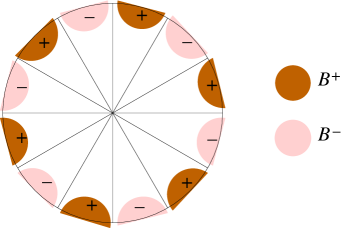
Figure 8: The regions $B^{\pm}$ for the case $k=4$.

As mentioned in section 3.2.1, the A-brane $\Scr{B}_{L,M,S}$ corresponds to the D1-brane at the wedge-shaped line $\gamma_{L,M,S}$ coming in from the direction $\arg(X)=\pi{M-L-1\over k+2}$, cornering at $X=0$, and going out to the direction $\arg(X)=\pi{M+L+1\over 2}$ if $S=0$ or $1$ ($S=2$ or $-1$ are their orientation reversals). The branes with $S=\pm 1$ preserve the supercharge $\overline{Q}_{+}+Q_{-}$ while those with $S=0,2$ preserves the opposite combination $\overline{Q}_{+}-Q_{-}$. The cycle $\gamma_{L,M,1}^{+}$ is obtained by slightly rotating $\gamma_{L,M,1}$, counter-clock-wise. This correspondence $\gamma_{L,M,S}\leftrightarrow|\Scr{B}_{L,M,S}\rangle$ is at the in-coming boundary. At the out-going boundary, the correspondence is slightly different: $\gamma_{L,M,1}$ (resp. $\gamma_{L,M,0}$) corresponds to $\langle\Scr{B}_{L,M-1,0}|$ (resp. $\langle\Scr{B}_{L,M-1,1}|$). This can be understood by comparing the RR-charges as well as the conserved worldsheet supersymmetries.

The parity ${\it g}^{m}P_{A}$ commutes with the worldsheet supercharge $\overline{Q}_{+}+Q_{-}$ which is preserved by branes $\gamma_{L,M,S}$ with odd $S$. It acts on the LG field as $X\rightarrow\,{\rm e}^{2\pi im\over k+2}\overline{X}$ and the O-plane $O_{{\it g}^{m}P_{A}}$ is the straight line at $X\in\,{\rm e}^{\pi im\over k+2}{\mathbb{R}}$. We assume the orientation that goes from $\arg(X)={\pi m\over k+2}$ to the opposite direction. Note that $m\rightarrow m+(k+2)$ is the orientation flip. The cycle $O_{{\it g}^{m}P_{A}}^{+}$ is obtained by deforming it so that both of the two asymptotics are in the region $B^{+}$. This involves bending when $k$ is odd while it is a small rotation when $k$ is even. To see this, let us first consider the basic A-parity $P_{A}$ whose O-plane $O_{P_{A}}$ is the real line that goes from $+\infty$ to $-\infty$. If $k$ is even, $O_{P_{A}}^{+}$ is the slight counter-clockwise rotation of ${\mathbb{R}}$. In fact there is an A-brane that does the same — $\gamma_{{k\over 2},{k+2\over 2},1}$. Thus, the O-plane $O_{P_{A}}$ and $\gamma_{{k\over 2},{k+2\over 2},1}$ has the same location and the same charge. If $k$ is odd, $O_{P_{A}}^{+}$ is obtained by small counter-clockwise rotation of the real-positive half and small clockwise rotation of the real-negative half. There is no A-brane at the same location, but the brane $\gamma_{{k-1\over 2},{k+1\over 2},1}$ has the same in-coming charge. (Another brane $\gamma_{{k-1\over 2},{k+1\over 2}+1,0}$ may appear to have the same charge, but it preserves a different combination $\overline{Q}_{+}-Q_{-}$ of the supercharge — $P_{A}$ preserves the combination $\overline{Q}_{+}+Q_{-}$ and thus must be compared to the branes with odd $S$.) Figure 9 depicts the example of $k=3$.

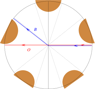
Figure 9: The O-plane $O=O_{P_{A}}$ and the brane $B=\gamma_{1,2,1}$ in the $k=3$ minimal model. They have the same in-coming RR-charge

Repeating this consideration in the general case, we find that the O-plane $O_{{\it g}^{m}P_{A}}$ has the same RR-charge as one of the A-branes. The result is

$$k [O_{{\it g}^{m}P_{A}}^{+}]=\left\{\begin{array}[]{ll}[\gamma_{{k\over 2},{k+2\over 2}+m,1}^{+}]&\mbox{$m$ even}\\ {[}\gamma_{{k\over 2},{k+2\over 2}+m-1,1}^{+}]&\mbox{$m$ odd},\end{array}\right.$$ even (4.7)

$$k [O_{{\it g}^{m}P_{A}}^{+}]=\left\{\begin{array}[]{ll}[\gamma_{{k-1\over 2},{k+1\over 2}+m,1}^{+}]&\mbox{$m$ even}\\ {[}\gamma_{{k+1\over 2},{k+1\over 2}+m,1}^{+}]&\mbox{$m$ odd}.\end{array}\right.$$ odd (4.10)

This can also be checked by showing ${}_{{{}_{\rm RR}}}\langle i|\Scr{C}_{{\it g}^{m}P_{A}}\rangle={}_{{{}_{\rm RR}}}\langle i|\Scr{B}_{L,M,S}\rangle_{{{}_{\rm RR}}}$ for any RR-ground state $|i\rangle_{{{}_{\rm RR}}}$ with $(L,M,S)$ as indicated in (4.7)-(4.10). Note that $m\rightarrow m+(k+2)$ indeed corresponds to orientation flip since RR-part of the corresponding boundary states flips its sign.

Having learned the RR-charge of the O-plane in the minimal model, we can now compute the charge in the Gepner model. For this purpose, the expressions (3.19) and (3.20) of the crosscap states are useful. These expressions simply says that the O-plane charge in the Gepner model is given by the same type of average formula for the A-brane charge.

If $H$ is odd, the average formula (3.19) is identical to the one for an A-brane. Note that we only have to consider the basic parity $P^{A}=P^{A}_{1;{\bf 0}}$ since there is no involutive dressing by quantum symmetry and dressing by global symmetry ${\bf m}$ is equivalent to no-dressing. By the relation (4.10) for each minimal model we find that the O-plane charge is the same as the charge of the D-brane associated with the product $\prod_{i=1}^{r}\Scr{B}_{{k_{i}-1\over 2},{k_{i}+1\over 2},1}$. Namely,

$$\Bigl{[}O_{P^{A}}\Bigr{]}=4\Bigl{[}B_{\bf{k-1\over 2},{k-1\over 2}}\Bigr{]},$$ (4.11)

where the factor of $4$ comes from the spacetime part.

If $H$ is even, the sum splits into two parts (3.20) and each part is the same as the untwisted part of the sum for an A-brane with ${\mathbb{Z}}_{2}$ stabilizer group. The charge for $|\Scr{C}_{{\bf P}^{A}_{\bf m}}\rangle$ is the same as the charge for the product brane $\prod_{i}\Scr{B}_{{k_{i}\over 2},{k_{i}+2\over 2}+m_{i}-\delta_{m_{i}},1}$ where

$$\delta_{m_{i}}=\left\{\begin{array}[]{ll}0&\mbox{$m_{i}$ even}\\ 1&\mbox{$m_{i}$ odd}.\end{array}\right.$$

The charge for $|\Scr{C}_{\gamma{\bf P}^{A}_{\bf m}}\rangle$ is the same as the charge for $-\prod_{i}\Scr{B}_{{k_{i}\over 2},{k_{i}+2\over 2}+m_{i}+\delta_{m_{i}},1}$, where the minus sign is from the factor $(-1)^{\sum_{i}{\nu\over k_{i}+2}}$ in (3.16). Thus, the charge is

$$\Bigl{[}O_{P^{A}_{\pm;{\bf m}}}\Bigr{]}=2\Bigl{[}B_{\bf{k\over 2},{k\over 2}+m-\delta_{m}}\Bigr{]}\mp 2\Bigl{[}B_{\bf{k\over 2},{k\over 2}+m+\delta_{m}}\Bigr{]},$$ (4.12)

where $[B_{\bf{k\over 2},M}]$ is the sum of the two short-orbit brane charges $[\widehat{B}_{\bf{k\over 2},M}^{(+)}]+[\widehat{B}_{\bf{k\over 2},M}^{(-)}]$ which has no twisted state component.

Let us discuss the spacetime supersymmetry preserved by D-branes and the O-plane. This is to compute the ratio of the overlap of the boundary/crosscap state with RR-ground state $|0\rangle_{{{}_{\rm RR}}}$ and the brane/plane tension. Here $|0\rangle_{{{}_{\rm RR}}}$ is the RR ground state of the internal system with the lowest R-charge. Let us first present the RR-overlap for the A-brane in the minimal model. This has been computed in many ways. In the LG description, it is realized as the integral over $\gamma_{L,M,1}^{+}$ of the 1-form $\overline{c_{0}}\,{\rm e}^{-i\overline{X}^{k+2}}*{\rm d}\overline{X}$ where $c_{0}$ is a certain normalization factor [54, 55, 18]. The result is

$${}_{{{}_{\rm RR}}}\langle 0|\Scr{B}_{L,M,1}\rangle_{{{}_{\rm RR}}} = i\sqrt{2\over(k+2)\sin({\pi\over k+2})}\,{\rm e}^{-\pi i{M\over k+2}}\sin\Bigl{(}{\pi(L+1)\over k+2}\Bigr{)}$$

$$= i\,{\rm e}^{-\pi i{M\over k+2}}{}_{{{}_{\rm NSNS}}}\langle 0|\Scr{B}_{L,M,1}\rangle_{{{}_{\rm NSNS}}}.$$

Using this, we find that the overlap in the Gepner model is

$${}_{{{}_{\rm RR}}}\langle 0|\Scr{B}_{{\bf L,M},1}\rangle_{{{}_{\rm RR}}}=i^{r}\,{\rm e}^{-\pi i\sum_{i}{M_{i}\over k_{i}+2}}{}_{{{}_{\rm NSNS}}}\langle 0|\Scr{B}_{{\bf L,M},1}\rangle_{{{}_{\rm NSNS}}}.$$

The phase determining the spacetime supersymmetry is the ratio

$$\exp\left(i\theta_{\bf L,M}\right)=-i\exp\left(-\pi i\sum_{i=1}^{r}{M_{i}\over k_{i}+2}\right).$$ (4.13)

We find that the phase is determined by the sum over the angles ${M_{i}\over k_{i}+2}$ of the “mean-direction” of the wedge in the LG realization. See Figure 10. The result is applicable also to short orbit branes.

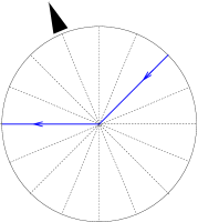
Figure 10: The mean direction of a brane.

Let us next compute the RR-overlap for the crosscap states. In the minimal model, this is essentially computed in [18], in both using PSS crosscap and also using LG model. Here one could also use the relation of the O-plane charge and D-brane charge given in (4.7) and (4.10) and the above expression for the brane overlaps. In any way, we find

$${}_{{{}_{\rm RR}}}\langle 0|\Scr{C}_{{\it g}^{m}P_{A}}\rangle = \left\{\begin{array}[]{ll}i\sqrt{2\over(k+2)\sin({\pi\over k+2})}\cos\Bigl{(}{\pi\over 2(k+2)}\Bigr{)}\,{\rm e}^{-\pi i{{k+1\over 2}+m\over k+2}}&\mbox{$k$ odd},\\[5.69046pt] i\sqrt{2\over(k+2)\sin({\pi\over k+2})}\,{\rm e}^{-\pi i{{k+2\over 2}+m-\delta_{m}\over k+2}}&\mbox{$k$ even}\end{array}\right.$$

$$= i\,{\rm e}^{-\pi i{m+{k+1\over 2}\over k+2}}\times{}_{{{}_{\rm NSNS}}}\langle 0|\Scr{C}_{{\it g}^{m}\widetilde{P}_{A}}\rangle.$$

It follows from this that in the Gepner model

$${}_{{{}_{\rm RR}}}\langle 0|\Scr{C}_{P_{\omega;{\bf m}}^{A}}\rangle=i^{r}\,{\rm e}^{-\pi i\sum_{i}{m_{i}+{k+1\over 2}\over k_{i}+2}}\times{}_{{{}_{\rm NSNS}}}\langle 0|\Scr{C}_{\widetilde{P}_{\omega;{\bf m}}^{A}}\rangle$$

Since the NSNS crosscap in string theory is obtained by multiplying $\omega^{1\over 2}$ to $|\Scr{C}_{\widetilde{P}_{\omega;{\bf m}}^{A}}\rangle$, we find that the ratio is

$$\exp\left(i\theta_{P^{A}_{\omega;{\bf m}}}\right)=-i\omega^{-{1\over 2}}\exp\left(-\pi i\sum_{i=1}^{r}{m_{i}+{k_{i}-1\over 2}\over k_{i}+2}\right).$$ (4.17)

The phase is essentially the sum over the slopes ${m_{i}+{k_{i}-1\over 2}\over k_{i}+2}$ of the direction perpendicular to the O-planes if $\omega=1$, but it differs from that sum by right angle if $\omega=-1$.

In Table 5, we describe the RR-charge, the tension, and the phase determining the conserved supersymmetry of the twelve A-type orientifolds of the two parameter model $(k_{i}+2)=(8,8,4,4,4)$.

parity	RR-charge	Tension	SUSY
$P^{B}_{+;00000}$	$0$	$0$	$i\omega^{-{1\over 2}}$
$P^{B}_{-;00000}$	$4[B_{{\bf k\over 2},{\bf k\over 2}}]$	$-i\omega^{1\over 2}2\sqrt{2\sqrt{2}+2}$
$P^{B}_{+;00001}$	$2[B_{{\bf k\over 2},{\bf k\over 2}}-B_{{\bf k\over 2},(33113)}]$	$\omega^{1\over 2}2\sqrt{\sqrt{2}+1}$	$i\omega^{-{1\over 2}}\,{\rm e}^{-{\pi i\over 4}}$
$P^{B}_{-;00001}$	$2[B_{{\bf k\over 2},{\bf k\over 2}}+B_{{\bf k\over 2},(33113)}]$	$-i\omega^{1\over 2}2\sqrt{\sqrt{2}+1}$
$P^{B}_{+;01000}$	$2[B_{{\bf k\over 2},{\bf k\over 2}}-B_{{\bf k\over 2},(35111)}]$	$2\omega^{1\over 2}$	$i\omega^{-{1\over 2}}\,{\rm e}^{-{\pi i\over 8}}$
$P^{B}_{-;01000}$	$2[B_{{\bf k\over 2},{\bf k\over 2}}+B_{{\bf k\over 2},(35111)}]$	$-2i\omega^{1\over 2}(\sqrt{2}+1)$
$P^{B}_{+;00011}$	$2[B_{{\bf k\over 2},{\bf k\over 2}}-B_{{\bf k\over 2},(33133)}]$	$\omega^{1\over 2}2\sqrt{2}\sqrt{\sqrt{2}+1}$	$\omega^{-{1\over 2}}$
$P^{B}_{-;00011}$	$2[B_{{\bf k\over 2},{\bf k\over 2}}+B_{{\bf k\over 2},(33133)}]$	$0$
$P^{B}_{+;01001}$	$2[B_{{\bf k\over 2},{\bf k\over 2}}-B_{{\bf k\over 2},(35113)}]$	$\omega^{1\over 2}2(\sqrt{2}+1)$	$i\omega^{-{1\over 2}}\,{\rm e}^{-{3\pi i\over 8}}$
$P^{B}_{-;01001}$	$2[B_{{\bf k\over 2},{\bf k\over 2}}+B_{{\bf k\over 2},(35113)}]$	$-2i\omega^{1\over 2}$
$P^{B}_{+;11000}$	$2[B_{{\bf k\over 2},{\bf k\over 2}}-B_{{\bf k\over 2},(55111)}]$	$\omega^{1\over 2}2\sqrt{\sqrt{2}+1}$	$i\omega^{-{1\over 2}}\,{\rm e}^{-{\pi i\over 4}}$
$P^{B}_{-;11000}$	$2[B_{{\bf k\over 2},{\bf k\over 2}}+B_{{\bf k\over 2},(55111)}]$	$-i\omega^{1\over 2}2\sqrt{\sqrt{2}+1}$

Table 5: Charge and Tension of O-planes in the two parameter model ($\omega=1$)

4.2 Parity Action on D-branes

The next task is to find out how the parities act on the D-branes.

Let us first consider the action in the minimal model, which is studied [18]. The action is encoded in the formulae

$$\langle\Scr{C}_{{\it g}^{m}P_{A}}|q_{t}^{H}|\Scr{B}_{L,M,S}\rangle_{{{}_{\rm RR}}}={}_{{{}_{\rm RR}}}\langle\Scr{B}_{L,2m-M-1,-S-1}|q_{t}^{H}|\Scr{C}_{(-1)^{F}{\it g}^{m}P_{A}}\rangle,$$ (4.18)

$$\langle\Scr{C}_{{\it g}^{m}\widetilde{P}_{A}}|q_{t}^{H}|\Scr{B}_{L,M}\rangle_{{{}_{\rm NSNS}}}={}_{{{}_{\rm NSNS}}}\langle\Scr{B}_{L,2m-M}|q_{t}^{H}|\Scr{C}_{(-1)^{F}{\it g}^{m}\widetilde{P}_{A}}\rangle.$$ (4.19)

They can be shown using the properties of the P-matrix $\,{\rm e}^{2\pi iQ_{g}(j)}P_{gj}^{*}=P_{gj}$. They can also be geometrically understood in the LG model as follows. Under the basic parity $P_{A}$ that acts on the LG field as $X\rightarrow\overline{X}$, the wedge $\gamma_{L,M,1}$ is mapped to its complex conjugate. The initial and final angles $({\pi(M-L-1)\over k+2},{\pi(M+L+1)\over k+2})$ of the wedge are mapped to $({\pi(-M+L+1)\over k+2},{\pi(-M-L-1)\over k+2})$ which are the initial and final angles of the wedge $\gamma_{L,-M,1}$ with the opposite orientation. Thus the brane $\gamma_{L,M,1}$ is mapped under $P_{A}$ to $-\gamma_{L,-M,1}=\gamma_{L,-M,-1}$. More general parity maps the brane as

$${\it g}^{m}P_{A}:\gamma_{L,M,1}\rightarrow\gamma_{L,2m-M,-1}.$$

Note that the parity exchanges in-coming and out-going boundaries. Thus, if $\gamma_{L,M,1}$ is at the in-coming boundary and corresponds to $|\Scr{B}_{L,M,1}\rangle$, then $\gamma_{L,2m-M,-1}$ is at the out-going boundary and corresponds to $\langle\Scr{B}_{L,2m-M-1,-2}|$. Thus we find that the parity acts as

$${\it g}^{m}P_{A}:|\Scr{B}_{L,M,1}\rangle\rightarrow\langle\Scr{B}_{L,2m-M-1,-2}|.$$

This is nothing but the $S=1$ case of (4.18). The one with other values of $S$ and the other relation (4.19) can also be understood in a similar way.

Let us now discuss the orientifold action on D-branes in the full string theory. The relations (4.18) and (4.19) readily imply

$$\langle\Scr{C}_{P^{A}_{\omega;{\bf m}}}|q_{t}^{H}|\Scr{B}_{{\bf L,M},S}\rangle_{{{}_{\rm RR}}}={}_{{{}_{\rm RR}}}\langle\Scr{B}_{{\bf L,2m-M-1},-S-1}|q_{t}^{H}|\Scr{C}_{(-1)^{F}P^{A}_{\omega;{\bf m}}}\rangle,$$ (4.20)

$$\langle\Scr{C}_{\widetilde{P}^{A}_{\omega;{\bf m}}}|q_{t}^{H}|\Scr{B}_{\bf L,M}\rangle_{{{}_{\rm NSNS}}}={}_{{{}_{\rm NSNS}}}\langle\Scr{B}_{\bf L,2m-M}|q_{t}^{H}|\Scr{C}_{(-1)^{F}\widetilde{P}^{A}_{\omega;{\bf m}}}\rangle.$$ (4.21)

Applying these to the total crosscap states, we find

$${}_{{{}_{\rm RR}}}\langle C_{\omega;{\bf m}}|q_{t}^{H}|B_{\bf L,M}\rangle_{{{}_{\rm RR}}}=\omega\times{}_{{{}_{\rm RR}}}\langle B_{\bf L,2m-M}|q_{t}^{H}|C_{\omega;{\bf m}}\rangle_{{{}_{\rm RR}}},$$ (4.22)

$${}_{{{}_{\rm NSNS}}}\langle C_{\omega;{\bf m}}|q_{t}^{H}|B_{\bf L,M}\rangle_{{{}_{\rm NSNS}}}=-{}_{{{}_{\rm NSNS}}}\langle B_{\bf L,2m-M}|q_{t}^{H}|C_{\omega;{\bf m}}\rangle_{{{}_{\rm NSNS}}}.$$ (4.23)

Recall that the overlaps appears in the one-loop diagram as the combination

$$i{}_{{{}_{\rm NSNS}}}\langle B|q_{t}^{H}|C\rangle_{{{}_{\rm NSNS}}}-i{}_{{{}_{\rm NSNS}}}\langle C|q_{t}^{H}|B\rangle_{{{}_{\rm NSNS}}}-{}_{{{}_{\rm RR}}}\langle B|q_{t}^{H}|C\rangle_{{{}_{\rm RR}}}-{}_{{{}_{\rm RR}}}\langle C|q_{t}^{H}|B\rangle_{{{}_{\rm RR}}}.$$

Thus the equation (4.23) shows that the brane $B_{\bf L,M}$ is mapped to $B_{\bf L,2m-M}$ if the brane orientations are ignored. The first equation includes the information on the orientations. It shows that the branes are mapped under the orientifold action as

$$P^{A}_{\omega;{\bf m}}:\,B_{\bf L,M}\longmapsto\omega B_{\bf L,2m-M},$$ (4.24)

where $-B$ stands for the orientation reversal of $B$. We see that dressing by quantum symmetry affects the action on orientation.

Let us see how the short-orbit branes are transformed. We recall that if $L_{i}={k_{i}\over 2}$ for each $i$ with odd $w_{i}$ (possible only when $H$ is even), the brane $B_{\bf L,M}$ must be regarded as the sum of two short-orbit branes $\widehat{B}_{\bf L,M}^{(+)}$ and $\widehat{B}_{\bf L,M}^{(-)}$. The boundary states are given in (3.42) and (3.43). The overlap $\langle\widehat{B}^{(\pm)}|C\rangle$ is simply one-half of $\langle B|C\rangle$ for both $\pm$, since the crosscap state $|C\rangle$ does not have twisted state components. Thus we see that the $({\bf L,M})$-label is transformed in the same way as the long-orbit branes. To see how the $\pm$ label is transformed, we need to compare with the $\langle\widehat{B}^{(\varepsilon)}|\widehat{B}^{(\varepsilon^{\prime})}\rangle$ overlaps. By the loop channel expansion of the latter overlaps, one can read the spectrum of open string states between two short-orbit branes: the states labeled by $\otimes_{i=1}^{r}(l_{i},m_{i},s_{i})$ are subject to the projection

$$\frac{1}{2}\left(\,1+\varepsilon\varepsilon^{\prime}\prod_{w_{i}~{}{\rm odd}}(-1)^{\frac{1}{2}(l_{i}+m_{i}-s)}\,\right),$$ (4.25)

where $s=0$ for NS states and $1$ for R ones. Let us compare this with the loop-channel expansion of the overlaps $\langle\widehat{\Scr{B}}|q_{t}^{H}|\Scr{C}\rangle$. It turns out that the open string states are subject to the projection

$$\frac{1}{2}\left(\,1+\omega^{\frac{H}{2}}(-1)^{\frac{\sigma}{2}}\prod_{w_{i}~{}{\rm odd}}(-1)^{\frac{1}{2}(l_{i}+m_{i}-s)}\,\right),$$ (4.26)

where $\sigma$ is the number of $i$’s such that $w_{i}$ is odd. The parity action on short-orbit branes is therefore summarized as

$$P^{A}_{\omega;{\bf m}}~{}:~{}\widehat{B}_{\bf L,M}^{(\varepsilon)}\longmapsto\omega\widehat{B}_{\bf L,2m-M}^{(\varepsilon^{\prime})},~{}~{}~{}\varepsilon^{\prime}=\omega^{\frac{H}{2}}(-1)^{\frac{\sigma}{2}}\varepsilon.$$ (4.27)

For the computations that leads to (4.25) and (4.26), see Appendix B.

4.2.1 Invariant Branes

Let us see which of the branes are invariant under the parity symmetries. By (4.24), the long-orbit brane $B_{\bf L,M}$ is invariant under $P^{A}_{\omega;\bf m}$ when $\omega B_{\bf L,2m-M}=B_{\bf L,M}$. This requires that, for each $i$, $\Scr{B}_{L_{i},2m_{i}-M_{i},0}$ is equal to $\Scr{B}_{L_{i},M_{i},0}$ up to orientation (and up to the uniform shift in $M_{i}$’s). One possibility is $L_{i}$ arbitrary and $2m_{i}-M_{i}=M_{i}$ (mod $2k_{i}+4$) which is the case with the positive orientation, and another is $L_{i}=k_{i}/2$ and $2m_{i}-M_{i}=M_{i}+k_{i}+2$ (mod $2k_{i}+4$) which is the case with the reversed the orientation. For $\omega=1$, we need the total orientation to be positive, and thus the case “$L_{i}=k_{i}/2$ and $2m_{i}-M_{i}=M_{i}+k_{i}+2$” must occur for even number of $i$’s:

$$P^{A}_{+;{\bf m}}\mbox{-fixed}:\left\{\begin{array}[]{ll}L_{i}={k_{i}\over 2},\,\,\,M_{i}=m_{i}+{k_{i}+2\over 2}\,\,(\mbox{mod $k_{i}+2$}),&\mbox{for even \# of $i$'s}\\ L_{i}\,\,\mbox{arbitrary,}\,\,\,M_{i}=m_{i}\,\,\,(\mbox{mod $k_{i}+2$}),&\mbox{for other $i$}\end{array}\right.$$ (4.28)

For $\omega=-1$ (which is possible only when some $k_{i}$ are even), we need the total orientation to be negative, and thus the case “$L_{i}=k_{i}/2$ and $2m_{i}-M_{i}=M_{i}+k_{i}+2$” must occur for odd number of $i$’s:

$$P^{A}_{-;{\bf m}}\mbox{-fixed}:\left\{\begin{array}[]{ll}L_{i}={k_{i}\over 2},\,\,\,M_{i}=m_{i}+{k_{i}+2\over 2}\,\,(\mbox{mod $k_{i}+2$}),&\mbox{for odd \# of $i$'s}\\ L_{i}\,\,\mbox{arbitrary,}\,\,\,M_{i}=m_{i}\,\,\,(\mbox{mod $k_{i}+2$}),&\mbox{for other $i$}\end{array}\right.$$ (4.29)

Let us next consider the short orbit branes $\widehat{B}_{\bf L,M}^{(\varepsilon)}$. For this case, the “Brane Identification” involves the change in $\varepsilon$-label: $M_{i}\rightarrow M_{i}+k_{i}+2$ for $i$ with odd $w_{i}$ does the flip of $\varepsilon$ in addition to the flip of orientation. Also, the parity acts on the $\varepsilon$ label as

$$\varepsilon\rightarrow\omega^{\frac{H}{2}}(-1)^{\frac{\sigma}{2}}\varepsilon.$$

Thus, the invariant branes are those with

$$\left\{\begin{array}[]{ll}L_{i}={k_{i}\over 2},\,\,\,M_{i}=m_{i}+{k_{i}+2\over 2}\,\,(\mbox{mod $k_{i}+2$}),&i\in I\\ L_{i}\,\,\mbox{arbitrary,}\,\,\,M_{i}=m_{i}\,\,\,(\mbox{mod $k_{i}+2$}),&i\not\in I\end{array}\right.$$

where $I$ is a subset of $\{1,...,r=5\}$ obeying some condition that depends on the parity and case as described in the table.

	$P^{A}_{+;{\bf m}}$, ${\sigma\over 2}$ even	$P^{A}_{+;{\bf m}}$, ${\sigma\over 2}$ odd	$P^{A}_{-;{\bf m}}$, ${\sigma+H\over 2}$ even	$P^{A}_{-;{\bf m}}$, ${\sigma+H\over 2}$ odd
$\#I$	even	even	odd	odd
$\#(I\cap\Sigma)$	even	odd	even	odd

Here $\Sigma$ is the set of $i$’s with odd $w_{i}$ ($\sigma=\#\Sigma$).

4.3 Structure of Chan-Paton Factor

Let us now determine the structure of Chan-Paton factor on the D-branes. If not with orientifolds, $N$ D-branes on top of each other, i.e., $N$ copies of a D-brane, support $U(N)$ gauge group. In the orientifold model, this is modified. If the D-brane $B_{a}$ is not invariant under the parity, $P:B_{a}\rightarrow B_{a}^{\prime}\neq B_{a}$, the gauge group is still $U(N)$ since $B_{a}$-$B_{a}$ string is simply related to $B_{a}^{\prime}$-$B_{a}^{\prime}$ string under the orientifold projection. However, for an invariant D-brane, a non-trivial projection is imposed on the open string ending on it, and the gauge group is usually either $O(N)$ or $USp(N)=Sp(N/2)$. In the latter case $N$ must be even, which is one of the consistency requirement.

Thus, we would like to find the orientifold projections on invariant D-branes. Let $\psi^{\mu}_{-{1\over 2}}|IJ\rangle$ ($1\leq I,J\leq N$) be the open string states corresponding to the massless gauge bosons. The parity action is

$$\psi^{\mu}_{-{1\over 2}}|IJ\rangle\mapsto-\sum_{I^{\prime}J^{\prime}}\gamma_{II^{\prime}}\psi^{\mu}_{-{1\over 2}}|J^{\prime}I^{\prime}\rangle\gamma^{-1}_{J^{\prime}J}$$

where $\gamma^{T}=\pm\gamma$ is required for the parity to be involutive. The gauge group is $O(N)$ if $\gamma^{T}=\gamma$ (solved by $\gamma={\bf 1}_{N}$) and $Sp({N\over 2})$ if $\gamma=-\gamma^{T}$ (solved by $\gamma={{\bf 0}\,-{\bf 1}\choose{\bf 1}\,\,\,\,{\bf 0}}$). One consequence is that

$${\rm Tr}\Bigl{|}_{\rm gauge\,\,boson}Pq^{H}=-2{\rm tr}(\gamma^{T}\gamma^{-1})q^{1\over 2}=-2N\sigma q^{1\over 2},$$

where

$$\sigma=\left\{\begin{array}[]{ll}1&\mbox{if $O(N)$}\\ -1&\mbox{if $Sp({N\over 2})$}.\end{array}\right.$$ (4.30)

Thus, to find out the type of the Chan-Paton factor, we want to look at the sign in front of the gauge boson part $q^{0}$ in the twisted partition function ${\rm Tr}Pq^{H}=i\langle B|q_{t}^{H}|C\rangle$.

It is straightforward to compute the $\langle B|C\rangle$ overlaps of the minimal model and their loop-channel expansions. In particular, the ground state contribution is

$${}_{{{}_{\rm NSNS}}}\langle\Scr{B}_{L,M,S}|q_{t}^{H}|\Scr{C}_{2m,0}(\mp)\rangle=\left\{\begin{array}[]{l}\,{\rm e}^{\mp{\pi i\over 4}}\delta_{M,m}\delta_{S,0}\\ \,{\rm e}^{\pm{\pi i\over 4}}\delta_{M,m}\delta_{S,1}\\ \,{\rm e}^{\pm{\pi i\over 4}}\delta_{L,{k\over 2}}\delta_{M,m+{k+2\over 2}}\delta_{S,0}\\ \,{\rm e}^{\mp{\pi i\over 4}}\delta_{L,{k\over 2}}\delta_{M,m+{k+2\over 2}}\delta_{S,1}\end{array}\right\}\times\widehat{\chi}_{0,0,0}(q_{l})+\cdots$$ (4.31)

where the delta functions are mod $k+2$ for $M$-indices and mod 2 for $S$-indices. For the universal part, we find

$$\langle\Scr{B}_{+}|q_{t}^{H}|\Scr{C}_{+}\rangle_{{{}_{\rm NSNS}}}=\langle\Scr{B}_{-}|q_{t}^{H}|\Scr{C}_{-}\rangle_{{{}_{\rm NSNS}}}=\,{\rm e}^{-{\pi i\over 4}}q^{-{1\over 2}}\prod_{n=1}^{\infty}(1-i(-1)^{n}q_{l}^{n-{1\over 2}})^{2},$$

$$\langle\Scr{B}_{+}|q_{t}^{H}|\Scr{C}_{-}\rangle_{{{}_{\rm NSNS}}}=\langle\Scr{B}_{-}|q_{t}^{H}|\Scr{C}_{+}\rangle_{{{}_{\rm NSNS}}}=\,{\rm e}^{{\pi i\over 4}}q^{-{1\over 2}}\prod_{n=1}^{\infty}(1+i(-1)^{n}q_{l}^{n-{1\over 2}})^{2},$$

up to the factors from bosonic transverse oscillators, longitudinal modes, and ghost/superghost sectors. Combining the above equations, we find

$$\langle B_{\bf L,M}|q_{t}^{H}|C_{\omega;{\bf m}}\rangle_{{{}_{\rm NSNS}}}$$ (4.32)

$$= \!\!\omega^{-{1\over 2}}\,{\rm e}^{{\pi i\over 4}(-1+r_{1}-r_{2})}q^{-{1\over 2}}\prod_{n=1}^{\infty}(1-i(-1)^{n}q_{l}^{n-{1\over 2}})^{2}-\omega^{1\over 2}\,{\rm e}^{{\pi i\over 4}(1-r_{1}+r_{2})}q^{-{1\over 2}}\prod_{n=1}^{\infty}(1+i(-1)^{n}q_{l}^{n-{1\over 2}})^{2}$$

$$+\cdots$$

up to the universal factor, where we have decomposed $r$ as $r_{1}+r_{2}$;

$$\begin{array}[]{l}r_{1}=\#\{i|M_{i}=m_{i}\}\\ r_{2}=\#\{i|L_{i}={k_{i}\over 2},M_{i}=m_{i}+{k_{i}+2\over 2}\}\end{array}$$

Note that

$$\omega^{1\over 2}\,{\rm e}^{{\pi i\over 4}(1-r_{1}+r_{2})}=\,{\rm e}^{{\pi i\over 4}(1-r)}\omega^{1\over 2}\,{\rm e}^{{\pi i\over 2}r_{2}}=-\omega^{1\over 2}\,{\rm e}^{{\pi i\over 2}r_{2}}$$

where $r=5$ is used. It is a sign factor since $r_{2}$ is even for $\omega=1$, and $r_{2}$ is odd if $\omega=-1$. This is the sign $\sigma$ that determines the structure of Chan-Paton factor. $N$ D-branes support $O(N)$ gauge group if it is $+1$ while they support $Sp(N/2)$ gauge group if it is $-1$:

$$-\omega^{1\over 2}\,{\rm e}^{{\pi i\over 2}r_{2}}=\left\{\begin{array}[]{lcl}1&\Longrightarrow&O(N),\\[5.69046pt] -1&\Longrightarrow&Sp({N\over 2}).\end{array}\right.$$

For example, consider the case where $\omega^{1\over 2}=-1$. Then, the branes with $M_{i}=m_{i}$ for all $i$ support $O(N)$ gauge group, those with two $i$’s with $L_{i}={k_{i}\over 2},M_{i}=m_{i}+{k_{i}+2\over 2}$ support $Sp(N/2)$ gauge group, and those with four $i$’s with $L_{i}={k_{i}\over 2},M_{i}=m_{i}+{k_{i}+2\over 2}$ support $O(N)$ gauge group.

To see the LG image of this rule, let us look at the two kinds of invariant branes in the minimal model, one with $M=m$ another with $L={k\over 2}$, $M=m+{k+2\over 2}$.

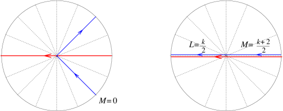
Figure 11: Two branes invariant under the parity with $m=0$.

The $M=m$ branes intersect transversely with the O-plane and the $L={k\over 2}$, $M={k+2\over 2}$ branes are parallel to the O-plane. We have seen above that replacing transverse branes by parallel brane in two factors flips the type of the CP factor from $O(N)$ to $Sp({N\over 2})$ and vice versa. Note that two factors means real four-dimensions. This is very much reminiscent of what happens in the standard superstring in flat space. For example, consider a Type II orientifold with an O7-plane. If D7-branes parallel to O7-plane support $O(N)$, D7-branes intersecting orthogonally to O7-plane in real four-dimensions support $Sp({N\over 2})$. (This is what happens if we obtain this system by T-duality from Type I and decompactification [56], but we could also consider the opposite case — parallel branes support $Sp({N\over 2})$ and orthogonal branes support $O(N)$.)

The result (4.3) applies also to short-orbit branes, since the overlap with the crosscap state does not receive contribution from the twisted sector.

4.4 A Class of Consistent and Supersymmetric D-brane Configurations

We have obtained the expression of the charge and the supersymmetry of the O-plane, and we also described the orientifold action on rational D-branes and the structure of CP-factor of the invariant D-branes. Thus we have obtained the condition of consistency as well as the spacetime supersymmetry on the D-brane configurations. Now, we are interested in finding solutions. It is not an easy task to classify all solutions because the rank of the charge lattice is very large (typically 100) and also there are many D-branes preserving the unbroken supersymmetry. In this subsection, we present special solutions. In the case with odd $H$, we find one solution in each case. In the case with even $H$, we present an algorithm to find a solution. It works in most of the cases but sometimes it fails.

To simplify the notation, we consider the O-plane of the reversed orientation. Namely, we use $-|C_{\omega;{\bf m}}\rangle_{{{}_{\rm RR}}}$ in place of the RR-crosscap state. For this choice the RR-charge and the phase for the spacetime supersymmetry (e.g. the ones in the table of page 5) have extra minus sign.

4.4.1 Odd $H$

If $H$ is odd, we have seen that the RR-charge of the crosscap state is equal to the RR-charge of one of the D-branes, which is $B_{\bf{k-1\over 2},{k-1\over 2}}$. One can also see that this brane preserves the same spacetime supersymmetry unbroken by the orientifold — the phases (4.13) and (4.17) are both $-i^{r}\exp(-\pi i\sum_{i}{k_{i}-1\over 2(k_{i}+2)})$. Furthermore, this brane is invariant under the orientifold action. This can be shown as follows. As we found above, the brane is mapped to $B_{\bf{k-1\over 2},-{k-1\over 2}}$. Here, we note that $H=(k_{i}+2)w_{i}$ where $w_{i}$ is an integer — in fact $w_{i}$ is an odd integer in the present case where $H$ is odd. This means that $H\equiv k_{i}+2$ mod $2(k_{i}+2)$, or

$$(H-3)\equiv k_{i}-1\quad\mbox{mod $2(k_{i}+2)$}.$$

Using this we find that the orientifold action is

$$P^{A}:B_{\bf{k-1\over 2},{k-1\over 2}}\longrightarrow B_{\bf{k-1\over 2},-{k-1\over 2}}=B_{{\bf{k-1\over 2},-{k-1\over 2}}+(H-3){\bf 1}}=B_{\bf{k-1\over 2},{k-1\over 2}}.$$

Namely the brane $B_{\bf{k-1\over 2},{k-1\over 2}}$ is mapped to itself under the orientifold action.

Thus, we find that a consistent and spacetime supersymmetric configuration is given by four $B_{\bf{k-1\over 2},{k-1\over 2}}$’s. This may be regarded as the configuration of four D-branes “on top of” the O-plane, although we do not have a geometrical picture.

One consequence of this result is that, when continued on the Kähler moduli space from the Gepner point to a large volume limit, the branes $B_{\bf{k-1\over 2},{k-1\over 2}}$ becomes the D-brane wrapped on the D6-brane wrapped on the fixed point set of the involution $\tau:X_{i}\rightarrow\overline{X}_{i}$. For example, the D-brane wrapped on the real quintic in the quintic hypersurface in ${{\mathbb{C}}{\mathbb{P}}}^{4}$ is the continuation of $B_{{\bf 1,1}}$.

4.4.2 Even $H$

If $H$ is even, the RR-charge of the O-plane is expressed as in (4.12) as the sum or the difference of the untwisted part of the RR-charge of two kinds of branes, $B_{\bf{k\over 2},{k\over 2}+m-\delta_{m}}$ and $B_{\bf{k\over 2},{k\over 2}+m+\delta_{m}}$. However, generically the two preserve different combinations of supersymmetry as one can see from their phases, and in particular, neither one of them preserve the supersymmetry unbroken by the orientifold. In order to preserve spacetime supersymmetry, one has to find the set of D-branes all with the same phase whose RR-charge in total equals that of the O-plane. We study the example $(k_{i}+2)=(8,8,4,4,4)$ in detail.

$\bullet$ $P^{A}_{\pm;00000}$
This is a special case in which the two D-branes are the same. For the $P^{A}_{+;00000}$-orientifold, the O-plane has no RR charge and hence it gives a consistent supersymmetric configuration without adding any D-branes. For the $P^{A}_{-;00000}$-orientifold, the O-plane charge is equal to $-4[B_{\bf{k\over 2},{k\over 2}}]=-4[\widehat{B}_{\bf{k\over 2},{k\over 2}}^{(+)}+\widehat{B}_{\bf{k\over 2},{k\over 2}}^{(-)}]$. Thus, four $\widehat{B}^{(+)}_{\bf{k\over 2},{k\over 2}}$ and four $\widehat{B}^{(-)}_{\bf{k\over 2},{k\over 2}}$ provide a tadpole canceling brane configuration. Note that the twisted part of the RR-charge carried by the $(+)$-brane and the $(-)$-brane cancel against each other. One can also see that they preserve the same supersymmetry unbroken by the orientifold with $\omega^{1\over 2}=-i$. The $+$ branes and $-$ branes are exchanged with each other under the orientifold. Hence the gauge group supported by the branes is $U(4)$.

$\bullet$ $P^{A}_{\pm;00001}$
The O-plane charge is given by

$$[O_{P^{A}_{\pm;00001}}]~{}=~{}-2[\widehat{B}_{{\bf k\over 2},(33111)}]\pm 2[\widehat{B}_{{\bf k\over 2},(33113)}].$$

The two D-branes indeed preserve different combinations of supersymmetry since the $M$-labels of the 5-th factor are different. Let us now focus on this factor. As one can see from Fig. 12,

Figure 12: The recombination of the branes for $\gamma_{1,1}+\gamma_{1,3}$ (middle) and $\gamma_{1,1}-\gamma_{1,3}$ (right).

the sum and the difference of the two charges can be recombined as follows (to simplify the notation, we denote $\gamma_{L,M+1,1}$ by $\gamma_{L,M}$):

$$[\gamma^{+}_{1,1}]-[\gamma^{+}_{1,3}]~{}=~{}[\gamma^{+}_{2,0}]+[\gamma^{+}_{0,0}],\quad[\gamma^{+}_{1,1}]+[\gamma^{+}_{1,3}]~{}=~{}[\gamma^{+}_{2,2}]+[\gamma^{+}_{0,2}].$$

In either case, the two resulting wedges have a common “mean-direction”. This shows that the two new D-branes that result from the recombination preserve the same supersymmetry. The new D-branes are $B_{\bf L_{1},M_{1}}$ and $B_{\bf L_{2},M_{1}}$ for $\omega=1$ and $\widehat{B}_{\bf L_{1},M_{2}}$ and $\widehat{B}_{\bf L_{2},M_{2}}$ for $\omega=-1$, where

$${\bf L_{1}}=(33110),\,\,{\bf L_{2}}=(33112),\,\,{\bf M_{1}}=(33110),\,\,{\bf M_{2}}=(33112).$$

They split into the sum of the $(+)$ and the $(-)$ short orbit branes. Thus, we find supersymmetric and tadpole-canceling configurations are given by:

$$\mbox{\text@underline{two each of $\widehat{B}^{(+)}_{\bf L_{1},M_{1}}$, $\widehat{B}^{(-)}_{\bf L_{1},M_{1}}$, $\widehat{B}^{(+)}_{\bf L_{2},M_{1}}$, $\widehat{B}^{(-)}_{\bf L_{2},M_{1}}$ for $P^{A}_{+;00001}$-orientifold ($\omega^{1\over 2}=-1$)}},$$

two each of $$\widehat{B}^{(+)}_{\bf L_{1},M_{2}} \widehat{B}^{(-)}_{\bf L_{1},M_{2}} \widehat{B}^{(+)}_{\bf L_{2},M_{2}} \widehat{B}^{(-)}_{\bf L_{2},M_{2}} P^{A}_{-;00001} \omega^{1\over 2}=-i$$, , , for -orientifold ().

Again, we need the same number of $+$ branes and $-$ branes to cancel the twisted part of the RR-tadpole. In both cases, the $+$ branes and the $-$ branes are exchanged by the orientifold action (${\bf L_{i}}$ fixed for $P^{A}_{+;00001}$ and exchanged for $P^{A}_{-;00001}$). Therefore the gauge group is $U(2)\times U(2)$.

$\bullet$ $P^{A}_{\pm;01000}$
O-plane charge is proportional to the difference or the sum of $B_{{\bf k\over 2},(33111)}$ and $B_{{\bf k\over 2},(35111)}$. For this case, we focus of the second factor. The recombination relevant for this is depicted in Fig. 13.

Figure 13: The recombination of branes for $\gamma_{3,3}+\gamma_{3,5}$ (middle) and $\gamma_{3,3}-\gamma_{3,5}$ (right).

In each case, the “mean-directions” of the two wedges are aligned after the recombination. We also note that, in each of these cases, the two branes are mapped into each other by rotation of four steps. To be precise, the orientation is revered but that is compensated by the orientation reversal for the $L={k_{1}\over 2}$ brane of the first factor. Thus, they are in the same (long) orbit of the ${\mathbb{Z}}_{8}$ orbifold group. We therefore found a supersymmetric and tadpole-canceling configuration: four $B_{\bf L_{3},M_{3}}$ for the $P^{A}_{+;01000}$-orientifold ($\omega^{1\over 2}=-1$) and four $B_{\bf L_{4},M_{4}}$ for the $P^{A}_{-;01000}$-orientifold ($\omega^{1\over 2}=-i$), where

$${\bf L_{3}}=(30111),\quad{\bf M_{3}}=(30111),\quad{\bf L_{4}}=(32111),\quad{\bf M_{4}}=(34111).$$

These branes are invariant under the respective orientifolds. The gauge group is $O(4)$ for both $P^{A}_{+;01000}$ ($\omega^{1\over 2}=-1$) and $P^{A}_{-;01000}$ ($\omega^{1\over 2}=-i$).

$\bullet$ $P^{A}_{\pm;00011}$
O-plane charge is proportional to the difference or the sum of $B_{{\bf k\over 2},(33111)}$ and $B_{{\bf k\over 2},(33133)}$. For this case, we need to focus on the two factors, 4-th and 5-th. The recombination to align the “mean-directions” is not obvious, but we can use the following trick. It is to use the identity

$$A_{1}A_{2}-B_{1}B_{2}={1\over 2}(A_{1}+B_{1})(A_{2}-B_{2})+{1\over 2}(A_{1}-B_{1})(A_{2}+B_{2}).$$

For the $P^{A}_{+;00011}$-orientifold, we find

$$(\gamma_{1,1})^{2}-(\gamma_{1,3})^{2} = {1\over 2}(\gamma_{1,1}+\gamma_{1,3})(\gamma_{1,1}-\gamma_{1,3})+{1\over 2}(\gamma_{1,1}-\gamma_{1,3})(\gamma_{1,1}+\gamma_{1,3})$$

$$= {1\over 2}(\gamma_{0,2}+\gamma_{2,2})(\gamma_{0,0}+\gamma_{2,0})+{1\over 2}(\gamma_{0,0}+\gamma_{2,0})(\gamma_{0,2}+\gamma_{2,2})$$

where we have used the recombination used in the case of $P^{A}_{\pm;00001}$. This indeed aligns the sum of “mean-directions”, and thus a supersymmetry is preserved — it is the one preserved by the $\omega^{1\over 2}=-1$ orientifold. The resulting brane configuration is the collection of sixteen branes $\widehat{B}^{(\pm)}_{\bf L_{i},M_{j}}$, $i=5,6,7,8$, $j=5,6$ where

$${\bf L_{5}}=(33100),\,\,{\bf L_{6}}=(33102),\,\,{\bf L_{7}}=(33120),\,\,{\bf L_{8}}=(33122),$$

$${\bf M_{5}}=(33120),\,\,{\bf M_{6}}=(33102).$$

The orientifold exchanges the $+$ and $-$ labels (and acts on the ${\bf L_{i}}$ labels in a certain way). Thus the gauge group is $U(1)^{8}$.

For the $P^{A}_{-;00011}$-orientifold, the same procedure on the 4-th and 5-th factors gives

$$(\gamma_{1,1})^{2}+(\gamma_{1,3})^{2}={1\over 2}(\gamma_{0,0}+\gamma_{2,0})^{2}+{1\over 2}(\gamma_{0,2}+\gamma_{2,2})^{2}$$

and the sum of the “mean-directions” are not aligned. (The two terms have opposite phases.) Thus, this recipe of recombination does not work to find a supersymmetric configuration. In fact, in this case, the O-plane tension is vanishing (see the table in page 5), and there is no supersymmetric brane configuration that cancels the RR-tadpole.

$\bullet$ $P^{A}_{\pm;01001}$
This case is similar to the above. For the $P^{A}_{+;01001}$-orientifold, the recombination successfully aligns the “mean-direction” and we find that a supersymmetric and tadpole canceling configuration is given by two each of $B_{\bf L_{9},M_{7}}$, $B_{\bf L_{10},M_{7}}$, $B_{\bf L_{11},M_{8}}$ and $B_{\bf L_{12},M_{8}}$, where

$${\bf L_{9}}=(32110),\,\,{\bf L_{10}}=(32112),\,\,{\bf L_{11}}=(30110),\,\,{\bf L_{12}}=(30112),$$

$${\bf M_{7}}=(34110),\,\,{\bf M_{8}}=(30112).$$

The preserved supersymmetry is that of $\omega^{1\over 2}=-1$. ${\bf M}={\bf M_{7}}$ branes are invariant under the orientifold action and are of $Sp$-type, whereas the two ${\bf M}={\bf M_{8}}$ branes are mapped to each other. Thus the gauge group is $Sp(1)\times Sp(1)\times U(2)$.

For the $P^{A}_{-;01001}$-orientifold, recombination does not work.

$\bullet$ $P^{A}_{\pm;11000}$
For the $P^{A}_{+;11000}$-orientifold, a supersymmetric and tadpole canceling configuration is given by two each of $B_{\bf L_{13},M_{9}}$, $B_{\bf L_{14},M_{9}}$, $B_{\bf L_{15},M_{10}}$ and $B_{\bf L_{16},M_{10}}$, where

$${\bf L_{13}}=(20111),\,\,{\bf L_{14}}=(26111),\,\,{\bf L_{15}}=(02111),\,\,{\bf L_{16}}=(04111),$$

$${\bf M_{9}}=(40111),\,\,{\bf M_{10}}=(04111).$$

The preserved supersymmetry is that of $\omega^{1\over 2}=-1$. Orientifold action preserves the ${\bf M}$-label but exchanges the ${\bf L}$-labels as ${\bf L_{13}}\leftrightarrow{\bf L_{14}}$ and ${\bf L_{15}}\leftrightarrow{\bf L_{16}}$. Thus the gauge group is $U(2)\times U(2)$.

For the $P^{A}_{-;11000}$-orientifold, recombination does not work.

4.5 Particle Spectra in Some Supersymmetric Models

Let us find out the spectrum of massless particles for the configurations obtained in the previous subsection. The problem here is to count the numbers of scalar fields in various open string sectors and study the action of parity on them. They are read off from the annulus and Möbius strip amplitudes. Here are some essential facts:

• The open string states $\otimes_{i}(l_{i},n_{i},s_{i})$ between two D-branes $B_{\bf L,M}$ and $B_{\bf L^{\prime},M^{\prime}}$ satisfy $n_{i}=M^{\prime}_{i}-M_{i}+2\nu$ mod $(2k_{i}+4)$, and $l_{i}$’s are also constrained from the $SU(2)$ fusion rule.

• Massless scalars correspond to chiral or antichiral primary states $\otimes_{i}(l_{i},l_{i},0)$ or $\otimes_{i}(l_{i},-l_{i},0)$ with $\sum_{i}\frac{l_{i}}{k_{i}+2}=1$. They are the lowest components of four-dimensional ${\cal N}=1$ chiral or antichiral multiplets, and are related to each other by the worldsheet orientation reversal. Namely, chiral primary states on $B-B^{\prime}$ string and antichiral primary states on $B^{\prime}-B$ string are related to each other.

• For the open string states on the parity invariant D-branes we have to study the action of parity. If the brane $B_{\bf L,M}$ is invariant under the parity $P^{A}_{\omega,{\bf m}}$, the open strings $\otimes_{i}(l_{i},n_{i},s_{i})$ on the Möbius strip satisfy $n_{i}=2M_{i}-2m_{i}+2\nu$ mod $(2k_{i}+4)$, and the constraint on $l_{i}$ from the $SU(2)$ fusion rule. For chiral or antichiral states satisfying the above two conditions, the parity eigenvalue is then given by

  $$P=-i\omega^{\nu-\frac{1}{2}}(-i)^{\{\#{\rm of}\,(s_{i}=2)\}},$$ (4.33)

  where we have to put $\omega^{\frac{1}{2}}=-1$ or $-i$ for $\omega=\pm 1$ as before.

We present here the relevant amplitudes that lead to the above conclusions. (We describe them for general $r$ and $d$ but we are interested in the case $r=5$ and $d=1$.) The NS part of the annulus amplitude between the A-branes $B_{\bf L,M}$ and $B_{\bf L^{\prime},M^{\prime}}$ is given by

$$\frac{1}{2}\sum_{\nu=1}^{H}\sum_{l_{i}}\prod_{i=1}^{r}N_{L_{i}L^{\prime}_{i}}^{~{}l_{i}}\times\left\{\chi^{\rm(st)NS+}\prod_{i=1}^{r}\chi^{\rm NS+}_{l_{i},M^{\prime}_{i}-M_{i}+2\nu}-\chi^{\rm(st)NS-}\prod_{i=1}^{r}\chi^{\rm NS-}_{l_{i},M^{\prime}_{i}-M_{i}+2\nu}\right\}$$ (4.34)

where $\chi^{\rm NS\pm}_{l,n}=\chi_{l,n,0}\pm\chi_{l,n,2}$ are linear combinations of minimal model characters and $\chi^{\rm(st)NS\pm}$ represent the non-compact spacetime ${\mathbb{R}}^{2d+2}$ plus ghost contribution

$$\chi^{\rm(st)NS\pm}=q^{-\frac{d}{8}}(1\pm 2d\cdot q^{\frac{1}{2}}+\cdots).$$ (4.35)

For pairs of short-orbit branes, the sum over the open string states is subject to the projection

$$\frac{1}{4}(1+\varepsilon\bar{\varepsilon}\prod_{w_{i}~{}{\rm odd}}(-1)^{\frac{1}{2}(l_{i}+M^{\prime}_{i}-M_{i})})$$ (4.36)

The NS part of Möbius strip amplitude between the A-brane $B_{\bf L,M}$ and its image under the parity $P^{A}_{\omega;\bf m}$ is given by

$${\rm Re}\left\{ie^{\frac{\pi i(r-d)}{4}}\sum_{\nu=1}^{H}\sum_{l_{i}}\omega^{-\frac{1}{2}-\nu}\hat{\chi}^{\rm(st)NS+}\prod_{i=1}^{r}N_{L_{i}L_{i}}^{~{}l_{i}}\hat{\chi}^{\rm NS+}_{l,2M_{i}-2m_{i}+2\nu}\right\},$$ (4.37)

where $\hat{\chi}^{\rm(st)NS\pm}$ represent the spacetime and ghost contributions

$$\hat{\chi}^{\rm(st)NS\pm}=q^{-\frac{d}{8}}(1\pm 2id\cdot q^{\frac{1}{2}}+\cdots)$$ (4.38)

and $\hat{\chi}^{\rm NS\pm}_{l,n}$ are defined by

$$\hat{\chi}^{\rm NS\pm}_{l,n}=(-1)^{\frac{1}{2}(l+n)}(\hat{\chi}_{l,n,0}\pm i\hat{\chi}_{l,n,2}),~{}~{}~{}\hat{\chi}_{l,n,s}(\tau)=\,{\rm e}^{-\pi i(\frac{l(l+2)-n^{2}}{4k+8}+\frac{s^{2}}{8}-\frac{c}{24})}\chi_{l,n,s}(\tau+1/2).$$ (4.39)

For short-orbit branes the amplitude gets an extra factor of $\frac{1}{2}$. It is easy to read off the parity eigenvalue (4.33) for (anti)chiral primary states from this formula.

4.5.1 Odd $H$

We have seen that the configuration of four $B_{\bf\frac{k-1}{2},\frac{k-1}{2}}$’s in the $P^{A}_{+,{\bf 0}}$-orientifold is supersymmetric and free of tadpoles, and the gauge symmetry is $O(4)$ in all cases. However, the spectrum of massless matters depends on the model. Let us illustrate here our analysis in some examples.

$k_{i}=(33333)$
On the annulus and on the Möbius strip we find one chiral primary state $\otimes_{i=1}^{5}(2,6,2)$ which is equivalent to $\otimes_{i=1}^{5}(1,1,0)$. Since this has $P=1$, there is one chiral multiplet belonging to the symmetric tensor representation 10 of $O(4)$.

$k_{i}=(11777)$
There are two chiral multiplets, which appear on the Möbius strip as chiral primary states $\otimes_{i=1,2}(0,4,2)\otimes_{i=3,4,5}(6,10,2)$ and $\otimes_{i=1,2}(0,0,0)\otimes_{i=3,4,5}(4,12,2)$ respectively. The former has $P=1$ while the latter has $P=-1$, so they belong to one symmetric and one antisymmetric tensor representations of $O(4)$.

The analysis of other models goes in much the same way. The result is summarized in the table below.

($k_{i}$)	(3,3,3,3,3)	(1,1,7,7,7)	(1,3,3,3,13)	(1,1,3,13,13)	(1,1,5,5,19)	(1,1,3,7,43)
$\#{\bf 10}$	1	1	2	2	2	8
$\#{\bf 6}$	0	1	1	1	3	3

4.5.2 Even $H$ – two parameter model $k_{i}=(66222)$ in detail

$\bullet$ $P^{A}_{-;00000}$
Four short-orbit branes $\widehat{B}^{(+)}_{\bf\frac{k}{2},\frac{k}{2}}$ and their parity images support $U(4)$ gauge symmetry, and there is a single adjoint matter.

$\bullet$ $P^{A}_{\pm;00001}$
The structure of massless spectrum are the same for the two examples

$$P^{A}_{+;00001}: 2\widehat{B}^{(+)}_{\bf L_{1},M_{1}}+2\widehat{B}^{(-)}_{\bf L_{1},M_{1}}+2\widehat{B}^{(+)}_{\bf L_{2},M_{1}}+2\widehat{B}^{(-)}_{\bf L_{2},M_{1}},$$

$$P^{A}_{-;00001}: 2\widehat{B}^{(+)}_{\bf L_{1},M_{2}}+2\widehat{B}^{(-)}_{\bf L_{1},M_{2}}+2\widehat{B}^{(+)}_{\bf L_{2},M_{2}}+2\widehat{B}^{(-)}_{\bf L_{2},M_{2}},$$

with ${\bf L_{1}}=(33110),\,\,{\bf L_{2}}=(33112),\,\,{\bf M_{1}}=(33110),\,\,{\bf M_{2}}=(33112).$ In both cases, the gauge group is $U(2)\times U(2)$ and there are matters in the representation $({\bf 2,\bar{2}})\oplus({\bf\bar{2},2})$.

$\bullet$ $P^{A}_{\pm;01000}$
Here we found the configurations with four long-orbit branes which are invariant under the parity. The $P^{A}_{+;01000}$-orientifold with four $B_{(30111),(30111)}$ gives

$$O(4)$$ pure Super-Yang-Mills.

The $P^{A}_{-;01000}$-orientifold with four $B_{(32111),(34111)}$ gives

$$O(4)$$ with one symmetric and one antisymmetric matters.

$\bullet$ $P^{A}_{+;00011}$
Here we find a very interesting situation. The tadpole canceling configuration we have found is eight short-orbit branes $B_{\rm I},\cdots,B_{\rm VIII}$ and their parity images, where

$$\begin{array}[]{rclrclrclrcl}B_{\rm I}&=&\widehat{B}^{(+)}_{{\bf L_{5},M_{5}}},&B_{\rm II}&=&\widehat{B}^{(+)}_{{\bf L_{6},M_{5}}},&B_{\rm III}&=&\widehat{B}^{(+)}_{{\bf L_{7},M_{5}}},&B_{\rm IV}&=&\widehat{B}^{(+)}_{{\bf L_{8},M_{5}}},\\ B_{\rm V}&=&\widehat{B}^{(+)}_{{\bf L_{5},M_{6}}},&B_{\rm VI}&=&\widehat{B}^{(+)}_{{\bf L_{6},M_{6}}},&B_{\rm VII}&=&\widehat{B}^{(+)}_{{\bf L_{7},M_{6}}},&B_{\rm VIII}&=&\widehat{B}^{(+)}_{{\bf L_{8},M_{6}}},\end{array}$$

with ${\bf L_{5}}=(33100)$, ${\bf L_{6}}=(33102)$, ${\bf L_{7}}=(33120)$, ${\bf L_{8}}=(33122)$, ${\bf M_{5}}=(33120)$, and ${\bf M_{6}}=(33102)$. The gauge group is $U(1)^{8}$, and we have quite a few matter fields which are charged under two of $U(1)$’s. The spectrum are the most neatly expressed in terms of the quiver diagram, where each arrow represents a chiral multiplet charged $+1$ and $-1$ under the $U(1)$’s on its head and tail.

Figure 14: quiver diagram representing a D-brane configuration with $P^{A}_{+;00011}$

Note that the gauge theory is chiral. There is a mixed $U(1)_{a}U(1)_{b}^{2}$ anomaly for each pair $(a,b)$ of neighboring groups of the quiver (i.e. VII-I,IV-VII,VI-IV,VI-I for the first square, and similarly for the second square). Anomaly cancellation mechanism will be discussed in Section 5.2.

$\bullet$ $P^{A}_{+;01001}$
For this parity we found a tadpole canceling configuration

$$2B_{\bf L_{9},M_{7}}+2B_{\bf L_{10},M_{7}}+2B_{\bf L_{11},M_{8}}+2B_{\bf L_{12},M_{8}}$$

with ${\bf L_{9}}=(32110)$, ${\bf L_{10}}=(32112)$, ${\bf L_{11}}=(30110)$, ${\bf L_{12}}=(30112)$, ${\bf M_{7}}=(34110)$, and ${\bf M_{8}}=(30112)$. The gauge group is $Sp(1)\times Sp(1)\times U(2)$ and there are matters in the representations

$$\bf{\rm 2\times}(2,2,1)\oplus(2,1,2)\oplus(1,2,\bar{2}).$$

This system is also chiral. There are mixed $U(1)Sp(1)_{a}^{2}$ anomalies. Anomaly cancellation mechanism will be discussed in Section 5.2.

$\bullet$ $P^{A}_{+;11000}$
We found a D-brane configuration

$$2B_{\bf L_{13},M_{9}}+2B_{\bf L_{14},M_{9}}+2B_{\bf L_{15},M_{10}}+2B_{\bf L_{16},M_{10}}$$

with ${\bf L_{13}}=(20111)$, ${\bf L_{14}}=(26111)$, ${\bf L_{15}}=(02111)$, ${\bf L_{16}}=(04111)$, ${\bf M_{9}}=(40111)$, and ${\bf M_{10}}=(04111)$. The gauge group is $U(2)\times U(2)$, and the matter belongs to $\bf(2,\bar{2})\oplus(\bar{2},2)$.

4.6 More general tadpole canceling configurations

In the previous subsection, we have seen that it is generically rather easy to find a supersymmetric tadpole canceling brane configuration for Type IIA orientifolds of Gepner models. When all levels are odd, these configurations corresponds to placing $4$ D-branes on top of the O-plane, and leads to $O(4)$ gauge group with some matter content which depends on the particular model. On the other hand, we have seen that when some levels are even, we can have somewhat more interesting configurations which support unitary gauge groups and chiral matter.

It would be interesting to know whether these are all solutions and if not, how to describe the set of all possibilities. Let us recall the general nature of the problem. First of all, we emphasize once again that we have only been considering certain rational boundary states, which are just a subset of all possible branes that could be used to cancel the tadpoles. It would be interesting to see if one can obtain more interesting possibilities by using for example the boundary states constructed in [57] (which are still rational, but more general than the ones we have considered here). Secondly, we wish to point out that the problem of finding tadpole canceling configurations does not actually depend on whether we are considering Type IIA or Type IIB (the two are just exchanged by mirror symmetry). In other words, it is sufficient to discuss the conditions (4.1) in the internal CFT.

With these comments in mind, we are looking for sets of rational D-branes which

(i) have the same RR-charge as the O-plane,

(ii) are invariant under the parity,

(iii) allow a consistent assignment of Chan-Paton factor,

and, if we are interested in spacetime supersymmetric configurations,

(iv) preserve a common ${\mathcal{N}}=1$ supersymmetry.

These conditions are solved in steps.
Step 1: Choose the parity $P$. Compute the RR-charge $[O_{P}]$ and the preserved spacetime supersymmetry $M_{O}$ of the corresponding O-plane.
Step 2: Make a list of rational branes $B_{i}$ preserving the same spacetime supersymmetry as the O-plane, and compute their RR-charges $[B_{i}]$. We note that we have to distinguish branes even if they have the same RR charge.
Step 3: Determine for each brane its image $B_{P(i)}$ under the parity. If a brane is fixed under the parity, determine whether the gauge group is of $O$ or $Sp$-type. We will use an indicator $\sigma_{i}$ to concisely denote this gauge group. If the gauge group supported on $n_{i}$ branes $[B_{i}]$ is $O(n_{i})$, we will set $\sigma_{i}=+1$, if it is of type $Sp(n_{i}/2)$ we set $\sigma_{i}=-1$. If the brane is not invariant under $P$ (so the gauge group is $U(n_{i})$), we will set $\sigma_{i}=0$.
Step 4: Solve the equation

$$\sum_{i}n_{i}[B_{i}]=[O_{P}]$$ (4.40)

for positive integers $n_{i}$ under the condition that $n_{i}=n_{P(i)}$ and that $n_{i}$ is even if $\sigma_{i}=-1$.

Steps 1-3 are of course just those that we have been taking above. The hard part is solving (4.40). Indeed, while this is a linear equation, there are a large number of equations to solve (on the order of $100$ RR charges) and a large number of variables (on the order of several thousands branes preserving the same supersymmetry as any given O-plane). The number of solutions to this Diophantine problem is finite when restricted to positive integers $n_{i}$, because there is always one equation in which all $n_{i}$ appear with a positive coefficient. The simplest way to obtain this equation is to take the overlap with the RR ground state $|0\rangle_{\rm RR}$. By eq. (4.2), this is proportional to the overlap with the NSNS ground state, so what we are saying is simply that the tensions of the branes are all positive and must cancel the tension of the O-plane.

Knowing that the number of solutions is finite, one would like to count or even enumerate the solutions. A priori, it is not even clear that there is a single one (besides the somewhat trivial ones we have already found). To estimate the difficulty of the problem, we notice that the tension of the A-type orientifold in the quintic is about (minus) 20 times the typical tension of A-branes. So if we try to scan all the configurations in which the tension of D-branes cancel the negative tension of orientifold, there are roughly $\left({2000\atop 20}\right)\sim 10^{50}$ of them, which is too large a number to look through even with the help of a computer. One has to resort to a more direct method.

The problem becomes dramatically simpler when the number of equations and the number of possible branes is smaller. For B-type on the quintic, for example, there are $2$ linearly independent equations and $32$ variables. This problem (and its analogs for the two parameter model) can be solved completely, as we do in section 6. If we consider the orbifold of the quintic by a certain ${\mathbb{Z}}_{5}$ phase symmetry (see [25]), it turns out that there are $6$ equations in $96$ variables. This problem is still tractable, and we present some solutions in appendix D.

A purely technical difficulty is to find the right basis in which to write the equations (4.1). The simplest basis might seem to be the basis of RR ground states which are products of the minimal model ground states in the form

$$|l_{i}\rangle=\prod_{i=1}^{5}|l_{i},l_{i}+1,1\rangle\times|l_{i},-l_{i}-1,-1\rangle\qquad(1\leq l_{i}+1\leq k_{i}+1,~{}\sum_{i}{\textstyle\frac{l_{i}+1}{k_{i}+2}}\in{\mathbb{Z}})$$ (4.41)

However, the problem is that when written in this basis, the Diophantine equations (4.40) are not manifestly integral — the coefficients are certain combinations of trigonometric and exponential functions. To remedy this situation, one can use the fact that (at the level of charges) some branes can be written as integral linear combinations of other branes. A convenient choice of reference branes — for any Gepner model — are the branes with ${\bf L}={\bf 0}$ and varying ${\bf M}$. This “basis” has often been used in previous works on the RS boundary states in Gepner models. We note three important facts.
(i) The ${\bf L}={\bf 0}$ branes in general only generate a sublattice of the full BPS charge lattice. As we have mentioned before, the generic Gepner model has chiral ring elements from twisted sectors, corresponding to non-toric blowups in the geometry. The corresponding RR fields do not couple to the RS branes, which preserve a diagonal chiral algebra in each minimal model.
(ii) The ${\bf L}={\bf 0}$ branes are not in general primitive generators of the charge lattice. It is an outstanding problem to find boundary states which are integral generators of the charge lattice.
(iii) The charges of the ${\bf L}={\bf 0}$ branes are not linearly independent. It can sometimes be a little cumbersome to eliminate these relations in (iii) in order to find the linearly independent conditions. We discuss how this can be done in appendix C.

O(4) Configuration is Not Always Possible

To conclude this section, we answer (in the negative) the following question: At large volume, the tadpole of the O6-plane is always exactly canceled by the four D-branes all wrapping on it. Can we always find a corresponding solution at the Gepner point? We have found such a configuration for each of odd $H$ Gepner models. However, in the model with even $H$ one cannot always find such a configuration. In the two parameter model, it turns out that the only such solutions are those for $P^{A}_{\pm,01000}$ found already.

To see this, let us first look at the tensions of the O-planes. For the $P^{A}_{\omega;{\bf m}}$-orientifold, it is related to the tension of the D-brane $B_{(33111),{\bf M}}$ by

$$T_{O^{A}_{+;{\bf m}}} = -4\sin{\textstyle\frac{\pi n}{8}}T_{(33111),{\bf M}},$$

$$T_{O^{A}_{-;{\bf m}}} = -4\left|\cos{\textstyle\frac{\pi n}{8}}\right|T_{(33111),{\bf M}}$$

where $n:=\sum_{i}w_{i}m_{i}$ if we assume $m_{i}=0$ or $1$. One can show that there is no $O(4)$ configurations when $n\!=\!0$ or $4$, in the following way. In these cases the O-plane tension, if nonvanishing, is equal to $-4T_{(33111),{\bf M}}$, but the brane $B_{(33111),{\bf M}}$ is sum of two short orbit branes. Moreover, any elementary brane has tension less that $T_{(33111),{\bf M}}$. Thus, the O-plane tension cannot be canceled with just four identical elementary branes. For $n=1,2$ or $3$ the tensions are rewritten as

$$T_{O^{A}_{+;{\bf m}}} = -4T_{(3,n-1,1,1,1),{\bf M}}~{}=~{}-4T_{(n-1,3,1,1,1),{\bf M}},$$

$$T_{O^{A}_{-;{\bf m}}} = -4T_{(3,3-n,1,1,1),{\bf M}}~{}=~{}-4T_{(3-n,3,1,1,1),{\bf M}}$$

and similarly for $n=5,6,7$. There are no other branes with the same tension. Thus the only configurations with four identical D-branes that can cancel the O-plane tensions are

$$\begin{array}[]{c}P^{A}_{+;00001}\Rightarrow 4B_{(31111),{\bf M}}~{},\\ P^{A}_{+;01000}\Rightarrow 4B_{(30111),{\bf M}}~{},\\ P^{A}_{+;01001}\Rightarrow 4B_{(32111),{\bf M}}~{},\\ P^{A}_{+;11000}\Rightarrow 4B_{(31111),{\bf M}}~{},\end{array}~{}~{}\begin{array}[]{c}P^{A}_{-;00001}\Rightarrow 4B_{(31111),{\bf M}}~{},\\ P^{A}_{-;01000}\Rightarrow 4B_{(32111),{\bf M}}~{},\\ P^{A}_{-;01001}\Rightarrow 4B_{(30111),{\bf M}}~{},\\ P^{A}_{-;11000}\Rightarrow 4B_{(31111),{\bf M}}{}\end{array}$$

and those obtained by exchanging $L_{1}$ and $L_{2}$.

Let us then see whether any of the above relations are lifted to the full equality between the RR-charges. The possibilities in the first and the fourth rows can be easily excluded by looking at their transformation property under the permutations of the first two minimal models. Also, those in the first and the third rows are excluded because the branes cannot be parity invariant under any choice of ${\bf M}$ label. This is easily seen by noting that, for the branes $B_{\bf L,M}$ in the two parameter model to be invariant under $P^{A}_{\omega,{\bf m}}$, $M_{i}-m_{i}$ have to be all even or all add. Thus we are left with the ones in the second row, for which the permutation of minimal models, parity invariance and $O(4)$ gauge symmetry reduce the possibilities to

$$P^{A}_{+;01000}\Rightarrow 4B_{(30111),(30111)}\,,~{}~{}P^{A}_{+;01000}\Rightarrow 4B_{(30111),(12111)}\,,~{}~{}P^{A}_{-;01000}\Rightarrow 4B_{(32111),(34111)}\,.$$

Two of them are the configurations that was already found before. The remaining (second) case does not satisfy the full tadpole condition, as can be guessed from the comparison with the first one and confirmed by a more detailed analysis of the tadpole condition.

5 Chirality, Anomaly Cancellation, and Fayet-Iliopoulos Terms

In this section, we take a break and make some general remarks on chirality, anomaly cancellation mechanism, and Fayet-Iliopoulos terms.

5.1 Chirality and Witten Indices

Chirality of the theory can be measured by the open string Witten indices of the internal CFT,

$$I(B,B^{\prime})={\rm Tr}\!\!\mathop{}_{{\mathcal{H}}_{\Scr{B},\Scr{B}^{\prime}}}(-1)^{F_{\rm int}},$$

$$I(B,O_{P})={\rm Tr}\!\!\mathop{}_{{\mathcal{H}}_{\Scr{B},P(\Scr{B})}}(-1)^{F_{\rm int}}P.$$

To see this, note that the GSO operator can be written as the product $(-1)^{F}=(-1)^{F_{\rm int}}(-1)^{F_{\rm st}}$. The spacetime part $(-1)^{F_{\rm st}}$ acts on the RR sector states, that is, on the spacetime fermions, as the gamma-five matrix, $\Gamma^{5}=\Gamma^{0}\Gamma^{1}\Gamma^{2}\Gamma^{3}$. Thus, by the GSO projection, the Witten index of the internal part ${\rm Tr}(-1)^{F_{\rm int}}$ is proportional to ${\rm Tr}_{\rm massless}\Gamma^{5}$, which measures the chirality of the theory.

Let $B$ and $B^{\prime}$ be branes that are not the orientifold images of each other, $P(B)\neq B^{\prime}$. The parity maps the $B$-$B^{\prime}$ string to the $P(B^{\prime})$-$P(B)$ string, and hence the orientifold projection simply relates the two string sectors. The chirality of the bifundamental representation is given by the index

$$\#(\overline{\bf n}_{B},{\bf n}_{B^{\prime}})-\#({\bf n}_{B},\overline{\bf n}_{B^{\prime}})=I(B,B^{\prime}).$$ (5.1)

By definition, it must be antisymmetric with respect to the exchange of $B$ and $B^{\prime}$. This is guaranteed by the antisymmetry of the index in the internal CFT, $I(B^{\prime},B)=-I(B,B^{\prime})$.

The string stretched from a brane $B$ to its parity image $P(B)$ is invariant under the parity action. Its Chan-Paton factor is $\overline{\bf n}_{B}\otimes{\bf n}_{P(B)}=\overline{\bf n}_{B}\otimes\overline{\bf n}_{B}$, the second rank tensor product of $\overline{\bf n}_{B}$. The orientifold projection selects the symmetric tensor times the $P=1$ states as well as the antisymmetric tensor times the $P=-1$ states. Note that the ordinary $B$-$P(B)$ index is the sum of the index in the $P=1$ subspace and the one in the $P=-1$ subspace, while the twisted index is the difference. Thus, the chirality of the symmetric and antisymmetric representation is

$$\#{\rm S}^{2}\overline{\bf n}_{B}-\#{\rm S}^{2}{\bf n}_{B}={1\over 2}\Bigl{(}I(B,P(B))+I(B,O_{P})\Bigr{)}$$ (5.2)

$$\#{\rm A}^{2}\overline{\bf n}_{B}-\#{\rm A}^{2}{\bf n}_{B}={1\over 2}\Bigl{(}I(B,P(B))-I(B,O_{P})\Bigr{)}$$ (5.3)

They must vanish if the brane is parity invariant, $P(B)=B$, and the representation $\overline{\bf n}_{B}$ is real or pseudo-real. This is again guaranteed by the antisymmetry of the indices $I(P(B),B)=-I(B,P(B))$, $I(O_{P},P(B))=-I(B,O_{P})$.

5.1.1 Examples in IIA Gepner Models

Let us study the Witten index of branes in Type IIA orientifolds of Gepner model. Long-orbit A-branes are simply the sum over images under the orbifold group ${\mathbb{Z}}_{H}$. Accordingly, the index is also given by the sum of the product of the minimal model indices

$$I(B_{\bf L,M},B_{\bf L^{\prime},M^{\prime}})=\sum_{\nu=0}^{H-1}\prod_{i=1}^{5}I(B_{L_{i},M_{i}},B_{L_{i}^{\prime},M_{i}^{\prime}+2\nu}).$$ (5.4)

Furthermore, the index for each minimal model is given by the intersection number of the wedge cycle, $I(B_{L_{i},M_{i}},B_{L_{i}^{\prime},M_{i}^{\prime}})=\#(\gamma_{L_{i},M_{i}}^{-}\cap\gamma_{L_{i}^{\prime},M_{i}^{\prime}}^{+})$. In many supersymmetric brane configurations, there are two or more branes with the same ${\bf M}$-label. So let us examine such a pair, $B_{\bf L,M}$ and $B_{\bf L^{\prime},M}$. In the LG picture, the two product branes $\prod_{i}\gamma_{L_{i},M_{i}}$ and $\prod_{i}\gamma_{L^{\prime}_{i},M_{i}}$ have the common mean-direction at each minimal model factor. After rotation by the orbifold group they no longer have the same mean-direction, but there is an interesting relation between different steps of rotation: $\gamma_{L^{\prime}_{i},M_{i}}^{+}$ rotated by a step $\nu$ and $\gamma_{L^{\prime}_{i},M_{i}}^{+}$ rotated by the opposite step $-(\nu+1)$ have the opposite intersection number with any $\gamma_{L_{i},M_{i}}$:

$$\#(\gamma_{L_{i},M_{i}}^{-}\cap\gamma_{L_{i}^{\prime},M_{i}^{\prime}+2\nu}^{+})=-\#(\gamma_{L_{i},M_{i}}^{-}\cap\gamma_{L_{i}^{\prime},M_{i}^{\prime}-2\nu-2}^{+}).$$

It follows that the $\nu$-th term in (5.4) is opposite to the $(H-1-\nu)$-th term, and the sum vanishes. Thus, we find the

Vanishing Theorem:
The index between two long-orbit branes of the same ${\bf M}$-label vanishes.

This helps us in finding chiral pairs of branes in a given model: If two D-branes have the same ${\bf M}$-labels, we find that they are non-chiral before analyzing the spectrum. We will see a similar vanishing theorem in Type IIB orientifolds.

Supersymmetry does not require that the branes to have the same ${\bf M}$-label but only that $\sum_{i}{M_{i}\over k_{i}+2}$ to be the same (modulo $H$). Indeed, in the examples we have studied, there are many configurations with various ${\bf M}$-labels. For example, consider the $P^{A}_{+;01001}$-orientifold with the branes $B_{\bf L_{9},M_{7}}$, $B_{\bf L_{10},M_{7}}$, $B_{\bf L_{11},M_{8}}$ and $B_{\bf L_{12},M_{8}}$ (two each). We find

$$I(B_{\bf L_{9},M_{7}},B_{\bf L_{11},M_{8}})=1,\quad I(B_{\bf L_{9},M_{7}},B_{\bf L_{12},M_{8}})=-1.$$

Indeed, we have seen that this system is chiral by an explicit spectrum analysis.

5.2 Anomaly Cancellation Mechanism

Let us consider a tadpole canceling brane configuration $\{n_{a}B_{a}\}$ in a Type II orientifold with respect to a worldsheet parity symmetry $P$. The gauge group $G_{a}$ supported by the $n_{a}$ branes $B_{a}$ is $U(n_{a})$ if $B_{a}$ is not invariant under the parity while it is $G_{a}=O(n_{a})$ or $Sp(n_{a}/2)$ if the brane is invariant. The tadpole cancellation condition is

$$\sum_{a}n_{a}[B_{a}]=[O_{P}].$$

The standard triangle anomalies in the low energy field theory are proportional to

$$A_{U(n_{a})U(n_{b})^{2}}=I(B_{a},B_{b})+I(B_{a},B_{P(b)})$$ (5.5)

$$A_{U(n_{a}){\rm Gravi}^{2}}=\sum_{b}I(B_{a},B_{b})n_{b}=I(B_{a},O_{P}).$$ (5.6)

where tadpole cancellation condition is used in the second equation. For the $U(n_{a})G_{b}^{2}$ anomaly with $G_{b}=O(n_{b})$ or $Sp(n_{b}/2)$, it is simply $I(B_{a},B_{b})$ (no extra term $I(B_{a},B_{P(b)})$ as in (5.5)). Note that only the $U(1)_{a}$ subgroup of $U(n_{a})$ is anomalous.

This field theory anomaly is canceled by the Green-Schwarz mechanism [58, 59, 60, 61]. The relevant Green-Schwarz terms are obtained from the disc diagrams with bulk insertion of a RR axion $\vartheta^{\bf i}$ and one or two boundary insertion of the gauge bosons, or from the ${{\mathbb{R}}{\mathbb{P}}}^{2}$ diagrams with insertion of a $\vartheta^{\bf i}$ and two gravitons. They are proportional to the overlaps

$$\Pi_{{\bf i}}^{a}=\langle\Scr{B}_{a}|\,{\rm e}^{-\pi iJ_{0}}|{\bf i}\rangle_{{{}_{\rm RR}}},\quad\widetilde{\Pi}^{b}_{\bf i}={}_{{{}_{\rm RR}}}\langle{\bf i}|\Scr{B}_{b}\rangle,\quad\widetilde{\Pi}^{P}_{\bf i}={}_{{{}_{\rm RR}}}\langle{\bf i}|\Scr{C}_{P}\rangle,$$

and are given by

$$\Pi_{\bf i}^{a}A^{U(1)_{a}}_{\mu}\partial^{\mu}\vartheta^{\bf i}$$ (5.7)

and

$$(\widetilde{\Pi}^{b}_{\bf i}+\widetilde{\Pi}^{P(b)}_{\bf i})\vartheta^{\bf i}{\rm Tr}_{\bf n_{b}}F^{b}\wedge F^{b},\qquad\widetilde{\Pi}^{P}_{\bf i}\vartheta^{\bf i}{\rm Tr}R\wedge R.$$

Note that the axion $\vartheta^{\bf i}$ corresponds to the RR ground state $|{\bf i}\rangle_{{{}_{\rm RR}}}$ that survives the orientifold projection. If there are $2(h+1)$ RR ground states obeying the same R-charge selection rule as the boundary states, the number of such $|{\bf i}\rangle_{{{}_{\rm RR}}}$ is $(h+1)$. Also, we have chosen a basis such that the overlaps $\Pi^{a}_{\bf i}$, $\widetilde{\Pi}^{b}_{\bf i}$ are real. The coupling (5.7) induces an anomalous $U(1)_{a}$ gauge transformation of the axion

$$\vartheta^{\bf i}\longrightarrow\vartheta^{\bf i}+g^{\bf ij}\Pi_{\bf j}^{a}\lambda_{a},$$

where $g^{\bf ij}$ is the inverse matrix of $g_{\bf ij}={}_{{{}_{\rm RR}}}\langle{\bf j}|{\bf i}\rangle_{{{}_{\rm RR}}}$ which determines the axion kinetic term, $g_{\bf ij}\partial^{\mu}\vartheta^{\bf i}\partial_{\mu}\vartheta^{\bf j}$. Then, the triangle anomalies are canceled as a consequence of the bilinear identity

$$\sum_{\bf i,j}\Pi^{a}_{\bf i}g^{\bf ij}(\widetilde{\Pi}^{b}_{\bf j}+\widetilde{\Pi}^{P(b)}_{\bf j})=I(B_{a},B_{b})+I(B_{a},B_{P(b)}),\qquad\sum_{\bf i,j}\Pi^{a}_{\bf i}g^{\bf ij}\widetilde{\Pi}^{P}_{\bf j}=I(B_{a},O_{P}).$$

The bilinear identity holds for the sum over all RR ground states [18]. However, in the present case, the sum can be restricted to the orientifold-invariant states $|{\bf i}\rangle_{{{}_{\rm RR}}}$, because $(\widetilde{\Pi}^{b}_{i}+\widetilde{\Pi}^{P(b)}_{i})$ and $\widetilde{\Pi}^{P}_{i}$ are non-vanishing only for such $|{\bf i}\rangle_{{{}_{\rm RR}}}$. Same is true on the overlap $\widetilde{\Pi}_{i}^{b}$ for a parity invariant brane, $P(b)=b$.

For Type IIA orientifolds of a Calabi-Yau manifold $M$, the RR-ground states $|i\rangle_{{{}_{\rm RR}}}$ contributing to the overlap $\Pi_{i}^{a}$ with A-branes corresponds to middle dimensional forms, and the axions are the KK reduction of the RR 3-form on $H^{3}(M)$. At the Gepner point, the rational A-branes have overlap only with the untwisted states since the boundary states are sum over images. Thus the Green-Schwarz mechanism works with the untwisted RR-fields, as long as rational A-branes are concerned. Similar situations are encountered in the context of toroidal orbifold in [62, 63].

For Type IIB orientifolds of a Calabi-Yau manifold $M$, the RR-ground states $|i\rangle_{{{}_{\rm RR}}}$ contributing to the overlap $\Pi_{i}^{a}$ with B-branes corresponds to diagonal forms, $H^{p,p}(M)$, and the axions are the KK reduction of the RR 0, 2, 4-forms. At the Gepner point, the rational B-branes generically have overlap with the twisted sector states since the boundary state is sum over twists. Thus the Green-Schwarz mechanism works with the twisted RR-fields, just as in Type I orbifolds studied in [61] (see also [64]).

5.3 Fayet-Iliopoulos Terms

The coupling (5.7) is extended to the full kinetic term $(\partial_{\mu}\vartheta^{\bf i}+g^{\bf ij}\Pi_{\bf j}^{a}A_{\mu}^{U(1)_{a}})^{2}$, and its supersymmetric completion is

$$\int{\rm d}^{4}\theta\,\,K\Bigl{(}Y^{\bf i}+\overline{Y^{\bf i}}+g^{\bf ij}\Pi_{\bf i}^{a}V_{a}\Bigr{)}.$$ (5.8)

Here $Y^{\bf i}$ is a chiral superfield whose lowest component is a complex scalar whose imaginary part is the axion $y^{\bf i}=c^{\bf i}-i\vartheta^{\bf i}$. This means that the real part $c^{\bf i}$ enters into the Fayet-Iliopoulos parameter [60]

$$\zeta^{a}=\sum_{\bf i}c^{\bf i}\Pi^{a}_{\bf i}.$$

This is true as long as the gauge group includes $U(1)$ factors, independently of whether the particle spectrum is chiral.

In Type IIA orientifolds, the superpartner of RR axions are the complex structure moduli fields which are constrained to the “real section” by the parity invariance. Thus, the “real” complex structure moduli fields can enter into the FI parameters. In the previous section, we have constructed many supersymmetric (and tadpole canceling) brane configurations at the Gepner point. As we move away from the Gepner point in the complex structure moduli space, the phases $\Pi^{a}_{0}$ may no longer align and the branes preserve different combinations of the spacetime supersymmetry. In such a situation, we expect either the branes recombine into other branes so that the supersymmetry is restored, or there is no such configuration and the supersymmetry is broken. This is exactly the situation described by the above low energy field theory: Under the deformation of $c^{\bf i}$ such that the FI parameter $\zeta^{a}$ becomes non-zero, some charged scalar fields become tachyonic and condense to find a supersymmetric vacua, or supersymmetry is broken. A local model of such phenomenon was in fact constructed by Kachru and McGreevy [65].

The $U(1)$ gauge boson with non-zero $\Pi^{a}_{\bf i}$ acquires a mass by eating a combination of the moduli fields $Y^{\bf i}$. This must be a string loop effect to be consistent with the tree level spectrum at the Gepner point which says that the gauge bosons are all massless. On the other hand, the tachyonic mass term of some charged open string fields after deformation of complex structure must be at string tree level. How can these be consistent? To see this, let us be careful in the factors of $g_{\it st}\propto g^{2}$. The term (5.8) is correct provided that the gauge kinetic term is normalized as ${1\over g^{2}}(F_{\mu\nu})^{2}$ and that the $y$-field is written as $y={c\over g^{2}}-i\vartheta$ so that the complex structure fields $c$ have the standard NSNS kinetic term ${1\over g_{\it st}^{2}}(\partial_{\mu}c)^{2}$. Then the FI parameter behaves as $\zeta={c\over g^{2}}$. Therefore the relevant terms in the effective Lagrangian depend on the open string coupling $g$ as follows

$$-{1\over g^{2}}(F_{\mu\nu})^{2}-(A_{\mu}+\partial_{\mu}\vartheta)^{2}-|D_{\mu}Q_{I}|^{2}-{g^{2}\over 2}\left(\pm|Q_{I}|^{2}-{c\over g^{2}}\right)^{2},$$

where $Q_{I}$ are open string fields charged under the $U(1)$. We indeed see that the gauge boson mass is of open string one-loop level (at the vacuum with $c=0$), which is consistent with the tree level spectrum at the Gepner point. Also, we find that the (sometimes tachyonic) mass term for the charged open string fields is $\pm c|Q_{I}|^{2}$ which is indeed tree level.

If all the branes are invariant under the parity, the gauge group has no $U(1)$ factor and there is no room for FI term. Thus, in such a case, we do not expect the brane-recombination nor supersymmetry breaking as we move away from the Gepner point, or any supersymmetric point, as long as each brane remains parity invariant. This is indeed the case. To be specific, let us show this in the large volume limit (the same can be said near the Gepner point). The supersymmetry preserved by the brane $W$ is measured by the phase of the period integral $\int_{W}{\mit\Omega}$ where ${\mit\Omega}$ is the holomorphic 3-form of the Calabi-Yau manifold. The supersymmetry preserved by the O-plane $O_{P}$ is the phase of $\int_{O_{P}}{\mit\Omega}$. As we change the complex structure, these phases vary. We are considering the parity $P=\tau\Omega$ associated with the antiholomorphic involution $\tau$, and we have

$$\tau^{*}{\mit\Omega}=\,{\rm e}^{i\theta_{\tau}}\overline{\mit\Omega}.$$

If we use the invariance $\tau W=W$, $\tau O_{P}=O_{P}$, we find that the phases for $\int_{W}{\mit\Omega}$ and $\int_{O_{P}}{\mit\Omega}$ are both $\,{\rm e}^{i\theta_{\tau}/2}$ up to sign. But they have the same sign since we started with the point where the phases are the same. Thus, the phases of $\int_{W}{\mit\Omega}$ and $\int_{O_{P}}{\mit\Omega}$ are always aligned. Therefore, as long as the branes are parity invariant, they preserve the same supersymmetry as the O-plane, under any deformation of the complex structure compatible with the parity.

What is said here can be repeated for Type IIB orientifolds: This time Kähler moduli enter into the FI terms, corresponding to the fact that the stability of B-branes is controlled by the Kähler moduli [66, 67, 68]. In fact, the direct computation of the FI term is done in similar contexts in [61, 69]. See also [70, 71, 72, 73] for discussions.

6 Consistency Conditions and Supersymmetry — B

In this section, we write down the conditions of consistency and supersymmetry and count the number of solutions, for Type IIB orientifolds. We will follow the general strategy outlined in subsection 4.6 and solve the tadpole constraints completely. We find, for example, that the IIB orientifold of the Gepner model for quintic with respect to the parity without exchange has one the order of 30 billion supersymmetric and exactly solvable brane configurations.

6.1 Charge and Supersymmetry of O-plane

The first step is to study the charge of the O-plane. To this end, it is useful to express it in terms of the charges of the B-branes which have been studied a lot in the past.

Here again, mirror A-type picture is convenient. We know that the B-parity $P^{B}_{\omega;{\bf m}}$ is the mirror of the A-parity $P^{A}_{\widetilde{\omega};{\bf\widetilde{m}}}$ in the model with the orbifold group $\widetilde{\Gamma}$ of order $H^{-1}\prod_{i}(k_{i}+2)$. Dressing by global symmetry ${\bf m}$ (resp. quantum symmetry $\omega$) corresponds to dressing by quantum symmetry $(\widetilde{\omega}_{i})$ (resp. global symmetry ${\bf\widetilde{m}}$):

$$\,{\rm e}^{-2\pi i{m_{i}\over k_{i}+2}}=\widetilde{\omega}_{i},\qquad\omega=\,{\rm e}^{2\pi i\sum_{i}{\widetilde{m}_{i}\over k_{i}+2}}=:\exp\left(2\pi i{M_{\omega}\over H}\right).$$

We discuss the odd $H$ and even $H$ cases separately.

If $H$ is odd, we only have to consider the basic one $P^{B}$ without dressing — dressing by global symmetry is not involutive and dressing by quantum symmetry is equivalent to no dressing. The structure of the crosscap state for the mirror A-parity $P^{A}$ is just like (3.19), where the group $\Gamma$ is replaced by the mirror orbifold group $\widetilde{\Gamma}$:

$$|\Scr{C}_{P^{A}}\rangle={1\over\sqrt{|\widetilde{\Gamma}|}}\sum_{\widetilde{\gamma}\in\widetilde{\Gamma}}\widetilde{\gamma}|\Scr{C}_{{\bf P}^{A}}\rangle^{\rm prod}.$$

This has the same structure as the sum-over-image formula for the boundary state, and we know that $|\Scr{C}_{{\bf P}^{A}}\rangle^{\rm prod}$ has the same RR-charge as the product brane $\Scr{B}_{{k_{1}-1\over 2},{k_{1}+1\over 2},1}\times\cdots\times\Scr{B}_{{k_{r}-1\over 2},{k_{r}+1\over 2},1}$. Thus, we find that $|\Scr{C}_{P^{A}}\rangle$ has the same charge as the the brane $\Scr{B}_{{\bf{k-1\over 2},{k+1\over 2}},1}$. Taking the mirror, we find that $|\Scr{C}_{P^{B}}\rangle$ has the same RR-charge as the B-brane $\Scr{B}_{{\bf k-1\over 2},H\sum_{i}{k_{i}+1\over 2(k_{i}+2)},1}$. Including the spacetime part, we find the following relation of RR-charges

$$\Bigl{[}O_{P^{B}}\Bigr{]}=4\Bigl{[}B^{B}_{{\bf k-1\over 2},H\sum_{i}{k_{i}-1\over 2(k_{i}+2)}}\Bigr{]}$$ (6.1)

If $H$ is even, the structure of the crosscap state for the mirror A-parity $P^{A}_{\widetilde{\omega};{\bf\widetilde{m}}}$ is analogous to (3.20). As in that case, we classify the orbit of parity symmetries $\{\widetilde{\gamma}{\bf P}^{A}_{\bf m}\}_{\widetilde{\gamma}\in\widetilde{\Gamma}}$ with respect to the subgroup

$$\widetilde{\Gamma}^{2}=\{\widetilde{\gamma}^{2}|\widetilde{\gamma}\in\widetilde{\Gamma}\}\subset\widetilde{\Gamma}.$$

This is a proper subgroup of $\widetilde{\Gamma}$ if $H$ is even (if $H$ is odd, this agrees with $\widetilde{\Gamma}$ and hence the orbit sum has a simple structure as we have discussed above). The orbit $\{\widetilde{\gamma}{\bf P}^{A}_{\bf m}\}_{\widetilde{\gamma}\in\widetilde{\Gamma}}$ decomposes into blocks $\{\widetilde{\gamma}^{2}{\bf P}^{A}_{\bf m+\widetilde{\nu}}\}_{\widetilde{\gamma}^{2}\in\widetilde{\Gamma}^{2}}$ parametrized by the coset $\widetilde{\nu}\in\widetilde{\Gamma}/\widetilde{\Gamma}^{2}$. Thus, the crosscap state has the following structure

$$|\Scr{C}_{P^{A}_{\widetilde{\omega};{\bf\widetilde{m}}}}\rangle={1\over\sqrt{|\widetilde{\Gamma}|}}\sum_{\widetilde{\gamma}\in\widetilde{\Gamma}}\widetilde{\omega}^{-\widetilde{\gamma}}|\Scr{C}_{\widetilde{\gamma}{\bf P}^{A}_{\bf\widetilde{m}}}\rangle={1\over\sqrt{|\widetilde{\Gamma}|}}\sum_{\widetilde{\nu}\in\widetilde{\Gamma}/\widetilde{\Gamma}^{2}}\widetilde{\omega}^{-\widetilde{\nu}}\sum_{\widetilde{\gamma}^{2}\in\widetilde{\Gamma}^{2}}|\Scr{C}_{\widetilde{\gamma}^{2}{\bf P}^{A}_{\bf\widetilde{m}+\widetilde{\nu}}}\rangle$$

where we have used the fact that $\widetilde{\omega}_{i}=\pm 1$ and hence $\widetilde{\omega}^{-\widetilde{\gamma}^{2}}=1$. At this stage we use the relation $|\Scr{C}_{\widetilde{\gamma}^{2}{\bf P}^{A}_{\bf\widetilde{m}+\widetilde{\nu}}}\rangle=\widetilde{\gamma}|\Scr{C}_{{\bf P}^{A}_{\bf\widetilde{m}+\widetilde{\nu}}}\rangle$, and also replace the sum over $\widetilde{\gamma}^{2}\in\widetilde{\Gamma}^{2}$ by the sum over $\widetilde{\gamma}\in\widetilde{\Gamma}$ times the ratio of the orders $|\widetilde{\Gamma}^{2}|/|\widetilde{\Gamma}|$:

$$|\Scr{C}_{P^{A}_{\widetilde{\omega};{\bf\widetilde{m}}}}\rangle={1\over\sqrt{|\widetilde{\Gamma}|}}\sum_{\widetilde{\nu}\in\widetilde{\Gamma}/\widetilde{\Gamma}^{2}}\widetilde{\omega}^{-\widetilde{\nu}}{|\widetilde{\Gamma}^{2}|\over|\widetilde{\Gamma}|}\sum_{\widetilde{\gamma}\in\widetilde{\Gamma}}\widetilde{\gamma}|\Scr{C}_{{\bf P}^{A}_{\bf\widetilde{m}+\widetilde{\nu}}}\rangle={1\over|\widetilde{\Gamma}/\widetilde{\Gamma}^{2}|}\sum_{\widetilde{\nu}\in\widetilde{\Gamma}/\widetilde{\Gamma}^{2}}\widetilde{\omega}^{-\widetilde{\nu}}\left({1\over\sqrt{|\widetilde{\Gamma}|}}\sum_{\widetilde{\gamma}\in\widetilde{\Gamma}}\widetilde{\gamma}|\Scr{C}_{{\bf P}^{A}_{\bf\widetilde{m}+\widetilde{\nu}}}\rangle\right).$$ (6.2)

The expression in the parenthesis of the right hand side has the same structure as the sum-over-image formula for the boundary states. If $k_{i}$ are all even, this has the same RR-charge as the brane $\Scr{B}_{{\bf{k\over 2},{k+2\over 2}+\widetilde{m}+\widetilde{\nu}}-\delta_{\bf\widetilde{m}+\widetilde{\nu}},1}$ times the possible orientation flip $(-1)^{\sum_{i}{\widetilde{\nu}_{i}\over k_{i}+2}}$. Bringing this mirror relation back into the original side and adding the spacetime part, we find

$$\Bigl{[}O_{P^{B}_{\omega;{\bf m}}}\Bigr{]}={4\over|\widetilde{\Gamma}/\widetilde{\Gamma}^{2}|}\sum_{\widetilde{\nu}\in\widetilde{\Gamma}/\widetilde{\Gamma}^{2}}\widetilde{\omega}^{-\widetilde{m}-\widetilde{\nu}}(-1)^{\sum_{i}{\widetilde{\nu}_{i}\over k_{i}+2}}\Bigl{[}B^{B}_{{\bf k\over 2},M_{{\bf\widetilde{m}}+\widetilde{\nu}}}\Bigr{]}$$ (6.3)

where

$$M_{{\bf\widetilde{m}}+\widetilde{\nu}}=H\sum_{i=1}^{r}{{k_{i}\over 2}+\widetilde{m}_{i}+\widetilde{\nu}_{i}-\delta_{\widetilde{m}_{i}+\widetilde{\nu}_{i}}\over k_{i}+2}.$$ (6.4)

If there are both even and odd $k_{i}$, the expression is the obvious mixture of (6.3) and (6.1). An alternative approach to find the O-plane charge directly in the B-type picture will be outlined in section 6.3.

The next thing to find is the phase determining the spacetime supersymmetry preserved by the branes and the orientifold. For the branes, we find

$${}_{{{}_{\rm RR}}}\langle 0|\Scr{B}_{{\bf L},M,S}\rangle_{{{}_{\rm RR}}}=\,{\rm e}^{\pi i\sum_{i}({M_{i}\over k_{i}+2}-{S\over 2})}{}_{{{}_{\rm NSNS}}}\langle 0|\Scr{B}_{{\bf L},M,S}\rangle_{{{}_{\rm NSNS}}}$$

and thus the phase is

$$\exp\Bigl{(}i\theta^{B}_{{\bf L},M}\Bigr{)}=i\exp\left(\pi i{M\over H}\right)$$ (6.5)

For the crosscap, one can see that

$${}_{{{}_{\rm RR}}}\langle 0|\Scr{C}_{P^{B}_{\omega;{\bf m}}}\rangle=\widetilde{\omega}\,{\rm e}^{\pi i\sum_{i}{\widetilde{m}_{i}-{1\over 2}\over k_{i}+2}}{}_{{{}_{\rm NSNS}}}\langle 0|\Scr{C}_{\widetilde{P}^{B}_{\omega;{\bf m}}}\rangle,$$ (6.6)

where $\widetilde{m}_{i}$ parametrizes the global symmetry in the mirror which is the quantum symmetry $\omega=\,{\rm e}^{2\pi i\sum_{i}{\widetilde{m}_{i}\over k_{i}+2}}$ of the original side. We note here that the NSNS part of the total crosscap state has the factor $\widetilde{\omega}^{1\over 2}$, see Eqn (3.62). Thus, the ratio is

$$\exp\Bigl{(}i\theta^{B}_{\omega;{\bf m}}\Bigr{)}=-i\widetilde{\omega}^{{1\over 2}}\exp\left(\pi i\sum_{i}{\widetilde{m}_{i}\over k_{i}+2}\right)$$ (6.7)

For completeness, we record here the expression of the O-plane tension;

$$4\widetilde{\omega}^{1\over 2}{}_{{{}_{\rm NSNS}}}\langle 0|\Scr{C}_{\widetilde{P}^{B}_{\omega,{\bf m}}}\rangle={4\over\sqrt{H}}\prod_{i=1}^{r}\sqrt{2\over\sin({\pi\over k_{i}+2})}\prod_{k_{i}:\,{\rm odd}}\cos\Bigl{(}{\pi\over 2(k_{i}\!+\!2)}\Bigr{)}\cdot{1\over|\widetilde{\Gamma}/\widetilde{\Gamma}^{2}|}\sum_{\widetilde{\nu}\in\widetilde{\Gamma}/\widetilde{\Gamma}^{2}}\widetilde{\omega}^{-\widetilde{\nu}-{1\over 2}}\,{\rm e}^{i\Theta_{\bf\widetilde{m}+\widetilde{\nu}}},$$

$$\Theta_{\bf\widetilde{m}+\widetilde{\nu}}=\sum_{k_{i}\,{\rm even}}{\pi(-1)^{\widetilde{m}_{i}+\widetilde{\nu}_{i}}\over 2(k_{i}+2)}.$$

6.1.1 Example — Quintic

For the model $(k_{i}+2)=(5,5,5,5,5)$ corresponding to the quintic, the charge of the O-plane for the parity $P^{B}=P^{B}_{+;{\bf 0}}$ is four times that of the B-brane $B_{{\bf L},M}^{B}$ with ${\bf L}=(1,1,1,1,1)$ and $M=5$.

$$\Bigl{[}O_{P^{B}}\Bigr{]}=4\Bigl{[}B_{{\bf 1},5}\Bigr{]}.$$ (6.8)

The tension of the O-plane is

$$4\widetilde{\omega}^{1\over 2}{}_{{{}_{\rm NSNS}}}\langle 0|\Scr{C}_{\widetilde{P}^{B}}\rangle={4\widetilde{\omega}^{1\over 2}\over\sqrt{5}}\sqrt{2\over\sin({\pi\over 5})}^{5}\cos^{5}\left({\pi\over 10}\right);\qquad\widetilde{\omega}^{1\over 2}=\pm 1.$$

The phase determining the spacetime supersymmetry is

$$\,{\rm e}^{i\theta_{\omega;{\bf 0}}^{B}}=-i\widetilde{\omega}^{{1\over 2}}$$ (6.9)

while the one for the brane $B^{B}_{{\bf L},M}$ is $\,{\rm e}^{i\theta^{B}_{{\bf L},M}}=i\,{\rm e}^{\pi iM/5}$. For the orientifold with $\widetilde{\omega}^{1\over 2}=-1$, branes preserving the same supersymmetry are $B^{B}_{{\bf L},M=0}$ and $\overline{B^{B}_{{\bf L},M=5}}$. More explicitly, they are $B^{B}_{(00000),0}$, $\overline{B^{B}_{(10000),5}}$ and permutations, $B^{B}_{(11000),0}$ and permutations, $\overline{B^{B}_{(11100),5}}$ and permutations, $B^{B}_{(11110),5}$ and permutations, and $\overline{B^{B}_{(11111),5}}$. In total, there are $1+5+10+10+5+1=32$ of them.

6.1.2 Example — The Two Parameter Model

Let us consider the model $(k_{i}+2)=(8,8,4,4,4)$. The parity symmetries $P^{B}_{\omega;{\bf m}}$ are denoted as in Section 2.3.2 as $P^{B}_{\mu;\epsilon_{1}...\epsilon_{5}}$ where $\omega=\,{\rm e}^{2\pi i\mu/8}$ and $\epsilon_{i}=\,{\rm e}^{2\pi i{m_{i}\over k_{i}+2}}=\pm$. We only have to consider $P^{B}_{0;\epsilon_{1}...\epsilon_{5}}$ and $P^{B}_{1;\epsilon_{1}...\epsilon_{5}}$ since others are related to these by symmetry conjugations. Also, there are eight inequivalent choices for $(\epsilon_{1}...\epsilon_{5})$: $(+++++)$, $(++-++)$, $(++--+)$, $(++---)$, $(+-+++)$, $(+--++)$, $(+---+)$, $(+----)$.

The mirror orbifold group $\widetilde{\Gamma}$ is the set of $\widetilde{\nu}=(\nu_{1},\nu_{2},\nu_{3},\nu_{4},\nu_{5})\in{\mathbb{Z}}_{8}\times{\mathbb{Z}}_{8}\times{\mathbb{Z}}_{4}\times{\mathbb{Z}}_{4}\times{\mathbb{Z}}_{4}$ with ${\nu_{1}+\nu_{2}\over 8}+{\nu_{3}+\nu_{4}+\nu_{5}\over 4}\in{\mathbb{Z}}$. One may solve for $\nu_{1}$ as $\nu_{1}=-\nu_{2}-2(\nu_{3}+\nu_{4}+\nu_{5})$, and thus the group is isomorphic to ${\mathbb{Z}}_{8}\times({\mathbb{Z}}_{4})^{3}$. This also shows that the element of $\widetilde{\Gamma}/\widetilde{\Gamma}^{2}$ is labeled by the mod 2 reduction of $(\nu_{2},\nu_{3},\nu_{4},\nu_{5})$ and hence $\widetilde{\Gamma}/\widetilde{\Gamma}^{2}\cong({\mathbb{Z}}_{2})^{4}$.

For parities $P^{B}_{0;\epsilon_{1}...\epsilon_{5}}$ without dressing by quantum symmetry, we have ${\bf\widetilde{m}}={\bf 0}$. We find $M_{\bf\widetilde{m}+\widetilde{\nu}}=M_{\widetilde{\nu}}=12-2(\nu_{2}+\nu_{3}+\nu_{4}+\nu_{5})$ if $\nu_{2},...,\nu_{5}$ are assumed to take values in $\{0,1\}$. The charge and the tension of the O-plane for the eight cases are summarized in the table 6.

parity	RR-charge	Tension
$P^{B}_{0;+++++}$	${1\over 4}\left([B_{{\bf k\over 2},12}]+4[B_{{\bf k\over 2},10}]+6[B_{{\bf k\over 2},8}]+4[B_{{\bf k\over 2},6}]+[B_{{\bf k\over 2},4}]\right)$	$\begin{array}[]{l}\\ \\ \end{array}\!\!\!\!4\widetilde{\omega}^{-{1\over 2}}{3+2\sqrt{2}\over\sqrt{2\sqrt{2}-2}}$
$P^{B}_{0;++-++}$	${1\over 4}\left([B_{{\bf k\over 2},12}]+2[B_{{\bf k\over 2},10}]-2[B_{{\bf k\over 2},6}]-[B_{{\bf k\over 2},4}]\right)$	$4i\widetilde{\omega}^{-{1\over 2}}{1+\sqrt{2}\over\sqrt{2\sqrt{2}-2}}$
$P^{B}_{0;+-+++}$
$P^{B}_{0;++--+}$	${1\over 4}\left([B_{{\bf k\over 2},12}]-2[B_{{\bf k\over 2},8}]+[B_{{\bf k\over 2},4}]\right)$	$-4\widetilde{\omega}^{-{1\over 2}}{1\over\sqrt{2\sqrt{2}-2}}$
$P^{B}_{0;+--++}$
$P^{B}_{0;++---}$	${1\over 4}\left([B_{{\bf k\over 2},12}]-2[B_{{\bf k\over 2},10}]+2[B_{{\bf k\over 2},6}]-[B_{{\bf k\over 2},4}]\right)$	$-4i\widetilde{\omega}^{-{1\over 2}}{\sqrt{2}-1\over\sqrt{2\sqrt{2}-2}}$
$P^{B}_{0;+---+}$
$P^{B}_{0;+----}$	${1\over 4}\left([B_{{\bf k\over 2},12}]-4[B_{{\bf k\over 2},10}]+6[B_{{\bf k\over 2},8}]-4[B_{{\bf k\over 2},6}]+[B_{{\bf k\over 2},4}]\right)$	$\begin{array}[]{l}\\ \\ \end{array}\!\!\!\!4\widetilde{\omega}^{-{1\over 2}}{3-2\sqrt{2}\over\sqrt{2\sqrt{2}-2}}$

Table 6: Charge and Tension of the O-plane ($\omega=1$)

The spacetime supersymmetry preserved by the orientifold is

$$\,{\rm e}^{i\theta_{O}}=-i\widetilde{\omega}^{1\over 2},$$ (6.10)

where we note that $\widetilde{\omega}=\epsilon_{1}\cdots\epsilon_{5}$. Branes preserving the same supersymmetries are $B_{{\bf L},8}$,$\overline{B_{{\bf L},0}}$ for $\widetilde{\omega}^{1\over 2}=1$; $B_{{\bf L},0}$,$\overline{B_{{\bf L},8}}$ for $\widetilde{\omega}^{1\over 2}=-1$; $B_{{\bf L},12}$,$\overline{B_{{\bf L},4}}$ for $\widetilde{\omega}^{1\over 2}=i$; and $B_{{\bf L},4}$,$\overline{B_{{\bf L},12}}$ for $\widetilde{\omega}^{1\over 2}=-i$.

For parities $P^{B}_{1;\epsilon_{1}...\epsilon_{5}}$ dressed by the quantum symmetry $\omega=\,{\rm e}^{2\pi i/8}$, we have ${\bf\widetilde{m}}=(1,0,0,0,0)$. We find $M_{\bf\widetilde{m}+\widetilde{\nu}}=12-2(\nu_{3}+\nu_{4}+\nu_{5})$ if $\nu_{2},...,\nu_{5}$ are assumed to take values in $\{0,1\}$. The charge and the tension of the O-plane for the eight cases are summarized in the table 7.

parity	RR-charge	Tension
$P^{B}_{1;+-***}$	$0$	$\begin{array}[]{l}\\ \\ \end{array}\!\!\!\!0$
$P^{B}_{1;+++++}$	${1\over 2}\left([B_{{\bf k\over 2},12}]+3[B_{{\bf k\over 2},10}]+3[B_{{\bf k\over 2},8}]+[B_{{\bf k\over 2},6}]\right)$	$\begin{array}[]{l}\\ \\ \end{array}\!\!\!\!4\widetilde{\omega}^{-{1\over 2}}\sqrt{10+7\sqrt{2}\over\sqrt{2}-1}$
$P^{B}_{1;++-++}$	${1\over 2}\left([B_{{\bf k\over 2},12}]+[B_{{\bf k\over 2},10}]-[B_{{\bf k\over 2},8}]-[B_{{\bf k\over 2},6}]\right)$	$\begin{array}[]{l}\\ \\ \end{array}\!\!\!\!4i\widetilde{\omega}^{-{1\over 2}}\sqrt{2+\sqrt{2}\over\sqrt{2}-1}$
$P^{B}_{1;++--+}$	${1\over 2}\left([B_{{\bf k\over 2},12}]-[B_{{\bf k\over 2},10}]-[B_{{\bf k\over 2},8}]+[B_{{\bf k\over 2},6}]\right)$	$\begin{array}[]{l}\\ \\ \end{array}\!\!\!\!\!\!-4\widetilde{\omega}^{-{1\over 2}}\sqrt{2-\sqrt{2}\over\sqrt{2}-1}$
$P^{B}_{1;++---}$	${1\over 2}\left([B_{{\bf k\over 2},12}]-3[B_{{\bf k\over 2},10}]+3[B_{{\bf k\over 2},8}]-[B_{{\bf k\over 2},6}]\right)$	$\begin{array}[]{l}\\ \\ \end{array}\!\!\!\!\!\!-4i\widetilde{\omega}^{-{1\over 2}}\sqrt{10-7\sqrt{2}\over\sqrt{2}-1}$

Table 7: Charge and Tension of the O-plane ($\omega=\,{\rm e}^{2\pi i/8}$)

The spacetime supersymmetry preserved by the orientifold is

$$\,{\rm e}^{i\theta_{O}}=-i\widetilde{\omega}^{1\over 2}\exp\left({\pi i\over 8}\right).$$ (6.11)

Branes preserving the same supersymmetries are $B_{{\bf L},9}$,$\overline{B_{{\bf L},1}}$ for $\widetilde{\omega}^{1\over 2}=1$; $B_{{\bf L},1}$,$\overline{B_{{\bf L},9}}$ for $\widetilde{\omega}^{1\over 2}=-1$; $B_{{\bf L},13}$,$\overline{B_{{\bf L},5}}$ for $\widetilde{\omega}^{1\over 2}=i$; and $B_{{\bf L},5}$,$\overline{B_{{\bf L},13}}$ for $\widetilde{\omega}^{1\over 2}=-i$.

6.2 D-branes in the Orientifold Models

6.2.1 Parity Action on D-branes

Let us now find how the B-type orientifold acts on the B-branes. We first consider long-orbit branes. To see the action, we compare the $\langle B|C\rangle$ and $\langle C|B\rangle$ Möbius strips. We find

$${}_{{{}_{\rm RR}}}\langle C^{B}_{\omega;{\bf m}}|q_{t}^{H}|B^{B}_{{\bf L},M}\rangle_{{{}_{\rm RR}}}=\widetilde{\omega}^{-1}\times{}_{{{}_{\rm RR}}}\langle B^{B}_{{\bf L},2M_{\omega}-M}|q_{t}^{H}|C^{B}_{\omega;{\bf m}}\rangle_{{{}_{\rm RR}}},$$ (6.12)

$${}_{{{}_{\rm NSNS}}}\langle C^{B}_{\omega;{\bf m}}|q_{t}^{H}|B^{B}_{{\bf L},M}\rangle_{{{}_{\rm NSNS}}}=-{}_{{{}_{\rm NSNS}}}\langle B^{B}_{{\bf L},2M_{\omega}-M}|q_{t}^{H}|C^{B}_{\omega;{\bf m}}\rangle_{{{}_{\rm NSNS}}}.$$ (6.13)

This can again be shown using the mirror description. Thus, the parity acts on the branes as

$$P^{B}_{\omega;{\bf m}}:\,B^{B}_{{\bf L},M}\longmapsto\widetilde{\omega}^{-1}B^{B}_{{\bf L},2M_{\omega}-M},$$ (6.14)

where we recall that $\widetilde{\omega}^{-1}=\,{\rm e}^{2\pi i\sum_{i}{m_{i}\over k_{i}+2}}$ and $\,{\rm e}^{2\pi iM_{\omega}/H}=\omega$.

Let us now consider short-orbit branes. We denote by ${\bf S}$ the set of $i$ such that $L_{i}={k_{i}\over 2}$ If the number of elements $|{\bf S}|$ is odd, there is no difference from the above result. Thus we focus on the branes $\widehat{B}^{(\varepsilon)}$ with even $|{\bf S}|$. The action on the $({\bf L},M)$-label is the same as above, and the difference appears in the action on the $\varepsilon$-label. We find that the result is

$$P^{B}_{\omega;{\bf m}}:\varepsilon\longmapsto\varepsilon^{\prime}=(-1)^{|{\bf S}|\over 2}\prod_{i\in{\bf S}}\widetilde{\omega}_{i}^{\frac{k_{i}+2}{2}}\cdot\varepsilon.$$ (6.15)

6.2.2 Invariant Branes

Let us find out which of the B-branes are invariant under the orientifold action. By (6.14), the condition is $B^{B}_{{\bf L},2M_{\omega}-M}=B^{B}_{{\bf L},M}$. Here it is useful to note the “brane identification”: $B^{B}_{{\bf L}^{\prime},M^{\prime}}=B^{B}_{{\bf L},M}$ if and only if $M^{\prime}=M$ and $L_{i}^{\prime}=L_{i}$ except for even number of $i$’s with $L_{i}^{\prime}=k_{i}-L_{i}$. Also, $B^{B}_{{\bf L}^{\prime},M^{\prime}}=\overline{B^{B}_{{\bf L},M}}$ if and only if $M^{\prime}=M+H$ and $L_{i}^{\prime}=L_{i}$ except for odd number of $i$’s with $L_{i}^{\prime}=k_{i}-L_{i}$. Using this we find that invariant branes are

$$\widetilde{\omega}=1: B^{B}_{{\bf L},M_{\omega}},B^{B}_{{\bf L},M_{\omega}+H},\,\,\mbox{${\bf L}$ arbitrary},$$ (6.16)

$$\widetilde{\omega}=-1: B^{B}_{{\bf L},M_{\omega}\pm{H\over 2}},\,\,\,L_{i}={k_{i}\over 2}\,\,\mbox{for a single $i$}.$$ (6.17)

This applies also to short orbit branes with odd $|{\bf S}|$.

For short-orbit branes $\widehat{B}^{(\varepsilon)}_{{\bf L},M}$ with even $|{\bf S}|$, this is modified because of the new type of “Brane identification” where $M\rightarrow M+H$ does the flip of $\varepsilon$ as well as the orientation. The invariant branes are those with $M=M_{\omega}$ (mod $H$) if $\widetilde{\omega}=1$ and $M=M_{\omega}+{H\over 2}$ (mod $H$) if $\widetilde{\omega}=-1$, just as above but there is an extra condition on the number $|{\bf S}|$:

$$(-1)^{|{\bf S}|\over 2}=\widetilde{\omega}\prod_{i\in{\bf S}}\widetilde{\omega}_{i}^{\frac{k_{i}+2}{2}}.$$ (6.18)

6.2.3 Structure of Chan-Paton Factor

Let us find the gauge group supported by $N$ of the invariant D-branes by computing the $\langle B|C\rangle$ overlap in the NSNS sector. The computation can be done most easily in the mirror picture, but we have to be careful for the factor $\widetilde{\omega}^{-\widetilde{m}}$ appeared in (3.33). Using the formula (4.31) for the minimal model and the ones for the universal sector, we find (up to the standard factor)

$$\langle B^{B}_{{\bf L},M}|q_{t}^{H}|C^{B}_{\omega;{\bf m}}\rangle_{{{}_{\rm NSNS}}}=\overline{\epsilon_{{\bf L},M}^{\omega;{\bf m}}}\prod_{n=1}^{\infty}(1-i(-1)^{n}q_{l}^{n-{1\over 2}})^{2}-\epsilon_{{\bf L},M}^{\omega;{\bf m}}\prod_{n=1}^{\infty}(1+i(-1)^{n}q_{l}^{n-{1\over 2}})^{2}+\cdots$$

where $\epsilon_{{\bf L},M}^{\omega;{\bf m}}$ is given as follows;

$$\epsilon_{{\bf L},M}^{\omega;{\bf m}} = \,{\rm e}^{\pi i\over 4}\sum_{\widetilde{\nu}\in\widetilde{\Gamma}}\widetilde{\omega}^{\widetilde{m}+\widetilde{\nu}+{1\over 2}}\prod_{i}\left(\,{\rm e}^{-{\pi i\over 4}}\delta_{M_{i},\widetilde{m}_{i}+\widetilde{\nu}_{i}}+\,{\rm e}^{\pi i\over 4}\delta_{L_{i},{k_{i}\over 2}}\delta_{M_{i},\widetilde{m}_{i}+\widetilde{\nu}_{i}+{k_{i}+2\over 2}}\right)$$ (6.19)

$$= -\widetilde{\omega}^{{\bf M}+{1\over 2}}\sum_{\widetilde{\nu}\in\widetilde{\Gamma}}\prod_{L_{i}\neq{k_{i}\over 2}}\delta_{M_{i},\widetilde{m}_{i}+\widetilde{\nu}_{i}}\prod_{L_{i}={k_{i}\over 2}}\left(\delta_{M_{i},\widetilde{m}_{i}+\widetilde{\nu}_{i}}+i\widetilde{\omega}_{i}^{k_{i}+2\over 2}\delta_{M_{i},\widetilde{m}_{i}+\widetilde{\nu}_{i}+{k_{i}+2\over 2}}\right)$$

$$= -\widetilde{\omega}^{{\bf L}+{1\over 2}}\sum_{p_{i}\in\{0,1\}}\delta^{(H)}_{M,M_{\omega}+{\sum_{i}p_{i}\over 2}H}\prod_{L_{i}={k_{i}\over 2}}\left(i\widetilde{\omega}_{i}^{k_{i}+2\over 2}\right)^{p_{i}}.$$

This is indeed a sign factor for the long-orbit branes for which $L_{i}={k_{i}\over 2}$ at most for one $i$, and $M\equiv M_{\omega}$ (mod $H$) if $\widetilde{\omega}=1$ and $M\equiv M_{\omega}+{H\over 2}$ (mod $H$) if $\widetilde{\omega}=-1$. More concretely,

$$\epsilon_{{\bf L},M}^{\omega;{\bf m}}=\left\{\begin{array}[]{ll}-\widetilde{\omega}^{{\bf L}+{1\over 2}}&\widetilde{\omega}=1\\ -i\widetilde{\omega}^{{\bf L}+{1\over 2}}\widetilde{\omega}_{i_{*}}^{k_{i_{*}}+2\over 2}&\widetilde{\omega}=-1.\end{array}\right.$$ (6.20)

where $i_{*}$ is the one that has $L_{i_{*}}={k_{i_{*}}\over 2}$. The invariant branes with $\epsilon_{{\bf L},M}^{\omega;{\bf m}}=1$ or $-1$ support the $O$ or $Sp$-type gauge symmetries.

One can do the same computation for short-orbit branes satisfying $L_{i}=\frac{k_{i}}{2}$ for $i\in{\bf S}~{}(|{\bf S}|\geq 2)$. Taking into account the correct normalization factor, one finds

$$\epsilon_{{\bf L},M}^{\omega;{\bf m}} = -2^{-\left[|{\bf S}|/2\right]}\widetilde{\omega}^{{\bf L}+{1\over 2}}\sum_{p_{i}\in\{0,1\}}\delta^{(H)}_{M,M_{\omega}+{\sum_{i}p_{i}\over 2}H}\prod_{i\in{\bf S}}\left(i\widetilde{\omega}_{i}^{k_{i}+2\over 2}\right)^{p_{i}}.$$ (6.21)

$$= -{\rm Re}\left(2^{-\left[|{\bf S}|/2\right]}\widetilde{\omega}^{{\bf L}+{1\over 2}}\prod_{i\in{\bf S}}(1+i\widetilde{\omega}_{i}^{k_{i}+2\over 2})\right).$$

This is indeed a sign factor again: for odd $|{\bf S}|$ the quantity in the large parenthesis is of the form $(\pm 1\!\pm^{\prime}\!i)$, and for even $|{\bf S}|$ it squares to

$$\widetilde{\omega}(-1)^{\frac{|{\bf S}|}{2}}\prod_{i\in{\bf S}}\widetilde{\omega}_{i}^{k_{i}+2\over 2}$$ (6.22)

which is unity for parity-invariant short-orbit branes.

6.2.4 Examples

Quintic

The branes in the $(5,5,5,5,5)$-model are transformed by the B-parity $P^{B}$ as $B^{B}_{{\bf L},M}\longmapsto B^{B}_{{\bf L},-M}$. Invariant branes are those with $M=0$ and $M=5$. All of them support $O(N)$ (resp. $Sp(N/2)$) gauge group for the choice $\widetilde{\omega}^{1\over 2}=-1$ (resp. $\widetilde{\omega}^{1\over 2}=1$).

The Two Parameter Model

The branes in the $(8,8,4,4,4)$-model are transformed by B-parities as

$$P^{B}_{0;\epsilon_{1}...\epsilon_{5}}:B_{{\bf L},M}\longmapsto\epsilon_{1}\cdots\epsilon_{5}B_{{\bf L},-M},$$

$$P^{B}_{1;\epsilon_{1}...\epsilon_{5}}:B_{{\bf L},M}\longmapsto\epsilon_{1}\cdots\epsilon_{5}B_{{\bf L},2-M}.$$

Invariant branes are

$$P^{B}_{0;\epsilon_{1}...\epsilon_{5}},\,\epsilon_{1}\cdots\epsilon_{5}=1:B^{B}_{{\bf L},0},B^{B}_{{\bf L},8};$$

$$P^{B}_{0;\epsilon_{1}...\epsilon_{5}},\,\epsilon_{1}\cdots\epsilon_{5}=-1:B^{B}_{{\bf L^{*}},4},B^{B}_{{\bf L^{*}},12};$$

$$P^{B}_{1;\epsilon_{1}...\epsilon_{5}},\,\epsilon_{1}\cdots\epsilon_{5}=1:B^{B}_{{\bf L},1},B^{B}_{{\bf L},9};$$

$$P^{B}_{1;\epsilon_{1}...\epsilon_{5}},\,\epsilon_{1}\cdots\epsilon_{5}=-1:B^{B}_{{\bf L^{*}},5},B^{B}_{{\bf L^{*}},13}.$$

Here, ${\bf L^{*}}$ is such that $L_{i}={k_{i}\over 2}$ for a single $i$. Invariant short-orbit branes with even $|{\bf S}|$ also satisfy $(-1)^{\frac{|{\bf S}|}{2}}=\epsilon_{1}\cdots\epsilon_{5}$. The gauge group depends on $\prod_{i}\epsilon_{i}^{L_{i}}$ as in (6.20) and (6.21).

6.3 D-brane charges

Recall: Rational branes in the Gepner model $(k_{1},k_{2},\ldots,k_{r})$ with $H={\rm lcm}\{k_{i}+2\}$ are in bijective correspondence with the following labeling system. We need:
(i) A label ${\bf L}=(L_{1},\ldots,L_{r})$ with $0\leq L_{i}\leq k_{i}/2$. We denote by $\bf S$ the set of $i$ for which $L_{i}=k_{i}/2$.
(ii) A label $M\in{\mathbb{Z}}_{2H}$ with $M=\sum w_{i}L_{i}\bmod 2$. ($w_{i}=H/(k_{i}+2)$)
(iii) If $d+r$ is even AND all $L_{i}<k_{i}/2$ (ie, $\bf S=\emptyset$), a label $S=0,2$.
(iv) If $\bf S\neq\emptyset$ AND $d+r+|\bf S|$ is even, a label $\psi=\pm$.
In this paper, we denote such a brane by $B^{B}_{{\bf L},M,S,\psi}$, where it is understood that $S$ and $\psi$ can be omitted or neglected if they are unnecessary. Again, we emphasize that any brane has a unique label of this type and that any label of this type uniquely specifies a brane. This labeling system assigns different labels to a brane and its antibrane, but we will sometimes take the freedom to indicate the antibrane with a minus-sign. For branes with an $S=0$ label, the antibrane has $S=2$, while for branes without an $S$ label, the antibrane is obtained by sending $M\mapsto M+H$. The spacetime supersymmetry preserved by such a brane is a phase given by $\,{\rm e}^{\pi i(M/H+S/2)}$.

To summarize the RR charge of these branes, we find it convenient to introduce generators for the charge lattice. For B-type branes, such a generating set is conveniently obtained from the charges of the $H$ branes with ${\bf L}={\bf 0}$, and $M=0,2,\ldots,2H-2$. The relations they satisfy can be understood quite easily from divisibility properties of the weights and we will make this more explicit below. We will denote the linear operator mapping the $H$ ${\bf L}={\bf 0}$ branes onto a linearly independent set generically by $T$. To expand the charges of the other branes in terms of the ${\bf L}={\bf 0}$ ones, we shall use as before brackets $[\Scr B]$ to denote the RR charge vector of a brane $\Scr B$. Neglecting for a very short moment the $S$ and $\psi$ labels, we denote by $([B^{B}_{{\bf L},M}])$ the ${\mathbb{Z}}_{H}$ orbit of rational branes with definite ${\bf L}$ label and $M$ label running over $M,M+2,\ldots,(M+2H-2)(\bmod 2H)$. We can then write

$$\left(\bigl{[}B^{B}_{{\bf L},M}\bigr{]}\right)=\left(\bigl{[}B^{B}_{{\bf 0},0}\bigr{]}\right)Q_{{\bf L},M}(g)$$ (6.23)

where the $H\times H$-dimensional matrix $Q_{{\bf L},M}(g)$ is a simple polynomial expression in the “shift generator” $g$, which is the matrix with entry $1$ on the first lower diagonal and in the upper right corner, and zeros elsewhere. Explicitly

$$Q_{{\bf L},M}(g)=g^{M/2}\prod_{i=1}^{r}\Bigl{(}\sum_{k_{i}=0}^{L_{i}}\bigl{(}g_{i}\bigr{)}^{L_{i}/2-k_{i}}\Bigr{)}\,,$$ (6.24)

where $g_{i}=g^{w_{i}}$ and $w_{i}=H/(k_{i}+2)$. Even more explicitly, the components of the charge vector of the $M$-th brane on the orbit (6.23) are given by the $M$-th column of the matrix (6.24).

If the brane carries an $S$ label, the formula (6.24) is simply multiplied by $(-1)^{S/2}$. If the brane has ${\bf S}\neq\emptyset$, the formula (6.24) gets corrected by a fixed point resolution factor $f=1/2^{[\nu/2]}$, where $\nu={\bf S}+1$ if $d+r$ is odd and $\nu=|{\bf S}|$ if $d+r$ is even (see subsection 3.2). We realize that this factor gets some time to get accustomed to, so we write it out explicitly for the canonical case $r=5$, $d=1$, all levels even, such as our two parameter model. Then if the number of $L_{i}$ which are equal to $k_{i}/2$ is $1,2,3,4,5$, we have $f=1,2,2,4,4$, respectively. Let us also note here that in can happen under exceptional circumstance that the brane charge depends on the $\psi$ label, because the non-toric Kähler parameters sit in the ${\mathbb{Z}}_{H/2}$ twisted sector. (An example of this is the Gepner model $(k_{i})=(2,2,4,4,4)$.)

In Section 6.1, we obtained the RR charge of the O-plane using the mirror picture and expressed it in terms of the D-brane charge. Here we comment on an alternative way, directly in the B-type picture, to find and express it in terms of the generators of the charge lattice introduced in this section. We look for a stack of ${\bf L=0}$ branes that have the same intersection numbers with any other set of branes as the orientifold. Since the ${\bf L=0}$ branes form a basis of the charge lattice, it is sufficient to check this for a general configuration of ${\bf L=0}$ branes. So all we have to do is to solve the linear system “intersection matrix of the ${\bf L}={\bf 0}$ branes times a charge vector equals the twisted Witten indices of the ${\bf L=0}$ branes with the orientifold plane”. The charge vector of this linear system yields the orientifold charge in terms of the ${\bf L}={\bf 0}$ branes.

We are now ready to explicitly write down the tadpole cancellation conditions and find supersymmetric solutions at the Gepner point.

6.4 Solutions of the Tadpole Conditions — Quintic Case

The problem simplifies somewhat for the case of the quintic because there is only a single possible parity and because all branes preserving the same spacetime supersymmetry as the O-plane are invariant under the parity. As explained above, we will study tadpole cancellation using the ${\bf L}={\bf 0}$ RS branes as a “basis” for the charge lattice. The charges of these branes satisfy one linear relation

$$\bigl{[}B^{B}_{{\bf 0},0}\bigr{]}+\bigl{[}B^{B}_{{\bf 0},2}\bigr{]}+\bigl{[}B^{B}_{{\bf 0},4}\bigr{]}+\bigl{[}B^{B}_{{\bf 0},6}\bigr{]}+\bigl{[}B^{B}_{{\bf 0},8}\bigr{]}=0\,.$$ (6.25)

In conjunction with the invariance of the tadpole canceling brane configuration under the parity this linear relation implies that the equation (4.40) will reduce to two linearly independent equations on the $n_{i}$.

6.4.1 O-plane charge

The charge of the O-plane is given in (6.8) as $\bigl{[}O_{P^{B}}\bigr{]}=4\bigl{[}B_{{\bf 1},5}\bigr{]}$ and thus is expressed in terms of ${\bf L=0}$ branes as

$$\bigl{[}O_{P^{B}}\bigr{]}=\left(\bigl{[}B^{B}_{{\bf 0},0}\bigr{]},\bigl{[}B^{B}_{{\bf 0},2}\bigr{]},\bigl{[}B^{B}_{{\bf 0},4}\bigr{]},\bigl{[}B^{B}_{{\bf 0},6}\bigr{]},\bigl{[}B^{B}_{{\bf 0},8}\bigr{]}\right)\cdot\left(\begin{array}[]{c}8\\ 20\\ 40\\ 40\\ 20\end{array}\right)$$ (6.26)

6.4.2 Supersymmetry preserving branes

As studied in Section 6.1.1, for any given parity, the set of rational branes contains $32$ branes preserving the same supersymmetry as the O-planes, and these $32$ branes have $6$ different charges. Representatives of these $6$ charges are the branes

$$\bigl{[}B^{B}_{(00000),0}\Bigr{]},\bigl{[}\overline{B^{B}_{(10000),5}}\bigr{]},\bigl{[}B^{B}_{(11000),0}\bigr{]},\bigl{[}\overline{B^{B}_{(11100),5}}\bigr{]},\bigl{[}B^{B}_{(11110),5}\bigr{]},\bigl{[}\overline{B^{B}_{(11111),5}}\bigr{]}.$$ (6.27)

The other branes are obtained by permuting the ${\bf L}$ label, leading to multiplicities $m_{i}=1,5,10,10,5,1$ for the $i$-th charge, respectively. To simplify the enumeration of solutions, we will then consider tadpole canceling brane configurations containing $n_{i}$ branes with charge of each type and subsequently multiply by the combinatorial factor $\left(\!\!\begin{array}[]{c}n_{i}+m_{i}-1\\[-5.69046pt] n_{i}\end{array}\!\!\right)$ counting the number of ways of distributing the charge.

Using the formulas of the previous subsection, we obtain the following expression for these $6$ charges in terms of those of the ${\bf L}={\bf 0}$ branes.

$$\left(\bigl{[}B^{B}_{(00000),0}\Bigr{]},\bigl{[}\overline{B^{B}_{(10000),5}}\bigr{]},\bigl{[}B^{B}_{(11000),0}\bigr{]},\bigl{[}\overline{B^{B}_{(11100),5}}\bigr{]},\bigl{[}B^{B}_{(11110),5}\bigr{]},\bigl{[}\overline{B^{B}_{(11111),5}}\bigr{]}\right)\qquad\qquad$$

$$\,\,\,\,\,\,\qquad=\left(\bigl{[}B^{B}_{{\bf 0},0}\bigr{]},\bigl{[}B^{B}_{{\bf 0},2}\bigr{]},\bigl{[}B^{B}_{{\bf 0},4}\bigr{]},\bigl{[}B^{B}_{{\bf 0},6}\bigr{]},\bigl{[}B^{B}_{{\bf 0},8}\bigr{]}\right)Q$$ (6.28)

where $Q$ is the matrix

$$Q=\left(\begin{array}[]{cccccc}1&0&2&0&6&-2\\ 0&0&1&-1&4&-5\\ 0&-1&0&-3&1&-10\\ 0&-1&0&-3&1&-10\\ 0&0&1&-1&4&-5\end{array}\right)\,.$$ (6.29)

We can take the linear relation (6.25) into account by multiplying from the left with the matrix

$$T=\left(\begin{array}[]{ccccc}1&0&0&0&-1\\ 0&1&0&0&-1\\ 0&0&1&0&-1\\ 0&0&0&1&-1\end{array}\right)$$ (6.30)

6.4.3 Action of parity on D-branes

As shown above, all branes are invariant under the parity and support an orthogonal gauge group, ie, we have $\sigma=+1$ for all branes in the list (6.27).

6.4.4 Solutions

The positive integers $n_{i}$ must then satisfy the tadpole condition (4.40) in the explicit form

$$T\;Q\;(n_{1},n_{2},n_{3},n_{4},n_{5},n_{5})^{t}=T\;(8,20,40,40,20)^{t}\,,$$ (6.31)

which indeed reduces to two linearly independent equations,

$$\begin{array}[]{rcl}n_{1}+n_{3}+n_{4}+2n_{5}+3n_{6}&=&12\\ n_{2}+n_{3}+2n_{4}+3n_{5}+5n_{6}&=&20\,.\end{array}$$ (6.32)

Obviously, there is only a finite number of solutions to the equations (6.32) with positive $n_{i}$ (negative $n_{i}$ means using the antibrane and this breaks supersymmetry). A simple computer aided count shows that there are in fact $417$ solutions. For each such solution, the number of ways of distributing the charge among the $32$ branes with the same supersymmetry is then given by

$$\#(n_{1},n_{2},n_{3},n_{4},n_{5},n_{6})=\prod_{i=1}^{6}\left(\!\!\begin{array}[]{c}n_{i}+m_{i}-1\\[-5.69046pt] n_{i}\end{array}\!\!\right)$$ (6.33)

where the multiplicities $m_{i}$ are given by $1$, $5$, $10$, $10$, $5$, and $1$. Again using a computer, one then finds that the grand total number of tadpole canceling brane configurations using only the rational branes at the Gepner point is equal to $31561671503$, as advertised.

Remarks.
(i) All these solutions of the tadpole conditions we have constructed above have a worldsheet description in terms of rational conformal field theories based on orbifolds of ${\mathcal{N}}=2$ minimal models, and are “in principle exactly solvable” perturbative string vacua with ${\mathcal{N}}=1$ spacetime supersymmetry in $3+1$ dimensions. This impressive number is much larger than a comparable number in heterotic string constructions (see, e.g., [38]). Of course, all these vacua and their moduli spaces are potentially unstable to non-perturbative effects.
(ii) We emphasize that in counting the number of solutions, we have not divided out by the symmetry group $\mathfrak{S}^{5}$ which exchanges the various minimal model factors. It might seem that this is overcounting, since the solutions mapped onto each other under such a symmetry must lead to the same perturbative low energy physics. However, one also has to take into account that the Gepner point is a special point in the (closed string) Kähler moduli space. There are perturbation away from that point which break the exchange symmetries, also after orientifold projection. Once such a perturbation has been turned on (or if the corresponding moduli are fixed away from the Gepner point by some mechanism), the various solutions will no longer lead to the same physics at low energies, so we count them as distinct “vacua”. (But, of course, they are still exchanged if we act on all fields (closed and open strings) simultaneously.)
(iii) The solutions we have constructed are valid right at the Gepner point. One can ask what happens to these solutions when one moves away from the Gepner point. On general grounds, the branes we have used to cancel the tadpoles might disappear at lines of marginal stability. When this happens, then as discussed in section 5, we expect that either there is a new supersymmetric brane configuration obtained by condensing some open string tachyon, or there is none, in which case the Kähler moduli is lifted at string loop level. On top of this there could also be string non-perturbative effect that may fix some of the Kähler moduli.

6.4.5 Distribution of gauge group rank

The solutions to the tadpole conditions we have found are certainly too numerous to make a complete list. But we can gain a qualitative overview over the possibilities by looking at the distribution of a certain property over the set of all models, for example the rank of the unbroken gauge group or the number of massless chiral fields. Such a statistical approach to exploring the string theory vacua has recently been advocated in particular in [2, 82]. Let us here present the result of this type of counting for a very simple quantity, the total rank of the gauge group.

In all type IIB orientifolds of the quintic we have found, the gauge group is a product of orthogonal groups $G=\prod_{j}O(N_{j})$, where $N_{j}$ is a positive integer. By slight abuse of terminology, we will call the maximal number of $U(1)$ subgroups of $G$ the rank of $G$. In particular, the ranks of $O(1)$ and $O(2)$ are defined to be $0$ and $1$, respectively. Then, for each solution of the equations (6.32), we have to distribute the $n_{i}$ (the number of times a given charge appears) among the various branes with that given charge. This is similar to what we did in (6.33) to count the total number of solutions, but we have to take into account that the ranks depends on how we distribute the $n_{i}$’s. In any event, the rank of a given solution is then computed as

$$\sum_{j}\biggl{[}\frac{N_{j}}{2}\biggr{]}\,.$$

The maximal possible rank is $16$ [36]. It is obtained from the solution $n_{1}=12$, $n_{2}=20$ of (6.32) by choosing $12$ times the brane $B_{(0,0,0,0,0),0}$ and $20$ branes $\overline{B_{{\bf L},5}}$ with one $L_{i}=1$, an even number of each. The number of possibilities is $\left({24\atop 4}\right)=1001$. The results for the other ranks between $0$ and $16$ are shown in Figure 15.

$\begin{array}[b]{|l|r|}\hline\cr{\rm Rank}&{\rm Number\;of\;solutions}\\ \hline\cr\hline\cr 0&41100850\\ 1&410137435\\ 2&1767975754\\ 3&4320652050\\ 4&6758910800\\ 5&7251800650\\ 6&5593308703\\ 7&3227024877\\ 8&1450260204\\ 9&527957402\\ 10&161242450\\ 11&41130702\\ 12&8534850\\ 13&1460250\\ 14&159225\\ 15&14300\\ 16&1001\\ \hline\cr\end{array}$     

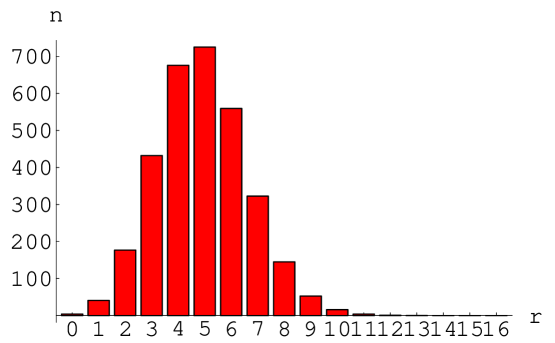
Figure 15: Distribution of total rank of gauge group over the solutions of tadpole conditions for Type IIB orientifold of quintic Gepner model.

It is interesting that the peak of the distribution lies around rank $5$, which is rather close to the value of the Standard Model. Let us also note that the distribution goes to zero very rapidly for large ranks, and — somewhat surprisingly — has a rather large support at small ranks. In particular, rank $0$, which corresponds in our language to having only distinct parity-invariant branes supporting $O(1)$ gauge groups, appears with appreciable frequency.

6.5 Solutions of the tadpole conditions — Two parameter model

Similarly to the quintic, we use the $8$ ${\bf L}={\bf 0}$ branes to express the charges of the other branes and the O-planes. The charges of these $8$ branes satisfy the two relations

$$\bigl{[}B^{B}_{(00000),0}\bigr{]}+\bigl{[}B^{B}_{(00000),4}\bigr{]}+\bigl{[}B^{B}_{(00000),8}\bigr{]}+\bigl{[}B^{B}_{(00000),12}\bigr{]} = 0$$

$$\bigl{[}B^{B}_{(00000),2}\bigr{]}+\bigl{[}B^{B}_{(00000),6}\bigr{]}+\bigl{[}B^{B}_{(00000),10}\bigr{]}+\bigl{[}B^{B}_{(00000),14}\bigr{]} = 0$$ (6.34)

For the practical computations, we will use the relations (6.34) to project to a linearly independent set of $6$ charges with the matrix

$$T=\left(\begin{array}[]{cccccccc}1&0&0&0&0&0&-1&0\\ 0&1&0&0&0&0&0&-1\\ 0&0&1&0&0&0&-1&0\\ 0&0&0&1&0&0&0&-1\\ 0&0&0&0&1&0&-1&0\\ 0&0&0&0&0&1&0&-1\\ \end{array}\right)$$ (6.35)

6.5.1 Parities and O-planes

In the two parameter model, we have various parities $P^{B}_{(\omega;\epsilon_{1},\ldots,\epsilon_{5})}$ to consider. Here $\omega=0,1$ and $(\epsilon_{1},\ldots,\epsilon_{5})$, $\epsilon_{i}=\pm$, denote the twisting by quantum and classical symmetries, respectively. This is a slightly redundant labeling because as we recall $(\epsilon_{1},\epsilon_{2},\epsilon_{3},\epsilon_{4},\epsilon_{5})$ is the same parity as $(-\epsilon_{1},-\epsilon_{2},\epsilon_{3},\epsilon_{4},\epsilon_{5})$. The charges of the corresponding O-planes are given in table 6 and table 7 in subsection 6.1.2.

6.5.2 Supersymmetry preserving branes

Even quantum symmetry

According to the discussion in subsection 6.1.2, O-planes corresponding to parities with even quantum symmetry dressing preserve a spacetime supersymmetry with even $M$-label, $M_{O}=0,8,4,12$, depending on the $\epsilon_{i}$’s. Branes preserving the same supersymmetry must have $M=M_{O}$ or $M=M_{O}+8$, and this restricts the possible ${\bf L}$ labels of the branes to $L_{1}+L-2={\rm even}$. In order to get familiar with the use of the formula (6.24), we give here a list of branes preserving the same supersymmetry as any given O-plane as well as their charges. We only list ${\bf L}$ labels up to permutation of factors with equal levels. In the last column, we give the expansion of the brane charge (for $M_{O}=0$) in terms of the ${\bf L}={\bf 0}$ branes, modulo the relations (6.34). As one can see, there are $15$ different charges. The eight-component vectors give, for example, the following equation:

$$[\widehat{B}^{B}_{{\bf\frac{k}{2}},M}]~{}=~{}\frac{1}{4}[B^{B}_{{\bf\frac{k}{2}},M}]~{}=~{}[B^{B}_{{\bf 0},M+4}]+2[B^{B}_{{\bf 0},M+2}]+2[B^{B}_{{\bf 0},M}]+2[B^{B}_{{\bf 0},M-2}]+[B^{B}_{{\bf 0},M-4}].$$ (6.36)

It is also a useful exercise to check the “multiplicity” or number of inequivalent branes with the same charge.

charge #	${\bf L}$	$M$	$S$	$g^{-M_{O}/2}Q$	multiplicity $m_{i}$
$1$	$(00000)$	$M_{O}$	$0$	$(1,0,0,0,0,0,0,0)$	$1$
$2$	$(00000)$	$M_{O}+8$	$2$	$(1,0,1,0,0,0,1,0)$	$1$
$3$	$(11000)$	$M_{O}$	$0$	$(2,1,0,0,0,0,0,1)$	$1$
$4$	$(11000)$	$M_{O}+8$	$2$	$(2,1,2,0,0,0,2,1)$	$1$
$5$	$(20000)$	$M_{O}$	$0$	$(1,1,0,0,0,0,0,1)$	$2$
$6$	$(20000)$	$M_{O}+8$	$2$	$(1,1,1,0,0,0,1,1)$	$2$
$7$	$(22000)$	$M_{O}$	$0$	$(3,2,1,0,0,0,1,2)$	$1$
$8$	$(22000)$	$M_{O}+8$	$2$	$(3,2,2,0,0,0,2,2)$	$1$
$9$	$(00100)$, $(00111)$	$M_{O}$		$(0,1,0,0,0,0,0,1)$	$4$
$10$	$(00110)$	$M_{O}$		$(1,0,\frac{1}{2},0,0,0,\frac{1}{2},0)$	$6$
$11$	$(11100)$, $(11111)$, $(31000)$, $(31110)$, $(33100)$, $(33111)$	$M_{O}$		$(2,2,1,0,0,0,1,2)$	$16$
$12$	$(11110)$, $(20100)$, $(20111)$, $(31100)$, $(31111)$, $(33000)$, $(33110)$	$M_{O}$		$(2,1,1,0,0,0,1,1)$	$38$
$13$	$(20110)$	$M_{O}$		$(1,1,\frac{1}{2},0,0,0,\frac{1}{2},1)$	$12$
$14$	$(22100)$, $(22111)$	$M_{O}$		$(4,3,2,0,0,0,2,3)$	$4$
$15$	$(22110)$	$M_{O}$		$(3,2,\frac{3}{2},0,0,0,\frac{3}{2},2)$	$6$

Odd quantum symmetry

O-planes corresponding to dressing with odd quantum symmetry preserve a spacetime supersymmetry with odd $M$-label $M=1,5,9,13$, depending on the $\epsilon_{i}$’s. We are then restricted to branes with $L_{1}+L_{2}$ odd. The list of branes and charges is

charge #	${\bf L}$	$M$	$S$	$g^{-(M_{O}-1)/2}Q$	multiplicity $m_{i}$
$1$	$(10000)$	$M_{O}$	$0$	$(1,1,0,0,0,0,0,0)$	$2$
$2$	$(10000)$	$M_{O}+8$	$2$	$(1,1,1,1,0,0,1,1)$	$2$
$3$	$(21000)$	$M_{O}$	$0$	$(2,2,1,0,0,0,0,1)$	$2$
$4$	$(21000)$	$M_{O}+8$	$2$	$(2,2,2,1,0,0,1,2)$	$2$
$5$	$(10100)$, $(10111)$ $(30000)$, $(30110)$	$M_{O}$		$(1,1,1,0,0,0,0,1)$	$16$
$6$	$(10110)$, $(30100)$ $(30111)$	$M_{O}$		$(1,1,\frac{1}{2},\frac{1}{2},0,0,\frac{1}{2},\frac{1}{2})$	$28$
$7$	$(21100)$, $(21111)$ $(32000)$, $(32110)$	$M_{O}$		$(3,3,2,1,0,0,1,2)$	$16$
$8$	$(21110)$, $(32100)$ $(32111)$	$M_{O}$		$(2,2,\frac{3}{2},\frac{1}{2},0,0,\frac{1}{2},\frac{3}{2})$	$28$

6.5.3 Action of parities on D-branes

We summarize the action of the B-type parities $P^{B}_{\omega;\epsilon_{1},\ldots,\epsilon_{5}}$ on the branes $B^{B}_{{\bf L},M,S,\psi}$ for the two parameter model $(6,6,2,2,2)$.

Neglecting again for a very short moment the $S$ and $\psi$ labels, the branes are mapped under parity as follows:

$$P^{B}_{0;\epsilon_{1}...\epsilon_{5}}:B_{{\bf L},M}\longmapsto\epsilon_{1}\cdots\epsilon_{5}B_{{\bf L},-M},$$

$$P^{B}_{1;\epsilon_{1}...\epsilon_{5}}:B_{{\bf L},M}\longmapsto\epsilon_{1}\cdots\epsilon_{5}B_{{\bf L},2-M}.$$

For branes carrying a $\psi$ label, this $\psi$ label is transformed according to

$$\psi\longmapsto(-1)^{|\bf S|/2}\;\psi.$$ (6.37)

If the sign $\epsilon_{1}\cdots\epsilon_{5}$ is negative, this means that the branes are mapped to antibranes. This minus signs can be absorbed according to the rule

$$-B_{{\bf L},M,S}=B_{{\bf L},M,S+2},~{}~{}-B_{{\bf L},M}=B_{{\bf L},M+H},~{}~{}-\widehat{B}_{{\bf L},M}^{\psi}=\widehat{B}_{{\bf L},M+H}^{-\psi}.$$ (6.38)

Restricting ourselves to the supersymmetry-preserving branes, we find that the branes with $|{\bf S}|=$ odd are all parity invariant. As for the branes with $|{\bf S}|=$ even, those with $|{\bf S}|=0$ or $4$ are invariant under parities with $\epsilon_{1}\cdots\epsilon_{5}=1$ and not under parities with $\epsilon_{1}\cdots\epsilon_{5}=-1$. The branes with $|{\bf S}|=2$ behave in an opposite way.

The gauge group on parity invariant branes is either $O$ or $Sp$ according to the sign (6.20) or (6.21). Other branes support the unitary gauge groups. A complete list of supersymmetry-preserving branes together with the gauge groups is given in tables 9, 10 in subsection 6.6.

We have presented the list of D-branes preserving the same supersymmetry as any given orientifold, and they formed 15 or 8 groups according to the RR-charge. The number of groups depends on the dressings with quantum symmetries. Each group contains branes having different signature $\sigma$ and therefore supporting different gauge groups, and it is necessary for counting the supersymmetric vacua to know the numbers $m_{i}^{\sigma}$ of branes with definite signature in a given group. They are defined to satisfy

$$m_{i}=m_{i}^{+}+2m_{i}^{0}+m_{i}^{-},$$ (6.39)

where $m_{i}$ is the total multiplicity of branes in the $i$-th group. For later convenience we give a table of these numbers below.

$\#$	$\!\!P_{0;+++++}\!\!$	$\!\!P_{0;+-+++}\!\!$	$\!\!P_{0;++-++}\!\!$	$\!\!P_{0;+--++}\!\!$	$\!\!P_{0;++--+}\!\!$	$\!\!P_{0;+---+}\!\!$	$\!\!P_{0;++---}\!\!$	$\!\!P_{0;+----}\!\!$
1,2,7,8	(1,0,0)	(0,1,0)	(0,1,0)	(0,0,1)	(0,0,1)	(0,1,0)	(0,1,0)	(1,0,0)
3,4	(1,0,0)	(0,1,0)	(0,1,0)	(1,0,0)	(0,0,1)	(0,1,0)	(0,1,0)	(0,0,1)
5,6	(2,0,0)	(0,2,0)	(0,2,0)	(0,0,2)	(0,0,2)	(0,2,0)	(0,2,0)	(2,0,0)
9,14	(3,0,1)	(0,0,4)	(2,0,2)	(1,0,3)	(3,0,1)	(2,0,2)	(0,0,4)	(1,0,3)
10,15	(0,6,0)	(0,0,6)	(4,0,2)	(0,6,0)	(0,6,0)	(2,0,4)	(6,0,0)	(0,6,0)
11	(5,0,11)	(15,0,1)	(7,0,9)	(11,0,5)	(7,0,9)	(9,0,7)	(9,0,7)	(9,0,7)
12	(6,20,12)	(20,10,8)	(12,10,16)	(10,20,8)	(12,20,6)	(16,10,12)	(8,10,20)	(8,20,10)
13	(0,12,0)	(0,0,12)	(8,0,4)	(0,12,0)	(0,12,0)	(4,0,8)	(12,0,0)	(0,12,0)

$\#$	$\!\!P_{1;+++++}\!\!$	$\!\!P_{1;+-+++}\!\!$	$\!\!P_{1;++-++}\!\!$	$\!\!P_{1;+--++}\!\!$	$\!\!P_{1;++--+}\!\!$	$\!\!P_{1;+---+}\!\!$	$\!\!P_{1;++---}\!\!$	$\!\!P_{1;+----}\!\!$
1,2,3,4	(2,0,0)	(0,2,0)	(0,2,0)	(1,0,1)	(0,0,2)	(0,2,0)	(0,2,0)	(1,0,1)
5,7	(8,0,8)	(8,0,8)	(8,0,8)	(8,0,8)	(8,0,8)	(8,0,8)	(8,0,8)	(8,0,8)
6,8	(0,24,4)	(12,4,12)	(12,4,12)	(2,24,2)	(4,24,0)	(12,4,12)	(12,4,12)	(2,24,2)

Table 8: Multiplicities $(m_{i}^{+},2m_{i}^{0},m_{i}^{-})$ of branes with different gauge groups.

6.5.4 Counting the Solutions

Let us now count the number of supersymmetric vacua in various orientifolds of two parameter model. As compared to the case with quintic, there arise a new complication due to the presence of $Sp$ or $U$-type branes. We explain the detail of the counting in the cases $P^{B}_{0,+++++}$ and $P^{B}_{0,+-+++}$, and state the results for other cases briefly.

Parity $P^{B}_{0;+++++}$

Using (6.36) and the expression in the table 6, this O-plane is shown to have the RR-charge

$$\bigl{[}O_{P}\bigr{]}~{}=~{}(2,6,16,26,30,26,16,6)^{t}~{}\simeq~{}-(28,20,14,0,0,0,14,20)^{t}.$$ (6.40)

Under the choice $\widetilde{\omega}^{\frac{1}{2}}=-1$, it preserves a spacetime supersymmetry corresponding to $M_{O}=0$. We denote by $n_{i}$, $i=1,2,\ldots,15$ the number of times a given charge appears in a tadpole canceling configuration. Computing the charges, projecting onto $6$ independent ones and equating brane and O-plane charges leads to the following three linearly independent equations on the $n_{i}$’s.

$$\left(\begin{array}[]{ccccccccccccccc}1&1&2&2&1&1&3&3&0&1&2&2&1&4&3\\ 0&0&1&1&1&1&2&2&1&0&2&1&1&3&2\\ 0&1&0&2&0&1&1&2&0&\frac{1}{2}&1&1&\frac{1}{2}&2&\frac{3}{2}\end{array}\right)\left(\begin{array}[]{c}n_{1}\\ n_{2}\\ \vdots\\ n_{15}\end{array}\right)=\left(\begin{array}[]{c}28\\ 20\\ 14\end{array}\right)$$ (6.41)

Note that again, there is a finite number of solutions to these equations, and we can count the total number of tadpole canceling D-brane configurations.

The counting goes in the following way. Suppose that the numbers $\{n_{i}\}$ ($i=1,\cdots,15$ or $8$) give a solution to (6.41). For each solution, we have to distribute the charge over the various branes with fixed charge, taking into account their signature $\sigma$. The first 8 charges are carried only by $O$-type branes, but the other 7 are carried by branes with various signatures. We note that even though the charges $i>8$ are invariant under the parity, the branes themselves need not be because of the action on the $\psi$-label. Consider all the possible decompositions of each $n_{i}$ ($i=9,\cdots,15$) into

$$n_{i}=n_{i}^{+}+n_{i}^{0}+n_{i}^{-}$$ (6.42)

with the condition that $n_{i}^{0}$ and $n_{i}^{-}$ be even. The combinatorial factor associated to a solution $\{n_{i}\}$ is given by the sum over all the possible decompositions

$$\#(n_{i})=(n_{5}+1)(n_{6}+1)\prod_{i=9}^{15}\sum_{n_{i}=\Sigma_{\sigma}n_{i}^{\sigma}}\left(\!\!\begin{array}[]{c}\frac{n_{i}^{-}}{2}+m^{-}_{i}-1\\[0.0pt] \frac{n_{i}^{-}}{2}\end{array}\!\!\right)\left(\!\!\begin{array}[]{c}\frac{n_{i}^{0}}{2}+m_{i}^{0}-1\\ \frac{n_{i}^{0}}{2}\end{array}\!\!\right)\left(\!\!\begin{array}[]{c}n_{i}^{+}+m_{i}^{+}-1\\ n_{i}^{+}\end{array}\!\!\right).$$ (6.43)

The number of vacua is therefore the sum of this over all the solutions $\{n_{i}\}$. The total number turns out to be $13213511375147\approx 10^{13}$.

Parity $P^{B}_{0;+-+++}$

Under the choice $\widetilde{\omega}^{\frac{1}{2}}=-i$, this O-plane preserves a spacetime supersymmetry corresponding to $M_{O}=4$. Its RR-charge is

$$\bigl{[}O_{P}\bigr{]}~{}=~{}(0,-4,-6,-4,0,4,6,4)^{t}~{}\simeq~{}-(6,8,12,8,6,0,0,0)^{t}.$$ (6.44)

One can easily see that the first $8$ branes on the list are mapped onto each other under this parity, and give rise to a unitary gauge group. We have to require $n_{i}=n_{i+1}$ for $i=1,3,5,7$. Equating crosscap and brane charge then leads to the two independent conditions

$$\left(\begin{array}[]{ccccccccccc}2&4&2&6&0&1&2&2&1&4&3\\ 0&2&2&4&1&0&2&1&1&3&2\end{array}\right)\left(\begin{array}[]{c}n_{1}\\ n_{3}\\ \vdots\\ n_{15}\end{array}\right)=\left(\begin{array}[]{c}12\\ 8\end{array}\right).$$ (6.45)

The number of vacua is given by the sum of the combinatoric factors

$$\#(n_{i})=\bigl{(}n_{5}+1\bigr{)}\;\prod_{i=9}^{15}\sum\left(\!\!\begin{array}[]{c}\frac{n_{i}^{-}}{2}+m^{-}_{i}-1\\[0.0pt] \frac{n_{i}^{-}}{2}\end{array}\!\!\right)\left(\!\!\begin{array}[]{c}\frac{n_{i}^{0}}{2}+m_{i}^{0}-1\\ \frac{n_{i}^{0}}{2}\end{array}\!\!\right)\left(\!\!\begin{array}[]{c}n_{i}^{+}+m_{i}^{+}-1\\ n_{i}^{+}\end{array}\!\!\right),$$ (6.46)

over all the solutions of (6.45). The total number is $47803952$.

Other parities (with even quantum symmetry dressings)

One can analyze the cases with other parities in a similar way. Let us denote by $|\epsilon|$ the number of minus signs in $\epsilon_{i}$. Choosing $\widetilde{\omega}^{\frac{1}{2}}=-i^{|\epsilon|}$ for the parity $P^{B}_{0;\epsilon_{1}\epsilon_{2}\epsilon_{3}\epsilon_{4}\epsilon_{5}}$, the O-plane preserves a spacetime supersymmetry corresponding to $M_{O}=4|\epsilon|$. The O-planes have the RR-charges

$$\bigl{[}O_{P^{B}_{0;+++++}}\bigr{]} \simeq -(28,20,14,0,0,0,14,20)^{t},$$

$$\bigl{[}O_{P^{B}_{0;+-+++}}\bigr{]}~{}=~{}\bigl{[}O_{P^{B}_{0;++-++}}\bigr{]} \simeq -(6,8,12,8,6,0,0,0)^{t},$$

$$\bigl{[}O_{P^{B}_{0;+--++}}\bigr{]}~{}=~{}\bigl{[}O_{P^{B}_{0;++--+}}\bigr{]} \simeq -(0,0,2,4,4,4,2,0)^{t},$$

$$\bigl{[}O_{P^{B}_{0;+---+}}\bigr{]}~{}=~{}\bigl{[}O_{P^{B}_{0;++---}}\bigr{]} \simeq -(2,0,0,0,2,0,4,0)^{t},$$

$$\bigl{[}O_{P^{B}_{0;+----}}\bigr{]} \simeq -(-4,4,-2,0,0,0,-2,4)^{t}.$$ (6.47)

So the tadpole cancellation conditions for other O-planes are given by the replacements $(28,20,14)\rightarrow(x,y,z)$ in (6.41), where $x,y$ and $z$ are the $(2|\epsilon|+1)$-st, $(2|\epsilon|+2)$-nd and $(2|\epsilon|+3)$-rd components of the above vectors. When $|\epsilon|$ is odd, the branes in the groups $i=1,\cdots,8$ are all U-type and the parity maps the charges $1\leftrightarrow 2$, $3\leftrightarrow 4$ and so on. So we have to put $n_{i}=n_{i+1}$ for $i={1,3,5,7}$ in these cases, and there remain only two linearly independent equations for $n_{1},n_{3},\cdots,n_{15}$.

The total number of vacua is given by the sum of combinatoric factors $\#(n_{i})$, defined in a similar way as (6.43) or (6.46), over all the solutions $\{n_{i}\}$ of tadpole cancellation condition. The result is summarized below.

$\!\!B_{0;+++++}\!\!$	$\!\!B_{0;+-+++}\!\!$	$\!\!B_{0;++-++}\!\!$	$\!\!B_{0;+--++}\!\!$	$\!\!B_{0;++--+}\!\!$	$\!\!B_{0;+---+}\!\!$	$\!\!B_{0;++---}\!\!$	$\!\!B_{0;+----}\!\!$
13213511375147	47803952	434841441	1051	2162	35	148	0

Other parities (with odd quantum symmetry dressings)

For parities $P^{B}_{1;\epsilon_{1}\epsilon_{2}\epsilon_{3}\epsilon_{4}\epsilon_{5}}$ with odd quantum symmetry dressings, we choose $\widetilde{\omega}^{\frac{1}{2}}=-i^{|\epsilon|}$ and consider the systems of an O-plane and D-branes with $M_{O}=1+4|\epsilon|$. In solving the tadpole cancellation condition, note first that for the parities $P^{B}_{+-***}$ the O-planes have no RR-charge so that the O-planes by themselves give the unique consistent superstring backgrounds. For other parities, the O-planes have the RR-charges

$$\bigl{[}O_{P^{B}_{1;+++++}}\bigr{]} \simeq -(28,28,20,8,0,0,8,20)^{t},$$

$$\bigl{[}O_{P^{B}_{1;++-++}}\bigr{]} \simeq -(4,8,12,12,8,4,0,0)^{t},$$

$$\bigl{[}O_{P^{B}_{1;++--+}}\bigr{]} \simeq -(0,0,0,4,4,4,4,0)^{t},$$

$$\bigl{[}O_{P^{B}_{1;++---}}\bigr{]} \simeq -(0,4,0,0,4,0,4,4)^{t}.$$ (6.48)

Tadpole cancellation condition is then given by three linearly independent equations on 8 numbers. For the parity $P^{B}_{1;+++++}$ it becomes

$$\left(\begin{array}[]{cccccccc}1&1&2&2&1&1&3&2\\ 0&1&1&2&1&\frac{1}{2}&2&\frac{3}{2}\\ 0&1&0&1&0&\frac{1}{2}&1&\frac{1}{2}\end{array}\right)\left(\begin{array}[]{c}n_{1}\\ n_{2}\\ \vdots\\ n_{8}\end{array}\right)~{}=~{}\left(\begin{array}[]{c}28\\ 20\\ 8\end{array}\right),$$ (6.49)

and for other parities we only have to replace the numbers $(28,20,8)$ on the right hand side with $(2|\epsilon|+2,2|\epsilon|+3,2|\epsilon|+4)$-th components of the vectors (6.48). When $|\epsilon|$ is odd, the branes in the group 1 and 2, 3 and 4 are mapped to each other. So we have to put $n_{1}=n_{2},n_{3}=n_{4}$ for such cases, and the number of independent equations on $n_{1,3,5,6,7,8}$ turns out to be reduced by one.

The total number of vacua is then calculated as a sum of a certain combinatoric factor over all the solutions $n_{i}$ of the above equations. The results are summarized below.

$\!\!B_{1;+++++}\!\!$	$\!\!B_{1;++-++}\!\!$	$\!\!B_{1;++--+}\!\!$	$\!\!B_{1;++---}\!\!$	$\!\!B_{1;+-***}\!\!$
28956442028638	1093287843	654	0	1

6.5.5 Distribution of gauge group rank

Let us see the distribution of the rank of gauge group over the supersymmetric vacua. For the brane configuration with gauge group $G=\prod O(N_{j^{+}})\times\prod U(N_{j^{0}})\times\prod Sp(N_{j^{-}})$, the rank is counted as

$$\sum_{j^{+}}\left[\frac{N_{j^{+}}}{2}\right]+\sum_{j^{0}}N_{j^{0}}+\sum_{j^{-}}N_{j^{-}}.$$

The results are summarized in the table below.

As the table shows, in the type I cases the rank of the gauge group is peaked around $9$, differently from the quintic case. Also, the number of vacua with low ranks are more strongly suppressed because of the presence of $U$ or $Sp$ type branes. For other orientifolds the maximum allowed rank is reduced, and the distributions are peaked at lower values of rank.

rank	$P_{0;+++++}$	$P_{0;+-+++}$	$P_{0;++-++}$	$P_{0;+--++}$	$P_{0;++--+}$	$P_{0;+---+}$	$P_{0;++---}$
	13213511375147	47803952	434841441	1051	2162	35	148
0	646540	508725	4926687	166	480	0	15
1	44771470	2554170	29783246	330	721	7	105
2	1031791551	7173709	76613078	397	719	28	28
3	11643923756	11188898	113881856	88	172
4	75080785790	11195422	102828964	70	70
5	302754231919	8532104	66661000
6	816375589073	4126724	28541380
7	1555478380691	1860600	9347940
8	2202010164391	501900	1980090
9	2424675084374	129360	244860
10	2159636846181	32340	32340
11	1607633137394
12	1023393658328
13	567624907070
14	277143210040
15	120183191993
16	46373508969
17	15919273033
18	4851273490
19	1288731061
20	300818948
21	56875115
22	9505650
23	961928
24	106392

rank	$P_{1;+++++}$	$P_{1;++-++}$	$P_{1;++--+}$
	28956442028638	1093287843	654
0	131418	10073409	70
1	12060448	98476432	448
2	355100152	281607952	136
3	5191991568	398177360
4	44410530386	248315690
5	245511738472	52357760
6	928376315288	4279240
7	2485035106608
8	4801648669394
9	6693313716784
10	6689330341632
11	4555609978656
12	2009612464368
13	457636777344
14	40397106120

6.6 Particle Spectrum in Some Supersymmetric Models

A closer look at the annulus and the Möbius strip amplitudes gives us a more detailed information on the spectrum of open strings. Let us now turn to count the number of matter fields between the same branes. There are many branes and each has quite a few scalar fields, so the best way to count them is again to use computers. As in the analysis of A-branes, the massless chiral fields in the spacetime theory are in one to one correspondence with the chiral primary states in the internal theory. Let us summarize the necessary materials.

• The open string NS state $\otimes_{i}(l_{i},n_{i},s_{i})$ between the branes $B^{B}_{{\bf L},M}$ and $B^{B}_{{\bf L}^{\prime},M^{\prime}}$ obey $\sum_{i}n_{i}w_{i}=M^{\prime}-M~{}({\rm mod}~{}2H)$, as well as the usual selection rule $l_{i}+n_{i}\in 2{\mathbb{Z}}$ and the $SU(2)$ fusion rule constraint. The states between short-orbit branes with the same $\bf S$ and additional labels $\psi,\psi^{\prime}=\pm 1$ are subject to a projection $\prod_{i\in{\bf S}}(-1)^{\frac{1}{2}(l_{i}+n_{i})}=\psi\psi^{\prime}$.

• The open string states on parity-invariant D-branes have definite eigenvalues of parity. The Möbius strip amplitude between $B_{{\bf L},M}$ and its image under $P^{B}_{M_{\omega};\epsilon_{i}}$ contains NS states $\otimes_{i}(l_{i},2\nu_{i},s_{i})$ satisfying $\sum_{i}\nu_{i}w_{i}=M_{\omega}-M$ (mod $H$), as well as the $SU(2)$ fusion constraint on $l_{i}$. The contribution of massless states to Möbius strip amplitude is given by the sum of chiral primary states satisfying these condition, with the phase

  $$i^{-1+|\epsilon|+\{\#{\rm of}(s_{i}=2)\}}\prod_{i}\epsilon_{i}^{L_{i}+\nu_{i}}.$$

We present here the relevant amplitudes from which the result follows. The annulus amplitudes between two long-orbit B-branes $B^{B}_{{\bf L},M}$ and $B^{B}_{{\bf L}^{\prime},M^{\prime}}$ has the following NS part:

$$\langle B^{B}_{{\bf L},M}|q^{H}|B^{B}_{{\bf L}^{\prime},M^{\prime}}\rangle|_{{{}_{\rm NS}}}$$ (6.50)

$$= \frac{1}{2}\sum_{n_{i}}\delta^{(2H)}_{\sum_{i}w_{i}n_{i}+M-M^{\prime}}\sum_{l_{i}}\prod_{i=1}^{r}N_{L_{i}L^{\prime}_{i}}^{~{}l_{i}}\times\left\{\chi^{(\rm st)NS+}\prod_{i=1}^{r}\chi^{\rm NS+}_{l_{i},n_{i}}-\chi^{(\rm st)NS-}\prod_{i=1}^{r}\chi^{\rm NS-}_{l_{i},n_{i}}\right\}$$

Here $\chi^{(\rm st)NS\pm}$ and $\chi^{\rm NS\pm}_{l,n}=\chi_{l,n,0}\pm\chi_{l,n,2}$ are the same as those used in the discussion of A-branes. The delta symbol represents that the sum over $n_{i}$ is taken over the $\widetilde{\Gamma}$-orbit but is shifted by $M$ and $M^{\prime}$. For two short-orbit branes $\widehat{B}^{B}_{{\bf L},M}$ and $\widehat{B}^{B}_{{\bf L}^{\prime},M^{\prime}}$ the above amplitude has to be divided by $2^{[|{\bf S}|/2]}2^{[|{\bf S}^{\prime}|/2]}$, where ${\bf S}$ and ${\bf S}^{\prime}$ are the sets of $i$’s such that $L_{i}$ or $L^{\prime}_{i}$ coincide with $\frac{k_{i}}{2}$. When ${\bf S}={\bf S}^{\prime}$ and $|{\bf S}|=2$ or $4$, the twisted parts of boundary states yield

$$\pm\frac{1}{2^{1+|{\bf S}|}}\sum_{n_{i}}\delta^{(2H)}_{\sum_{i}w_{i}n_{i}+M-M^{\prime}}\sum_{l_{i}}\prod_{i=1}^{r}N_{L_{i}L^{\prime}_{i}}^{~{}l_{i}}\times\prod_{i\in{\bf S}}(-1)^{\frac{1}{2}(l_{i}+n_{i})}$$

$$\hskip 56.9055pt\times\left\{\chi^{(\rm st)NS+}\prod_{i=1}^{r}\chi^{\rm NS+}_{l_{i},n_{i}}-\chi^{(\rm st)NS-}\prod_{i=1}^{r}\chi^{\rm NS-}_{l_{i},n_{i}}\right\},$$ (6.51)

so the states with $\prod_{i\in{\bf S}}(-1)^{\frac{1}{2}(l_{i}+n_{i})}=1\,(-1)$ propagates between the branes with the same (opposite) signs. All these maintain the integrality of the open string spectrum, and ensure that every single B-brane supports a $U(1)$ gauge symmetry in the absence of orientifolds.

For parity-invariant branes, we have to find the action of parity on the matter fields on their worldvolume. The NS part of Möbius strip amplitude between a long-orbit B-brane $B^{B}_{{\bf L},M}$ and its image under the parity $P^{B}_{\omega,{\bf m}}$ reads (recall $\omega=\,{\rm e}^{\frac{2\pi iM_{\omega}}{H}}$ and $\widetilde{\omega}_{i}=\,{\rm e}^{-\frac{2\pi im_{i}}{k_{i}+2}}=\pm 1$)

$$\langle B^{B}_{{\bf L},M}|q^{H}|C^{B}_{\omega,{\bf m}}\rangle|_{{{}_{\rm NS}}}$$ (6.52)

$$= {\rm Re}\left\{i\,{\rm e}^{\frac{\pi i(r-d)}{4}}\widetilde{\omega}^{{\bf L}-\frac{1}{2}}\sum_{\widetilde{\nu}_{i}\in{\mathbb{Z}}_{k_{i}+2}}\delta^{(1)}_{\sum_{i}\frac{\widetilde{\nu}_{i}}{k_{i}+2},\frac{M_{\omega}-M}{H}}\sum_{l_{i}}\widetilde{\omega}^{\widetilde{\nu}}\hat{\chi}^{(\rm st)NS+}\prod_{i=1}^{r}N_{L_{i}L_{i}}^{~{}l_{i}}\hat{\chi}^{\rm NS+}_{l_{i},2\widetilde{\nu}_{i}}\right\}$$

where the characters $\hat{\chi}^{(\rm st)NS\pm}$, $\hat{\chi}^{\rm NS\pm}_{l,n}$ are the same as those appeared in the discussion of A-branes. The expressions are the same for short-orbit branes except for obvious change of normalizations. The states contributing to the above Möbius strip amplitude with $+(-)$ signs are the eigenstates of the parity with eigenvalues $P^{B}_{\omega;{\bf m}}=+1(-1)$. We also see that, in the $q_{l}$-expansion of this amplitude, the terms of order $q_{l}^{0}$ corresponding to gauge fields appear with the sign $-\epsilon^{\omega;{\bf m}}_{{\bf L},M}$.

6.6.1 Quintic

For the quintic, there exists only a single parity of interest. We are considering supersymmetry preserving branes, which in the case of the quintic are invariant under the parity. The following table lists the number of massless scalars on these branes and their transformation properties under parity: $(n_{1},n_{2})$ denotes the number of (symmetric, antisymmetric) massless scalars.

($L_{i}$)	$(n_{1},n_{2})$
(00000)	$(0,0)$
(10000)	$(4,0)$
(11000)	$(8,3)$
(11100)	$(15,9)$
(11110)	$(28,22)$
(11111)	$(51,50)$

It is now straightforward to find the matter content of supersymmetric tadpole canceling configurations. Two such solutions have been given in [36], the standard solution with $4$ branes of type $(11111)$ and the one with $12$ branes of type $(00000)$ and $20$ of type $(10000)$, which is the configuration with the highest possible rank in this example. Just for the purposes of illustration, we give a third configuration, which is chosen completely randomly. We consider a setup consisting of $4$ branes of type $(11000)$ and $8$ of $(00111)$. The matter content under the gauge group $O(4)\times O(8)$ is

$$8({\bf 10},{\bf 1})\oplus 3({\bf 6},\bf{1})\oplus 15({\bf 1},{\bf 36})\oplus 9({\bf 1},{\bf 28})\oplus 101({\bf 4},{\bf 8}).$$ (6.53)

The part of the spectrum involving only one type of brane can be directly read off from the above table. For those strings that connect one type of brane to another, note that there is always a linear combination of any open string operator and its parity image that survives the projection. As a consequence,this part of the spectrum can be determined using the results on the open string spectrum without orientifolds.

6.6.2 Two parameter model

The tables 9 and 10 list the gauge groups $G$ and the number of matters on the D-branes for various choices of orientifolds of the two parameter model. For $G=O$ or $Sp$, the two numbers in $G_{(n_{1},n_{2})}$ mean there are massless scalars in $n_{1}$ symmetric and $n_{2}$ antisymmetric tensor representations of $G$. For $G=U$ the three numbers in $U_{(n_{1},n_{2},n_{3})}$ mean there are $n_{1}$ adjoint, $n_{2}$ symmetric tensor and $n_{3}$ antisymmetric tensor representations.

($L_{i}$)	$P_{0;+++++}$	$P_{0;++-++}$	$P_{0;++++-}$	$P_{0;++--+}$	$P_{0;+++--}$	$P_{0;++---}$
(00000)	$O_{(0,0)}$	$U_{(0,2,1)}$	$U_{(0,2,1)}$	$Sp_{(0,0)}$	$Sp_{(0,0)}$	$U_{(0,3,0)}$
(00100)	$O_{(2,1)}$	$O_{(1,2)}$	$Sp_{(2,1)}$	$O_{(2,1)}$	$Sp_{(3,0)}$	$Sp_{(0,3)}$
(00110)	$U_{(2,1,0)}$	$O_{(1,1)}$	$Sp_{(2,0)}$	$U_{(2,0,1)}$	$U_{(2,0,1)}$	$O_{(2,0)}$
(00111)	$Sp_{(3,0)}$	$O_{(1,2)}$	$O_{(1,2)}$	$O_{(2,1)}$	$O_{(2,1)}$	$Sp_{(0,3)}$
(11000)	$O_{(5,0)}$	$U_{(5,4,6)}$	$U_{(5,4,6)}$	$Sp_{(2,3)}$	$Sp_{(2,3)}$	$U_{(5,4,6)}$
(11100)	$O_{(9,6)}$	$O_{(11,4)}$	$Sp_{(6,9)}$	$O_{(7,8)}$	$Sp_{(6,9)}$	$Sp_{(8,7)}$
(11110)	$U_{(9,3,3)}$	$O_{(6,3)}$	$Sp_{(3,6)}$	$U_{(9,5,1)}$	$U_{(9,3,3)}$	$O_{(4,5)}$
(11111)	$Sp_{(6,9)}$	$O_{(9,6)}$	$O_{(9,6)}$	$O_{(9,6)}$	$O_{(9,6)}$	$Sp_{(10,5)}$
(20000)	$O_{(4,0)}$	$U_{(4,3,4)}$	$U_{(4,3,4)}$	$Sp_{(2,2)}$	$Sp_{(2,2)}$	$U_{(4,4,3)}$
(20100)	$O_{(7,4)}$	$O_{(8,3)}$	$Sp_{(5,6)}$	$O_{(5,6)}$	$Sp_{(6,5)}$	$Sp_{(5,6)}$
(20110)	$U_{(6,3,2)}$	$O_{(4,2)}$	$Sp_{(3,3)}$	$U_{(6,4,1)}$	$U_{(6,2,3)}$	$O_{(3,3)}$
(20111)	$Sp_{(6,5)}$	$O_{(6,5)}$	$O_{(6,5)}$	$O_{(7,4)}$	$O_{(7,4)}$	$Sp_{(7,4)}$
(22000)	$O_{(13,3)}$	$U_{(16,7,12)}$	$U_{(16,7,12)}$	$Sp_{(7,9)}$	$Sp_{(7,9)}$	$U_{(16,6,13)}$
(22100)	$O_{(20,15)}$	$O_{(25,10)}$	$Sp_{(14,21)}$	$O_{(16,19)}$	$Sp_{(13,22)}$	$Sp_{(20,15)}$
(22110)	$U_{(18,8,9)}$	$O_{(12,6)}$	$Sp_{(5,13)}$	$U_{(18,13,4)}$	$U_{(18,9,8)}$	$O_{(7,11)}$
(22111)	$Sp_{(13,22)}$	$O_{(21,14)}$	$O_{(21,14)}$	$O_{(20,15)}$	$O_{(20,15)}$	$Sp_{(24,11)}$
(31000)	$O_{(9,6)}$	$Sp_{(6,9)}$	$Sp_{(6,9)}$	$Sp_{(6,9)}$	$Sp_{(6,9)}$	$O_{(5,10)}$
(31100)	$U_{(9,3,3)}$	$O_{(6,3)}$	$Sp_{(3,6)}$	$U_{(9,3,3)}$	$U_{(9,1,5)}$	$Sp_{(5,4)}$
(31110)	$Sp_{(6,9)}$	$O_{(9,6)}$	$Sp_{(4,11)}$	$O_{(9,6)}$	$Sp_{(8,7)}$	$O_{(7,8)}$
(31111)	$Sp_{(0,5)}$	$U_{(5,6,4)}$	$U_{(5,6,4)}$	$O_{(3,2)}$	$O_{(3,2)}$	$U_{(5,6,4)}$
(33000)	$U_{(9,3,3)}$	$Sp_{(3,6)}$	$Sp_{(3,6)}$	$U_{(9,1,5)}$	$U_{(9,1,5)}$	$O_{(0,9)}$
(33100)	$Sp_{(6,9)}$	$O_{(9,6)}$	$Sp_{(4,11)}$	$Sp_{(8,7)}$	$O_{(1,14)}$	$Sp_{(10,5)}$
(33110)	$Sp_{(0,5)}$	$U_{(5,6,4)}$	$U_{(5,0,10)}$	$O_{(3,2)}$	$Sp_{(4,1)}$	$U_{(5,4,6)}$
(33111)	$Sp_{(0,15)}$	$Sp_{(10,5)}$	$Sp_{(10,5)}$	$O_{(7,8)}$	$O_{(7,8)}$	$O_{(9,6)}$

($L_{i}$)	$P_{1;+++++}$	$P_{1;++-++}$	$P_{1;++++-}$	$P_{1;++--+}$	$P_{1;+++--}$	$P_{1;++---}$
(10000)	$O_{(1,0)}$	$U_{(1,3,3)}$	$U_{(1,3,3)}$	$Sp_{(0,1)}$	$Sp_{(0,1)}$	$U_{(1,3,3)}$
(10100)	$O_{(4,3)}$	$O_{(4,3)}$	$Sp_{(3,4)}$	$O_{(4,3)}$	$Sp_{(3,4)}$	$Sp_{(3,4)}$
(10110)	$U_{(5,1,1)}$	$O_{(3,2)}$	$Sp_{(2,3)}$	$U_{(5,1,1)}$	$U_{(5,1,1)}$	$O_{(3,2)}$
(10111)	$Sp_{(3,4)}$	$O_{(4,3)}$	$O_{(4,3)}$	$O_{(4,3)}$	$O_{(4,3)}$	$Sp_{(3,4)}$
(21000)	$O_{(9,0)}$	$U_{(9,5,9)}$	$U_{(9,5,9)}$	$Sp_{(4,5)}$	$Sp_{(4,5)}$	$U_{(9,5,9)}$
(21100)	$O_{(14,9)}$	$O_{(18,5)}$	$Sp_{(9,14)}$	$O_{(10,13)}$	$Sp_{(9,14)}$	$Sp_{(13,10)}$
(21110)	$U_{(13,5,5)}$	$O_{(9,4)}$	$Sp_{(4,9)}$	$U_{(13,9,1)}$	$U_{(13,5,5)}$	$O_{(5,8)}$
(21111)	$Sp_{(9,14)}$	$O_{(14,9)}$	$O_{(14,9)}$	$O_{(14,9)}$	$O_{(14,9)}$	$Sp_{(17,6)}$
(30000)	$O_{(4,3)}$	$Sp_{(3,4)}$	$Sp_{(3,4)}$	$Sp_{(3,4)}$	$Sp_{(3,4)}$	$O_{(4,3)}$
(30100)	$U_{(5,1,1)}$	$O_{(3,2)}$	$Sp_{(2,3)}$	$U_{(5,1,1)}$	$U_{(5,1,1)}$	$Sp_{(2,3)}$
(30110)	$Sp_{(3,4)}$	$O_{(4,3)}$	$Sp_{(3,4)}$	$O_{(4,3)}$	$Sp_{(3,4)}$	$O_{(4,3)}$
(30111)	$Sp_{(0,1)}$	$U_{(1,3,3)}$	$U_{(1,3,3)}$	$O_{(1,0)}$	$O_{(1,0)}$	$U_{(1,3,3)}$
(32000)	$O_{(14,9)}$	$Sp_{(9,14)}$	$Sp_{(9,14)}$	$Sp_{(9,14)}$	$Sp_{(9,14)}$	$O_{(6,17)}$
(32100)	$U_{(13,5,5)}$	$O_{(9,4)}$	$Sp_{(4,9)}$	$U_{(13,5,5)}$	$U_{(13,1,9)}$	$Sp_{(8,5)}$
(32110)	$Sp_{(9,14)}$	$O_{(14,9)}$	$Sp_{(5,18)}$	$O_{(14,9)}$	$Sp_{(13,10)}$	$O_{(10,13)}$
(32111)	$Sp_{(0,9)}$	$U_{(9,9,5)}$	$U_{(9,9,5)}$	$O_{(5,4)}$	$O_{(5,4)}$	$U_{(9,9,5)}$

Table 9: Gauge group and number of massless scalar fields

($L_{i}$)	$P_{0;+-+++}$	$P_{0;+--++}$	$P_{0;+-++-}$	$P_{0;+---+}$	$P_{0;+-+--}$	$P_{0;+----}$
(00000)	$U_{(0,0,3)}$	$Sp_{(0,0)}$	$Sp_{(0,0)}$	$U_{(0,1,2)}$	$U_{(0,1,2)}$	$O_{(0,0)}$
(00100)	$Sp_{(0,3)}$	$O_{(0,3)}$	$Sp_{(1,2)}$	$Sp_{(2,1)}$	$O_{(1,2)}$	$Sp_{(1,2)}$
(00110)	$Sp_{(0,2)}$	$U_{(2,0,1)}$	$U_{(2,0,1)}$	$O_{(0,2)}$	$Sp_{(1,1)}$	$U_{(2,1,0)}$
(00111)	$Sp_{(0,3)}$	$Sp_{(1,2)}$	$Sp_{(1,2)}$	$O_{(1,2)}$	$O_{(1,2)}$	$O_{(0,3)}$
(11000)	$U_{(5,10,0)}$	$O_{(1,4)}$	$O_{(1,4)}$	$U_{(5,6,4)}$	$U_{(5,6,4)}$	$Sp_{(2,3)}$
(11100)	$O_{(11,4)}$	$Sp_{(14,1)}$	$O_{(7,8)}$	$O_{(5,10)}$	$Sp_{(8,7)}$	$O_{(9,6)}$
(11110)	$O_{(6,3)}$	$U_{(9,5,1)}$	$U_{(9,3,3)}$	$Sp_{(9,0)}$	$O_{(4,5)}$	$U_{(9,1,5)}$
(11111)	$O_{(9,6)}$	$O_{(9,6)}$	$O_{(9,6)}$	$Sp_{(10,5)}$	$Sp_{(10,5)}$	$Sp_{(14,1)}$
(20000)	$U_{(4,1,6)}$	$Sp_{(2,2)}$	$Sp_{(2,2)}$	$U_{(4,2,5)}$	$U_{(4,2,5)}$	$O_{(0,4)}$
(20100)	$Sp_{(3,8)}$	$O_{(3,8)}$	$Sp_{(4,7)}$	$Sp_{(7,4)}$	$O_{(2,9)}$	$Sp_{(6,5)}$
(20110)	$Sp_{(1,5)}$	$U_{(6,2,3)}$	$U_{(6,0,5)}$	$O_{(1,5)}$	$Sp_{(4,2)}$	$U_{(6,3,2)}$
(20111)	$Sp_{(1,10)}$	$Sp_{(6,5)}$	$Sp_{(6,5)}$	$O_{(4,7)}$	$O_{(4,7)}$	$O_{(3,8)}$
(22000)	$U_{(16,9,10)}$	$Sp_{(7,9)}$	$Sp_{(7,9)}$	$U_{(16,8,11)}$	$U_{(16,8,11)}$	$O_{(5,11)}$
(22100)	$Sp_{(16,19)}$	$O_{(18,17)}$	$Sp_{(15,20)}$	$Sp_{(18,17)}$	$O_{(13,22)}$	$Sp_{(19,16)}$
(22110)	$Sp_{(7,11)}$	$U_{(18,9,8)}$	$U_{(18,5,12)}$	$O_{(9,9)}$	$Sp_{(10,8)}$	$U_{(18,8,9)}$
(22111)	$Sp_{(12,23)}$	$Sp_{(19,16)}$	$Sp_{(19,16)}$	$O_{(17,18)}$	$O_{(17,18)}$	$O_{(18,17)}$
(31000)	$O_{(11,4)}$	$O_{(7,8)}$	$O_{(7,8)}$	$Sp_{(8,7)}$	$Sp_{(8,7)}$	$Sp_{(8,7)}$
(31100)	$O_{(6,3)}$	$U_{(9,5,1)}$	$U_{(9,3,3)}$	$O_{(4,5)}$	$Sp_{(5,4)}$	$U_{(9,3,3)}$
(31110)	$O_{(9,6)}$	$O_{(9,6)}$	$Sp_{(8,7)}$	$Sp_{(10,5)}$	$O_{(7,8)}$	$O_{(7,8)}$
(31111)	$U_{(5,6,4)}$	$O_{(3,2)}$	$O_{(3,2)}$	$U_{(5,6,4)}$	$U_{(5,6,4)}$	$Sp_{(4,1)}$
(33000)	$O_{(6,3)}$	$U_{(9,3,3)}$	$U_{(9,3,3)}$	$Sp_{(5,4)}$	$Sp_{(5,4)}$	$U_{(9,5,1)}$
(33100)	$O_{(9,6)}$	$O_{(9,6)}$	$Sp_{(8,7)}$	$O_{(7,8)}$	$Sp_{(10,5)}$	$Sp_{(6,9)}$
(33110)	$U_{(5,6,4)}$	$O_{(3,2)}$	$Sp_{(4,1)}$	$U_{(5,6,4)}$	$U_{(5,4,6)}$	$O_{(3,2)}$
(33111)	$Sp_{(10,5)}$	$O_{(7,8)}$	$O_{(7,8)}$	$O_{(9,6)}$	$O_{(9,6)}$	$Sp_{(8,7)}$

($L_{i}$)	$P_{1;+-+++}$	$P_{1;+--++}$	$P_{1;+-++-}$	$P_{1;+---+}$	$P_{1;+-+--}$	$P_{1;+----}$
(10000)	$U_{(1,0,6)}$	$Sp_{(1,0)}$	$Sp_{(1,0)}$	$U_{(1,2,4)}$	$U_{(1,2,4)}$	$O_{(0,1)}$
(10100)	$Sp_{(1,6)}$	$O_{(0,7)}$	$Sp_{(3,4)}$	$Sp_{(5,2)}$	$O_{(2,5)}$	$Sp_{(3,4)}$
(10110)	$Sp_{(1,4)}$	$U_{(5,0,2)}$	$U_{(5,0,2)}$	$O_{(0,5)}$	$Sp_{(3,2)}$	$U_{(5,2,0)}$
(10111)	$Sp_{(1,6)}$	$Sp_{(3,4)}$	$Sp_{(3,4)}$	$O_{(2,5)}$	$O_{(2,5)}$	$O_{(0,7)}$
(21000)	$U_{(9,10,4)}$	$O_{(4,5)}$	$O_{(4,5)}$	$U_{(9,8,6)}$	$U_{(9,8,6)}$	$Sp_{(5,4)}$
(21100)	$O_{(14,9)}$	$Sp_{(15,8)}$	$O_{(12,11)}$	$O_{(10,13)}$	$Sp_{(13,10)}$	$O_{(12,11)}$
(21110)	$O_{(8,5)}$	$U_{(13,6,4)}$	$U_{(13,6,4)}$	$Sp_{(9,4)}$	$O_{(6,7)}$	$U_{(13,4,6)}$
(21111)	$O_{(14,9)}$	$O_{(12,11)}$	$O_{(12,11)}$	$Sp_{(13,10)}$	$Sp_{(13,10)}$	$Sp_{(15,8)}$
(30000)	$Sp_{(1,6)}$	$Sp_{(3,4)}$	$Sp_{(3,4)}$	$O_{(2,5)}$	$O_{(2,5)}$	$O_{(0,7)}$
(30100)	$Sp_{(1,4)}$	$U_{(5,0,2)}$	$U_{(5,0,2)}$	$Sp_{(3,2)}$	$O_{(0,5)}$	$U_{(5,2,0)}$
(30110)	$Sp_{(1,6)}$	$Sp_{(3,4)}$	$O_{(0,7)}$	$O_{(2,5)}$	$Sp_{(5,2)}$	$Sp_{(3,4)}$
(30111)	$U_{(1,0,6)}$	$Sp_{(1,0)}$	$Sp_{(1,0)}$	$U_{(1,2,4)}$	$U_{(1,2,4)}$	$O_{(0,1)}$
(32000)	$Sp_{(9,14)}$	$Sp_{(11,12)}$	$Sp_{(11,12)}$	$O_{(10,13)}$	$O_{(10,13)}$	$O_{(8,15)}$
(32100)	$Sp_{(5,8)}$	$U_{(13,4,6)}$	$U_{(13,4,6)}$	$Sp_{(7,6)}$	$O_{(4,9)}$	$U_{(13,6,4)}$
(32110)	$Sp_{(9,14)}$	$Sp_{(11,12)}$	$O_{(8,15)}$	$O_{(10,13)}$	$Sp_{(13,10)}$	$Sp_{(11,12)}$
(32111)	$U_{(9,4,10)}$	$Sp_{(5,4)}$	$Sp_{(5,4)}$	$U_{(9,6,8)}$	$U_{(9,6,8)}$	$O_{(4,5)}$

Table 10: Gauge group and number of massless scalar fields (continued)

Note that the symmetric and antisymmetric tensors of $U(n)$ are complex representations, and are supported on strings between a $U$-type brane and its parity image. The analysis of the spectrum also shows that all the $U$-type branes in the tables support equal number of (anti)symmetric tensors and their conjugates, namely, all of them support non-chiral matters. We will extend this observation later and show the non-chirality of the spectrum for general supersymmetric brane configurations in any type IIB orientifolds of Gepner model.

6.6.3 Spectrum in Sample Examples

It is straightforward to determine the matter contents in sample tadpole canceling configurations. Let us consider a few examples as an exercise.

As the first example, let us take the parity $P^{B}_{0;+++++}$ and take six branes from the group $\#14$ and two from $\#12$ to cancel the tadpole. There are still many ways to do so. For example, there are the following two inequivalent configurations supporting $O(6)\times O(2)$ gauge group:

$$6(22100)+2(20100) : 20({\bf 21,1})\oplus 15({\bf 15,1})\oplus 7({\bf 1,3})\oplus 4({\bf 1,1})\oplus 12({\bf 6,2}),$$

$$6(22100)+2(20010) : 20({\bf 21,1})\oplus 15({\bf 15,1})\oplus 7({\bf 1,3})\oplus 4({\bf 1,1})\oplus 6({\bf 6,2}).$$ (6.54)

Here ${\bf 2}$ and ${\bf 3}$ of $O(2)$ mean the reducible representations ${\bf[1]\oplus[-1]}$ and ${\bf[2]\oplus[0]\oplus[-2]}$ of $U(1)$. The configurations supporting $O(6)\times U(1)$ are

$$6(22100)+(11110)^{+}+(11110)^{-} : 20({\bf 21})\oplus 15({\bf 15})\oplus 9({\bf 1})\oplus 3({\bf 1})^{\pm\pm}\oplus 8({\bf 6})^{\pm}$$

$$6(22100)+(11011)^{+}+(11011)^{-} : 20({\bf 21})\oplus 15({\bf 15})\oplus 9({\bf 1})\oplus 3({\bf 1})^{\pm\pm}\oplus 2({\bf 6})^{\pm}$$

$$6(22100)+(31100)^{+}+(31100)^{-} : 20({\bf 21})\oplus 15({\bf 15})\oplus 9({\bf 1})\oplus 3({\bf 1})^{\pm\pm}\oplus 12({\bf 6})^{\pm}$$

$$6(22100)+(31010)^{+}+(31010)^{-} : 20({\bf 21})\oplus 15({\bf 15})\oplus 9({\bf 1})\oplus 3({\bf 1})^{\pm\pm}\oplus 6({\bf 6})^{\pm}$$

$$6(22100)+(33000)^{+}+(33000)^{-} : 20({\bf 21})\oplus 15({\bf 15})\oplus 9({\bf 1})\oplus 3({\bf 1})^{\pm\pm}\oplus 10({\bf 6})^{\pm}$$ (6.55)

Here the $\pm$ signs represent $U(1)$ charge. $18({\bf 1})$ are neutral scalars corresponding to open strings with both ends on the same short-orbit brane, while $({\bf 1})^{\pm\pm}$ correspond to strings stretching between a short-orbit brane and its parity image. There are six configurations supporting $O(6)\times Sp(1)$:

$$6(22100)+2(20111) : 20({\bf 21,1})\oplus 15({\bf 15,1})\oplus 6({\bf 1,3})\oplus 5({\bf 1,1})\oplus 6({\bf 6,2})$$

$$6(22100)+2(31111) : 20({\bf 21,1})\oplus 15({\bf 15,1})\oplus 5({\bf 1,1})\oplus 6({\bf 6,2})$$

$$6(22100)+2(33110)^{\pm} : 20({\bf 21,1})\oplus 15({\bf 15,1})\oplus 5({\bf 1,1})\oplus 10({\bf 6,2})$$

$$6(22100)+2(33011)^{\pm} : 20({\bf 21,1})\oplus 15({\bf 15,1})\oplus 5({\bf 1,1})\oplus 4({\bf 6,2})$$ (6.56)

There are indeed a lot more tadpole-canceling configurations with various choices of orientifold and D-branes, and the spectrum of massless states can be obtained in the same way.

6.7 Chirality — Vanishing Theorem

As was explained before, chirality of the theory is measured by the Witten index. Given a tadpole-free set of an O-plane and D-branes, the theory is chiral if there is a pair of D-branes with nonzero open string Witten index, or any D-brane and its parity image with nonzero twisted Witten index.

The index between two long-orbit B-branes in Gepner model can be easily computed as the diagonal elements of the following polynomial of the $H$-dimensional shift matrix $g$,

$$Q_{{\bf L},M}(g)Q_{{\bf L}^{\prime},M^{\prime}}(g^{-1})\prod_{i=1}^{r}(1-g^{w_{i}}),$$ (6.57)

where $Q_{{\bf L},M}(g)$ is the polynomial defined in (6.24). The parity twisted Witten index is given by replacing one of the two polynomials with the one representing the O-plane charge, which are given in (6.47) and (6.48).

Using the index formula (6.57), one can show that any tadpole-free configurations of an O-plane and long-orbit D-branes are non-chiral. To do this, notice first that the polynomial $Q_{{\bf L},M}(g)$ is symmetric under $g^{i}\rightarrow g^{M-i}$. Similarly, the polynomials representing the O-plane charges are symmetric under $g^{i}\rightarrow g^{M_{O}-i}$, where $M_{O}=M_{\omega}+4|\epsilon|$ characterize the spacetime supersymmetry preserved by the O-planes. On the other hand, under the assumption $\sum_{i}w_{i}=H$ the last factor in (6.57) is transformed to $(-1)^{r}$ times itself under $g\rightarrow g^{-1}$. Using all these one finds that, in standard four-dimensional models with $r=5$, the polynomial (6.57) has no $g^{0}$ term for any susy-preserving pairs of long-orbit D-branes and the O-plane. Thus the index vanishes for all such pairs.

There is still a possibility of having chiral models with B-type orientifolds of Gepner models. The point is that, in some Gepner models with even $H$, there are RR-charges carried by some short-orbit B-branes and none of long-orbit B-branes. In general, the number of RR-charges in type IIB orientifolds is $2h_{1,1}+2$, and the number of RR-charges carried by B-branes is fewer than this:

$$2h_{1,1}+2 \geq \#\mbox{(charges carried by all the short- and long-orbit B-branes)}$$ (6.58)

$$\geq \#\mbox{(charges carried by $L_{i}=0$ B-branes)}.$$

The first inequality shows that there can be RR-charges carried by none of rational B-type boundary states constructed in this paper. It is expected that such RR-charges are associated with non-toric blowups, as there are non-polynomial deformations in the IIA case. In the $k=(66222)$ model both of the above equalities hold, so there is no chiral brane configurations.

As an example where neither of the two equalities hold, let us consider the $k=(22444)$ model which is known to have $h_{1,1}=6$. Let us first work out the $14=2h_{1,1}+2$ RR ground states. First, take the RR ground states $|0\rangle_{\nu}$ ($\nu=1,\cdots,k+1$) in the level $k$ minimal model

$$|0\rangle_{\nu}=|\nu-1,\nu,1\rangle\times|\nu-1,\nu,1\rangle,$$ (6.59)

and construct the ground states of the form $|0\rangle_{(\nu_{i})}=\prod_{i}|0\rangle_{\nu_{i}}$, with $\nu_{i}=\nu$ (mod $k_{i}+2$) for all $i$. There are only eight such states:

$$|0\rangle_{(11111)},~{}~{}|0\rangle_{(22222)},~{}~{}|0\rangle_{(33333)},~{}~{}|0\rangle_{(33111)},$$

$$|0\rangle_{(11555)},~{}~{}|0\rangle_{(11333)},~{}~{}|0\rangle_{(22444)},~{}~{}|0\rangle_{(33555)}.$$ (6.60)

Other states are obtained by looking for mixed products of $|0\rangle_{\nu}$ and $|l\rangle_{{}_{\rm RR}}$, where

$$|l\rangle_{{}_{\rm RR}}=|l,l+1,1\rangle\times|l,-l-1,-1\rangle.$$ (6.61)

One finds six additional states of the form $|l_{1},l_{2}\rangle_{{}_{\rm RR}}\times|0\rangle_{(\nu_{3}\nu_{4}\nu_{5})}$:

$$|2,0\rangle_{{}_{\rm RR}}|0\rangle_{(222)},~{}~{}|1,1\rangle_{{}_{\rm RR}}|0\rangle_{(222)},~{}~{}|0,2\rangle_{{}_{\rm RR}}|0\rangle_{(222)},$$

$$|2,0\rangle_{{}_{\rm RR}}|0\rangle_{(444)},~{}~{}|1,1\rangle_{{}_{\rm RR}}|0\rangle_{(444)},~{}~{}|0,2\rangle_{{}_{\rm RR}}|0\rangle_{(444)}.$$ (6.62)

(Note that the state $|1,1\rangle_{{}_{\rm RR}}|0\rangle_{(222)}$ is different from $|0\rangle_{(22222)}$, although they are labeled by the same quantum numbers. Recall that in Gepner model certain closed string states appear more than once in the toroidal partition function, and we should distinguish them as they are sitting in different twisted sectors.) The $L_{i}=0$ B-branes can only couple to the first eight states, and the short-orbit branes with $L_{1}=L_{2}=1$ couple also to the the two states with $l_{1}=l_{2}=1$ in the second group. The remaining four RR ground states have no overlaps with any B-branes.

Unfortunately, one can also show that the index vanishes for pairs of short-orbit branes with these extra RR charges, using a similar index formula as before. Let us take two short-orbit B-branes with the same ${\bf S}$ of even order. As was given in (3.51) and (3.52), the boundary states are sums of two terms orthogonal to each other. So the index is also a sum of two terms, one of which is $2^{-|{\bf S}|}$ times the expression for long-orbit branes (6.57) and the other represents the new contribution

$$2^{-|{\bf S}|}\widetilde{Q}_{{\bf L},M}(g)\widetilde{Q}_{{\bf L}^{\prime},M^{\prime}}(g^{-1})\prod_{i\;/\!\!\!\!\in{\bf S}}(1-g^{w_{i}})\prod_{i\in{\bf S}}(1+g^{w_{i}}+\cdots+g^{w_{i}(k_{i}+1)}),$$ (6.63)

where

$$\widetilde{Q}_{{\bf L},M}(g)=g^{M/2}\prod_{i\;/\!\!\!\!\in{\bf S}}\left(\sum_{j_{i}=0}^{L_{i}}g^{w_{i}(\frac{L_{i}}{2}-j_{i})}\right).$$ (6.64)

Using the symmetry or antisymmetry of each factor under the inversion $g\rightarrow g^{-1}$ one finds that no supersymmetry-preserving pair of short-orbit B-branes can have non-zero index.

Thus, we find

Theorem:
The index of any pair of branes in a tadpole canceling and supersymmetric rational brane configuration vanishes in Type IIB orientifolds of Gepner models. In particular, there is no chiral and supersymmetric theory in this class of solutions.

Remarks.
(i) This theorem applies only to the Gepner model obtained as the orbifold of the product of minimal models by a single cyclic group ${\mathbb{Z}}_{H}$, and may not hold for orbifolds with more than one cyclic group factors. For example, Type IIA models we considered in Section 4 is nothing but Type IIB models on orbifolds with four cyclic group factors [25], and we indeed found chiral supersymmetric models there. Actually there is an existence proof of chiral model if the orbifold group has two cyclic factors (next to minimal): In Appendix D, we analyze the condition for a Type IIB orientifold of the model $M_{3}^{5}/{\mathbb{Z}}_{5}\times{\mathbb{Z}}_{5}$ corresponding to the ${\mathbb{Z}}_{5}$-orbifold of the quintic. There we find some chiral solutions.
(ii) The theorem applies to more general models with $r\geq 5$, as long as the orbifold group is ${\mathbb{Z}}_{H}$. The essential point we have used is that $r$ is odd. In our supersymmetric formulation, we indeed need $r$ to be odd as discussed in Appendix A (if $r=6$ or $8$ in the formulation as in [38] we need to add $k=0$ factor(s) to make $r$ odd).

7 Continuation to Geometry

In this section, we compare the results at the Gepner point and what is expected at the large volume regions. Namely we compare two different domains of the Kähler moduli space. The story is very much different between Type IIA and Type IIB cases since the role of the Kähler moduli are different.

In Type IIA orientifolds, Kähler class and B-field form complex moduli fields. The large volume region, if consistent with orientifold, is always smoothly connected to the Gepner point and the comparison makes sense. The Kähler moduli can enter into the tree level superpotential. The comparison of the two regions may be useful to find out the set of low energy fields and the global determination of the tree level superpotential.

In Type IIB orientifolds, Kähler moduli are real and are complexified by RR potentials. In some cases the large volume regions are separated from the Gepner point, but in some other cases they are smoothly connected. It is only in the latter case where the comparison makes sense. The Kähler moduli do not enter into the tree level superpotential, though they may enter into FI parameters as well as non-perturbative superpotential.

The main focus of this section will be on the Type IIB cases. One technical advantage in these cases is that the large volume interpretation of the branes at the Gepner model has been worked out in detail. Thus, Sections 7.1 through 7.3 are about Type IIB orientifolds. However, in the last subsection, we make some remarks on the Type IIA cases.

7.1 Consistency Condition at Large Volume

Let us first present the tadpole cancellation condition in the large volume regime. We consider a spacetime manifold ${\bf X}$ with an involution $\tau$, and a D-brane supporting a complex vector bundle $E$ with an antilinear map that descends to $\tau$. The tadpole cancellation condition for the $\tau$-orientifold of this system is

$${\rm ch}(E)\,{\rm e}^{-B}\sqrt{\widehat{\rm A}({\bf X})}=2^{2\dim_{c}{\bf X}^{\tau}-\dim_{c}{\bf X}}\epsilon[{\bf X}^{\tau}]\sqrt{{L({1\over 4}T{\bf X}^{\tau})\over L({1\over 4}N{\bf X}^{\tau})}}.$$ (7.1)

This is found by comparing the formulae for the RR-overlaps with the boundary state $\widetilde{\Pi}^{E}_{i}$ and the crosscap state $\widetilde{\Pi}^{\tau\Omega}_{i}$ computed in the non-linear sigma models (see e.g. page 27 of [18]). Some remarks are in order:
$\bullet$  $B$ is the B-field. In this section, we normalize it so that $B$ is trivial for closed strings if and only if $B\in H^{2}({\bf X},{\mathbb{Z}})$.
$\bullet$  ${\bf X}^{\tau}$ is the O-plane, the fixed point set of $\tau$. ${\bf X}^{\tau}$ may consist of several connected components. In such a case the right hand side is regarded as the sum over components.
$\bullet$  In the power of $2$, $\dim_{c}{\bf X}^{\tau}$ and $\dim_{c}{\bf X}$ include the ${\mathbb{R}}^{4}$ directions (counted as 2 complex dimensions) as well as the internal dimensions. So, the power is $32$ for O9-plane, $8$ for O7, $2$ for O5, and $1/2$ for O3.
$\bullet$  $[{\bf X}^{\tau}]$ is the Poincaré dual of (the component of) the O-plane. “$\epsilon$” stands for a sign which is determined by the orientation of O-plane.
$\bullet$  Useful identities to be remembered (on a Calabi-Yau three-fold $M$) are

$$\widehat{\rm A}(M)={\rm td}(M)=1+{c_{2}(M)\over 12},$$

$$L({1\over 4}V)=1+{p_{1}(V)\over 48}=1-{c_{2}(V\otimes{\mathbb{C}})\over 48},\quad\mbox{for a real vector bundle $V$}$$

Let us apply this to Type I string theory compactified on a Calabi-Yau 3-fold $M$ — Type IIB orientifold of ${\bf X}=M\times{\mathbb{R}}^{4}$ associated with $\tau={\rm id}_{{\bf X}}$. In this case, ${\bf X}^{\tau}={\bf X}$ and $[{\bf X}^{\tau}]=1$. Applying the useful formula we find $\sqrt{{\rm td}(M)}=1+{1\over 24}c_{2}(M)$ and $\sqrt{L({1\over 4}TM)}=1-{1\over 48}c_{2}(M)$. The condition is therefore

$${\rm ch}(E)\,{\rm e}^{-B}=32+2{\rm ch}_{2}(M),$$

which is the rank and the anomaly cancellation condition in the standard form.

We will examine whether the condition (7.1) is satisfied for the D-brane configuration at the Gepner model continued to the large volume, whenever the continuation is possible. We work in two examples — the quintic case $(5,5,5,5,5)$ and the two parameter model $(8,8,4,4,4)$.

7.2 Quintic

Let us first discuss the model $(k_{i}+2)=(5,5,5,5,5)$ that continues to the sigma model on the quintic hypersurface $M$ of ${{\mathbb{C}}{\mathbb{P}}}^{4}$. As we have seen in Section 2.3.1, the moduli space of the orientifold model is real, $\,{\rm e}^{t}\in{\mathbb{R}}$: The Gepner point $\,{\rm e}^{t}=0$ is separated from the $B=0$ large volume ($\,{\rm e}^{t}\ll-1$) by the conifold point $\,{\rm e}^{t}=-5^{5}$, but is connected to the large volume region with $B={H\over 2}$ ($\,{\rm e}^{t}\gg 1$), where $H=c_{1}({\mathcal{O}}(1))|_{M}$ is the integral generator of $H^{2}(M,{\mathbb{Z}})$. Thus, we expect the match of the condition only with the large volume with $B={H\over 2}$.

Let us first write down the tadpole cancellation condition at the large volume. The Chern character of $M$ can be read from the exact sequence $0\rightarrow T_{M}\rightarrow T_{{{\mathbb{C}}{\mathbb{P}}}^{4}}\rightarrow N_{M/{{\mathbb{C}}{\mathbb{P}}}^{4}}\rightarrow 0$ as ${\rm ch}(T_{M})={\rm ch}(T_{{{\mathbb{C}}{\mathbb{P}}}^{4}})|_{M}-{\rm ch}(N_{M/{{\mathbb{C}}{\mathbb{P}}}^{4}})$. We know that $N_{M/{{\mathbb{C}}{\mathbb{P}}}^{4}}={\mathcal{O}}(5)|_{M}$ since $M$ is quintic, and also that ${\rm ch}(T_{{{\mathbb{C}}{\mathbb{P}}}^{4}})={\rm ch}({\mathcal{O}}(1)^{5})-{\rm ch}({\mathcal{O}})$ from the tautological sequence. Thus, ${\rm ch}(T_{M})=5\,{\rm e}^{H}-1-\,{\rm e}^{5H}=3-10H^{2}-20H^{3}$, and in particular ${\rm ch}_{2}(M)=-10H^{2}$. Thus, the tadpole cancellation condition in the large volume region is

$${\rm ch}(E)\,{\rm e}^{-B}=32-20H^{2}.$$ (7.2)

Now we would like to compare this with the condition we obtained in Section 6. In order to make the comparison, we need to know the relation of the basis of the D-brane charges at the Gepner model and the basis at the large volume region. This has been studied in [8], and the result is

$$B_{{\bf L},M}=B_{(00000),2m+2n}\longleftrightarrow V_{m}$$ (7.3)

for some $n\in{\mathbb{Z}}_{5}$ where

$$V_{0}={\mathcal{O}}, {\rm ch}(V_{0})=1,$$

$$V_{1}=\overline{T^{*}_{{{\mathbb{C}}{\mathbb{P}}}^{4}}(1)}, {\rm ch}(V_{1})=-4+H+{1\over 2}H^{2}+{1\over 6}H^{3},$$

$$V_{2}=\wedge^{2}T^{*}_{{{\mathbb{C}}{\mathbb{P}}}^{4}}(2), {\rm ch}(V_{2})=6-3H-{1\over 2}H^{2}+{1\over 2}H^{3},$$

$$V_{3}=\overline{\wedge^{3}T^{*}_{{{\mathbb{C}}{\mathbb{P}}}^{4}}(3)}, {\rm ch}(V_{3})=-4+3H-{1\over 2}H^{2}-{1\over 2}H^{3},$$

$$V_{4}=\wedge^{4}T^{*}_{{{\mathbb{C}}{\mathbb{P}}}^{4}}(4), {\rm ch}(V_{4})=1-H+{1\over 2}H^{2}-{1\over 6}H^{3}.$$

We found in Section 6 that the O-plane has the D-brane charge $4[B_{{\bf 1},5}]=4(2[B_{{\bf 0},0}]+5[B_{{\bf 0},2}]+10[B_{{\bf 0},4}]+10[B_{{\bf 0},6}]+5[B_{{\bf 0},8}])$ We try all the 5 possible identifications (7.3) to compute the rank of the tadpole canceling brane:

$$V_{m}\leftrightarrow M=2m \Longrightarrow {\rm rank}=28,$$

$$V_{m}\leftrightarrow M=2m+2 \Longrightarrow {\rm rank}=28,$$

$$V_{m}\leftrightarrow M=2m+4 \Longrightarrow {\rm rank}=-32,$$

$$V_{m}\leftrightarrow M=2m+6 \Longrightarrow {\rm rank}=-12,$$

$$V_{m}\leftrightarrow M=2m+8 \Longrightarrow {\rm rank}=-12,$$

Thus, we find that the identification $V_{m}\leftrightarrow M=2m+4$ may work. Indeed under this identification the full charge of the tadpole canceling D-brane is

$${\rm ch}(E)=4\left(-8+4H+4H^{2}-{7\over 3}H^{3}\right),$$

and for the choice $B=-{H\over 2}$, we find

$${\rm ch}(E)\,{\rm e}^{-B}=-32+20H^{2},$$ (7.4)

which is nothing but the large volume condition.

7.3 The Two Parameter Model

Let us now discuss the two parameter model that includes the Gepner model with $(k_{i}+2)=(8,8,4,4,4)$. As we have seen in Section 2.3.2, the Gepner point and the large volume regions are separated in the Kähler moduli space of the orientifold models by the parities $P^{B}_{0,\epsilon_{1}...\epsilon_{5}}$. Thus in this case, we do not expect that the tadpole cancellation condition at the Gepner point matches with that in the large volume. On the other hand, for the orientifolds by $P_{1;\epsilon_{1}...\epsilon_{5}}^{B}$, the Gepner point is connected to the large volume regions in the moduli space. In fact, there are two separate large volume regions — one with $B={L\over 2}$ and another with $B={H\over 2}+{L\over 2}$. Thus, the condition at the Gepner point must match with the conditions at both of the large volume region. We will check this in what follows.

7.3.1 Topology of the manifold and O-planes

We first describe the topology of the Calabi-Yau manifold $M$ itself. Let $X$ be the toric manifold associated to the $U(1)^{2}$ gauge theory with six matter fields of the following charge

$$\begin{array}[]{ccccccc}&X_{1}&X_{2}&X_{3}&X_{4}&X_{5}&X_{6}\\ U(1)_{1}&0&0&1&1&1&1\\ U(1)_{2}&1&1&0&0&0&-2\end{array}$$

Our Calabi-Yau manifold $M$ is a hypersurface of $X$ given by $X_{6}^{4}(X_{1}^{8}+X_{2}^{8})+X_{3}^{4}+X_{4}^{4}+X_{5}^{4}=0$. The cohomology ring of $X$ is generated by the divisor class $H=(X_{3}=0)=(X_{4}=0)=(X_{5}=0)$ and $L=(X_{1}=0)=(X_{2}=0)$ that obey the relations

$$L^{2}=H^{3}(H-2L)=0,$$

$$\int_{X}H^{3}L=1.$$

Holomorphic tangent bundle of $X$ fits into an exact sequence

$$0\rightarrow{\mathcal{O}}\oplus{\cal O}\rightarrow{\mathcal{L}}_{1}\oplus{\mathcal{L}}_{2}\oplus{\mathcal{L}}_{3}\oplus{\mathcal{L}}_{4}\oplus{\mathcal{L}}_{5}\oplus{\mathcal{L}}_{6}\rightarrow T_{X}\rightarrow 0$$

where ${\mathcal{L}}_{i}$ is the line bundle with section $X_{i}$. Chern lass of $X$ is therefore given by

$$c(X)=(1+L)^{2}(1+H)^{3}(1+H-2L).$$

The hypersurface $M$ yields the divisor class $[M]=4H$ and the normal bundle has $c_{1}(N_{M/X})=4H|_{M}$. We shall hereafter denote $H|_{M},L|_{M}$ simply by $H,L$. They obey

$$\int_{M}H^{2}L=4,\quad\int_{M}H^{3}=8.$$

Chern class of $M$ is given by $c(M)=c(X)|_{M}c(N_{M/X})^{-1}$ namely,

$$c_{1}(M)=0$$ (7.5)

$$c_{2}(M)=2HL+6H^{2}$$ (7.6)

$$c_{3}(M)=-21H^{3}$$ (7.7)

Now, we write down the tadpole cancellation condition (7.1) for the various involutions we discussed in Section 2.3.2.

$(+++++)$

When $\tau:M\rightarrow M$ is identity (the case for Type I string theory), the consistency condition for the bundle $E$ is

$${\rm ch}(E)\,{\rm e}^{-B}=32-4HL-12H^{2}.$$ (7.8)

$(++-++)$ etc

The fixed point set of $\tau:(X_{1},...,X_{6})\mapsto(X_{1},X_{2},-X_{3},X_{4},X_{5},X_{6})$ is the divisor $X_{3}=0$. For this we have

$$[M^{\tau}] = H,$$

$$N_{M^{\tau}/M} = {\mathcal{L}}_{3}|_{M^{\tau}},\quad c(N_{M^{\tau}/M})=1+H$$

$$c(T_{M^{\tau}}) = c(M)|_{M^{\tau}}c(N_{M^{\tau}/M})^{-1}=1-H+7H^{2}+2HL$$

$$p_{1}(TM^{\tau}) = -c_{2}(T_{M^{\tau}}\oplus\overline{T}_{M^{\tau}})=-13H^{2}-4HL,$$

$$p_{1}(NM^{\tau}) = -c_{2}(N_{M^{\tau}}\oplus\overline{N}_{M^{\tau}})=H^{2}$$

$${\rm td}(M)|_{M^{\tau}} = \left.1+{1\over 6}HL+{1\over 2}H^{2}\right|_{M^{\tau}}=1+{7\over 12}H^{2}$$

$$L({1\over 4}TM^{\tau}) = 1-{1\over 48}(13H^{2}+4HL)=1-{15\over 48}H^{2},$$

$$L({1\over 4}NM^{\tau}) = 1+{1\over 48}H^{2},$$

$${L({1\over 4}TM^{\tau})\over L({1\over 4}NM^{\tau})}{\rm td}(M)^{-1} = 1-{11\over 12}H^{2}.$$

Thus, consistency condition for this orientifold is

$${\rm ch}(E)\,{\rm e}^{-B}=\pm\left(8H-{11\over 3}H^{3}\right).$$ (7.9)

$(++--+)$ etc

For $\tau:(X_{1},...,X_{6})\mapsto(X_{1},X_{2},-X_{3},-X_{4},X_{5},X_{6})$, the fixed point sets are the curve $C=\{X_{3}=X_{4}=0\}$ and four lines $\ell_{a}=\{X_{5}=X_{6}=0,X_{3}=\,{\rm e}^{{\pi i\over 4}+{\pi ia\over 2}}X_{4}\}$ ($a=1,2,3,4$). Their Poincaré duals are

$$[C]=[X_{3}=0]\cup[X_{4}=0]=H^{2},$$

$$\sum_{a=1}^{4}[\ell_{a}]=[X_{5}=0]\cup[X_{6}=0]=H(H-2L).$$

Thus, if the four O-planes at $\ell_{a}$ are of the same type, the consistency condition is

$${\rm ch}(E)\,{\rm e}^{-B} = 2\{\pm H^{2}\pm H(H-2L)\}$$ (7.13)

$$= \left\{\begin{array}[]{l}\pm 4(H^{2}-HL)\\ \mbox{or}\\ \mp 4HL\end{array}\right.$$

The first line of the RHS is when $C$ and $\ell_{a}$ contributes to the O-plane charge with $\epsilon[C]=\pm[C]$ and $\sum_{a=1}^{4}\epsilon[\ell_{a}]=\pm\sum_{a=1}^{4}[\ell_{a}]$, while the second line is when they contributes with $\epsilon[C]=\mp[C]$ and $\sum_{a=1}^{4}\epsilon[\ell_{a}]=\pm\sum_{a=1}^{4}[\ell_{a}]$.

$(++---)$

For $\tau:(X_{1},...,X_{6})\mapsto(X_{1},X_{2},-X_{3},-X_{4},-X_{5},X_{6})$, the fixed point sets are the divisor $D=\{X_{6}=0\}$ and eight points $p_{a}=\{X_{3}=X_{4}=X_{5}=0,X_{1}=\,{\rm e}^{\pi i({1\over 8}+{a\over 4})}X_{2}\}$ ($a=1,2,...,8$). Their Poincaré duals are

$$[D]=[X_{6}=0]=H-2L,$$

$$\sum_{a=1}^{8}[p_{a}]=[X_{3}=X_{4}=X_{5}=0]=H^{3}.$$

We have

$$\int_{D}H^{2}=\int_{M}(H-2L)H^{2}=0\,\,(\mbox{thus $H^{2}=0$ on $D$}),$$

$$\int_{D}HL=\int_{M}(H-2L)HL=4.$$

and

$$c(N_{D}) = 1+H-2L,$$

$$c(T_{D}) = c(M)|_{D}c(N_{D})^{-1}=1+2L-H-2HL,$$

$$p_{1}(TD) = -c_{2}(T_{D}\oplus\overline{T}_{D})=0,$$

$$p_{1}(ND) = -c_{2}(N_{D}\oplus\overline{N}_{D})=-4HL,$$

$$L({1\over 4}TD) = 0,$$

$$L({1\over 4}ND) = 1-{1\over 12}HL,$$

$${\rm td}(M)|_{D} = 1+{1\over 6}HL,$$

$${L({1\over 4}TD)\over L({1\over 4}ND)}{\rm td}(M)|_{D}^{-1} = 1-{1\over 12}HL.$$

If all the eight O3-planes are of the same type, the consistency condition is

$${\rm ch}(E)\,{\rm e}^{-B} = \pm 8(H-2L)(1-{1\over 24}HL)\pm{1\over 2}H^{3}$$ (7.17)

$$= \pm\left\{8H-16L-{1\over 6}H^{3}\right\}\pm{1\over 2}H^{3}$$

$$= \pm\left\{\begin{array}[]{l}8H-16L+{1\over 3}H^{3}\\ \mbox{or}\\ 8H-16L-{2\over 3}H^{3}\end{array}\right.$$

The first line of RHS is when $D$ and the eight points $p_{a}$ contributes to the O-plane charge with $\epsilon[D]=\pm[D]$ and $\sum_{a=1}^{8}\epsilon[p_{a}]=\pm\sum_{a=1}^{8}[p_{a}]$, while the second line is when they contribute with $\epsilon[D]=\pm[D]$ and $\sum_{a=1}^{8}\epsilon[p_{a}]=\mp\sum_{a=1}^{8}[p_{a}]$.

$(+-***)$

In all the cases with $\epsilon_{1}=-\epsilon_{2}$, we have seen that the fixed point set consists of a pair of homologous components. Thus, one possible consistency condition is

$${\rm ch}(E)\,{\rm e}^{-B}=0.$$ (7.18)

There are of course other possibilities as well.

7.3.2 Gepner model to the large volume with $B={1\over 2}H+{1\over 2}L$

Let us now see whether the set of Cardy branes obeying the tadpole cancellation condition, when transported in the orientifold moduli space, obey the condition at large volume.

For the parities $P_{1;+-***}^{B}$, we have seen that the O-plane has no charge and therefore the tadpole canceling set of branes must have zero total RR-charge. This is indeed one of the possibilities as we have just seen — the case where the two (set of) O-planes have the opposite RR-charge. In particular, this is realized by the supersymmetric O-plane configurations, where one of them is of $SO$-type and the other is of $Sp$-type.

For the parities $P_{1;++***}^{B}$, the O-plane has non-zero RR-charge and the check is non-trivial. For the comparison, we need to know the relation of the RR-charge of the Cardy branes at the Gepner model and the charge associated with the vector bundles at the large volume. One relation is found in [27]

$${\rm ch}(V_{1})=1-H+L+2\ell+{2\over 3}v$$

$${\rm ch}(V_{2})=-1+H-2L+4h-2\ell-{8\over 3}v$$

$${\rm ch}(V_{3})=-3+2H-L-{4\over 3}v$$

$${\rm ch}(V_{4})=3-2H+4L-8h+{4\over 3}v$$

$${\rm ch}(V_{5})=3-H-L-2\ell+{2\over 3}v$$

$${\rm ch}(V_{6})=-3+H-2L+4h+2\ell+{4\over 3}v$$

$${\rm ch}(V_{7})=-1+L$$

$${\rm ch}(V_{8})=1$$

(7.19)

where

$$\ell:={H^{2}-2HL\over 4},\quad h:={HL\over 4},\quad v:={H^{3}\over 8}={H^{2}L\over 4}.$$

Up to cyclic permutation, $V_{1},...,V_{8}$ are identified as a certain analytic continuation of the Cardy branes with $L=(00000)$ and $M=0,2,4,6,8,10,12,14$. We would first like to see which cyclic permutation is the relevant one. To find it, we compute the rank (D9-brane charge) of the tadpole canceling D-brane for the case $(+++++)$. We need it to be 32. A tadpole canceling D-brane has charge $(-20,-8,-12,12,8,20)$ with respect to the first six of the $L=(00000)$ Cardy branes. We find

$$V_{m}\leftrightarrow M=2m \Longrightarrow {\rm rank}=32,$$

$$V_{m}\leftrightarrow M=2m-2 \Longrightarrow {\rm rank}=24,$$

$$V_{m}\leftrightarrow M=2m-4 \Longrightarrow {\rm rank}=0,$$

$$V_{m}\leftrightarrow M=2m-6 \Longrightarrow {\rm rank}=-24,$$

$$V_{m}\leftrightarrow M=2m-8 \Longrightarrow {\rm rank}=-32,$$

$$V_{m}\leftrightarrow M=2m+6 \Longrightarrow {\rm rank}=-24,$$

$$V_{m}\leftrightarrow M=2m+4 \Longrightarrow {\rm rank}=0,$$

$$V_{m}\leftrightarrow M=2m+2 \Longrightarrow {\rm rank}=24,$$

Thus, the identification $V_{m}\leftrightarrow M=2m$ is the correct one. ($V_{m}\leftrightarrow M=2m+8$ may also have a chance, but it is simply the sign flip of $V_{m}\leftrightarrow M=2m$.) Under this identification, the tadpole cancellation condition at the Gepner point continues to the condition at the large volume with $B=-{1\over 2}H+{1\over 2}L$, as we now see.

$(+++++)$

The charge of a tadpole canceling D-brane $E$ is

$${\rm ch}(E) = -20{\rm ch}(V_{8})-8{\rm ch}(V_{1})-12{\rm ch}(V_{2})+12{\rm ch}(V_{3})+8{\rm ch}(V_{4})+20{\rm ch}(V_{5})$$

$$= 32-16H+16L-8H^{2}-12HL+{13\over 3}H^{3}.$$

If we choose $B=-{1\over 2}H+{1\over 2}L$, we find

$${\rm ch}(E)\,{\rm e}^{-B}=32-12H^{2}-4HL.$$ (7.20)

This is nothing but the tadpole cancellation condition in the large volume regime.

$(++-++)$ etc

$${\rm ch}(E) = -4{\rm ch}(V_{8})-8{\rm ch}(V_{1})-12{\rm ch}(V_{2})-12{\rm ch}(V_{3})-8{\rm ch}(V_{4})-4{\rm ch}(V_{5})$$

$$= -8H+4(H^{2}-HL)+{11\over 3}H^{3}$$

and, for $B=-{1\over 2}H+{1\over 2}L$,

$${\rm ch}(E)\,{\rm e}^{-B}=-8H+{11\over 3}H^{3}.$$ (7.21)

This agrees with the large volume condition with $\epsilon[M^{\tau}]=-[M^{\tau}]$.

$(++--+)$ etc

$${\rm ch}(E) = 4{\rm ch}(V_{8})+0{\rm ch}(V_{1})+4{\rm ch}(V_{2})-4{\rm ch}(V_{3})+0{\rm ch}(V_{4})-4{\rm ch}(V_{5})$$

$$= 4HL-H^{3}$$

and, for $B=-{1\over 2}H+{1\over 2}L$,

$${\rm ch}(E)\,{\rm e}^{-B}=4HL.$$ (7.22)

This agrees with the condition in the large volume regime where $C$ and $\ell_{a}$ contribute to the O-plane charge with $\epsilon[C]=[C]$ and $\epsilon[\ell_{a}]=-[\ell_{a}]$.

$(++---)$

$${\rm ch}(E) = 4{\rm ch}(V_{8})+0{\rm ch}(V_{1})+4{\rm ch}(V_{2})+4{\rm ch}(V_{3})+0{\rm ch}(V_{4})+4{\rm ch}(V_{5})$$

$$= 8H-16L-4(H^{2}-3HL)-{5\over 3}H^{3}$$

and, for $B=-{1\over 2}H+{1\over 2}L$,

$${\rm ch}(E)\,{\rm e}^{-B}=8H-16L-{2\over 3}H^{3}.$$ (7.23)

This agrees with the condition in the large volume regime where $D$ and $p_{a}$ contribute to the O-plane charge with $\epsilon[D]=[D]$ and $\epsilon[p_{a}]=-[p_{a}]$.

7.3.3 Gepner Model to the large volume with $B={1\over 2}L$

For the parities $P^{B}_{1;\epsilon_{1}...\epsilon_{5}}$ we are considering, the orientifold moduli space contains another large volume region — the region with $B={L\over 2}$ (mod ${\mathbb{Z}}H+{\mathbb{Z}}L$). Since this region is not separated from the Gepner point in the moduli space, the tadpole cancellation condition at the Gepner point should match with the one at this large volume. Let us confirm this.

The main task is to find the transformation rule of the D-brane charge — from the Gepner point to the large volume. Let $(\phi,\psi)$ be the coordinate of the cover of the moduli space (before orientifold) that are used in [32]. These are the natural parameters of the superpotential of the mirror LG model (2.12), $\widetilde{W}=\widetilde{W}_{G}-8\psi\widetilde{X}_{1}\cdots\widetilde{X}_{5}-2\phi\widetilde{X}_{1}^{4}\widetilde{X}_{2}^{4}$, and is related to the linear sigma model parameters as

$$\,{\rm e}^{t_{1}}=-2^{11}\psi^{4}\phi^{-1},$$

$$\,{\rm e}^{t_{2}}=4\phi^{2}.$$

The singular loci are described as

$$C_{1}=\Bigl{\{}\,\phi^{2}=1\,\Bigr{\}},\quad C_{\rm con}=\Bigl{\{}\,(\phi+8\psi^{4})^{2}=1\,\Bigr{\}}.$$

The $\omega=\,{\rm e}^{2\pi i/8}$ orientifolds impose constraints $\,{\rm e}^{2\pi i/8}\psi=\overline{\psi}$ and $-\phi=\overline{\phi}$, or

$$\psi\in\,{\rm e}^{-{\pi i\over 8}}{\mathbb{R}}\quad\phi\in i{\mathbb{R}}.$$ (7.24)

Let us consider a path in this moduli space, ${\mathcal{P}}_{0}$: $\psi=\,{\rm e}^{-\pi i/8}t^{3\over 8}$, $\phi=\,{\rm e}^{-\pi i/2}\sqrt{t}$, $0\leq t<+\infty$. (In the $(t_{1},t_{2})$ coordinates, it is $\,{\rm e}^{t_{1}}=-2^{11}t$, $\,{\rm e}^{t_{2}}=-4t$.) It goes from the Gepner point to the large volume region with $B={H\over 2}+{L\over 2}$. The identification (7.19) for $\Pi^{\rm Cardy}=(B_{{\bf 0},0},B_{{\bf 0},2},B_{{\bf 0},4},B_{{\bf 0},6},B_{{\bf 0},8},B_{{\bf 0},10})^{T}$ and $\Pi^{\rm LV}=(1,H,L,H^{2},HL,H^{3})^{T}$:

$$\Pi^{\rm Cardy}=M_{{\mathcal{P}}_{0}}\Pi^{\rm LV};\qquad M_{{\mathcal{P}}_{0}}=\left(\begin{array}[]{cccccc}1&0&0&0&0&0\\ 1&-1&1&{1\over 2}&-1&{2\over 3}\\ -1&1&-2&-{1\over 2}&2&-{8\over 3}\\ -3&2&-1&0&0&-{4\over 3}\\ 3&-2&4&0&-2&{4\over 3}\\ 3&-1&-1&-{1\over 2}&1&{2\over 3}\end{array}\right)$$

can be regarded as the transformation of charges for this choice of path. We would like to find the transformation with respect to the other path, ${\mathcal{P}}_{1}$: $\psi=\,{\rm e}^{-\pi i/8}t^{3\over 8}$, $\phi=-\,{\rm e}^{-\pi i/2}\sqrt{t}$ ($\,{\rm e}^{t_{1}}=2^{11}t$, $\,{\rm e}^{t_{2}}=-4t$), that goes to the large volume with $B={L\over 2}$. In order to find it, let us find a homotopy of paths from the Gepner point to large volume, that deforms ${\mathcal{P}}_{0}$ to ${\mathcal{P}}_{1}$. The following does the job:

$${\mathcal{P}}_{s}:\,\left\{\begin{array}[]{l}\psi=\,{\rm e}^{-{\pi i\over 8}}t^{3\over 8}\\ \phi=\,{\rm e}^{-{\pi i\over 2}}\,{\rm e}^{\pi is}\sqrt{t},\end{array}\right.\quad 0\leq s\leq 1.$$ (7.25)

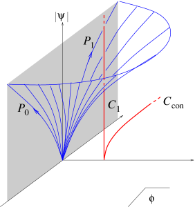
Figure 16: The homotopy ${\mathcal{P}}_{s}$. The shaded region is the orientifold moduli space.

It intersects only with $C_{1}$ of the singular locus at $t=1$ and $s={1\over 2}$. See Figure 16. Thus, we find that ${\mathcal{P}}_{1}$ is homotopic to $-{\mathcal{P}}_{C_{1}}+{\mathcal{P}}_{0}+{\mathcal{P}}_{\infty}$ where ${\mathcal{P}}_{C_{1}}$ is the contour that goes once around the singular locus $C_{1}$ and ${\mathcal{P}}_{\infty}$ is a contour that stays in the large volume limit. See another figure, Fig. 17.

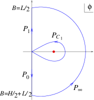
Figure 17: The paths

In [32], the monodromy of the RR-charge for the contour ${\mathcal{P}}_{C_{1}}$ is computed in a basis $\Pi^{\rm G}$ as

$$\Pi^{\rm G}\rightarrow B\Pi^{\rm G};\qquad B=\left(\begin{array}[]{cccccc}1&0&0&0&0&0\\ 0&1&-1&1&-1&1\\ 0&0&2&-1&1&-1\\ 3&-3&4&-3&3&-3\\ -3&3&-4&4&-2&3\\ -3&3&-3&3&-2&3\end{array}\right)$$

We also know that the intersection matrices with respect to the two bases are related as $I^{\rm Cardy}=(1-A)I^{\rm G}(1-A)^{T}$ where

$$A=\left(\begin{array}[]{cccccc}0&1&0&0&0&0\\ 0&0&1&0&0&0\\ 0&0&0&1&0&0\\ 0&0&0&0&1&0\\ 0&0&0&0&0&1\\ -1&0&-1&0&-1&0\end{array}\right)$$

This implies that the two bases are related by

$$\Pi^{\rm Cardy}=U\Pi^{\rm G};\quad U=\pm(1-A)A^{n},$$

for some $n$. In the Cardy basis, the monodromy along the contour $-{\mathcal{P}}_{C_{1}}$ is given by $\Pi^{\rm Cardy}\rightarrow UB^{-1}U^{-1}\Pi^{\rm Cardy}$. Thus, the transformation of the charge basis along the path ${\mathcal{P}}_{1}$ is given by

$$\Pi^{\rm Cardy}=M_{{\mathcal{P}}_{1}}\Pi^{\rm LV};\quad M_{{\mathcal{P}}_{1}}=UB^{-1}U^{-1}M_{{\mathcal{P}}_{0}}.$$ (7.26)

It turns out that $U=(1-A)A^{6}$ is the right choice so that the Cardy branes canceling the tadpole at the Gepner point obey the condition at the large volume with $B=-H+{3\over 2}L$:
$(+++++)$

$${\rm ch}(E)\,{\rm e}^{-B}=32-12H^{2}-4HL.$$ (7.27)

This agrees with the large volume condition.
$(++-++)$ etc

$${\rm ch}(E)\,{\rm e}^{-B}=-8H+{11\over 3}H^{3}$$ (7.28)

This agrees with the large volume condition with $\epsilon[M^{\tau}]=-[M^{\tau}]$.
$(++--+)$ etc

$${\rm ch}(E)\,{\rm e}^{-B}=4H^{2}-4HL$$ (7.29)

This agrees with the large volume condition with $\epsilon[C]=[C]$ and $\epsilon[\ell_{a}]=[\ell_{a}]$.
$(++---)$

$${\rm ch}(E)\,{\rm e}^{-B}=-8H+16L-{1\over 3}H^{3}.$$ (7.30)

The is agrees with the large volume condition with $\epsilon[D]=-[D]$ and $\epsilon[p_{a}]=-[p_{a}]$.

7.3.4 Type of the O-planes

We have determined the orientation $\epsilon[{\bf X}^{\tau}]$ of the O-plane in the two large volume regions, for the $P_{1;\epsilon_{1}...\epsilon_{5}}$-orientifolds. We would now like to know the type of each component of the O-plane. We recall that there are roughly two types of O-planes — O^- and O⁺: $N$ D$p$-brane on top of an O${}^{-}p$-plane support $O(N)$ gauge group while $N$ D$p$-brane on top of an O${}^{+}p$-plane support $Sp(N/2)$. O^--plane has a negative tension and O⁺-plane has a positive tension. Thus, in a supersymmetric configuration where the NSNS tadple is also cancelled, it is impossible to have O-planes of type O⁺ only. In particular, if the O-plane consists of a single component, that must be an O^--plane. Thus, the O9-plane for the $P_{*;+++++}$-orientifold and the O7-plane for the $P_{*;++-++}$-orientifold must be both O^-, as long as there are supersymmetric brane configurations at large volume. For the $P_{1;+-***}$-orientifolds, the O-plane has two (sets of) components which are homologous to each other. At the Gepner point, we found that a configuration without a brane is supersymmetric and tadpole canceling. Thus the two (sets of) O-plane components are of the opposite types, as we have mentioned. In what follows, we discuss the remaining cases, $P_{1;++--+}$ and $P_{1;++---}$.

Let us consider Type II orientifold on a ten-dimensional manifold ${\bf X}$ with respect to an involution $\tau$ of ${\bf X}$. Let

$${\bf X}^{\tau}=\bigcup_{i}W_{i}$$

be the decomposition of the O-plane into connected components. Let $o_{i}=\pm 1$ be the type of the O-plane at $W_{i}$ — it is $\pm 1$ if $W_{i}$ is an O^±-plane. As before we denote the orientation of the O-plane by $\epsilon[W_{i}]$. Then, the D-brane wrapped on $W_{i}$ preserves the same spacetime supersymmetry as this O-plane at $W_{i}$ if its orientation is $o_{i}\epsilon[W_{i}]$. This also tells us the phase of the supersymmetry in the large volume limit. To be specific, we consider the Type IIB orientifolds on a Calabi-Yau three-fold. The overlap of the boundary state for a brane wrapped on $W_{i}$ and the RR-ground state $|0\rangle_{{{}_{\rm RR}}}$ of the lowest R-charge is given by

$${}_{{{}_{\rm RR}}}\langle 0|B_{W_{i}}\rangle = \int_{[W_{i}]}\,{\rm e}^{-i\omega}+\cdots$$

$$= (-i)^{\dim W_{i}}\int_{[W_{i}]}{\omega^{\dim W_{i}}\over\dim W_{i}!}+\cdots$$

where $+\cdots$ are small in the limit $\omega\gg 1$. Note that if $W_{i}$ is a complex submanifold and $[W_{i}]$ is the standard orientation, $\int_{[W_{i}]}\omega^{\dim W_{i}}$ is positive. Thus, in the large volume limit, the phase of the supersymmetry preserved by the O-plane of type $o_{i}$ and orientation $\epsilon[W_{i}]=\epsilon_{i}\cdot[W_{i}]$ is given by

$$\,{\rm e}^{i\theta_{i}}=o_{i}\epsilon_{i}(-i)^{\dim W_{i}}.$$

In particular, in a supersymmetric orientifold, all the components $W_{i}$ must have the same $o_{i}\epsilon_{i}(-i)^{\dim W_{i}}$.

This can be used to find the type of O-plane components (up to an overall sign) for the $P_{1;*****}$-orientifolds. We recall the O-plane orientations for the four relevant cases:

$$\begin{array}[]{l|l|l}&B={H\over 2}+{L\over 2}&B={L\over 2}\\[2.84544pt] \hline\cr P_{1;++--+}&\begin{array}[]{l}\epsilon[C]=-[C]\\ \epsilon[\ell_{a}]=[\ell_{a}]\end{array}&\begin{array}[]{l}\epsilon[C]=-[C]\\ \epsilon[\ell_{a}]=-[\ell_{a}]\end{array}\\[5.69046pt] \hline\cr P_{1;++---}&\begin{array}[]{l}\epsilon[D]=-[D]\\ \epsilon[p_{a}]=[p_{a}]\end{array}&\begin{array}[]{l}\epsilon[D]=[D]\\ \epsilon[p_{a}]=[p_{a}]\end{array}\end{array}$$

Thus, for a common supersymmetry to be conserved, we need that the types must be related as follows

$$\begin{array}[]{l|l|l}&B={H\over 2}+{L\over 2}&B={L\over 2}\\[2.84544pt] \hline\cr P_{1;++--+}&o_{C}=-o_{\ell_{a}}&o_{C}=o_{\ell_{a}}\\[5.69046pt] \hline\cr P_{1;++---}&o_{D}=o_{p_{a}}&o_{D}=-o_{p_{a}}\end{array}$$

To fix the overall sign, we need to look at the tension of the O-plane. Since we need some branes to cancel the tadpole in all cases, we need the total tension to be negative. Let us first discuss the $P_{1;++--+}$ orientifolds. For a Kähler form $\omega=r_{1}H+r_{2}L$, we find

$$\int_{[C]}\omega+\sum_{a=1}^{4}\int_{[\ell_{a}]}\omega=8r_{1}+8r_{2}$$

$$\int_{[C]}\omega-\sum_{a=1}^{4}\int_{[\ell_{a}]}\omega=8r_{1}$$

Thus, the type of the O-plane at $C$ determines the sign of the total tension, and it must always be O^-, $o_{C}=-1$. Next, let us consider the $P_{1;++---}$ orientifolds. In this case, the O-plane at $D$ has clearly larger tension than the ones at $p_{a}$ in the large volume limit. Thus, O-plane at $D$ must always be O^-, $o_{D}=-1$. To summarize, we find that the type of the O-plane components are given by

$$\begin{array}[]{|l|l|l|}\hline\cr&B={H\over 2}+{L\over 2}&B={L\over 2}\\[2.84544pt] \hline\cr P_{1;++--+}&\begin{array}[]{l}C:O^{-}\\ \ell_{a}:O^{+}\end{array}&\begin{array}[]{l}C:O^{-}\\ \ell_{a}:O^{-}\end{array}\\[5.69046pt] \hline\cr P_{1;++---}&\begin{array}[]{l}D:O^{-}\\ p_{a}:O^{-}\end{array}&\begin{array}[]{l}D:O^{-}\\ p_{a}:O^{+}\end{array}\\ \hline\cr\end{array}$$

We found an interesting phenomenon. As we move from one large volume region to another, through the non-geometric region of the constrained Kähler moduli space, the type of O-plane changes: For the $P_{1;++--+}$-orientifold, the O5-plane at the rational curves $\ell_{a}$ change from O$5^{+}$ to O$5^{-}$ while the O5-plane at the genus 9 curve $C$ stays as O$5^{-}$. For the $P_{1;++---}$-orientifold, the O3-planes at $p_{a}$ change from O$3^{-}$ to O$3^{+}$ while the O7-plane at the divisor $D$ remains to be O$7^{-}$. In this discussion, we have assumed that the sign of the total O-plane tension remains the same as the Gepner point. This can be justified by showing that the overlap $\Pi^{\tau\Omega}_{0}$ does not vanish on a path from the Gepner point to the large volume. (However, even if this assumption turns out to be wrong, the change in the type of O-plane we have just discussed remains true.)

This provide a challenge in finding the classification scheme of D-brane charges using K-theory that is valid uniformly in the moduli space. For flat tori, it is known that the D-brane charges in Type II orientifolds are classified by using KR group [75, 76, 77] (see also [78, 79]): For $T^{9-p}/{\mathbb{Z}}_{2}$-orientifold with all O$p^{-}$-planes (resp. all O$p^{+}$-planes), the D-brane charges is classified by KR^-(9-p)-group (resp. KR^-(5-p)-group). One may guess that a similar rule applies when the space is curved. But the above phenomenon tells us that we need something very different to describe the D-brane charges uniformly on the moduli space.

7.4 Comments on Type IIA Orientifolds

Let us consider Type IIA orientifold on a large volume Calabi-Yau manifold $M$ with respect to an antiholomorphic involution $\tau$ of $M$. The O-plane is the fixed point set $M^{\tau}$ which is a special Lagrangian submanifold, and the RR-flux generated by this is determined by the homology class $[M^{\tau}]\in H_{3}(M;{\mathbb{Z}})$. The tadpole cancellation condition $n_{i}$ D6-branes wrapped on special Lagrangian submanifolds $L_{i}$ are given by

$$\sum_{i=1}^{N}n_{i}[L_{i}]=4[M^{\tau}],$$ (7.31)

where $[L_{i}]$ is the homology class of the submanifold $L_{i}$. One obvious solution to this condition is the configuration of four D6-branes wrapped on $M^{\tau}$, but other solutions may exist as well. There can be a spacetime superpotential depending on the $b_{1}(L_{i})$ open string fields as well as the Kähler moduli. There could even be open string fields which are heavy at large volume limit but become light in some interior regions of the Kähler moduli. We would like to compare this with some results obtained at the Gepner point.

Let us first consider the odd $H$ cases. In each of such cases, we found a supersymmetric and tadpole canceling configuration consisting of four copies of one brane $B_{\bf{k-1\over 2},{k-1\over 2}}$. By comparison with the large volume condition, it is natural to identify the brane $B_{\bf{k-1\over 2},{k-1\over 2}}$ as the brane wrapped on the fixed point set $M^{\tau}$. For example, in the case of the quintic, $B_{\bf 1,1}$ is identified as the D6-brane wrapped on the real quintic which has a topology of ${{\mathbb{R}}{\mathbb{P}}}^{3}$. In any of the odd $H$ cases, the open string spectrum at the Gepner point includes massless chiral multiplets charged under $O(4)$ — one or more symmetric tensors and in some cases antisymmetric tensors as well (see Section 4.5.1). Let us consider the quintic case, where there is a single massless matter in the symmetric representation. Can it be consistent with the large volume result? At large volume, there is no open string moduli since the D-brane is wrapped on a simply connected submanifold ${{\mathbb{R}}{\mathbb{P}}}^{3}$. However, as noted in [8], there are choices in specifying the supersymmetric configuration — the choice of the flat gauge connection on the brane. In the present case where the gauge group is $O(4)$, this is given by the $\pi_{1}({{\mathbb{R}}{\mathbb{P}}}^{3})={\mathbb{Z}}_{2}$ holonomy, namely, an element of $O(4)$ which squares to $1$. This is up to gauge transformation, and thus the vacuum manifold is

$${\it V}_{\rm LV}=\Bigl{\{}\,g\in O(4)\,\Bigl{|}\,g^{2}={\bf 1}_{4}\,\Bigl{\}}/{\rm ad}O(4),$$ (7.32)

where $/{\rm ad}O(4)$ is quotient by the action $g\mapsto hgh^{-1}$, $h\in O(4)$. Is there a field theory model consistent with this and the massless spectrum at the Gepner point? This problem is encountered in [8] in the context of a single brane in a theory without orientifold in which there are two vacua at large volume ${\it V}^{\rm single}_{\rm LV}=\{\pm 1\}$: The model is given by the superpotential $W=\phi\psi+\psi^{3}$ where $\phi$ is a closed string field representing the Kähler class and $\psi$ is the open string field. If we identify $\phi=0$ as the Gepner point, $\psi$ is massless at the Gepner point and at large volume there are two vacua $\psi=\pm\sqrt{-\phi/3}$, which is consistent with ${\it V}^{\rm single}_{\rm LV}=\{\pm 1\}$. A natural extension to the current situation is the theory with superpotential

$$W=\phi{\rm Tr}\psi+{\rm Tr}\psi^{3},$$ (7.33)

where $\phi$ is the closed string field representing the Kähler class and and $\psi$ is the symmetric tensor for $O(4)$, $\psi_{ij}=\psi_{ji}$, $i,j=1,2,3,4$. The Gepner point is identified as $\phi=0$ where $\psi$ is massless. Away from that point, say $\phi=-3$, the vacuum equations for $\psi$ are

$$[\psi,\psi^{{\dagger}}]=0,\quad\psi^{2}={\bf 1}_{4},$$

where the first equation is the D-term equation (with $\psi^{T}=\psi$ taken into account) and the second equation is the F-term equation, $\partial_{\psi}W=0$. The vacuum manifold is obtained by moding out the solution space by the adjoint $O(4)$ action. By the D-term equation, $\psi$ can be diagonalized by $U(4)$ matrix and it then follows from $\psi^{T}=\psi$ that $\psi$ is a real matrix. Thus, $\psi$ is a four-by-four real matrix with the constraint $\psi^{T}\psi=\psi^{2}={\bf 1}_{4}$. Namely, the vacuum manifold agrees with one at the large volume (7.32). In this discussion, we have treated the Kähler modulus $\phi$ as a parameter. Of course, in the full string theory, we must treat $\phi$ as a dynamical field and include $\partial_{\phi}W=0$ into the vacuum equations. Then, we obtain an extra constraint ${\rm Tr}\psi=0$ which means that $\psi$ has the same number of $+1$ or $-1$ eigenvalues. It would be interesting to find a similar field theory model for the odd $H$ cases other than the quintic.

Let us next consider an even $H$ case, the two parameter model with $k_{i}=(6,6,2,2,2)$. There is a freedom to dress by quantum symmetry, but we only consider those without dressing for which the large volume region is included in the moduli space. There are six such cases $P^{A}_{+;00000}$, $P^{A}_{+;00001}$, $P^{A}_{+;00011}$, $P^{A}_{+;00111}$ $P^{A}_{+;01000}$. $P^{A}_{+;01001}$. At the Gepner point, only one of them, $P^{A}_{+;01000}$, admits a tadpole canceling supersymmetric solution with exactly four copies of an elementary brane. This brane, $B_{(30111),(30111)}$, is identified in the large volume limit as the O-plane which has topology of $S^{3}$. Since this is simply connected, there is a unique supersymmetric configuration at the large volume. At the Gepner point, we found no massless matter field. A theory consisting of all these is the one with only $O(4)$ super-Yang-Mills without matter and exactly flat Kähler moduli space. In all of the five other cases, we found that there is no consistent supersymmetric configuration with only four branes at the Gepner point (Section 4.6), while “four D6-branes wrapped on the O-plane” is always a solution at large volume. Note that the O-plane has $b_{1}\geq 1$ in these cases, and there are massless open string fields that correspond to moving pairs of D6-branes away from the O-plane, breaking $O(4)$ to $U(2)$ or further to $U(1)^{2}$. One can expect a non-trivial superpotential depending on such open string fields as well as Kähler moduli, and it is conceivable that the supersymmetric vacua with unbroken $O(4)$ misses the Gepner point. It is an interesting problem to verify it by explicit computation of superpotential. Another interesting problem is to analyze the interaction of the supersymmetric solutions we found at the Gepner point and try to connect to the large volume limit.

Appendix

A More General Gepner Models

A Gepner model is defined as the orbifold of the product of minimal models $\prod_{i=1}^{r}M_{k_{i}}$ by the group $\Gamma\simeq{\mathbb{Z}}_{H}$ ($H:={\rm l.c.m}\{k_{i}+2\}$) generated by $\gamma=({\it g},...,{\it g})$ with ${\it g}=\,{\rm e}^{-2\pi iJ_{0}}(-1)^{\widehat{F}}$. It can be used to define a fine compactification to $3+1$ dimensions under the central charge condition

$$c=\sum_{i=1}^{r}{3k_{i}\over k_{i}+2}=9,$$ (A.1)

and the condition on the number of factors

$$r:\,\,\,{\rm odd}.$$ (A.2)

The second condition is needed in order for the RR-charge of the lowest R-charge (corresponding to the holomorphic volume-form of the corresponding Calabi-Yau) to survive the orbifold projection.

Gepner models coming from the linear sigma models of the type described in Section 2.1 always have $r=5$. But there are other models as well. The equation (A.1) has solutions with various number of factors, starting with $r=4$. $r=4$ solutions can be made into $r=5$ by adding a single $k=0$ factor. But there are solutions with $r>5$: According to [38], there are twenty-one models with minimal $r\geq 6$ — fourteen with $r_{\rm min}=6$, four with $r_{\rm min}=7$, two with $r_{\rm min}=8$ and one with $r_{\rm min}=9$. (A solution with even $r$ must be added an odd number of $k=0$ factors so that the condition (A.2) is obeyed.) To be complete we consider these more general cases in this Appendix.

One important identity is

$$\mu:=\sum_{i=1}^{r}\left(1-{1\over k_{i}+2}\right)={r+3\over 2}$$ (A.3)

where we have used the central charge condition (A.1). If we use the second condition (A.2), we find that $\mu$ is an integer. Namely $\sum_{i}{1\over k_{i}+2}$ is an integer. We have implicitly assumed this in the construction of the crosscap states: Look at the the sign factor $(-1)^{\sum_{i}{\nu\over k_{i}+2}}$ in the RR part of the crosscap state (3.16). This does not make sense unless $\sum_{i}{1\over k_{i}+2}$ is an integer.

In the main text of the paper starting Section 3.3 we have assumed that $r=5$. Here we would like to present some formula that is valid for all cases (with odd $r$). The relation between $\,{\rm e}^{\pi iJ_{0}}|\Scr{C}_{P}\rangle$ and $|\Scr{C}_{(-1)^{F}P}\rangle$ changes (for both A and B types) by the sign factor $(-1)^{\mu}$. Thus, the formulae for the total crosscap states are modified as

$$(\ref{CARtotal})\longrightarrow |C_{\omega;{\bf m}}\rangle_{{{}_{\rm RR}}}=|\Scr{C}_{P^{A}_{\omega;{\bf m}}}\rangle\otimes|\Scr{C}_{+}^{\rm\,st}\rangle_{{{}_{\rm RR}}}-(-1)^{\mu}\omega|\Scr{C}_{(-1)^{F}P^{A}_{\omega;{\bf m}}}\rangle\otimes|\Scr{C}_{-}^{\rm\,st}\rangle_{{{}_{\rm RR}}},$$

$$(\ref{CBRtotal})\longrightarrow |C^{B}_{\omega;{\bf m}}\rangle_{{{}_{\rm RR}}}=|\Scr{C}_{P^{B}_{\omega;{\bf m}}}\rangle\otimes|\Scr{C}_{+}^{\rm\,st}\rangle_{{{}_{\rm RR}}}-(-1)^{\mu}\widetilde{\omega}^{-1}|\Scr{C}_{(-1)^{F}P^{B}_{\omega;{\bf m}}}\rangle\otimes|\Scr{C}_{-}^{\rm\,st}\rangle_{{{}_{\rm RR}}},$$

If $\mu$ is even (note that $\mu=4$ (even) if $r=5$), there is no difference in the discussion after Section 3.3. But there is some change if $\mu$ is odd. The largest effect is in the action of parities on the branes. The transformation rules (4.24)-(4.27) and (6.14)-(6.15) changes by sign (orientation). As a consequence, this affects the set of parity invariant D-branes. The analysis of the structure of Chan-Paton factor goes through as in the discussion of $r=5$, with an obvious modification of the result.

Addition of two $k=0$ factors shifts even $\mu$ to odd $\mu$ and vice versa. What we have seen is that this has a non-trivial effect on the physics involving branes in the orientifold model. In fact, without orientifold, addition of even number of $k=0$ factors makes no difference since the orbifold action is trivial on such pair of $k=0$ factors. This is also true for the case involving D-branes (before orientifold): for A-branes, the orbifold group flips the orientation of the brane in a $W=X^{2}$ factor but a pair of such flips cancel against each other. For B-branes the same can be said (this is known as the Knörrer periodicity [80]). However, with an orientifold, this step 2 periodicity is doubled to step 4. This reminds us of the Bott periodicity: complex K-theory has periodicity 2 but Real K-theory has periodicity 8.

B Some Detail

We explain the projection factors (4.25) and (4.26) that are used to read the parity action on short-orbit branes.

We first compute the ${\mathbb{Z}}_{2}$ projection factor for the open string stretched from a short-orbit brane $\widehat{B}^{(\varepsilon)}_{\bf\bar{L},\bar{M}}$ to another $\widehat{B}^{(\varepsilon^{\prime})}_{\bf L,M}$. To this end, let us consider the loop-channel expansion of the relevant overlaps in the minimal model with even $k$,

$$\langle\Scr{B}_{\frac{k}{2},\bar{M},\bar{S}}|q_{t}^{H}|\Scr{B}_{\frac{k}{2},M,S}\rangle_{{{}_{\rm NSNS}}\atop{{}_{\rm RR}}}=\sum_{l\atop s=0,1}N_{\frac{k}{2}\frac{k}{2}}^{l}(\pm 1)^{s}\chi_{l,\bar{M}-M,\bar{S}-S+2s}(\tau_{l}),$$

$$\langle\Scr{B}_{\frac{k}{2},\bar{M},\bar{S}}|q_{t}^{H}|\Scr{B}_{\frac{k}{2},M,S}\rangle_{(\mp 1)^{F}a^{k+2}}=\sum_{l\atop s=0,1}N_{\frac{k}{2}\frac{k}{2}}^{l}(\pm 1)^{s}(-1)^{\frac{1}{2}(l+\bar{M}-M-\bar{S}^{2}+S^{2})}\chi_{l,\bar{M}-M,\bar{S}-S+2s}(\tau_{l})$$

This is enough to see the open string states labeled by $\otimes_{i=1}^{r}(l_{i},n_{i},s_{i})$ are subject to the projection

$$\frac{1}{2}\left(1+\gamma^{H/2}\right)~{}=~{}\frac{1}{2}\left(1+\varepsilon\varepsilon^{\prime}\prod_{w_{i}\,{\rm odd}}(-1)^{\frac{1}{2}(l_{i}+n_{i}-s)}\right),$$ (B.2)

where $s=0$ for NS states and $1$ for R ones. This is nothing but (4.25).

Let us next find the projection factor that appears in the parity twisted partition function. To do this, let us consider the minimal model with even $k$, and take the Möbius strip amplitude

$${}_{{{}_{\rm NSNS}}}\langle\Scr{B}_{\frac{k}{2},M,S}|q_{t}^{H}|\Scr{C}^{A}_{(\pm 1)^{F}g^{m}\widetilde{P}_{A}}\rangle$$ (B.3)

$$= \sum_{l}\delta^{(2)}_{l}(-1)^{m+\frac{l}{2}}\left\{e^{\mp\frac{\pi i}{4}}\hat{\chi}_{l,2M-2m,2S}-e^{\pm\frac{\pi i}{4}}\hat{\chi}_{l,2M-2m,2S+2}\right\}(\tau)$$

where

$$\hat{\chi}_{l,n,s}(\tau)=e^{-\pi i(\frac{l(l+2)-n^{2}}{4k+8}+\frac{s^{2}}{8}-\frac{c}{24})}\chi_{l,n,s}(\tau+1/2).$$ (B.4)

Let us see how it changes under the shift $m\rightarrow m+\frac{k+2}{2}$. This tell us that the open string state $(l,n,s)$ on the Möbius strip (B.3) has the following eigenvalue of $g^{\frac{k+2}{2}}$:

$$g^{\frac{k+2}{2}}=\pm i(-1)^{\frac{l+n}{2}+S}.$$ (B.5)

One can also perform a similar analysis on the RR sector states. Let us then take a short orbit A-brane $\widehat{B}^{\pm,A}_{{\bf L,M}}$ and an A-parity $P^{A}_{\omega,{\bf m}}$. Using (B.5) for each minimal model, we can now easily find the eigenvalue of $\gamma^{H/2}$ for the open string state $\otimes_{i=1}^{r}(l_{i},n_{i},s_{i})$ on the Möbius strip. The result is independent of the choice of branes and reads

$$\gamma^{H/2}=\omega^{\frac{H}{2}}(-1)^{\frac{\sigma}{2}}\prod_{w_{i}~{}{\rm odd}}(-1)^{\frac{1}{2}(l_{i}+n_{i}-s)},$$ (B.6)

where $s=0$ for NS states and $1$ for R ones as before, and $\sigma$ is the number of $i$’s such that $w_{i}$ is odd. This leads to the projection factor (4.26).

C Integral bases of three-cycles in the quintic

In the main text, we have seen that the most convenient way to write down and solve the tadpole conditions is to find an integral basis of the charge lattice, so that the coefficients in the equations (4.40) are manifestly integer. In this appendix, we describe how such a basis can be found for A-type branes on the quintic. We will also describe an alternative way of solving the tadpole conditions using $g_{i}$ polynomials.

Integral basis

In a single minimal model with $k=3$, the charges of A-type branes span a 4-dimensional lattice which is generated by the $5$ branes $\Scr{B}^{A}_{0,M,1}$ with $M=1,3,5,7,9$. As is easiest to see in the Landau-Ginzburg picture, these $5$ charges satisfy one linear relation: Their sum is zero. We can fit the set $\Lambda$ of five charges modulo this one relation into an exact sequence

$$0\longrightarrow\{R\}\longrightarrow{\mathbb{A}}_{5}\longrightarrow\Lambda\longrightarrow 0$$ (C.1)

where ${\mathbb{A}}_{5}$ stands for the set $\{n=0,1,2,3,4\}$ representing the charges $Q_{n}$ of the brane $\Scr{B}^{A}_{0,2n+1,1}$, and $R$ is the relation

$$R\mapsto\sum_{n}Q_{n}$$

There is an obvious ${\mathbb{Z}}_{5}$ action on ${\mathbb{A}}_{5}$ and on (C.1) which cyclically permutes the five elements, and leaves $R$ invariant.

If we now take the tensor product of $5$ such minimal models, the charge lattice has dimension $4^{5}=1024$. It is generated by the tensor products $Q({\bf n})=\prod_{i}Q_{n_{i}}$ modulo the relations

$$R_{1}(i;{\bf n})=\sum_{n_{i}}Q(n_{1},\ldots,n_{5})$$

where ${\bf n}=(n_{1},\ldots,\widehat{n_{i}},\ldots n_{5})$. Thus we have $5^{5}$ charges with $5^{5}$ relations, but these relations are not all independent. Namely, we have the relations between relations

$$R_{2}(i,j;{\bf n})=\sum_{n_{i}}R_{1}(j;({\bf n},n_{i}))-\sum_{n_{j}}R_{1}(i;({\bf n},n_{j}))$$

where now ${\bf n}=(n_{1},\ldots,\widehat{n_{i}},\ldots,\widehat{n_{j}},\ldots,n_{5})$. Continuing this way, we obtain the long-exact sequence for the set of charges $\Lambda^{\rm ten}$ of the tensor product

$$0\longrightarrow\{R_{5}\}\longrightarrow 5{\mathbb{A}}_{5}\longrightarrow 10({\mathbb{A}}_{5})^{2}\longrightarrow 10({\mathbb{A}}_{5})^{3}\longrightarrow 5({\mathbb{A}}_{5})^{4}\longrightarrow({\mathbb{A}}_{5})^{5}\longrightarrow\Lambda^{\rm ten}\longrightarrow 0$$ (C.2)

from which we see that the dimension of the charge lattice is indeed $4^{5}$. The advantage of this representation is that it is now trivial to take the ${\mathbb{Z}}_{5}$ orbifold. All relations $R_{s}$ with $s<5$ are related to one another under the diagonal ${\mathbb{Z}}_{5}$ action, while $R_{5}$ is invariant. Thus, the untwisted charges can be represented by the sequence

$$0\longrightarrow\{R_{5}\}\longrightarrow 5({\mathbb{A}}_{5})^{0}\longrightarrow 10{\mathbb{A}}_{5}\longrightarrow 10({\mathbb{A}}_{5})^{2}\longrightarrow 5({\mathbb{A}}_{5})^{3}\longrightarrow({\mathbb{A}}_{5})^{4}\longrightarrow\Lambda^{\rm Gep}\longrightarrow 0$$ (C.3)

from which we read off the dimensions of the charge lattice of the Gepner model to be $204$, as expected. To obtain a basis of $\Lambda^{\rm Gep}$, we take a section of (C.3). In view of solving the tadpole conditions, it is most useful to do this in such a way that respects the action of the parity. The parity acts in a single minimal model on $Q_{n}$ as $0\mapsto 4$, $1\mapsto 3$, and $2\mapsto 2$, and similarly on all the relations. We will show how this language simplifies finding the explicit form of (4.40) in appendix D.

Solving the tadpole conditions with $g_{i}$ polynomials

The tadpole cancellation condition can also be written in a simple form by using the $g_{i}$-polynomials. Here we again restrict our attention to the RR-charges and tadpoles sitting in the untwisted sector. Let us introduce the $(k_{i}+2)$-dimensional shift matrices $g_{i}$ satisfying $g_{i}^{k_{i}+2}=1$, and associate the following polynomial to each D-brane

$$Q_{\bf L,M}(g_{i})=\prod_{i=1}^{5}\left(\sum_{n_{i}=0}^{L_{i}}g_{i}^{n_{i}+(M_{i}-L_{i})/2}\right),$$ (C.4)

representing its RR-charge. Let us also associate similar $g_{i}$-polynomials to the orientifolds by first expressing their RR-charges in terms of D-branes and then using the above formula. These polynomials of $g_{i}$ are useful in computing the (twisted) Witten indices between D-branes and O-planes. The index between the branes $B$ and $B^{\prime}$ is given by the diagonal element(more precisely, the product of diagonal elements) of the matrix

$$I=Q_{B}(g_{i})Q_{B^{\prime}}(g_{i}^{-1})\prod_{i=1}^{5}(1-g_{i}^{-1})\sum_{\nu=1}^{H}(g_{1}g_{2}g_{3}g_{4}g_{5})^{\nu}$$ (C.5)

Since the last factor in the right hand side is the projection onto the states on which $g_{5}^{-1}=g_{1}g_{2}g_{3}g_{4}$, we can eliminate $g_{5}$ and obtain

$$I = Q_{B}(g_{i})Q_{B^{\prime}}(g_{i}^{-1})(1-g_{1}^{-1})(1-g_{2}^{-1})(1-g_{3}^{-1})(1-g_{4}^{-1})(1-g_{1}g_{2}g_{3}g_{4})$$ (C.6)

$$\times\sum_{\nu=1}^{w_{5}}(g_{1}g_{2}g_{3}g_{4})^{\nu(k_{5}+2)},$$

where the index is read off as the diagonal elements. This agrees with the formula for quintic given in [8]. The RR-charges of any configurations of branes and the O-plane are therefore expressed as polynomials of $g_{i}$,

$$(\mbox{RR-charge})=\sum_{m_{i}=0}^{k_{i}+1}N_{m_{1}m_{2}m_{3}m_{4}m_{5}}g_{1}^{m_{1}}g_{2}^{m_{2}}g_{3}^{m_{3}}g_{4}^{m_{4}}g_{5}^{m_{5}}.$$ (C.7)

The configuration is free of tadpoles when the sum of $g_{i}$-polynomials of the constituent D-branes and the O-plane vanishes up to

$$1+g_{i}+\cdots+g_{i}^{k_{i}+1}=0,~{}~{}~{}g_{1}g_{2}g_{3}g_{4}g_{5}=1.$$ (C.8)

It is cumbersome to have these equivalence relations in analyzing the polynomial. Therefore, it is more convenient to use the relations (C.8) to bring the polynomial into the following gauge

$$\sum_{m_{a}=0}^{k_{a}+1}N_{m_{1}\cdots m_{a}\cdots m_{5}}=0,~{}~{}~{}N_{m_{1}m_{2}m_{3}m_{4}m_{5}}=N_{m_{1}+1,m_{2}+1,m_{3}+1,m_{4}+1,m_{5}+1}$$ (C.9)

and see whether each coefficient is vanishing or not. This is certainly possible because each of the polynomials $Q_{\bf L,M}(g_{i})$ can be brought to this gauge (C.9) in the following way.

$$Q_{\bf L,M}(g_{i}) = \frac{1}{H}\sum_{\nu=0}^{H-1}\sum_{n_{i}=0}^{k_{i}+1}\prod_{i=1}^{5}(f_{L_{i},n_{i}}g_{i}^{n_{i}+\nu+(M_{i}-L_{i})/2)}),$$

$$f_{L_{i},n_{i}} = \left\{\begin{array}[]{ll}1-{\textstyle\frac{L_{i}+1}{k_{i}+2}}&(0\leq n_{i}\leq L_{i})\\ -{\textstyle\frac{L_{i}+1}{k_{i}+2}}&({\rm otherwise})\end{array}\right.$$ (C.12)

As was noted before, these $g_{i}$-polynomials can only express the RR-charges corresponding to polynomial deformations of hypersurfaces defining the target space. In the two parameter model with $(k_{i}+2)=(8,8,4,4,4)$ there are six missing RR charges sitting in the twisted sector. One can develop a similar argument using polynomials for those RR-charges, too.

We can again see that the number of independent components of $N_{m_{1}m_{2}m_{3}m_{4}m_{5}}$ agrees with the number of RR ground states in the untwisted sector, which take the form (4.41),

$$|l_{i}\rangle=\prod_{i=1}^{5}|l_{i},l_{i}+1,1\rangle\times|l_{i},-l_{i}-1,-1\rangle~{}~{}~{}(1\leq l_{i}+1\leq k_{i}+1,~{}\sum_{i}{\textstyle\frac{l_{i}+1}{k_{i}+2}}\in{\mathbb{Z}})$$ (C.13)

To see this, let us take the Fourier transform of $N_{m_{1}m_{2}m_{3}m_{4}m_{5}}$:

$$\widetilde{N}_{n_{1}n_{2}n_{3}n_{4}n_{5}}=\sum_{m_{i}\in{\mathbb{Z}}_{k_{i}+2}}\exp(\sum_{i}\frac{2\pi im_{i}n_{i}}{k_{i}+2})N_{m_{1}m_{2}m_{3}m_{4}m_{5}}$$ (C.14)

Then $\widetilde{N}_{n_{1}n_{2}n_{3}n_{4}n_{5}}$ are nonzero only when $n_{i}$ are all nonzero mod $k_{i}+2$ and $\sum_{i}\frac{n_{i}}{k_{i}+2}\in{\mathbb{Z}}$, which is the same condition as the RR ground states satisfy under the identification $n_{i}\leftrightarrow l_{i}+1$ (mod $k_{i}+2$). So $\widetilde{N}_{n_{1}n_{2}n_{3}n_{4}n_{5}}$ has as many independent components as there are untwisted RR vacua.

Of all the linear equations, there are some equations among the tadpole cancellation conditions in which all the D-branes appear with positive definite coefficients. These essentially come from the overlaps with the RR ground states $|\nu\rangle$, namely, those with $l_{i}=\nu$ mod $k_{i}+2$ for all $i$. The reason for the positivity is that the overlaps of D-branes or O-planes with any of these states have the same phases if they preserve the same spacetime supersymmetry. These equations are particularly important, because they ensure that there are only finite number of tadpole canceling configurations. These equations also contain the condition that the sum of D-brane tensions must cancel the O-plane tension. One can obtain these special equations from $g_{i}$-polynomials by setting $g_{i}=g^{w_{i}}$, where $g$ is a $H$-dimensional shift matrix.

D Tadpole conditions for ${\mathbb{Z}}_{5}$ orbifold of quintic

In this appendix, we discuss the tadpole conditions for Type IIB orientifolds of the orbifold of the quintic by the ${\mathbb{Z}}_{5}$ symmetry called $[1,4,0,0,00]$ in the notation of [25]. By mirror symmetry, this is equivalent to Type IIA orientifold of $({\mathbb{Z}}_{5})^{2}$ orbifold of the quintic. In B-type language, the model has $2h^{1,1}+2=12$ RR charges to cancel (the fact that $h^{2,1}=49$ will not be important). The analogs of RS branes in such orbifolds have been discussed for instance in [81], and are also straightforward to obtain in the Landau-Ginzburg picture. It is easy to see that the branes are labeled as $\Scr{B}_{{\bf L},{\bf M},S}$ with ${\bf L}$ as before and ${\bf M}=(M_{1},M_{2},M_{3},M_{4},M_{5})$ modulo a $({\mathbb{Z}}_{5})^{3}$ identification.

We can present an integral basis of the charge lattice similarly to (C.3) via

$$0\longrightarrow{R_{3}}\longrightarrow 3({\mathbb{A}}_{5})^{0}\longrightarrow 3{\mathbb{A}}_{5}\longrightarrow({\mathbb{A}}_{5})^{2}\longrightarrow\Lambda^{\rm orbi}\longrightarrow 0$$ (D.1)

such that $\Lambda^{\rm orbi}$ indeed has dimension $25-15+3-1=12$. We now take a section through (D.1) and specify an integral basis as the charges of the branes with ${\bf L}={\bf 0}$ and ${\bf M}=2{\bf n}+1$ with

$$\begin{array}[]{l}{\bf n}\in\Bigl{\{}[0,0,2,2,2],[0,4,2,2,2],[1,0,2,2,2],[1,1,2,2,2],[1,3,2,2,2],[1,4,2,2,2],\\ \qquad[4,4,2,2,2],[4,0,2,2,2],[3,4,2,2,2],[3,3,2,2,2],[3,1,2,2,2],[3,0,2,2,2]\Bigr{\}}\end{array}$$

where $[\cdots]$ denotes $({\mathbb{Z}}_{5})^{3}$ orbits and where the second line is obviously the parity image of the first.

As before, branes preserving the same supersymmetry as the O-plane have arbitrary ${\bf L}$ and $\sum M_{i}=0\bmod 5$ and appropriate $S$ label depending on the parity of $\sum L_{i}$. Obviously, the charge of such branes does not depend on the permutations of $L_{3},L_{4},L_{5}$, so we have the following representatives of ${\bf L}$ labels

$$\begin{array}[]{ll}{\bf L}=&(0,0,0,0,0),\\ &(1,0,0,0,0),(0,1,0,0,0),(0,0,1,0,0),\\ &(1,1,0,0,0),(1,0,1,0,0),(0,1,1,0,0),(0,0,1,1,0),\\ &(1,1,1,0,0),(1,0,1,1,0),(0,1,1,1,0),(0,0,1,1,1),\\ &(1,1,1,1,0),(1,0,1,1,1),(0,1,1,1,1)\\ &(1,1,1,1,1)\end{array}$$ (D.2)

where we have ordered the branes according to increasing tension. The possible ${\bf M}$ labels are ($\bmod 5$ and modulo $({\mathbb{Z}}_{5})^{3}$):

$${\bf M}=[0,0,0,0,0],[1,4,0,0,0],[4,1,0,0,0],[2,3,0,0,0],[3,2,0,0,0]$$ (D.3)

The first of these is obviously invariant under the parity, while the others are each others image. Thus, we have a total of $16\times 3=48$ different charges to consider in the tadpole cancellation. We will denote by $n_{1},\ldots n_{48}$ the number of times a given charge appears.

By utilizing the well-known expressions for the charges of branes in the minimal model (see (C.4) or (6.24)), we can compute the RR charges of all branes on the list in the basis described above. This leads to the following $6$ equations on the $48$ $n_{i}$’s

$$(n_{1},\ldots,n_{48})\left(\hbox{\scriptsize$\begin{array}[]{cccccc}2&2&0&0&0&0\\ 2&2&1&0&0&0\\ 1&1&1&-1&0&0\\ 2&0&0&1&0&-1\\ 2&0&0&1&-1&1\\ 1&0&1&0&1&0\\ 2&0&0&1&0&1\\ 2&0&1&1&1&-1\\ 1&0&0&0&-1&0\\ 2&0&-1&2&0&0\\ 2&0&1&0&0&0\\ 1&0&1&0&0&0\\ 4&2&2&0&0&0\\ 4&2&1&0&0&0\\ 2&1&0&1&0&0\\ 4&2&0&1&-1&-1\\ 4&2&2&0&1&0\\ 2&1&1&0&0&1\\ 4&2&1&1&1&1\\ 4&2&1&0&-1&0\\ 2&1&1&0&0&-1\\ 4&2&-1&2&0&0\\ 4&2&2&0&0&0\\ 2&1&2&-1&0&0\\ 6&2&3&0&0&0\\ 6&2&1&2&0&0\\ 3&1&0&1&0&0\\ 6&2&0&2&-1&-2\\ 6&2&2&1&0&1\\ 3&1&2&0&1&1\\ 6&2&1&2&1&2\\ 6&2&2&1&0&-1\\ 3&1&1&0&-1&-1\\ 6&2&-2&4&0&0\\ 6&2&3&0&0&0\\ 3&1&3&-1&0&0\\ 10&4&5&0&0&0\\ 10&4&2&2&0&0\\ 5&2&0&2&0&0\\ 10&4&0&3&-2&-3\\ 10&4&4&1&1&1\\ 5&2&3&0&1&2\\ 10&4&2&3&2&3\\ 10&4&3&1&-1&-1\\ 5&2&2&0&-1&-2\\ 16&6&8&0&0&0\\ 16&6&3&4&0&0\\ 8&3&0&3&0&0\end{array}$}\right)=(32,12,0,12,0,0)$$ (D.4)

Inspection reveals that the first two of these equations are nothing but the equations (6.32) that we have solved in the context of B-type orientifold of quintic. To see this, one has to take into account that for branes not invariant under parity, $n_{i}$ denotes the number of times the brane and its image under parity appear, and the fact that the mass depends only on the number of $1$’s in the ${\bf L}$ label. Thus, to find solutions of (D.4), we can take some solution of (6.32) and scan through all ways of distributing this mass among the branes on the list of $48$ with the same tension.

Here are a few examples of tadpole canceling brane configurations for the ${\mathbb{Z}}_{5}$ orbifold of the quintic obtained in this way.
Example 1

$$(B_{(00111),(20111)}+\mbox{\footnotesize image})+(\overline{B_{(11110),(39116)}}+\mbox{\footnotesize image})+2B_{(11111),(11111)}$$

Example 2

$$4(\overline{B_{(00000),(20666)}}+\mbox{\footnotesize image})+2(B_{(00100),(20166)}+\mbox{\footnotesize image})+B_{(00100),(66166)}$$

$$+(B_{(01110),(25116)}+\mbox{\footnotesize image})+(B_{(10000),(34666)}+\mbox{\footnotesize image})+3(B_{(10000),(70666)}+\mbox{\footnotesize image})$$

$$+\overline{B_{(11110),(11116)}}$$

Example 3

$$3(\overline{B_{(00000),(20666)}}+\mbox{\footnotesize image})+\overline{B_{(00000),(66666)}}+(\overline{B_{(00000),(84666)}}+\mbox{\footnotesize image})$$

$$+5(B_{(00100),(20166)}+\mbox{\footnotesize image})+B_{(00100),(66166)}+2B_{(01000),(61666)}+2B_{(10000),(16666)}$$

$$+B_{(11111),(11111)}$$

Particle spectrum

The spectrum of massless matters for these brane configurations is analyzed in a similar way as in the case of ordinary quintic. Here we only present the results.

${}^{\rm gauge}_{\rm group}$	$\sharp$	${\bf L},~{}{\bf M},~{}S$	1	2	3	4	5
$U(1)$	1	(00111),(20111),0	12	0	0	3	0
	2	(00111),(02111),0	0	12	3	0	0
$U(1)$	3	(11110),(39116),2	0	3	12	7+3	10
	4	(11110),(93116),2	3	0	7+3	12	10
$O(2)$	5	(11111),(11111),0	0	0	10	10	13+12

Example 1

The first example consists of five kinds of branes, $B_{1}+B_{2}+B_{3}+B_{4}+2B_{5}$, where $B_{5}$ is parity invariant and $B_{2},B_{4}$ are parity images of $B_{1},B_{3}$. The spectrum of chiral matters is summarized in the table above.

The gauge group is $U(1)^{2}\times O(2)$, and the labels $({\bf L,M},S)$ of five D-branes are presented in the second column. The $5\times 5$ numbers give the multiplicities of chiral primary states on $i\!-\!j$ string ($i,j=1,\cdots,5$). $3\!-\!4,4\!-\!3$ and $5\!-\!5$ strings are parity invariant, and they belong to symmetric or antisymmetric tensor representations of gauge group according to their parity eigenvalues. The numbers $7+3$ or $13+12$ represent the multiplicities of symmetric and antisymmetric representations.

The table contains nine blocks. Upper off-diagonal blocks are related with lower off-diagonal ones by parity, namely, the multiplicity of matters on $i\!-\!j$ string is the same as that of $P(j)\!-\!P(i)$ string. As was explained in section 5, the spectrum is chiral if there is a block with the following property

• An off-diagonal block corresponding to one unitary and one non-unitary groups, with numbers

  $$\left(\begin{array}[]{c}a\\ b\end{array}\right)~{}~{}{\rm or}~{}~{}(a~{}b),~{}~{}~{}a\neq b$$

• An off-diagonal block corresponding to two different unitary groups, with numbers

  $$\left(\begin{array}[]{cc}a&b\\ c&d\end{array}\right),~{}~{}~{}a\neq d~{}~{}{\rm or}~{}~{}b\neq c.$$

• A diagonal block for a unitary group, with numbers

  $$\left(\begin{array}[]{cc}a&b_{s}+b_{a}\\ c_{s}+c_{a}&a\end{array}\right),~{}~{}~{}b_{s}\neq c_{s}~{}~{}{\rm or}~{}~{}b_{a}\neq c_{a}$$

The table shows that the first example is non-chiral.

The other two examples are chiral, as can be seen from the tables below. Note that there are no antisymmetric tensor representations of $U(1)$ or $O(1)$.

${}^{\rm gauge}_{\rm group}$	$\sharp$	${\bf L},~{}{\bf M},~{}S$	1	2	3	4	5	6	7	8	9	10	11	12
$U(4)$	1	(00000),(20666),2	0	0	2	0	1	0	1	0	0	0	1	0
	2	(00000),(02666),2	0	0	0	2	1	0	0	1	3	0	0	0
$U(2)$	3	(00100),(20166),0	2	0	2	0	1	0	3	1	2	0	0	0
	4	(00100),(02166),0	0	2	0	2	1	0	0	0	0	2	0	0
$O(1)$	5	(00100),(66166),0	1	1	1	1	2	2	1	2	0	1	0	3
$U(1)$	6	(01110),(25116),0	0	1	0	3	1	5	1	0	1	2	1	5
	7	(01110),(07116),0	0	0	0	0	2	1	5	1	0	1	2	2
$U(1)$	8	(10000),(34666),0	3	0	0	2	0	0	1	0	0	3	0	2
	9	(10000),(98666),0	1	0	0	1	2	1	0	3	0	1	0	1
$U(3)$	10	(10000),(70666),0	0	1	0	0	0	2	1	0	0	0	1	0
	11	(10000),(52666),0	0	0	2	0	1	1	2	1	3	0	0	2
$O(1)$	12	(11110),(11116),2	0	0	0	0	3	2	5	1	2	2	0	6

Example 2
${}^{\rm gauge}_{\rm group}$ $\sharp$ ${\bf L},~{}{\bf M},~{}S$ 1 2 3 4 5 6 7 8 9 10 11 $U(3)$ 1 (00000),(20666),2 0 0 0 0 0 2 0 1 0 3 0 2 (00000),(02666),2 0 0 0 0 0 0 2 1 3 0 0 $O(1)$ 3 (00000),(66666),2 0 0 0 0 0 1 1 2 0 0 1 $U(1)$ 4 (00000),(84666),2 0 0 0 0 0 1 0 0 0 1 0 5 (00000),(48666),2 0 0 0 0 0 0 1 0 1 0 0 $U(5)$ 6 (00100),(20166),0 2 0 1 1 0 2 0 1 1 0 0 7 (00100),(02166),0 0 2 1 0 1 0 2 1 0 1 0 $O(1)$ 8 (00100),(66166),0 1 1 2 0 0 1 1 2 0 0 3 $O(2)$ 9 (01000),(61666),0 3 0 0 1 0 0 1 0 0 3 1 $O(2)$ 10 (10000),(16666),0 0 3 0 0 1 1 0 0 3 0 1 $O(1)$ 11 (11111),(11111),0 0 0 1 0 0 0 0 3 1 1 13 Example 3

References

- [1]
-
[2]
M. Douglas, “Mastering N=1”, talk at Strings 2002, Cambridge,
July 17, 2002;
http://www.damtp.cam.ac.uk/strings02/avt/douglas/ - [3] S. B. Giddings, S. Kachru and J. Polchinski, “Hierarchies from fluxes in string compactifications,” Phys. Rev. D 66 (2002) 106006 [hep-th/0105097].
- [4] S. Kachru, R. Kallosh, A. Linde and S. P. Trivedi, “De Sitter vacua in string theory,” Phys. Rev. D 68 (2003) 046005 [hep-th/0301240].
- [5] D. Gepner, “Space-Time supersymmetry in compactified string theory and superconformal models,” Nucl. Phys. B 296 (1988) 757; “Exactly solvable string compactifications on manifolds of holonomy,” Phys. Lett. B 199 (1987) 380.
- [6] J. L. Cardy, “Boundary Conditions, Fusion Rules And The Verlinde Formula,” Nucl. Phys. B 324, 581 (1989).
- [7] A. Recknagel and V. Schomerus, “D-branes in Gepner models,” Nucl. Phys. B 531 (1998) 185 [hep-th/9712186].
- [8] I. Brunner, M. R. Douglas, A. E. Lawrence and C. Romelsberger, “D-branes on the quintic,” JHEP 0008 (2000) 015 [hep-th/9906200].
- [9] G. Pradisi, A. Sagnotti and Y. S. Stanev, “Planar duality in SU(2) WZW models”, Phys. Lett. B 354 (1995) 279 [hep-th/9503207]; “The Open descendants of nondiagonal SU(2) WZW models,” Phys. Lett. B 356, (1995) 230 [hep-th/9506014]; “Completeness Conditions for Boundary Operators in 2D Conformal Field Theory,” Phys. Lett. B 381, (1996) 97 [hep-th/9603097].
- [10] P. Bantay, “The Frobenius-Schur indicator in conformal field theory”, Phys. Lett. B 394, (1997) 89 [hep-th/9610192].
- [11] L. R. Huiszoon, A. N. Schellekens and N. Sousa, “Klein bottles and simple currents,” Phys. Lett. B 470 (1999) 95 [hep-th/9909114].
- [12] J. Fuchs, L. R. Huiszoon, A. N. Schellekens, C. Schweigert and J. Walcher, “Boundaries, crosscaps and simple currents,” Phys. Lett. B 495 (2000) 427 [hep-th/0007174].
- [13] C. Angelantonj and A. Sagnotti, “Open strings,” Phys. Rept. 371, 1 (2002) [hep-th/0204089].
- [14] J. Fuchs and C. Schweigert, “Symmetry breaking boundaries. I: General theory,” Nucl. Phys. B 558, 419 (1999) [hep-th/9902132].
- [15] I. Brunner and K. Hori, “Notes on orientifolds of rational conformal field theories,” [hep-th/0208141].
- [16] R. Blumenhagen and A. Wisskirchen, “Spectra of 4D, N = 1 type I string vacua on non-toroidal CY threefolds”, Phys. Lett. B 438 (1998) 52 [hep-th/9806131].
- [17] C. Angelantonj, M. Bianchi, G. Pradisi, A. Sagnotti and Y. S. Stanev, “Comments on Gepner models and type I vacua in string theory”, Phys. Lett. B 387 (1996) 743 [hep-th/9607229].
- [18] I. Brunner and K. Hori, “Orientifolds and mirror symmetry,” hep-th/0303135.
- [19] S. Govindarajan and J. Majumder, “Orientifolds of type IIA strings on Calabi-Yau manifolds,” hep-th/0305108; “Crosscaps in Gepner models and type IIA orientifolds,” hep-th/0306257.
- [20] L. R. Huiszoon and K. Schalm, “BPS orientifold planes from crosscap states in Calabi-Yau compactifications,” JHEP 0311 (2003) 019 [hep-th/0306091].
- [21] J. Fuchs and C. Schweigert, “Branes: From free fields to general backgrounds,” Nucl. Phys. B 530, 99 (1998) [hep-th/9712257].
- [22] I. Brunner and V. Schomerus, “D-branes at singular curves of Calabi-Yau compactifications,” JHEP 0004, 020 (2000) [hep-th/0001132].
- [23] J. Fuchs, C. Schweigert and J. Walcher, “Projections in string theory and boundary states for Gepner models,” Nucl. Phys. B 588, 110 (2000) [hep-th/0003298].
- [24] J. Fuchs, P. Kaste, W. Lerche, C. A. Lutken, C. Schweigert and J. Walcher, “Boundary fixed points, enhanced gauge symmetry and singular bundles on K3,” Nucl. Phys. B 598, 57 (2001) [hep-th/0007145].
- [25] B. R. Greene and M. R. Plesser, “Duality In Calabi-Yau Moduli Space,” Nucl. Phys. B 338 (1990) 15.
- [26] J. M. Maldacena, G. W. Moore and N. Seiberg, “Geometrical interpretation of D-branes in gauged WZW models,” JHEP 0107 (2001) 046 [hep-th/0105038].
- [27] D. E. Diaconescu and M. R. Douglas, “D-branes on stringy Calabi-Yau manifolds,” hep-th/0006224.
- [28] D. E. Diaconescu and C. Romelsberger, “D-branes and bundles on elliptic fibrations,” Nucl. Phys. B 574, 245 (2000) [hep-th/9910172].
- [29] P. Kaste, W. Lerche, C. A. Lutken and J. Walcher, “D-branes on K3-fibrations,” Nucl. Phys. B 582, 203 (2000) [hep-th/9912147].
- [30] E. Scheidegger, “D-branes on some one- and two-parameter Calabi-Yau hypersurfaces,” JHEP 0004, 003 (2000) [hep-th/9912188].
- [31] P. Mayr, “Phases of supersymmetric D-branes on Kaehler manifolds and the McKay JHEP 0101, 018 (2001) [hep-th/0010223].
- [32] P. Candelas, X. De La Ossa, A. Font, S. Katz and D. R. Morrison, “Mirror symmetry for two parameter models. I,” Nucl. Phys. B 416 (1994) 481 [hep-th/9308083].
- [33] K. D. Kennaway, “A geometrical construction of Recknagel-Schomerus boundary states in linear sigma models”, Nucl. Phys. B 647 (2002) 471 [hep-th/0203266].
-
[34]
K. Hori, “D-branes, Orientifolds of Calabi-Yau, And N=1 Supersymmetry”,
talk at Strings 2003, Kyoto, July 10, 2003;
http://www2.yukawa.kyoto-u.ac.jp/str2003/speakerspro.html#hori - [35] G. Aldazabal, E. C. Andres, M. Leston and C. Nunez, “Type IIB orientifolds on Gepner points,” JHEP 0309 (2003) 067 [hep-th/0307183].
- [36] R. Blumenhagen, “Supersymmetric orientifolds of Gepner models,” hep-th/0310244.
- [37] E. Witten, “Phases of N = 2 theories in two dimensions,” Nucl. Phys. B 403 (1993) 159 [hep-th/9301042].
- [38] J. Fuchs, A. Klemm, C. Scheich and M. G. Schmidt, “Spectra And Symmetries Of Gepner Models Compared To Calabi-Yau Compactifications,” Annals Phys. 204, 1 (1990); M. Lynker and R. Schimmrigk, “A-D-E Quantum Calabi-Yau Manifolds,” Nucl. Phys. B 339, 121 (1990); The most complete list of Gepner models and Calabi-Yau manifolds is available online at http://hep.itp.tuwien.ac.at/kreuzer/CY/
- [39] D. R. Morrison and M. Ronen Plesser, “Summing the instantons: Quantum cohomology and mirror symmetry in toric varieties,” Nucl. Phys. B 440 (1995) 279 [hep-th/9412236].
- [40] W. Lerche, C. Vafa and N. P. Warner, “Chiral Rings In N=2 Superconformal Theories,” Nucl. Phys. B 324 (1989) 427.
- [41] A. Strominger, “Massless black holes and conifolds in string theory,” Nucl. Phys. B 451 (1995) 96 [hep-th/9504090].
- [42] C. Vafa, “String Vacua And Orbifoldized L-G Models,” Mod. Phys. Lett. A 4 (1989) 1169.
- [43] K. Hori and C. Vafa, “Mirror symmetry,” hep-th/0002222.
- [44] A. Sagnotti, “Open strings and their symmetry groups”, ROM2F-87-25, Talk presented at the Cargèse summer institute on non-perturbative methods in fields theory, Cargèse, France, July 1987, [hep-th/0208020].
- [45] M. Bianchi and A. Sagnotti, “On the systematics of open string theories,” Phys. Lett. B 247, (1990) 517.
- [46] M. Bianchi and A. Sagnotti, “Twist symmetry and open string Wilson lines”, Nucl. Phys. B 361, 519 (1991).
- [47] P. Horava, “Strings on world sheet orbifolds”, Nucl. Phys. B 327, 461 (1989).
- [48] P. Horava, “Background duality of open string models”, Phys. Lett. B 231, (1989) 251.
- [49] R. Roiban, C. Romelsberger and J. Walcher, “Discrete torsion in singular G(2)-manifolds and real LG,” Adv. Theor. Math. Phys. 6 (2003) 207-278 [hep-th/0203272].
- [50] P. S. Aspinwall, B. R. Greene and D. R. Morrison, “Calabi-Yau moduli space, mirror manifolds and spacetime topology change in string theory,” Nucl. Phys. B 416 (1994) 414 [hep-th/9309097].
- [51] J. Polchinski and Y. Cai, “Consistency Of Open Superstring Theories,” Nucl. Phys. B 296 (1988) 91.
- [52] C. G. Callan, C. Lovelace, C. R. Nappi and S. A. Yost, “Loop Corrections To Superstring Equations Of Motion,” Nucl. Phys. B 308 (1988) 221.
- [53] M. R. Douglas, “D-branes and discrete torsion,” hep-th/9807235.
- [54] K. Hori, A. Iqbal and C. Vafa, “D-branes and mirror symmetry,” hep-th/0005247.
- [55] K. Hori, S. Katz, A. Klemm, R. Pandharipande, R. Thomas, C. Vafa, R. Vakil and E. Zaslow, “Mirror Symmetry”, (AMS/CMI, 2003), Chapter 39.
- [56] E. G. Gimon and J. Polchinski, “Consistency Conditions for Orientifolds and D-Manifolds,” Phys. Rev. D 54 (1996) 1667 [hep-th/9601038].
- [57] A. Recknagel, “Permutation branes,” JHEP 0304, 041 (2003) [hep-th/0208119].
- [58] M. B. Green and J. H. Schwarz, “Anomaly Cancellation In Supersymmetric D=10 Gauge Theory And Superstring Theory,” Phys. Lett. B 149 (1984) 117.
- [59] M. B. Green, J. H. Schwarz and E. Witten, “Superstring Theory. Vol. 2: Loop Amplitudes, Anomalies And Phenomenology,” (Cambridge University Press, 1987).
- [60] M. Dine, N. Seiberg and E. Witten, “Fayet-Iliopoulos Terms In String Theory,” Nucl. Phys. B 289 (1987) 589.
- [61] M. R. Douglas and G. W. Moore, “D-branes, Quivers, and ALE Instantons,” hep-th/9603167.
- [62] G. Aldazabal, S. Franco, L. E. Ibanez, R. Rabadan and A. M. Uranga, “D = 4 chiral string compactifications from intersecting branes,” J. Math. Phys. 42 (2001) 3103 [hep-th/0011073].
- [63] M. Cvetic, G. Shiu and A. M. Uranga, “Chiral four-dimensional N = 1 supersymmetric type IIA orientifolds from intersecting D6-branes,” Nucl. Phys. B 615 (2001) 3 [hep-th/0107166].
- [64] L. E. Ibanez, R. Rabadan and A. M. Uranga, “Anomalous U(1)’s in type I and type IIB D = 4, N = 1 string vacua,” Nucl. Phys. B 542 (1999) 112 [hep-th/9808139].
- [65] S. Kachru and J. McGreevy, “Supersymmetric three-cycles and (super)symmetry breaking,” Phys. Rev. D 61 (2000) 026001 [hep-th/9908135].
- [66] M. R. Douglas, B. Fiol and C. Römelsberger, “Stability and BPS branes,” [hep-th/0002037].
- [67] M. R. Douglas, B. Fiol and C. Romelsberger, “The spectrum of BPS branes on a noncompact Calabi-Yau,” [hep-th/0003263].
- [68] M. R. Douglas, “D-branes, categories and N = 1 supersymmetry,” J. Math. Phys. 42, 2818 (2001) [hep-th/0011017].
- [69] E. Poppitz, “On the one loop Fayet-Iliopoulos term in chiral four dimensional type I orbifolds,” Nucl. Phys. B 542 (1999) 31 [hep-th/9810010].
- [70] M. Cvetic, L. L. Everett, P. Langacker and J. Wang, “Blowing-up the four-dimensional Z(3) orientifold,” JHEP 9904 (1999) 020 [hep-th/9903051].
- [71] Z. Lalak, S. Lavignac and H. P. Nilles, “String dualities in the presence of anomalous U(1) symmetries,” Nucl. Phys. B 559 (1999) 48 [hep-th/9903160].
- [72] L. E. Ibanez, R. Rabadan and A. M. Uranga, “Sigma-model anomalies in compact D = 4, N = 1 type IIB orientifolds and Fayet-Iliopoulos terms,” Nucl. Phys. B 576 (2000) 285 [hep-th/9905098].
- [73] L. E. Ibanez and F. Quevedo, “Anomalous U(1)’s and proton stability in brane models,” JHEP 9910 (1999) 001 [hep-ph/9908305].
- [74] E. Witten, “New *gauge* theories in six dimensions,” JHEP 9801 (1998) 001 [Adv. Theor. Math. Phys. 2 (1998) 61] [hep-th/9710065]; K. Hori, “Consistency condition for fivebrane in M-theory on R**5/Z(2) orbifold,” Nucl. Phys. B 539 (1999) 35 [hep-th/9805141]; E. G. Gimon, “On the M-theory interpretation of orientifold planes,” hep-th/9806226; E. Witten, “Baryons and branes in anti de Sitter space,” JHEP 9807 (1998) 006 [hep-th/9805112]; S. Sethi, “A relation between N = 8 gauge theories in three dimensions,” JHEP 9811 (1998) 003 [hep-th/9809162]; A. Hanany and B. Kol, “On orientifolds, discrete torsion, branes and M theory,” JHEP 0006 (2000) 013 [hep-th/0003025]; A. Hanany, B. Kol and A. Rajaraman, “Orientifold points in M theory,” JHEP 9910 (1999) 027 [hep-th/9909028].
- [75] E. Witten, “D-branes and K-theory,” JHEP 9812 (1998) 019 [hep-th/9810188].
- [76] K. Hori, “D-branes, T-duality, and index theory,” Adv. Theor. Math. Phys. 3 (1999) 281 [hep-th/9902102].
- [77] O. Bergman, E. G. Gimon and P. Horava, “Brane transfer operations and T-duality of non-BPS states,” JHEP 9904 (1999) 010 [hep-th/9902160].
- [78] S. Gukov, “K-theory, reality, and orientifolds,” Commun. Math. Phys. 210 (2000) 621 [hep-th/9901042].
- [79] B. J. Stefanski, “D-branes, orientifolds and K-theory,” hep-th/0206174; V. Braun and B. J. Stefanski, “Orientifolds and K-theory,” hep-th/0206158.
- [80] Horst Knörrer, “Cohen-Macaulay modules on hypersurface singularities I” Invent. Math. 88 (1987) 153-164.
- [81] I. Brunner and J. Distler, “Torsion D-branes in nongeometrical phases,” Adv. Theor. Math. Phys. 5, 265 (2002) [hep-th/0102018].
- [82] M. R. Douglas, “The statistics of string / M theory vacua,” JHEP 0305, 046 (2003) [hep-th/0303194]; S. Ashok and M. R. Douglas, “Counting flux vacua,” hep-th/0307049.