AMPLIFICATION OF COUPLING FOR YUKAWA POTENTIALS

Abstract

It is well known that Yukawa potentials permit bound states in the Schrödinger equation only if the ratio of exchanged mass to bound mass is below a critical multiple of the coupling constant. However arguments suggested by the Darwin term imply a more complex situation. By studying numerically the Dirac equation with a Yukawa potential we investigate this ”amplification” effect.

03.65.Ge and 03.65.Pm and 13.10.+q

I. INTRODUCTION

In recent years neutrino oscillation experiments have all but proved that neutrino mass states exist [1]. These are linear combinations of neutrino flavor states. The neutrinos are subject only to weak interactions (neglecting gravitation). More precisely, they participate only in weak vertices (loop diagrams in which a neutrino couples to a charged lepton virtual pair, $W^{\pm}$, would of course allow for higher order electromagnetic interactions via the charged virtual particles).

Since neutrinos have mass and couple via exchanged intermediate mass bosons to leptons one may legitimately ask if a neutrino-lepton bound state could exist. Exchange of $W^{\pm}$, $Z^{\mbox{\tiny$0$}}$ means the treatment of Yukawa potentials and the question of when bound states exist for Yukawa potentials [2]. Such weak bound states would provide very interesting effects in superconductivity as they would constitute a ”bosonic atom” which remind us of one of the multiple roles played by Cooper pairs in standard theory.

The question of the existence, or not, of a bound state for a given potential seems a simple theoretical question with a straightforward method for finding the answer. Given a potential and the corresponding reduced mass wave equation one solves it, normally numerically, and sees if bound states exist. Bound states are characterized by normalized (localized) solutions and a discrete energy spectrum below the free particle threshold $E<m\Leftrightarrow E_{\mbox{\tiny NR}}=E-m<0$, where $E$ is the relativistic energy and $E_{\mbox{\tiny NR}}$ the non-relativistic energy of the particle with reduced mass $m$. Either the existence of normed states or of a discrete spectrum suffices to identify a bound state regime. Of course, nothing is quite so simple. For example there are limits for the validity of the use of potentials. Furthermore coupling constants have the ”annoying” tendency to run and hence, are all but constants.

Even within the realm of non-relativistic quantum mechanics potential theory, we have surprising subtleties. A one-dimensional square well always yields a bound state. A three-dimensional spherical well must be sufficiently ”deep” or extended to allow a bound state solution [3]. Relativistic wave equations open up numerous conundrums. Can a bound state energy exist below the onset of negative energy free wave solutions (Klein paradox [4, 5])? How does particle statistics and in particular the Pauli exclusion principle contribute to or modify this. The use of field theory will be mentioned in the conclusions of this work.

The weak interactions are characterized by the exchange of very massive particles ($W^{\pm}$, $Z^{\mbox{\tiny$0$}}$ exchange), parity violation that constitute a complicated (but calculable) mix of attractive and repulsive forces. For simplicity, one can consider only the $Z^{\mbox{\tiny$0$}}$ exchange. $Z^{\mbox{\tiny$0$}}$ exchange allows for a potential treatment since it is well represented by a single Feynman graph in momentum space from which a Yukawa potential can be derived by Fourier transform. As a consequence of the V-A nature of weak interactions, it can be shown that according to the total spin state of the two fermion system the potential is either attractive or repulsive. A similar attractive/repulsive alternative occurs for the isospin state in p-n system from which the deuteron singlet bound state emerges. The limitation for the existence of an electron-neutrino bound state is set by the enormous value of $\frac{\mu}{m}$ where $\mu(\approx 91\mbox{Gev})$ is the $Z^{\mbox{\tiny$0$}}$ mass [6] and $m$ the reduced neutrino mass. As we have said, oscillation experiments are consistent with the existence of neutrino mass states but these have masses of less than a few electron-volts.

In this paper, we wish to investigate a small part of this question. We concentrate our attention upon the Yukawa potential and ask what are the limits upon the exchanged mass for two fermion bound states to exist. The attractive Coulomb potential yields infinite bound states solutions independent of the coupling strength for both the Schrödinger and Dirac equations. A Yukawa potential will on the contrary not yield a bound state unless the coupling is sufficiently ”strong”. This is proven only numerically since no analytic solution is known for the Yukawa potential. Using the Schrödinger equation and

$$V^{\mbox{\tiny Yuk}}(r)=-\,\lambda\,\,\frac{e^{-\mu r}}{r}~{},$$ (1)

($\lambda>0$ for bound states) it is known that the condition for the existence of the lowest lying S-states is

$$\lambda\,\,>\,0.84\,\,\frac{\mu}{m}~{}.$$ (2)

An analytic approximation to this result can be found by using the Hulthén potential [2, 7] in the Schrödinger equation,

$$V^{\mbox{\tiny Hul}}(r)=-\,\lambda\,\frac{2\mu}{e^{2\mu r}-1}~{}.$$ (3)

The numerator in this potential has been chosen not only because of dimensional requirements but also to agree with Eq.(1) up to the linear term in $\mu r$. The imposition of a normalized wave function here requires

$$\lambda\,\,>\,\frac{\mu}{m}~{}.$$ (4)

The radial solution for the Hulthén ground state is

$$R(r,l=0)=2\,\sqrt{m\lambda\,(\,m^{\mbox{\tiny$2$}}\lambda^{\mbox{\tiny$2$}}-\mu^{\mbox{\tiny$2$}}\,)\,}\,\,\mbox{$\frac{\sinh(\mu r)}{\mu r}$}\,\,e^{-m\lambda\,r}~{}.$$

An equivalent potential (with analytic solution) to the Hulthén for the Dirac equation is not known. We must qualify this last statement. If one allows for vector as well as a scalar potential, and one makes a very particular choice then one can find analytic solutions with a Hulthén scalar potential [8]. This technique derives from some ingenious suggestions by Alhaidari [9] for solving the Dirac-Morse problem.

II. DIRAC EQUATION AND YUKAWA POTENTIALS

The Dirac equation in the presence of a general spherical potential $V(r)$ can be written as

$$E\,\,\Psi(\boldsymbol{r})\,=\left(\,\begin{array}[]{cc}~{}~{}V(r)+m{}{}&-i\,\boldsymbol{\sigma}\cdot\nabla\\ -i\,\boldsymbol{\sigma}\cdot\nabla&~{}~{}V(r)-m{}{}\end{array}\right)\,\Psi(\boldsymbol{r})~{}.$$ (5)

By using

$$\Psi(\boldsymbol{r})\,=\left(\begin{array}[]{r}f_{j}^{k}(r)\,\mathcal{Y}_{jm_{j}}^{k}(\hat{\boldsymbol{r}})\\ i\,g_{j}^{k}(r)\,\mathcal{Y}_{jm_{j}}^{-k}(\hat{\boldsymbol{r}})\end{array}\right)~{},$$

where $\mathcal{Y}_{jm_{j}}^{k}(\hat{\boldsymbol{r}})$ are the spherical functions obtained by summing the spherical harmonics $Y_{l,m_{j}\pm\frac{1}{2}}$ with the spinor eigenstates and $k=\pm(\,j+\frac{1}{2}\,)$ for $l=j\pm\frac{1}{2}$, for details see ref. [10], Eq.(5) reduces (dropping the subscripts and superscripts for the radial functions $f_{j}^{k}$ and $g_{j}^{k}$) to two coupled first order ordinary differential equations

$$\left[\,E-m-V(r)\,\right]\,f(r) = -\,g\,^{\prime}(r)-\,\frac{1-k}{r}\,g(r)~{},$$

$$\left[\,E+m-V(r)\,\right]\,g(r) = f\,^{\prime}(r)+\,\frac{1+k}{r}\,f(r)~{}.$$

It is instructive to make the non-relativistic limit in Eqs.(II. DIRAC EQUATION AND YUKAWA POTENTIALS) by setting $E=m-\epsilon$ ($\epsilon>0$ for bound states) and assuming $\epsilon\ll m$. Eliminating $g$ (the ”small” components) yields a second order equation for $f$ (we drop both $\epsilon$ and $V(r)$ with respect to $2m$ in the second of Eqs.(II. DIRAC EQUATION AND YUKAWA POTENTIALS))

$$\left[\,\epsilon+V(r)\,\right]\,f(r)=\frac{f\,^{\prime\prime}(r)}{2m}+\frac{f\,^{\prime}(r)}{mr}-\frac{k(k+1)}{2mr^{\mbox{\tiny$2$}}}\,f(r)$$ (7)

or equivalently

$$-\frac{f\,^{\prime\prime}(r)}{2m}-\frac{f\,^{\prime}(r)}{mr}+\left[\,\frac{l(l+1)}{2mr^{\mbox{\tiny$2$}}}+V(r)\,\right]\,f(r)=-\,\epsilon\,f(r)~{}.$$ (8)

This is just the radial part of the Schrödinger equation

$$\left[\,-\,\frac{\nabla^{{}^{\mbox{\tiny$2$}}}}{2m}+V(r)\,\right]\,\phi(\boldsymbol{r})=E_{\mbox{\tiny NR}}\,\phi(\boldsymbol{r})$$ (9)

where $E_{\mbox{\tiny NR}}\equiv-\epsilon<0$ and $\phi(\boldsymbol{r})=f(r)Y_{lm_{l}}(\hat{\boldsymbol{r}})$.

A more sophisticated limit exists, where relativistic corrections are maintained (up to order $\boldsymbol{p}^{\mbox{\tiny$4$}}$). This equation can be derived either by a Foldy-Wouthuysen transformation [11], or in the more heuristic method used by Sakurai [12] in which the $f$ function is corrected in order to be normalized to order $\boldsymbol{p}^{\mbox{\tiny$4$}}$. This equation reads (always assuming a spherical potential so that $\nabla V(r)=V\,^{\prime}(r)\,\hat{\boldsymbol{r}}$)

$$H_{\mbox{\tiny eff}}\,\phi(\boldsymbol{r})=E_{\mbox{\tiny NR}}\,\phi(\boldsymbol{r})$$ (10)

with

$$H_{\mbox{\tiny eff}}=\frac{\boldsymbol{p}^{\mbox{\tiny$2$}}}{2m}+V(r)-\frac{\boldsymbol{p}^{\mbox{\tiny$4$}}}{8m^{\mbox{\tiny$3$}}}+\frac{1}{8m^{\mbox{\tiny$2$}}}\,\left[\,\nabla^{{}^{\mbox{\tiny$2$}}}V(r)\,\right]+\frac{1}{4m^{\mbox{\tiny$2$}}r}\,V\,^{\prime}(r)\,\boldsymbol{\sigma}\cdot\boldsymbol{L}~{}.$$ (11)

Now consider the Yukawa potential $V^{\mbox{\tiny Yuk}}(r)$. For the case $l=0$ (S-wave) Eq.(11) reduces to

$$H_{\mbox{\tiny eff}}^{{}^{\mbox{ \tiny[$l$=$0]$}}}=\frac{\boldsymbol{p}^{\mbox{\tiny$2$}}}{2m}-\frac{\boldsymbol{p}^{\mbox{\tiny$4$}}}{8m^{\mbox{\tiny$3$}}}-\lambda\,\left[\,\left(\,1+\frac{1}{8m^{\mbox{\tiny$2$}}}\,\nabla^{{}^{\mbox{\tiny$2$}}}\right)\,\frac{e^{-\mu r}}{r}\,\right]~{}.$$ (12)

The last term in the above equation contains the Darwin delta term

$$\nabla^{{}^{\mbox{\tiny$2$}}}\,\frac{e^{-\mu r}}{r}=\mu^{\mbox{\tiny$2$}}\,\frac{e^{-\mu r}}{r}-4\pi\,\delta^{\mbox{\tiny$3$}}(\boldsymbol{r})~{}.$$ (13)

This term is essential in the Coulomb case ($\mu=0$) to reproduce to order $\boldsymbol{p}^{\mbox{\tiny$4$}}$ the bound state energy dependence on $n$ (principal quantum number) and $j$ only. When $\mu\neq 0$, we note that this term contains an additional piece proportional to $\mu^{\mbox{\tiny$2$}}$ and hence with the same sign as the original potential term. It produces an effective potential with the coupling constant ”amplified”

$$V_{\mbox{\tiny eff}}(r)=-\,\lambda\,\left(\,1+\frac{\mu^{\mbox{\tiny$2$}}}{8\,m^{\mbox{\tiny$2$}}}\,\right)\,\frac{e^{-\mu r}}{r}~{}.$$ (14)

If this result is combined with the numerical Schrödinger calculations mentioned previously we might expect the condition for the existence of a bound state to be

$$\lambda_{\mbox{\tiny eff}}=\lambda\,\left(\,1+\frac{\mu^{\mbox{\tiny$2$}}}{8\,m^{\mbox{\tiny$2$}}}\,\right)\,>\,0.84\,\,\frac{\mu}{m}~{}.$$ (15)

If true not only would there be bound states for a given $\lambda$ with values of $\frac{\mu}{m}$ higher than otherwise expected, but far more spectacularly, for $\frac{\mu}{m}\gg 1$ the condition for the existence of a bound state is ”inverted” and reads

$$\lambda\,>\,6.62\,\,\frac{m}{\mu}~{}~{}~{}~{}~{}~{}~{}~{}(\,\mbox{$\frac{m}{\mu}$}\ll 1\,)~{}.$$ (16)

Of course such a conclusion is highly speculative since it is based upon the combination of Schrödinger results and only a part of the relativistic correction to the Schrödinger equation. Higher order corrections could greatly modify this hypothesis. At this point it is logical to go directly to the fully relativistic Dirac equation and (numerically) solve it for the Yukawa potential. We wish to see if there is an amplification effect and its comparison with Eq.(15).

All our results are conveniently expressed in terms of the dimensionless parameters

$$\lambda~{},~{}~{}~{}w=\frac{\mu}{m\,\lambda}~{}~{}~{}\mbox{and}~{}~{}~{}\eta=\left(\,\mbox{$\frac{E}{m}$}-1\,\right)/(\sqrt{1-\lambda^{\mbox{\tiny$2$}}}-1)~{}.$$

Using these variables Eqs.(II. DIRAC EQUATION AND YUKAWA POTENTIALS) can be written as

$$v\,^{\prime}(x)\,-\,\frac{k}{x}\,\,v(x)\,+\,\left[\,\eta\,\mbox{$\frac{\sqrt{1-\lambda^{{}^{\mbox{\tiny$2$}}}}-1}{\lambda}$}\,+\,\lambda\,\frac{e^{-wx}}{x}\,\right]\,u(x) = 0~{},$$

$$u\,^{\prime}(x)\,+\,\frac{k}{x}\,\,u(x)\,-\,\left[\,\frac{2}{\lambda}\,+\,\eta\,\mbox{$\frac{\sqrt{1-\lambda^{{}^{\mbox{\tiny$2$}}}}-1}{\lambda}$}\,+\,\lambda\,\frac{e^{-wx}}{x}\,\right]\,v(x) = 0~{},$$

where $x=m\,\lambda\,r$, $u=f/x$ and $v=g/x$. Note that here $\lambda$ appears explicitly. The Schrödinger limit ($\lambda\ll 1$) is particular in that it can be expressed purely in terms of $\eta$ and $w$ with no explicit dependence upon $\lambda$,

$$u\,^{\prime\prime}_{\mbox{\tiny Sch}}(x)\,-\,\frac{l(l+1)}{x^{\mbox{\tiny$2$}}}\,\,\,u_{\mbox{\tiny Sch}}(x)\,-\,\eta\,u_{\mbox{\tiny Sch}}(x)\,+\,2\,\frac{e^{-wx}}{x}\,u_{\mbox{\tiny Sch}}(x)=0~{}~{}~{}~{}~{}~{}~{}~{}[\,u_{\mbox{\tiny Sch}}(x)\equiv f(x)/x\,]~{}.$$ (18)

The asymptotic behavior for $x\to\infty$ and $x\to 0$ are substantially different in the Schrödinger and Dirac equations. In the former, we have

$$u_{\mbox{\tiny Sch}}(x\to\infty)~{}\to~{}e^{-\sqrt{\eta}\,x}~{},$$

while

$$u_{\mbox{\tiny Dir}}(x\to\infty)~{}\to~{}e^{-\frac{\sqrt{E^{{}^{\mbox{\tiny$2$}}}-m^{\mbox{\tiny$2$}}}}{m\,\lambda}\,\,x}~{}~{}~{}\mbox{and}~{}~{}~{}v_{\mbox{\tiny Dir}}(x\to\infty)~{}\to~{}e^{-\frac{\sqrt{E^{{}^{\mbox{\tiny$2$}}}-m^{\mbox{\tiny$2$}}}}{m\,\lambda}\,\,x}~{}.$$

The Dirac limits constrain the possible values of the bound state energy by $E^{{}^{\mbox{\tiny$2$}}}<m^{\mbox{\tiny$2$}}$ or $m>E>-m$, otherwise the solution will not be localized. The lower limit is an example of the Klein paradox, here involving a bound state fermion. Indeed, since $V(\infty)=0$ for $E<-m$ we would have at infinity $E-V<-m$, which for a step potential is exactly the condition for the Klein paradox .

There is also a substantial difference between the Schrödinger and Dirac equations in the limit of $x\to 0$ (recall that $x$ is proportional to the radial parameter). For Schródinger one has

$$u_{\mbox{\tiny Sch}}(x\to 0)~{}\to~{}x^{\mbox{\tiny$l$+$1$}}~{},$$

while

$$u_{\mbox{\tiny Dir}}(x\to 0)~{}\to~{}x^{\mbox{\tiny$\nu$+$1$}}~{}~{}~{}\mbox{and also}~{}~{}~{}v_{\mbox{\tiny Dir}}(x\to 0)~{}\to~{}x^{\mbox{\tiny$\nu$+$1$}}~{},$$

with $\nu^{\mbox{\tiny$2$}}=k^{\mbox{\tiny$2$}}-\lambda^{\mbox{\tiny$2$}}$. Since $\nu$ must be real and greater than $-\,\frac{1}{2}$ for a normalizable solution this sets a limit upon the size of $\lambda$ whose value depends upon $k$ i.e. angular momentum. Given that the minimum value of $\nu^{\mbox{\tiny$2$}}$ is zero, we have that

$$\lambda^{\mbox{\tiny$2$}}\leq k^{\mbox{\tiny$2$}}~{}.$$ (19)

For the S-wave ($k=-1$) which we expect to be the lowest energy bound state (if a bound state exists), we obtain

$$\lambda_{\mbox{\tiny max}}^{\mbox{\tiny S-wave}}\leq 1~{}.$$ (20)

We also recall the well-known result [10] that since

$$\nu=\sqrt{1-\lambda^{{}^{\mbox{\tiny$2$}}}}<1~{}~{}~{}~{}~{}(\,k=-1\,)~{}.$$

the Dirac S-wave function is infinite at $x\to 0$, both for Yukawa and Coulomb potentials. This is in starch contrast with the Schrödinger results.

In Figs. 1 and 2, we show the numerical results for the S-wave ground state. In Fig. 1 the Dirac equation result of $\eta$ versus $w$ is plotted. As the ratio of exchanged to bound state mass $\frac{\mu}{m}$ is increased (increasing $w$) the value of $\eta$ is reduced. This corresponds to the bound state energy increasing towards the limit of $E=m$ beyond which the bound state ceases to exist. For the case displayed with $\lambda=0.01$, we essentially reproduce the Schrödinger equation curve, which is $\lambda$ independent as long as $\lambda\ll 1$. This curve confirms the well known condition $\frac{\mu}{m}<1.19\,\lambda$ or $w<1.19$ for Schrödinger. On the same graph, we display the results of the numerical solutions to the Dirac equation for various values of $\lambda$. As $\lambda$ increases the Dirac results yield higher values of $w_{\mbox{\tiny max}}$ and hence evidence for an amplification effect. In Fig. 2, we plot an interpolation curve of $w_{\mbox{\tiny max}}$ against $\lambda$ (up to its maximum S-wave value of 1) for the Dirac results. The Schrödinger curve is a flat line at 1.19 on this plot. Again the magnification effect is evident. As a comparison, we display in the same plot the prediction of the Darwin term, which stimulated this analysis. For $\lambda<0.8$ the Dirac amplification is lower than for the Darwin term, but it exceeds the latter for $\lambda\sim 1$. At $\lambda=1$ the Schrödinger equation predicts as a limit for an S-wave bound state

$$\left(\,\frac{\mu}{m}\,\right)_{\mbox{\tiny max}}^{\mbox{\tiny Sch}}=1.19~{},$$ (21)

with Dirac we find

$$\left(\,\frac{\mu}{m}\,\right)_{\mbox{\tiny max}}^{\mbox{\tiny Dir}}=1.68~{},$$ (22)

while the Darwin term yields

$$\left(\,\frac{\mu}{m}\,\right)_{\mbox{\tiny max}}^{\mbox{\tiny Dar}}=1.54~{}.$$ (23)

III. CONCLUSIONS

Within the validity of the Dirac equation ($\lambda^{\mbox{\tiny$2$}}\leq k^{\mbox{\tiny$2$}}$), we have confirmed by numerical calculations that the effective Yukawa coupling constant is amplified with respect to the non-relativistic Schrödinger potential. However, we have not detected the spectacular ”turn-over” phenomena as suggested by the Darwin term for the Yukawa potential. At the very least our results imply that bound states exist for higher mass exchanges than otherwise expected. We have also identified in the analytic studies of Gu, Zheng and Xu [8] the presence of an amplification effect. However, the particular choice of potential makes this result of doubtful application.

We are somewhat unsatisfied by the limits upon coupling constant and bound state energy set by the asymptotic Dirac equations. To go beyond this, we must necessarily use field theory. This involves a numerical analysis of the Bethe-Salpeter equation [13], and such an analysis is indeed planned. Furthermore, the limitation set by the Klein effect ($E>-m$) is very interesting for a bound state fermion. Conventionally, this effect is interpreted by invoking pair production [5]. Since, an attractive (binding) potential for say a fermion is repulsive for the corresponding anti-fermion we expect, if pair production occurs, an anti-fermion flux to leak from the system while the density of trapped fermions increases. However, the Pauli exclusion principle will eventually block an increase in the number of bound fermions. For example, with Yukawa there may be only one bound state level which could accommodate at most two spin $\frac{1}{2}$ fermions. This suggests that the Pauli principle could block the Klein effect and allow for bound states with $(E<-m$).

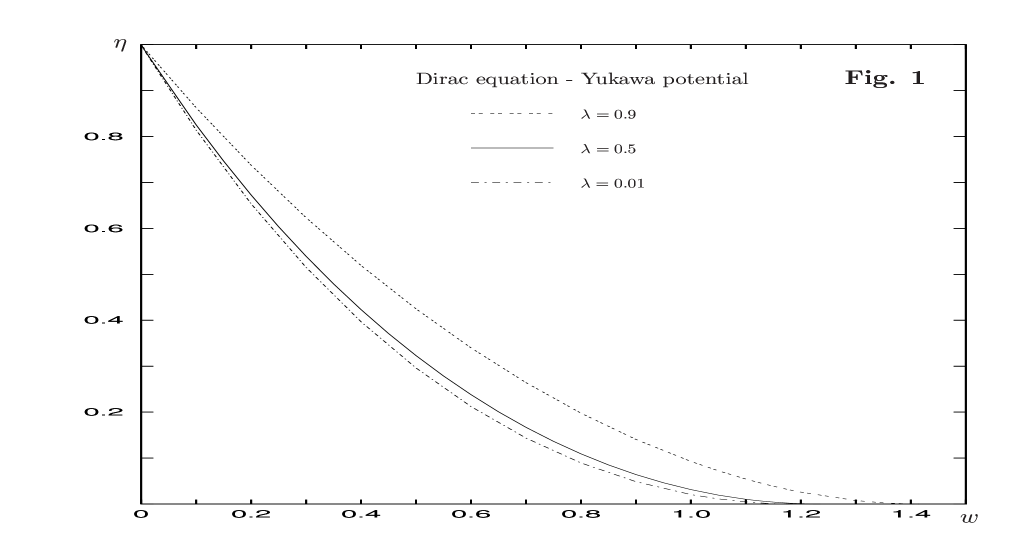
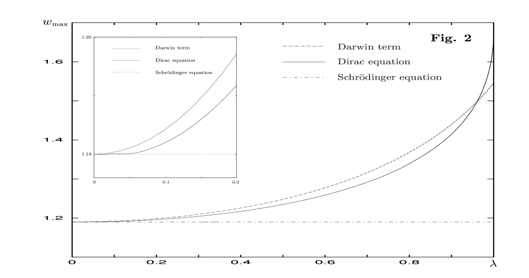
Figure 1: $\eta$ versus $\omega$ for the ground state of the Yukawa potential in the Dirac equation. Three values of $\lambda$ are shown. For $\lambda\ll 1$ (the dot-dash curve) we reproduce essentially the Schrödinger equation result. The value of $w_{\mbox{\tiny max}}$ when $\eta=0$ shows an increase with increasing $\lambda$.

Figure 2: Comparison of $w_{\mbox{\tiny max}}$ against $\lambda$ for the ground state in the Dirac and Schrödinger equations. The dashed curve is the magnification effect of the Yukawa version of the Darwin term alone.

References

- [1] S. Fukuda et al. (Super-Kamiokande), Phys. Rev. Lett. 86, 5656 (2001); Q. R. Ahmad et al. (SNO) Phys. Rev. Lett. 87, 071301 (2001), ibidem 89, 011301 (2002); K. Eguchi et al.(KamLAND) Phys. Rev. Lett. 90, 021802 (2003); M. H. Ahn et al. (K2K) Phys. Rev. Lett. 90, 041801 (2003).
- [2] S. Flügge, Practical Quantum Mechanics (Springer-Verlag, Berlin, 1999).
- [3] C. Cohen-Tannoudji, B. Diu and F. Laloë, Quantum Mechanics (John Wiley Sons, Paris, 1977).
- [4] O. Klein, Z. Phys. 53, 157 (1929).
- [5] A. Calogeracos and N. Dombey, Int. J. Mod. Phys. A 14, 631 (1999); Phys. Rept. 315, 41 (1999).
- [6] K. Kagiwara et al., Phys. Rev. D 66, 010001 (2002).
- [7] S. H. Patil, J. Phys. A 34, 3153 (2001).
- [8] G. Jian-You, F. X. Zheng, and X. Fu-Xin. Ch. Phys. Lett, 20, 602 (2003).
- [9] A. D. Alhaidari, Pys. Rev. Lett. 87, 210405 (2001).
- [10] F. Gross, Relativistic Quantum Mechanics and Field Theory ( John Wiley Sons, New York, 1993).
- [11] L. L. Foldy and S. A. Wouthuysen, Phys. Rev. 78, 29 (1950).
- [12] J. J. Sakurai, Advanced Quantum Mechanics (Addison-Wesley, New York, 1987) .
- [13] H. A. Bethe and E. E. Salpeter, Quantum Mechanics of One and Two Electron Atoms (Springer-Verlag, Berlin, 1957).