Quantum Gravity and Property of the very early Universe

Abstract

As is well known, the universally accepted theory as quantum gravity (QG) doesn’t exist. One of the main reasons for that is that quantized general relativity is perturbatively nonrenormalizable. But there are several theories whose low-energy effective action is general relativity such as super string theory, supergravity and so on. On the other hand there is the prospect that quantized general relativity will become consistent nonperturbatively, for example by way of the $\epsilon$ - expanded analysis in 2 + $\epsilon$ gravity and the implication of the exact renormalization group equation (ERGE) and so on. Thus, the reason that we can’t check which is right, is because of no constraint from experiments. By the way, the early Universe can be considered a good laboratory for QG, because of the high energy scale. In this period it is thought that the effect of QG governed the Universe. Therefore to construct the Universe model out of consideration of a certain type of QG can be thought of the test of the theory. Here the result of quantized general relativity, which is treated nonperturbatively by ERGE, is checked. The application of QG improved Einstein equation to the very early Universe shows several characteristic properties. At first the Universe become free from the initial singularity. The second is the origin of the cosmological time is uniquely decided. Furthermore this result doesn’t destroy the success that the current cosmology attained.

I Introduction

General relativity proposed by Einstein in 1915 can explain successfully the macroscopic properties of gravity. Nevertheless the effort trying to quantize general relativity failed because of the perturbative nonrenormalizability. Which is to say we can’t control the divergence of perturbatively quantized general relativity. As the result, general relativity is thought of as the only effective theory of a fundamental theory defined on higher energy scale. For example, super string theory and supergravity were proposed as such a theory. But it is shown that these theories are also perturbatively nonrenormalizable Deser . On the other hand there is the prospect that quantized general relativity will become consistent nonperturbatively. By this means the $\epsilon$ - expanded analysis in 2 + $\epsilon$ gravity Kawai and the implication of the ERGE Reuter Souma showed that quantized general relativity is nonperturbatively renormalizable according to the asymptotic safety that was put forward by Weinberg Weinberg . This idea is that the quantum theory which lies on the ultraviolet critical surface of some ultraviolet fixed point is renormalizable. Thus several theories of QG exist, but an universally accepted one is absent. the reason of persisting in this situation is mainly because the constraints from experiments don’t exist.

Currently, the measurements by cosmic microwave background (CMB) spectral, Type Ia supernovae observation and so on are consistent with an infinite flat universe containing about 30% cold dark matter, 65% dark energy and 5% ordinary matter. Furthermore many observations are going to clarify the current and past Universe. In the circumstances the early Universe can be considered a good laboratory for QG. One of the reasons is to think that the Universe experienced the period such as immediately after the big bang in which QG effects dominated. And the trace of QG effects may be observed by the current precision measurements. Therefore to construct the Universe model out of consideration of a certain type of QG can be thought of as the test of the theory. If the model can explain some of the problems of modern cosmology such as the horizon and flatness problems, the cosmological constant problem, the one of the construction of the large scale structure, the identity of the dark matter and energy and so on, it is thought of as the suggestive matter to believe that the theory is correct.

Here the very early Universe is considered in according to the result by the analysis of the ERGE of quantized general relativity. This idea is also an approximate one to justify the present situation that the classical general relativity is used to the study of the early Universe and inflation mechanism and so on, because the analysis of the ERGE assure that general relativity is the fundamental theory.

In the next section the ERGE formalism for QG by Reuter is reviewed in brief. In section 3 the properties of QG in light of the ERGE analysis are described. In section 4 the applications of QG to the very early Universe and the behavior of the QG improved Universe are discussed. Section 5 is devoted to the conclusion.

II Formulation of Exact Renormalization Group Equation for QG

II.1 Quantization of Gravity

In this subsection the Lagrangian of gravity ${\cal L}_{\rm GR}$ which is the general functional of the metric $\gamma_{\mu\nu}$ is considered. Then the classical action of gravity $S_{\rm GR}$ is invariant under the local general coordinate transformation. $S_{\rm GR}$ is quantized in a fixed Euclidean background field in $d$ dimensions. The metric $\gamma_{\mu\nu}$ is decomposed as $\gamma_{\mu\nu}=\bar{g}_{\mu\nu}+h_{\mu\nu}$. Here, $\bar{g}_{\mu\nu}$ denotes a fixed Euclidean background field and $h_{\mu\nu}$ denotes the fluctuations around the background. Now the general coordinate transformation is given by

$$\delta h_{\mu\nu} = \pounds_{v}\gamma_{\mu\nu}=v^{\rho}\partial_{\rho}\gamma_{\mu\nu}+\partial_{\mu}v^{\rho}\cdot\gamma_{\rho\nu}+\partial_{\nu}v^{\rho}\cdot\gamma_{\mu\rho}$$ (1)

$$\equiv \nabla_{\mu}v_{\nu}+\nabla_{\nu}v_{\mu},$$

$$\delta\bar{g}_{\mu\nu} = 0,$$ (2)

where $\pounds_{v}$ denotes the Lie derivative with respect to the vector field $v^{\mu}$. Because the local general coordinate transformation is a kind of gauge transformation, to fix the gauge the BRST symmetry is introduced. The BRST transformation of the gravitation field $h_{\mu\nu}$ is given by

$$\mbox{\boldmath$\delta$}_{\bf B}h_{\mu\nu}=\kappa^{-2}\pounds_{C}\gamma_{\mu\nu}.$$ (3)

Here $C_{\mu\nu}$ denotes the ghost field and $\mbox{\boldmath$\delta$}_{\bf B}$ is an anticommuting operator of the BRST transformation. In addition $\kappa$ is a constant expressed in terms of the bare Newton constant $\bar{G}$ as $\kappa=(32\pi\bar{G})^{-1/2}$. The transformation of the other fields are given by

$$\mbox{\boldmath$\delta$}_{\bf B}\bar{g}_{\mu\nu} = 0,$$

$$\mbox{\boldmath$\delta$}_{\bf B}C^{\mu} = \kappa^{-2}C^{\nu}\partial_{\nu}C^{\mu},$$

$$\mbox{\boldmath$\delta$}_{\bf B}\bar{C}_{\mu} = B_{\mu},$$

$$\mbox{\boldmath$\delta$}_{\bf B}B_{\mu} = 0,$$ (4)

where $\bar{C}_{\mu}$ and $B_{\mu}$ denote the anti-ghost field and the auxiliary field, respectively. Then the gauge fixing Lagrangian and the Faddeev - Popov ghost Lagrangian are introduced by

$${\cal L}_{\rm GF} = \kappa B_{\mu}(F^{\mu}+\frac{\alpha\kappa}{2}B^{\mu}),$$

$${\cal L}_{\rm GH} = -\kappa\bar{C}_{\mu}(\mbox{\boldmath$\delta$}F^{\mu}).$$

Here $F_{\mu}$ is defined to become linear with respect to $h_{\mu\nu}$ as

$$F_{\mu}=\sqrt{2}\kappa{\cal F}^{\rho\sigma}_{\mu}[\bar{g}]h_{\rho\sigma},\qquad{\cal F}^{\rho\sigma}_{\mu}=\delta^{\rho}_{\mu}\bar{D}^{\sigma}-\frac{1}{2}\bar{g}^{\rho\sigma}\bar{D}_{\mu},$$

then the gauges are fixed to the harmonic gauge. Here $\bar{D}$ is the covariant derivative with respect to $\bar{g}_{\mu\nu}$ and $\alpha$ denotes the gauge parameter.

Now the generating functional for the connected Green’s function is given by

$$W[{\rm ES};\bar{g}]=\ln\int{\cal D}\Phi\exp[-S[\Phi;\bar{g}]-S_{\rm ES}],$$ (5)

where the subscript ES denotes external sources and $\Phi=\{h,C,\bar{C}\}$ is the shorthand notation. Here the classical action $S[\Phi;\bar{g}]$ is given by

$$S[\Phi;\bar{g}]=S_{\rm GR}[h;\bar{g}]+S_{\rm GF}[h;\bar{g}]+S_{\rm GH}[\Phi;\bar{g}],$$ (6)

$$S_{\rm GR}[h;\bar{g}] = \int d^{d}x{\cal L}_{\rm GR}[\bar{g}+h],$$ (7)

$$S_{\rm GF}[h;\bar{g}] = \frac{1}{2\alpha}\int d^{d}x\sqrt{\bar{g}}\bar{g}^{\mu\nu}F_{\mu}F_{\nu},$$ (8)

$$S_{\rm GH}[\Phi;\bar{g}] = -\sqrt{2}\int d^{d}x\sqrt{\bar{g}}\bar{C}_{\mu}(\delta^{\mu}_{\nu}\bar{D}^{2}+\bar{R}^{\mu}_{\ \nu})C^{\nu}.$$ (9)

In addition note that $B$ integral has still completed and $\bar{R}^{\mu}_{\ \nu}$ denotes Ricci tensor with respect to $\bar{g}_{\mu\nu}$.

II.2 Average Action of Gravity

First $t^{\mu\nu},\bar{\sigma}_{\mu},\sigma^{\mu}$ and $\beta^{\mu\nu},\tau_{\mu}$ are introduced as the external sources that couple with $h_{\mu\nu},C^{\mu},\bar{C}_{\mu}$ and the BRST transformation of gravitation and ghost fields respectively. Then the scale dependent generating functional for the connected Green’s function $W_{k}$ is expressed as

$$W_{k}[J;\beta,\tau;\bar{g}_{\mu\nu}]=\ln\int{\cal D}\Phi\exp[-S[\Phi;\bar{g}]-\Delta S_{k}[\Phi;\bar{g}]-S_{\rm ES}]$$ (10)

in terms of the shorthand notation $J=\{t,\bar{\sigma},\sigma\}$. Here k is an arbitrary momentum infrared cutoff scale that satisfies $k\leq\Lambda$, $\Lambda$ is a physical ultraviolet cutoff which is associated with the classical action of the theory. In addition the external source action $S_{\rm ES}$ and the cutoff action $\Delta S_{k}[\Phi;\bar{g}]$ are given by

$$S_{\rm ES} = -\int d^{d}x\sqrt{\bar{g}}[J\Phi+\beta^{\mu\nu}\pounds_{C}(\bar{g}_{\mu\nu}+h_{\mu\nu})+\tau_{\mu}C^{\nu}\partial_{\nu}C^{\mu}],$$ (11)

$$\Delta S_{k}[\Phi;\bar{g}] = \frac{1}{2}\kappa^{2}\int d^{d}x\sqrt{\bar{g}}h_{\mu\nu}(R_{k}^{\rm grav}[\bar{g}])^{\mu\nu\rho\sigma}h_{\rho\sigma}+\sqrt{2}\int d^{d}x\sqrt{\bar{g}}\bar{C}_{\mu}(R_{k}^{\rm gh}[\bar{g}])C^{\mu},$$ (12)

respectively. The cutoff function $R_{k}[\bar{g}]$ is expressed in terms of the dimensionless cutoff function $R^{(0)}(u)$ as

$$R_{k}^{grav}[\bar{g}] = Z_{k}^{\rm grav}k^{2}R^{(0)}(-\bar{D}^{2}/k^{2}),$$

$$R_{k}^{gh}[\bar{g}] = Z_{k}^{\rm gh}k^{2}R^{(0)}(-\bar{D}^{2}/k^{2}).$$

$R^{(0)}(u)$ is arbitrary function which decides the property of the cutoff scheme and must interpolate smoothly between $R^{(0)}(0)=1$ and $R^{(0)}(u\rightarrow\infty)=0$. In addition $Z_{k}^{\rm grav}$ and $Z_{k}^{\rm gh}$ denote the renormalization factors of the gravitation field and the ghost field ,respectively. In particular $Z_{k}^{\rm grav}$ is the tensor with respect to the background metric and is given by $(Z_{k}^{\rm grav})^{\mu\nu\rho\sigma}=\bar{g}^{\mu\rho}\bar{g}^{\nu\sigma}Z_{k}^{\rm grav}$ as the simplest case. Then classical fields $\bar{h}_{\mu\nu},\xi^{\mu},\bar{\xi}_{\mu}$ are given by

$$\bar{h}_{\mu\nu}=\frac{1}{\sqrt{\bar{g}}}\frac{\delta W_{k}}{\delta t^{\mu\nu}},\qquad\xi^{\mu}=\frac{1}{\sqrt{\bar{g}}}\frac{\delta W_{k}}{\delta\bar{\sigma}_{\mu}},\qquad\bar{\xi}_{\mu}=\frac{1}{\sqrt{\bar{g}}}\frac{\delta W_{k}}{\delta\sigma^{\mu}},$$ (13)

respectively. Thus the average action of gravity is decided by using the modified Legendre transformation as

$$\Gamma_{k}[\bar{h},\xi,\bar{\xi};\beta,\tau;\bar{g}] = -W_{k}[J;\beta,\tau;\bar{g}]+\int d^{d}x\sqrt{\bar{g}}[t^{\mu\nu}\bar{h}_{\mu\nu}+\bar{\sigma}_{\mu}\xi^{\mu}+\sigma^{\mu}\bar{\xi}_{\mu}]-\Delta S_{k}[\bar{h},\xi,\bar{\xi};\bar{g}]$$ (14)

$$\equiv \widetilde{\Gamma}_{k}[\bar{h},\xi,\bar{\xi};\beta,\tau;\bar{g}]-\Delta S_{k}[\bar{h},\xi,\bar{\xi};\bar{g}].$$

Then the classical metric $g_{\mu\nu}$ which is the counterpart of the quantum metric $\gamma_{\mu\nu}$ is defined as

$$g_{\mu\nu}(x)\equiv\bar{g}_{\mu\nu}(x)+\bar{h}_{\mu\nu}(x).$$ (15)

From now the average action is expressed in terms of $g_{\mu\nu}$ instead of $\bar{h}$ as

$$\Gamma_{k}[\bar{h},\xi,\bar{\xi};\beta,\tau;\bar{g}] = \Gamma_{k}[g-\bar{g},\xi,\bar{\xi};\beta,\tau;\bar{g}]$$ (16)

$$\equiv \Gamma_{k}[g,\bar{g},\xi,\bar{\xi};\beta,\tau].$$

II.3 Evolution Equation of Gravity

Differentiating Eq.(14) with respect to $t=\ln(k/\Lambda)$, and after some calculations the evolution equation of gravity is given by

$$\partial_{t}\Gamma_{k} = \frac{1}{2}{\rm Tr}\left[\left(\Gamma_{k}^{(2)}+\kappa^{2}R_{k}^{\rm grav}\right)_{\bar{h}\bar{h}}^{-1}\left(\partial_{t}(\kappa^{2}R_{k}^{\rm grav})\right)_{\bar{h}\bar{h}}\right]$$ (17)

$$-\frac{1}{2}{\rm Tr}\left[\left\{\left(\Gamma_{k}^{(2)}+\sqrt{2}R_{k}^{\rm gh}\right)_{\bar{\xi}\xi}^{-1}-\left(\Gamma_{k}^{(2)}+\sqrt{2}R_{k}^{\rm gh}\right)_{\xi\bar{\xi}}^{-1}\right\}\left(\partial_{t}(\sqrt{2}R_{k}^{\rm gh})\right)_{\bar{\xi}\xi}\right].$$

Here ${\rm Tr}=\sum\int d^{d}x\sqrt{\bar{g}}\int d^{d}y\sqrt{\bar{g}}$ and $\sum$ denotes to figure out the sum with respect to the indices both of the gravitation and ghost fields.$\Gamma_{k}^{(2)}$ is the Hessian of $\Gamma_{k}$ with respect to the subscript. In addition this evolution equation must satisfy as the initial condition the average action at the physical UV cutoff scale $\Gamma_{\Lambda}$ which is given by

$$\Gamma_{\Lambda}[g,\bar{g},\xi,\bar{\xi};\beta,\tau] = S_{\rm GR}[g-\bar{g};\bar{g}]+S_{\rm GF}[g-\bar{g};\bar{g}]+S_{\rm GH}[g-\bar{g},\xi,\bar{\xi};\bar{g}]$$ (18)

$$-\int d^{d}x\sqrt{\bar{g}}[\beta^{\mu\nu}\pounds_{\xi}g_{\mu\nu}+\tau_{\mu}\xi^{\nu}\partial_{\nu}\xi^{\mu}].$$

II.4 Gauge Invariant theory space

In general the ERGE formulation of the gauge theory can’t conserve the gauge symmetry explicitly, because it involves the cutoff. So in an ordinary way, to make only the observable gauge invariant is as best we can. In other words the effective action $\Gamma\equiv\lim_{k\rightarrow 0}\Gamma_{k}$ must be brought to satisfy the Ward - Takahashi equation. Now this requirement leads the next condition.

$$0 = \langle\mbox{\boldmath$\delta$}_{\bf B}\Delta S_{k}+\mbox{\boldmath$\delta$}_{\bf B}S_{\rm ES}\rangle$$ (19)

$$= \Bigl{\langle}\mbox{\boldmath$\delta$}_{\bf B}\Delta S_{k}-\int d^{d}x\sqrt{\bar{g}}J(\mbox{\boldmath$\delta$}_{\bf B}\Phi)\Bigr{\rangle}$$

Rewriting this condition in terms of the average action $\Gamma_{k}$ and after some calculations, so-called the modified Ward - Takahashi equation is obtained as

$$\int d^{d}x\frac{1}{\sqrt{\bar{g}}}\left[\frac{\delta\Gamma_{k}}{\delta\bar{h}_{\mu\nu}}\frac{\delta\Gamma_{k}}{\delta\beta^{\mu\nu}}+\frac{\delta\Gamma_{k}}{\delta\xi^{\mu}}\frac{\delta\Gamma_{k}}{\delta\tau_{\mu}}\right]=Y_{k}.$$ (20)

Here $Y_{k}$ become complicated expression as the follows

$$Y_{k} = \kappa^{2}{\rm Tr}\left[(R_{k}^{\rm grav})^{\mu\nu\rho\sigma}(\Gamma_{k}^{(2)}+\kappa^{2}R_{k}^{\rm grav})_{\bar{h}_{\rho\sigma}\varphi}^{-1}\frac{\delta^{2}\Gamma_{k}}{\sqrt{\bar{g}}\delta\varphi\sqrt{\bar{g}}\delta\beta^{\mu\nu}}\right]$$

$$-\sqrt{2}{\rm Tr}\left[R_{k}^{\rm gh}(\Gamma_{k}^{(2)}+\sqrt{2}R_{k}^{\rm gh})_{\xi^{\mu}\varphi}^{-1}\frac{\delta^{2}\Gamma_{k}}{\sqrt{\bar{g}}\delta\varphi\sqrt{\bar{g}}\delta\tau_{\mu}}\right]$$

$$+2\alpha^{-1}\kappa^{2}{\rm Tr}\left[R_{k}^{\rm gh}{\cal F}^{\rho\sigma}_{\mu}(\Gamma_{k}^{(2)}+\kappa^{2}R_{k}^{\rm grav})_{\bar{h}_{\rho\sigma}\bar{\xi}_{\mu}}^{-1}\right],$$

where $\varphi=\{\bar{h},\xi,\bar{\xi}]\}$ is a shorthand notation of the classical fields set. Then $Y_{k}$ goes to zero as $k\rightarrow 0$ because of $R_{k}^{\rm grav}=R_{k}^{\rm gh}=0$ in this limit. That is to say it insures that the effective action $\Gamma_{k\rightarrow 0}$ satisfy the usual Ward - Takahashi equation. By the way the exact solution of the evolution equation (17) satisfy the modified Ward - Takahashi equation (20), of course. But there is no guarantee that the approximate solutions of Eq.(17) do so. Therefore the solution space that satisfy the Eq.(20) is called the gauge invariant space and used as the indicator of approximate quality. Note that the gauge invariant space is different from the space which is spanned by all the gauge invariant operator.

II.5 Approximation of Evolution Equation

To solve the evolution equation(17) the infinite theory space must be truncated to the adequate subspace. As first approximation, the following subspace is considered.

1. The evolution of both the ghost action and external sources are neglected. As a result, $S_{\rm GF}$ and $S_{\rm GH}$ in $\Gamma_{k}$ are in the same form as that in the bare action.

2. $\Gamma_{k}$ is decomposed formally as

   $$\Gamma_{k}[g,\bar{g},\xi,\bar{\xi};\beta,\tau] = \bar{\Gamma}_{k}[g]+\hat{\Gamma}_{k}[g,\bar{g}]+S_{\rm GF}[g-\bar{g};\bar{g}]+S_{\rm GH}[g-\bar{g},\xi,\bar{\xi};\bar{g}]$$ (21)

   $$-\int d^{d}x\sqrt{\bar{g}}[\beta^{\mu\nu}\pounds_{\xi}g_{\mu\nu}+\tau_{\mu}\xi^{\nu}\partial_{\nu}\xi^{\mu}],$$

   where $\bar{\Gamma}_{k}[g]\equiv\Gamma_{k}[g,g,0,0;0,0]$ and $\hat{\Gamma}_{k}$ contains the deviations for $g_{\mu\nu}\neq\bar{g}_{\mu\nu}$ so that $\hat{\Gamma}_{k}[g,g]=0$. $\hat{\Gamma}_{k}$ can be interpreted as the quantum corrections to $S_{\rm GF}$, so $\hat{\Gamma}_{k}=0$ for all $k$ become a candidate for the first approximation. Of course, this ansatz satisfies the initial condition (18).

In addition it is sure that this approximated subspace is the gauge invariant space, because of $\hat{\Gamma}_{k}[g,\bar{g}]=0$. Here $Y_{k}$ is given by

$$Y_{k}=-\int d^{d}x\pounds_{\xi}g_{\mu\nu}\frac{\delta\hat{\Gamma}_{k}[g,\bar{g}]}{\delta g_{\mu\nu}(x)}.$$

Now inserting the approximated average action (21) into Eq.(17), the evolution equation in the gauge invariant theory space is given by

$$\partial_{t}\Gamma_{k}[g,\bar{g}] = \frac{1}{2}{\rm Tr}\left[(\kappa^{-2}\Gamma_{k}^{(2)}[g,\bar{g}]+R_{k}^{\rm grav}[\bar{g}])^{-1}(\partial_{t}R_{k}^{\rm grav}[\bar{g}])\right]$$ (22)

$$-{\rm Tr}\left[\left(-(\delta^{\mu}_{\nu}D^{2}+R^{\mu}_{\ \nu})+R_{k}^{\rm gh}[\bar{g}]\right)^{-1}(\partial_{t}R_{k}^{\rm gh}[\bar{g}])\right].$$

Here,

$$\Gamma_{k}[g,\bar{g}]\equiv\Gamma_{k}[g,\bar{g},0,0;0,0]=\bar{\Gamma}_{k}[g]+S_{\rm GF}[g-\bar{g};\bar{g}],$$ (23)

where $D$ and $R_{\mu\nu}$ are the covariant derivative and Ricci tensor with respect to $g_{\mu\nu}$, respectively.

II.6 Einstein - Hilbert Truncation

Eq.(22) is still too difficult to solve actually. So to make the problem easier, the theory space is constrained moreover. At first, to take the classical action $S_{\rm GR}$ as the Einstein - Hilbert action will be the simplest approximation. Einstein - Hilbert action is given by

$$S_{\rm GR}=\frac{1}{16\pi\bar{G}}\int d^{d}x\sqrt{g}\left[-R(g)+2\bar{\lambda}\right]=2\kappa^{2}\int d^{d}x\sqrt{g}\left[-R(g)+2\bar{\lambda}\right].$$ (24)

Here $\bar{G}$ and $\bar{\lambda}$ are the bare Newton constant and bare cosmological constant, respectively. These bare constants are rewrote to the scale dependent couplings in light of the field renormalization factor as

$$\bar{G}\rightarrow\bar{G}_{k}=\frac{1}{Z_{Nk}}\bar{G},\quad\bar{\lambda}\rightarrow\bar{\lambda}_{k}.$$

In addition to assign the scale dependence of gauge parameter $\alpha$ as

$$\alpha\rightarrow\alpha_{k}=\frac{1}{Z_{Nk}}\alpha.$$

Then the approximated average action becomes

$$\Gamma_{k}[g,\bar{g}] = 2\kappa^{2}Z_{Nk}\int d^{d}x\sqrt{g}\Big{[}-R(g)+2\bar{\lambda}_{k}\Big{]}$$ (25)

$$+\kappa^{2}Z_{Nk}\int d^{d}x\sqrt{\bar{g}}\bar{g}^{\mu\nu}({\cal F}^{\alpha\beta}_{\mu}g_{\alpha\beta})({\cal F}^{\rho\sigma}_{\nu}g_{\rho\sigma}).$$

Here note that $\kappa=(32\pi\bar{G})^{-1/2}$ is an independent constant of $k$ and gauge parameter is fixed to one. Then differentiating Eq.(25) with respect to $t$ and applying the condition $g_{\mu\nu}=\bar{g}_{\mu\nu}$ in order to delete the gauge fixing term. At last extracting the system of differential equations about $Z_{Nk}$ and $\bar{\lambda}_{k}$, the $\beta$ - functions of gravity are obtained.

II.7 $\beta$-Functions of Gravity

In according to the above discussions, in light of the dimensionless couplings of the Newton constant $g_{k}$ and the cosmological constant $\lambda_{k}$ defined as

$$g_{k} = k^{d-2}\bar{G}_{k}=k^{d-2}Z_{Nk}^{-1}\bar{G},$$

$$\lambda_{k} = k^{-2}\bar{\lambda}_{k},$$

the $\beta$ - functions of gravity are given by

$$\partial_{t}g_{k} = [d-2+\eta(k)]g_{k}$$ (26)

$$\partial_{t}\lambda_{k} = -[2-\eta(k)]\lambda_{k}$$ (27)

$$+ \frac{1}{2}g_{k}(4\pi)^{1-d/2}\left[2d(d+1)\Phi^{1}_{d/2}(-2\lambda_{k})-d(d+1)\eta(k)\tilde{\Phi}^{1}_{d/2}(-2\lambda_{k})-8d\Phi^{1}_{d/2}(0)\right].$$

Here and after the bars are omitted due not to confuse and the anomalous dimension $\eta(k)$ is given by

$$\eta(k)=\frac{g_{k}B_{1}(d,\lambda_{k})}{1-g_{k}B_{2}(d,\lambda_{k})},$$ (28)

$$B_{1}(d,\lambda_{k}) = \frac{1}{3}(4\pi)^{1-d/2}\Big{[}d(d+1)\Phi_{d/2-1}^{1}(-2\lambda_{k})-6d(d-1)\Phi_{d/2}^{2}(-2\lambda_{k})$$

$$-4d\Phi_{d/2-1}^{1}(0)-24\Phi_{d/2}^{2}(0)\Big{]},$$

$$B_{2}(d,\lambda_{k}) = -\frac{1}{6}(4\pi)^{1-d/2}\left[d(d+1)\tilde{\Phi}_{d/2-1}^{1}(-2\lambda_{k})-6d(d-1)\tilde{\Phi}_{d/2}^{2}(-2\lambda_{k})\right].$$

Here $\Phi$s are defined as the integral functions of the arbitrary dimensionless cutoff function $R^{(0)}$ as

$$\Phi_{n}^{p}(w) = \frac{1}{\Gamma(n)}\int_{0}^{\infty}dzz^{n-1}\frac{R^{(0)}(z)-zR^{(0)}{}^{\prime}(z)}{[z+R^{(0)}(z)+w]^{p}},$$

$$\tilde{\Phi}_{n}^{p}(w) = \frac{1}{\Gamma(n)}\int_{0}^{\infty}dzz^{n-1}\frac{R^{(0)}(z)}{[z+R^{(0)}(z)+w]^{p}},$$

and satisfy

$$\Phi_{n}^{p}(w)=\tilde{\Phi}_{n}^{p}(w)=\frac{1}{(1+w)^{p}}\qquad{\rm as}\qquad n\rightarrow 0.$$

III Property of QG

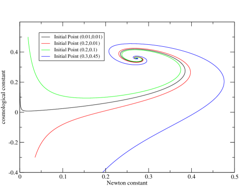
Figure 1: The numerically calculated flows of the $\beta$ - functions for the Newton constant and the cosmological constant in four dimensions. The initial points in the figure denote the only starting points to draw the associated flows, so don’t have the physical significance.

Fig.1 shows the numerically calculated flows of Eqs.(26) and (27) in four dimensions on the plane that is spanned by the $\sqrt{g}$ and $\sqrt{g}R$ operators. Explicitly two fixed point exist, these are an ultraviolet non - Gaussian fixed point (NGFP) and an infrared Gaussian fixed point (GFP). In particular the NGFP is attractive in the all directions as energy scale grows. This behavior is considered as the suggestion that $\sqrt{g}$ - $\sqrt{g}R$ plane is the subspace of the ultraviolet critical surface. In this way according to the asymptotic safe argument, quantized general relativity in four dimension is expected to be renormalizable nonperturbatively. It is known that this structure is maintained even if the matter fields are included Percacci , or $\sqrt{g}R^{2}$ term is taken into account.

In ultraviolet limit, in which is considered as the state of the very early Universe, the behaviors both of the Newton constant and the cosmological constant is uniquely controlled by the ultraviolet NGFP. That is to say that in neighborhood of the NGFP the dimensionful Newton constant $G_{k}$ and cosmological one $\lambda_{k}$ behave $G_{k}=g^{*}/k^{\epsilon}$ and $\lambda_{k}=\lambda^{*}k^{\epsilon}$ in $2+\epsilon$ dimensions, respectively. Here $g^{*}$ and $\lambda^{*}$ are the values of the dimensionless Newton constant and the cosmological one at the ultraviolet NGFP, respectively. Especially in four dimensions $G_{k}=g^{*}/k^{2}$ denotes that QG is asymptotic free.

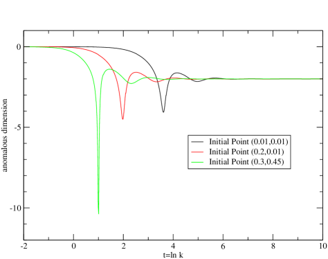
Figure 2: The numerically calculated result of the anomalous dimension from the $\beta$ - functions in four dimensions. The initial points in the figure are the same as Fig.1.

On the other hand, in infrared region the dimensionful Newton constant $G_{k}$ behave the same as the classical general relativity exactly because of the anomalous dimension $\eta=0$ that is showed by Fig.2. But the same time the property of the dimensionful cosmological constant can’t be controlled. It is thought as the disadvantage in light of the cosmological constant problem.

About the formalism used in this paper, the cutoff scheme dependence and the gauge parameter dependence are reported Reuter2 Souma2 . These may break the structure of the flow for the $\beta$ - functions. To solve these problems it is necessary the further investigation to include the other operators such as $\sqrt{g}R^{2}$ term and to consider the running gauge parameter in the approximate scheme and so on.

IV Application to the very Early Universe

In this section the result of the ERGE analysis for QG is applied the Robertson - Walker metric

$$ds^{2}=-dt^{2}+a^{2}(t)\left[\frac{dr^{2}}{1-Kr^{2}}+r^{2}(d\theta^{2}+\sin^{2}\theta d\phi^{2})\right],$$ (29)

which represents the homogeneous and isotropic Universe. Here $a(t)$ is the cosmological time $t$ dependent scale factor and $K$ is the curvature of the Universe. Though the time dependence of $a(t)$ follows the Einstein equation, to decide the dependence in the very early Universe the quantum effects of QG must be considered. The above ERGE analysis of QG indicates that the Newton constant $G$ and the cosmological constant $\Lambda$ in the classical Einstein equation must be treated as the scale dependent variables $G(k)$, $\Lambda(k)$. Therefore the ERGE modified Einstein equation is given by

$$G^{\mu}_{\ \nu}+\Lambda(k)\delta^{\mu}_{\ \nu}=8\pi G(k)T^{\mu}_{\ \nu},$$ (30)

$$T^{\mu}_{\ \nu}\equiv(-\rho,p,p,p),$$ (31)

where $T^{\mu}_{\ \nu}$ represents the energy - momentum tensor of the Universe as the ideal fluid. Here the behaviors of $G(k)$ and $\Lambda(k)$ in the very early Universe is considered as

$$G=g_{*}^{UV}/k^{2},$$ (32)

$$\Lambda=\lambda_{*}^{UV}k^{2},$$ (33)

in terms of the characteristic energy scale $k$ of a moment of the Universe. Secondly it is important how to identify the energy scale with the actual physical entity. Here I will introduce the energy scale related the actual geodesic distance. Namely, $k$ is expressed in terms of the comoving distance $x$ as

$$k=\xi/xa.$$ (34)

Here $\xi$ is a positive constant parameter. This identification has the advantage of that both the gravitational quantum effect observed in the today’s Universe and in the very early Universe are treated in the same framework. For example if a cosmological characteristic scale such as the scale of the cluster of galaxies is considered, the quantum effect is dominant at when the scale factor is small. On the other hand concerning a fixed scale factor the quantum effect manifests at the very short length. In according to this assumption, the equations for the evolution of the very early Universe are given by

$$\left(\frac{\dot{a}}{a}\right)^{2}=\frac{8\pi}{3}G(k)\rho-\frac{K}{a^{2}}+\frac{\Lambda(k)}{3},$$ (35)

$$G(k)\left(-\dot{\rho}-3\frac{\dot{a}}{a}(\rho+p)\right)-\dot{G}(k)\rho-\frac{\dot{\Lambda}(k)}{8\pi}=0,$$ (36)

$$G(k)=\widetilde{g_{*}}a^{2},\qquad\Lambda(k)=\widetilde{\lambda}_{*}/a^{2}.$$ (37)

Here $\widetilde{g_{*}}$ and $\widetilde{\lambda}_{*}$ are given by

$$\widetilde{g_{*}}=g_{*}^{UV}x^{2}/\xi^{2}\qquad,\qquad\widetilde{\lambda}_{*}=\lambda_{*}^{UV}\xi^{2}/x^{2},$$

with respect to a fixed comoving distance, respectively. Note that the scale dependences of the Newton constant and the cosmological constant are given by not hand but the ERGE analysis.

These equations (35), (36) represent the very early Universe as followings.

1. $a$ - $\rho$ relation
   The relation between the scale factor $a$ and the energy density $\rho$ of the Universe is derived from Eqs.(35) and (36). At first $K$, $\widetilde{g_{*}}$ and $\widetilde{\lambda}_{*}$ are defined as the appropriate constants. But five variables $(G,\Lambda,a,\rho,p)$ still remain whereas there are no more than four equations. Therefore the another equation must be given. Here though the relation is unknown, $\rho=wp$ is supposed as the equation of state. Then the relation between $a$ and $\rho$ is given by

   $$\frac{d\rho}{\rho}=(-3w-5)\frac{da}{a}+\frac{1}{4\pi}\frac{\widetilde{\lambda}_{*}}{\widetilde{g_{*}}}\frac{da}{a^{5}\rho}.$$ (38)

   Secondly substituting $\rho$ with $\bar{\rho}=4\pi(3w+5)\widetilde{g_{*}}\rho/\widetilde{\lambda}_{*}$ Eq.(38) becomes

   $$\frac{d\bar{\rho}}{da}=(3w+5)\left(-\frac{\bar{\rho}}{a}+\frac{1}{a^{5}}\right).$$ (39)

   

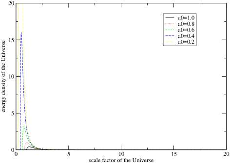
   Figure 3: The numerically calculated relation between $a$ and $\rho$ in $a\geq 0$ and $\bar{\rho}\geq 0$ region. Here $a0$ denotes the value of the scale factor at when the energy density of the Universe vanishes. In this figure $K=0$ and $w=0$ are used.

   This differential equation can be solved numerically in $a\geq 0$ and $\bar{\rho}\geq 0$ region, as a result Fig.3 is given. This result implies that if the quantum effect of QG is considered the energy density of the early Universe is free from the initial singularity.

2. $t$ - $a$ relation
   

   

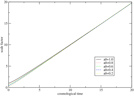
   Figure 4: The $t$ dependence of the scale factor $a$ in $t\geq 0$. Here $a0$ is the same as Fig.3, because of the uniquely determination of $t=0$. In this figure $K=0$ and $w=0$ are used, too.

   The cosmological time $t$ dependence of the scale factor $a$ is derived from Eqs.(35) and (38). Fig.4 gives the result. Here the requirement that $(da/dt)^{2}$ is kept positive in $\bar{\rho}\geq 0$ region with respect to the expansion of the Universe leads that the condition

   $$\frac{1}{3}-\frac{K}{\widetilde{\lambda}_{*}}\geq 0.$$ (40)

   If this is satisfied, the origin of the cosmological time $t=0$ can be determined uniquely at when the energy density of the Universe $\rho$ vanishes. Then the $t$ dependence of the scale factor in the very early Universe is considered as approximate linear because of Fig.5. This is different from the usual behavior of $a\propto\sqrt{t}$ in the radiation dominated period. As a result the horizon problem weakens, but to solve perfectly the other mechanism such as inflation is needed.

   

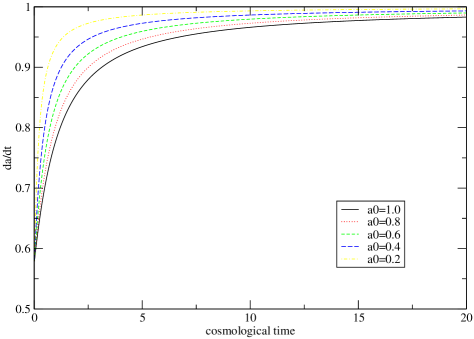
   Figure 5: The $t$ dependence of the gradient of the scale factor.

V Conclusion

In general to identify the energy scale is the most important task, if the result of ERGE analysis tries to apply the actual Universe. The ansatz Eq.(34) used in this paper is considered to work effectively at several points. As a result the ERGE modified Universe has the advantage of the followings.

• The Universe is free from the singularities.

• The origin of the cosmological time is uniquely decided.

In the next stage to solve the horizon and flatness problems and so on the other mechanics such as inflation is needed. Then this Universe is thought of as the credible framework in which the inflation mechanics are constructed and checked because of including the quantum effect explicitly.

By the way the several assumptions are used implicitly. They are that to apply the Euclidean ERGE results to the Minkowski Universe, to apply the pure gravity results to the Universe coupled with matter. These assumptions are necessarily to be investigated in detail.

At last the minimum scale factor of the Universe is natural decided. The ratio of this characteristic value to the current value of the scale factor is maybe related to Planck scale. Perhaps the origin of the quantum effect is also found in the very early Universe.

References

- (1) S.Deser, Annalen Phys. 9 (2000) 299-307
- (2) H.Kawai,M.Ninomiya, Nucl. Phys. B336 (1990) 115
- (3) M.Reuter, Phys. Rev. D57 (1998) 971
- (4) W.Souma, Prog.Theor.Phys. 102 (1999) 181-195
- (5) S.Weinberg, Ultraviolet divergences in quantum theories of gravitation, ed. S.Hawking and W.Israel(Cambridge Univ. Press,Cambridge 1979)
- (6) R.Percacci,D.Perini, Phys. Rev. D68 (2003) 044018
- (7) M.Reuter,F.Saueressig, Phys. Rev. D65 (2002) 065016
- (8) W.Souma, gr-qc/0006008