hep-th/0401031

MCTP-03-62

CPHT-RR-114-1203

IC/2003/162

MIT-CTP 3455

On the Universality Class of Certain String Theory Hadrons

G. Bertoldi¹, F. Bigazzi², A. L. Cotrone³, C. Núñez⁴, L. A. Pando Zayas⁵

¹ School of Natural Sciences, Institute for Advanced Study

Einstein Drive, Princeton, NJ 08540. USA

² The Abdus Salam ICTP, Strada Costiera, 11; I-34014 Trieste, Italy

³ CPHT, École Polytechnique, F-91128 Palaiseau Cedex, France

³INFN, Piazza dei Caprettari, 70; I-00186 Roma, Italy

⁴ Center for Theoretical Physics, MIT, Cambridge MA02140. USA

⁵ Michigan Center for Theoretical Physics

Randall Laboratory of Physics, The University of Michigan

Ann Arbor, MI 48109-1120. USA

Exploiting the gauge/gravity correspondence we find the spectrum of hadronic-like bound states of adjoint particles with a large global charge in several confining theories. In particular, we consider an embedding of four-dimensional ${\cal N}=1$ supersymmetric Yang-Mills into IIA string theory, two classes of three-dimensional gauge theories and the softly broken version of one of them. In all cases we describe the low energy excitations of a heavy hadron with mass proportional to its global charge. These excitations include: the hadron’s nonrelativistic motion, its stringy excitations and excitations corresponding to the addition of massive constituents. Our analysis provides ample evidence for the universality of such hadronic states in confining theories admitting supergravity duals. Besides, we find numerically a new smooth solution that can be thought of as a non-supersymmetric deformation of $G_{2}$ holonomy manifolds.

1 Introduction and Summary

The gauge/gravity correspondence has reached a new chapter with the realization of concrete scenarios where the correspondence can be taken beyond the supergravity approximation [1, 2]. An interesting example was given by Berenstein, Maldacena and Nastase who proposed a gauge theory interpretation of the Penrose-Güven limit for IIB supergravity on $AdS_{5}\times S^{5}$. A crucial ingredient in the BMN construction is that string theory in the resulting background is exactly soluble [3].

Inspired by this new insight, the authors of reference [4] considered a modification of the Penrose limit applicable to supergravity backgrounds dual to confining gauge theories. By focusing in on the IR region, exactly solvable string theory models were obtained. These string models represent in the gauge theory side the nonrelativistic motion and low-lying excitations of heavy hadrons with mass proportional to a large $U(1)$ global charge.

The hadronic states discussed in [4] are remarkable in that they are present in any confining theory admitting a supergravity dual. More precisely, as shown in [4], the conditions for the existence of a Penrose-Güven limit that focuses in on these states is compatible with the condition for a supergravity background to allow an area law for the VEV of a rectangular Wilson loop in the dual gauge theory.

In [4] the authors considered the Klebanov-Strassler (KS) [5] and the Maldacena-Núñez (MN) [6] backgrounds, both embeddings of 4-d ${\cal N}=1$ SYM into IIB string theory. The corresponding confining gauge theories consist of ${\cal N}=1$ SYM plus massive particles in the adjoint representation carrying a global $U(1)$ charge. After taking the Penrose limit it was realized that the string Hamiltonian on the resulting background describes stringy shaped hadrons, called annulons, which are bound states of these massive particles, in the limit where the charge and the number of colors both go to infinity.

The analysis of [4] attempts to elucidate which properties of the annulons are universal to any background dual to a confining theory and which depend on the particular embedding. Recently, softly broken versions of the KS and MN backgrounds were considered in [7, 8] with results very similar to those of [4].

In this paper we explore other string duals of confining gauge theories, and show how those universal properties are in fact manifest.

The first model we consider is an embedding of 4-d ${\cal N}=1$ SYM into IIA string theory. The field theory lives on the worldvolume of $N$ D6-branes wrapped on a three-cycle of a deformed conifold. The dual IIA background results in a product of a flat 4-d Minkowski space and a resolved conifold, and it is supported by $N$ units of RR two-form flux through the non vanishing two-cycle. This 10-d solution is obtained as a $U(1)$ compactification of an M-theory background with an asymptotically locally conical, $G_{2}$ holonomy metric [9, 10]. The circle along which we compactify has finite size everywhere; this ensures that the 10-d solution is regular.

As a second class of models, we consider IIB and IIA string duals to three dimensional ${\cal N}=1$ confining gauge theories. The relevant backgrounds were given in [11, 12, 13] and [14] respectively. In a sense they are the 3-d analogue of the MN and KS backgrounds. The solution in [13] describes the geometry generated by fivebranes wrapped over a three-cycle of a (topologically) $G_{2}$ holonomy manifold; recall that the MN background describes D5-branes wrapped on a two-cycle. The one in [14] corresponds to a stack of regular and fractional D2-branes whereas KS corresponds to a stack of D3 and fractional D3-branes. We also consider the gluino-mass-deformed version of the gauge model dual to the solution in [11, 12, 13]. The corresponding non supersymmetric background was studied in [15].

The understanding of 3-d gauge theories in the context of the AdS/CFT correspondence is less precise. In fact, the AdS/CFT correspondence has been used to predict various properties of confining 3-d gauge theories [16] . We thus present our analysis as an alternative way of gaining information about 3-d confining gauge theories. Having in some sense established the universality of certain states in embeddings of 4-d confining theories we proceed to study the corresponding states in 2+1 dimensions.

Finally, with the intention of exploiting a non supersymmetric version of the 4-d model above, we numerically find a new set of solutions that are non supersymmetric deformations of $G_{2}$ holonomy manifolds. These solutions are smooth and, depending on the range of parameters, we can attempt an interpretation as duals to D6-branes wrapping cycles in a non-supersymmetric fashion. The brane interpretation suggests that these solutions might be considered as new gravity duals of confining non supersymmetric gauge theories, though more work is needed to precisely state this conjecture. As a first plausibility indication we analyze the Penrose limit of the new backgrounds, finding a pp-wave solution identical to the one found in the susy case: this should give us some evidence about the presence of annulons also in this nonsupersymmetric context.

The paper is organized as follows. In the following section we give a general overview of the problem as well as a description of the main principle behind our analysis. Section 3 contains a description of our Penrose limit applied to the resolved conifold with RR two-form and the spectrum of IIA string theory on the resulting background. In section 4 we describe the Penrose limit of the D5-on-$S^{3}$ supersymmetric and softly broken solutions. Section 5 deals with the D2 and fractional D2-branes model. Section 6 contains our analysis of the string theory results from the gauge theory point of view. We identify the constituents of the ground state hadrons and the corresponding excitations. In section 7 we present the nonsupersymmetric deformation of the background studied in section 3. Section 8 contains some concluding remarks. We have also included a number of appendices that contain explicit calculations of technical statements made in the body of the paper. Appendix A contains standard expressions for the $SU(2)$ left-invariant forms and a parametrization of $\mathbb{R}^{4}$ used in the main body. Appendix B contains the fermionic string equations of motion for a generic plane wave background. The BPST instanton needed for the explicit form of the solution treated in section 5 is given explicitly in appendix C. Appendix D contains a discussion of the regularization used to compute the zero point energy of the string theories obtained in the main body. Appendix E presents the full set of second order differential equations that are solved in section 7 to obtain the new nonsupersymmetric deformation of the $G_{2}$ holonomy metric. This appendix also contain fifteen figures designed to present a graphical proof of the existence and properties of the new solution.

Reader’s guide: Since this is a long paper, it is useful to give a ‘road-book’ for readers with diverse interests. Those interested in the ‘geometrical’ aspects of the paper, like Penrose limits, pp-waves and non supersymmetric deformations of $G_{2}$ holonomy manifolds, should read sections 3.1, 4, 5.1, and section 7 (this last one can be read almost independently of the rest of the paper). Readers more concerned with string theory aspects of this work, should refer to sections 3.2, 3.3, 4.1, 5.2, 6 and appendix D.

2 Physical picture of the general idea

One of the main purpose of this paper is to address the universality of the annulons, i.e. those hadronic states first considered in [4].

A controlled setup in which to study gauge theory IR dynamics, including confinement, would be in the presence of supersymmetry. Four-dimensional ${\cal N}=1$ SYM provides such a system . In the context of the gauge/gravity correspondence this would correspond to studying the string theory dual to ${\cal N}=1$ SYM which is not known. The best we can do at the moment is to study supergravity backgrounds that correspond to confining gauge theories that contain ${\cal N}=1$ SYM as a sector. In all known cases these confining gauge theories contain massive fields that transform in the adjoint of the gauge group and have some global charge. If we group enough of these massive particles we might hope that they form bound states. This is precisely the field theoretic question we address: What is the spectrum of a collection of a large number of these massive, globally charged, adjoint particles?

The question just formulated about the spectrum of a bound state of adjoint particles with global charge is out of the reach of current field theoretic techniques. However, the gauge/gravity correspondence provides an exact answer.

The general principle allowing to address such questions in string theory was articulated by Gubser, Klebanov and Polyakov in [2]. In the gauge/gravity correspondence there is a direct relation between sectors of the gauge theory with large quantum numbers and classical solitonic solutions of the string sigma model on the corresponding supergravity background. Under this point of view the BMN sector of operators [1] corresponds to a string shrunk to a point and orbiting at the speed of light along the great circle of $S^{5}$. For BMN operators in the gauge theory, the R-charge is to be identified with the angular momentum of the classical solution. Applying this principle to the question at hand we can translate the spectrum of a bound state of a large number of globally charged massive adjoint particles into the semiclassical analysis of a macroscopic string that spins in the space perpendicular to the worldvolume of the gauge theory. The angular momentum of the classical string is to be identified with the global charge of the bound state. As shown in [4], such a string configuration can only be stationary in the region corresponding to the IR of the gauge theory. Thus the classical configuration we consider is a string stuck at the “minimal radius” and spinning in the internal space.

It is worth pointing out the role of this region for the states we describe. A hadron, being a gauge theory state of definite four-dimensional mass, is dual to a supergravity eigenstate of the ten- and four-dimensional Laplacians. In the world volume directions these states are plane waves. The wave function in the remaining directions falls off as $\psi(r,\Omega)\sim r^{-\Delta}$, where $\Delta$ is the dimension of the lowest-dimension operator which can create the hadron. Therefore, a hadron made of a large number of constituents is localized near the “minimal AdS radius.”

It is remarkable that for this particular configuration we can provide an exact analysis. The reason is that it can be studied by means of a particular Penrose limit. This effectively implies, as in the BMN case, that the semiclassical quantization is exact. The Penrose limit provides a truncation of the supergravity background to one in which the corresponding string theory can be exactly solved.

3 Resolved conifold with RR two-form flux

In this section we consider a IIA background argued to be dual to an embedding of ${\cal N}=1$ SYM into string theory. This background is a resolved conifold metric with RR two-form flux turned on over the blown up $S^{2}$.

The simplest interpretation of this background is as originating from a $G_{2}$ holonomy metric in the $D_{7}$ family [9, 10]. We will use this family because of its good short distance behavior that translates into the desirable IR properties of the dual gauge theory. In eleven dimensions the background is just a metric of the form

$$\begin{split}ds_{11}^{2}&=dx_{1,3}^{2}+ds^{2}_{G_{2}},\\ ds^{2}_{G_{2}}&=dr^{2}+a(r)^{2}[(\Sigma_{1}+g(r)\sigma_{1})^{2}+(\Sigma_{2}+g(r)\sigma_{2})^{2}]\\ &+c(r)^{2}(\Sigma_{3}+g_{3}(r)\sigma_{3})^{2}+b(r)^{2}(\sigma_{1}^{2}+\sigma_{2}^{2})+f(r)^{2}\sigma_{3}^{2},\end{split}$$ (3.1)

with $g(r)=-\frac{af}{2bc},\;\;g_{3}(r)=2g(r)^{2}-1$. As usual $\Sigma,\sigma$ are left invariant forms on each one of the $SU(2)^{\prime}s$ of the symmetry group of the $G_{2}$ manifold. See appendix A for the conventions.

Due to the present number of $U(1)$ isometries, one can reduce this metric to type IIA. In order for the ten dimensional background to be a good supergravity background, one must impose that asymptotically (for large values of the radial coordinate), there is a stabilized one cycle. In other words, we require the metric to be Asymptotically Locally Conical (ALC).

None of the radial functions is known explicitly, although the asymptotics at the origin and at infinity are known. The equations are [9]

$$\dot{a}=-\frac{c}{2a}+\frac{a^{5}f^{2}}{8b^{4}c^{3}}, \dot{b}=-\frac{c}{2b}-\frac{a^{2}(a^{2}-3c^{2})f^{2}}{8b^{3}c^{3}},$$

$$\dot{c}=-1+\frac{c^{2}}{2a^{2}}+\frac{c^{2}}{2b^{2}}-\frac{3a^{2}f^{2}}{8b^{4}}, \dot{f}=-\frac{a^{4}f^{3}}{4b^{4}c^{3}}.$$ (3.2)

As $r\to 0$ one has

$$\begin{split}a(r)&=\frac{r}{2}-\frac{(q_{0}^{2}+2)r^{3}}{288R_{0}^{2}}-\frac{(-74-29q_{0}^{2}+31q_{0}^{4})r^{5}}{69120R_{0}^{4}}+\cdots,\\ b(r)&=R_{0}-\frac{(q_{0}^{2}-2)r^{2}}{16R_{0}}-\frac{(13-21q_{0}^{2}+11q_{0}^{4})r^{4}}{1152R_{0}^{3}}+\cdots,\\ c(r)&=-\frac{r}{2}-\frac{(5q_{0}^{2}-8)r^{3}}{288R_{0}^{2}}-\frac{(232-353q_{0}^{2}+157q_{0}^{4})r^{5}}{34560R_{0}^{4}}+\cdots,\\ f(r)&=q_{0}R_{0}+\frac{q_{0}^{3}r^{2}}{16R_{0}}+\frac{q_{0}^{3}(-14+11q_{0}^{2})r^{4}}{1152R_{0}^{3}}+\cdots,\end{split}$$ (3.3)

where $q_{0}$ and $R_{0}$ are constants. In [9, 10] it was pointed out through a numerical analysis that the solution is ALC and regular if $q_{0}\in(0,1)$. Note that $a(r)$ and $c(r)$ vanish and the other two functions do not. As $r\to\infty$ we have

$$a(r) = \frac{r}{\sqrt{6}}-\frac{\sqrt{3}q_{1}R_{1}}{\sqrt{2}}+\frac{(27\sqrt{6}-96h_{1})R_{1}^{2}}{96r}+\cdots,$$

$$b(r) = \frac{r}{\sqrt{6}}-\frac{\sqrt{3}q_{1}R_{1}}{\sqrt{2}}+\frac{h_{1}R_{1}^{2}}{r}+\cdots,$$

$$c(r) = \frac{-r}{3}+q_{1}R_{1}-\frac{9R_{1}^{2}}{8r}+\cdots,$$

$$f(r) = R_{1}-\frac{27R_{1}^{3}}{8r^{2}}-\frac{81R_{1}^{4}q_{1}}{4r^{3}}+\cdots,$$ (3.4)

with constants $R_{1},q_{1},h_{1}$. Note that $f(r)$ stabilizes, explicitly realizing the ALC condition.

Three constants appear to this order, whilst there were only two constants in the expansion about the origin. This just means that for some values of these constants, the corresponding solution will diverge before it reaches zero. In any case, we find no $h_{1}$ dependence in the results below.

There are two natural $U(1)$ isometries to be considered in reducing to type IIA; these are linear combinations of the two angles ($\psi,\bar{\psi}$) that appear in the left invariant forms ($\sigma,\Sigma$) respectively. The convenient linear combinations are $\psi_{2}=\bar{\psi}-\psi$ and $\psi_{1}=\bar{\psi}+\psi$ (the combination $\psi_{2}$ appears in the metric and background fields in IIA while the other does not).

In order to obtain a IIA background involving $N$ units of RR two-form flux trough the non collapsing two-sphere we have to mod the 11-d metric by $\psi_{1}\rightarrow\psi_{1}+4\pi/N$. We refer to [19] for the details of the calculation in an analogous case. The IIA background metric reads (in string frame)

$$e^{-2\Phi/3}ds_{10}^{2}=dx_{1,3}^{2}+\ell^{2}\bigl{[}dr^{2}+a(r)^{2}(d\bar{\theta}^{2}+\sin^{2}\bar{\theta}d\bar{\phi}^{2})+$$

$$+(b(r)^{2}+a(r)^{2}g(r)^{2})(d\theta^{2}+\sin^{2}\theta d\phi^{2})+$$ (3.5)

$$+\frac{f^{2}c^{2}}{f(r)^{2}+(1+g_{3}(r))^{2}c(r)^{2}}(d\psi_{2}-\cos\theta d\phi+\cos\bar{\theta}d\bar{\phi})^{2}+$$

$$+2g(r)a(r)^{2}[\cos\psi_{2}(d\theta d\bar{\theta}+\sin\theta\sin\bar{\theta}d\phi d\bar{\phi})+\sin\psi_{2}(\sin\bar{\theta}d\theta d\bar{\phi}-\sin\theta d\phi d\bar{\theta})]\bigr{]},$$

and the matter fields are given by

$$A_{1}=\ell N\bigg{[}\frac{f(r)^{2}-(1-g_{3}(r)^{2})c^{2}}{f(r)^{2}+(1+g_{3}(r))^{2}c(r)^{2}}(-d\psi_{2}+\cos\theta d\phi-\cos\bar{\theta}d\bar{\phi})+$$

$$\qquad\qquad+\cos\theta d\phi+\cos\bar{\theta}d\bar{\phi}\bigg{]},$$

$$4N^{2}e^{4\Phi/3}=f(r)^{2}+c(r)^{2}(1+g_{3}(r))^{2},$$ (3.6)

where we have introduced a natural dimensionful parameter $\ell\approx\sqrt{\alpha^{\prime}}$.

According to the expansions above, one of the two-cycles, the one given by the barred coordinates ($\bar{\theta},\bar{\phi}$), shrinks to zero size near $r=0$, while the other does not, since the function $b(r)^{2}+[a(r)g(r)]^{2}$ does not vanish near $r=0$. Typically, in these backgrounds, there is a fibration between both cycles. Note that we now get $N$ units of flux for $F_{(2)}=dA_{1}$ through the non collapsing sphere at infinity. The non-vanishing cycle is a natural candidate for the $U(1)$ direction needed to perform the Penrose-Güven limit which we discuss in the next subsection.

Let us now discuss some aspects of the gauge/gravity duality in this case. A simple way to understand the solution above is to turn to its M-theory interpretation. At the eleven dimensional level, this background which is purely metric, is dual at low energies to ${\cal N}=1$ SYM with $SU(N)$ gauge group coupled to additional massive KK modes. The supergravity solution encodes the information as follows. The amount of supersymmetry is a consequence of the metric exhibiting $G_{2}$ holonomy. The rank of the gauge group is the result of modding out the compactifying $U(1)$ by ${\mathbb{Z}}_{N}$. The duality proposed by Vafa in [20], stating that the gauge theory obtained by wrapping D6 branes on a three cycle of the deformed conifold is dual to the background written in (3)-(3), was put in M-theory perspective by [19] as a topology change, thus starting the study of non compact $G_{2}$ holonomy manifolds in the context of dualities between gauge theories and M-theory backgrounds. Quantum aspects of this correspondence have been further studied in [21]. The connection of ${\cal N}=1$ SYM with the $ADE$ structure of the singularities of these manifolds was explained in [22]-[24]. One should keep in mind that these developments deal mainly with topological properties of $G_{2}$ holonomy manifolds, the explicit form of the metrics being almost of no relevance. Indeed, various topological aspects, related to the confining strings of ${\cal N}=1$ SYM appearing as M2-branes wrapping a one-cycle, or domain walls, as M5-branes wrapping three cycles in the geometry, have been studied in [25, 26]. It is then of interest to gain insight on gauge theory quantities that do depend explicitly on the form of the metric. From the gauge theory point of view these quantities are generically more dynamical. There are few examples of this type of calculations. One can mention the study of rotating membranes, that are argued to be dual to large spin operators in ${\cal N}=1$ SYM, reproducing the well known relation between the spin and the energy of the state (wrapped membrane) $E-S=Log[S]$, [27]. Another nice example of a dynamical gauge theory quantity that depends explicitly on the form of the metric is given by the study of the chiral anomaly of the R-symmetry of ${\cal N}=1$ SYM. We refer the reader to [28] for a neat study of this subtle point. These authors also signaled that the understanding of the breaking $U(1)\to{\mathbb{Z}}_{2N}$ might require the construction of a new background, that should share some of the features of the ones already known.

The problem we deal with in this paper belongs to the class of dynamical questions mentioned above, that is, its result will depend on the form of the $G_{2}$ manifold we use. Indeed, the study of (adjoint) hadrons, composed out of a large number of massive excitations of the field theory (KK modes), its spectrum and interactions is a dynamical problem of interest, that involves crucially particular aspects of the metric mentioned above. Then, we see the content of the next subsection as a nice ‘dynamical experiment’ with $G_{2}$ holonomy manifolds as duals to gauge theories with minimal supersymmetry in four dimensions.

The study of the gauge/gravity correspondence in this IIA context is not transparent since the resource of deforming the original AdS/CFT correspondence is not available. There are many features that are not fully understood. Let us comment on this. In other set ups that are not asymptotically $AdS$, like for example the KS case [5], one can advocate the fact that for large radius the background can be roughly seen as a “logarithmic” deformation of $AdS$, and so try to implement the standard (UV) relation $r\approx\mu/\Lambda$ with the field theory scale. This identification turns out to be correct a posteriori, and in fact gives a correct prediction for the logarithmic running of the dual gauge theory beta functions [29, 5], and it is consistent with the expected scaling of the duals of the gaugino condensates [31, 32].

For the background in [6], a suggestion for the explicit radius/energy relation, at least in the UV, was given in [33]. This background describes the strong coupling regime of a stack of IIB fivebranes wrapping a two-cycle inside the resolved conifold. Then, by identifying the supergravity dual of the gluino condensate, one can compute the running of the gauge coupling in the geometric dual, reproducing the well known NSVZ result [33, 34, 35].

Several things need to be improved in the context of this M-theory/gauge theory duality, based on $G_{2}$ holonomy manifolds. Some of them include the precise identification of the radius/energy relation, the geometric dual of the gluino condensate, the cycle that the D-branes are wrapping , the definition of the gauge coupling and its running, the breaking of the global symmetry $U(1)_{R}\to{\mathbb{Z}}_{2N}$ and also the non-decoupling of the KK modes. Despite some effort these topics are still unclear. Perhaps a more complete understanding requires a not yet known supergravity solution.

After summarizing the points that are not clear with this duality, we can proceed in analogy with the case of flat D6-branes, where large radial distances represent the UV of the seven dimensional gauge theory living on the brane stack. Along this line, when we wrap the branes on the three-cycle we get a solution that we interpret in the same way. The large values of the radial coordinate will be dual to the UV region of the four dimensional gauge theory (${\cal N}=1$ SYM plus KK modes), while the IR will be encoded in small values of the radial coordinate. We emphasize that there are many indications that this identification is correct. Indeed, for the $D_{7}$ family of metrics (the one we deal with in here), the short distance expression of (3) implies confinement in the dual gauge theory and also a breaking of the global symmetry to ${\mathbb{Z}}_{2}$. The hadrons that we will work with in this section are purely IR effects as will be shown below.

3.1 A Penrose limit

We thus consider taking a Penrose limit that naturally zooms in on the region of small values of the radial coordinate $r$. The way of doing this in confining backgrounds was explained in [4, 7]. Though not strictly necessary, we want to take the Penrose limit in a way that the scale parameter which is eventually taken to infinity is linked to some physical quantities of our background. But, on the other hand, in the cases considered in this paper the dilaton is not constant and we have to ensure that in the limit we do not end up with an infinite value for it. Thus, let us first rescale the flat 4-d coordinates by means of $x^{\mu}\rightarrow Le^{-\Phi_{0}/3}x^{\mu}$, where $\Phi_{0}$ is the value of the dilaton at the origin. This way our metric in the extreme IR will formally read

$$ds^{2}\approx 2\pi\alpha^{\prime}T_{s}dx^{2}_{1,3}+{2\pi\alpha^{\prime}T_{s}\over m_{0}^{2}}ds_{6}^{2}$$ (3.7)

where, in the particular case at hand,

$$T_{s}={L^{2}\over{2\pi\alpha^{\prime}}},\qquad m_{0}^{2}={L^{2}\over{\ell^{2}R_{0}^{2}e^{2\Phi_{0}/3}}}.$$ (3.8)

The limit we will take [4] will send $T_{s}$ to infinity while keeping $m_{0}$ fixed: this amounts to taking $L^{2}\approx R_{0}^{2}e^{2\Phi_{0}/3}\to\infty$ . Note that in the IIB context [4], $T_{s}$ and $m_{0}$ are related to the confining strings tension and KK (or glueball) masses. Here we adopt the same notations though, perhaps, the relation with gauge theory is more subtle.

From the form of the radial functions in the IR (3.3) it can be deduced that the natural coordinate with a $U(1)$ symmetry along which we could take a Penrose limit is $\phi$. We therefore expand around

$$r\to{m_{0}R_{0}r\over L},\qquad\theta\to{\pi\over 2}-{m_{0}v\over L},\qquad x_{i}\to{x_{i}\over L},\,\,i=1,2,3.$$ (3.9)

Expanding the metric up to quadratic terms in $L^{-1}$ we obtain

$$\begin{split}ds^{2}&=(1+{3q_{0}^{2}\over{32}}{m_{0}^{2}r^{2}\over L^{2}})(-L^{2}dt^{2}+{L^{2}\over m_{0}^{2}}d\phi^{2})+dx^{i}dx_{i}+dr^{2}+\\ &+{r^{2}\over 4}[d\bar{\theta}^{2}+\sin^{2}\bar{\theta}d\bar{\phi}^{2}+(d\psi_{2}+\cos\bar{\theta}d\bar{\phi})^{2}]+dv^{2}-[v^{2}+{(q_{0}^{2}-4)r^{2}\over 16}]d\phi^{2}+\\ &+{q_{0}r^{2}\over 4}(\cos\psi_{2}\sin\bar{\theta}d\bar{\phi}-\sin\psi_{2}d\bar{\theta})d\phi.\end{split}$$ (3.10)

We will then pass to the light-cone coordinates

$$\quad x^{+}=t,\qquad x^{-}={L^{2}\over 2}(t-{\phi\over m_{0}}).$$ (3.11)

Before writing out the final result, let us consider the four directions $(r,\bar{\theta},\psi_{2},\bar{\phi})$. It can be seen that they parametrize an $\mathbb{R}^{4}$. We parametrize this $\mathbb{R}^{4}$ by four Cartesian coordinates $(y_{1},y_{2},y_{3},y_{4})$. The term that mixes this coordinates and the $U(1)$ direction $\phi$ is, in the notation of appendix A, simply

$${1\over 2}r^{2}\sigma_{2}=y_{1}dy_{3}-y_{3}dy_{1}+y_{2}dy_{4}-y_{4}dy_{2}.$$ (3.12)

With all substitutions included, the metric takes the form

$$\begin{split}ds^{2}&=-4dx^{+}dx^{-}-m_{0}^{2}\bigg{[}v^{2}+{(q_{0}^{2}-4)\over 16}y^{a}y_{a}\bigg{]}(dx^{+})^{2}+dx^{i}dx_{i}+dy^{a}dy_{a}+dv^{2}\\ &+{m_{0}q_{0}\over 2}dx^{+}(y_{1}dy_{3}-y_{3}dy_{1}+y_{2}dy_{4}-y_{4}dy_{2}).\end{split}$$ (3.13)

In order to diagonalize the metric, let us perform the following $x^{+}$ dependent coordinate transformations

$$u=e^{i{m_{0}q_{0}x^{+}\over 4}}(y_{1}+iy_{3}),\qquad z=e^{i{m_{0}q_{0}x^{+}\over 4}}(y_{2}+iy_{4}).$$ (3.14)

The final form of the metric is

$$ds^{2}=-4dx^{+}dx^{-}-m_{0}^{2}\bigg{[}v^{2}+{(q_{0}^{2}-2)\over 8}({\bar{u}}u+{\bar{z}}z)\bigg{]}(dx^{+})^{2}+dx^{i}dx_{i}+d{\bar{u}}du+d{\bar{z}}dz+dv^{2}.$$ (3.15)

The only nontrivial component of the Ricci tensor is

$$R_{++}={m_{0}^{2}q_{0}^{2}\over 2}.$$ (3.16)

The Penrose limit on the two-form RR field $F_{(2)}=dA_{(1)}$ gives

$$e^{\Phi}F_{2}=q_{0}m_{0}dv\wedge dx^{+},$$ (3.17)

from which we get that the only nontrivial equation of motion in the limit

$$R_{++}={1\over 2}e^{2\Phi}F_{+v}F_{+v}$$ (3.18)

is satisfied.

We rewrite the relevant conserved quantities of this background anticipating its field theory interpretation:

$$\begin{split}H&=i{\partial}_{+}=i({\partial}_{t}+m_{0}{\partial}_{\phi})=E-m_{0}J,\\ P^{+}&={i\over 2}{\partial}_{-}={-im_{0}\over L^{2}}{\partial}_{\phi}={m_{0}\over L^{2}}J.\end{split}$$ (3.19)

3.2 The IIA spectrum

Let us now consider the IIA GS action on the plane wave background given by (3.15) and (3.17). One of the most important advantages of the Penrose-Güven limit we have performed is that it results in an exactly soluble string theory. Let us read the bosonic and fermionic worldsheet frequencies. As usual, we take the light-cone gauge $x^{+}=\alpha^{\prime}p^{+}\tau$. The form of the metric (3.15) directly implies that the bosonic sector of the system is described by three massless fields with frequencies $w_{n}=n$, and five massive (no zero–frequency mode) fields. The frequencies for the five massive fields are

$$\begin{split}\omega_{n}^{v}&=\sqrt{n^{2}+m^{2}}\\ \omega_{n}^{u}&=\omega_{n}^{z}=\sqrt{n^{2}+{m^{2}\over 8}(q_{0}^{2}-2)},\end{split}$$ (3.20)

where $m\equiv m_{0}\alpha^{\prime}p^{+}\approx J/N^{2}$. It is worth mentioning that the three massless fields are also present in the IIB string spectrum resulting from the Penrose limit of the IR region of the MN and KS backgrounds [4]. They are massless as a result of the Poincare invariance of the gauge theory. In section 6 we will discuss the interpretation of the string theory Hamiltonian from the gauge theory point of view, particularly its interpretation as excitations of dual hadronic states, the so-called annulons.

There is a slightly embarrassing fact. If we restrict the range of the parameter $q_{0}\in(0,1)$ in order to have an ALC background in (3.1), the $u,z$ zero modes have imaginary frequencies. Naively this behavior of the frequency would be ruled pathological, especially for the zero modes since they would seemed to represent runaway worldsheet modes. However, a closer analysis [37, 38] reveals that the potential instabilities are bogus. An analysis of field theory on these backgrounds shows that the spectrum of energies is generically real even for interacting theories [38]. A perturbative analysis of supergravity modes in backgrounds with imaginary worldsheet frequencies also supports the stability of these backgrounds [37]. Overall, the studies carried in similar cases suggest that the problem might be ultimately an artifact of the light-cone gauge. Note that similar imaginary frequencies appear even in the Penrose limit of such well-behaved systems as some Dp-branes [39].

Let us, nevertheless, face up to the fact that some imaginary frequencies do arise in this limit and try and understand their origin. As explained in [9, 10], $q_{0}$ is the parameter that measures the deviation from the $SU(2)^{3}$ symmetric metric with $G_{2}$ holonomy. In other words, $q_{0}$ governs the squashing of one of the $S^{3}$ as well as the fibering of the space. So, being so intrinsically related to the angular structure of the metric, we conclude that most likely the appearance of imaginary frequencies reflects our failure to identify the proper $U(1)$ for the limit. When taking the Penrose limit we tacitly assumed that the non-shrinking two-cycle is simply parametrized by $\theta,\phi$. Now, this is not a priori obvious since the cycles are really fibered and the fibering is determined by $q_{0}$. In the UV, for example, where the transverse 6-d part of the 10-d metric describes, at leading order, a standard conifold with $T^{1,1}$ as a base, the stable two- and three-cycles are defined as $S^{2}:\theta=\bar{\theta},\,\phi=\bar{\phi},\,\psi=0;\,\,S^{3}:\theta=\phi=0$. Thus, it is possible that a better identification of the resolved two-cycle leads to explicitly real frequencies. However, lacking a clear criterion for picking the two-cycle, we will not pursue this question further in this paper.

Concerning the fermions we have that in the light-cone gauge $\Gamma^{+}\theta=0$ their equations of motion on the plane wave background at hand read (see also appendix B)

$$\begin{split}({\partial}_{\tau}+{\partial}_{\sigma})\theta^{1}+{mq_{0}\over 4}\gamma^{z}\theta^{2}=0,\\ ({\partial}_{\tau}-{\partial}_{\sigma})\theta^{2}-{mq_{0}\over 4}\gamma^{z}\theta^{1}=0.\end{split}$$ (3.21)

From these equations we find for both $\theta^{1},\theta^{2}$ an equation of the form

$$({\partial}^{2}_{\tau}-{\partial}^{2}_{\sigma})\theta^{a}+{m^{2}q^{2}_{0}\over 16}\theta^{a}=0,$$ (3.22)

meaning that all fermions have the same frequencies

$$\omega^{l}_{n}=\sqrt{n^{2}+{m^{2}q_{0}^{2}\over 16}},\qquad l=1,...8.$$ (3.23)

It follows from comparison with the bosonic frequencies that the supersymmetries are not linearly realized on the worldsheet. This is a universal feature of our string/annulon models implying a non trivial zero-point energy [41]. There are no fermionic zero modes since $q_{0}\neq 0$, then the original ${\cal N}=1$ supersymmetry of the model is not manifest in the string theory. This is precisely the same situation encountered for the Penrose limit of the MN background in [4], where the absence of linearly realized supersymmetries was attributed to the failure of finding a better $U(1)$.

As a consistency check for the above results, it can be easily verified that in this model $\sum\omega_{Fermion}^{2}=\sum\omega_{Boson}^{2}$ order by order in $n$ implying that our string theory is finite.

3.3 The zero-point energy

The zero-point energy plays an important role in the models we consider. It determines the quantum shift in the energy of the ground state and the degeneracy of states of the corresponding string theory. As mentioned in the previous subsection, our model has a nontrivial zero-point energy which can formally be written as

$$E_{0}(m)={m_{0}\over 2m}\sum_{n=-\infty}^{\infty}\Biggl{[}3n+\sqrt{n^{2}+m^{2}}+4\sqrt{n^{2}+{m^{2}\over 8}(q_{0}^{2}-2)}-8\sqrt{n^{2}+{m^{2}q_{0}^{2}\over 16}}\Biggr{]}.$$ (3.24)

There are, of course, various ways to regularize the above expression. In appendix D we discuss two such regularizations.

As pointed out in [41], we can evaluate it by regularizing without renormalizing, a natural procedure for supersymmetric theories.

For small $m$, $E_{0}(m)$ only gets contributions from the zero frequencies and so the imaginary contribution coming from the $u,z$ zero modes appears. We could have a real value for the non admitted values $q_{0}^{2}\geq 2$ for which we would get a negative result for $E_{0}$.

In the large $m$ limit, the series over $n$ in (3.24) can be approximated by an integral over a continuous variable $x\in(-\infty,\infty)$ and we get $E_{0}(m)\approx-m_{0}m*I$, being $I$ a complex number (for $q_{0}^{2}\geq 2$, $I$ would instead be real and positive as in all the other models we will consider).

The negativity of the zero point energy is a universal feature of string duals of annulons in supersymmetric or non supersymmetric confining gauge theories. The non-triviality of $E_{0}$ here is related to the fact that only 16 supersymmetries are preserved by the pp-wave background. For some consideration on the possible meaning of this result in analogous cases see [7, 41, 42] and also the general comments we will do at the end of the paper.

4 The Maldacena-Nastase $2+1$ model and its soft breaking

In this section we study the Penrose limit of a supergravity background that is dual in the low energy regime to ${\cal N}=1$ $SU(N)$ Chern Simons theory. In an attempt to give appropriate credit to the authors that have contributed to the construction and understanding of this gravity dual, we should mention that the solution was first constructed by Chamseddine and Volkov in [11]. Then, the brane (ten dimensional) interpretation was given by Schvellinger and Tran [12]. The gauge theory dual was understood nicely by Maldacena and Nastase [13], and further interesting developments can be seen in the work of Gomis [43] and of its softly broken version (bMNa in the following) obtained in [15]. Further studies of the BPS equations and the ten dimensional Killing spinors can be find in the appendix of [44].

Let us write some comments on the gauge theory dual. The supersymmetric solution represents D5-branes wrapping a three-cycle inside a (topologically) $G_{2}$ holonomy manifold. This is dual, in the low energy regime, to a three dimensional gauge theory with two supercharges, the minimal amount in three dimensions. The twisting leaves us, at low energies, with a massless bosonic gauge field and its fermionic superpartner.

From the above comments if follows that the supergravity background we discuss here and its dual gauge theory are the lower (3-d) analogue of the MN background. Recall that the MN background can be viewed as a collection of D5-branes wrapping a two-cycle. This is one of our main motivations for the study of the bMNa background.

The supergravity background reads

$$ds^{2}_{str} = e^{\Phi}\left[dx_{\mu}dx^{\mu}+\alpha^{\prime}N[d\rho^{2}+R^{2}(\rho)d\Omega_{3}^{2}+{1\over 4}\sum_{a}(\Sigma^{a}-A^{a})^{2}]\right],$$ (4.1)

$$G_{3} = ie^{\Phi}\alpha^{\prime}N\left[-{1\over 4}(\Sigma^{1}-A^{1})\wedge(\Sigma^{2}-A^{2})\wedge(\Sigma^{3}-A^{3})+{1\over 4}\sum_{a}F^{a}\wedge(\Sigma^{a}-A^{a})\right]+$$ (4.2)

$$+ie^{\Phi}\alpha^{\prime}Nf(\rho)\sigma_{1}\wedge\sigma_{2}\wedge\sigma_{3}$$

with a $\rho$-dependent dilaton (whose value at the origin is a continuum parameter $\Phi_{0}$), an auxiliary gauge field $A^{a}$, its field strength $F^{a}$ and a three-form field strength (whose explicit expression depends on $f(\rho)$) given by

$$A^{a}={1\over 2}(1-w(\rho))\,\sigma^{a},\quad f(\rho)=-{1\over 16}(w^{3}(\rho)-3w(\rho)+4k),\quad k={1\over 2},$$ (4.3)

where the last condition follows by imposing regularity at the origin. The transverse three-sphere is parametrized by Euler angles which we call $\theta_{2},\phi_{2},\psi_{2}$.

One can see by computing the Born Infeld action of a D5 in this background that the Wess Zumino part of the action contributes with a factor of the form

$$\frac{1}{16\pi^{2}}\int d^{6}xC_{2}^{RR}F_{2}\wedge F_{2}=(-\frac{1}{16\pi^{2}}\int d\Omega_{3}F_{3}^{RR})\int d^{3}x(A\wedge dA+\frac{2}{3}A^{3}),$$ (4.4)

that is, the low energy field theory will contain a supersymmetric ${\cal N}=1$ Chern-Simons term (apart, of course, from the SYM action that is suppressed at very low energies). This is a confining gauge theory (as the $\rho\to 0$ limit of the metric reflects), that has a single vacuum. There is a very interesting connection with supersymmetry breaking, that was clearly understood in [13, 43]. The main idea is that this field theory, including massless and massive (KK) fields, has an action with a Chern-Simons term with level $\kappa=N=\frac{1}{16\pi^{2}}\int d\Omega_{3}F_{3}^{RR}$. However, when going to even lower energies and integrating out the massive fields, the level of the Chern-Simons term changes to $\kappa-\frac{N}{2}$. One can compute the Witten index and it is zero if $\kappa<\frac{N}{2}$, suggesting that supersymmetry might be broken in the infinite volume limit. This is nicely confirmed in the supergravity dual, where, as written above $\kappa=N$, thus leaving at low energies an $SU(N)$ ${\cal N}=1$ Chern-Simons theory at level $N/2$. If we wrap (in the probe approximation, which means neglecting backreaction) a small number $n$ of D5-branes on $S^{3}$, then supersymmetry is broken if $n<0$, that is if we add anti-branes; this reproduces the breaking pattern argued above.

In the following, we will specify the functions $w(\rho),R(\rho),\Phi(\rho)$ near $\rho=0$, that is, in the dual region to the IR of the gauge theory. We will introduce a parameter $b$ that takes values in the interval [0,1). It turns out that if $b=\frac{1}{3}$, we have the supersymmetric solution discussed in [11, 12]. We will consider the case in which we explicitly break the supersymmetry of the solution, by leaving this parameter $b$ arbitrary in the interval and we will call this the softly broken MNa solution.

The relevant asymptotics are [15]

$$w(\rho) = 1-b\rho^{2}+...,$$

$$R(\rho) = \rho-{(2+9b^{2})\over 36}\rho^{3}+...,$$ (4.5)

$$\Phi(\rho) = \Phi_{0}+{(2+3b^{2})\over 8}\rho^{2}+...$$

Let us note that the one-form field $A^{a}$ goes to zero in the IR. In the gauge transformed solution with switched signs of $w,k$ it goes to a pure gauge. In any case, the associated field strength goes to zero in the IR. The range of allowed values for $b$ is imposed by requiring regularity of the supergravity solution and its linking with suitable UV asymptotics. Recall that the value $b=1/3$ corresponds to the supersymmetric MNa solution. The other values should correspond to switching on a gaugino mass term in the dual field theory. Due to the analogies with the MN case [33], it is in fact plausible that $w(\rho)$ plays the role of the dual of the gluino bilinear.

Let us now shift the flat coordinates as $e^{\Phi_{0}/2}L^{-1}x_{\mu}\to x_{\mu}$ where L is an arbitrary constant. This way the tension for the confining strings of the dual gauge theory reads $T_{s}=L^{2}/(2\pi\alpha^{\prime})$, while the glueball and KK masses are given by $M_{KK}^{2}\approx M_{gl}^{2}\approx L^{2}/(e^{\Phi_{0}}N\alpha^{\prime})$. Following [4], we will take a Penrose limit of the IR of the supergravity background above, by enforcing the conditions

$$m_{0}^{2}={L^{2}\over e^{\Phi_{0}}N\alpha^{\prime}}\quad{\rm{fixed}},\qquad\quad L^{2}\approx e^{\Phi_{0}}N\to\infty,$$ (4.6)

which send the string tension to infinity while keeping $M_{KK},M_{gl}$ fixed.

Now we perform the Penrose limit on the ten dimensional background (4.1) along a null geodesic in the great circle on the transverse $S^{3}$ defined by $\theta_{2}=0$ and $\phi_{2}=\psi_{2}$ and make the following change of variables

$$x^{i}\to Lx^{i},\qquad\rho={m_{0}\over L}\,r,\qquad\theta_{2}={2m_{0}\over L}\,v,\qquad\phi_{+}={1\over 2}(\psi_{2}+\phi_{2}).$$ (4.7)

This way we get a limit for the IR of the metric in (4.1), of the form

$$ds^{2} = -\,(L^{2}+\frac{(2+3b^{2})m_{0}^{2}r^{2}}{8})dt^{2}+\,dr^{2}+{r^{2}\over 4}(d\theta_{1}^{2}+d\phi_{1}^{2}+d\psi_{1}^{2}+2\cos\theta_{1}d\phi_{1}d\psi_{1})$$

$$+(dx_{i})^{2}+(dv^{2}+v^{2}\,d\phi_{2}^{2})+({L^{2}\over m_{0}^{2}}+\frac{(2+3b^{2})r^{2}}{8})\,d\phi_{+}^{2}$$

$$-2v^{2}\,d\phi_{2}\,d\phi_{+}-{b\over 2}\,r^{2}(d\psi_{1}+\cos\theta_{1}d\phi_{1})d\phi_{+},$$

where the new variables $r,v$ have dimension of length. To reduce the metric in a more diagonal form, let us redefine

$$\hat{\psi}_{1}=\psi_{1}-b\,\phi_{+},\qquad\quad\hat{\phi}_{2}=\phi_{2}-\phi_{+}.$$ (4.9)

This way we find

$$ds^{2}=(L^{2}+\frac{(2+3b^{2})m_{0}^{2}r^{2}}{8})[-dt^{2}+{1\over m_{0}^{2}}d\phi_{+}^{2}]+dx_{i}dx^{i}+{dr}^{2}+$$ (4.10)

$${r^{2}\over 4}(d\theta_{1}^{2}+d\phi_{1}^{2}+d{\hat{\psi}_{1}}^{2}+2\cos\theta_{1}d\phi_{1}d\hat{\psi}_{1})+(dv^{2}+v^{2}\,d\hat{\phi}_{2}^{2})-({v^{2}}+{{b^{2}r^{2}\over 4}})\,d\phi_{+}^{2}.$$

Finally we define

$$x^{+}=t,\qquad\qquad x^{-}={L^{2}\over 2}(t-{1\over m_{0}}\,\phi_{+}),$$ (4.11)

and pass to the Cartesian coordinates $du_{1}^{2}+du_{2}^{2}+du_{3}^{2}+du_{4}^{2}=dr^{2}+(r^{2}/4)(d\theta_{1}^{2}+d\phi_{1}^{2}+d{\hat{\psi}_{1}}^{2}+2\cos\theta_{1}d\phi_{1}d\hat{\psi}_{1})$, $\,dv_{1}^{2}+dv_{2}^{2}=dv^{2}+v^{2}\,d\hat{\phi}_{2}^{2}$ . So, we obtain

$$ds^{2}=-2dx^{+}dx^{-}-m_{0}^{2}\,[{b^{2}\over 4}\sum_{j=1}^{4}u_{j}^{2}+v_{1}^{2}+v_{2}^{2}](dx^{+})^{2}+dx_{i}dx_{i}+\sum_{j=1}^{4}du_{j}^{2}+dv_{1}^{2}+dv_{2}^{2}\ .$$ (4.12)

This is very close to the metric obtained in the analogous four dimensional case [4, 7] from the Penrose limit of the (b)MN solution and shares the universal features pointed out in the previous section. The main difference is in the fact that now the string action on the background (4.12) will have two massless scalars ($x_{i}$) (instead of three as in the 4-d case) and other six massive ones. The only difference between the BPS and the broken case is on the value for the masses of the scalars $u_{j}$, which are $b$-dependent. Note that the changing is restricted, just as in the 4-d analogue, to the “non-universal” sector of the theory, i.e. the one which is not determined by the symmetries of the original background (the “universal sector”, which is parametrized by $x_{i},v_{1},v_{2}$, is in fact $b$-independent). This is expected, since the soft-supersymmetry breaking term doesn’t change the overall topology of the metric in the far IR. As a consequence, the main features of the field theory annulons will be the same as in the supersymmetric theory.

In the (b)MN case one gets, as shown in [4], one “extra” massless mode (apart from those coming from the three flat space directions). Here, instead, we have only two massless modes (coming from the flat directions of space), but the “extra” massless mode is absent. This difference seems to appear due to the fact that here we are twisting the field theory on $S^{3}$ (to render it topological) with an $SU(2)$ gauge field, and we need, by force, to use all the degrees of freedom $A^{1},A^{2},A^{3}$, to perform this twist. In the MN case, one could make the twist with an Abelian field, but, to desingularize the solution, one needs to turn on the other components of the $SU(2)$ gauge field. So, it seems that this “over using” of the gauge field is related to the effect of the extra massless mode.

In the Penrose limit on the three-form, only the $\Sigma_{1}\wedge\Sigma_{2}\wedge\Sigma_{3},\,\,F_{3}\wedge\Sigma_{3}$ terms survive. In particular the components of $G_{3}$ along the three-sphere on which the D5-branes are wrapped, which give the Chern-Simons term in the field theory, vanish; this is consistent with the fact that the gauge degrees of freedom, being uncharged under the internal symmetry we are focusing on, are not seen in the Penrose limit. All in all we find

$$G_{3}=-2im_{0}dx^{+}\wedge[\,dv_{1}\wedge dv_{2}+{b\over 2}\,(du_{1}\wedge du_{2}-du_{3}\wedge du_{4})\,].$$ (4.13)

It is easy to check that the background obtained here satisfies the supergravity equations of motion, as ($g^{++}=0$) $R_{++}={1\over 4}(G_{+ij}{G^{*}}_{+}^{ij})=m_{0}^{2}(b^{2}+2)$.

The string Hamiltonian and the momentum $P^{+}$ on the above background are

$$H = -p_{+}=i\partial_{+}=E-m_{0}(bJ_{\psi_{1}}+J_{2}+J_{\psi_{2}})\equiv E-m_{0}\,J,$$

$$P^{+} = -{1\over 2}p_{-}={i\over 2}\partial_{-}={m_{0}\over L^{2}}(bJ_{\psi_{1}}+J_{2}+J_{\psi_{2}})={m_{0}\over L^{2}}J,$$ (4.14)

where we denote $-i\partial_{\psi_{1}}$, $-i\partial_{\phi_{2}}$ and $-i\partial_{\psi_{2}}$ with $J_{\psi_{1}}$, $J_{2}$ and $J_{\psi_{2}}$ respectively.

4.1 String theory on the bMNa pp-wave

Studying the string action on the pp-wave background (4.12), (4.13), and choosing the light-cone gauge as usual ($x^{+}=\alpha^{\prime}p^{+}\tau$), produces the following results.

Let us define $m=m_{0}\alpha^{\prime}p^{+}$. The bosonic sector of the system is described by two massless fields ($x_{i}$) with frequencies $w^{i}_{n}=n$, and six massive fields ($u_{1},u_{2},u_{3},u_{4},v_{1},v_{2}$) with frequencies

$$\omega_{n}^{u}=\sqrt{n^{2}+{b^{2}\over 4}\,m^{2}},\qquad\quad\omega_{n}^{v}=\sqrt{n^{2}+m^{2}}.$$ (4.15)

It is worth noting that the degeneracy of the latter frequencies is 4 and 2. Concerning the fermionic sector, we find eight massive fields whose frequencies are (see also appendix B)

$$\omega_{n}^{I} = \sqrt{n^{2}+{m^{2}\over 4}},\qquad I=1,2,3,4;$$

$$\omega_{n}^{J} = \sqrt{n^{2}+{m^{2}\over 4}(b+1)^{2}},\qquad J=5,6;$$ (4.16)

$$\omega_{n}^{K} = \sqrt{n^{2}+{m^{2}\over 4}(b-1)^{2}},\qquad K=7,8.$$

The sum of the squares of the fermionic frequencies above exactly matches the sum of the squares of the frequencies of the bosonic fields order by order in $n$. Thus the corresponding string theory is finite both in the susy and the broken case. As a difference with the analogous 4-d model [4, 7] let us outline that four fermionic frequencies are $b$-independent, and so they are not affected by the supersymmetry breaking.

The string zero point energy $E_{0}(m)$, evaluated as in the previous section, only gets contributions from the zero frequencies when $m<<1$, so, for $b\in[0,1)$, we have

$$E_{0}(m)\to m_{0}(b-1)<0.$$ (4.17)

We could have a zero value only for $b=1$, but this is actually excluded. Anyway, just as for the (b)MN and (b)KS cases [7] also for the supersymmetric solution $b=1/3$, the zero-point energy is negative for $m\to 0$. It also stays negative for every value of $m$. In the large $m$ limit in fact we get (see appendix D for more details)

$$E_{0}(m)\to-{m_{0}\,m\over 4}[2b^{2}\log b+4\log 2-(b-1)^{2}\log|b-1|-(b+1)^{2}\log|b+1|]<0.$$ (4.18)

This depends linearly on $m$ and thus $E_{0}$ takes larger and larger negative values as $m$ increases.

Let us conclude this section by noticing that $m^{2}\approx J^{2}/N^{2}$ as for all the other 3-d or 4-d annulon/string models, except the Type IIA $G_{2}$ model of section 3.

5 D2 and fractional D2-branes

In this section we analyze the supergravity solution found in [14] (CGLP) starting from the presentation done in [16]. The solution in question is a generalization of the Type IIA supergravity solution corresponding to a stack of D2-branes. Besides the fields corresponding to a stack of D2-branes the solution includes other fields corresponding to fractional D2-branes. In this sense this is the 2+1 analog of the Klebanov-Strassler solution [5], where a configuration containing a stack of D3-branes and a collection of fractional D3-branes was considered. The CGLP solutions are built out of a warped compactification of $2+1$ dimensional Minkowski space and an asymptotically conical $G_{2}$ holonomy manifold ${\bf Y}$. Hence the metric in the string frame is

$$ds_{10}^{2}=H(r)^{-1/2}dx^{\mu}dx^{\nu}\eta_{\mu\nu}+H(r)^{1/2}ds_{\bf Y}^{2}\ .$$ (5.1)

The variable $r$ is the radius of the asymptotically conical region of ${\bf Y}$. The two cases considered in [14] correspond to ${\bf Y}$ being an ${\mathbb{R}}^{3}$ bundle over a four dimensional Einstein manifold $M_{4}$ ($S^{4}$ or ${\mathbb{C}}{\mathbb{P}}^{2}$).

$$ds_{\bf Y}^{2}=\ell^{2}\left[h(r)^{2}dr^{2}+a(r)^{2}(D\mu^{i})^{2}+b(r)^{2}ds_{M_{4}}^{2}\right]\ ,$$ (5.2)

where $\ell$ has dimensions of length and the $\mu^{i}$ are coordinates on ${\mathbb{R}}^{3}$ subject to $\mu^{i}\mu^{i}=1$. The fibration is written in terms of the $SU(2)$ Yang-Mills one-instanton potential $A^{i}$ where

$$D\mu^{i}=d\mu^{i}+\epsilon_{ijk}A^{j}\mu^{k}\ .$$ (5.3)

The self dual field strength is denoted by $J^{i}=dA^{i}+\frac{1}{2}\epsilon_{ijk}A^{j}\wedge A^{k}$.

The metric (5.2) is Ricci-flat and has $G_{2}$ holonomy when the functions $h$, $a$, and $b$ are given by

$$h^{2}=\left(1-\frac{1}{r^{4}}\right)^{-1}\;,\;\;\;a^{2}=\frac{1}{4}r^{2}\left(1-\frac{1}{r^{4}}\right)\;,\;\;\;b^{2}=\frac{1}{2}r^{2}\ .$$ (5.4)

The variable $r$ runs from one to infinity. To highlight the similarity with the KS solution note that the parameter $\ell$ is very similar to the deformation parameter $\varepsilon$ of the deformed conifold [5]. The reader can note that, as in the deformed conifold case, near $r=1$ the highest homology cycle (the four-cycle in this case) has finite volume determined by the parameter $\ell$ while the lowest homology cycle (two-cycle) shrinks to zero size.

As mentioned before, there are various form fields supporting this metric. The four-form RR flux $F_{4}$ has two pieces, one corresponding to the electric flux of the ordinary D2-branes aligned in the Minkowski space-time directions, the other corresponding to magnetic flux from the “fractional” D2-branes. These fractional D2-branes are D4-branes wrapped on two-cycles inside ${\bf Y}$. As a result, they source a flux through a transverse four-cycle inside ${\bf Y}$:

$$F_{4}=d^{3}x\wedge dH^{-1}+mG_{4}\ .$$ (5.5)

The dilaton is nontrivial, $e^{\phi}=H^{1/4}$. A nonzero $m$ forces one to turn on the NSNS three form flux

$$H_{3}=mG_{3}\ ,$$ (5.6)

where $G_{3}$ is a harmonic three-form inside ${\bf Y}$. The trace of Einstein’s equations enforces the condition on the warp factor

$$\nabla^{2}H=-{1\over 6}m^{2}|G_{3}|^{2},\$$ (5.7)

where $\nabla^{2}$ is the Laplacian with respect to $ds_{\bf Y}^{2}$ and the magnitude $|\cdots|^{2}$ is also taken with respect to $ds_{\bf Y}^{2}$. Note that when $M_{4}=S^{4}$, $m=8\pi\alpha^{\prime 3/2}N$, see [16].

The harmonic three-form $G_{3}$ is

$$\ell G_{3}=f_{1}(r)\,dr\wedge X_{2}+f_{2}(r)\,dr\wedge J_{2}+f_{3}(r)\,X_{3},$$ (5.8)

where

$$X_{2}\equiv\frac{1}{2}\epsilon_{ijk}\mu^{i}D\mu^{j}\wedge D\mu^{k}\;,\;\;\;J_{2}\equiv\mu^{i}J^{i}\;,\;\;\;X_{3}\equiv D\mu^{i}\wedge J^{i}\ .$$ (5.9)

The forms obey $dX_{2}=X_{3},\,\,dJ_{2}=X_{3}$. The dual four form $G_{4}$ is

$$G_{4}=f_{3}h\,\epsilon_{ijk}\mu^{i}dr\wedge D\mu^{j}\wedge J^{k}+\frac{f_{2}a^{2}}{h}X_{2}\wedge J_{2}+\frac{f_{1}b^{4}}{2ha^{2}}J_{2}\wedge J_{2}\ .$$ (5.10)

where the functions $f_{i}$ are

$$f_{1}=ha^{2}u_{1}\;,\;\;\;f_{2}=hb^{2}u_{2}\;,\;\;\;f_{3}=ab^{2}u_{3}\ ,$$ (5.11)

and the expressions for $u_{i}$ follows

$$u_{1} = \frac{1}{r^{4}}+\frac{P(r)}{r^{5}(r^{4}-1)^{1/2}}\ ,$$

$$u_{2} = -\frac{1}{2(r^{4}-1)}+\frac{P(r)}{r(r^{4}-1)^{3/2}}\ ,$$ (5.12)

$$u_{3} = \frac{1}{4r^{4}(r^{4}-1)}-\frac{(3r^{4}-1)P(r)}{4r^{5}(r^{4}-1)^{3/2}}\ ,$$

where

$$P(r)=\int_{1}^{r}\frac{d\rho}{\sqrt{\rho^{4}-1}}\ .$$ (5.13)

In the $r\rightarrow 1$ limit, the $u_{i}$ behave as

$$u_{1} \rightarrow \frac{3}{2}-7(r-1)+{\cal O}((r-1)^{2}),$$

$$u_{2} \rightarrow -\frac{1}{4}+{7\over 10}(r-1)+{\cal O}((r-1)^{2}),$$

$$u_{3} \rightarrow -\frac{1}{4}+{7\over 5}(r-1)+{\cal O}((r-1)^{2}).$$ (5.14)

It would be convenient to introduce a new radial variable $\tau$ which is very appropriate for the region $r\approx 1$, according to

$$d\tau\sim dr/2\sqrt{r-1}.$$ (5.15)

Next, we calculate the warp factor which is given by

$$H(r)=\frac{m^{2}}{2l^{6}}\int_{r}^{\infty}\rho\left(2u_{2}(\rho)u_{3}(\rho)-3u_{3}(\rho)\right)d\rho\ .$$ (5.16)

The integration constant has been chosen such that $H(r)\sim\frac{Q}{r^{5}}$ in the limit $r\rightarrow\infty$. In the other limit, $r=1$,

$$H(r)\approx\frac{m^{2}}{l^{6}}(a_{0}-{7\over 16}(r-1))\equiv h_{0}-h_{1}\tau^{2}$$ (5.17)

where $a_{0}\approx 0.10693$.

The fact that $H(r)$ becomes a constant at small $r-1$ was the original reason motivating the belief that the gauge theory dual is confining. Note the absence of a linear term in $\tau$ which would have prevented us from taking the Penrose limit near the tip of the $G_{2}$ space.

Let us make some brief comments that help establish the structure of the gauge theory dual. The following comments are based on the two previous investigations related to this background, [16] that deals with IR aspects of the gauge theory and [45] dealing with UV aspects. Let us remind some background work. It has been suggested, from field theory considerations [46, 47], that in ${\cal N}=1$ SYM the tension of the string ending on $q$ external quarks is proportional to $\sin(\pi q/N)$. This dependence was rederived using AdS/CFT methods in [48]. [16] used as main tool the confining strings of the gauge theory and showed, by probing the geometry with few D4-branes (wrapping $S^{3}$ inside $M_{4}=S^{4}$), that the tension of this probe (that is the tension of the confining string in the gauge dual) displays all the properties of a confining string in $SU(N)$ gauge theory. Indeed, it vanishes when the number of quarks is $q=0$ or $q=N$, is symmetric under the change $q\to N-q$, and has the desired convexity behavior. So, it was argued that the gauge theory is confining, with ${\cal N}=1$ supersymmetry and with a Chern-Simons term due to the four-form field $F_{4}$ in $M_{4}$. The level of the CS term is classically $\kappa=N/2$ and, by integrating out massive fields, the coefficient is changed to $\kappa=0$. We will be dealing with adjoint hadrons in this theory. The situation is much less clear when the manifold is $M_{4}={\mathbb{C}}{\mathbb{P}}^{2}$.

On the UV side, that is, when viewed as an M-theory solution, Loewy and Oz [45] have computed the energy momentum tensor two-point function by the usual AdS/CFT methods and argued that, in that regime the field theory looks like ${\cal N}=1$ $SU(N)$ gauge theory coupled to a real scalar with a quartic superpotential. Since this will not be the regime our hadrons will explore, we refer the reader to the nice paper [45] for further details.

5.1 The Penrose-Güven limit

In this section we perform the Penrose-Güven limit of the CGLP solution. We will specialize to the case $M_{4}=S^{4}$. One of the ingredients that is necessary to take the limit of the solution is an explicit form of the metric on $S^{4}$ and the corresponding one-instanton gauge field (see appendix C). Here we find it convenient to use the following parametrization for the sphere

$$ds_{S^{4}}^{2}=d\psi^{2}+{1\over 4}\sin^{2}\psi\big{[}\sigma_{1}^{2}+\sigma_{2}^{2}+\sigma_{3}^{2}\big{]}.$$ (5.18)

In these coordinates the one-instanton field can be written in terms of the spin connection $(A^{i}=-\omega_{0i}-{1\over 2}\epsilon_{ijk}\omega_{jk})$ [49] and is given explicitly as

$$A^{i}=-{1\over 2}(1-\cos\psi)\,\,\sigma_{i},\qquad{\rm i=1,2,3}.$$ (5.19)

A standard parametrization for the $\mu^{i}$’s is

$$\mu^{1}=\sin\alpha\sin\beta,\qquad\mu^{2}=\sin\alpha\cos\beta,\qquad\mu^{3}=\cos\alpha.$$ (5.20)

With this notation the $G_{2}$ metric takes the explicit form

$$\frac{1}{\ell}ds^{2}_{\bf Y} = h^{2}dr^{2}+b^{2}(r)\bigg{[}d\psi^{2}+{1\over 4}\sin^{2}\psi(\sigma_{1}^{2}+\sigma_{2}^{2}+\sigma_{3}^{2})\bigg{]}+$$ (5.21)

$$+ a^{2}(r)(d\alpha-\cos\beta\,A^{1}+\sin\beta\,A^{2})^{2}+$$

$$+ a^{2}(r)\sin^{2}\alpha\,(d\beta+\sin\beta\cot\alpha\,\,A^{1}+\cos\beta\,\cot\alpha\,\,A^{2}-A^{3})^{2}.$$

Parametrizing the Euler angles by $(\theta,\phi_{1},\phi_{2})$ we obtain

$$\sigma_{1}^{2}+\sigma_{2}^{2}+\sigma_{3}^{2}=d\theta^{2}+d\phi_{1}^{2}+d\phi_{2}^{2}+2\cos\theta d\phi_{1}d\phi_{2}.$$ (5.22)

We find it convenient to further introduce

$$\phi^{\pm}={1\over 2}(\phi_{1}\pm\phi_{2}).$$ (5.23)

We would like to explore a sector of the IR of the dual gauge theory by performing a Penrose limit on the dual supergravity background. We do not have an explicit radius/energy relation, but we are confident that going to $r\to 1$ means going to IR in the dual 3-d model (see the analogous discussions for the 4-d case previously examined). The null geodesic we want to zoom in is determined by the following conditions on the coordinates: $\psi={\pi\over 2},\quad\theta=0$. In the radial position we will focus on $r=1$ which in the $\tau$ coordinate (5.15) corresponds to $\tau=0$. Following Penrose’s prescription we expand up to quadratic terms near this null geodesic by introducing a suitable parameter $L$. As usual we first shift the $2+1$ coordinates as $x^{\mu}\to h_{0}^{1/4}Lx^{\mu}$ and send $L\to\infty$ while keeping

$$m_{0}^{2}\equiv{2L^{2}\over{\ell^{2}h_{0}^{1/2}}}\quad\rm{fixed}.$$ (5.24)

Note that $h_{0}=a_{0}m^{2}/\ell^{6}\approx N^{2}$ and so in the limit $L^{2}\approx N$. We then re-shift $x^{i}\to x^{i}/L$ and take

$$\psi={\pi\over 2}-{m_{0}\over L}v_{3},\quad\theta={2m_{0}\over L}y,\quad\tau={m_{0}\over{\sqrt{2}}L}\rho.$$ (5.25)

Expanding the whole metric near this null geodesic gives

$$ds^{2} = L^{2}[-dt^{2}+{d\phi_{+}^{2}\over m_{0}^{2}}]-m_{0}^{2}\rho^{2}{h_{1}\over 4h_{0}}dt^{2}+dx_{i}dx_{i}+dw_{j}dw_{j}+2(w_{2}dw_{1}-w_{1}dw_{2})d\phi_{+}$$

$$+dv_{3}^{2}+dy^{2}+y^{2}d\phi_{-}^{2}-[v_{3}^{2}-(2-{h_{1}\over 4h_{0}})(w_{1}^{2}+w_{2}^{2})-(1-{h_{1}\over 4h_{0}})w_{3}^{2}+y^{2}]d\phi_{+}^{2},$$

where $i=1,2;\,\,j=1,2,3;\,\,w_{j}=\rho\mu_{j}$. Now, in order to diagonalize the previous expression, let us introduce the complex variables

$$u=e^{-i\phi_{+}}(w_{1}+iw_{2}),\qquad v=ye^{i\phi_{-}},$$ (5.26)

and the light-cone coordinates

$$t=x^{+},\qquad x^{-}={L^{2}\over 2}(t-{\phi_{+}\over m_{0}}).$$ (5.27)

This way we get the final expression (we rename $w_{3}\to z$)

$$ds^{2} = -4dx^{+}dx^{-}-m_{0}^{2}[v_{3}^{2}+v{\bar{v}}+({h_{1}\over 2h_{0}}-1)(u{\bar{u}}+z^{2})]dx^{+}dx^{+}+$$ (5.28)

$$dx_{i}dx_{i}+dud{\bar{u}}+dzdz+dvd{\bar{v}}+dv_{3}^{2}.$$

Thus, after taking the light-cone gauge, this metric will describe two massless worldsheet bosons arising from the spatial worldvolume directions; three bosonic fields with unit mass arising from three of the four coordinates of the original $S^{4}$; and three equal mass bosonic fields arising from the original radial direction and the shrinking two-cycle. However, this conclusion is premature since the background includes a nontrivial $B$-field that will slightly modify it and prevents us from extending the above counting beyond the $n=0$ sector.

Let us now turn to the rest of the background. The dilaton goes to a constant $e^{\Phi_{0}}=h_{0}^{1/4}$.

In the expression for the harmonic three-form (5.8), the first term vanishes in the limit. Since $X_{(3)}=dJ_{(2)}$, the last two term combine in the limit to give

$$H_{3}=-{m\over 8\ell}{m_{0}\over{\sqrt{2}L}}[dw^{j}\wedge J^{j}],$$ (5.29)

and so, after some algebra and using (5.17), (5.24), we find

$$H_{3}=-{m_{0}\over 2}\sqrt{{h_{1}\over 14h_{0}}}dx^{+}\wedge[2dv_{3}\wedge dz+i(du\wedge d{\bar{v}}-d{\bar{u}}\wedge dv)].$$ (5.30)

The four-form field strength has two terms (5.5). The first one describes the regular D2-branes and vanishes in the limit. This is similar to the vanishing of the regular D3-branes in the limit of the Klebanov-Strassler solution. The second structure in the four-form is proportional to $G_{4}$ (5.10). In the limit all its terms contribute. What we find is that $F_{4}$ goes as (see also eqns. $(26,27)$ in [16]; also note that $dJ^{k}$ terms are subleading)

$$F_{4}={3\over{16}}m\,J_{2}\wedge J_{2}+m{m_{0}^{2}\over{32L^{2}}}\epsilon_{jkl}d[w_{j}\wedge dw_{k}\wedge J^{l}],$$ (5.31)

and so we finally get

$$F_{4}=-{m_{0}h_{0}^{-{1\over 4}}\over 2}\sqrt{{h_{1}\over 14h_{0}}}dx^{+}\wedge[idv_{3}\wedge(-6dv\wedge d{\bar{v}}+du\wedge d{\bar{u}})+dz\wedge(du\wedge d{\bar{v}}+d{\bar{u}}\wedge dv)],$$ (5.32)

the $dv\wedge d{\bar{v}}$ term originating from the $J_{2}\wedge J_{2}$ piece. It is now easy to check that the only non-trivial equation for the whole pp-wave background at hand

$$R_{++}={1\over 12}e^{2\Phi_{0}}F_{+abc}{\bar{F}}_{+abc}+{1\over 4}H_{+ab}{\bar{H}}_{+ab}$$ (5.33)

is satisfied.

The conserved quantities $H$ and $P^{+}$ read as usual

$$H = i\partial_{+}=i\partial_{t}+im_{0}\partial_{\phi^{+}}=i\partial_{t}+im_{0}(\partial_{\phi^{1}}+\partial_{\phi^{2}})=E-m_{0}J,$$

$$P^{+} = {i\over 2}\partial_{-}=-i{m_{0}\over L^{2}}\partial_{\phi^{+}}=-i{m_{0}\over L^{2}}(\partial_{\phi^{1}}+\partial_{\phi^{2}})={m_{0}\over L^{2}}J.$$ (5.34)

5.2 The spectrum

Let us now study the IIA GS string on the above background. There are two massless bosonic fields corresponding to the two spatial directions $x_{i},i=1,2$. Due to the presence of the NSNS field, the bosonic equations of motion for the six massive fields are not diagonal. Nevertheless they can be easily solved finding that the corresponding $3+3$ frequencies read (here $m=m_{0}\alpha^{\prime}p^{+}$, do not confuse it with the $m$ introduced with the fluxes in (5.6))

$${\omega^{p}_{n}}^{2} = n^{2}+{m^{2}h_{1}\over{4h_{0}}}+\sqrt{m^{4}\left(1-{h_{1}\over{4h_{0}}}\right)^{2}+m^{2}n^{2}{h_{1}\over 14h_{0}}},\qquad p=3,4,5;$$

$${\omega^{q}_{n}}^{2} = n^{2}+{m^{2}h_{1}\over{4h_{0}}}-\sqrt{m^{4}\left(1-{h_{1}\over{4h_{0}}}\right)^{2}+m^{2}n^{2}{h_{1}\over 14h_{0}}},\qquad q=6,7,8.$$ (5.35)

Thus the six massive fields are effectively assembled in two groups. The sum of the squares of the bosonic frequencies reads $\sum_{B}\omega_{n}^{2}=8n^{2}+(3/2)m^{2}(h_{1}/h_{0})$.

The fermionic case is as usual less trivial. The equations of motion read (see also appendix B)

$$(\partial_{\tau}+\partial_{\sigma})\theta^{1} = {\alpha^{\prime}p^{+}\over{(4)2!}}H_{+ij}\Gamma^{ij}\theta^{1}-{\alpha^{\prime}p^{+}\over{(4)3!}}e^{\Phi}F_{+ijk}\Gamma^{ijk}\theta^{2}\equiv B\theta^{1}+A\theta^{2},$$

$$(\partial_{\tau}-\partial_{\sigma})\theta^{2} = -{\alpha^{\prime}p^{+}\over{(4)2!}}H_{+ij}\Gamma^{ij}\theta^{2}-{\alpha^{\prime}p^{+}\over{(4)3!}}e^{\Phi}F_{+ijk}\Gamma^{ijk}\theta^{1}\equiv-B\theta^{2}+A\theta^{1}.$$ (5.36)

Now, let us expand the fields as $\theta^{a}=\sum_{n}\theta_{n}^{a}(\tau)e^{in\sigma},\quad a=1,2$ , substitute in the equations of motion and take the derivative respect to $\tau$. Then introduce a complex field $\epsilon_{n}(\tau)=\theta^{1}_{n}(\tau)+i\theta^{2}_{n}(\tau)$. Let us also note that the $A,B$ terms commute. All in all we arrive to an equation of the form

$$\partial^{2}_{\tau}\epsilon_{n}=[A^{2}+(B-in)^{2}]\epsilon_{n}.$$ (5.37)

Let us now find solutions for the fermionic equations using the following Chevalier decomposition:

$$i\Gamma^{u_{1}\,v_{2}}\xi^{\pm\,.\,.}=\pm\,\xi^{\pm\,.\,.},\quad i\Gamma^{x\,w_{3}}\xi^{.\,\pm\,.}=\pm\,\xi^{.\,\pm\,.},\quad i\Gamma^{v_{1}\,u_{2}}\xi^{.\,.\,\pm}=\pm\,\xi^{.\,.\,\pm}.$$ (5.38)

This way we obtain the following frequencies

$${\omega^{p}_{n}}^{2} = n^{2}+{13m^{2}\over 16}{h_{1}\over 7h_{0}}+{m\over 4}\sqrt{2h_{1}\over 7h_{0}}n,\qquad p=1,2,3;$$

$${\omega^{q}_{n}}^{2} = n^{2}+{13m^{2}\over 16}{h_{1}\over 7h_{0}}-{m\over 4}\sqrt{2h_{1}\over 7h_{0}}n,\qquad q=4,5,6;$$

$${\omega^{7}_{n}}^{2} = n^{2}+{45m^{2}\over 16}{h_{1}\over 7h_{0}}+{3m\over 4}\sqrt{2h_{1}\over 7h_{0}}n;$$

$${\omega^{8}_{n}}^{2} = n^{2}+{45m^{2}\over 16}{h_{1}\over 7h_{0}}-{3m\over 4}\sqrt{2h_{1}\over 7h_{0}}n.$$ (5.39)

It follows that the sum of the squares of the fermionic frequencies is $\sum_{F}\omega_{n}^{2}=8n^{2}+(3/2)m^{2}(h_{1}/h_{0})$ which exactly matches with the analogous bosonic sum, ensuring finiteness to our model.

The zero-point energy is non trivial also in this case, sharing the general features of the model examined in section 4. Finally, note that $m^{2}\approx J^{2}/N^{2}$.

6 Comments on gauge theory interpretation

In this section we translate the string theory results in terms of the dual gauge theory. Let us first address the ground state $H|\Omega\rangle=0$, where $H$ is the string theory Hamiltonian in terms of gauge theory quantities. According to (3.19) for the resolved conifold with RR two-form, (4) for the softly broken MNa and (5.1) for the background describing a collection of regular and fractional D2-branes, the ground state has energy $E-E_{0}=m_{0}J$. Moreover, since in the light-cone quantization $P^{+}$ is a finite nonzero constant, we see that in the limit $(L\to\infty)$ the global charge $J$ has to be very large. Thus, the gauge theory ground state has a very large mass $E$ proportional to its global charge $J$. We call this state, as in [4], annulon.

The string Hamiltonian, properly interpreted, describes excitations of the annulons. The bosonic string Hamiltonian in all the cases examined in the paper can be written explicitly following standard manipulations. Here we provide the needed notation to understand its form. We define number operators

$${\cal N}_{R} = \sum_{n=1}^{\infty}n\big{(}a^{i\dagger}_{n}a_{n}^{i}\big{)}\ ,\ \ \ \ {\cal N}_{L}=\sum_{n=1}^{\infty}n\big{(}\tilde{a}^{i\dagger}_{n}\tilde{a}^{i}_{n}\big{)}\ ,$$

$$N_{R} = \sum_{n=1}^{\infty}n\big{(}a^{s\dagger}_{n}a^{s}_{n}\big{)}\ ,\ \ \ \ N_{L}=\sum_{n=1}^{\infty}n\big{(}\tilde{a}^{s\dagger}_{n}\tilde{a}^{s}_{n}\big{)}\ ,$$ (6.1)

and sub–Hamiltonians

$$H_{0} = \omega_{0}^{s}\big{(}a^{s\dagger}_{0}a_{0}^{s}\big{)}\ ,$$

$$H_{R} = \sum_{n=1}^{\infty}\omega_{n}^{s}\big{(}a^{s\dagger}_{n}a_{n}^{s}\big{)},\quad\,H_{L}=\sum_{n=1}^{\infty}\omega_{n}^{s}\big{(}\tilde{a}^{s\dagger}_{n}\tilde{a}_{n}^{s}\big{)}\ .$$ (6.2)

The subindex $i=1,2,3$ (or $i=1,2$) refers to the three (two) flat directions in the plane wave (spatial directions in the gauge theory), while the index $s=4,5,6,7,8$, ($s=3,4,5,6,7,8$) runs over the internal directions. There is implied summation over the indices $i$ and $s$. The full bosonic light-cone Hamiltonian is

$$H=-P^{-} = H_{\parallel}+H_{\perp}$$

$$= \left[{P_{i}^{2}\over 2P^{+}}+{1\over 2\alpha^{\prime}P^{+}}\left({\cal N}_{R}+{\cal N}_{L}\right)\right]+\left[{1\over 2\alpha^{\prime}P^{+}}\left(H_{0}+H_{R}+H_{L}\right)\right]\ .$$

The string theory Hamiltonian is thus constructed of a contribution from the momentum and massless stringy excitations in the directions (index $i$), $H_{\parallel}$, and a contribution from the massive “zero” modes and excitations of the directions (index $s$), $H_{\perp}$.

Let us now interpret the string theory Hamiltonian (6) in terms of field theory quantities. The first term in $H_{\parallel}$ describes the nonrelativistic motion of the annulon. This can be seen by using the dictionary between string theory and gauge theory: $P^{+}=m_{0}J/(2\pi\alpha^{\prime}T_{s})$ and $P_{i}^{2}(2\pi\alpha^{\prime}T_{s})={\cal P}_{i}^{2}$. The first entry can be read explicitly from the definition of the scaling (3.8) and the particular form of $P^{+}$ in the backgrounds we considered: (3.19) for the resolved conifold with RR two-form, (4) for the softly broken MNa and (5.1) for the background describing a collection of regular and fractional D2-branes. The relation between the momenta is simply a result of the relative warping between ten- and four-dimensional quantities. Thus, on the gauge theory side the first term in $H_{\parallel}$ can be written as ${\cal P}_{i}^{2}/(2m_{0}J)$ which therefore represents the nonrelativistic free motion of the annulons in the directions $i$. The second term in $H_{\parallel}$ describes typical stringy excitations.

It is very satisfying to see that the annulons of IIA share precisely the same sector $H_{\parallel}$ with the annulons of IIB. We thus verify that this is a truly generic feature of these theories dictated by the symmetries of the backgrounds. Moreover, part of the universal sector of the annulons of IIB and IIA is in the oscillations in the $v$ directions, as we will see momentarily.

6.1 The “Universal Sector”

We call universal the sector of the Hamiltonian (6) that is completely determined by the symmetries of the background. As we have mentioned, $H_{\parallel}$ is completely determined by the symmetries of the problem. We see that the directions $i$ come directly from the spatial directions of the worldvolume of the stack of branes where the gauge theory lives. Some of the terms in $H_{\perp}$ are also determined by symmetries and we will described them in this section.

The are various reasons why making a precise identification of the string theory spectra with the field theory data is difficult. One reason is the lack of the state/operator correspondence in nonconformal theories. Another, perhaps more important reason is that since we are dealing with string states which are not protected by supersymmetry the “anomalous energies” can be very large. Even in cases where the gauge theory is relatively well known as in the (b)KS and (b)MN studied in [4, 7], the matching is very challenging.

Let us recall, once again, the structure of the field theory we want to describe. We are concerned with the study of supergravity backgrounds dual to confining theories in three or four dimensions, which contain pure (S)YM, in some cases with Chern-Simons terms, coupled to many other fields. A crucial property of the supergravity backgrounds is that they are non-singular near the origin of the space transverse to the flat coordinates. This fact allows us to study objects localized in the IR of the field theory, with a large internal global charge $J$, the annulons. Since the gauge fields are not charged under the global $U(1)$ symmetry, the annulons must be created by the other fields present in these theories. Among these, the lightest scalars turn out to be the essential ingredient. These lightest scalars determine part of the “universal sector” of the sting theory, i.e. the sector constrained by the symmetries of the supergravity background.

These scalars have a simple origin. The models we have at hand are all believed to come from some configurations of Dp-branes. Let “p” stand for the dimensionality of the brane before any wrapping. For example p=5 for the (b)KS, (b)MN and (b)MNa, p=6 for the 4-d IIA case and p=4 for the CGLP one. Then, before wrapping, the world-volume theories contain 9–p scalar fields, which are the ones we are interested in. Upon wrapping the branes on cycles, of vanishing size for the fractional case, and eventual twisting of the world-volume theory, all these scalars get masses (generically, they get the same mass). Note that in the process they can combine among themselves, as in the KS model, but the number of scalar degrees of freedom is unaltered. So, in all our theories we expect that the lightest charged objects, which can account for (part of) the string theory universal sector, are simply the 9–p scalars describing the motion of the original branes in ten dimensional flat spacetime. Note that they are all in the adjoint representation of the gauge group.

The identification goes on as follows. The backgrounds we consider are non-singular because they have a non vanishing cycle at the origin. They are the non-singular geometries created in the large $N$ limit by $N$ Dp-branes wrapped on cycles. Due to the wrapping, in the large $N$ limit, the flat transverse space develops some finite volume cycle which supports the flux. The corresponding flux is the magnetic (8–p)-flux generated by the Dp-branes. For example, in the (b)KS or (b)MN models we have a three-form flux supporting the non-vanishing three-cycle of the deformed conifold, in the 4-d IIA theory a two-form flux through the two-cycle of the resolved conifold, and so on. So, in general we have an (8–p)-cycle. Since the $U(1)$ direction required to take the Penrose limit is taken from this cycle we conclude that this (8–p)-cycle determines the rest of the universal sector.

As we have just explained, this cycle is the compactification of the original flat space transverse to the branes, and so it is “made of” our scalar fields, which thus naturally transform under the internal global $U(1)$ charge associated to the equator of the cycle. To be precise, the cycle accounts for 7–p combinations of the scalars as coordinates on it, plus another one giving its radius. The scalars corresponding to cycle modes have naturally unit mass in the appropriate units. It is natural to associate the $U(1)$ directions used to take the limit with one of the scalar fields that has unit charge. Thus, the annulon can be viewed as the hadron created by many (large $U(1)$ charge equal $J$) such scalars. Since the annulon is a charged massive object, there is also a state of charge $-J$, which cannot be seen on the string side, this one being focused on the $+J$ states. But its presence reflects itself in the duality in the fact that a second scalar field, which would be the one to create the $-J$ state, is typically unstable once inserted in the annulon ground state, so that we loose its degree of freedom in the string description. This leaves us with 7–p scalar degrees of freedom, to be matched with the remaining 7–p directions of the cycle orthogonal to the geodesic. The latter are always present in our plane-waves as unit mass (in $m_{0}$ units) world-sheet bosons: they are the $v$ modes.

The universal sector is completed by the flat coordinates $x_{i}$. Other bosonic modes, forming the “non-universal sector”, are very hard to identify even when the dual field theory is better known [4, 7]. For this reason we will not purse the nonuniversal sector. Some fermionic fields dual to the world-sheet zero mode spinors can be possibly identified within the (would be superpartners in the broken supersymmetry cases) superpartners of the above scalar fields.

Thus, even if we do not know the details of the field theories dual to our supergravity backgrounds, we have enough informations to identify the universal sector.

6.1.1 Annulons in 4-d and 3-d theories

Let us consider explicitly the identification of some string theory states with gauge theory states for the string theory quantities computed in Section 3,4 and 5.

We start by considering the 4-d IIA case. In taking the Penrose limit we picked a geodesic direction and one transverse coordinate, the $v$ one in the metric (3.15). On the dual field theory side, we have three massive scalar fields, coming from the ones parametrizing the motion of the D6-brane on flat space-time. Let us first see how the fields on the stack of D6-branes transform under the global symmetry group $SO(1,6)\times SO(3)$ (we first consider flat D6-branes):

$$A_{\mu}=(7,1),\qquad\Phi^{a}=(1,3),\qquad\Psi=(8,2).$$ (6.4)

When the D6-branes wrap the three-cycle (with normal bundle $SU(2)$) the isometry group is $SO(1,3)\times SU(2)_{\Sigma}\times SU(2)$ and the bosonic fields transform as (no twisting yet)

$$A_{\mu}=(4,1,1)+(1,3,1),\qquad\Phi^{a}=(1,1,3).$$ (6.5)

After the twisting takes place, the first will be the massless gluon and the second and third massive scalars. For the fermions, we have

$$\Psi=(2,1,2)+(2,3,2)+cc$$ (6.6)

giving place, after the twisting, to massive fermions and the gluino.

Here we shall consider the way in which the fields transform under a $U(1)$ inside $SU(2)$. Let us focus, for reasons explained below, on the scalars coming from $\Phi^{a}$. These three scalars are in a triplet of $SU(2)\sim SO(3)$, so they have charges $+1,\,0,\,-1$ with respect to the $U(1)\subset SU(2)$.

From the discussion above, we see that the $J=+1$ scalar, call it $A_{1}$, creates the ground state annulon, dual to the geodesic direction. Namely, the string theory ground state is dual to the field theory hadron which is the lowest energy state obtained by acting with the operator ${\rm Tr}\,A_{1}^{J}$ on the field theory vacuum: ${\rm Tr}\,A_{1}^{J}|0\rangle$, where $|0\rangle$ is the field theory vacuum. Note that to first approximation in the large $J$ limit, the state ${\rm Tr}\,A_{1}^{J}|0\rangle$ has mass equal to $Jm_{0}$. A second scalar degree of freedom, the $J=0$ one $A_{0}$, is dual to the $v$ direction, i.e. its insertion in the string of $A_{1}$’s above is dual to the state obtained by the action of the $v$ zero mode creation operator on the vacuum. Its Hamiltonian in fact reads $H=E_{0}+m_{0}$. Finally, the third scalar cannot be seen in string theory, because it is dual to the $-J$ state.

The identification of the $u,\,\bar{u},\,z,\,\bar{z}\,$ string zero-modes would require a more accurate knowledge of the dual field theory. Even in the case of conformal theories, as the dual to $AdS_{5}\times T^{1,1}$ discussed in [50, 51], the field theoretic description of these modes involves antichiral fields.

Let us examine more closely the 3-d models. The universal sector of the (b)MNa theory has, apart from the two $x_{i}$ components, the two $v_{i}$ modes which have, as expected, mass equal to $m_{0}$. The theory comes from the wrapping of five-branes in IIB on a three-cycle. In analogy with the previous decomposition, we start by recalling how the fields on the brane transform under the isometries $SO(1,2)\times SU(2)_{\Sigma}\times SU(2)_{L}\times SU(2)_{R}$, once the brane wraps the three sphere. Before implementing the twisting, one has

$$A_{\mu}=(3,1,1,1)+(1,3,1,1),\qquad\Phi^{a}=(1,1,2,2),$$ (6.7)

and for the fermions

$$\Psi=(2,2,2,1)+(2,2,1,2).$$ (6.8)

Similarly to the previous case, the twisting mixes $SU(2)_{\Sigma}$ with $SU(2)_{L}$ into $SU(2)_{D}$ in a way that preserves minimal supersymmetry. We will have fields that transform under this $SU(2)_{D}$ (massive fields) and some other fields that are inert under it (massless fields). The angular momentum of the massive fields, according to eq. (4), is given by $J=bJ_{\psi_{1}}+J_{2}+J_{\psi_{2}}$, being $J_{\psi_{1}}$ the charge under the $U(1)$ inside $SU(2)_{\Sigma}$, $J_{2}$ the charge of the $U(1)$ inside $SU(2)_{L}$ and $J_{\psi_{2}}$ of the one in $SU(2)_{R}$. We will have massive bosons coming from the decomposition of the gauge field $(1,3,1,1)$ in (6.7); these have $J=\pm b,0$. The massive excitations coming from the scalars can be named according to their charge under $U(1)_{\psi_{1}}\times U(1)_{L}\times U(1)_{R}$ as

$$A_{+,+}=(0,+,+),\;\;A_{-,-}=(0,-,-),\;\;A_{-,+}=(0,-,+),\;\;A_{+,-}=(0,+,-).$$ (6.9)

Thus, we see that $A_{++}$, $A_{--}$, $A_{-+}$ and $A_{+-}$ have $J$ charge $1,\,-1,\,0,\,0$ respectively.

We are led to the conclusion that the operator ${\rm Tr}\,(A_{++})^{J}$ acting on the field theory vacuum is dual to the vacuum of the string theory, i.e. it is the annulon in the ground state. Its Hamiltonian has the appropriate value $H=0$. The modes $v,\,\bar{v}$ ($=v_{1}\pm iv_{2}$) are instead identified with (the insertion in the string of $A_{++}$ of) $A_{+-}$ and $A_{-+}$. The states obtained acting with the $v,\bar{v}$ zero-mode creation operators have in fact Hamiltonian $H=E_{0}+m_{0}$ and are conjugate to each other. Finally, as usual $A_{--}$ is unstable, when inserted in the string of $A_{++}$, against decay to the other scalars [4].

Having established the pattern of fields explicitly in the previous two examples, we will be brief with the field theory dual to the CGLP background. There are three unit-mass string zero-modes coming from the four-sphere. The theory is a fractional D2 model, where the fractional branes are wrapped D4’s, giving five transverse scalars transforming in $SO(5)$ to begin with. With respect to the $U(1)$ corresponding to $\Phi_{+}$ (which is a $U(1)$ in a $SU(2)$), there should be two uncharged scalars and three in a triplet, so one $J=1$ scalar giving the string vacuum, three $J=0$ scalars giving the three modes of the universal sector $v_{3},\,v,\,\bar{v}$, and the decoupled $J=-1$ one.

6.2 Zero point energy and Hagedorn behavior

The complete Hamiltonian is obtained by summing to the bosonic one (6) the fermionic contributions. We do not write explicitly the whole Hamiltonian, but concentrate for the moment on the total zero point energy $E_{0}(m)$. All the models we investigate trough this paper have non-trivial zero point energy, which is generically negative (actually it is complex in the resolved conifold case) and diverging in the large $m$ limit [41] (we refer the reader to appendix D for a detailed discussion on this result).

Let us here go to an interpretation of the string zero point energy for the models at hand in view of the string-annulon correspondence.

Let us consider for example the string ground state and the gauge theory annulon corresponding to it. The string Hamiltonian for this state is $H=E_{0}(m)$ and so the prediction for the corresponding hadronic energy (mass) is $E=m_{0}J+E_{0}(m)$. Now, if we think the annulon constituents to have bare mass $m_{0}$ and unit $J$-charge, the classical prediction for these should be simply $E_{c}=m_{0}J$. So, in some sense string theory is giving us a prediction on the bare masses and the quantum corrections to them. Let us see it in more detail.

The crucial ingredient to understand this is the following. The parameter $m$ is related to field theory quantities by $m=aJ/g_{s}N=1/\lambda^{\prime}$ (with $a$ a model-dependent numerical constant) being $\lambda^{\prime}$ (in the standard BMN notations where $\lambda^{\prime}=\lambda/J$, with $\lambda=g_{s}N$ ) the effective coupling for the sector we are analyzing . Now, the perturbative field theory regime is reached when $m>>1$. In this limit generically $E_{0}(m)\to-m_{0}mA^{2}$ , and so

$$E\approx m_{0}J-m_{0}A^{2}m=m_{0}J(1-{aA^{2}\over g_{s}N})$$ (6.10)

which shows that in the large $N$ limit we recover the classical expectation $E=m_{0}J$, but from the point of view of the theory in the Penrose limit, which measures order one fluctuation around the $E=m_{0}J$ configuration, the second term cannot be ignored. Read in terms of the effective coupling $\lambda^{\prime}$, we have $E\approx m_{0}(J-A^{2}/\lambda^{\prime})$ and so the zero-point term can be read as a nonperturbative (in $\lambda^{\prime}$) field theory contribution to the annulon masses. Since $m_{0}$ cannot be computed in the perturbative field theory, the presence of the above corrections does not change much the situation. So, in principle, we could just accept the new value of $m_{0}$ as a stringy prediction and go on to calculate, for example, the corrections to the mass of the annulons with insertions of field corresponding to string oscillators, along the line of BMN.

In appendix D we will trace a difference between our way of evaluating $E_{0}$ and the Casimir renormalization prescription often found in literature. Let us note here that the latter would predict that the classical result $E_{c}=m_{0}J$ is only modified by exponentially suppressed terms in the large $m$ limit. So the two methods give in fact different predictions for the nonperturbative contributions to the annulon mass, a fact that in principle offers to our choice the privilege of falsifiability.

In the strong effective coupling limit, $m\to 0$, $E_{0}\to-k^{2}m_{0}$ , being $k$ a model-dependent constant. In this case $E\approx m_{0}J-k^{2}m_{0}=m_{0}J(1-k^{2}/J)$ and so the prediction is that for $J>>1$ we still get $E=m_{0}J$.

Finally, let us spend a few words on the thermodynamics of the string models we are considering in this paper. Thanks to their exact solubility, we can evaluate the string partition function at finite temperature and search for the typical Hagedorn behavior for hadronic matter. Both the Casimir prescription and the non-renormalizing one preserve modular invariance (see [41]) and so this is sensible indeed.

The calculation is standard , and as usual the Hagedorn temperature is given by the zero point energy evaluated with anti-periodic fermions. It is given implicitly by [7, 41] ($T_{H}=\beta_{H}^{-1}$)

$$\beta_{H}=-2\sqrt{2}\pi\alpha^{\prime}E_{tot}\left({m_{0}\beta_{H}\over 2\sqrt{2}\pi};0,1/2\right),$$ (6.11)

where $E_{tot}(M;0,1/2)$ is the zero-point energy $E_{0}(M)$ evaluated with periodic bosons and antiperiodic fermionic fields. Note that due to the strategy we are adopting, i.e. calculating $E_{0}$ without renormalizing it, the above result differs from the one in [53] for a finite term in $E_{tot}$.

6.3 Experimental signature: Annulon trajectories

Regge trajectories are one of the most clear experimental signatures of the spectrum of particles involved in strong interactions. Since we are considering hadronic bound states, we are motivated to think about a “smoking gun” type of experimental signature for the annulons. The quantum numbers that describe our bound states are the energy $E$ and the global $U(1)$ charge $J$. Thus, it makes sense to introduce a modified Chew-Frautschi plot where on the y-axis we will have the energy $E=\sqrt{t}$ of the annulon and on the x-axis we have its charge $J$. By inspecting the Hamiltonian (6) and recalling the quantum numbers for the ground state we see that in general we have

$$E=m_{0}J+\alpha_{0}+{\rm excitations}.$$ (6.12)

As can be seen from Fig. 1, for a given charge $J$ we have a whole tower of states that represent the excitations of the ground state annulon. More remarkably, in some similarity to the Regge trajectories, the plot containing the lowest energy annulon for a given charge $J$ is a straight line.

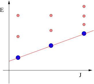
Figure 1: The annulon trajectory obtained as a plot of the lowest mass annulon for a given charge.

Some remarks are in order. The expression (6.12) is the same for all annulons discussed in this and in previous papers and is therefore universal. There is an implicit assumption that $J$ and $E$ are very large quantum numbers so that the semiclassical analysis can be trusted. The factor $\alpha_{0}$ is determined by the zero point energy discussed in the previous section. As the excited state energy, it is a function of $J$ in the ratio $J/\lambda$. Since both $J$ and $\lambda$ are parametrically large, it gives a subleading correction (in $J$) to the linear relation (6.12). Note that for higher values of the charge $J$, the distance between excited states in the same tower decreases.

These annulon trajectories are different from the Regge trajectories where one obtains a straight line in a plot of spin versus mass square, $E^{2}$. Interestingly, the appearance of $E$ rather than $E^{2}$ took place in a recent analysis of Regge trajectories in the context of the gauge/gravity correspondence [54].

7 Non-supersymmetric deformations of the resolved conifold

In section 3, we analyzed the IIA background corresponding to a resolved conifold metric with RR two-form flux over the blown up $S^{2}$. This is dual to ${\cal N}=1$ SYM and is obtained by reduction of an eleven dimensional background which contains a $G_{2}$ holonomy metric in the $D_{7}$ family [9, 10].

In this section, we look for non-supersymmetric deformations of the above background. In particular, we would like to find seven dimensional metrics whose asymptotics are similar to the supersymmetric ones. The ansatz is exactly the same as Eq.(3.1), namely

$$ds^{2} =dr^{2}+a(r)^{2}\left[(\Sigma_{1}+g(r)\sigma_{1})^{2}+(\Sigma_{2}+g(r)\sigma_{2})^{2}\right]$$

$$+c(r)^{2}(\Sigma_{3}+g_{3}(r)\sigma_{3})^{2}+b(r)^{2}\left[\sigma_{1}^{2}+\sigma_{2}^{2}\right]+f(r)^{2}\sigma_{3}^{2}\,.$$ (7.1)

The results are as follows. We found a family of regular non-supersymmetric solutions with $g(r)\equiv 0$ but otherwise essentially the same small $r$ behavior as the supersymmetric ones.

As in the supersymmetric case, upon reduction to Type IIA, the dilaton is still finite everywhere. However, the large $r$ asymptotic properties differ dramatically from the supersymmetric case. In particular, there are two stabilized one-cycles instead of one. The IIA metric in string frame reads

$$e^{-2\Phi/3}ds_{10}^{2}=dx_{1,3}^{2}+\ell^{2}\bigl{[}dr^{2}+a(r)^{2}(d\bar{\theta}^{2}+\sin^{2}\bar{\theta}d\bar{\phi}^{2})+b(r)^{2}(d\theta^{2}+\sin^{2}\theta d\phi^{2})+$$

$$+\frac{f^{2}c^{2}}{f(r)^{2}+(1+g_{3}(r))^{2}c(r)^{2}}(d\psi_{2}-\cos\theta d\phi+\cos\bar{\theta}d\bar{\phi})^{2}\bigr{]},$$

and the radius of the circle parametrized by $\psi_{2}$ has a finite limit as $r\to\infty$. The matter fields are given as before by

$$A_{1}=\ell N\bigg{[}\frac{f(r)^{2}-(1-g_{3}(r)^{2})c^{2}}{f(r)^{2}+(1+g_{3}(r))^{2}c(r)^{2}}(-d\psi_{2}+\cos\theta d\phi-\cos\bar{\theta}d\bar{\phi})+$$

$$\qquad\qquad+\cos\theta d\phi+\cos\bar{\theta}d\bar{\phi}\bigg{]},$$

$$4N^{2}e^{4\Phi/3}=f(r)^{2}+c(r)^{2}(1+g_{3}(r))^{2}.$$ (7.2)

Ricci flatness implies that the functions $\{a(r),b(r),c(r),f(r),g(r),g_{3}(r)\}$ satisfy a coupled system of six second order nonlinear differential equations supplemented by a constraint. The precise form of these equations can be found in appendix E. From consistency with the equations of motion and the requirement that the solution be regular at $r=0$, one can derive the following boundary conditions

$$b =R_{0}-\left(\frac{q_{0}^{2}-2}{16R_{0}}\right)r^{2}+{\cal O}(r^{4})\,,$$

$$f =q_{0}R_{0}+\frac{q_{0}^{3}}{16R_{0}}r^{2}+{\cal O}(r^{4})\,,$$

$$a =\frac{1}{2}r+\left(\frac{q_{0}^{2}-4R_{0}^{2}}{192R_{0}^{2}}+\frac{c_{0}}{2}\right)r^{3}+{\cal O}(r^{5})\,,$$

$$c =-\frac{1}{2}r+c_{0}r^{3}+{\cal O}(r^{5})\,,$$

$$g =\frac{q_{0}}{2}+\alpha+\left[\frac{(q_{0}+2\alpha)\left((q_{0}^{2}+\beta)^{2}+q_{0}^{2}(\alpha^{2}+\alpha q_{0}-1)\right)}{24q_{0}^{2}R_{0}^{2}}\right]r^{2}+{\cal O}(r^{4})\,,$$

$$g_{3} =\left(\frac{q_{0}^{2}}{2}-1+\beta\right)+\left[\frac{(4\alpha^{2}+4\alpha q_{0})(q_{0}^{2}+\beta)+q_{0}^{2}(2q_{0}^{2}-2+3\beta)}{24R_{0}^{2}}\right]r^{2}+{\cal O}(r^{4})\,.$$ (7.3)

The supersymmetric solutions correspond to

$$c_{0}=-\frac{5q_{0}^{2}-8}{288R_{0}^{2}}\,,\quad\alpha=0\,,\quad\beta=0\,.$$ (7.4)

In particular, these boundary conditions imply that $g(r)=-\frac{af}{2bc},\,g_{3}(r)=2g(r)^{2}-1$ for any value of $r$.

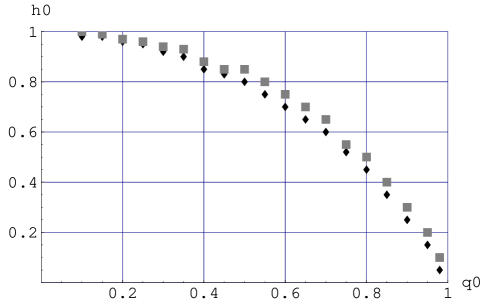
Figure 2: Every value of $h_{0}$ below a diamond gives a regular solution, whereas every value above a box leads to a singular one. Also, recall that the full range is symmetric under $h_{0}\to-h_{0}$.

The only non-singular non-supersymmetric solutions we were able to find correspond to setting $\alpha=-\frac{q_{0}}{2}$. Note that this is not a small deviation from the supersymmetric case. In fact, by virtue of the equations of motion, $\alpha=-\frac{q_{0}}{2}$ implies that $g(r)\equiv 0$. The value of $c_{0}$ is still the same as in the supersymmetric case. Thus, besides the usual parameters $q_{0}$ and $R_{0}$, these solutions depend on the value of $\beta$. Numerical analysis shows that there is actually only a finite range of values of $h_{0}\equiv\frac{q_{0}^{2}}{2}-1+\beta$ such that the solution is regular and finite everywhere ( see Fig. 2 ). If $h_{0}$ lies outside this range, the solution develops a singularity at a finite value of $r$. Note also that, since the equations of motion are symmetric under $g_{3}(r)\to-g_{3}(r)$, which is true only if $g(r)\equiv 0$, the range of allowed values for $h_{0}$ is symmetric under $h_{0}\to-h_{0}$.

These solutions are markedly different from the supersymmetric ones. First of all, both $f(r)$ and $c(r)$ approach a constant value in the limit $r\to\infty$. As a consequence, the Type IIA metric is not asymptotically conical as in the supersymmetric case. In fact, the fibered $S^{1}$ parametrized by $\psi_{2}$ has actually a finite radius at infinity. As $r\to\infty$, a generic solution has the following behavior

$$a(r) =\frac{r+r_{\infty}}{\sqrt{3}}+\frac{3\sqrt{3}\left(\,q_{2}^{2}(1+2g_{\infty}^{2})+2\,\right)R_{2}^{2}}{8(\,r+r_{\infty})}-\frac{c_{3}+q_{2}f_{3}}{2\sqrt{3}q_{2}R_{2}(\,r+r_{\infty})^{2}}+...$$

$$b(r) =\frac{r+r_{\infty}}{\sqrt{3}}+\frac{3\sqrt{3}\left(\,q_{2}^{2}(2+g_{\infty}^{2})+1\,\right)R_{2}^{2}}{8(\,r+r_{\infty})}-\frac{c_{3}+q_{2}f_{3}}{2\sqrt{3}q_{2}R_{2}(\,r+r_{\infty})^{2}}+...$$

$$c(r) =q_{2}R_{2}-\frac{9q_{2}^{3}R_{2}^{3}(1+g_{\infty}^{2})}{4(\,r+r_{\infty})^{2}}+\frac{c_{3}}{(\,r+r_{\infty})^{3}}+...$$

$$f(r) =R_{2}-\frac{9R_{2}^{3}}{4(\,r+r_{\infty})^{2}}+\frac{f_{3}}{(\,r+r_{\infty})^{3}}+...$$

$$g_{3}(r) =g_{\infty}-\frac{9R_{2}^{2}g_{\infty}}{2(\,r+r_{\infty})^{2}}+\frac{h_{\infty}}{(\,r+r_{\infty})^{3}}+...$$ (7.5)

where the seven parameters involved, $\{q_{2},R_{2},c_{3},f_{3},g_{\infty},h_{\infty},r_{\infty}\}$, will depend on the three IR parameters $\{q_{0},R_{0},h_{0}\}$. The dilaton is still finite everywhere, just like in the supersymmetric case.

The RR two-form flux through the non-collapsing two-sphere at infinity parametrized by $\theta$ and $\phi$ is not equal to $1$ as in the supersymmetric case. This is because the first term in the RR gauge field (7) proportional to $\sigma_{3}-\Sigma_{3}$, namely $A(r)\equiv\frac{f^{2}-(1-g_{3})^{2}c^{2}}{f^{2}+(1+g_{3})^{2}c^{2}}$, does not vanish for $r\to\infty$ as in the supersymmetric case. Actually, in the limit $r\to\infty$, it always goes to a negative constant, which in general is not even an integer. However, the flux through the two-sphere defined by $\psi_{2}=0,\theta=\bar{\theta},\phi=\bar{\phi}$ is always equal to $2N$, independently of the limit of $A(r)$. This holds for supersymmetric solutions too. Note that this sphere does not collapse either, since its area is proportional to $b(r)^{2}+a(r)^{2}$.

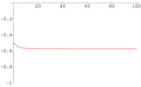
Figure 5: Plot of $g_{3}$.

To create a more detailed and intuitive picture we show a generic solution corresponding to $\{R_{0}=1,q_{0}=\frac{1}{2},h_{0}=-\frac{1}{2}\}$ in figures 3-7. Fig. 7 shows that the term $A(r)\equiv\frac{f^{2}-(1-g_{3})^{2}c^{2}}{f^{2}+(1+g_{3})^{2}c^{2}}$ is not asymptotic to an integer constant. Setting $h_{0}=-0.395$ instead, we find a solution such that $\lim_{r\to\infty}A(r)=-2$ ( Fig. 8 ). The asymptotic values of $e^{\Phi}$ and $c(r)$ are different in the two cases ( Figs. 9,  10) , whereas the profiles of $a(r),b(r)$ and $f(r)$ are virtually the same. In Figs. 11-16, we compare the supersymmetric solution for $\{R_{0}=1,q_{0}=\frac{1}{2}\}$ and the non-supersymmetric one corresponding to $\{R_{0}=1,q_{0}=\frac{1}{2},h_{0}=-0.395\}$.

Interestingly, the Penrose limit, with the particular geodesic of section 3, of these non-supersymmetric solutions is exactly the same as the Penrose limit of the supersymmetric ones with the same value of $q_{0}$. This enhancement of supersymmetry for the Penrose limit of certain supergravity backgrounds was first noticed in [50, 51] for the case of $AdS_{5}\times T^{1,1}$ which has the same Penrose limit as $AdS_{5}\times S^{5}$. Basically, the Penrose limit of a general solution whose behavior close to $r=0$ is given by Eqs.(7.3) is exactly the same as the supersymmetric one. The metric reads

$$ds^{2} =-4dx^{+}dx^{-}-m_{0}^{2}\bigg{[}v^{2}+\frac{(2q_{0}^{2}-4(1+g_{0}^{2}))}{16}y^{a}y_{a}\bigg{]}(dx^{+})^{2}+dx^{i}dx_{i}+dy^{a}dy_{a}+dv^{2}$$

$$+m_{0}g_{0}dx^{+}(y_{1}dy_{3}-y_{3}dy_{1}+y_{2}dy_{4}-y_{4}dy_{2})\,,$$ (7.6)

where $g_{0}\equiv\frac{q_{0}}{2}+\alpha$. For the family of non-supersymmetric solutions that we found, one has $g_{0}\equiv 0$. In general, with the following coordinate transformation

$$u=e^{i\frac{m_{0}g_{0}x^{+}}{2}}(y_{1}+iy_{3}),\qquad z=e^{i\frac{m_{0}g_{0}x^{+}}{2}}(y_{2}+iy_{4}),$$

we retrieve Eq.(3.15). This property of supersymmetry enhancement in the Penrose limit gives further evidence that the nonsupersymmetric deformation is different from the other soft susy breaking achieved by means of a gaugino bilinear. This kind of supersymmetry breaking seems to be similar to the breaking between the ${\cal N}=4$ SYM corresponding to string theory on $AdS_{5}\times S^{5}$ and the ${\cal N}=1$ SCFT dual to $AdS_{5}\times T^{1,1}$.

In summary, for given values of $q_{0}$ and $R_{0}$, there is a one-parameter family of non-supersymmetric solutions whose flux through the non-collapsing two-sphere defined by $\psi_{2}=0,\theta=\bar{\theta},\phi=\bar{\phi}$ is equal to $2N$, like in the supersymmetric case. The asymptotic behavior of these solutions differs from the supersymmetric case in that the IIA metric is not conical for large $r$ but has a finite radius circle instead.

8 Conclusions

Let us summarize our main results and comment on possible extensions or the work presented here.

First we should emphasize, once again, that this paper deals with supergravity duals to confining gauge theories. For the supergravity approximation to be well defined we need the curvature of the metric to be small in string units. Small curvature implies that the field theory dual is not simply that of the ‘pure’ gauge theory. Instead, the dual necessarily includes adjoint massive fields (KK modes). These inconvenient ‘impurities’ plague all the known gravity duals to confining gauge theories.

As mentioned in the introduction, this work focuses on the “hadrons” composed out of a large number of the adjoint massive fields referred above. These hadrons are shown to be ubiquitous in duals to confining theories, and some common features are investigated in this paper.

To address some of the dynamical features of these hadrons we used a Penrose limit that was motivated in [4]. Basically, we used a null geodesic localized in the region of small values of the radial coordinate. By taking this Penrose limit we found a parallel plane wave associated to a sector of the confining dual. Then, quantizing the Type II superstring on the pp-wave we analyzed several features common to all these confining backgrounds. Among these features we discussed: a mass formula for the ground state and its excitations, the composition of the hadrons in terms of KK modes, the existence of ‘universal’ sectors, zero point energies, and a experimental signature for the annulon trajectories.

It is worth highlighting that we considered backgrounds dual to minimally supersymmetric field theories, that is, with four supercharges in four dimensions and two supercharges in three dimensions. We also considered backgrounds where supersymmetry is explicitly broken. The breaking procedure is ‘soft’ in the 3-d model of section 4, in the sense that it is based on the de-tuning of one parameter; this is not the case for the 4-d model of section 7. The general structure of our hadrons does not seem to be too sensitive to the breaking. In fact, it also coincides with the same general type studied before. The persistence of this structure for backgrounds in IIB, IIA, dual to confining gauge theories in four and three dimensions, encourages us to view this fact as a sign of the universality of the hadrons.

There are, of course, some differences in the several cases that we considered. In the case of duals to confining three dimensional gauge theories (Type IIB or IIA cases), everything seems to work nicely. In the M-theory or IIA set up dual to four dimensional ${\cal N}=1$ SYM + KK modes there are issues with the lower modes. These problems do not seem to indicate an instability in the free strings case, but the introduction of interactions could render the plane wave geometry unstable. This is obviously one of the features that deserve further study.

Other than the universality of annulons we have established the existence of a Hagedorn density of states for the strings quantized in these backgrounds. This is the expected behavior for hadronic matter. On the more technical side of this question, we have included a discussion (hopefully fairly clear) on the issue of regularizations of the zero point energies of the backgrounds under study; this can be find in appendix D.

In section 7, we have numerically constructed new solutions that are non supersymmetric versions of $G_{2}$ holonomy manifolds in M-theory (or Type IIA with fluxes on the resolved conifold). These solutions are ALC, thus having a consistent IIA interpretation as branes wrapping cycles in a non-supersymmetric fashion. It would be of interest to study properties of this solutions in relation to their argued field theory dual. The stability of these new solutions is also a point to be studied.

What are the future directions of research that this investigation opens? In view of their universality, these hadrons deserve more study. Indeed, the present paper and its predecessors seem to be the only quantitative prediction for the KK modes. The scattering properties, a detailed study of the annulon trajectories discussed in section 6.3, seem to be natural directions to concentrate further efforts.

Appendix A Parametrization of $\mathbb{R}^{4}$

The left-invariant one forms of $SU(2)$ are defined as

$$\sigma_{1}+i\sigma_{2}=e^{-i\psi}(d\theta+i\sin\theta d\phi),\qquad\sigma_{3}=d\psi+\cos\theta d\phi.$$ (A.1)

Note that they satisfy $d\sigma_{1}=-\sigma_{2}\wedge\sigma_{3}$.

The change of coordinates on $\mathbb{R}^{4}$ used in the main text is

$$y_{1}=r\sin{\theta\over 2}\sin{{\psi-\phi}\over 2},\quad y_{2}=r\sin{\theta\over 2}\cos{{\psi-\phi}\over 2},$$

$$y_{3}=r\cos{\theta\over 2}\cos{{\psi+\phi}\over 2},\quad y_{4}=r\cos{\theta\over 2}\sin{{\psi+\phi}\over 2}.$$ (A.2)

Note that with this definitions the metric in $\mathbb{R}^{4}$ is

$$ds^{2}=dr^{2}+{r^{2}\over 4}(\sigma_{1}^{2}+\sigma_{2}^{2}+\sigma_{3}^{2})=dy^{a}dy_{a},$$ (A.3)

with $a=1,2,3,4$.

Appendix B Fermionic equations of motion

In the generic Type IIA case the equations of motion of the world-sheet fermions read (see for example [55] and related papers)

$$(\partial_{\tau}+\partial_{\sigma})\theta^{1} = {\alpha^{\prime}p^{+}\over{4}}e^{\Phi}F_{+i}\Gamma^{i}\theta^{2}+{\alpha^{\prime}p^{+}\over{8}}H_{+ij}\Gamma^{ij}\theta^{1}-{\alpha^{\prime}p^{+}\over{24}}e^{\Phi}F_{+ijk}\Gamma^{ijk}\theta^{2},$$

$$(\partial_{\tau}-\partial_{\sigma})\theta^{2} = -{\alpha^{\prime}p^{+}\over{4}}e^{\Phi}F_{+i}\Gamma^{i}\theta^{1}-{\alpha^{\prime}p^{+}\over{8}}H_{+ij}\Gamma^{ij}\theta^{2}-{\alpha^{\prime}p^{+}\over{24}}e^{\Phi}F_{+ijk}\Gamma^{ijk}\theta^{1}.$$ (B.1)

The relevant IIB equations are [4]

$$(\partial_{\tau}+\partial_{\sigma})\theta^{1} = -{\alpha^{\prime}p^{+}\over{8}}e^{\Phi}F_{+ij}\Gamma^{ij}\theta^{2}-{\alpha^{\prime}p^{+}\over{8}}H_{+ij}\Gamma^{ij}\theta^{1},$$

$$(\partial_{\tau}-\partial_{\sigma})\theta^{2} = -{\alpha^{\prime}p^{+}\over{8}}e^{\Phi}F_{+ij}\Gamma^{ij}\theta^{1}+{\alpha^{\prime}p^{+}\over{8}}H_{+ij}\Gamma^{ij}\theta^{2}.$$ (B.2)

Appendix C The BPST Instanton

In this appendix we present the explicit form of the one-instanton field that we use in the main text. We present the coordinate change of variables that takes the explicit solution of [49] into the one used in the main text. The metric on $S^{4}$ and the correspondent one-instanton are [49]:

$$ds^{2} = {1\over(1+r^{2}/a^{2})^{2}}\bigg{[}dr^{2}+{1\over 4}r^{2}(\sigma_{1}^{2}+\sigma_{2}^{2}+\sigma_{3}^{2})\bigg{]},$$

$$A^{1} = -\sigma_{1}\,{(r/a)^{2}\over 1+r^{2}/a^{2}},\qquad{\rm cyclic}.$$ (C.1)

Taking

$$\sin\psi={2r/a\over 1+r^{2}/a^{2}},$$ (C.2)

we find

$$ds^{2} = {a^{2}\over 4}\bigg{[}d\psi^{2}+{1\over 4}\sin^{2}\psi(\sigma_{1}^{2}+\sigma_{2}^{2}+\sigma_{3}^{2})\bigg{]},$$

$$A^{1} = -{1\over 2}(1-\cos\psi)\,\,\sigma_{1},\qquad{\rm cyclic}.$$ (C.3)

These are the expressions used in the main text. The radius of $S^{4}$ or alternatively the size of the instanton is set to $a=2$.

The corresponding field strength is given by $J^{i}=dA^{i}+\frac{1}{2}\epsilon_{ijk}A^{j}\wedge A^{k}$

$$J^{1}=-{1\over 2}\sin\psi d\psi\wedge\sigma_{1}-{1\over 4}\sin^{2}\psi\,\,\sigma_{2}\wedge\sigma_{3},\qquad{\rm cyclic}.$$ (C.4)

Appendix D Zero point energy

In this appendix we will briefly discuss two of the procedures most commonly encountered in the literature to deal with the zero point energy. We attempt to describe their similarities and differences. We hope this appendix clarifies why our preference falls on the one used in the main text.

The Penrose limits we took in this paper always resulted in plane-waves preserving only 16 supersymmetries. These are the so-called “kinematical” supercharges, which give no linearly realized supersymmetry on the worldsheet [56]. This is evident by examining the various string spectra we found: worldsheet bosons and fermions have generically different worldsheet masses. Thus the zero point energy $E_{0}(m)$ is not trivial. In particular two aspects of it are relevant: its negative sign and its actual behavior as a function of $m$. As we will show, the first is independent on the way in which $E_{0}$ is evaluated, while the latter is strongly dependent on it.

The general way in which we wrote $E_{0}$ is in terms of an expression like

$$S(m)={1\over 2}\sum_{n=-\infty}^{\infty}[\sum_{i=1}^{8}\sqrt{n^{2}+b_{i}^{2}m^{2}}-\sum_{j=1}^{8}\sqrt{n^{2}+f_{i}^{2}m^{2}}],$$ (D.1)

where $b_{i}$ and $f_{i}$ parameterize the bosonic and fermionic masses respectively. The supergravity equations of motion crucially imply $\sum_{i}b_{i}^{2}=\sum_{j}f_{j}^{2}$. Under this condition it is easy to show that the above series is convergent, has definite sign (negative in all the models we examined, apart from the by now problematic IIA resolved conifold one) and is linear in $m^{2}$ in the large $m$ limit. We will return on these points in a moment. There is in fact a formal subtlety here we want to alert the reader about. Since the single bosonic and fermionic contributions of the whole expression above are divergent, we cannot trivially say that the expression in (D.1) is equal to

$$S_{B}(m)-S_{F}(m)={1\over 2}\sum_{n=-\infty}^{\infty}\sum_{i=1}^{8}\sqrt{n^{2}+b_{i}^{2}m^{2}}-{1\over 2}\sum_{n=-\infty}^{\infty}\sum_{j=1}^{8}\sqrt{n^{2}+f_{j}^{2}m^{2}}.$$ (D.2)

If we write $E_{0}$ in these terms, we have to find a regularization prescription to carefully deal with the divergent terms

$${1\over 2}\sum_{n=-\infty}^{\infty}\sqrt{n^{2}+m^{2}}.$$ (D.3)

One way is to regularize these is by considering

$$\sum\limits_{n\in\mathbb{Z}}\sqrt{n^{2}+m^{2}}\longrightarrow\sum\limits_{n\in\mathbb{Z}}(n^{2}+m^{2})^{-s}.$$ (D.4)

Let us thus evaluate this expression

$${1\over 2}\sum\limits_{n\in\mathbb{Z}}(n^{2}+m^{2})^{-s}=$$

$$\qquad={1\over 2}\sum\limits_{n\in\mathbb{Z}}{1\over\Gamma(s)}\int\limits_{0}^{\infty}dtt^{s-1}e^{-t(m^{2}+n^{2})}$$

$$\qquad={1\over 2}\sum\limits_{p\in\mathbb{Z}}{\pi^{1/2}\over\Gamma(s)}\int\limits_{0}^{\infty}dtt^{s-3/2}e^{-tm^{2}-\pi^{2}p^{2}/t}$$

$$\qquad={1\over 2}{\pi^{1/2}\over\Gamma(s)}\left(2\sum\limits_{p=1}^{\infty}\int\limits_{0}^{\infty}dtt^{s-3/2}e^{-tm^{2}-\pi^{2}p^{2}/t}+\int\limits_{0}^{\infty}dtt^{s-3/2}e^{-tm^{2}}\right)$$ (D.5)

$$\qquad={1\over 2}{\pi^{1/2}\over\Gamma(s)}2\sum\limits_{p=1}^{\infty}2\left({\pi^{2}p^{2}\over m^{2}}\right)^{s/2-1/4}K_{s-1/2}(2\pi\;p\;m)+{1\over 2}{\pi^{-s}\over\Gamma(s)}\int\limits_{0}^{\infty}dt\;t^{s-3/2}e^{-tm^{2}}$$

$$\qquad=2{\pi^{s}(m^{2})^{-s/2+1/4}\over\Gamma(s)}\sum\limits_{p=1}^{\infty}{1\over p^{1/2-s}}K_{s-1/2}(2\pi\;p\;m)+{1\over 2}{\pi^{1/2}\over\Gamma(s)}(m^{2})^{-s+1/2}\;\Gamma(s-1/2).$$

In step 1 we used [57]

$$\int\limits_{0}^{\infty}dt\;t^{\nu-1}e^{-\mu t}=\mu^{-\nu}\Gamma(\nu),$$ (D.6)

with $\mu=m^{2}+n^{2}$ and $\nu=s$. Note that the $\Gamma$ function provides a natural analytical continuation for $\nu=-1/2$. Step 2 uses the Poisson resummation formula:

$$\sum\limits_{n\in Z}e^{-t\;n^{2}}=\left({\pi\over t}\right)^{1/2}\sum\limits_{p\in Z}e^{-\pi^{2}p^{2}/t}.$$ (D.7)

In step 4 we used [57]

$$\int\limits_{0}^{\infty}dtt^{\nu-1}e^{-t\gamma-\beta/t}=2\left({\beta\over\gamma}\right)^{\nu/2}K_{\nu}(2\sqrt{\gamma\beta}).$$ (D.8)

The above expression (D) is divergent in the limit $s\to-1/2$.

A prescription commonly found in the literature consists in defining (D.3) by assigning it the finite value corresponding to ignoring the second term in the last expression in (D). Basically this defines a “renormalized” (Casimir energy like) version of (D.3) to be the term containing the sum of Bessel functions. If we apply this prescription to each term in (D.2) and then sum up, we find that the whole zero point energy is given by a sum over Bessel functions only.

In the main body of the paper we followed instead a different “regularization” prescription as suggested in [41]. We did not take the $s\to-1/2$ limit for each individual degree of freedom. Instead we first added the contribution of bosons and fermions as in (D.1) and only at the end we sent $s\to-1/2$. These two prescriptions give two slightly different results.

Renormalizing individual degrees of freedom is justified and necessary in the bosonic string cases in order to deal with infinities as we do in ordinary bosonic field theories. A deeper reason for this is provided by the fact that in a bosonic theory the zero point or Casimir energy is an observable and thus we renormalize it to obtain a finite result. In the supersymmetric cases the natural objects to look at are the boson-fermion constituents and the observable quantity is the one obtained by summing the contributions of all degrees of freedom as in (D.1). In a sense this choice amounts on choosing the same regulator (say, the same cutoff) for all the degrees of freedom, and this is physically sensible. This way no renormalization prescription is required: we only need a calculation tool to evaluate a convergent quantity.

In our case, we can thus decide to evaluate the expression in (D.1) by using the $s$-regularization as above, i.e. taking the $s\to-1/2$ limit of $S(m,s)$. Due to the condition $\sum_{i}b_{i}^{2}=\sum_{j}f_{j}^{2}$, it follows that the leading divergence coming from $\Gamma(-1+\epsilon)$ with $\epsilon\to 0$ in (D) always cancels in $S$. The final result is

$$S(m) = \sum_{i=1}^{8}[2{(b_{i}m)\over\pi^{1/2}\Gamma(-1/2)}\sum\limits_{p=1}^{\infty}{1\over p}K_{-1}(2\pi\;p\;b_{i}m)]+$$ (D.9)

$$- \sum_{j=1}^{8}[2{(f_{j}m)\over\pi^{1/2}\Gamma(-1/2)}\sum\limits_{p=1}^{\infty}{1\over p}K_{-1}(2\pi\;p\;f_{j}m)]+$$

$$- {m^{2}\over 2}[\sum_{i=1}^{8}b_{i}^{2}\log b_{i}^{2}-\sum_{j=1}^{8}f_{j}^{2}\log f_{j}^{2}],$$

the last line tracing the difference between our prescription and the Casimir-like one. Let us notice that in the case where supersymmetry is linearly realized and so bosons and fermions are arranged in multiplets sharing the same masses, this last term is zero, and so the two prescriptions give the same result. In the general case the difference manifests itself in the large $m$ limit.

By referring to the notations used in the paper the zero point energy reads $E_{0}(m)=(m_{0}/m)S(m)$ . In the small $m$ limit only the zero-modes are leading order and $E_{0}(m)\to m_{0}(\sum_{i}|b_{i}|-\sum_{j}|f_{j}|)$: this can be found by using both prescriptions. As a remark we noticed in the paper that for all the confining models we examined this quantity is negative.

In the large $m$ limit, if we Casimir-renormalize each term in the sum by associating it with the term containing only the sum of Bessel functions, we get zero for the zero point energy. This is because the Bessel function vanishes exponentially for large values of the argument. Our prescription instead add to the Bessel terms the last line in (D.9), giving to $E_{0}$ a linear behavior in $m$, for large $m$. In the models we examined this reads as $E_{0}\approx-m_{0}A^{2}m$, where $A^{2}$ is a model-dependent constant.

As a remark, disconnected from the choice of the evaluation prescription for the zero point energy, and related to the models we examine in the main body of the paper, we should ask which kind of consequences the negativity of the superstring zero point energy $E_{0}(m)$ should have at string level.

In the limit $m<<1$ (this is usually referred to as the “supergravity limit” as the leading order contribution to the string motion comes from the zero-modes) we can study the consequences (or the meaning) of the negativity of $E_{0}$ by referring to supergravity. So, the question is: does the negative value of the zero point energy correspond to some (classical) instability of the backgrounds here considered? In was shown in [41] that in all the cases in which $E_{0}$ stays finite in the supergravity limit, no instability can be read from the supergravity perspective, no matter the sign of $E_{0}$. The situation is problematic only when $E_{0}$ goes to minus infinity for $m\to 0$ (just as in the Type 0B case considered in [42]) where a tachyonic instability appears.

Appendix E Ricci flatness

Imposing that the seven-dimensional metric (7.1) is Ricci flat, we find the following system of equations

$$a^{\prime\prime}= \frac{1}{20a^{3}b^{4}c^{2}f^{2}}[-9b^{4}c^{4}f^{2}-8a^{2}b^{2}c^{2}f^{2}(c^{2}g^{2}+2b^{2}(a^{\prime}{}^{2}-1))$$

$$- 12a^{3}b^{3}cfa^{\prime}(bfc^{\prime}+c(2fb^{\prime}+bf^{\prime}))$$

$$+ 4a^{6}b^{2}(3f^{2}g^{2}+c^{2}(3g^{2}(1+g_{3})^{2}+2f^{2}g^{\prime}{}^{2}))$$

$$+ a^{4}c\,(cf^{2}(f^{2}+c^{2}(g^{2}+g_{3})^{2})-4b^{2}cf^{2}(1+g^{2}-b^{\prime}{}^{2})$$

$$+ 8b^{3}fb^{\prime}(fc^{\prime}+cf^{\prime})+b^{4}(4fc^{\prime}f^{\prime}-c^{3}g_{3}^{\prime}{}^{2}))]$$ (E.1)

$$b^{\prime\prime}= \frac{1}{20a^{4}b^{3}c^{2}f^{2}}[b^{4}c^{4}f^{2}+4a^{2}b^{2}c^{2}f^{2}(-2c^{2}g^{2}+b^{2}(a^{\prime}{}^{2}-1))$$

$$+ 8a^{3}b^{3}cfa^{\prime}(bfc^{\prime}+c(-3fb^{\prime}+bf^{\prime}))$$

$$- 4a^{6}b^{2}(2f^{2}g^{2}+c^{2}(2g^{2}(1+g_{3})^{2}+3f^{2}g^{\prime}{}^{2}))$$

$$- a^{4}c\,(9cf^{2}(f^{2}+c^{2}(g^{2}+g_{3})^{2})-16b^{2}cf^{2}(1+g^{2}-b^{\prime}{}^{2})$$

$$+ 12b^{3}fb^{\prime}(fc^{\prime}+cf^{\prime})+b^{4}(-4fc^{\prime}f^{\prime}+c^{3}g_{3}^{\prime}{}^{2}))]$$ (E.2)

$$c^{\prime\prime}= \frac{1}{20a^{4}b^{4}cf^{2}}[11b^{4}c^{4}f^{2}+2a^{2}b^{2}c^{2}f^{2}(11c^{2}g^{2}+2b^{2}(a^{\prime}{}^{2}-1))$$

$$+ 8a^{3}b^{3}cfa^{\prime}(-4bfc^{\prime}+c(2fb^{\prime}+bf^{\prime}))$$

$$+ 2a^{6}b^{2}(-9f^{2}g^{2}+c^{2}(g^{2}(1+g_{3})^{2}-f^{2}g^{\prime}{}^{2}))$$

$$+ a^{4}c\,(cf^{2}(f^{2}+11c^{2}(g^{2}+g_{3})^{2})-4b^{2}cf^{2}(1+g^{2}-b^{\prime}{}^{2})$$

$$+ 8b^{3}fb^{\prime}(-4fc^{\prime}+cf^{\prime})+b^{4}(-16fc^{\prime}f^{\prime}+9c^{3}g_{3}^{\prime}{}^{2}))]$$ (E.3)

$$f^{\prime\prime}= \frac{1}{20a^{4}b^{4}c^{2}f}[b^{4}c^{4}f^{2}+2a^{2}b^{2}c^{2}f^{2}(c^{2}g^{2}+2b^{2}(a^{\prime}{}^{2}-1))$$

$$+ 8a^{3}b^{3}cfa^{\prime}(bfc^{\prime}+2c(fb^{\prime}-2bf^{\prime}))$$

$$- 2a^{6}b^{2}(-f^{2}g^{2}+c^{2}(9g^{2}(1+g_{3})^{2}+f^{2}g^{\prime}{}^{2}))$$

$$+ a^{4}c\,(cf^{2}(11f^{2}+c^{2}(g^{2}+g_{3})^{2})-4b^{2}cf^{2}(1+g^{2}-b^{\prime}{}^{2})$$

$$+ 8b^{3}fb^{\prime}(fc^{\prime}-4cf^{\prime})-b^{4}(16fc^{\prime}f^{\prime}+11c^{3}g_{3}^{\prime}{}^{2}))]$$ (E.4)

$$g^{\prime\prime}= \frac{c^{2}g}{a^{4}}+\frac{g(-2b^{2}+c^{2}(g^{2}+g_{3}))}{a^{2}b^{2}}+\frac{f^{2}g+c^{2}g(1+g_{3})^{2}}{c^{2}f^{2}}$$

$$- \left(\frac{4a^{\prime}}{a}+\frac{c^{\prime}}{c}+\frac{f^{\prime}}{f}\right)g^{\prime}$$ (E.5)

$$g_{3}^{\prime\prime}= \frac{2a^{2}g^{2}(1+g_{3})}{b^{2}c^{2}}+\frac{f^{2}(g^{2}+g_{3})}{b^{4}}$$

$$- \left(\frac{2a^{\prime}}{a}+\frac{2b^{\prime}}{b}+\frac{3c^{\prime}}{c}-\frac{f^{\prime}}{f}\right)g^{\prime}_{3}$$ (E.6)

together with the constraint

$$-\frac{1}{2a^{2}b^{2}cf} [b^{4}c^{4}f^{2}+2a^{2}b^{2}c^{2}f^{2}(c^{2}g^{2}+2b^{2}(a^{\prime}{}^{2}-1))$$

$$+ 8a^{3}b^{3}cfa^{\prime}(bfc^{\prime}+c(2fb^{\prime}+bf^{\prime}))$$

$$+ 2a^{6}b^{2}(f^{2}g^{2}+c^{2}(g^{2}(1+g_{3})^{2}-f^{2}g^{\prime}{}^{2}))$$

$$+ a^{4}c\,(cf^{2}(f^{2}+c^{2}(g^{2}+g_{3})^{2})-4b^{2}cf^{2}(1+g^{2}-b^{\prime}{}^{2})$$

$$+ 8b^{3}fb^{\prime}(fc^{\prime}+cf^{\prime})+b^{4}(4fc^{\prime}f^{\prime}-c^{3}g_{3}^{\prime}{}^{2}))]=0\,.$$ (E.7)

The system is invariant under translations, $r\to r+const$.

Furthermore, if $\{a(r),b(r),c(r),f(r),g(r),g_{3}(r)\}$ is a solution of the equations of motion then $\{\lambda^{-1}a(\lambda r),\lambda^{-1}b(\lambda r),\lambda^{-1}c(\lambda r),\lambda^{-1}f(\lambda r),g(\lambda r),g_{3}(\lambda r)\}$ is a solution too $(\lambda\neq 0)$. There is also a symmetry under $g(r)\to-g(r)$. Finally, in the case $g(r)\equiv 0$, there is an extra symmetry under $g_{3}(r)\to-g_{3}(r)$.

Figure 3: The functions $a$ (dashed line) and $b$ (continuous line).

Figure 4: Plot of $-c$ (continuous line) and $f$ (dashed line).

Figure 6: Plot of $e^{\Phi}$.

Figure 7: Plot of $A(r)\equiv\frac{f^{2}-(1-g_{3})^{2}c^{2}}{f^{2}+(1+g_{3})^{2}c^{2}}$.

Figure 8: Plot of $A(r)$ for $\{R_{0}=1,q_{0}=\frac{1}{2},h_{0}=-0.395\}$.

Figure 9: Plot of $e^{\Phi}$ for $\{R_{0}=1,q_{0}=\frac{1}{2},h_{0}=-0.5\}$ (continuous line) and $\{R_{0}=1,q_{0}=\frac{1}{2},h_{0}=-0.395\}$ (dashed line).

Figure 10: Plot of $-c$ for $\{R_{0}=1,q_{0}=\frac{1}{2},h_{0}=-0.5\}$ (continuous line) and $\{R_{0}=1,q_{0}=\frac{1}{2},h_{0}=-0.395\}$ (dashed line).

Figure 11: The functions $a$ and $b$ for the supersymmetric (dashed line) and non-supersymmetric solution (continuous line) $\{R_{0}=1,q_{0}=\frac{1}{2}\}$.

Figure 12: Plot of $-c$ for the supersymmetric (dashed line) and non-supersymmetric solution (continuous line).

Figure 13: Plot of $f$ for the supersymmetric (dashed line) and non-supersymmetric solution (continuous line).

Figure 14: Plot of $g_{3}$ for the supersymmetric (dashed line) and non-supersymmetric solution (continuous line).

Figure 15: Plot of $e^{\Phi}$ for the supersymmetric (dashed line) and non-supersymmetric solution (continuous line).

Figure 16: Plot of $A(r)$ for the supersymmetric (dashed line) and non-supersymmetric solution (continuous line).

References

- [1] D. Berenstein, J. M. Maldacena and H. Nastase, “Strings in flat space and pp waves from N = 4 super Yang Mills,” JHEP 0204, 013 (2002) [arXiv:hep-th/0202021].
- [2] S. S. Gubser, I. R. Klebanov and A. M. Polyakov, “A semi-classical limit of the gauge/string correspondence,” Nucl. Phys. B 636, 99 (2002) [arXiv:hep-th/0204051].
-
[3]
R. R. Metsaev,
“Type IIB Green-Schwarz superstring in plane wave Ramond-Ramond background,”
Nucl. Phys. B 625, 70 (2002)
[arXiv:hep-th/0112044].
R. R. Metsaev and A. A. Tseytlin, “Exactly solvable model of superstring in plane wave Ramond-Ramond background,” Phys. Rev. D 65, 126004 (2002) [arXiv:hep-th/0202109]. - [4] E. G. Gimon, L. A. Pando Zayas, J. Sonnenschein and M. J. Strassler, “A soluble string theory of hadrons,” JHEP 0305, 039 (2003) [arXiv:hep-th/0212061].
- [5] I. R. Klebanov and M. J. Strassler, “Supergravity and a confining gauge theory: Duality cascades and chiSB-resolution of naked singularities,” JHEP 0008, 052 (2000) [arXiv:hep-th/0007191].
- [6] J. M. Maldacena and C. Nunez, “Towards the large N limit of pure N = 1 super Yang Mills,” Phys. Rev. Lett. 86, 588 (2001) [arXiv:hep-th/0008001].
- [7] R. Apreda, F. Bigazzi and A. L. Cotrone, “Strings on pp-waves and hadrons in (softly broken) N = 1 gauge theories,” JHEP 0312, 042 (2003) [arXiv:hep-th/0307055].
-
[8]
S. Kuperstein and J. Sonnenschein,
“Analytic non-supersymmtric background dual of a confining gauge theory and
the corresponding plane wave theory of hadrons,”
arXiv:hep-th/0309011.
S. Kuperstein, “Non-supersymmetric deformation of the Klebanov-Strassler model and the related plane wave theory,” arXiv:hep-th/0311138. - [9] M. Cvetic, G. W. Gibbons, H. Lu and C. N. Pope, “M-theory conifolds,” Phys. Rev. Lett. 88 (2002) 121602 [arXiv:hep-th/0112098].
- [10] A. Brandhuber, “G(2) holonomy spaces from invariant three-forms,” Nucl. Phys. B 629, 393 (2002) [arXiv:hep-th/0112113].
- [11] A. H. Chamseddine and M. S. Volkov, “Non-Abelian vacua in D = 5, N = 4 gauged supergravity,” JHEP 0104, 023 (2001) [arXiv:hep-th/0101202].
- [12] M. Schvellinger and T. A. Tran, “Supergravity duals of gauge field theories from SU(2) x U(1) gauged supergravity in five dimensions,” JHEP 0106, 025 (2001) [arXiv:hep-th/0105019].
- [13] J. M. Maldacena and H. Nastase, “The supergravity dual of a theory with dynamical supersymmetry breaking,” JHEP 0109, 024 (2001) [arXiv:hep-th/0105049].
- [14] M. Cvetic, G. W. Gibbons, H. Lu and C. N. Pope, “Supersymmetric non-singular fractional D2-branes and NS-NS 2-branes,” Nucl. Phys. B 606, 18 (2001) [arXiv:hep-th/0101096].
- [15] G. Bertoldi “5d Black holes, wrapped fivebranes and 3d Chern-Simons Super Yang-Mills,” JHEP 0210, 042 (2002) [arXiv: hep-th/0210048].
- [16] C. P. Herzog, “String tensions and three dimensional confining gauge theories,” Phys. Rev. D 66, 065009 (2002) [arXiv:hep-th/0205064].
- [17] Y. Kinar, E. Schreiber and J. Sonnenschein, “Q anti-Q potential from strings in curved spacetime: Classical results,” Nucl. Phys. B 566, 103 (2000) [arXiv:hep-th/9811192].
- [18] M. Cvetic, G. W. Gibbons, H. Lu and C. N. Pope, “A G(2) unification of the deformed and resolved conifolds,” Phys. Lett. B 534, 172 (2002) [arXiv:hep-th/0112138].
- [19] M. Atiyah, J. Maldacena, C. Vafa, “An M-theory Flop as a Large N Duality”, J. Math. Phys. 42, 3209 (2001) [arXiv:hep-th/0011256].
- [20] C. Vafa, “Superstrings and topological strings at large N,” J. Math. Phys. 42, 2798 (2001) [arXiv:hep-th/0008142].
- [21] M. Atiyah and E. Witten, “M-theory dynamics on a manifold of G(2) holonomy,” Adv. Theor. Math. Phys. 6, 1 (2003) [arXiv:hep-th/0107177].
- [22] B. S. Acharya, “On realising N = 1 super Yang-Mills in M theory,” arXiv:hep-th/0011089.
- [23] B. S. Acharya, “M theory, Joyce orbifolds and super Yang-Mills,” Adv. Theor. Math. Phys. 3, 227 (1999) [arXiv:hep-th/9812205].
- [24] B. S. Acharya, “M Theory, G(2)-Manifolds And Four-Dimensional Physics,” Class. Quant. Grav. 19, 5619 (2002).
- [25] B. S. Acharya, “Confining strings from G(2)-holonomy spacetimes,” arXiv:hep-th/0101206.
- [26] B. S. Acharya and C. Vafa, “On domain walls of N = 1 supersymmetric Yang-Mills in four dimensions,” arXiv:hep-th/0103011.
- [27] S. A. Hartnoll and C. Nunez, “Rotating membranes on G(2) manifolds, logarithmic anomalous dimensions and N = 1 duality,” JHEP 0302, 049 (2003) [arXiv:hep-th/0210218].
- [28] U. Gursoy, S. A. Hartnoll and R. Portugues, “The chiral anomaly from M theory,” arXiv:hep-th/0311088.
- [29] I. R. Klebanov and A. A. Tseytlin, “Gravity duals of supersymmetric SU(N) x SU(N+M) gauge theories,” Nucl. Phys. B 578, 123 (2000) [arXiv:hep-th/0002159].
-
[30]
L. A. Pando Zayas and A. A. Tseytlin,
“3-branes on resolved conifold,”
JHEP 0011, 028 (2000)
[arXiv:hep-th/0010088].
L. A. Pando Zayas and A. A. Tseytlin, “3-branes on spaces with R x S(2) x S(3) topology,” Phys. Rev. D 63, 086006 (2001) [arXiv:hep-th/0101043]. - [31] F. Bigazzi, L. Girardello and A. Zaffaroni, “A note on regular type 0 solutions and confining gauge theories”, Nucl. Phys. B 598, 530 (2001) [arXiv:hep-th/0011041].
- [32] A. Loewy and J. Sonnenschein, “On the holographic duals of N = 1 gauge dynamics,” JHEP 0108, 007 (2001) [arXiv:hep-th/0103163].
- [33] R. Apreda, F. Bigazzi, A. L. Cotrone, M. Petrini and A. Zaffaroni, “Some Comments on N=1 Gauge Theories from Wrapped Branes,” Phys. Lett. B 536, 161 (2002) [arXiv: hep-th/0112236].
- [34] P. Di Vecchia, A. Lerda and P. Merlatti, “N = 1 and N = 2 super Yang-Mills theories from wrapped branes,” Nucl. Phys. B 646, 43 (2002) [arXiv:hep-th/0205204].
- [35] M. Bertolini and P. Merlatti, “A note on the dual of N = 1 super Yang-Mills theory,” Phys. Lett. B 556, 80 (2003) [arXiv:hep-th/0211142].
- [36] J. D. Edelstein, A. Paredes and A. V. Ramallo, “Let’s twist again: General metrics of G(2) holonomy from gauged supergravity,” JHEP 0301, 011 (2003) [arXiv:hep-th/0211203].
- [37] D. Brecher, J. P. Gregory and P. M. Saffin, “ String theory and the Classical Stability of Plane Waves,” Phys. Rev. D 67, 045014 (2003) [arXiv:hep-th/0210308].
- [38] D. Marolf and L. A. Pando Zayas, “On the Singularity Structure and Stability of Plane Waves,” JHEP 0301, 076 (2003) [arXiv: hep-th/0210309].
- [39] E. G. Gimon, L. A. Pando Zayas and J. Sonnenschein, “Penrose limits and RG flows,” JHEP 0209, 044 (2002) [arXiv:hep-th/0206033].
- [40] S. Hyun and H. Shin, “N=(4,4) Type IIA String Theory on PP-Wave Background,” JHEP 0210, 070 (2002) [arXiv: hep-th/0208074].
- [41] F. Bigazzi and A. L. Cotrone, “On zero-point energy, stability and Hagedorn behavior of Type IIB strings on pp-waves,” JHEP 0308, 052 (2003) [arXiv:hep-th/0306102].
- [42] F. Bigazzi, A. L. Cotrone, L. Girardello and A. Zaffaroni, “PP-wave and Non-supersymmetric Gauge Theory,” JHEP 0210, 030 (2002) [arXiv: hep-th/0205296].
- [43] J. Gomis, “On SUSY breaking and chiSB from string duals,” Nucl. Phys. B 624, 181 (2002) [arXiv:hep-th/0111060].
- [44] C. Nunez, A. Paredes and A. V. Ramallo, “Flavoring the gravity dual of N = 1 Yang-Mills with probes,” arXiv:hep-th/0311201.
- [45] A. Loewy and Y. Oz, “Branes in special holonomy backgrounds,” Phys. Lett. B 537, 147 (2002) [arXiv:hep-th/0203092].
- [46] M. R. Douglas and S. H. Shenker, “Dynamics of SU(N) supersymmetric gauge theory,” Nucl. Phys. B 447, 271 (1995) [arXiv:hep-th/9503163].
- [47] A. Hanany, M. J. Strassler and A. Zaffaroni, “Confinement and strings in MQCD,” Nucl. Phys. B 513, 87 (1998) [arXiv:hep-th/9707244].
- [48] C. P. Herzog and I. R. Klebanov, “On string tensions in supersymmetric SU(M) gauge theory,” Phys. Lett. B 526, 388 (2002) [arXiv:hep-th/0111078].
- [49] T. Eguchi, P. B. Gilkey and A. J. Hanson, “Gravitation, Gauge Theories And Differential Geometry,” Phys. Rept. 66, 213 (1980).
- [50] N. Itzhaki, I. R. Klebanov and S. Mukhi, “PP wave limit and enhanced supersymmetry in gauge theories,” JHEP 0203, 048 (2002) [arXiv:hep-th/0202153]. L. A. Pando Zayas and J. Sonnenschein, “On Penrose limits and gauge theories,” JHEP 0205, 010 (2002) [arXiv:hep-th/0202186].
- [51] J. Gomis and H. Ooguri, “Penrose limit of N = 1 gauge theories,” Nucl. Phys. B 635, 106 (2002) [arXiv:hep-th/0202157].
- [52] L. A. Pando Zayas and D. Vaman, “Strings in RR plane wave background at finite temperature,” Phys. Rev. D 67, 106006 (2003) [arXiv:hep-th/0208066].
- [53] L. A. Pando Zayas and D. Vaman, “Hadronic density of states from string theory,” Phys. Rev. Lett. 91, 111602 (2003) [arXiv:hep-th/0306107].
- [54] L. A. Pando Zayas, J. Sonnenschein and D. Vaman, “Regge trajectories revisited in the gauge / string correspondence,” arXiv:hep-th/0311190.
- [55] M. Alishahiha, M. A. Ganjali, A. Ghodsi and S. Parvizi, “On Type IIA String Theory on the PP-wave Background,” Nucl. Phys. B 661, 174 (2003) [arXiv:hep-th/0207037].
- [56] M. Cvetic, H. Lu and C. N. Pope, “M-theory pp-waves, Penrose limits and supernumerary supersymmetries,” Nucl. Phys. B 644, 65 (2002) [arXiv:hep-th/0203229].
- [57] I. S. Gradshteyn and I. M. Ryzhik, “Table of Integrals, Series, and Products,” Alan Jeffrey and Daniel Zwillinger (eds.), Academic Press (2000).