KEK-TH-930

hep-th/0401014

Hyeonjoon Shin^†a and Kentaroh Yoshida^∗b

^† BK 21 Physics Research Division and Institute of Basic Science,
Sungkyunkwan University, Suwon 440-746, South Korea

^∗ Theory Division, High Energy Accelerator Research Organization (KEK),
Tsukuba, Ibaraki 305-0801, Japan.

^ahshin@newton.skku.ac.kr   ^bkyoshida@post.kek.jp

Abstract

We discuss thermodynamics of fuzzy spheres in a matrix model on a pp-wave background. The exact free energy in the fuzzy sphere vacuum is computed in the $\mu\rightarrow\infty$ limit for an arbitrary matrix size $N$. The trivial vacuum dominates the fuzzy sphere vacuum at low temperature while the fuzzy sphere vacuum is more stable than the trivial vacuum at sufficiently high temperature. Our result supports that the fluctuations around the trivial vacuum would condense to form an irreducible fuzzy sphere above a certain temperature.

Keywords:  pp-wave matrix model, fuzzy sphere, giant graviton, thermodynamics

1 Introduction

In a recent study of string theories and M-theory, a matrix model on a pp-wave background was proposed by Berenstein-Maldacena-Nastase [1], and it has been intensively studied. The background of this matrix model is given by the maximally supersymmetric pp-wave background [2]:

$$ds^{2} = -2dx^{+}dx^{-}-\left(\sum_{i=1}\left(\frac{\mu}{3}\right)^{2}(x^{i})^{2}+\sum_{a=4}^{6}\left(\frac{\mu}{6}\right)^{2}(x^{a})^{2}\right)(dx^{+})^{2}+\sum_{I=1}^{9}(dx^{I})^{2}\,,$$ (1.1)

$$F_{+123} = \mu\,.$$

The matrix model on this background has a supersymmetric fuzzy sphere solution (which is called “giant graviton”) due to the Myers effects [3], because the constant 4-form flux is equipped with. The classical energy of this solution is zero and hence the fuzzy sphere can appear in classical vacua without loss of energy. Namely, the classical vacua of the pp-wave matrix model are enriched with fuzzy spheres, and it may be interesting to look deeper into the dynamics of fuzzy sphere solution.

In fact, we have studied the quantum stability of fuzzy sphere (giant graviton) solution in the pp-wave matrix model by using the path integral formulation [4, 5]. In the work [4] the quantum stability of a supersymmetric fuzzy sphere and instability of non-supersymmetric fuzzy sphere in the $2\times 2$ matrix case. Then, we considered the interaction between two fuzzy spheres [5] in the limit $\mu\rightarrow\infty$ [6]. In part, this work was the generalization of the result of [4] to an arbitrary matrix size $N$ case.

In this paper, we study the thermodynamics of fuzzy spheres by using the method formulated in the work [5]. We present the exact free energy in the fuzzy sphere vacuum by using the limit $\mu\rightarrow\infty$ for an arbitrary matrix size $N$ . It is found from numerical plots of the free energy that the fuzzy sphere vacuum is more stable than trivial vacuum at sufficiently high temperature while the trivial vacuum dominates the fuzzy sphere vacuum at low temperature. Namely, there would be a critical temperature, above which the free energy in the fuzzy sphere vacuum is smaller than that in the trivial one. This temperature depends on a matrix size $N$, and it grows as the value of $N$ becomes large. In particular, our approximate evaluation suggests that such a change in vacuum type would not appear in the $N\rightarrow\infty$ limit. This result is consistent with the supergravity analysis. It is because the large $N$ limit means that the supergravity description is valid [6] but the fuzzy sphere configuration could not be described in the context of supergravity. Furthermore, we discuss that the fuzzy sphere belonging to an $N$-dimensional irreducible representation of fuzzy sphere is more stable than the reducible one at sufficiently high temperature.

This paper is organized as follows: In section 2, we briefly introduce a pp-wave matrix model, and explain the method to calculate one-loop corrections around fuzzy sphere solutions. In section 3, the exact free energy is calculated. Then we numerically evaluate the difference of free energies around the trivial and fuzzy sphere vacua. Section 4 is devoted to a conclusion and discussions.

2 One-loop Calculation in the PP-wave Matrix Model

We will introduce a pp-wave matrix model [1], which is basically composed of two parts:

$$S_{pp}=S_{\mathrm{flat}}+S_{\mu}~{},$$ (2.1)

where each part of the action on the right hand side is given by

$$S_{\mathrm{flat}} =\int dt\mathrm{Tr}\left(\frac{1}{2R}D_{t}X^{I}D_{t}X^{I}+\frac{R}{4}([X^{I},X^{J}])^{2}+i\Theta^{\dagger}D_{t}\Theta-R\Theta^{\dagger}\gamma^{I}[\Theta,X^{I}]\right)~{},$$

$$S_{\mu} =\int dt\mathrm{Tr}\left(-\frac{1}{2R}\left(\frac{\mu}{3}\right)^{2}(X^{i})^{2}-\frac{1}{2R}\left(\frac{\mu}{6}\right)^{2}(X^{a})^{2}-i\frac{\mu}{3}\epsilon^{ijk}X^{i}X^{j}X^{k}-i\frac{\mu}{4}\Theta^{\dagger}\gamma^{123}\Theta\right)~{}.$$ (2.2)

Here, $R$ is the radius of circle compactification along $x^{-}$ and $D_{t}$ is the covariant derivative with the gauge field $A$,

$$D_{t}=\partial_{t}-i[A,\>]~{}.$$ (2.3)

It is convenient to rescale the gauge field and parameters as

$$A\rightarrow RA~{},~{}~{}~{}t\rightarrow\frac{1}{R}t~{},~{}~{}~{}\mu\rightarrow R\mu~{}.$$ (2.4)

In this matrix model, classical equations of motion allow the following membrane fuzzy sphere or giant graviton solution:

$$X^{i}_{\mathrm{sphere}}=\frac{\mu}{3}J^{i}~{},$$ (2.5)

where $J^{i}$ satisfies the $SU(2)$ algebra $[J^{i},J^{j}]=i\epsilon^{ijk}J^{k}$ . The reason why this solution is possible is basically that the matrix field $X^{i}$ feels an extra force due to the Myers interaction which may stabilize the oscillatory force. The fuzzy sphere solution $X^{i}_{\mathrm{sphere}}$ preserves the 16 dynamical supersymmetries of the pp-wave and hence is 1/2-BPS object. We note that actually there is another fuzzy sphere solution of the form $\frac{\mu}{6}J^{i}$. However, it has been shown that such solution does not have quantum stability and is thus non-BPS object [4].

From now on, we will briefly review the calculus of one-loop quantum corrections. By the use of the background field method, the pp-wave matrix model can be expanded around the general bosonic background, which is supposed to satisfy the classical equations of motion.

We first split the matrix quantities into as follows:

$$X^{I}=B^{I}+Y^{I}~{},~{}~{}~{}\Theta=F+\Psi~{},$$ (2.6)

where $B^{I}$ and $F$ are the classical background fields while $Y^{I}$ and $\Psi$ are the quantum fluctuations around them. The fermionic background $F$ is taken to vanish from now on, since we will only consider the purely bosonic background. In order to carry out the path integration for the fields, let us take the background field gauge which is usually chosen in the matrix model calculation as

$$D_{\mu}^{\rm bg}A^{\mu}_{\rm qu}\equiv D_{t}A+i[B^{I},X^{I}]=0~{}.$$ (2.7)

Then the corresponding gauge-fixing $S_{\mathrm{GF}}$ and Faddeev-Popov ghost $S_{\mathrm{FP}}$ terms are given by

$$S_{\mathrm{GF}}+S_{\mathrm{FP}}=\int\!dt\,{\rm Tr}\left(-\frac{1}{2}(D_{\mu}^{\rm bg}A^{\mu}_{\rm qu})^{2}-\bar{C}\partial_{t}D_{t}C+[B^{I},\bar{C}][X^{I},\,C]\right)~{}.$$ (2.8)

Now by inserting the decomposition of the matrix fields (2.6) into the matrix model action, we get the gauge fixed plane-wave action $S$ $(\equiv S_{pp}+S_{\mathrm{GF}}+S_{\mathrm{FP}})$ expanded around the background. The resulting acting is read as

$$S=S_{0}+S_{2}+S_{3}+S_{4}~{},$$ (2.9)

where $S_{n}$ represents the action of order $n$ with respect to the quantum fluctuations and, for each $n$, its expression is

$$S_{0}=\int dt\,\mathrm{Tr}\bigg{[}\, \frac{1}{2}(\dot{B}^{I})^{2}-\frac{1}{2}\left(\frac{\mu}{3}\right)^{2}(B^{i})^{2}-\frac{1}{2}\left(\frac{\mu}{6}\right)^{2}(B^{a})^{2}+\frac{1}{4}([B^{I},\,B^{J}])^{2}-i\frac{\mu}{3}\epsilon^{ijk}B^{i}B^{j}B^{k}\bigg{]}~{},$$

$$S_{2}=\int dt\,\mathrm{Tr}\bigg{[}\, \frac{1}{2}(\dot{Y}^{I})^{2}-2i\dot{B}^{I}[A,\,Y^{I}]+\frac{1}{2}([B^{I},\,Y^{J}])^{2}+[B^{I},\,B^{J}][Y^{I},\,Y^{J}]-i\mu\epsilon^{ijk}B^{i}Y^{j}Y^{k}$$

$$-\frac{1}{2}\left(\frac{\mu}{3}\right)^{2}(Y^{i})^{2}-\frac{1}{2}\left(\frac{\mu}{6}\right)^{2}(Y^{a})^{2}+i\Psi^{\dagger}\dot{\Psi}-\Psi^{\dagger}\gamma^{I}[\Psi,\,B^{I}]-i\frac{\mu}{4}\Psi^{\dagger}\gamma^{123}\Psi$$

$$-\frac{1}{2}\dot{A}^{2}-\frac{1}{2}([B^{I},\,A])^{2}+\dot{\bar{C}}\dot{C}+[B^{I},\,\bar{C}][B^{I},\,C]\,\bigg{]}~{},$$

$$S_{3}=\int dt\,\mathrm{Tr}\bigg{[} -i\dot{Y}^{I}[A,\,Y^{I}]-[A,\,B^{I}][A,\,Y^{I}]+[B^{I},\,Y^{J}][Y^{I},\,Y^{J}]+\Psi^{\dagger}[A,\,\Psi]$$

$$-\Psi^{\dagger}\gamma^{I}[\Psi,\,Y^{I}]-i\frac{\mu}{3}\epsilon^{ijk}Y^{i}Y^{j}Y^{k}-i\dot{\bar{C}}[A,\,C]+[B^{I},\,\bar{C}][Y^{I},\,C]\,\bigg{]}~{},$$

$$S_{4}=\int dt\,\mathrm{Tr}\bigg{[} -\frac{1}{2}([A,\,Y^{I}])^{2}+\frac{1}{4}([Y^{I},\,Y^{J}])^{2}\bigg{]}~{}.$$ (2.10)

For the justification of one-loop computation or the semi-classical analysis, it should be made clear that $S_{3}$ and $S_{4}$ of Eq. (2.10) can be regarded as perturbations. For this purpose, following [6], we rescale the fluctuations and parameters as

$$A\rightarrow\mu^{-1/2}A~{},~{}~{}~{}Y^{I}\rightarrow\mu^{-1/2}Y^{I}~{},~{}~{}~{}C\rightarrow\mu^{-1/2}C~{},~{}~{}~{}\bar{C}\rightarrow\mu^{-1/2}\bar{C}~{},~{}~{}~{}t\rightarrow\mu^{-1}t~{}.$$ (2.11)

Under this rescaling, the action $S$ in the fuzzy sphere background becomes

$$S=S_{2}+\mu^{-3/2}S_{3}+\mu^{-3}S_{4}~{},$$ (2.12)

where $S_{2}$, $S_{3}$ and $S_{4}$ do not have $\mu$ dependence. Now it is obvious that, in the large $\mu$ limit, $S_{3}$ and $S_{4}$ can be treated as perturbations and the one-loop computation gives the sensible result. Note that the analysis in the $S_{2}$ part is exact in the $\mu\rightarrow\infty$ limit.

We can calculate the exact spectra around an $N$-dimensional irreducible fuzzy sphere in the $\mu\rightarrow\infty$ limit, by following the method in the work [6] (For the detailed calculation, see [6, 5]). The spectra are summarized in Tabs. 2 and 2.

$SO(3)$ Bosons	Mass	Degeneracy	Spin
$u_{jm}$	$\frac{1}{3}(j+1)$	$2j+1$	$0\leq j\leq N-2$
$v_{jm}$	$\frac{1}{3}j$	$2j+1$	$1\leq j\leq N$
$w_{jm}$	$\frac{1}{3}\sqrt{j(j+1)}$	$2j+1$	$1\leq j\leq N-1$
$SO(6)$ Bosons	Mass	Degeneracy	Spin
$z^{a}_{jm}~{}~{}(a=1,\dots,6)$	$\frac{1}{3}\left(j+\frac{1}{2}\right)$	$6(2j+1)$	$0\leq j\leq N-1$
Gauge Field	Mass	Degeneracy	Spin
$z^{0}_{jm}$	$\frac{1}{3}\sqrt{j(j+1)}$	$2j+1$	$0\leq j\leq N-1$

Table 1: Bosonic spectrum around an irreducible fuzzy sphere

Fermions	Mass	Degeneracy	Spin
$\pi_{jm}$	$\frac{1}{3}\left(j+\frac{3}{4}\right)$	$8(2j+1)$	$\frac{1}{2}\leq j\leq N-\frac{3}{2}$
$\eta_{jm}$	$\frac{1}{3}\left(j+\frac{1}{4}\right)$	$8(2j+1)$	$\frac{1}{2}\leq j\leq N-\frac{1}{2}$
Ghosts	Mass	Degeneracy	Spin
$C_{jm}~{}(\bar{C}_{jm})$	$\frac{1}{3}\sqrt{j(j+1)}$	$2j+1$	$0\leq j\leq N-1$

Table 2: Fermionic spectrum around an irreducible fuzzy sphere

3 Thermal Correction and Free Energy

We now calculate the one-loop correction in the case that the system couples to a thermal bath. In the zero temperature case, a supersymmetric fuzzy sphere is quantum mechanically stable at one-loop level as shown in [4, 5]. In particular, the quantum corrections are just canceled out due to supersymmetry. All the supersymmetries are broken down when we consider the finite temperature case, and the fuzzy sphere is no more protected by supersymmetries against quantum fluctuations. Note, however, that supersymmetry breaking does not necessary imply the instability of fuzzy sphere because the word “instability” means the presence of negative eigen-modes around the classical configuration. In the work [7], Huang calculated the free energy by using the $2\times 2$ matrix formulation introduced in [4]. From now on, we utilize a more general formulation proposed in [5] that is based on the matrix perturbation theory in [6], and calculate the exact free energy in an arbitrary matrix size $N$ case. We can find out some advantages and new physics in our general formulation, as we will see below.

In order to consider the thermal system with temperature $T$, let us move to the Euclidean formulation via the Wick rotation $t\rightarrow it$, and compactify the Euclidean time direction with a periodicity $\beta\equiv 1/T$. Note that $T$ is a dimensionless parameter because of the scaling of time variable $t\rightarrow R^{-1}t$, (2.4). This compactification leads us to encounter the following summation, instead of the momentum integral,

$$\sum_{n}\ln\left[\left(\frac{2\pi n}{\beta}\right)^{2}+M^{2}\right]\,,$$ (3.1)

where $M$ is a mass parameter, and the index $n$ takes integer for bosons and half-integer for fermions. We can easily compute this summation by using the formulae

$$\sum_{n={\rm integer}}\ln\left(n^{2}\pi^{2}+M^{\prime}{}^{2}\right)=2\ln\sinh M^{\prime}\quad(\mbox{for bosons})\,,$$ (3.2)

$$\sum_{n={\rm half~{}integer}}\ln\left(n^{2}\pi^{2}+M^{\prime}{}^{2}\right)=2\ln\cosh M^{\prime}\quad(\mbox{for fermions})\,,$$ (3.3)

and the fact that the fuzzy sphere configuration under our consideration is supersymmetric. The free energy $F=-(1/\beta)\ln Z$ is represented by

$$F = T\sum_{i\in Y,A}\left(\frac{N_{i}}{2}\right)\left[2\ln\left(1-{\rm e}^{-\beta M_{i}}\right)\right]$$ (3.4)

$$-T\sum_{i\in C,\psi}\left(N_{i}\delta_{i,C}+\frac{N_{i}\delta_{i,\Psi}}{4}\right)\left[2\ln\left(1+{\rm e}^{-\beta M_{i}}\right)\right]\,,$$

where $M_{i}$ and $N_{i}$ are the mass and degeneracy of the $i$ type of fluctuation field. The symbols $Y$ and $A$ denote the bosonic fluctuations of $X$ and $A$, respectively. The $\Psi$ and $C$ denote the fermionic fluctuations of $\Theta$ and $C$ . The free energy usually contains the zero temperature part, but this part does not appear in the present case since the fuzzy sphere background is supersymmetric at zero temperature.

3.1 Free energies in irreducible vacua

To begin with, we shall consider the free energy in the irreducible vacuum. By inserting the values of mass and degeneracy listed in Tables 2 and 2, we can obtain the concrete expression of the free energy as follows:

$$\beta F = \sum_{j=0}^{N-2}(2j+1)\ln\left(1-{\rm e}^{-\frac{\beta}{3}(j+1)}\right)+\sum_{j=1}^{N}(2j+1)\ln\left(1-{\rm e}^{-\frac{\beta}{3}j}\right)$$

$$+\sum_{j=1}^{N-1}(2j+1)\ln\left(1-{\rm e}^{-\frac{\beta}{3}\sqrt{j(j+1)}}\right)+\sum_{j=0}^{N-1}6(2j+1)\ln\left(1-{\rm e}^{-\frac{\beta}{3}\left(j+\frac{1}{2}\right)}\right)$$

$$+\sum_{j=1}^{N-1}(2j+1)\ln\left(1-{\rm e}^{-\frac{\beta}{3}\sqrt{j(j+1)}}\right)-\sum_{j=\frac{1}{2}}^{N-\frac{3}{2}}4(2j+1)\ln\left(1+{\rm e}^{-\frac{\beta}{3}\left(j+\frac{3}{4}\right)}\right)$$

$$-\sum_{j=\frac{1}{2}}^{N-\frac{1}{2}}4(2j+1)\ln\left(1+{\rm e}^{-\frac{\beta}{3}\left(j+\frac{1}{4}\right)}\right)-\sum_{j=1}^{N-1}2(2j+1)\ln\left(1+{\rm e}^{-\frac{\beta}{3}\sqrt{j(j+1)}}\right)\,,$$

where we note that the $j=0$ modes in the gauge field and ghost parts are dropped out, since the massless part does not contribute to the finite temperature effect.

On the other hand, the free energy in the trivial vacuum given by $X^{I}=0$ is obtained as

$$F_{0} = 3TN^{2}\ln\left(1-{\rm e}^{-\frac{1}{3T}}\right)+6TN^{2}\ln\left(1-{\rm e}^{-\frac{1}{6T}}\right)-8TN^{2}\ln\left(1+{\rm e}^{-\frac{1}{4T}}\right)\,.$$ (3.6)

Let us now introduce the difference of free energy difference $\Delta F\equiv F-F_{0}$, and evaluate it numerically. We take four cases of $N=2,3,5,10$. Then the numerical plots for them are as in Fig. 1 (i)-(iv).

(i) $N=2$ (ii) $N=3$ (iii) $N=4$ (iv) $N=10$

Figure 1: The numerical plots of the free energy difference in the $N=2,3,4,10$ cases.

The difference $\Delta F$ has an additional vanishing value apart from $T=0$. The free energy in the trivial vacuum is dominant in the low temperature region, and the trivial vacuum is more stable than the fuzzy sphere one. The free energy in the fuzzy sphere vacuum is, however, smaller than that in the trivial vacuum above a certain temperature. We note that our numerical plot in the case of $N=2$ shown in Fig. 1 (i) recovers the result of Huang [7]. We see that the critical temperature grows as the matrix size $N$ becomes large. Although we do not have the exact analytical estimation for the critical temperature, one may see that the critical temperature increases quite rapidly as we increase $N$.

It is possible to evaluate asymptotic forms of free energies at sufficiently high and low temperature. In the high temperature regime, the leading terms of free energies in the fuzzy sphere vacuum and trivial vacuum are, respectively, given by

$$F\sim-(10N^{2}-1)T\ln T\quad(\mbox{fuzzy sphere vacuum})\,,$$ (3.7)

$$F_{0}\sim-9TN^{2}\ln T\quad(\mbox{trivial vacuum})\,.$$ (3.8)

In the low temperature regime, the leading contributions to free energies are

$$F\sim-6T{\rm e}^{-\frac{1}{6T}}\quad(\mbox{fuzzy sphere vacuum})\,,$$ (3.9)

$$F_{0}\sim-6TN^{2}{\rm e}^{-\frac{1}{6T}}\quad(\mbox{trivial vacuum})\,.$$ (3.10)

The asymptotic form (3.9) does not depend on the matrix size $N$ . When we put $N=2$ into Eqs. (3.7), (3.8) and (3.10), the results of [7] are recovered. From the above asymptotic forms, we see that what type of vacuum has smaller free energy at sufficiently low and high temperatures, and may confirm the argument that there would be a critical temperature.

It is also possible to evaluate roughly the free energy in the large $N$ limit. The free energy in the fuzzy sphere vacuum (3.1) may be approximatively described by the integral expression

$$F_{N\gg 2}\sim 20T\int^{N}_{0}\!\!dx\,x\ln\left[\tanh\left(\frac{x}{6T}\right)\right]\,.$$ (3.11)

The free energy in the trivial vacuum is proportional to $N^{2}$, and hence we may adopt (3.6) as the leading contribution in the large $N$ limit. When we numerically analyze the difference of free energies $\Delta F_{N\gg 2}\equiv F_{N\gg 2}-F_{0}$ , it is always positive except for $T=0$. That is, the trivial vacuum is more stable than the fuzzy sphere vacuum for any values of the temperature when we consider the large $N$ limit. This result supports that the critical temperature would be infinite in the large $N$ limit, and hence the supermembrane theory, which is realized as the $N\rightarrow\infty$ limit of the matrix model, might not show critical behavior in its thermodynamics (for the relation between supermembrane theory and matrix model on pp-waves, see [6, 8]). On the other hand, the large $N$ limit corresponds to the region where the supergravity analysis is valid [6]. We emphasize that our result leads to the consistent picture in the large $N$ limit, because the critical phenomenon in the thermodynamics of fuzzy spheres would not be described in the context of supergravity.

3.2 Free energies in reducible vacua

$SO(3)$ Bosons	Mass	Degeneracy	Spin
$\alpha^{jm}_{kl}$	$\frac{1}{3}(j+1)$	$2j+1$	$\frac{1}{2}|N_{k}-N_{l}|-1\leq j\leq\frac{1}{2}(N_{k}+N_{l})-2$
$\beta^{jm}_{kl}$	$\frac{1}{3}j$	$2j+1$	$\frac{1}{2}|N_{k}-N_{l}|+1\leq j\leq\frac{1}{2}(N_{k}+N_{l})$
$\omega^{jm}_{kl}$	$\frac{1}{3}\sqrt{j(j+1)}$	$2j+1$	$\frac{1}{2}|N_{k}-N_{l}|\leq j\leq\frac{1}{2}(N_{k}+N_{l})-1$
$SO(6)$ Bosons	Mass	Degeneracy	Spin
$(x^{a}_{kl})_{jm}~{}~{}(a=1,\dots,6)$	$\frac{1}{3}\left(j+\frac{1}{2}\right)$	$6(2j+1)$	$\frac{1}{2}|N_{k}-N_{l}|\leq j\leq\frac{1}{2}(N_{k}+N_{l})-1$
Gauge Field	Mass	Degeneracy	Spin
$(\phi^{0}_{kl})_{jm}$	$\frac{1}{3}\sqrt{j(j+1)}$	$2j+1$	$\frac{1}{2}|N_{k}-N_{l}|\leq j\leq\frac{1}{2}(N_{k}+N_{l})-1$

Table 3: Bosonic spectrum around reducible fuzzy sphere vacua

Fermions	Mass	Degeneracy	Spin
$\chi^{A~{}jm}_{kl}$	$\frac{1}{3}\left(j+\frac{3}{4}\right)$	$8(2j+1)$	$\frac{1}{2}|N_{k}-N_{l}|-\frac{1}{2}\leq j\leq\frac{1}{2}(N_{k}+N_{l})-\frac{3}{2}$
$\eta^{jm}_{A~{}kl}$	$\frac{1}{3}\left(j+\frac{1}{4}\right)$	$8(2j+1)$	$\frac{1}{2}|N_{k}-N_{l}|+\frac{1}{2}\leq j\leq\frac{1}{2}(N_{k}+N_{l})-\frac{1}{2}$
Ghosts	Mass	Degeneracy	Spin
$C_{jm}~{}(\bar{C}_{jm})$	$\frac{1}{3}\sqrt{j(j+1)}$	$2j+1$	$\frac{1}{2}|N_{k}-N_{l}|\leq j\leq\frac{1}{2}(N_{k}+N_{l})-1$

Table 4: Fermionic spectrum around reducible fuzzy sphere vacua

Let us now include the reducible vacuum in our consideration and compare the free energies of irreducible and reducible representations of the fuzzy sphere solution. We can carry out this kind of discussion, since the formulation with the arbitrary matrix size is now utilized. Let us consider an $N$-dimensional reducible representation of $SU(2)$ described by a block-diagonal matrix

$$X^{i}=\begin{pmatrix}J_{1}^{i}&&\\ &\ddots&\\ &&J^{i}_{K}\end{pmatrix}\,,$$ (3.12)

where $J_{l}^{i}~{}(i=1,2,3;~{}l=1,\dots,K)$ are generators of the $N_{l}$-dimensional irreducible representation of $SU(2)$ and $N_{1}+\dots+N_{K}=N$ . The spectra around reducible vacua are listed in Tables 4 and 4. It should be noted that they are those for the block off-diagonal fluctuations.

Instead of investigating the general situation, we take the simplest non-trivial case, that is, $K=2$, which is enough for comparison with other types of vacua. Then the free energy for the $N=N_{1}+N_{2}~{}(N_{1}\neq N_{2})$ case is given by

$$\beta F=\sum_{j=\frac{1}{2}|N_{1}-N_{2}|-1}^{\frac{1}{2}(N_{1}+N_{2})-2}2(2j+1)\ln\left(1-{\rm e}^{-\frac{\beta}{3}(j+1)}\right)+\sum_{j=\frac{1}{2}|N_{1}-N_{2}|+1}^{\frac{1}{2}(N_{1}+N_{2})}2(2j+1)\ln\left(1-{\rm e}^{-\frac{\beta}{3}j}\right)$$

$$+\sum_{j=\frac{1}{2}|N_{1}-N_{2}|}^{\frac{1}{2}(N_{1}+N_{2})-1}2(2j+1)\ln\left(1-{\rm e}^{-\frac{\beta}{3}\sqrt{j(j+1)}}\right)+\sum_{j=\frac{1}{2}|N_{1}-N_{2}|}^{\frac{1}{2}(N_{1}+N_{2})-1}12(2j+1)\ln\left(1-{\rm e}^{-\frac{\beta}{3}\left(j+\frac{1}{2}\right)}\right)$$

$$+\sum_{j=\frac{1}{2}|N_{1}-N_{2}|}^{\frac{1}{2}(N_{1}+N_{2})-1}2(2j+1)\ln\left(1-{\rm e}^{-\frac{\beta}{3}\sqrt{j(j+1)}}\right)-2\sum_{j=\frac{1}{2}|N_{1}-N_{2}|-\frac{1}{2}}^{\frac{1}{2}(N_{1}+N_{2})-\frac{3}{2}}8(2j+1)\ln\left(1+{\rm e}^{-\frac{\beta}{3}\left(j+\frac{3}{4}\right)}\right)$$

$$-\sum_{j=\frac{1}{2}|N_{1}-N_{2}|+\frac{1}{2}}^{\frac{1}{2}(N_{1}+N_{2})-\frac{1}{2}}8(2j+1)\ln\left(1+{\rm e}^{-\frac{\beta}{3}\left(j+\frac{1}{4}\right)}\right)-\sum_{j=\frac{1}{2}|N_{1}-N_{2}|}^{\frac{1}{2}(N_{1}+N_{2})-1}4(2j+1)\ln\left(1+{\rm e}^{-\frac{\beta}{3}\sqrt{j(j+1)}}\right)$$

$$+\beta F_{N_{1}}+\beta F_{N_{2}}\,.$$ (3.13)

where $F_{N_{1}}~{}(F_{N_{2}})$ is the free energy of the fuzzy sphere of size $N_{1}\times N_{1}~{}(N_{2}\times N_{2})$ given by Eq. (3.5).

Thus, by using the spectra in Tabs. 2, 2, 4, 4 and general formula (3.4), free energies can be computed in general reducible vacua of arbitrary $N_{1}$ and $N_{2}$ with $N_{1}+N_{2}=N$. Although the expressions of free energies are so complicated that we could not evaluate analytically, it is possible to investigate the free energy difference numerically between irreducible and reducible representations. Since it is also difficult to find out the stable vacuum for general matrix size $N$, we will study the matrix size $N=3$ and $N=4$ cases, as examples.

We first consider the $N=3$ case. In this case, there are three types of vacua; i) trivial vacuum, ii) three-dimensional irreducible fuzzy sphere, iii) two-dimensional irreducible fuzzy sphere. The third vacuum iii) is represented by a direct sum of two-dimensional irreducible representation of fuzzy sphere and one-dimensional trivial vacuum. The free energy for each vacuum is given by, respectively,

$$\mbox{i)}~{}F_{\rm tri}=F_{0}[N=3]\,,\quad\mbox{ii)}~{}F_{\rm 3dim}=F[N=3]\,,\quad\mbox{iii)}~{}F_{\rm 2dim}=F[N=2]+F_{0}[N=1]\,,$$ (3.14)

where we assumed that there are no interactions between the trivial vacuum and fuzzy sphere in the case iii) . We can numerically evaluate and compare three free energies. The energy difference between them are plotted in Fig. 2.

a) $\Delta F\equiv F_{\rm 2dim}-F_{\rm tri}$ .

b) $\Delta F\equiv F_{\rm 2dim}-F_{\rm 3dim}$ .

c) $\Delta F\equiv F_{\rm 3dim}-F_{\rm tri}$ .

Figure 2: The numerical plots of the difference of free energies in the $N=3$ case.

¿From Fig. 2, we can read off the sketch for behaviors of free energies, which is depicted in Fig. 3.

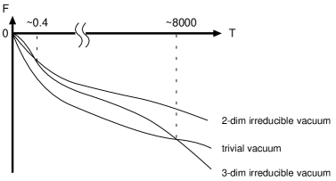
Figure 3: The sketch of free energies in the $N=3$ case.

Namely, once the system is coupled to the heat bath, the degeneracy of vacuum at zero temperature is resolved and the trivial vacuum has the lowest free energy. In the high temperature region $T\sim$ 8000, the three-dimensional irreducible representation of fuzzy sphere is favored rather than trivial vacuum. Thus, the vacuum with the largest irreducible representation of fuzzy sphere is most stable at sufficiently high temperature. This result is the same way as in the irreducible vacuum cases.

It should be noted that we can confirm the behavior of free energies at low and high temperature by using the asymptotic forms. In the low temperature region, the free energies behave as

$$F_{\rm tri}\sim-54T{\rm e}^{-\frac{1}{6T}}\,,\quad F_{\rm 3dim}\sim-6T{\rm e}^{-\frac{1}{6T}}\,,\quad F_{\rm 2dim}\sim-12T{\rm e}^{-\frac{1}{6T}}\,.$$ (3.15)

On the other hand, the high temperature behaviors are described by

$$F_{\rm tri}\sim-81T\ln T\,,\quad F_{\rm 3dim}\sim-89T\ln T\,,\quad F_{\rm 2dim}\sim-48T\ln T\,.$$ (3.16)

These are compatible with the sketch in Fig. 3, and thus we could analytically check the consistency of numerical results.

Next, we shall consider the $N=4$ case. Now we have five types of vacua; i) trivial vacuum, ii) a couple of two-dimensional irreducible fuzzy spheres, iii) four-dimensional irreducible fuzzy sphere, iv) a two-dimensional fuzzy sphere, v) a three-dimensional fuzzy sphere. It is possible to investigate numerically the free energy behaviors as in the $N=3$ case. Because the range of temperature is quite broad and hence we need many graphs of numerical plots, we give only a sketch of the free energies, which is shown in Fig. 4.

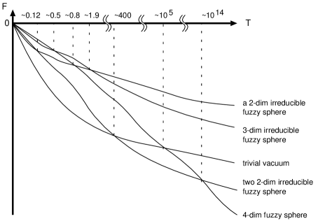
Figure 4: The sketch of free energies in the $N=4$ case.

It can be seen that the trivial vacuum is most stable at low temperature. Then the vacuum with a couple of two-dimensional irreducible fuzzy spheres tend to be preferred from $T\sim 400$. Finally, the four-dimensional irreducible fuzzy sphere is favored at sufficiently high temperature. In the comparison with the $N=3$ case, there is a middle state which is composed of two fuzzy spheres. Thus, we may guess a transition process that $2\times 2$ fuzzy spheres are formed in the trivial vacuum. After this creation process, they would combine each other and form a four-dimensional irreducible representation.

In the present case, it is also possible to confirm the low and high temperature behaviors of free energies by using their asymptotic forms. In the low temperature region, the free energy in each of vacua is expressed as, respectively,

$$F_{\rm tri}\sim-96T{\rm e}^{-\frac{1}{6T}}\,,\quad F_{2\times 2{\rm dim}}\sim-24T{\rm e}^{-\frac{1}{6T}}\,,\quad F_{\rm 4dim}\sim-6T{\rm e}^{-\frac{1}{6T}}\,,$$

$$F_{\rm 2dim}\sim-30T{\rm e}^{-\frac{1}{6T}}\,,\quad F_{\rm 3dim}\sim-12T{\rm e}^{-\frac{1}{6T}}\,.$$ (3.17)

The high temperature behaviors of free energies are

$$F_{\rm tri}\sim-144T\ln T\,,\quad F_{2\times 2{\rm dim}}\sim-156T\ln T\,,\quad F_{\rm 4dim}\sim-159T\ln T\,,$$

$$F_{\rm 2dim}\sim-95T\ln T\,,\quad F_{\rm 3dim}\sim-98T\ln T\,.$$ (3.18)

¿From these asymptotic forms, we can estimate the initial and final behaviors of free energies. As the result, the sketch in Fig. 4 based on numerical studies is confirmed by analytical evaluation.

As a matter of course, we may proceed with the numerical analysis of free energies in the $N\geq 5$ case. We will not carry out here, but it would be possible in principle for a fixed value of $N$ to check that the $2\times 2$ fuzzy spheres are firstly formed as the temperature grows, and then they are combined with each other or enhance to larger irreducible representations. Finally the maximal size irreducible representation would be realized after some transitions. That is, we may argue that an $N$-dimensional irreducible representation dominates a direct sum of small irreducible representations of fuzzy spheres in the $U(N)$ pp-wave matrix model at sufficiently high temperature.

4 Conclusion and Discussion

We have discussed thermodynamics of fuzzy sphere in a matrix model on a pp-wave background. The exact free energy for an arbitrary matrix size $N$ has been computed in the $\mu\rightarrow\infty$ limit. This is a generalization of the result obtained by Huang [7] where the $2\times 2$ matrix formulation [4] was used. We have found that the free energy in the fuzzy sphere vacuum is smaller than that in the trivial vacuum above a critical temperature by carrying out a numerical analysis of free energy with fixed matrix sizes. This result may imply that the fuzzy sphere vacuum is more stable than the trivial vacuum at sufficiently high temperature, and would support that the fluctuations around the trivial vacuum might condense to form fuzzy sphere solutions above the critical temperature.

We have also seen that the critical temperature increases as the matrix size $N$ becomes large. In particular, our evaluation suggests that the change in vacuum type would not happen in the $N\rightarrow\infty$ limit, and it is consistent to the supergravity analysis. In addition, we have found the evidence that an $N$-dimensional irreducible fuzzy sphere (i.e., the largest irreducible representation) is more stable than the reducible one through some numerical plots.

In conclusion, we may argue that a fuzzy sphere vacuum belonging to an $N$-dimensional irreducible representation would dominate above a certain temperature. It is important to give an exact proof for this argument. At any rate, we have to make an effort to clarify whether the critical phenomenon such as a phase transition should exist or not.

It is an interesting future problem to include higher order contributions to our result by computing the energy shift. It is also interesting to study thermodynamics of other classical solutions (For classical solutions in a pp-wave matrix model, for example, see [11, 12, 13]). On the other hand,the trivial vacuum $X=0$ is related to the transverse spherical M5-brane [14]. The five-brane dynamics in the pp-wave matrix model is studied in the recent work [15]. It would be worthwhile to proceed to study in this direction. On the other hand, thermodynamic property of type IIA string theory [16, 17] is studied in [18]. It is also interesting to consider our results from the viewpoint of type IIA string theory. For the study in this direction, a matrix string theory on a pp-wave, which is derived in [16] by using the method [19], would be surely available.

References

- [1] D. Berenstein, J. M. Maldacena and H. Nastase, “Strings in flat space and pp waves from N = 4 super Yang Mills,” JHEP 0204 (2002) 013 [arXiv:hep-th/0202021].
- [2] J. Kowalski-Glikman, “Vacuum states in supersymmetric Kaluza-Klein theory,” Phys. Lett. B 134 (1984) 194.
- [3] R. C. Myers, “Dielectric-branes,” JHEP 9912 (1999) 022 [arXiv:hep-th/9910053].
- [4] K. Sugiyama and K. Yoshida, “Giant graviton and quantum stability in matrix model on PP-wave background,” Phys. Rev. D 66 (2002) 085022 [arXiv:hep-th/0207190].
- [5] H. Shin and K. Yoshida, “One-loop flatness of membrane fuzzy sphere interaction in plane-wave matrix model,” to appear in Nucl. Phys. B, arXiv:hep-th/0309258.
- [6] K. Dasgupta, M. M. Sheikh-Jabbari and M. Van Raamsdonk, “Matrix perturbation theory for M-theory on a PP-wave,” JHEP 0205 (2002) 056 [arXiv:hep-th/0205185].
- [7] W. H. Huang, “Thermal instability of giant graviton in matrix model on pp-wave background,” arXiv:hep-th/0310212.
- [8] K. Sugiyama and K. Yoshida, “Supermembrane on the pp-wave background,” Nucl. Phys. B 644 (2002) 113 [arXiv:hep-th/0206070]; “BPS conditions of supermembrane on the pp-wave,” Phys. Lett. B 546 (2002) 143 [arXiv:hep-th/0206132]; N. Nakayama, K. Sugiyama and K. Yoshida, “Ground state of the supermembrane on a pp-wave,” Phys. Rev. D 68 (2003) 026001, [arXiv:hep-th/0209081].
- [9] T. Kimura and K. Yoshida, “Spectrum of eleven-dimensional supergravity on a pp-wave background,” to appear in Phys. Rev. D, arXiv:hep-th/0307193.
- [10] O. K. Kwon and H. Shin, “Type IIA supergravity excitations in plane-wave background,” Phys. Rev. D 68 (2003) 046007 [arXiv:hep-th/0303153].
- [11] D. Bak, “Supersymmetric branes in PP wave background,” Phys. Rev. D67 (2003) 045017, hep-th/0204033.
- [12] S. Hyun and H. Shin, “Branes from matrix theory in pp-wave background,” Phys. Lett. B543 (2002) 115–120, hep-th/0206090.
- [13] J. H. Park, “Supersymmetric objects in the M-theory on a pp-wave,” JHEP 0210 (2002) 032 [arXiv:hep-th/0208161].
- [14] J. Maldacena, M. M. Sheikh-Jabbari and M. Van Raamsdonk, “Transverse fivebranes in matrix theory,” JHEP 0301 (2003) 038 [arXiv:hep-th/0211139].
- [15] K. Furuuchi, E. Schreiber and G. W. Semenoff, “Five-brane thermodynamics from the matrix model,” arXiv:hep-th/0310286.
- [16] K. Sugiyama and K. Yoshida, “Type IIA string and matrix string on pp-wave,” Nucl. Phys. B 644 (2002) 128 [arXiv:hep-th/0208029].
- [17] S. Hyun and H. Shin, “N = (4,4) type IIA string theory on pp-wave background,” JHEP 0210 (2002) 070 [arXiv:hep-th/0208074].
- [18] S. Hyun, J. D. Park and S. H. Yi, “Thermodynamic behavior of IIA string theory on a pp-wave,” JHEP 0311 (2003) 006 [arXiv:hep-th/0304239].
- [19] Y. Sekino and T. Yoneya, “From supermembrane to matrix string,” Nucl. Phys. B 619 (2001) 22 [arXiv:hep-th/0108176].