Abstract
The quantum dynamics of a bulk-boundary theory is closely examined by the use of the background field method. As an example we take the Mirabelli-Peskin model, which is composed of 5D super Yang-Mills (bulk) and 4D Wess-Zumino (boundary). Singular interaction terms play an important role of canceling the divergences coming from the KK-mode sum. Some new regularization of the momentum integral is proposed. An interesting background configuration of scalar fields is found. It is a localized solution of the field equation. In this process of the vacuum search, we present a new treatment of the vacuum with respect to the extra coordinate. The ”supersymmetric” effective potential is obtained at the 1-loop full (w.r.t. the coupling) level. This is the bulk-boundary generalization of the Coleman-Weinberg’s case. Renormalization group analysis is done and the correct 4D result is reproduced. The Casimir energy is calculated and is compared with the case of the Kaluza-Klein model.

PACS NO:  11.10.Kk, 11.27.+d, 12.60.Jv, 12.10.-g, 11.25.Mj, 04.50.+h

Key Words: bulk-boundary theory, Mirabelli-Peskin model, effective potential, Coleman-Weinberg potential, brane model, Casimir energy, 5D supersymmetry.

1 Introduction

Through recent several years of development, it looks that the higher-dimensional approach has obtained the citizenship as an important building tool in constructing the unified theories. It appears with some names such as ”Randall-Sundrum model”, ”brane world”, ”extra-dimension model”, ”orbifold model”, etc. Before the appearance of the new approach, supersymmetry (SUSY) was the main promising tool to go beyond the standard model. Among many ideas in the higher-dimensional approach, the system of bulk and boundary theories becomes a fascinating model of the unification. A boundary is regarded as our world. It is inspired by the M, string and D-brane theories[1]. One pioneering paper, which concretely describes the model, is that by Mirabelli and Peskin[6]. They take the 5D supersymmetric Yang-Mills theory as a bulk theory and make it couple with a boundary matter. The boundary couplings (with the bulk world) are uniquely fixed by the SUSY requirement. They demonstrated some consistency in the bulk quantum theory by calculating self-energy of the scalar matter field. Here we examine the effective potential and the vacuum energy of this system. We investigate further closely the role of the bulk fields and the singular interactions.

A field theoretical analysis of the bulk and boundary system was recently done in the work by Goldberger and Wise[2]. They try to tackle the problem by the ”generalized” use of the renormalization group. Randall and Schwarts[3, 4] also attacked the same problem by introducing a special regularization of the ultraviolet divergences guided by the idea of the holography. We take a different approach to the bulk and boundary system. (We will see, however, some similar results.) It is, at present, hard to show any consistency ( such as renormalizability, unitarity, etc.) in the higher dimensional quantum field theory. It is, at least perturbatively, unrenormalizable. We would rather regard the bulk world as an external heat-reservoir which gives some ”freedom” to the boundary world and ”define” or ”regularize” the 4D dynamics. The external world of the bulk classically and quantumly affect our world of 4D, and vice versa. In this circumstance we focus on the renormalization properties of the 4D world. We examine a way to treat the linear (power) divergences coming from the bulk quantum effect. Another important aspect is the present treatment of the extra axis. We will find some “freedom” in the definition of the vacuum. $Z^{2}$-symmetry plays an important role there. We can naturally introduce the singular behaviour for some scalars. One important merit of the bulk-boundary approach is that the anomaly phenomenon (of the 4D world) is naturally accepted as a current flow which goes out through the wall or comes into the 4D world.[5].

Contrary to the motivation of the original work of ref.[6], we do not seek the SUSY breaking mechanism, rather we keep the supersymmetry and make use of the SUSY invariant properties in order to make the analysis as simple as possible. The SUSY symmetry is so restrictive that we only need to calculate some small portion of all possible diagrams.

As the analysis of the effective potential of the 5D model, we recall that of the Kaluza-Klein(KK) model[7]. The dynamics quantumly produces the effective potential which describes the Casimir effect. The situation, however, is contrastively different from the present case in some points.
1) The present approach realizes the 4D reduction by the localized (along the extra axis) configuration (kink, soliton, delta-function), whereas KK does it by the shrinkage of the radius of the extra S₁ space.
2) KK does not use Z₂-symmetry whereas the present one exploits it in order to make a singular structure at $x^{5}=0,l$ (fixed points) where the 4D worlds are. The discrete symmetry imposes a nontrivial boundary condition on the vacuum.
3) KK takes the condition scalar field = constant in order to find the vacuum configuration, whereas, in the present case, we do the new treatment of the vacuum by allowing the extra-coordinate dependence on some scalars.
4) The present model is supersymmetric, whereas KK is not.
5) In KK, the scalar field comes from the (5,5)-component of the 5D metric (and partially from the dilaton). The 5D quantum effect produces the effective potential which can be interpreted as the Casimir force induced by the vacuum polarization between the $l$ separated objects. On the other hand, in the present case, the scalar components come from various places: the 5th component of the bulk vector, the bulk scalar and the boundary scalar fields. Hence the vacuum structure becomes much richer.
6)The present model has, as the characteristic length scales, the thickness parameter (brane tension) besides the period of the extra space. As the vacuum energy calculation, we should see the dependence on both lengths.

The present model shares common properties with those of the RS-model in the points such as localization, $Z_{2}$-symmetry, bulk-boundary relation, etc. (The comparative aspect of the KK model and the RS-model is explained in ref.[8].) We could regard the present result about the Casimir energy as some RS counter-part of the result obtained by Appelquist and Chodos for the case of the KK-model.

The concrete object we will obtain is the effective potential. The formalism itself is very orthodox. The new point is its application to the 5D bulk-boundary system. The system is much extended from the ordinary field theory. The effective potential is well-established in the field theory. Especially in the middle of 70’s much literature appeared. One of the famous outcome is the Coleman-E.Weinberg potential[9]. In the SUSY theories, Miller proposed a useful method, called AFTM[10], based on the tadpole diagram method by S. Weinberg[11]. It was applied to unified models[12]. We will take another formalism, the background field method, by B.S. DeWitt[13] and G. t’Hooft[14]. The new formulation of the bulk-boundary system is another aim of this paper.

We summarize the new points as follows:
(1) background-field formulation of the bulk-boundary theory,
(2) $\delta(0)$ singularity problem is solved,
(3) a new proposal for resolving the UV-divergences in the 5D quantum $S^{1}/Z_{2}$ orbifold theory,
(4) new treatment of the vacuum in the presence of the extra-space,
(5) Casimir energy calculation.

Some of the present results are briefly reported in ref.[15].

The paper is organized as follows. In Sec.2, we introduce the present formalism of the background field method, in the analysis of the effective potential. The simple model of Wess-Zumino is taken as an example. Here we explain the ”supersymmetric” effective potential. Mirabelli-Peskin model is explained in Sec.3. It is a typical bulk-boundary model based on 5D SUSY. In Sec.4, we quantize the model using the background field method. A new treatment of the background field, in relation to the extra coordinate, is presented. This leads to an interesting background solution (vacuum) which describes the field-localization. Feynman rules are obtained for the perturbative analysis in Sec.5. The singular vertices, which involve the delta function, appear. Some Feynman diagrams are explicitly calculated. We take into account both bulk and boundary quantum effects. We will find that the singular interaction terms play the role of the ”counter-terms” to cancel the divergences coming from the KK-mode sum. In Sec.6, the mass matrix appearing in the 1-loop Lagrangian is obtained. This is the preparation for the 1-loop full calculation of the next section. Assumption of the form of the background field about its extra-coordinate dependence is crucial for the present analysis. In Sec.7, the effective potential is obtained. Two typical cases, A and B, are considered. In Case A we look at the potential from the vanishing vacuum of the brane matter-field. The final form of the potential is similar to the 4D super QED. In the intermediate stage, we find a new type Casimir energy which is characteristic for the brane world. In Case B, we obtain the potential for the no brane configuration. In the intermediate stage, we find the ordinary type Casimir energy. The effective potential has rich structure. We conclude in Sec.8. We relegate some important detailed explanation to three appendices. App. A treats the super QED which is a good reference point in the analysis of the bulk-boundary theory in the text. App. B provides the calculation of the eigenvalues of the mass matrix of Sec.6. The results are used in Sec.7. App. C explains the concrete form of the present background fields. They satisfy the field equation with the required boundary condition.

2 Effective Potential of Wess-Zumino Model

In order to explain the background field approach to obtain the effective potential, we take the simplest 4D SUSY theory, that is, the Wess-Zumino model:

$${\cal L}[\psi,A,F;\lambda,m]=i\partial_{m}{\bar{\psi}}{\bar{\sigma}}^{m}\psi+{\bar{A}}\partial_{m}\partial^{m}A+{\bar{F}}F$$

$$+[m(AF-{\frac{1}{2}}\psi\psi)+\frac{\lambda}{2}(AAF-\psi\psi A)+\mbox{h.c.}]{\quad,}$$ (1)

where $(\eta^{mn})=\mbox{diag}(-1,1,1,1)$. The notation is basically the same as the textbook by Wess-Bagger[24]. $\psi$ is a Majorana fermion, $A$ is a complex scalar field and $F$ is an (complex scalar) auxiliary field. The general background field method [13, 14, 16] tells us that the (DeWitt-Wilsonian) effective action $S^{eff}[\xi,a,f]$ is given by

$$\exp\{iS^{eff}[\xi,a,f]\}=\int{\cal D}\psi{\cal D}A{\cal D}F$$

$$\times\exp i{\int d^{4}x}\left\{{\cal L}[\xi+\psi,a+A,f+F]-\left.\frac{\delta{\cal L}}{\delta\Phi^{I}}\right|_{b}\Phi^{I}\right\}{\quad,}$$ (2)

where $(\Phi^{I})\equiv(\psi,A,F)$ are the quantum fields and their background fields $(\Phi^{I})|_{b}\equiv(\xi,a,f)$. We define the effective potential $V^{eff}$ as the non-derivative part of $S^{eff}$. A simple and practical way to pick up the part is to consider the case:

$$\xi=0\ ,\ a=\mbox{const.}\ ,\ f=\mbox{const.}{\quad,}$$ (3)

where we put $\xi=0$ from the requirement of the Lorentz invariance of the vacuum and ”const.” means a constant.

$$\exp\{-iV^{eff}[a,f]\}=\exp i\{-V^{eff}_{0}\}$$

$$\times\int{\cal D}\psi{\cal D}A{\cal D}F\exp i{\int d^{4}x}\left\{{\cal L}_{2}+\mbox{order of }(\mbox{quant. field})^{3}\ \right\}{\quad,}$$

$$-V^{eff}_{0}={\bar{f}}f+(ma+\frac{\lambda}{2}a^{2})f+(m{\bar{a}}+\frac{\lambda}{2}{\bar{a}}^{2}){\bar{f}}\equiv{\cal L}_{0}{\quad,}$$

$$\left.\frac{\delta{\cal L}}{\delta\Phi^{I}}\right|_{b}\Phi^{I}=({\bar{f}}+ma+\frac{\lambda}{2}a^{2})F+f\chi A+\mbox{h.c.}\equiv{\cal L}_{1}\ ,\ \chi\equiv m+\lambda a\ ,$$

$${\cal L}_{2}=i\partial_{m}{\bar{\psi}}{\bar{\sigma}}^{m}\psi-{\frac{1}{2}}(\chi\psi\psi+{\bar{\chi}}{\bar{\psi}}{\bar{\psi}})+{\frac{1}{2}}Q^{\dagger}MQ{\quad,}$$

$$M=\left(\begin{array}[]{cccc}\Box&\lambda{\bar{f}}&0&{\bar{\chi}}\\ \lambda f&\Box&\chi&0\\ 0&{\bar{\chi}}&1&0\\ \chi&0&0&1\end{array}\right){\quad,}\quad\Box=\partial_{m}\partial^{m}{\quad,}$$ (8)

where the scalar quantum fields are denoted by the column matrix $Q$: $Q^{T}=(A,{\bar{A}},F,{\bar{F}}),Q^{\dagger}=({\bar{A}},A,{\bar{F}},F)$. The matrix $M$ is the same as the matrix appearing in eq.(15) of Ref.[10]. There is the special case, called on-shell, of the background values $a,f$:

$${\bar{f}}+ma+\frac{\lambda}{2}a^{2}=0{\quad,}\quad\chi f=(m+\lambda a)f=0{\quad,}$$ (9)

which satisfies the field equation and makes ${\cal L}_{1}$ vanish. When the above background values ($a,f$) satisfy the on-shell condition above, $V^{eff}_{0}$ reduces to

$$V^{eff}_{0}|_{\mbox{on-shell}}={\bar{f}}f\geq 0{\quad,}$$ (10)

which shows the positive semi-definiteness. This shows the characteristic aspect of the supersymmetric configuration. The (classical) vacuum is given by: $f={\bar{f}}=0,\ a(m+\frac{\lambda}{2}a)=0\ (a=0\ \mbox{or}\ a=-\frac{2}{\lambda}m)$. In the following, except when explicitly stated, we do not require the on-shell condition (9). We regard $a$ and $f$ not as specific constants (specific vacuum) but as the general source (external) fields appearing in the effective potential. It is an off-shell generalization but is the most natural one based on the background field method.

Let us now evaluate the 1-loop quantum effect. First we can integrate out the auxiliary quantum-fields $F$ and ${\bar{F}}$ using a ”squaring” equation: ${\bar{F}}F+\chi AF+{\bar{\chi}}{\bar{A}}{\bar{F}}=({\bar{F}}+\chi A)(F+{\bar{\chi}}{\bar{A}})-{\bar{\chi}}\chi{\bar{A}}A$. Then the quadratic-part Lagrangian ${\cal L}_{2}$ reduces to ${\cal L}_{2}^{\prime}$:

$${\cal L}_{2}^{\prime}=i\partial_{m}{\bar{\psi}}_{\dot{\alpha}}({\bar{\sigma}}^{m})^{{\dot{\alpha}}\beta}\psi_{\beta}+{\bar{A}}\Box A$$

$$-{\frac{1}{2}}\left(\begin{array}[]{cc}\psi^{\alpha}&{\bar{\psi}}_{\dot{\alpha}}\end{array}\right)\left(\begin{array}[]{cc}\chi\delta_{\alpha}^{\beta}&0\\ 0&{\bar{\chi}}\delta_{\dot{\beta}}^{\dot{\alpha}}\end{array}\right)\left(\begin{array}[]{c}\psi_{\beta}\\ {\bar{\psi}}^{\dot{\beta}}\end{array}\right)\ -{\frac{1}{2}}\left(\begin{array}[]{cc}{\bar{A}}&A\end{array}\right){\bf M}\left(\begin{array}[]{c}A\\ {\bar{A}}\end{array}\right){\quad,}$$ (19)

$${\bf M}=\left(\begin{array}[]{cc}{\bar{\chi}}\chi&-\lambda{\bar{f}}\\ -\lambda f&{\bar{\chi}}\chi\end{array}\right){\quad.}$$ (22)

The eigenvalues of ${\bf M}$ are given as

$$m^{2}_{+}={\bar{\chi}}\chi+\lambda\sqrt{{\bar{f}}f}{\quad,}\quad m^{2}_{-}={\bar{\chi}}\chi-\lambda\sqrt{{\bar{f}}f}{\quad.}$$ (23)

The contribution to the 1-loop effective potential $V^{eff}_{1-loop}$, from the bosonic part ( scalar loop ), is evaluated as

$$\int{\cal D}{\bar{A}}{\cal D}A\exp i{\int d^{4}x}\left\{{\bar{A}}\Box A-{\frac{1}{2}}\left(\begin{array}[]{cc}{\bar{A}}&A\end{array}\right){\bf M}\left(\begin{array}[]{c}A\\ {\bar{A}}\end{array}\right)\right\}$$ (27)

$$=\left[\det(\Box-m_{+}^{2})(\Box-m_{-}^{2})\right]^{-{\frac{1}{2}}}=\exp\left\{-{\frac{1}{2}}{\rm Tr\,}\sum_{i=+,-}\ln(1-\frac{m_{i}^{2}}{\Box})\right\}$$

$$=\exp\left\{-i{\int d^{4}x}V^{eff}_{1-loop}\right\}{\quad.}$$ (28)

The $V^{eff}_{1-loop}$ above lacks the fermionic 1-loop contribution:

$$\int{\cal D}{\bar{\psi}}{\cal D}\psi\exp i{\int d^{4}x}\left\{i\partial_{m}{\bar{\psi}}_{\dot{\alpha}}({\bar{\sigma}}^{m})^{{\dot{\alpha}}\beta}\psi_{\beta}-{\frac{1}{2}}\left(\begin{array}[]{cc}\psi^{\alpha}&{\bar{\psi}}_{\dot{\alpha}}\end{array}\right)\left(\begin{array}[]{cc}\chi\delta_{\alpha}^{\beta}&0\\ 0&{\bar{\chi}}\delta_{\dot{\beta}}^{\dot{\alpha}}\end{array}\right)\left(\begin{array}[]{c}\psi_{\beta}\\ {\bar{\psi}}^{\dot{\beta}}\end{array}\right)\ \right\}$$ (34)

$$=[\det(\Box-{\bar{\chi}}\chi)]^{+1}{\quad.}$$ (35)

This part does not depend on $f$ and ${\bar{f}}$. It says the 1-loop effective potential calculated only by the scalar part is correct up to the $f$-independent terms. As far as the $f$-dependent part is concerned, the scalar part result (28) is sufficient. If we trace the source of this phenomenon, it is simply that the auxiliary fields $f$ and ${\bar{f}}$ have the higher physical dimension, $M^{2}$. They cannot have the Yukawa coupling with fermions. ( $F\psi\psi$ has the mass dimension 5. ) This fact means that $dV^{eff}_{1-loop}/df$ ( or $dV^{eff}_{1-loop}/d{\bar{f}}$ ) is definitely determined only by the scalar part. Miller[10, 17] utilized this fact, that is, F-tadpole or D-tadpole [11] in general SUSY theories are rather simply obtained. In the present case, (1-loop) F-tadpole corresponds to $dV^{eff}_{1-loop}/df$. He noticed, if the SUSY is preserved in the quantization, the $f$-independent part can be fixed by the following boundary condition. We follow Miller’s idea. Looking at the tree-level (on-shell) result (10), and taking into account the quantum stableness of the SUSY theory, we are allowed to take the supersymmetric boundary condition:

$$\mbox{The SUSY effective potential vanishes at}\ f=0.$$ (36)

Normalizing at $f=0$, the 1-loop effective potential is finally obtained as

$$V^{eff}_{1-loop}-V^{eff}_{1-loop}|_{f=0}={\frac{1}{2}}\int\frac{d^{4}k}{(2\pi)^{4}}\ln\left(1-\frac{\lambda^{2}{\bar{f}}f}{(k^{2}+{\bar{\chi}}\chi)^{2}}\right)$$

$$\approx-{\frac{1}{2}}\lambda^{2}{\bar{f}}f\int\frac{d^{4}k}{(2\pi)^{4}}\frac{1}{(k^{2}+m^{2})^{2}}+O(\lambda^{3}){\quad.}$$ (37)

In this simple example, we can explicitly see the subtracting term $-V^{eff}_{1-loop}|_{f=0}$ is just given by the fermion-loop contribution (35). The SUSY condition recovers the ignored (1-loop) contribution in $V^{eff}$. The middle expression of (37) is the same as eq.(26) of Ref.[10] The quadratic divergences appearing in the intermediate stages, as in (28) and (35), cancel and the logarithmic divergence only remain in the final expression (37). It is absorbed by the wave-function renormalization of the auxiliary fields as follows. In order to do the renormalization, we first introduce a counterterm $\Delta{\cal L}$ in the following form.

$$V^{1-loop}_{R}\equiv V^{eff}_{1-loop}-V^{eff}_{1-loop}|_{f=0}-\Delta{\cal L}{\quad,}$$

$$V_{R}\equiv V^{eff}_{0}+V^{1-loop}_{R}{\quad,}\quad V^{eff}_{0}=-{\bar{f}}f+\cdots$$

$$\Delta{\cal L}=\Delta Z\,{\bar{f}}f{\quad,}$$ (38)

where $Z\equiv 1+\Delta Z$ is the wave function renormalization factor of $f$ and ${\bar{f}}$. The 0th (classical) part, $V^{eff}_{0}$, is added. Now we fix $\Delta Z$ by demanding the following renormalization condition.

$$-1\equiv\frac{dV_{R}}{d({\bar{f}}f)}|_{f={\bar{f}}=0,a={\bar{a}}=0}$$

$$=-1-{\frac{1}{2}}\lambda^{2}\int_{|k|\leq\Lambda}\frac{d^{4}k}{(2\pi)^{4}}\frac{1}{(k^{2}+m^{2})^{2}}+\Delta Z{\quad,}$$

$$\mbox{hence }\quad Z\equiv 1+\Delta Z=1-\frac{\lambda^{2}}{16\pi^{2}}\ln\frac{\Lambda}{m}{\quad,}$$ (39)

where $\Lambda$ is the momentum cut-off- $|k^{2}|\leq\Lambda^{2}$. The anomalous dimension of the auxiliary field is given by

$$F_{b}=\sqrt{Z}F{\quad,}\quad$$

$$\mbox{anomalous dimension }\ of\ F\ :\quad\gamma_{F}=\frac{\partial}{\partial\ln\Lambda}\ln Z=-\frac{\lambda^{2}}{16\pi^{2}}+O(\lambda^{4}){\quad.}$$ (40)

We see the quantum effect in the SUSY theory apparently appears in the scaling behaviour of the auxiliary field. It implies the structure(shape) of the effective potential is very sensitive to the quantization. The final form, after the renormalization, is given by

$$V_{R}|_{\mbox{on-shell}}=(V^{eff}_{0}+V^{1-loop}_{R})|_{\mbox{on-shell}}{\quad,}$$

$$V^{eff}_{0}|_{\mbox{on-shell}}={\bar{f}}f{\quad,}$$

$$V^{1-loop}_{R}|_{\mbox{on-shell}}=\frac{1}{64\pi^{2}}\left[-\lambda^{2}{\bar{f}}f-({\bar{\chi}}\chi)^{2}\ln\left\{\frac{({\bar{\chi}}\chi)^{2}}{({\bar{\chi}}\chi-\lambda\sqrt{{\bar{f}}f})({\bar{\chi}}\chi+\lambda\sqrt{{\bar{f}}f})}\right\}\right.$$

$$\left.+2\lambda\,{\bar{\chi}}\chi\,\sqrt{{\bar{f}}f}\ln\left\{\frac{{\bar{\chi}}\chi+\lambda\sqrt{{\bar{f}}f}}{{\bar{\chi}}\chi-\lambda\sqrt{{\bar{f}}f}}\right\}+\lambda^{2}{\bar{f}}f\ln\left\{\frac{({\bar{\chi}}\chi-\lambda\sqrt{{\bar{f}}f})({\bar{\chi}}\chi+\lambda\sqrt{{\bar{f}}f})}{m^{4}}\right\}\right]{\quad,}$$

$$\mbox{where}\quad\quad{\bar{f}}f=|ma+\frac{\lambda}{2}a^{2}|^{2}{\quad,}\quad{\bar{\chi}}\chi=|m+\lambda a|^{2}{\quad.}$$ (41)

For the pure imaginary case of $a=ib$ ($b$ is a real number), the above potentials, $V^{eff}_{0}|_{\mbox{on-shell}}$ and $V^{1-loop}_{R}|_{\mbox{on-shell}}$, are depicted in Fig.1. In this case we have ${\bar{f}}f=m^{2}b^{2}+\frac{\lambda^{2}}{4}b^{4}{\quad,}\quad{\bar{\chi}}\chi=m^{2}+\lambda^{2}b^{2}$. The precise shape of the quantum correction depends on the renormalization condition. However some characteristic features are considered meaningful. The shape of the 1-loop correction is not the Coleman-Weinberg type. The total shape of $V^{1-loop}_{R}|_{\mbox{on-shell}}$ is similar to the tree potential $V^{eff}_{0}|_{\mbox{on-shell}}$. This shows that the SUSY invariant vacuum, $b=0$, is stable against the quantum effect.

Figure 1: The effective potential of the Wess-Zumino model(41). The case $a=ib$($b$: real) and the mass parameter $m=1$. The tree part ($V^{eff}_{0}|_{\mbox{on-shell}}\equiv V_{0}$, left) and the 1-loop correction part ($V^{1-loop}_{R}|_{\mbox{on-shell}}\equiv V_{1}$, right) are depicted for the coupling parameter $\lambda=0.1$(up), $\lambda=1$(down). The horizontal axis is $b$. The potentials are even functions of $b$.

The positive definiteness is preserved after the 1-loop correction. The form of the potential does not essentially change. This result typically shows a general feature of SUSY theories. It was confirmed before in the counter-term calculation[21].

Super QED is similarly treated in Appendix A. In this case the matter sector is vector-like by introducing a pair of chiral multiplets. The SUSY boundary condition is taken at D=0. The anomalous dimension of the D-field and the $\beta$-function of the coupling are obtained. The 1-loop effective potential is explicitly obtained and its SUSY invariant properties are confirmed. The result will become an important reference in the analysis of the bulk-boundary theory in the following sections.

3 Mirabelli-Peskin Model

As a toy model of a bulk-boundary model, Mirabelli and Peskin proposed the following system. Let us consider the 5 dimensional space-time. The space of the fifth component is taken to be $S_{1}$, with the periodicity $2l$.

$${x^{5}}\rightarrow{x^{5}}+2l{\quad.}$$ (42)

We also require the system to be (anti)symmetric with respect to the $Z_{2}$-symmetry:

$$Z_{2}\mbox{ transformation}:\ x^{5}\rightarrow-x^{5}{\quad.}$$ (43)

This makes the two points, ${x^{5}}=0$ and ${x^{5}}=l$, fixed points under $Z_{2}$-transformation. The extra space is $S^{1}/Z_{2}$ orbifold. Let us consider 5D bulk theory ${\cal L}_{bulk}$ which is coupled with 4D matter theory ${\cal L}_{bnd}$ on a ”wall” at ${x^{5}}=0$ and with ${\cal L}^{\prime}_{bnd}$ on the other ”wall” at ${x^{5}}=l$. The boundary Lagragians are, in the bulk action, described by the delta-functions along the extra axis $x^{5}$.

$$S=\int d^{5}x\{{\cal L}_{blk}+\delta(x^{5}){\cal L}_{bnd}+\delta(x^{5}-l){{\cal L}^{\prime}}_{bnd}\}{\quad.}$$ (44)

We make use of the SUSY symmetry in order to make the problem simple. Both bulk and boundary quantum effects are taken into account.

(i) 5D super Yang-Mills theory
 We take, as the bulk dynamics, the 5D super YM theory which is made of a vector field $A^{M}\ (M=0,1,2,3,5)$, a scalar field $\Phi$, a doublet of symplectic Majorana fields $\lambda^{i}\ (i=1,2)$, and a triplet of auxiliary scalar fields $X^{a}\ (a=1,2,3)$. The metric is $(\eta_{MN})=\mbox{diag}(-1,1,1,1,1)$. We basically follow the notation of [22].

$${\cal L}_{SYM}={\rm tr\,}\left(-{\frac{1}{2}}{F_{MN}}^{2}-(\nabla_{M}\Phi)^{2}-i{\bar{\lambda}}_{i}\gamma^{M}\nabla_{M}\lambda^{i}+(X^{a})^{2}+g{\bar{\lambda}}_{i}[\Phi,\lambda^{i}]\right){\quad,}$$

$$F_{MN}=\partial_{M}A_{N}-\partial_{N}A_{M}+ig[A_{M},A_{N}]{\quad,}\quad\nabla_{M}\Phi=\partial_{M}\Phi+ig[A_{M},\Phi]{\quad,}$$

$$\nabla_{M}\lambda^{i}=\partial_{M}\lambda^{i}+ig[A_{M},\lambda^{i}]{\quad,}$$ (45)

where all bulk fields are the adjoint representation of the gauge group $G$. The SU(2)${}_{\mbox{R}}$ index $i$ is raised and lowered by the anti-symmetric tensors $\epsilon^{ij}$ and $\epsilon_{ij}$.

$$A_{M}=A_{M\alpha}T^{\alpha}{\quad,}\quad\Phi=\Phi_{\alpha}T^{\alpha}{\quad,}\quad\lambda^{i}=\lambda^{i}_{\alpha}T^{\alpha}{\quad,}\quad X^{a}=X^{a}_{\alpha}T^{\alpha}{\quad,}$$

$$\quad[T^{\alpha},T^{\beta}]=if^{{\alpha\beta}\gamma}T^{\gamma}{\quad,}\quad{\rm tr\,}(T^{\alpha}T^{\beta})={\frac{1}{2}}\delta^{\alpha\beta}{\quad,}$$ (46)

where $T^{\alpha}$ is the generator of the group and $f^{{\alpha\beta}\gamma}$ is the structure constant. ( As for the group indices $\alpha,\beta,\cdots$, there is no distinction between the upper one and the lower one. ) The bulk Lagrangian ${\cal L}_{SYM}$ of (45) is invariant under the following SUSY transformation.

$$\delta_{\xi}A^{M}=i{\bar{\xi}}_{i}\gamma^{M}\lambda^{i}{\quad,}$$

$$\delta_{\xi}\Phi=i{\bar{\xi}}_{i}\lambda^{i}{\quad,}$$

$$\delta_{\xi}\lambda^{i}=(\Sigma^{MN}F_{MN}+\gamma^{M}\nabla_{M}\Phi)\xi^{i}+i(X^{a}\sigma^{a})^{i}_{~{}j}\xi^{j}{\quad,}$$

$$\delta_{\xi}X^{a}={\bar{\xi}}_{i}(\sigma^{a})^{i}_{~{}j}\gamma^{M}\nabla_{M}\lambda^{j}+i[\Phi,{\bar{\xi}}_{i}(\sigma^{a})^{i}_{~{}j}\lambda^{j}]{\quad,}$$ (47)

where $\Sigma^{MN}=\frac{1}{4}[\gamma^{M},\gamma^{N}]$, and the SUSY global parameter $\xi^{i}$ is the symplectic Majorana spinor. This system has the symmetry of 8 real super charges.

As the 5D gauge-fixing term, we take the Feynman gauge:

$${\cal L}_{gauge}=-{\rm tr\,}(\partial_{M}A^{M})^{2}=-{\frac{1}{2}}(\partial_{M}A^{M}_{~{}\alpha})^{2}{\quad.}$$ (48)

The corresponding ghost Lagrangian is given by

$${\cal L}_{ghost}=-2\,{\rm tr\,}\partial_{M}{\bar{c}}\cdot\nabla^{M}(A)c=-2\,{\rm tr\,}\partial_{M}{\bar{c}}\cdot(\partial^{M}c+ig[A^{M},c]){\quad,}$$ (49)

where $c$ and ${\bar{c}}$ are the complex ghost fields. We take the following bulk action.

$${\cal L}_{blk}={\cal L}_{SYM}+{\cal L}_{gauge}+{\cal L}_{ghost}{\quad.}$$ (50)

(ii) $Z_{2}$-structure
 In order to consistently project out ${\cal N}=1$ SUSY multiplet which has 4 real super charges(4Q’s), we make use of the $Z_{2}$ symmetry (43) which divides the 8 $Q^{\prime}s$ system into two 4Q’s systems. We assign $Z_{2}$-parity, even ($P=+1$) or odd ($P=-1$) under the $Z_{2}$-transformation, to all fields in accordance with the 5D SUSY (47). A consistent choice is given as in Table 1. Note that $A^{m},(m=0,1,2,3)$, is the 4D components of the bulk vector$A^{M}$. A symplectic Majorana field is expressed by two Weyl spinors. We can write $\lambda^{i}$ and $\xi^{i}$ as follows:

$$\lambda^{1}=\left(\begin{array}[]{c}(\lambda_{L})_{\alpha}\\ ({\bar{\lambda}}_{R})^{\dot{\alpha}}\end{array}\right){\quad,}\quad\lambda^{2}=\left(\begin{array}[]{c}(\lambda_{R})_{\alpha}\\ -({\bar{\lambda}}_{L})^{\dot{\alpha}}\end{array}\right){\quad,}\quad\xi^{1}=\left(\begin{array}[]{c}(\xi_{L})_{\alpha}\\ ({\bar{\xi}}_{R})^{\dot{\alpha}}\end{array}\right){\quad,}\quad\xi^{2}=\left(\begin{array}[]{c}(\xi_{R})_{\alpha}\\ -({\bar{\xi}}_{L})^{\dot{\alpha}}\end{array}\right){\quad.}$$ (59)

$$\begin{array}[]{|c|c|c|}\hline\cr&P=+1\ ,\ \xi_{L}&P=-1\ ,\ \xi_{R}\\ \hline\cr A^{M}&A^{m}&A^{5}\\ \hline\cr\Phi&-&\Phi\\ \hline\cr\lambda^{i}&\lambda_{L}&\lambda_{R}\\ \hline\cr X^{a}&X^{3}&X^{1,2}\\ \hline\cr\lx@intercol\hfil\hfil\lx@intercol\\ \lx@intercol\hfil Table\ 1\ \ Z_{2}-parity~{}assignment.\hfil\lx@intercol\\ \end{array}$$

${\cal L}_{SYM}$ of (45) is invariant under the $Z_{2}$-transformation (43). On the wall ($x^{5}=0$), all odd-parity states vanish. The parity odd fields, $A^{5}$ and $\Phi$ in Table 1, will play an important role in the effective potential. The SUSY transformation (47) reduces to the following one of even-parity states generated by $\xi_{L}$:

$$\delta_{\xi}A^{m}=i{\bar{\xi}}_{L}{\bar{\sigma}}^{m}\lambda_{L}+i\xi_{L}\sigma^{m}{\bar{\lambda}}_{L}{\quad,}$$

$$\delta_{\xi}\lambda_{L}=\sigma^{mn}F_{mn}\xi_{L}+i(X^{3}-\nabla_{5}\Phi)\xi_{L}{\quad,}$$

$$\delta_{\xi}(X^{3}-\nabla_{5}\Phi)={\bar{\xi}}_{L}{\bar{\sigma}}^{m}\nabla_{m}\lambda_{L}-\xi_{L}\sigma^{m}\nabla_{m}{\bar{\lambda}}_{L}{\quad.}$$ (60)

(Note that the odd parity field $\Phi$ appears in the ${x^{5}}$-derivative form.) This is a ${\cal N}=1$ (4D) vector multiplet ($A^{m},\lambda_{L},X^{3}-\nabla_{5}\Phi$) transformation in the WZ-gauge although all fields depend on the extra coordinate ${x^{5}}$. Especially ${\cal D}\equiv X^{3}-\nabla_{5}\Phi$ plays the role of D-field. The multiplet defined in the 5D world can be expressed in the form of the 4D vector superfied.

$$V=-\theta\sigma^{m}{\bar{\theta}}A_{m}+i\theta^{2}{\bar{\theta}}{\bar{\lambda}}_{L}-i{\bar{\theta}}^{2}\theta\lambda_{L}+{\frac{1}{2}}\theta^{2}{\bar{\theta}}^{2}{\cal D}{\quad,}\quad{\cal D}=X^{3}-\nabla_{5}\Phi{\quad.}$$ (61)

The odd-parity fields $(\Phi+iA_{5},-i\sqrt{2}\lambda_{R},X^{1}+iX^{2})$ transform as a chiral (adjoint) multiplet.

$$\delta_{\xi}(\Phi+iA_{5})=\sqrt{2}\xi_{L}(-i\sqrt{2}\lambda_{R}){\quad,}$$

$$\delta_{\xi}\lambda_{R}=(i\sigma^{m}F_{5m}-\sigma^{m}\nabla_{m}\Phi){\bar{\xi}}_{L}+i(X^{1}+iX^{2})\xi_{L}{\quad,}$$

$$\delta_{\xi}(X^{1}+iX^{2})=2{\bar{\xi}}_{L}({\bar{\sigma}}^{m}\nabla_{m}\lambda_{R}-i\nabla_{5}{\bar{\lambda}}_{L})-2i[\Phi,{\bar{\xi}}_{L}{\bar{\lambda}}_{L}]{\quad.}$$ (62)

This multiplet can be expressed in the 4D superspace as

$$\Sigma=(\Phi+iA_{5})+\sqrt{2}\theta(-i\sqrt{2}\lambda_{R})+\theta^{2}(X^{1}+iX^{2}){\quad.}$$ (63)

We will not use this multiplet in this paper.

iii) Matter Lagrangian on the wall

Let us introduce matter fields on the walls. We consider two cases: a) chiral matter,  b) vector-like matter.

iiia) Chiral matter
 We introduce, on the ${x^{5}}=0$ brane, a 4 dim chiral multiplet ($\phi,\psi,F$) where $\phi$ is a complex scalar field, $\psi$ is a Weyl spinor and $F$ is an auxiliary field of complex scalar. This is the simplest case as a matter candidate and was taken in the original theory[6]. The chiral superfield $\Theta$ is introduced :

$$\Theta=\phi+\sqrt{2}\theta\psi+\theta^{2}F{\quad,}\quad{\bar{\Theta}}=\phi^{\dagger}+\sqrt{2}{\bar{\theta}}{\bar{\psi}}+{\bar{\theta}}^{2}F^{\dagger}{\quad.}$$ (64)

Using the ${\cal N}=1$ SUSY property of the bulk fields ($A^{m},\lambda_{L},{\cal D}=X^{3}-\nabla_{5}\Phi$), we can find the bulk-boundary coupling.

$${\cal L}^{(a)}_{bnd}=\left.{\bar{\Theta}}{\rm e}^{2gV}\Theta\right|_{\theta^{2}{\bar{\theta}}^{2}}=-\nabla_{m}\phi^{\dagger}\nabla^{m}\phi-i{\bar{\psi}}{\bar{\sigma}}^{m}\nabla_{m}\psi+F^{\dagger}F$$

$$+\sqrt{2}ig({\bar{\psi}}{\bar{\lambda}}_{L}\phi-\phi^{\dagger}\lambda_{L}\psi)+g\phi^{\dagger}{\cal D}\phi{\quad,}$$ (65)

where $\nabla_{m}\equiv\partial_{m}+igA_{m},\ {\cal D}=X^{3}-\nabla_{5}\Phi$. All matter fields are taken to be the fundamental representation of the internal group G. We may add the following superpotential term to the above Lagrangian.

$${\cal L}_{SupPot}=({\frac{1}{2}}m_{{\alpha^{\prime}}{\beta^{\prime}}}\Theta_{\alpha^{\prime}}\Theta_{\beta^{\prime}}+\frac{1}{3!}\lambda_{{\alpha^{\prime}}{\beta^{\prime}}{\gamma^{\prime}}}\Theta_{\alpha^{\prime}}\Theta_{\beta^{\prime}}\Theta_{\gamma^{\prime}})|_{\theta^{2}}+\mbox{h.c.}{\quad,}$$ (66)

where the primed Greek suffixes (${\alpha^{\prime}},{\beta^{\prime}},\cdots$) show those of the fundamental representation.

iiib) Vector-like matter
 We introduce, as the 4D matter fields on the ${x^{5}}=0$ brane, one pair of 4 dim chiral multiplets, $\Theta_{S}$=($\phi_{S},\psi_{S},F_{S}$) and $\Theta_{R}$=($\phi_{R},\psi_{R},F_{R}$).

$${\cal L}^{(b)}_{bnd}=\left.\left({\bar{\Theta}}_{S}{\rm e}^{2gV}\Theta_{S}+{\bar{\Theta}}_{R}{\rm e}^{-2gV}\Theta_{R}\right)\right|_{\theta^{2}{\bar{\theta}}^{2}}+m(\Theta_{S}\Theta_{R}|_{\theta^{2}}+{\bar{\Theta}}_{S}{\bar{\Theta}}_{R}|_{{\bar{\theta}}^{2}})$$

$$=-(\nabla^{+}_{m}\phi_{S})^{\dagger}(\nabla^{m}_{+}\phi_{S})-(\nabla^{-}_{m}\phi_{R})^{\dagger}(\nabla^{m}_{-}\phi_{R})+F^{\dagger}_{S}F_{S}+F^{\dagger}_{R}F_{R}$$

$$-{\frac{1}{2}}({\bar{\psi}}_{S}i{\bar{\sigma}}^{m}\nabla^{+}_{m}\psi_{S}+{\bar{\psi}}_{R}i{\bar{\sigma}}^{m}\nabla^{-}_{m}\psi_{R}+\mbox{h.c.})$$

$$+\sqrt{2}g(i{\bar{\psi}}_{S}{\bar{\lambda}}_{L}\phi_{S}-i{\bar{\psi}}_{R}{\bar{\lambda}}_{L}\phi_{R}+\mbox{h.c.})$$

$$+g(\phi^{\dagger}_{S}D\phi_{S}-\phi^{\dagger}_{R}D\phi_{R})+m\{\phi_{S}F_{R}+\phi_{R}F_{S}-\psi_{S}\psi_{R}+\mbox{h.c.}\}{\quad,}$$ (67)

where $\nabla^{\pm}_{m}=\partial_{m}\pm igA_{m}$. This is the bulk-boundary generalization of super QED or QCD. We can identify the matter fermions $(\psi_{S},\psi_{R})$ as one Dirac fermion (”electron, quark”).

On the other brane ${x^{5}}=l$, we introduce another WZ-multiplet(s), $(\phi^{\prime},\psi^{\prime},F^{\prime})$ for case a), and $(\phi_{S}^{\prime},\psi_{S}^{\prime},F_{S}^{\prime})$ and $(\phi_{R}^{\prime},\psi_{R}^{\prime},F_{R}^{\prime})$ for case b). The bulk-boundary couplings are fixed in the same way. The quadratic (kinetic) terms of the vector $A^{m}$, the gaugino spinor $\lambda_{L}$ and ${\cal D}=X^{3}-\nabla_{5}\Phi$ are in the bulk world. We note here the interaction between the bulk fields and the boundary ones is definitely fixed from SUSY. In the ordinary standpoint of the field theory, the boundary theory (65) or (67) is perturbatively unrenormalizable because the coupling $g$ has the physical dimension of $M^{-1/2}$ (unrenormalizable coupling).

4 Quantization Using Background Field Method

From the results of Sect.2 (and App.A), we may put, for the purpose of obtaining the 1-loop effective potential, the following conditions on ${\cal L}_{blk}$:

$$A^{m}=0\ (m=0,1,2,3){\quad,}\quad\lambda^{i}={\bar{\lambda}}^{i}=0{\quad.}$$ (68)

Here the extra (fifth) component of the bulk vector $A^{5}$ does not taken to be zero because it is regarded as a 4D scalar on the wall. Then ${\cal L}_{blk}={\cal L}^{SYM}+{\cal L}_{gauge}+{\cal L}_{ghost}$ reduces to

$${\cal L}^{red}_{blk}[\Phi,X^{3},A_{5}]\quad\quad\quad\quad\quad\quad\quad\quad\quad\quad\quad\quad\quad\quad\quad\quad\quad\quad$$

$$={\rm tr\,}\left\{-\partial_{M}\Phi\partial^{M}\Phi+X^{3}X^{3}-\partial_{M}A_{5}\partial^{M}A_{5}+2g(\partial_{5}\Phi\times A_{5})\Phi-g^{2}(A_{5}\times\Phi)(A_{5}\times\Phi)\right\}$$

$$+{\cal L}^{red}_{ghost}[c,{\bar{c}},A_{5}]+\mbox{irrel. terms}{\quad,}$$

$${\cal L}^{red}_{ghost}[c,{\bar{c}},A_{5}]=-2{\rm tr\,}\{\partial_{m}{\bar{c}}\cdot\partial^{m}c+\partial_{5}{\bar{c}}\cdot(\partial^{5}c+ig[A^{5},c])\}{\quad,}$$ (69)

where we have dropped terms of $X^{1}_{\alpha}X^{1}_{\alpha},X^{2}_{\alpha}X^{2}_{\alpha}$ as ’irrelevant terms’ because they decouple from other fields. As for the boundary part, we may impose the conditions:

$$\mbox{a. Chiral matter : }A^{m}=0{\quad,}\quad\psi=0{\quad,}\quad\lambda_{L}=0\ ;$$

$$\mbox{b. vector-like matter : }A^{m}=0{\quad,}\quad\psi_{S}=\psi_{R}=0{\quad,}\quad\lambda_{L}=0{\quad.}$$ (70)

${\cal L}_{bnd}$ reduces to

a. Chiral matter

$${\cal L}^{red}_{bnd(a)}[\phi,\phi^{\dagger},{\cal D}=X^{3}-\nabla_{5}\Phi]=$$

$$-\partial_{m}\phi^{\dagger}\partial^{m}\phi+g(X^{3}_{\alpha}-\partial_{5}\Phi_{\alpha}+gf^{\alpha\beta\gamma}A_{5\beta}\Phi_{\gamma})\phi^{\dagger}_{\beta^{\prime}}(T^{\alpha})_{{\beta^{\prime}}{\gamma^{\prime}}}\phi_{\gamma^{\prime}}+F^{\dagger}F$$

$$+\left\{\frac{m_{{\alpha^{\prime}}{\beta^{\prime}}}}{2}(\phi_{\alpha^{\prime}}F_{\beta^{\prime}}+F_{\alpha^{\prime}}\phi_{\beta^{\prime}})+\frac{\lambda_{{\alpha^{\prime}}{\beta^{\prime}}{\gamma^{\prime}}}}{3!}(\phi_{\alpha^{\prime}}\phi_{\beta^{\prime}}F_{\gamma^{\prime}}+\phi_{\alpha^{\prime}}F_{\beta^{\prime}}\phi_{\gamma^{\prime}}+F_{\alpha^{\prime}}\phi_{\beta^{\prime}}\phi_{\gamma^{\prime}})+\mbox{h.c.}\right\}{\quad.}$$

b. Vector-like matter

$${\cal L}^{red}_{bnd(b)}[\phi_{S},\phi_{S}^{\dagger},\phi_{R},\phi_{R}^{\dagger},{\cal D}=X^{3}-\nabla_{5}\Phi]=-\partial_{m}\phi_{S}^{\dagger}\partial^{m}\phi_{S}-\partial_{m}\phi_{R}^{\dagger}\partial^{m}\phi_{R}$$

$$+g(X^{3}_{\alpha}-\nabla_{5}\Phi_{\alpha})(T^{\alpha})_{{\beta^{\prime}}{\gamma^{\prime}}}(\phi^{\dagger}_{S{\beta^{\prime}}}\phi_{S{\gamma^{\prime}}}-\phi^{\dagger}_{R{\beta^{\prime}}}\phi_{R{\gamma^{\prime}}})+F^{\dagger}_{S}F_{S}+F^{\dagger}_{R}F_{R}+m(\phi_{S}F_{R}+\phi_{R}F_{S}+\mbox{h.c.}){\quad,}$$ (71)

where ${\alpha^{\prime}},{\beta^{\prime}}$ are the suffixes of the fundamental representation. In the same way, the boundary Lagrangians at ${x^{5}}=l$, ${\cal L}^{\prime}_{bnd(a)}$ and ${\cal L}^{\prime}_{bnd(b)}$, reduce to ${\cal L}^{{}^{\prime}red}_{bnd(a),(b)}=(\phi\rightarrow\phi^{\prime},F\rightarrow F^{\prime}\mbox{in (\ref{ep4})})$. Now we expand all scalar fields ($\Phi,X^{3},A_{5};\phi,F,\phi^{\prime},F^{\prime}$) , except ghost fields, into the quantum fields (which are denoted again by the same symbols) and the background fields ($\varphi,\chi^{3},a_{5};\eta,f,\eta^{\prime},f^{\prime}$).

$$\Phi\rightarrow\varphi+\Phi{\quad,}\quad X^{3}\rightarrow\chi^{3}+X^{3}{\quad,}\quad A_{5}\rightarrow a_{5}+A_{5}{\quad,}$$

$$\left\{\begin{array}[]{cc}\phi\rightarrow\eta+\phi,F\rightarrow f+F\mbox{ and primed ones}&\mbox{chiral matter}\\ \phi_{S}\rightarrow\eta_{S}+\phi_{S},\phi_{R}\rightarrow\eta_{R}+\phi_{R},F_{S}\rightarrow f_{S}+F_{S},F_{R}\rightarrow f_{R}+F_{R}&\mbox{vector-like}\\ \mbox{ and primed ones}&\mbox{matter}\end{array}\right.$$ (75)

We treat the ghost fields as quantum ones.

In Sec.2, for the purpose of obtaining the effective potential we consider the case that the background fields are constant (in order to pick up the non-derivative part of the effective action). In the present case of the 5D space-time, we have the extra coordinate ${x^{5}}$. Because 4D($x^{m}$-space) scalar property is independent of the extra space, we take into account the ${x^{5}}$-dependency of the vacuum configuration. The distribution along the extra coordinate is important to make the localization configuration. We require that the background fields may be constant only in 4D world, not necessarily in 5D world. We may allow the background field to depend on the extra coordinate $x^{5}$. This gives us an interesting possibility to the extra space model . (See also the beginning paragraph of Sec.6 where the necessity of the present treatment is explained using an explicitly-${x^{5}}$-dependent solution (101).)

When the background fields ($\varphi,\chi^{3},a_{5};\eta,f,\eta^{\prime},f^{\prime}$) satisfy the field equations derived from ${\cal L}^{red}_{blk}+\delta({x^{5}}){\cal L}^{red}_{bnd}+\delta({x^{5}}-l){\cal L}^{{}^{\prime}red}_{bnd}$ , using (69) and (71), the situation is called ”on-shell”. The equations (on-shell condition) are given as,

$$\delta\Phi_{\alpha}\quad;$$

$${\partial_{5}}^{2}\varphi_{\alpha}+gf_{\beta\gamma\alpha}\partial_{5}\varphi_{\beta}a_{5\gamma}-gf_{{\alpha\beta}\gamma}\partial_{5}(a_{5\beta}\varphi_{\gamma})-g^{2}f_{\beta\alpha\tau}f_{\gamma\delta\tau}a_{5\beta}a_{5\gamma}\varphi_{\delta}$$

$$+g\partial_{5}\delta({x^{5}})\,\eta^{\dagger}T^{\alpha}\eta+g\partial_{5}\delta({x^{5}}-l)\,\eta^{{}^{\prime}{\dagger}}T^{\alpha}\eta^{\prime}+g^{2}(\delta({x^{5}})\eta^{\dagger}T^{\gamma}\eta+\delta({x^{5}}-l)\eta^{{}^{\prime}{\dagger}}T^{\gamma}\eta^{\prime})f^{\beta\alpha\gamma}a_{5\beta}$$

$$=-\partial_{5}Z_{\alpha}-g(Z\times a_{5})_{\alpha}=0,$$

$$\delta A_{5\alpha}\quad;$$

$${\partial_{5}}^{2}a_{5\alpha}+gf_{\beta\alpha\gamma}\partial_{5}\varphi_{\beta}\,\varphi_{\gamma}-g^{2}f_{{\alpha\beta}\tau}f_{\gamma\delta\tau}\varphi_{\beta}a_{5\gamma}\varphi_{\delta}+g^{2}(\delta({x^{5}})\eta^{\dagger}T^{\gamma}\eta+\delta({x^{5}}-l)\eta^{{}^{\prime}{\dagger}}T^{\gamma}\eta^{\prime})f^{\alpha\beta\gamma}\varphi_{\beta}$$

$$={\partial_{5}}^{2}a_{5\alpha}-g(\varphi\times Z)_{\alpha}=0\ ,$$

$$\delta X^{3}_{\alpha}\quad;$$

$$\chi^{3}_{\alpha}+g(\delta({x^{5}})\eta^{\dagger}T^{\alpha}\eta+\delta({x^{5}}-l)\eta^{{}^{\prime}{\dagger}}T^{\alpha}\eta^{\prime})=0\ ,$$

$$\delta\phi^{\dagger}_{\alpha^{\prime}}\quad(\delta\phi^{{}^{\prime}{\dagger}}_{\alpha^{\prime}})\quad;$$

$$d_{\beta}(T^{\beta}\eta)_{\alpha^{\prime}}+m_{{\alpha^{\prime}}{\beta^{\prime}}}f^{\dagger}_{\beta^{\prime}}+{\frac{1}{2}}\lambda_{{\alpha^{\prime}}{\beta^{\prime}}{\gamma^{\prime}}}\eta^{\dagger}_{\beta^{\prime}}f^{\dagger}_{\gamma^{\prime}}=0\ ,\quad(\eta\rightarrow\eta^{\prime},f\rightarrow f^{\prime}\ \mbox{ in the left eq.})$$

$$\delta F^{\dagger}_{\alpha^{\prime}}\quad(\delta F^{{}^{\prime}{\dagger}}_{\alpha^{\prime}})\quad;$$

$$f_{\alpha^{\prime}}+m_{{\alpha^{\prime}}{\beta^{\prime}}}\eta^{\dagger}_{\beta^{\prime}}+{\frac{1}{2}}\lambda_{{\alpha^{\prime}}{\beta^{\prime}}{\gamma^{\prime}}}\eta^{\dagger}_{\beta^{\prime}}\eta^{\dagger}_{\gamma^{\prime}}=0{\quad,}\quad(\eta\rightarrow\eta^{\prime},f\rightarrow f^{\prime}\ \mbox{ in the left eq.}){\quad,}$$ (76)

where $d_{\alpha}=(\chi^{3}-\partial_{5}\varphi+ga_{5}\times\varphi)_{\alpha}$ is the background (4 dimensional) D-field and $Z_{\alpha}\equiv-g(\delta({x^{5}})\eta^{\dagger}T^{\alpha}\eta+\delta({x^{5}}-l)\eta^{{}^{\prime}{\dagger}}T^{\alpha}\eta^{\prime})-\partial_{5}\varphi_{\alpha}+gf_{{\alpha\beta}\gamma}a_{5\beta}\varphi_{\gamma}$. In deriving the above equations, we assume, based on the statement of the previous paragraph on the background field, $\varphi=\varphi({x^{5}}),\chi^{3}=\chi^{3}({x^{5}}),a_{5}=a_{5}({x^{5}}),\eta=\mbox{const},\eta^{\prime}=\mbox{const}$. The total symmetricity of $m_{{\alpha^{\prime}}{\beta^{\prime}}}$ and $\lambda_{{\alpha^{\prime}}{\beta^{\prime}}{\gamma^{\prime}}}$ with respect to the suffixes is also assumed. In the above derivation, we use the fact that total divergences vanish from the periodicity condition. As stated below (10), we do not assume the above on-shell condition except when we state its use. We regard the background fields as general external fields or as off-shell fields.

The quadratic part w.r.t. the quantum fields ($\Phi,X^{3},A_{5};\phi,F,\phi^{\prime},F^{\prime}$) gives us the 1-loop quantum effect. That part of ${\cal L}^{red}_{blk}$ is given as

$${\cal L}^{2}_{blk}[\Phi,A_{5},X^{3}]={\rm tr\,}\,\{-\partial_{M}\Phi\partial^{M}\Phi+X^{3}X^{3}-\partial_{M}A_{5}\partial^{M}A_{5}\}$$

$$+2g\,{\rm tr\,}\left[(\partial_{5}\varphi\times A_{5})\Phi+(\partial_{5}\Phi\times a_{5})\Phi+(\partial_{5}\Phi\times A_{5})\varphi\right]$$

$$-2g^{2}{\rm tr\,}\left[(a_{5}\times\varphi)(A_{5}\times\Phi)\right]-g^{2}{\rm tr\,}(a_{5}\times\Phi+A_{5}\times\varphi)^{2}+{\cal L}^{2}_{ghost}[c,{\bar{c}}]{\quad,}$$

$${\cal L}^{2}_{ghost}[c,{\bar{c}}]=-2{\rm tr\,}\{\partial_{m}{\bar{c}}\cdot\partial^{m}c+\partial_{5}{\bar{c}}\cdot(\partial^{5}c+ig[a^{5},c])\}{\quad.}$$ (77)

The quadratic part of ${\cal L}^{red}_{bnd}$ is given by

$${\cal L}^{2}_{bnd(a)}[\phi,\phi^{\dagger},F,F^{\dagger};\Phi,A_{5},X^{3}]=-\partial_{m}\phi^{\dagger}\partial^{m}\phi+gd_{\alpha}\phi^{\dagger}T^{\alpha}\phi-ig^{2}[A_{5},\Phi]_{\alpha}\eta^{\dagger}T^{\alpha}\eta$$

$$+g(X^{3}_{\alpha}-\partial_{5}\Phi_{\alpha}-ig[a_{5},\Phi]_{\alpha}-ig[A_{5},\varphi]_{\alpha})(\eta^{\dagger}T^{\alpha}\phi+\phi^{\dagger}T^{\alpha}\eta)+F^{\dagger}F$$

$$+\{m_{{\alpha^{\prime}}{\beta^{\prime}}}\phi_{\alpha^{\prime}}F_{\beta^{\prime}}+\frac{\lambda_{{\alpha^{\prime}}{\beta^{\prime}}{\gamma^{\prime}}}}{2}(\phi_{\alpha^{\prime}}\phi_{\beta^{\prime}}f_{\gamma^{\prime}}+2\phi_{\alpha^{\prime}}\eta_{\beta^{\prime}}F_{\gamma^{\prime}})+\mbox{h.c.}\}{\quad,}$$

$$d_{\alpha}\equiv(\chi^{3}-\partial_{5}\varphi-ig[a_{5},\varphi])_{\alpha}{\quad,}$$

$${\cal L}^{2}_{bnd(b)}=-\partial_{m}\phi_{S}^{\dagger}\partial^{m}\phi_{S}-\partial_{m}\phi_{R}^{\dagger}\partial^{m}\phi_{R}+g\{d_{\alpha}(\phi^{\dagger}_{S}T^{\alpha}\phi_{S}-\phi^{\dagger}_{R}T^{\alpha}\phi_{R})-ig[A_{5},\Phi]_{\alpha}(\eta^{\dagger}_{S}T^{\alpha}\eta_{S}-\eta^{\dagger}_{R}T^{\alpha}\eta_{R})$$

$$+(X^{3}_{\alpha}-\partial_{5}\Phi_{\alpha}-ig[a_{5},\Phi]-ig[A_{5},\varphi])(\eta^{\dagger}_{S}T^{\alpha}\phi_{S}+\phi^{\dagger}_{S}T^{\alpha}\eta_{S}-\eta^{\dagger}_{R}T^{\alpha}\phi_{R}-\phi^{\dagger}_{R}T^{\alpha}\eta_{R})\}$$

$$+F^{\dagger}_{S}F_{S}+F^{\dagger}_{R}F_{R}+m(\phi_{S}F_{R}+\phi_{R}F_{S}+\mbox{h.c.}){\quad,}$$ (78)

where $\phi^{\dagger}T^{\gamma}\phi\equiv\phi^{\dagger}_{\alpha^{\prime}}(T^{\gamma})_{{\alpha^{\prime}}{\beta^{\prime}}}\phi_{\beta^{\prime}}$. ${\cal L}^{{}^{\prime}2}_{bnd(a)}$ and ${\cal L}^{{}^{\prime}2}_{bnd(b)}$ are the same as ${\cal L}^{2}_{bnd(a)}$ and ${\cal L}^{2}_{bnd(b)}$ except the replacement: $\phi\rightarrow\phi^{\prime},F\rightarrow F^{\prime},\eta\rightarrow\eta^{\prime},f\rightarrow f^{\prime}$. Now we can integrate out the auxiliary field $X^{3}_{\alpha}$ in ${\cal L}^{2}_{blk}+\delta(x^{5}){\cal L}^{2}_{bnd}+\delta(x^{5}-l){\cal L}^{{}^{\prime}2}_{bnd}$. Using a ”squaring” equation :

$${\frac{1}{2}}X^{3}_{\alpha}X^{3}_{\alpha}+g\{\delta(x^{5})(\eta^{\dagger}T^{\alpha}\phi+\phi^{\dagger}T^{\alpha}\eta)+\delta(x^{5}-l)(\eta^{{}^{\prime}{\dagger}}T^{\alpha}\phi^{\prime}+\phi^{{}^{\prime}{\dagger}}T^{\alpha}\eta^{\prime})\}X^{3}_{\alpha}$$

$$={\frac{1}{2}}\{X^{3}_{\alpha}+g\delta(x^{5})(\eta^{\dagger}T^{\alpha}\phi+\phi^{\dagger}T^{\alpha}\eta)+g\delta(x^{5}-l)(\eta^{{}^{\prime}{\dagger}}T^{\alpha}\phi^{\prime}+\phi^{{}^{\prime}{\dagger}}T^{\alpha}\eta^{\prime})\}^{2}$$

$$-{\frac{1}{2}}g^{2}\delta(x^{5})\delta(0)(\eta^{\dagger}T^{\alpha}\phi+\phi^{\dagger}T^{\alpha}\eta)^{2}-{\frac{1}{2}}g^{2}\delta(x^{5}-l)\delta(0)(\eta^{{}^{\prime}{\dagger}}T^{\alpha}\phi^{\prime}+\phi^{{}^{\prime}{\dagger}}T^{\alpha}\eta^{\prime})^{2}{\quad,}$$ (79)

we obtain the final 1-loop Lagrangian, necessary for the present purpose, as

$$S^{2}_{a}[\Phi,A_{5};\phi,F]=\int d^{5}X\left[{\cal L}_{blk}^{2}|_{X^{3}=0}\right.$$

$$+\delta(x^{5})\left\{-\partial_{m}\phi^{\dagger}\partial^{m}\phi+gd_{\alpha}(\phi^{\dagger}T^{\alpha}\phi)-g\partial_{5}\Phi_{\alpha}(\eta^{\dagger}T^{\alpha}\phi+\phi^{\dagger}T^{\alpha}\eta)\right.$$

$$\left.+\left(m_{{\alpha^{\prime}}{\beta^{\prime}}}\phi_{\alpha^{\prime}}F_{\beta^{\prime}}+\frac{\lambda_{{\alpha^{\prime}}{\beta^{\prime}}{\gamma^{\prime}}}}{2}(\phi_{\alpha^{\prime}}\phi_{\beta^{\prime}}f_{\gamma^{\prime}}+2\phi_{\alpha^{\prime}}\eta_{\beta^{\prime}}F_{\gamma^{\prime}})+\mbox{h.c.}\right)+F^{\dagger}F-\frac{g^{2}}{2}\delta(0)(\eta^{\dagger}T^{\alpha}\phi+\phi^{\dagger}T^{\alpha}\eta)^{2}\right\}$$

$$\left.+\delta({x^{5}}-l)\{\phi\rightarrow\phi^{\prime},\eta\rightarrow\eta^{\prime},F\rightarrow F^{\prime}\}\right]{\quad,}$$

$${\cal L}_{blk}^{2}|_{X^{3}=0}={\cal L}^{2}_{ghost}[c,{\bar{c}}]+{\rm tr\,}\,\left\{-\partial_{M}\Phi\partial^{M}\Phi-\partial_{M}A_{5}\partial^{M}A_{5}+2g\,\left((\partial_{5}\varphi\times A_{5})\Phi+(\partial_{5}\Phi\times a_{5})\Phi+(\partial_{5}\Phi\times A_{5})\varphi\right)\right.$$

$$\left.-2g^{2}(a_{5}\times\varphi)(A_{5}\times\Phi)-g^{2}(a_{5}\times\Phi+A_{5}\times\varphi)^{2}\right\}{\quad,}$$ (80)

for the chiral matter model. Similarly we obtain, for the vector-like matter, as

$$S^{2}_{b}[\Phi,A_{5};\phi_{S},\phi_{R}]=\int d^{5}X\left[{\cal L}_{blk}^{2}|_{X^{3}=0}+\delta({x^{5}})\left\{-(\partial_{m}\phi_{S}^{\dagger}\partial^{m}\phi_{S}+\partial_{m}\phi_{R}^{\dagger}\partial^{m}\phi_{R})\right.\right.$$

$$+gd_{\alpha}(\phi_{S}^{\dagger}T^{\alpha}\phi_{S}-\phi_{R}^{\dagger}T^{\alpha}\phi_{R})-g\partial_{5}\Phi_{\alpha}(\eta_{S}^{\dagger}T^{\alpha}\phi_{S}+\phi_{S}^{\dagger}T^{\alpha}\eta_{S}-\eta_{R}^{\dagger}T^{\alpha}\phi_{R}-\phi_{R}^{\dagger}T^{\alpha}\eta_{R})$$

$$+F^{\dagger}_{S}F_{S}+F^{\dagger}_{R}F_{R}+m(\phi_{S}F_{R}+\phi_{R}F_{S}+\mbox{h.c.})$$

$$\left.\left.-\frac{g^{2}}{2}\delta(0)(\eta_{S}^{\dagger}T^{\alpha}\phi_{S}+\phi_{S}^{\dagger}T^{\alpha}\eta_{S}-\eta_{R}^{\dagger}T^{\alpha}\phi_{R}-\phi_{R}^{\dagger}T^{\alpha}\eta_{R})^{2}\right\}+\delta({x^{5}}-l)\{\phi\rightarrow\phi^{\prime},\eta\rightarrow\eta^{\prime},F\rightarrow F^{\prime}\}\right]{\quad.}$$ (81)

For simplicity we consider the case of no superpotential: $m_{{\alpha^{\prime}}{\beta^{\prime}}}=\lambda_{{\alpha^{\prime}}{\beta^{\prime}}{\gamma^{\prime}}}=0$, hereafter.

5 Bulk and Boundary Quantum Effects

Before the full 1-loop calculation of the next section, it is useful to look at some important diagrams appearing in the perturbation w.r.t. the coupling $g$. We can express propagators and vertices as in Fig.2 (for the bulk part) and Fig.3 (for the boundary and mixed parts). All double lines express the background fields.

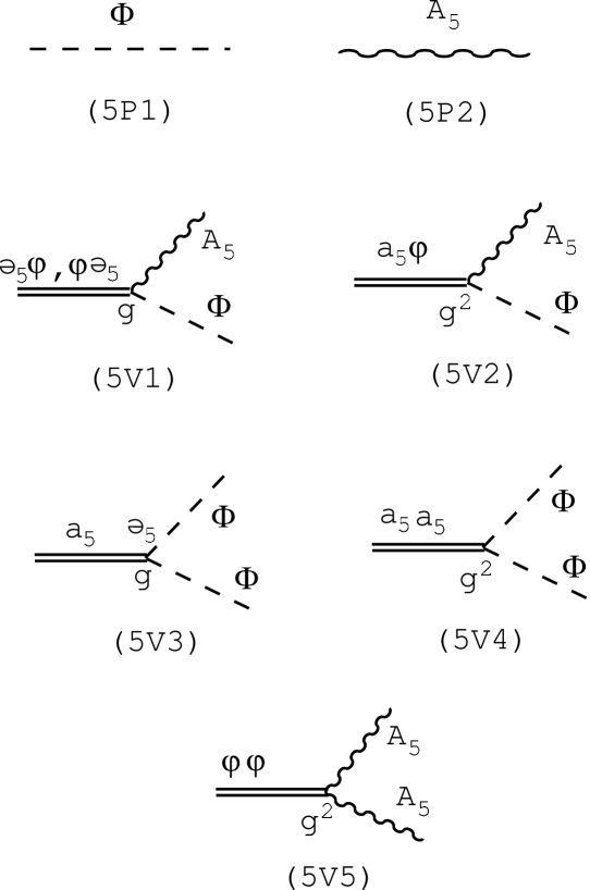
Figure 2: Feynman graphs for the bulk fields. (5P1),…(5V5) of (82).

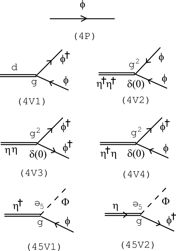
Figure 3: Feynman graphs for the boundary at ${x^{5}}=0$ and bulk-boundary-mixed fields. (4P),…(45V2) of (83). For all vertex graphs, the overall factor, $\delta({x^{5}})$, is omitted. See (83) for detail.

The corresponding terms in the Lagragian, from which the Feynman rules can be easily read, are given by, for the bulk part(Fig.2),

$$\mbox{(5P1)}\ :\ -{\frac{1}{2}}\partial_{M}\Phi_{\alpha}\partial^{M}\Phi_{\alpha}{\quad,}\quad\mbox{(5P2)}\ :\ -{\frac{1}{2}}\partial_{M}A_{5\alpha}\partial^{M}A_{5\alpha}{\quad,}$$

$$\mbox{(5V1)}\ :\ gf_{{\alpha\beta}\gamma}\{\partial_{5}\varphi_{\alpha}\cdot A_{5\beta}\Phi_{\gamma}+\partial_{5}\Phi_{\alpha}\cdot A_{5\beta}\varphi_{\gamma}\}{\quad,}$$

$$\mbox{(5V2)}\ :\ -g^{2}f_{{\alpha\beta}\tau}f_{\gamma\delta\tau}a_{5\alpha}\varphi_{\beta}A_{5\gamma}\Phi_{\delta}-g^{2}f_{{\alpha\beta}\tau}f_{\gamma\delta\tau}a_{5\alpha}\Phi_{\beta}A_{5\gamma}\varphi_{\delta}{\quad,}$$

$$\mbox{(5V3)}\ :\ gf_{{\alpha\beta}\gamma}\partial_{5}\Phi_{\alpha}a_{5\beta}\Phi_{\gamma}\ ,\ \mbox{(5V4)}\ :\ -\frac{g^{2}}{2}f_{{\alpha\beta}\tau}f_{\gamma\delta\tau}a_{5\alpha}\Phi_{\beta}a_{5\gamma}\Phi_{\delta}{\quad,}$$

$$\mbox{(5V5)}-\frac{g^{2}}{2}f_{{\alpha\beta}\tau}f_{\gamma\delta\tau}A_{5\alpha}\varphi_{\beta}A_{5\gamma}\varphi_{\delta}{\quad.}$$ (82)

They can be read from terms in ${\cal L}^{2}_{blk}|_{X^{3}=0}$ of (80). Those for the boundary at ${x^{5}}=0$ and mixed parts (Fig.3) are given by ”$\delta$-function parts” of (80).

$$\mbox{(4P)}\ :\ -\delta({x^{5}})\partial_{m}\phi^{\dagger}\partial^{m}\phi{\quad,}$$

$$\mbox{(4V1)}\ :\ \delta(x^{5})gd_{\alpha}\phi^{\dagger}T^{\alpha}\phi{\quad,}\quad\mbox{(4V2)}\ :\ -{\frac{1}{2}}g^{2}\delta(x^{5})\delta(0)(\eta^{\dagger}T^{\alpha}\phi)^{2}{\quad,}$$

$$\mbox{(4V3)}\ :\ -{\frac{1}{2}}g^{2}\delta(x^{5})\delta(0)(\phi^{\dagger}T^{\alpha}\eta)^{2}{\quad,}\quad$$

$$\mbox{(4V4)}\ :\ -g^{2}\delta(x^{5})\delta(0)(\eta^{\dagger}T^{\alpha}\phi)(\phi^{\dagger}T^{\alpha}\eta){\quad,}$$

$$\mbox{(45V1)}\ :\ -\delta(x^{5})g\partial_{5}\Phi_{\alpha}\eta^{\dagger}T^{\alpha}\phi{\quad,}\quad\mbox{(45V2)}\ :\ -\delta(x^{5})g\partial_{5}\Phi_{\alpha}\phi^{\dagger}T^{\alpha}\eta{\quad.}$$ (83)

Those for the boundary at ${x^{5}}=l$ and mixed parts are the same as above except the replacement: $\delta({x^{5}})\rightarrow\delta({x^{5}}-l),\phi\rightarrow\phi^{\prime},\eta\rightarrow\eta^{\prime}$.

(i) Boundary (4D) Quantum Effect

All divergent diagrams (for the chiral matter model) up to the order of $g^{3}$ are listed up in Fig.4. All are 1-loop diagrams within the ${x^{5}}=0$ brane.
The diagram (a) is interesting because its presence says Fayet-Iliopoulos D-term appears in the boundary due to the radiative correction. It is quadratically divergent. The term is proportional to ${\rm Tr\,}T^{\alpha}$, hence it exists only when the gauge group $G$ involves $U(1)$. If the appearance really happens it could give a dynamical SUSY breaking (see a textbook[24]). (Note that the tadpole diagram of massless field in 4D vanishes in the dimensional regularization [14] . Hence the presence of the FI D-term is rather subtle. ) This D-term does not appear in the vector-like matter case, ${\cal L}^{(b)}_{bnd}$, because the $\phi_{S}$ and $\phi_{R}$ contributions cancel each other. (The situation is the same as the super QED.)
The diagram (b) was considered in ref.[6]. It contributes, with (f) of Fig.5 explained later, to the self-energy of the scalar matter. This diagram (b) is independent of $d$, hence does not contribute to the effective potential under the SUSY boundary condition.
The diagram (c) gives the renormalization of D-field. The tree part is in the bulk as ${\rm tr\,}(X^{3}X^{3}-\partial_{5}\Phi\partial^{5}\Phi)$. (The corresponding part appears in Super QED. See $d^{2}$-term of eq.(210).)
The diagram (d) gives, with (g) of Fig.5, the renormalization of the gauge coupling $g$, and contributes to the $\beta$-function $\beta(g)$. (This part is very contrasting with the corresponding part of Super QED ($da{\bar{a}}$-term). We will discuss it in the final part of this section as (g)/Fig.5+(d)/Fig.4 part )

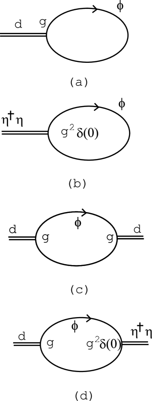
Figure 4: Divergent Feynman graphs for the boundary part up to the order of $g^{3}$.

The contribution to the effective potential of each diagram (of Fig.4) is given by

$$\mbox{(a) and (b)}\ :\ i\{gd_{\alpha}(T^{\alpha})_{{\beta^{\prime}}{\beta^{\prime}}}-g^{2}\delta(0)(\eta^{\dagger}T^{\alpha})_{\beta^{\prime}}(T^{\alpha}\eta)_{\beta^{\prime}}\}\int\frac{d^{4}k}{(2\pi)^{4}}\frac{1}{k^{2}}{\quad,}$$

$$\mbox{(c)}\ :\ \frac{i^{2}}{2!}g^{2}\cdot{\frac{1}{2}}d_{\alpha}d_{\alpha}\int\frac{d^{4}k}{(2\pi)^{4}}\frac{1}{(k^{2})^{2}}{\quad,}$$

$$\mbox{(d)}\ :\ \frac{i^{2}}{2!}\cdot 2\cdot(-g^{3}\delta(0))d_{\alpha}(\eta^{\dagger}T^{\beta}T^{\alpha}T^{\beta}\eta)\int\frac{d^{4}k}{(2\pi)^{4}}\frac{1}{(k^{2})^{2}}{\quad.}$$ (84)

(ii) Bulk (5D) Quantum Effect

Among bulk quantum propagations, we do not, at present, consider those which propagate between one brane and the other brane. Those diagrams play an important role as the gauge mediation mechanism in ref.[6]. The present interest, however, is not the SUSY breaking mechanism. This simplification is admitted because we can control the ignored contribution by adjusting the length $l$ between the two branes.

All divergent diagrams are listed up in Fig.5 up to the order of $g^{3}$. Only the diagram (g) contributes, others do not in the SUSY boundary condition. The diagram (f) was analysed in Ref.[6] for the calculation of the matter-field self energy. The diagram (g) gives the bulk contribution to the $\beta$-function of the coupling $g$.

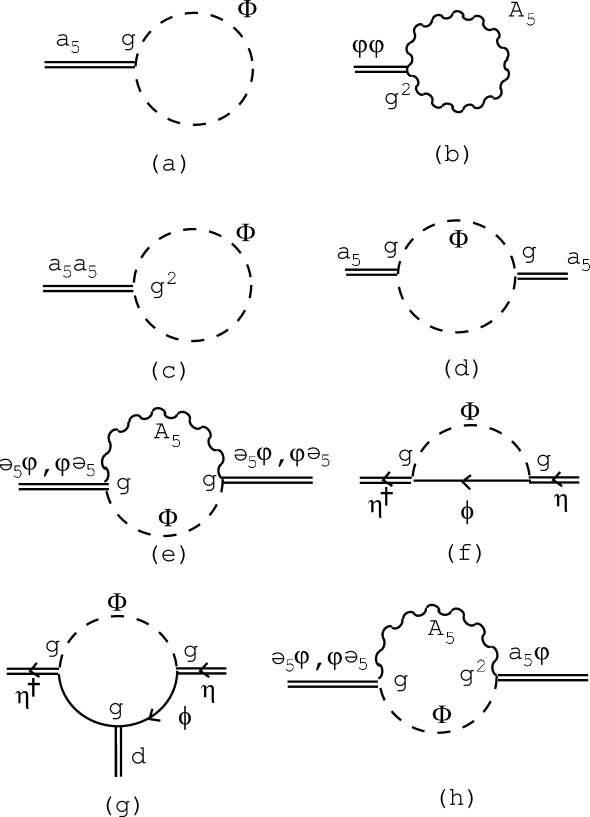
Figure 5: Divergent Feynman graphs for the bulk part up to the order of $g^{3}$.

The contribution to the effective potential of diagrams (f) and (g) are given by

$$\mbox{(f)}\ :\ g^{2}(\eta^{\dagger}T^{\alpha}T^{\alpha}\eta)\frac{i^{2}}{2!}\cdot 2\int_{k5}\frac{(k^{5})^{2}}{k^{2}+(k^{5})^{2}}\frac{1}{k^{2}}{\quad,}$$

$$\mbox{(g)}\ :\ g^{3}(\eta^{\dagger}T^{\alpha}T^{\gamma}T^{\alpha}\eta)d_{\gamma}(-1)\int_{k5}\frac{(k^{5})^{2}}{-k^{2}-(k^{5})^{2}}\frac{1}{(k^{2})^{2}}{\quad,}$$ (85)

where

$$\int_{k5}\equiv\int\frac{d^{4}k}{(2\pi)^{4}}\frac{1}{2l}\sum_{k^{5}\in{\frac{\pi}{l}}{\bf Z}}{\quad.}$$ (86)

The $k^{5}$-summation comes from the KK-expansion for the bulk field $\Phi$, which will be explained in (125). The result (f) of (85) is consistent with the corresponding term in (24) and (25) of ref.[6].

Using a formula

$$\sum_{n\in{\bf Z}}\frac{1}{x^{2}+n^{2}}=\frac{\pi}{x}\coth(\pi x){\quad,}$$ (87)

the $k^{5}$ summation part in (f) and (g) can be evaluated as ($k^{0}=ik^{4},k^{2}=(k^{1})^{2}+(k^{2})^{2}+(k^{3})^{2}+(k^{4})^{2}\equiv{\bar{k}}^{2}$)

$$\sum_{k^{5}\in{\frac{\pi}{l}}{\bf Z}}\frac{(k^{5})^{2}}{-k^{2}-(k^{5})^{2}}=-\sum_{k^{5}\in{\frac{\pi}{l}}{\bf Z}}\frac{(k^{5})^{2}}{{\bar{k}}^{2}+(k^{5})^{2}}$$

$$=-(\sum_{n\in{\bf Z}}1)+{\bar{k}}^{2}(\frac{l}{\pi})^{2}\sum_{n\in{\bf Z}}\frac{1}{{\bar{k}}^{2}(\frac{l}{\pi})^{2}+n^{2}}$$

$$=-2l\delta(0)+l\sqrt{{\bar{k}}^{2}}\coth(l\sqrt{{\bar{k}}^{2}}){\quad,}$$ (88)

where the Wick-rotation of $k^{0}$-axis is done and the relation

$$\sum_{n\in{\bf Z}}1=2l\delta(0){\quad,}$$ (89)

is used. The above result tells us the contribution from the singular parts in the boundary, that is, $\delta(0)$ parts in (b) and (d) of eq.(84)( see also Fig.4), cancel those in the bulk, that is, (f) and (g) of (85)( see also Fig.5). This phenomenon was pointed out for the self-energy diagrams in [6]. In App.B, it is shown that the cancellation phenomenon more generally (at the full order of the coupling within 1-loop) occurs in the effective potential. The final results are obtained as

$$\mbox{(f)/Fig.\ref{fig:BlkGraph}+(b)/Fig.\ref{fig:BndGraph}}\ :\ -g^{2}(\eta^{\dagger}T^{\alpha}T^{\alpha}\eta)\int\frac{id^{4}{\bar{k}}}{(2\pi)^{4}}{\frac{1}{2}}\sqrt{{\bar{k}}^{2}}\coth(l\sqrt{{\bar{k}}^{2}})\,\frac{1}{-{\bar{k}}^{2}}{\quad,}$$

$$\mbox{(g)/Fig.\ref{fig:BlkGraph}+(d)/Fig.\ref{fig:BndGraph}}\ :\ -g^{3}(\eta^{\dagger}T^{\alpha}T^{\gamma}T^{\alpha}\eta)d_{\gamma}\int\frac{id^{4}{\bar{k}}}{(2\pi)^{4}}{\frac{1}{2}}\sqrt{{\bar{k}}^{2}}\coth(l\sqrt{{\bar{k}}^{2}})\,\frac{1}{(-{\bar{k}}^{2})^{2}}{\quad.}$$ (90)

We note the above results give correct 4D expressions in the limit of $l\sqrt{{\bar{k}}^{2}}\ll 1$: $l\sqrt{{\bar{k}}^{2}}\coth(l\sqrt{{\bar{k}}^{2}})\rightarrow 1$. (See the $da{\bar{a}}$-part of Super QED, (210).) Hence the present bulk-boundary system can be regarded as some ”deformation” of the corresponding 4D theory.

If we write the main ”deformation” factor as follows

$$\coth(l\sqrt{{\bar{k}}^{2}})=1-2\sum_{n=0}^{\infty}{\rm e}^{-2nl\sqrt{{\bar{k}}^{2}}}{\quad,}$$ (91)

the role of the extra space becomes clear. Because the spectrum above ($"E_{n}"=n\sqrt{{\bar{k}}^{2}}$) shows that of the harmonic oscillator in the temperature $T=1/(2l)$, it can be translated as ”the whole (4D Euclidean) system is exposed to the heat-bath and in the equilibrium state with temperature $T=1/(2l)$”. The size of the extra space gives the inverse temperature. The $l\sqrt{{\bar{k}}^{2}}\ll 1$ limit in the previous paragraph corresponds to the high temperature limit.

Here the role of the singular term becomes clear. It is a ”counterterm” to cancel the divergences coming from the KK-mode summation. The (f)+(b) part is independent of $d$, hence it does not contribute to the SUSY effective potential. (We expect (f)+(b) part is cancelled by the vector- and spinor-loop contribution. ) This fact implies the above ”smoothing” phenomenon takes place independently of the SUSY requirement. We should note that, after the above cancellation, divergences, due to 4D-momentum integral, still remain. They correspond to the ordinary divergences due to the (SUSY) local interaction.

Let us obtain renormalization group quantities from the previous result, $\eta^{\dagger}T^{\gamma}\eta\,d_{\gamma}$-term. The ”deformed” propagator still makes the ultraviolet behaviour worse than the usual 4D propagator.

$$l\times\int\frac{d^{4}{\bar{k}}}{(2\pi)^{4}}\sqrt{{\bar{k}}^{2}}\coth(l\sqrt{{\bar{k}}^{2}})\frac{1}{({\bar{k}}^{2})^{2}}=\frac{1}{16\pi^{2}}\{l\Lambda-\ln 2-\ln\sinh l\epsilon\}{\quad,}$$ (92)

where $\Lambda$ and $\epsilon$ is the ultra-violet and infra-red cut-offs respectively, $\epsilon\leq|{\bar{k}}|\leq\Lambda$. (We do not care about the infra-red divergence because it can be cured by taking the massive matter multiplet.) It is linearly divergent. This result is reasonable from the power counting. Now we consider the scaling behaviour of the gauge coupling in the renormalization procedure. This problem is generally hard because the 5D gauge theory is regarded (perturbatively) nonrenormalizable. In the present case, however, we expect this model reduces to a 4D SUSY gauge theory in the limit $l\rightarrow 0$. We precisely define the limit as

$$\frac{g^{2}}{l}\equiv\alpha\quad(\mbox{fixed})\ll 1{\quad,}$$

$$l\rightarrow 0{\quad,}\quad g\rightarrow 0{\quad,}\quad g^{2}\ll l{\quad,}$$ (93)

where the dimensionless coupling $\alpha$ is introduced instead of $g^{2}$. From the relation $g^{2}\Lambda=\alpha\cdot l\Lambda$, we are naturally led to introduce another cut-off ${\tilde{\Lambda}}$ instead of $\Lambda$ as

$$l\Lambda\equiv\ln{\tilde{\Lambda}}{\quad.}$$ (94)

This relation connects two transformations, scaling and translation: ${\tilde{\Lambda}}\rightarrow{\tilde{\Lambda}}{\rm e}^{\nu}$(scaling) versus $\Lambda\rightarrow\Lambda+\nu/l$(translation). Then the renormalization group $\beta$-function of the dimensionless coupling $\alpha$ is obtained as

$$g_{b}=g+\Delta g=g(1+\frac{1}{8\times 16\pi^{2}}\alpha\ln{\tilde{\Lambda}}){\quad,}$$

$$\alpha_{b}=\frac{1}{l}(g+\Delta g)^{2}=\alpha(1+\frac{1}{4\times 16\pi^{2}}\alpha\ln{\tilde{\Lambda}}+O(\alpha^{2})){\quad,}$$

$$0=\frac{d}{d(\ln{\tilde{\Lambda}})}\ln\alpha_{b}=(1+O(\alpha))\frac{d}{d(\ln{\tilde{\Lambda}})}\ln\alpha+\frac{1}{4\times 16\pi^{2}}\alpha+O(\alpha^{2}){\quad,}$$

$$\beta_{\alpha}=\frac{d}{d(\ln{\tilde{\Lambda}})}\ln\alpha=-\frac{1}{4\times 16\pi^{2}}\alpha{\quad,}$$ (95)

where $g_{b}$ and $\alpha_{b}$ are bare quantities and G=SU(2) is taken ($T^{\alpha}T^{\gamma}T^{\alpha}=-T^{\gamma}/4$, see eq.(228)). The above result coincides with that of the ordinary 4D chiral-gauge SUSY theory (See textbooks[20, 26]). We confirm here that the correct 4D renormalization works although 5D quantum loop expression (92) is linearly divergent.

The previous paragraph confirms that the renormalization procedure works well at the 4D limit. In this paragraph, we argue a ”renormalization” procedure for the general case of $l$ (not limited to the $l\rightarrow 0$ case) and propose a practical approach to define a finite quantity from a divergent one ( such as (90), (92) ) coming from the 5D quantum effect. In the present standpoint the extra axis is regarded as a regularization axis. We have already pointed out that the macro parameter $1/l$ plays a role of the temperature $T=1/(2l)$ to smooth the UV behaviour. We recall a historically-famous fact in the beginning of the quantum mechanics. In the Planck distribution of the energy spectrum in a cavity, the light behaves like a wave in the high temperature region compared with its own energy (Rayleigh-Jeans’s region, $k_{B}T\geq h\nu$, where $k_{B}$ and $h$ are the Boltzman constant and the Planck constant respectively) whereas it behaves like a particle in the low temperature region (Wien’s region, $k_{B}T\leq h\nu$). In the present case, we are treating 5D quantum dynamics which can be regarded as a system composed of 4D Euclidean system of ”light” (oscillator) with energy $\sqrt{{\bar{k}}^{2}}$. They are thermally distributed in the heat-bath with the temperature $T=1/(2l)$. Now we take a natural restriction on the present treatment of the 5D quantum field theory: We cannot treat it in the Wien’s region because, in this region, ”the light” behaves like a particle and some new mass (energy) unit (probably the Planck mass) should exist in the theory. At present, however, we do not have such mass unit and it implies the present field theory treatment breaks down in the Wien’s region. (In other words, ”quantization” in the ”phase” space of $\Lambda$ and $l$ is lacking. ) We must switch to an unknown treatment in order to obtain a meaningful quantity from the divergent ones (90), (92). Let us propose a condition on the 4D momentum cut-off $\Lambda$. We should choose $\Lambda$ in such a way that the structure of the extra space (the circle in the present case) can not be recognized in the 4D world.

$$\Lambda\ \vbox{\kern 0.0pt\hbox{$<$}\hbox{$\sim$}}\ T=\frac{1}{2l}{\quad.}$$ (96)

If we adopt this idea , the integral (92) becomes well-defined( $l\Lambda\vbox{\kern 0.0pt\hbox{$<$}\hbox{$\sim$}}1$). Here we propose a sort of ”renormalization” for the present 5D quantum system. Note here that the UV cut-off $\Lambda$, of the 4D momentum ${\bar{k}}$, is essentially given by the inverse of the IR cut-off parameter $l$ of the extra space. In this way, we have the following relation

$$|{\bar{k}}|\leq\Lambda\vbox{\kern 0.0pt\hbox{$<$}\hbox{$\sim$}}\frac{1}{2l}=T{\quad.}$$ (97)

This is a sort of ”mass hierarchy” relation which appears in extra-dimensional models. The relation (97) reminds us of the similar one that appears in the regularization of fermion determinant (the domain wall fermion or the overlap formalism) in the lattice field theory. (See (32) of ref.[30], eq.(29) of ref.[31], and eq.(26) of ref.[32].) The chiral symmetry in the fermion system corresponds to $Z^{2}$-symmetry in the present case.

In this section, we have confirmed that the renormalization works well as far as the 4D world is concerned. Aside from the (5D) renormalization problem, we next examine the vacuum structure.

6 Vacuum in the Brane World and Mass Matrix

First we examine the vacuum in the present 5D approach. The relevant scalars are $a_{5}$ and $\varphi$, that is, the background fields of $A_{5}$ (the extra component of the bulk vector) and $\Phi$ (the bulk scalar) respectively. They should be, in principle, given by solving the (renormalized) equation of motion. They describe the vacuum. We usually take the following procedure in order to obtain a vacuum.

[Ordinary procedure for the vacuum search[33]]
1) First we obtain the effective potential assuming the scalar property of the vacuum (as described in (68,70)) and the constancy of the scalar vacuum expectation values.
2) Take the minimum of the effective potential.

At the present case, however, we should take into account the $x^{5}$-dependency and the Z₂-property of the vacuum expectation value. We take the following forms of $a_{5}({x^{5}})$ and $\varphi({x^{5}})$, which describe the localized (around $x^{5}=0,l$) configuration and a natural generalization of the ordinary treatment stated above.

$$a_{5\gamma}({x^{5}})={\bar{a}}_{\gamma}\,\epsilon({x^{5}}){\quad,}\quad\varphi_{\gamma}({x^{5}})={\bar{\varphi}}_{\gamma}\epsilon({x^{5}}){\quad,}$$

$$\epsilon({x^{5}})=\left\{\begin{array}[]{cc}+1&\mbox{for }2nl<{x^{5}}<(1+2n)l\\ 0&\mbox{for }{x^{5}}=nl\\ -1&\mbox{for }(2n-1)l<{x^{5}}<2nl\end{array}\right.\quad n\in{\bf Z}{\quad,}$$ (101)

where $\epsilon({x^{5}})$ is the periodic sign function with the periodicity $2l$. ${\bar{a}}_{\gamma}$ and ${\bar{\varphi}}_{\gamma}$ are positive constants. See Fig.6 and Fig.7.

Figure 6: Behaviour of the background field $a_{5\gamma}(x^{5})$ (the extra component of the bulk vector).

Figure 7: Behaviour of the background field $\varphi_{\gamma}(x^{5})$(the bulk scalar).

It is shown, in App.C, that the above forms of $a_{5}({x^{5}})$ and $\varphi({x^{5}})$ satisfy the field equation of the present model. The periodic sign function can be regarded as the thin-wall limit of a kink solution and shows the localization of the bulk scalar and the extra component of the bulk vector. This generalization is also natural from the viewpoint that the present theory starts with the singular interaction ($\delta$-function term of (44).). We may use the piecewise-continuous or piecewise-smooth functions as the theoretical materials, which is required from Z₂-property[35].

We now begin to prepare for the full ( with respect to the coupling order) calculation of the 1-loop effective potential. The ”1-loop” action, (80), can be expressed as

$$S^{2}_{a}=S^{free}_{a}+S^{ghost}+\int d^{5}X$$

$$\times{\frac{1}{2}}\left(\begin{array}[]{cccc}\phi^{\dagger}_{\alpha^{\prime}}&\phi_{\alpha^{\prime}}&\Phi_{\alpha}&A_{5\alpha}\end{array}\right){\left(\begin{array}[]{cc}\left(\begin{array}[]{cc}M_{\phi^{\dagger}\phi}&M_{\phi^{\dagger}\phi^{\dagger}}\\ M_{\phi\phi}&M_{\phi\phi^{\dagger}}\\ \end{array}\right)_{{\alpha^{\prime}}{\beta^{\prime}}}&\left(\begin{array}[]{cc}M_{\phi^{\dagger}\Phi}&0\\ M_{\phi\Phi}&0\end{array}\right)_{{\alpha^{\prime}}\beta}\\ \left(\begin{array}[]{cc}M_{\Phi\phi}&M_{\Phi\phi^{\dagger}}\\ 0&0\end{array}\right)_{\alpha{\beta^{\prime}}}&\left(\begin{array}[]{cc}M_{\Phi\Phi}&M_{\Phi A_{5}}\\ M_{A_{5}\Phi}&M_{A_{5}A_{5}}\end{array}\right)_{\alpha\beta}\end{array}\right)}\left(\begin{array}[]{c}\phi_{\beta^{\prime}}\\ \phi^{\dagger}_{\beta^{\prime}}\\ \Phi_{\beta}\\ A_{5\beta}\end{array}\right)$$ (117)

$$+(\phi^{\prime}\mbox{ and }\phi^{{}^{\prime}{\dagger}}\mbox{involving terms}),$$

$$S^{free}_{a}={\int d^{5}X}\left[{\rm tr\,}\,\{-\partial_{M}\Phi\partial^{M}\Phi-\partial_{M}A_{5}\partial^{M}A_{5}\}-\delta({x^{5}})\partial_{m}\phi^{\dagger}\partial^{m}\phi\right],$$

$$S^{ghost}=-\int d^{5}X\left[\partial_{M}{\bar{c}}_{\alpha}\cdot\partial^{M}c_{\alpha}+igf_{{\alpha\beta}\gamma}\partial_{5}{\bar{c}}_{\alpha}\cdot a_{5\beta}c_{\gamma}\right]{\quad,}$$ (118)

where each component is read from (80) as

$$(M_{\phi^{\dagger}\phi})_{{\alpha^{\prime}}{\beta^{\prime}}}=g\delta({x^{5}})d_{\gamma}(T^{\gamma})_{{\alpha^{\prime}}{\beta^{\prime}}}-g^{2}\delta(0)\delta({x^{5}})(T^{\gamma}\eta)_{\alpha^{\prime}}(\eta^{\dagger}T^{\gamma})_{\beta^{\prime}}{\quad,}$$

$$(M_{\phi\phi^{\dagger}})_{{\alpha^{\prime}}{\beta^{\prime}}}=g\delta({x^{5}})d_{\gamma}(T^{\gamma})_{{\beta^{\prime}}{\alpha^{\prime}}}-g^{2}\delta(0)\delta({x^{5}})(\eta^{\dagger}T^{\gamma})_{\alpha^{\prime}}(T^{\gamma}\eta)_{\beta^{\prime}}{\quad,}$$

$$(M_{\phi\phi})_{{\alpha^{\prime}}{\beta^{\prime}}}=-g^{2}\delta(0)\delta({x^{5}})(\eta^{\dagger}T^{\gamma})_{\alpha^{\prime}}(\eta^{\dagger}T^{\gamma})_{\beta^{\prime}}$$

$$(M_{\phi^{\dagger}\phi^{\dagger}})_{{\alpha^{\prime}}{\beta^{\prime}}}=-g^{2}\delta(0)\delta({x^{5}})(T^{\gamma}\eta)_{\alpha^{\prime}}(T^{\gamma}\eta)_{\beta^{\prime}}\ ,$$

$$(M_{\Phi\phi})_{\alpha{\beta^{\prime}}}=(M_{\phi\Phi})_{{\beta^{\prime}}\alpha}=g\partial_{5}\delta({x^{5}})\cdot(\eta^{\dagger}T^{\alpha})_{\beta^{\prime}}\ ,$$

$$(M_{\Phi\phi^{\dagger}})_{\alpha{\beta^{\prime}}}=(M_{\phi^{\dagger}\Phi})_{{\beta^{\prime}}\alpha}=g\partial_{5}\delta({x^{5}})\cdot(T^{\alpha}\eta)_{\beta^{\prime}}\ ,$$

$$(M_{\Phi\Phi})_{\alpha\beta}=-g{\vbox{\halign{#\cr$\leftarrow$\crcr\kern-1.0pt\nointerlineskip\cr$\hfil\displaystyle{\partial}\hfil$\crcr}}}_{5}f_{{\alpha\beta}\gamma}a_{5\gamma}+gf_{{\alpha\beta}\gamma}a_{5\gamma}{\vec{\partial}}_{5}-g^{2}f_{\alpha\delta\tau}f_{\beta\gamma\tau}a_{5\delta}a_{5\gamma}\ ,$$ (121)

$$(M_{A_{5}A_{5}})_{\alpha\beta}=-g^{2}f_{\alpha\gamma\tau}f_{\beta\delta\tau}\varphi_{\gamma}\varphi_{\delta}\ ,$$

$$(M_{A_{5}\Phi})_{\alpha\beta}=gf_{{\alpha\beta}\gamma}\partial_{5}\varphi_{\gamma}-gf_{{\alpha\beta}\gamma}\varphi_{\gamma}{\vec{\partial}}_{5}-g^{2}f_{{\alpha\beta}\tau}f_{\gamma\delta\tau}a_{5\gamma}\varphi_{\delta}-g^{2}f_{\gamma\beta\tau}f_{\alpha\delta\tau}a_{5\gamma}\varphi_{\delta}\ ,$$

$$(M_{\Phi A_{5}})_{\alpha\beta}=-gf_{{\alpha\beta}\gamma}\partial_{5}\varphi_{\gamma}+gf_{{\alpha\beta}\gamma}{\vbox{\halign{#\cr$\leftarrow$\crcr\kern-1.0pt\nointerlineskip\cr$\hfil\displaystyle{\partial}\hfil$\crcr}}}_{5}\varphi_{\gamma}+g^{2}f_{{\alpha\beta}\tau}f_{\gamma\delta\tau}a_{5\gamma}\varphi_{\delta}-g^{2}f_{\gamma\alpha\tau}f_{\beta\delta\tau}a_{5\gamma}\varphi_{\delta}{\quad.}$$ (124)

In the present analysis, as mentioned in Sect.5, we ignore the quantum propagation between the two branes. We consider only the case that the quantum-loops propagate between the ${x^{5}}=0$ brane and the bulk or purely within the ${x^{5}}=0$ brane. Hence we may ignore the $\delta({x^{5}}-l)$-terms in the above expression.

From the periodicity (${x^{5}}\rightarrow{x^{5}}+2l$) and the Z₂-odd property, the bulk fields $\Phi(X),A_{5}(X)$ can be KK-expanded as

$$\Phi(x,{x^{5}})=\frac{1}{\sqrt{l}}\sum_{n=1}^{\infty}\Phi_{n}(x)\sin({\frac{n\pi}{l}}{x^{5}}){\quad,}$$

$$A_{5}(x,{x^{5}})=\frac{1}{\sqrt{l}}\sum_{n=1}^{\infty}A_{n}(x)\sin({\frac{n\pi}{l}}{x^{5}}){\quad,}$$ (125)

where the normalization is taken in the way: $\int_{-l}^{l}\Phi^{2}d{x^{5}}=\sum_{n=1}^{\infty}{\Phi_{n}(x)}^{2},\ \int_{-l}^{l}{A_{5}}^{2}d{x^{5}}=\sum_{n=1}^{\infty}{A_{n}(x)}^{2}.$

We evaluate the action term by term.

(i) Free Part of the bulk and boundary system

The free part $S^{free}_{a}$ can be obtained as

$$S^{free}_{a}=\int d^{4}x$$

$$\left[\sum_{k=1}^{\infty}{\rm tr\,}\left\{-\partial_{m}\Phi_{k}\partial^{m}\Phi_{k}-(\frac{k\pi}{l})^{2}\Phi_{k}^{2}-\partial_{m}A_{k}\partial^{m}A_{k}-(\frac{k\pi}{l})^{2}A_{k}^{2}\right\}-\partial_{m}\phi^{\dagger}\partial^{m}\phi\right]\ .$$ (126)

From the Z₂-odd property, zero KK-mode does not appear. All quantum modes are massive with the order of $l^{-1}$.

(ii) $M_{\phi^{\dagger}\phi},M_{\phi^{\dagger}\phi^{\dagger}},M_{\phi\phi},M_{\phi\phi^{\dagger}}$ (boundary part)

The boundary part can be read from (124).

(iii)$M_{\phi^{\dagger}\Phi},M_{\phi\Phi},M_{\Phi\phi},M_{\Phi\phi^{\dagger}}$ (bulk-boundary mixed part)

$${\frac{1}{2}}{\int d^{5}X}\phi_{\alpha^{\prime}}(M_{\phi\Phi})_{{\alpha^{\prime}}\beta}\Phi_{\beta}={\frac{1}{2}}{\int d^{5}X}\Phi_{\alpha}(M_{\Phi\phi})_{\alpha{\beta^{\prime}}}\phi_{\beta^{\prime}}=$$

$$-\frac{g}{2\sqrt{l}}{\int d^{4}x}(\eta^{\dagger}T^{\beta}\phi)\sum_{n=1}^{\infty}{\frac{n\pi}{l}}\Phi_{n\beta}(x){\quad,}$$

$${\frac{1}{2}}{\int d^{5}X}\phi^{\dagger}_{\alpha^{\prime}}(M_{\phi^{\dagger}\Phi})_{{\alpha^{\prime}}\beta}\Phi_{\beta}={\frac{1}{2}}{\int d^{5}X}\Phi_{\alpha}(M_{\Phi\phi^{\dagger}})_{\alpha{\beta^{\prime}}}\phi^{\dagger}_{\beta^{\prime}}=$$

$$-\frac{g}{2\sqrt{l}}{\int d^{4}x}(\phi^{\dagger}T^{\alpha}\eta)\sum_{n=1}^{\infty}{\frac{n\pi}{l}}\Phi_{n\alpha}(x){\quad.}$$ (127)

The remaining ones are bulk-bulk contribution.

(iv)$M_{\Phi\Phi}$
The one part of ${\frac{1}{2}}{\int d^{5}X}\,\Phi_{\alpha}(M_{\Phi\Phi})_{\alpha\beta}\Phi_{\beta}\equiv S^{int}_{iv}$ is evaluated as

$$S^{int}_{iv1}\equiv\frac{-g^{2}}{2}{\int d^{5}X}f_{\alpha\delta\tau}f_{\beta\gamma\tau}a_{5\delta}a_{5\gamma}\Phi_{\alpha}\Phi_{\beta}$$

$$=-\frac{g^{2}}{2}f_{\alpha\delta\tau}f_{\beta\gamma\tau}{\bar{a}}_{\delta}{\bar{a}}_{\gamma}{\int d^{4}x}\sum_{n=1}^{\infty}\Phi_{n\alpha}(x)\Phi_{n\beta}(x){\quad,}$$ (128)

where we use $a_{5\delta}a_{5\gamma}={\bar{a}}_{5\delta}{\bar{a}}_{5\gamma}\epsilon({x^{5}})^{2}={\bar{a}}_{5\delta}{\bar{a}}_{5\gamma}$. The other part can be expressed as

$$S^{int}_{iv2}\equiv\frac{g}{2}{\int d^{5}X}f_{{\alpha\beta}\gamma}a_{5\gamma}(-\partial_{5}\Phi_{\alpha}\,\Phi_{\beta}+\Phi_{\alpha}\partial_{5}\Phi_{\beta})$$

$$=-gf_{{\alpha\beta}\gamma}{\bar{a}}_{\gamma}{\int d^{4}x}\int_{-l}^{l}d{x^{5}}\epsilon({x^{5}})\partial_{5}\Phi_{\alpha}\cdot\Phi_{\beta}{\quad.}$$ (129)

Using the Fourier expansion of the periodic sign function,

$$\epsilon(x)=\frac{4}{\pi}\sum_{n=0}^{\infty}\frac{1}{2n+1}\sin\{\frac{(2n+1)\pi}{l}x\}{\quad,}$$ (130)

we obtain

$$S^{int}_{iv2}=\frac{2g}{l}f_{{\alpha\beta}\gamma}{\bar{a}}_{\gamma}{\int d^{4}x}\sum_{m=1}^{\infty}\sum_{n=1}^{\infty}\Phi_{m\alpha}mQ_{mn}\Phi_{n\beta}{\quad,}$$

$$\int_{-l}^{l}d{x^{5}}\epsilon({x^{5}})\cos({\frac{m\pi}{l}}{x^{5}})\sin({\frac{n\pi}{l}}{x^{5}})=-\frac{2l}{\pi}Q_{mn}{\quad,}$$

$$Q_{mn}=\left\{\begin{array}[]{cc}\frac{1}{m-n}&m-n=\mbox{odd}\\ 0&m-n=\mbox{even}\end{array}\right.=\left\{\begin{array}[]{cc}{\frac{1}{2}}\{1-(-1)^{m-n}\}\frac{1}{m-n}&m\neq n\\ 0&m=n\end{array}\right.{\quad.}$$ (135)

We note the anti-symmetricity: $Q_{mn}=-Q_{nm}$.

(v)$M_{A_{5}A_{5}}$

$$S^{int}_{v}\equiv{\frac{1}{2}}{\int d^{5}X}A_{5\alpha}(X)(M_{A_{5}A_{5}})_{\alpha\beta}A_{5\beta}(X)$$

$$=-\frac{g^{2}}{2l}f_{\alpha\gamma\tau}f_{\beta\delta\tau}\sum_{n=1}^{\infty}\sum_{k=1}^{\infty}{\int d^{4}x}A_{n\alpha}(x)A_{k\beta}(x)\times$$

$$\int_{-l}^{l}d{x^{5}}\,\varphi_{\gamma}({x^{5}})\varphi_{\delta}({x^{5}})\sin({\frac{n\pi}{l}}{x^{5}})\sin({\frac{k\pi}{l}}{x^{5}}){\quad.}$$ (136)

Using the localized form of $\varphi({x^{5}})$ given in (101), we obtain

$$S^{int}_{v}=-\frac{g^{2}}{2}f_{\alpha\gamma\tau}f_{\beta\delta\tau}\,\sum_{n=1}^{\infty}{\bar{\varphi}}_{\gamma}{\bar{\varphi}}_{\delta}{\int d^{4}x}A_{n\alpha}(x)A_{n\beta}(x){\quad.}$$ (137)

(vi)$M_{\Phi A_{5}},M_{A_{5}\Phi}$

This group consists of four terms.

$$S^{int}_{vi}\equiv{\frac{1}{2}}{\int d^{5}X}\Phi_{\alpha}(M_{\Phi A_{5}})_{\alpha\beta}A_{5\beta}={\frac{1}{2}}{\int d^{5}X}A_{5\alpha}(M_{A_{5}\Phi})_{\alpha\beta}\Phi_{\beta}$$

$$=S^{int}_{vi1}+S^{int}_{vi2}+S^{int}_{vi3}+S^{int}_{vi4}{\quad,}$$

$$S^{int}_{vi1}=-{\frac{1}{2}}{\int d^{5}X}gf_{{\alpha\beta}\gamma}\Phi_{\alpha}\partial_{5}\varphi_{\gamma}\,A_{5\beta}\ ,\ S^{int}_{vi2}={\frac{1}{2}}{\int d^{5}X}gf_{{\alpha\beta}\gamma}\partial_{5}\Phi_{\alpha}\,\varphi_{\gamma}A_{5\beta}\ ,$$

$$S^{int}_{vi3}={\frac{1}{2}}{\int d^{5}X}g^{2}f_{{\alpha\beta}\tau}f_{\gamma\delta\tau}\Phi_{\alpha}a_{5\gamma}\varphi_{\delta}A_{5\beta}\ ,\ S^{int}_{vi4}=-{\frac{1}{2}}{\int d^{5}X}g^{2}f_{\gamma\alpha\tau}f_{\beta\delta\tau}\Phi_{\alpha}a_{5\gamma}\varphi_{\delta}A_{5\beta}\ .$$ (138)

Here we note the relation

$$\partial_{5}\varphi_{\gamma}=2{\bar{\varphi}}_{\gamma}\{\delta({x^{5}})-\delta({x^{5}}-l)\}{\quad,}$$ (139)

which expresses the localization of the bulk scalar. $\delta(x)$ is the periodic (periodicity $2l$) delta function. See Fig.8.

Figure 8: Behaviour of $\partial_{5}\varphi_{\gamma}(x^{5})$.

Using the above equation, we can evaluate the first term as follows.

$$S^{int}_{vi1}=-gf_{{\alpha\beta}\gamma}{\bar{\varphi}}_{\gamma}{\int d^{4}x}\left[\left.\Phi_{\alpha}A_{5\beta}\right|_{{x^{5}}=0}-\left.\Phi_{\alpha}A_{5\beta}\right|_{{x^{5}}=l}\right]=0{\quad.}$$ (140)

The third and fourth terms are evaluated as

$$S^{int}_{vi3}=\frac{g^{2}}{2}f_{{\alpha\beta}\tau}f_{\gamma\delta\tau}{\bar{a}}_{\gamma}{\bar{\varphi}}_{\delta}\sum_{n=1}^{\infty}{\int d^{4}x}\,\Phi_{n\alpha}(x)A_{n\beta}(x){\quad,}$$

$$S^{int}_{vi4}=-\frac{g^{2}}{2}f_{\gamma\alpha\tau}f_{\beta\delta\tau}{\bar{a}}_{\gamma}{\bar{\varphi}}_{\delta}\sum_{n=1}^{\infty}{\int d^{4}x}\,\Phi_{n\alpha}(x)A_{n\beta}(x){\quad.}$$ (141)

Using the relation (135), we obtain

$$S^{int}_{vi2}=-\frac{g}{l}f_{{\alpha\beta}\gamma}{\bar{\varphi}}_{\gamma}\sum_{m=1}^{\infty}\sum_{n=1}^{\infty}\Phi_{m\alpha}mQ_{mn}A_{n\beta}{\quad.}$$ (142)

The background fields we take, (101), satisfy the required boundary condition. They also satisfy the on-shell condition (76) for an appropriate choice of ${\bar{a}},{\bar{\varphi}},\eta,\eta^{\dagger}$ and $\chi^{3}$. Explanation is given in App.C.

We summarize the results of (i)-(vi) as follows.

$$S^{2}_{a}=S^{ghost}+\int d^{4}x\times$$

$${\frac{1}{2}}\left(\begin{array}[]{cccc}\phi^{\dagger}_{\alpha^{\prime}}&\phi_{\alpha^{\prime}}&\Phi_{m\alpha}&A_{m\alpha}\end{array}\right){\left(\begin{array}[]{cc}\left(\begin{array}[]{cc}{\cal M}_{\phi^{\dagger}\phi}&{\cal M}_{\phi^{\dagger}\phi^{\dagger}}\\ {\cal M}_{\phi\phi}&{\cal M}_{\phi\phi^{\dagger}}\\ \end{array}\right)_{{\alpha^{\prime}}\,{\beta^{\prime}}}&\left(\begin{array}[]{cc}{\cal M}_{\phi^{\dagger}\Phi}&0\\ {\cal M}_{\phi\Phi}&0\end{array}\right)_{{\alpha^{\prime}}\,n\beta}\\ \left(\begin{array}[]{cc}{\cal M}_{\Phi\phi}&{\cal M}_{\Phi\phi^{\dagger}}\\ 0&0\end{array}\right)_{m\alpha\,{\beta^{\prime}}}&\left(\begin{array}[]{cc}{\cal M}_{\Phi\Phi}&{\cal M}_{\Phi A}\\ {\cal M}_{A\Phi}&{\cal M}_{AA}\end{array}\right)_{m\alpha\,n\beta}\end{array}\right)}\left(\begin{array}[]{c}\phi_{\beta^{\prime}}\\ \phi^{\dagger}_{\beta^{\prime}}\\ \Phi_{n\beta}\\ A_{n\beta}\end{array}\right)$$ (158)

$$+(\phi^{\prime}\mbox{ and }\phi^{{}^{\prime}{\dagger}}\mbox{involving terms}){\quad,}$$ (159)

where the integer suffixes $m$ and $n$ runs from 1 to $\infty$, and each component is described as

$${\cal M}_{\phi^{\dagger}_{\alpha^{\prime}}\phi_{\beta^{\prime}}}=\partial^{2}\delta_{{\alpha^{\prime}}{\beta^{\prime}}}+gd_{\gamma}(T^{\gamma})_{{\alpha^{\prime}}{\beta^{\prime}}}-g^{2}\delta(0)(T^{\gamma}\eta)_{\alpha^{\prime}}(\eta^{\dagger}T^{\gamma})_{\beta^{\prime}}{\quad,}$$

$${\cal M}_{\phi^{\dagger}_{\alpha^{\prime}}\phi^{\dagger}_{\beta^{\prime}}}=-g^{2}\delta(0)(T^{\gamma}\eta)_{\alpha^{\prime}}(T^{\gamma}\eta)_{\beta^{\prime}}{\quad,}\quad{\cal M}_{\phi_{\alpha^{\prime}}\phi_{\beta^{\prime}}}=-g^{2}\delta(0)(\eta^{\dagger}T^{\gamma})_{\alpha^{\prime}}(\eta^{\dagger}T^{\gamma})_{\beta^{\prime}}{\quad,}$$

$${\cal M}_{\phi_{\alpha^{\prime}}\phi^{\dagger}_{\beta^{\prime}}}=\partial^{2}\delta_{{\alpha^{\prime}}{\beta^{\prime}}}+gd_{\gamma}(T^{\gamma})_{{\beta^{\prime}}{\alpha^{\prime}}}-g^{2}\delta(0)(\eta^{\dagger}T^{\gamma})_{\alpha^{\prime}}(T^{\gamma}\eta)_{\beta^{\prime}}$$

$${\cal M}_{\phi^{\dagger}_{\alpha^{\prime}}\Phi_{n\beta}}=-\frac{g}{\sqrt{l}}(T^{\beta}\eta)_{\alpha^{\prime}}{\frac{n\pi}{l}}={\cal M}_{\Phi_{n\beta}\phi^{\dagger}_{\alpha^{\prime}}}{\quad,}\quad{\cal M}_{\phi_{\alpha^{\prime}}\Phi_{n\beta}}=-\frac{g}{\sqrt{l}}(\eta^{\dagger}T^{\beta})_{\alpha^{\prime}}{\frac{n\pi}{l}}={\cal M}_{\Phi_{n\beta}\phi_{\alpha^{\prime}}}{\quad,}$$

$${\cal M}_{\Phi_{m\alpha}\Phi_{n\beta}}=-\{-\partial^{2}+({\frac{n\pi}{l}})^{2}\}\delta_{mn}\delta_{\alpha\beta}-g^{2}f_{\alpha\delta\tau}f_{\beta\gamma\tau}{\bar{a}}_{\delta}{\bar{a}}_{\gamma}\delta_{mn}+\frac{4g}{l}f_{{\alpha\beta}\gamma}{\bar{a}}_{\gamma}mQ_{mn}{\quad,}$$

$${\cal M}_{\Phi_{m\alpha}A_{n\beta}}=g^{2}f_{{\alpha\beta}\tau}f_{\gamma\delta\tau}{\bar{a}}_{\gamma}{\bar{\varphi}}_{\delta}\delta_{mn}-g^{2}f_{\gamma\alpha\tau}f_{\beta\delta\tau}{\bar{a}}_{\gamma}{\bar{\varphi}}_{\delta}\delta_{mn}-\frac{2g}{l}f_{{\alpha\beta}\gamma}{\bar{\varphi}}_{\gamma}mQ_{mn}={\cal M}_{A_{n\beta}\Phi_{m\alpha}},$$

$${\cal M}_{A_{m\alpha}A_{n\beta}}=-\{-\partial^{2}+({\frac{n\pi}{l}})^{2}\}\delta_{mn}\delta_{\alpha\beta}-g^{2}f_{\alpha\gamma\tau}f_{\beta\delta\tau}{\bar{\varphi}}_{\gamma}{\bar{\varphi}}_{\delta}\delta_{mn}{\quad.}$$ (160)

where the kinetic (free) part, $S^{free}_{a}$, is included ($\partial^{2}\equiv\partial_{m}\partial^{m}$ is the 4D Laplacian) in the “Mass” matrix. The repeated indices imply the Einstein’s summation convention.

7 Effective Potential of Bulk-Boundary System

As shown in Sec.2 and App.A for simple models, the effective potential is obtained from the eigenvalues of the relevant mass-matrix obtained by the background expansion. Let us obtain the effective potential from the mass matrix ${\cal M}$ of (159) and (160). It is composed of three field values $\eta,\eta^{\dagger},d_{\alpha}$, two wall ”heights”, ${\bar{a}}_{\alpha},{\bar{\varphi}}_{\alpha}$, the gauge coupling, $g$ and the boundary parameter $l$. The full explicit calculation, even at 1-loop level, is technically hard. We obtain some interesting ”sections” of the full result: Case (A), $\eta=0,\eta^{\dagger}=0$; Case (B), ${\bar{a}}=0,{\bar{\varphi}}=0$. Detailed explanation is given in App.B.

Case (A): $\eta=0,\eta^{\dagger}=0$
We look the potential with the suppression of the scalar matter dependence. (Or we may say we look the potential from the $\eta=\eta^{\dagger}=0$ point. ) In this case the mass matrix ${\cal M}$ has the following properties:  (1) In ${\cal M}$, the boundary part and the bulk one decouple each other;  (2) All $\delta(0)$-terms disappear. The boundary-loop quantum effect gives rise to the following potential before the renormalization procedure:

$$V^{eff}_{1-loop}=\int\frac{d^{4}k}{(2\pi)^{4}}\ln\{1-\frac{g^{2}}{4}\frac{d^{2}}{(k^{2})^{2}}\}{\quad,}$$ (161)

where we take G=SU(2) as the internal gauge group. The behaviour is similar to the super QED explained in App.A. The above expression, when treated perturbatively, is logarithmically divergent. Noting the relation: $d_{\alpha}=(\chi^{3}-\partial_{5}\varphi+ga_{5}\times\varphi)_{\alpha},$ we realize the renormalization procedure connects the boundary and the bulk phenomena through the field renormalization of $X^{3}$ and $\Phi$ although we do not touch on the renormalization of the bulk fields.

The bulk-loop quantum effect does not give the $d_{\alpha}$-dependence to the vacuum energy. Hence it does not contribute to the effective potential after the use of the SUSY boundary condition. It gives, however, an important result:  the scalar-loop contribution to the vacuum energy which depends on the ”wall heights” ${\bar{a}}$ and ${\bar{\varphi}}$. (We expect some part of the contribution appear when the boson-fermion balance breaks down due to some SUSY breaking mechanism. ) We can regard it as a new type Casimir energy, because ${\bar{a}}$ and ${\bar{\varphi}}$ can be regarded as different-type boundary parameters from $l$.[36] For the large circle limit $l\rightarrow\infty$, the final result of the new Casimir energy, per one KK-mode, is

$$\frac{1}{l}V^{eff}_{Casimir}=\frac{g^{2}}{l^{3}}(\alpha_{1}{\bar{\varphi}}^{2}+\alpha_{2}{\bar{a}}^{2}+\alpha_{3}{\bar{a}}\cdot{\bar{\varphi}})+O(g^{4}){\quad,}$$ (162)

where $\alpha_{1},\alpha_{2}$ and $\alpha_{3}$ are some constants. The new points, compared with the ordinary Casimir energy[7], are 1) the potential depends on the circle radius as $l^{-3}$; 2) the potential depends on the gauge coupling $g$; 3) the potential depends on the ”wall heights”, ${\bar{\varphi}}$ and ${\bar{a}}$. We expect the above quantity (162) does not depend on the gauge we have chosen [37]. This contribution from the scalar loop, however, is expected to be cancelled by those from the fermion and vector loops in the present SUSY-invariant setting.

Case (B): ${\bar{a}}=0,{\bar{\varphi}}=0$
In this case the brane structure disappears. The situation is similar to the case of Appelquist and Chodos(AC). From the bulk modes of $\Phi$ and $A_{5}$, we have AC-type eigenvalues.

$$\lambda_{n}=-k^{2}-({\frac{n\pi}{l}})^{2}{\quad,}\quad n=1,2,3,\cdots{\quad,}$$ (163)

(See (309) and (404)). This gives the famous form of the Casimir energy.

$$\frac{1}{l}V^{eff}_{Casimir}=\frac{\mbox{const}}{l^{5}}{\quad.}$$ (164)

This is the scalar-loop contribution and is expected to be cancelled by other non-scalar fields effect.

The eigenvalues for the boundary part is obtained as a complicated expression involving the following terms:

$$S\equiv\eta^{\dagger}\eta\ ,\ d^{2}=d_{\alpha}d_{\alpha}\ ,\ d\cdot V\equiv d_{\alpha}\,\eta^{\dagger}T^{\alpha}\eta\ ,\ V^{2}\equiv(\eta^{\dagger}T^{\alpha}\eta)^{2}{\quad.}$$ (165)

We have the full expression in the computer file. In the manipulation of eigenvalues search (determinant calculation), we face the following combination of terms.

$$\delta(0)+\frac{1}{l}\sum_{m=1}^{\infty}\frac{(\pi m/l)^{2}}{-\lambda-k^{2}-(\pi m/l)^{2}}{\quad.}$$ (166)

The first term comes from the singular terms in ${\cal M}$, the second from the KK-mode sum. Using the relation$\sum_{m\in{\bf Z}}1=2l\delta(0)$, the above sum leads to a regular quantity.

$${\delta(0)}|_{sm}=\frac{1}{2l}\sum_{m\in{\bf Z}}\frac{\lambda+k^{2}}{\lambda+k^{2}+(\pi m/l)^{2}}=\left\{\begin{array}[]{cc}{\frac{1}{2}}\sqrt{\lambda+k^{2}}\coth\{l\sqrt{\lambda+k^{2}}\}&\lambda>-k^{2}\\ {\frac{1}{2}}\sqrt{-\lambda-k^{2}}\cot\{l\sqrt{-\lambda-k^{2}}\}&-k^{2}>\lambda\end{array}\right.{\quad.}$$ (169)

We have confirmed this ”smoothing” phenomenon occurs at the 1-loop full level.

The effective potential induced on the boundary comes from the eigenvalues depending on the field $d_{\alpha}$. When we look at $d^{2}$-part, the following ones are obtained as the dominant part.

$$\lambda_{\pm}=-k^{2}\pm\frac{g}{2}\sqrt{d^{2}}{\quad.}$$ (170)

This is the same as Case A.

When we look at the $d\cdot V\equiv d_{\alpha}\eta^{\dagger}T^{\alpha}\eta$ part, the eigenvalues are dominated by the solutions of the following equation.

$$(\lambda+k^{2})^{2}-\frac{g^{3}}{2}d\cdot V\frac{\sqrt{\lambda+k^{2}}}{2}\coth l\sqrt{\lambda+k^{2}}=0{\quad.}$$ (171)

In the perturbative approach, this equation gives, in the $O(g^{3})$ order, two eigenvalues $\lambda_{1},\lambda_{2}$ which satisfy

$$\lambda_{1}\lambda_{2}=(k^{2})^{2}\left(1-\frac{g^{3}}{4}d\cdot V\frac{\sqrt{k^{2}}\coth l\sqrt{k^{2}}}{(k^{2})^{2}}\right){\quad,}$$ (172)

(see (422)). This is the same as (90). The eigenvalues obtained as the full solutions of (171) gives the effective potential at the 1-loop full level. The corresponding diagrams are shown in Fig.9. The figure is a bulk-boundary generalization of the Coleman-Weinberg’s case[9].

We succeed in obtaining the full 1-loop eigenvalues induced by the bulk-boundary quantum effect.

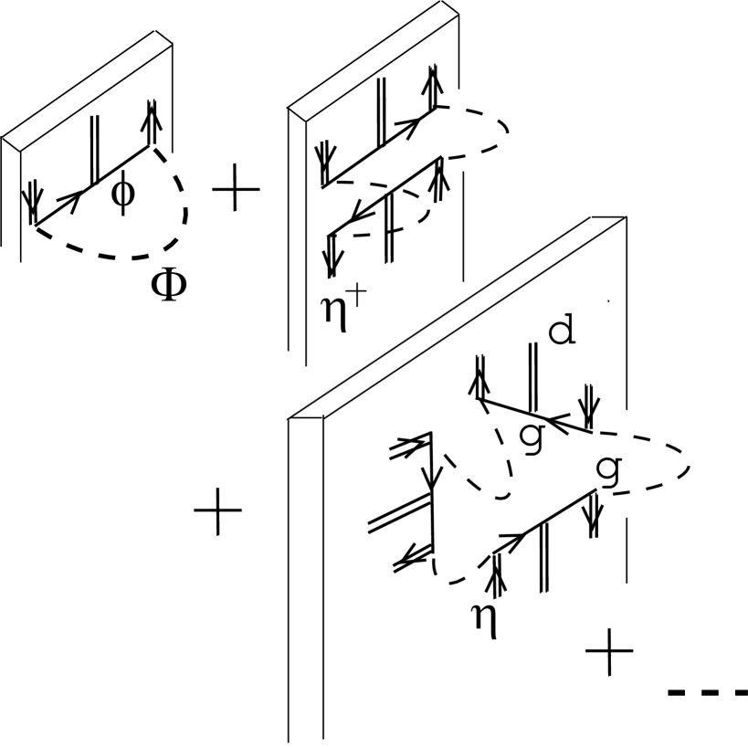
Figure 9: The diagrams contributing to the effective potential at the full (w.r.t. $g$) 1-loop level. The dotted lines represent quantum propagation of the bulk scalar $\Phi$, the directed single lines represent that of the boundary (4D) scalars $\phi,\phi^{\dagger}$. The double lines represent boundary background fields $\eta,\eta^{\dagger}$ and $d$. The ”wall” represents the ${x^{5}}=0$ brane. The corresponding eigenvalues are given by (171). This figure is the bulk-boundary generalization of FIG.2 of ref.[9].

8 Conclusion

We have analyzed the quantum structure of a bulk-boundary system by taking the example of the Mirabelli-Peskin model. The analysis is newly formulated by the background field method. Feynman rules for the perturbative calculation are presented. We focus on the (1-loop) effective potential and the vacuum energy. It is confirmed that the singular terms well behave with the Kaluza-Klein modes summation. The whole effect can be regarded as some deformation of the 4D quantization. Its 4D reduction by $l\rightarrow 0$ is confirmed in the renormalization group calculation. The characteristic relation among the 4D-momentum ${\bar{k}}$, UV-cutoff $\Lambda$, and the IR-cutoff($S^{1}$ radius) $l$ appears. It comes from the requirement to escape from the linear divergence. The relation is the same one as in the lattice domain wall fermion. In addition to the bulk scalar $\Phi$, the extra component of the bulk vector $A^{5}$ plays an important role in determining the vacuum. Especially their localized configurations are exploited. In the treatment, the vacuum is generalized in the sense that scalars may depend on the extra coordinate ${x^{5}}$. In the intermediate stage, we have obtained a new type Casimir energy in addition to the ordinary type by Appelquist and Chodos. The obtained result of the effective potential includes the bulk-boundary generalization of the Coleman-Weinberg’s case.

We hope the present analysis advances further development of the brane world physics.

Acknowledgment

The authors thank N. Sakai for valuable comments when this work, still at the primitive stage, was presented at the Chubu Summer School 2002 (Tsumagoi, Gunma, Japan, 2002.8.30-9.2). Parts of the present results were presented at the seminar of DAMTP, Univ. of Cambridge (2003.1.24). The encouraging comment by G.W. Gibbons is much appreciated. Some results were also presented at the annual meetings of the Physical Society of Japan (Rikkyo Univ.,Tokyo, Japan, 2002.9.13-16; Thohoku Gakuin Univ.,Sendai,Japan, 2003.3.28-31; Miyazaki World Convention Center Summit,Miyazaki,Japan,2003.9.9-12) and SUSY04(Jun.17-23, Tsukuba, Japan). The authors thank the audience for stimulated comments.

9 Appendix A: Effective Potential of Super QED

Now we consider the super QED. The action is most concisely described by one vector

superfield $V$ and two chiral ones $S$ (charge $g$) and $R$ (charge $-g$):

$$S=\int d^{4}xd^{2}\theta d^{2}{\bar{\theta}}({\bar{S}}{\rm e}^{gV}S+{\bar{R}}{\rm e}^{-gV}R)+\left\{\int d^{4}xd^{2}\theta(\frac{1}{4}WW+mSR)+\mbox{h.c.}\right\}{\quad,}$$

$$W^{\alpha}=-\frac{1}{4}{\bar{D}}^{2}D^{\alpha}V{\quad,}\quad V=-\theta\sigma^{m}{\bar{\theta}}~{}v_{m}+i\theta\theta{\bar{\theta}}~{}{\bar{\lambda}}-i{\bar{\theta}}{\bar{\theta}}\theta~{}\lambda+{\frac{1}{2}}\theta\theta{\bar{\theta}}{\bar{\theta}}~{}D{\quad,}$$

$$S=A_{S}(y)+\sqrt{2}\theta~{}\psi_{S}(y)+\theta\theta~{}F_{S}(y)\ ,\ R=A_{R}(y)+\sqrt{2}\theta~{}\psi_{R}(y)+\theta\theta~{}F_{R}(y)\ ,$$

$$y^{m}=x^{m}+i\theta\sigma^{m}{\bar{\theta}}{\quad.}$$ (173)

We focus on the scalar sector of the effective potential, based on the following points: 1) Lorentz invariance of the vacuum, 2) the 1-loop contribution from the non-scalar fields (spinors, vectors) can be recovered by taking ”supersymmetric boundary condition”. We put the condition.

$$v_{m}=0{\quad,}\quad\lambda={\bar{\lambda}}=0{\quad,}\quad\psi_{S}=\psi_{R}=0{\quad.}$$ (174)

Then the Lagragian of the super QED reduces to the simple form.

$${\cal L}[A_{S},F_{S};A_{R},F_{R};D:\ m,g]=$$

$$\{{\bar{A}}_{S}\partial_{m}\partial^{m}A_{S}+{\bar{F}}_{S}F_{S}+m(A_{R}F_{S}+{\bar{A}}_{R}{\bar{F}}_{S})+R\leftrightarrow S\}$$

$$+\{{\frac{1}{2}}D^{2}+{\frac{1}{2}}gD({\bar{A}}_{S}A_{S}-{\bar{A}}_{R}A_{R})\}{\quad.}$$ (175)

Now we expand all scalar fields around the background constants ($a_{S},f_{S},\cdots$).

$$A_{S}\rightarrow a_{S}+A_{S}\ ,\ F_{S}\rightarrow f_{S}+F_{S}\ ,\ D\rightarrow d+D\ ,\ {\bar{A}}_{S}\rightarrow{\bar{a}}_{S}+{\bar{A}}_{S}\ ,\ {\bar{F}}\rightarrow{\bar{f}}_{S}+{\bar{F}}_{S}{\quad,}$$ (176)

and similarly for $A_{R},{\bar{A}}_{R},F_{R},{\bar{F}}_{R}$.

The effective potential $V^{eff}[a,{\bar{a}},f,{\bar{f}},d]$ is defined as

$$\exp\{-i{\int d^{4}x}V^{eff}[a,{\bar{a}},f,{\bar{f}},d]\}=\int({\cal D}A{\cal D}F{\cal D}{\bar{A}}{\cal D}{\bar{F}})_{S,R}{\cal D}D$$

$$\times\exp i{\int d^{4}x}\left\{{\cal L}[a+A,{\bar{a}}+{\bar{A}},f+F,{\bar{f}}+{\bar{F}},d+D]-\left.\frac{\delta{\cal L}}{\delta\Phi^{I}}\right|_{b}\Phi^{I}\right\}$$

$$=\exp i\{-{\int d^{4}x}V^{eff}_{0}\}\times\int({\cal D}A{\cal D}F{\cal D}{\bar{A}}{\cal D}{\bar{F}})_{S,R}{\cal D}D$$

$$\times\exp i{\int d^{4}x}\left\{{\cal L}_{2}+(\mbox{quantum field})^{3}\ \mbox{and higher-order}\ \right\}{\quad,}$$ (177)

where $(\Phi^{I})\equiv(A_{S,R}\,,F_{S,R}\,,{\bar{A}}_{S,R}\,,{\bar{F}}_{S,R}\,,D)$ are treated as the quantum fields and $(\Phi^{I})|_{b}\equiv(a_{S,R}\,,f_{S,R}\,,{\bar{a}}_{S,R}\,,{\bar{f}}_{S,R}\,,d)$ are as the background fields. $-V^{eff}_{0}$ is the tree (zero-th order) part and is given below. ${\cal L}_{2}$ is the quadratic part and will be given in (194). The zero-th order is

$${\cal L}_{0}=-V^{eff}_{0}=\{{\bar{f}}_{S}f_{S}+m(a_{R}f_{S}+{\bar{a}}_{R}{\bar{f}}_{S})+R\leftrightarrow S\}+{\frac{1}{2}}d^{2}+\frac{g}{2}d({\bar{a}}_{S}a_{S}-{\bar{a}}_{R}a_{R}){\quad.}$$ (178)

The first order is given by

$${\cal L}_{1}=\left.\frac{\delta{\cal L}}{\delta\Phi^{I}}\right|_{b}\Phi^{I}=\{{\bar{F}}_{S}(f_{S}+m{\bar{a}}_{R})+({\bar{f}}_{S}+ma_{R})F_{S}+R\leftrightarrow S\}$$

$$+\{A_{R}(mf_{S}-\frac{g}{2}d{\bar{a}}_{R})+A_{S}(mf_{R}+\frac{g}{2}d{\bar{a}}_{S})+\mbox{h.c.}\}+D\{d+\frac{g}{2}({\bar{a}}_{S}a_{S}-{\bar{a}}_{R}a_{R})\}\ .$$ (179)

There is a special choice of the background constants, the on-shell condition:

$$f_{S}+m{\bar{a}}_{R}=0{\quad,}\quad f_{R}+m{\bar{a}}_{S}=0{\quad,}\quad mf_{S}-\frac{g}{2}d{\bar{a}}_{R}=0{\quad,}\quad mf_{R}+\frac{g}{2}d{\bar{a}}_{S}=0{\quad,}$$

$$d+\frac{g}{2}({\bar{a}}_{S}a_{S}-{\bar{a}}_{R}a_{R})=0{\quad,}$$ (180)

and their complex conjugate. This is the solution of the field equation: ${\cal L}_{1}=0$. When the background constants satisfy the above equations, the tree effective potential $V^{eff}_{0}$ takes

$$V^{eff}_{0}|_{\mbox{on-shell}}={\bar{f}}_{S}f_{S}+{\bar{f}}_{R}f_{R}+{\frac{1}{2}}d^{2}\geq 0{\quad.}$$ (181)

From the results (180) and (181), the (classical) vacuum is given by the solution: $f_{S}=f_{R}=0,\ d=0,\ a_{R}=a_{S}=0$ where $m\neq 0$ is assumed. In the following analysis, however, we consider the general case of the background constants. (We do not require the on-shell condition: ${\cal L}_{1}=0$.)

The second order part ${\cal L}_{2}$ is given by taking the quadratic terms with respect to the quantum fields ($A_{S,R}\,,F_{S,R}\,,{\bar{A}}_{S,R}\,,{\bar{F}}_{S,R}\,,D$). ${\cal L}_{2}$ can be expressed in the following form, where $F,{\bar{F}}$-involved terms are separated.

$${\cal L}_{2}={\frac{1}{2}}\left(\begin{array}[]{ccccc}{\bar{A}}_{S}&A_{S}&{\bar{A}}_{R}&A_{R}&D\end{array}\right){\bf A}\left(\begin{array}[]{c}A_{S}\\ {\bar{A}}_{S}\\ A_{R}\\ {\bar{A}}_{R}\\ D\end{array}\right)+\{{\bar{F}}_{S}F_{S}+m(A_{R}F_{S}+{\bar{A}}_{R}{\bar{F}}_{S})+R\leftrightarrow S\}\ ,$$ (188)

$${\bf A}=\left(\begin{array}[]{ccccc}\Box+dg/2&0&0&0&ga_{S}/2\\ 0&\Box+dg/2&0&0&g{\bar{a}}_{S}/2\\ 0&0&\Box-dg/2&0&-ga_{R}/2\\ 0&0&0&\Box-dg/2&-g{\bar{a}}_{R}/2\\ g{\bar{a}}_{S}/2&ga_{S}/2&-g{\bar{a}}_{R}/2&-ga_{R}/2&1\end{array}\right){\quad.}$$ (194)

The above matrix ${\bf A}$ is the same as that in Ref.[17]. Integrating out all auxiliary fields $D,F_{S},F_{R},{\bar{F}}_{S},{\bar{F}}_{R}$ using ”squaring equations”:

$$\left\{{\frac{1}{2}}g(a_{S}{\bar{A}}_{S}-a_{R}{\bar{A}}_{R})D+\mbox{c.c.}\right\}+{\frac{1}{2}}D^{2}$$

$$={\frac{1}{2}}\{D+\frac{g}{2}(a_{S}{\bar{A}}_{S}-a_{R}{\bar{A}}_{R}+\mbox{c.c.})\}^{2}-\frac{g^{2}}{8}(a_{S}{\bar{A}}_{S}-a_{R}{\bar{A}}_{R}+\mbox{c.c.})^{2}{\quad,}$$

$${\bar{F}}_{S}F_{S}+m(A_{R}F_{S}+{\bar{A}}_{R}{\bar{F}}_{S})+(S\leftrightarrow R)$$

$$=({\bar{F}}_{S}+mA_{R})(F_{S}+m{\bar{A}}_{R})-m^{2}A_{R}{\bar{A}}_{R}+(S\leftrightarrow R){\quad,}$$ (195)

${\cal L}_{2}$ reduces to

$${\cal L}_{2}^{\prime}={\bar{A}}_{S}\Box A_{S}+{\bar{A}}_{R}\Box A_{R}+{\frac{1}{2}}\left(\begin{array}[]{cccc}{\bar{A}}_{S}&A_{S}&{\bar{A}}_{R}&A_{R}\end{array}\right){\bf M}\left(\begin{array}[]{c}A_{S}\\ {\bar{A}}_{S}\\ A_{R}\\ {\bar{A}}_{R}\end{array}\right)\ ,\ \Box=\partial_{m}\partial^{m}\ ,$$ (201)

$${\bf M}=\left(\begin{array}[]{cccc}-Ga_{S}{\bar{a}}_{S}+{\tilde{d}}-m^{2}&-G{\bar{a}}_{S}{\bar{a}}_{S}&Ga_{R}{\bar{a}}_{S}&G{\bar{a}}_{R}{\bar{a}}_{S}\\ -Ga_{S}a_{S}&-G{\bar{a}}_{S}a_{S}+{\tilde{d}}-m^{2}&Ga_{R}a_{S}&G{\bar{a}}_{R}a_{S}\\ Ga_{S}{\bar{a}}_{R}&G{\bar{a}}_{S}{\bar{a}}_{R}&-Ga_{R}{\bar{a}}_{R}-{\tilde{d}}-m^{2}&-G{\bar{a}}_{R}{\bar{a}}_{R}\\ Ga_{S}a_{R}&G{\bar{a}}_{S}a_{R}&-Ga_{R}a_{R}&-G{\bar{a}}_{R}a_{R}-{\tilde{d}}-m^{2}\end{array}\right).$$ (206)

(207)

where $G\equiv g^{2}/4,\ {\tilde{d}}\equiv dg/2$. The four eigenvalues of ${\bf M}$ are obtained as

$$\lambda_{1}={\tilde{d}}-m^{2}=\frac{g}{2}d-m^{2}{\quad,}\quad\lambda_{2}={\tilde{d}}-m^{2}-2Ga_{S}{\bar{a}}_{S}=\frac{g}{2}d-m^{2}-\frac{g^{2}}{2}a_{S}{\bar{a}}_{S}{\quad,}$$

$$\lambda_{3}=-{\tilde{d}}-m^{2}=-\frac{g}{2}d-m^{2}{\quad,}\quad\lambda_{4}=-{\tilde{d}}-m^{2}-2Ga_{R}{\bar{a}}_{R}=-\frac{g}{2}d-m^{2}-\frac{g^{2}}{2}a_{R}{\bar{a}}_{R}{\quad.}$$ (208)

Then the 1-loop contribution is given as

$$\int({\cal D}A{\cal D}{\bar{A}})_{S,R}\exp i{\int d^{4}x}{\cal L}_{2}^{\prime}$$

$$=\left[\det(\Box+\lambda_{1})(\Box+\lambda_{2})(\Box+\lambda_{3})(\Box+\lambda_{4})\right]^{-{\frac{1}{2}}}=\exp-i{\int d^{4}x}V^{eff}_{1-loop}\ ,\$$

$$V^{eff}_{1-loop}={\frac{1}{2}}{\rm Tr\,}\sum_{i=1}^{4}\ln(\Box+\lambda_{i}){\quad.}$$ (209)

Normalizing $V^{eff}_{1-loop}$ at $d=0$, from the requirement of the supersymmetric boundary condition (Sect.2), we finally obtain

$$V^{eff}_{1-loop}-V^{eff}_{1-loop}|_{d=0}={\frac{1}{2}}\int\frac{d^{4}k}{(2\pi)^{4}}\left\{\ln\left(1-(\frac{g}{2})^{2}\frac{d^{2}}{(k^{2}+m^{2})^{2}}\right)\right.$$

$$+\ln\left(1-(\frac{g}{2})^{2}\frac{d^{2}}{(k^{2}+m^{2}+g^{2}a_{S}{\bar{a}}_{S}/2)(k^{2}+m^{2}+g^{2}a_{R}{\bar{a}}_{R}/2)}\right.$$

$$\left.\left.+\frac{g}{2}\frac{g^{2}}{2}\frac{d(a_{S}{\bar{a}}_{S}-a_{R}{\bar{a}}_{R})}{(k^{2}+m^{2}+g^{2}a_{S}{\bar{a}}_{S}/2)(k^{2}+m^{2}+g^{2}a_{R}{\bar{a}}_{R}/2)}\right)\right\}$$

$$\approx\left(-\frac{g^{4}}{4}d^{2}+\frac{g^{3}}{8}d(a_{S}{\bar{a}}_{S}-a_{R}{\bar{a}}_{R})\right)\int\frac{d^{4}k}{(2\pi)^{4}}\frac{1}{(k^{2}+m^{2})^{2}}+O(g^{4}){\quad.}$$ (210)

The last approximate form is logarithmically divergent. We introduce a counterterm $\Delta{\cal L}$ as in the following form.

$$V_{R}=V^{eff}_{0}+V^{eff}_{1-loop}-V^{eff}_{1-loop}|_{d=0}-\Delta{\cal L}{\quad,}$$

$$V^{eff}_{0}=-{\frac{1}{2}}d^{2}-{\frac{1}{2}}gd({\bar{a}}_{S}a_{S}-{\bar{a}}_{R}a_{R})+\cdots{\quad,}$$

$$\Delta{\cal L}={\frac{1}{2}}\Delta Z\,d^{2}+{\frac{1}{2}}\Delta g\,d({\bar{a}}_{S}a_{S}-{\bar{a}}_{R}a_{R}){\quad,}$$ (211)

where $V^{eff}_{0}$ is the tree part of the potential (178). $Z=1+\Delta Z$ and $g_{b}=g+\Delta g$ are the wave-function renormalization constant of $D$ and the bare coupling constant, respectively. We fix $\Delta Z$ and $\Delta g$ by imposing the following renormalization condition.

$$\left.\frac{dV_{R}}{d(d^{2})}\right|_{d=0,a={\bar{a}}=0}=-{\frac{1}{2}}{\quad,}$$

$$\left.\frac{dV_{R}}{d[d({\bar{a}}_{S}a_{S}-{\bar{a}}_{R}a_{R})]}\right|_{d=0,a={\bar{a}}=0}=-{\frac{1}{2}}g{\quad.}$$ (212)

Hence $\Delta Z$ and $\Delta g$ are fixed as

$$\Delta Z=-\frac{g^{2}}{2}\int_{|k|\leq\Lambda}\frac{d^{4}k}{(2\pi)^{4}}\frac{1}{(k^{2}+m^{2})^{2}}=(-\frac{g^{2}}{2})\frac{-1}{16\pi^{2}}\ln\frac{\Lambda^{2}}{m^{2}}{\quad,}$$

$$\Delta g=\frac{g^{3}}{4}\int_{|k|\leq\Lambda}\frac{d^{4}k}{(2\pi)^{4}}\frac{1}{(k^{2}+m^{2})^{2}}=(\frac{g^{3}}{4})\frac{-1}{16\pi^{2}}\ln\frac{\Lambda^{2}}{m^{2}}{\quad,}$$ (213)

where $\Lambda$ is the momentum cutoff, $|k^{2}|\leq\Lambda^{2}$. Then the $\beta$-function of the coupling and the anomalous dimension $\gamma$ of the $D$ field are given as

$$g_{b}=g+\Delta g=g(1-\frac{g^{2}}{4}\frac{1}{16\pi^{2}}\ln\frac{\Lambda^{2}}{m^{2}}){\quad,}$$

$$0\equiv\frac{d}{d(\ln\Lambda)}\ln g_{b}=\frac{d\ln g}{d(\ln\Lambda)}(1+O(g^{2}))-\frac{g^{2}}{2}\frac{1}{16\pi^{2}}+O(g^{2}){\quad,}$$

$$\beta(g)\equiv\frac{1}{g}\frac{dg}{d\ln\Lambda}=\frac{g^{2}}{2}\frac{1}{16\pi^{2}}{\quad,}$$

$$Z=1+\Delta Z{\quad,}\quad\gamma=\frac{\partial}{\partial\ln\Lambda}\ln Z=\frac{g^{2}}{16\pi^{2}}+O(g^{4}){\quad.}$$ (214)

Finally the on-shell potential is obtained as

$$V^{1-loop}_{R}\equiv V^{eff}_{1-loop}-V^{eff}_{1-loop}|_{d=0}-\Delta{\cal L}{\quad,}$$

$$V_{R}|_{on-shell}=(V^{eff}_{0}+V^{1-loop}_{R})|_{on-shell}{\quad,}$$

$$V^{eff}_{0}|_{\mbox{on-shell}}={\bar{f}}_{S}f_{S}+{\bar{f}}_{R}f_{R}+{\frac{1}{2}}d^{2}\quad(\mbox{eq.(\ref{qed8})}){\quad,}$$

$$V^{1-loop}_{R}|_{on-shell}=\frac{1}{64\pi^{2}}\left[-g^{2}d^{2}+(m^{4}+\frac{g^{2}}{4}d^{2})\ln(1+\frac{g}{2m^{2}}d)(1-\frac{g}{2m^{2}}d)\right.$$

$$-gm^{2}d\,\ln\frac{1-\frac{g}{2m^{2}}d}{1+\frac{g}{2m^{2}}d}-m^{4}(1+\frac{g^{2}}{2m^{4}}{\bar{f}}_{S}f_{S})^{2}\ln\frac{1+\frac{g^{2}}{2m^{4}}{\bar{f}}_{S}f_{S}}{1+\frac{g^{2}}{2m^{4}}{\bar{f}}_{S}f_{S}+\frac{g}{2m^{2}}d}$$

$$-m^{4}(1+\frac{g^{2}}{2m^{4}}{\bar{f}}_{R}f_{R})^{2}\ln\frac{1+\frac{g^{2}}{2m^{4}}{\bar{f}}_{R}f_{R}}{1+\frac{g^{2}}{2m^{4}}{\bar{f}}_{R}f_{R}-\frac{g}{2m^{2}}d}$$

$$+\frac{g^{2}}{4}d^{2}\,\ln\left\{(1+\frac{g^{2}}{2m^{4}}{\bar{f}}_{S}f_{S}+\frac{g}{2m^{2}}d)(1+\frac{g^{2}}{2m^{4}}{\bar{f}}_{R}f_{R}-\frac{g}{2m^{2}}d)\right\}$$

$$+gm^{2}d\,(1+\frac{g^{2}}{2m^{4}}{\bar{f}}_{S}f_{S})\ln(1+\frac{g^{2}}{2m^{4}}{\bar{f}}_{S}f_{S}+\frac{g}{2m^{2}}d)$$

$$\left.-gm^{2}d\,(1+\frac{g^{2}}{2m^{4}}{\bar{f}}_{R}f_{R})\ln(1+\frac{g^{2}}{2m^{4}}{\bar{f}}_{R}f_{R}-\frac{g}{2m^{2}}d)\right]{\quad.}$$ (215)

For the case: $m=1,{\bar{f}}_{S}f_{S}={\bar{f}}_{R}f_{R}\equiv{\bar{f}}f$; the above potentials, $V^{eff}_{0}|_{\mbox{on-shell}}$ and $V^{1-loop}_{R}|_{\mbox{on-shell}}$, are depicted in Fig.10. The shape of the 1-loop correction is not the Coleman-Weinberg type. Positive definiteness is preserved after the renormalization. The potential minimum does not change. The minimum ($f_{S}=f_{R}=0,d=0,a_{S}=a_{R}=0$) corresponds to the SUSY invariant vacuum. This shows a characteristic feature of the SUSY theory, that is, it is stable against the quantum effect.

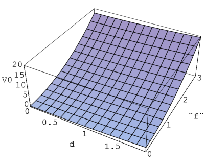
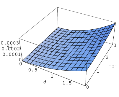
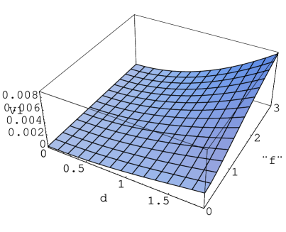
Figure 10: The effective potential of SQED(215) for the case: $m=1,{\bar{f}}_{S}f_{S}={\bar{f}}_{R}f_{R}\equiv{\bar{f}}f$. The tree part ($V^{eff}_{0}|_{\mbox{on-shell}}\equiv V_{0}$, above) and the 1-loop correction part ($V^{1-loop}_{R}|_{\mbox{on-shell}}\equiv V_{1}$, below) are depicted for $g=0.3$(left), $g=1$(right). The axis-ranges are $0\leq d\leq 1.9,0\leq|f|\equiv\sqrt{{\bar{f}}f}\leq 3$.

The form of the potential $V_{R}$ does not essentially change from the tree one (181). The stableness of the vacuum was already pointed out, in the counter-term calculation, by Barbieri et al[21]. We confirm it by the explicit form of the renormalized potential.

10 Appendix B: Eigenvalues of Mass Matrix ${\cal M}$ and Effective Potential of the Mirabelli-Peskin Model

The effective potential of the present bulk-boundary model can be obtained from the eigenvalues of the mass matrix ${\cal M}$ of (159) and (160). It is made of three field values $\eta,\eta^{\dagger},d_{\alpha}$, two wall ”heights”, ${\bar{a}}_{\alpha},{\bar{\varphi}}_{\alpha}$, the gauge coupling, $g$ and the boundary parameter $l$. The general case is hard to analyze explicitly. Here we consider two interesting ”sections”: A) $\eta=0,\eta^{\dagger}=0$ (bulk-boundary decoupled case); B) ${\bar{\varphi}}=0,{\bar{a}}=0$ (bulk-boundary coupled case).

10.1 Effective Potential From Matter Field Vanishing Point  — Case A) $\eta=0,\eta^{\dagger}=0$ —

In this configuration, the interaction term $g{\cal D}_{\alpha}\phi^{\dagger}T^{\alpha}\phi$ of (65) does not contribute to the bulk-boundary loop. The bulk and boundary are decoupled in the quantum fluctuation. It turns out, however, that the renormalization procedure to deal with the divergences due to the boundary-loop makes connection between the bulk and boundary. (See the explanation below (234).) ${\cal M}$ has the following form:

$${\left(\begin{array}[]{cc}\left(\begin{array}[]{cc}{\cal M}_{\phi^{\dagger}\phi}&0\\ 0&{\cal M}_{\phi\phi^{\dagger}}\\ \end{array}\right)_{{\alpha^{\prime}}\,{\beta^{\prime}}}&\left(\begin{array}[]{cc}0&0\\ 0&0\end{array}\right)_{{\alpha^{\prime}}\,n\beta}\\ \left(\begin{array}[]{cc}0&0\\ 0&0\end{array}\right)_{m\alpha\,{\beta^{\prime}}}&\left(\begin{array}[]{cc}{\cal M}_{\Phi\Phi}&{\cal M}_{\Phi A}\\ {\cal M}_{A\Phi}&{\cal M}_{AA}\end{array}\right)_{m\alpha\,n\beta}\end{array}\right)}{\quad.}$$ (226)

The components are given, from (160), as

$${\cal M}_{\phi^{\dagger}_{\alpha^{\prime}}\phi_{\beta^{\prime}}}=\partial^{2}\delta_{{\alpha^{\prime}}{\beta^{\prime}}}+gd_{\gamma}(T^{\gamma})_{{\alpha^{\prime}}{\beta^{\prime}}}{\quad,}\$$

$${\cal M}_{\phi_{\alpha^{\prime}}\phi^{\dagger}_{\beta^{\prime}}}=\partial^{2}\delta_{{\alpha^{\prime}}{\beta^{\prime}}}+gd_{\gamma}(T^{\gamma})_{{\beta^{\prime}}{\alpha^{\prime}}}{\quad,}\$$

$${\cal M}_{\Phi_{m\alpha}\Phi_{n\beta}}=-\{-\partial^{2}+({\frac{n\pi}{l}})^{2}\}\delta_{mn}\delta_{\alpha\beta}-g^{2}f_{\alpha\delta\tau}f_{\beta\gamma\tau}{\bar{a}}_{\delta}{\bar{a}}_{\gamma}\delta_{mn}+\frac{4g}{l}f_{{\alpha\beta}\gamma}{\bar{a}}_{\gamma}mQ_{mn}{\quad,}$$

$${\cal M}_{\Phi_{m\alpha}A_{n\beta}}=g^{2}f_{{\alpha\beta}\tau}f_{\gamma\delta\tau}{\bar{a}}_{\gamma}{\bar{\varphi}}_{\delta}\delta_{mn}-g^{2}f_{\gamma\alpha\tau}f_{\beta\delta\tau}{\bar{a}}_{\gamma}{\bar{\varphi}}_{\delta}\delta_{mn}-\frac{2g}{l}f_{{\alpha\beta}\gamma}{\bar{\varphi}}_{\gamma}mQ_{mn}=M_{A_{n\beta}\Phi_{m\alpha}},$$

$${\cal M}_{A_{m\alpha}A_{n\beta}}=-\{-\partial^{2}+({\frac{n\pi}{l}})^{2}\}\delta_{mn}\delta_{\alpha\beta}-g^{2}f_{\alpha\gamma\tau}f_{\beta\delta\tau}{\bar{\varphi}}_{\gamma}{\bar{\varphi}}_{\delta}\delta_{mn}{\quad,}$$ (227)

where the integer indices $m,n$ run from 1 to $\infty$. $Q_{mn}$ is defined in (135). The singular terms, $\delta(0)$-terms, disappear. The bulk and the boundary are decoupled, hence the eigen values can be obtained separately.

For simplicity we take $SU(2)$ as the gauge group G ($f_{{\alpha\beta}\gamma}=\epsilon^{{\alpha\beta}\gamma}$) and the doublet representation for the matter fields $\phi_{\alpha^{\prime}}\ ({\alpha^{\prime}}=1,2)$.

$$T^{\alpha}={\frac{1}{2}}\sigma^{\alpha}{\quad,}\quad[T^{\alpha},T^{\beta}]=i\epsilon^{{\alpha\beta}\gamma}T^{\gamma}{\quad,}\quad{\rm Tr\,}(T^{\alpha}T^{\beta})={\frac{1}{2}}\delta^{\alpha\beta}{\quad,}$$ (228)

where $\sigma^{\alpha}(\alpha=1,2,3)$ is the Pauli sigma matrices, and $\epsilon^{123}=1$.

(Ai) boundary part
The eigenvalues of

$$\left({\cal M}_{\phi^{\dagger}_{\alpha^{\prime}}\phi_{\beta^{\prime}}}\right)=\left(\begin{array}[]{cc}-k^{2}+\frac{g}{2}d_{3}&\frac{g}{2}(d_{1}-id_{2})\\ \frac{g}{2}(d_{1}+id_{2})&-k^{2}-\frac{g}{2}d_{3}\end{array}\right){\quad,}$$ (231)

are

$$\lambda_{\pm}=-k^{2}\pm\frac{g}{2}\sqrt{d^{2}}{\quad,}\quad d^{2}\equiv{d_{1}}^{2}+{d_{2}}^{2}+{d_{3}}^{2}{\quad,}$$ (232)

The same ones are obtained for $({\cal M}_{\phi_{\alpha^{\prime}}\phi^{\dagger}_{\beta^{\prime}}})$. The effective potential can be obtained as

$${V^{eff}_{1-loop}}^{\prime}={\frac{1}{2}}{\rm Tr\,}\ln(\lambda_{+})^{2}(\lambda_{-})^{2}={\rm Tr\,}\ln\{(k^{2})^{2}-\frac{g^{2}}{4}d^{2}\}$$

$$=\int\frac{d^{4}k}{(2\pi)^{4}}[\ln(k^{2})^{2}+\ln\{1-\frac{g^{2}}{4}\frac{d^{2}}{(k^{2})^{2}}\}]{\quad.}$$ (233)

Compare this result with the super QED case (the first line of (210)). Taking the SUSY condition (see the explanation given above (37)), we reach the final answer.

$$V^{eff}_{1-loop}=\int\frac{d^{4}k}{(2\pi)^{4}}\ln\{1-\frac{g^{2}}{4}\frac{d^{2}}{(k^{2})^{2}}\}$$

$$=-\frac{g^{2}}{4}\int\frac{d^{4}k}{(2\pi)^{4}}\frac{d^{2}}{(k^{2})^{2}}+O(g^{4}){\quad.}$$ (234)

The last approximated form corresponds to (c) of (84), and is logarithmically divergent. Because $d_{\alpha}$ is given by $d_{\alpha}=(\chi^{3}-\partial_{5}\varphi+ga_{5}\times\varphi)_{\alpha}$, the UV divergence of (234) is renormalized by the bulk wave function of $X^{3}$ and $\Phi$. Here the 4D world’s connection to the bulk world appears. The quantum fluctuation within the boundary influence the bulk world through the renormalization. The boundary dynamics does not close within the brane. We do not touch on the renormalization of the bulk fields. After an appropriate renormalization, we expect the effective potential (234) leads to a similar potential to that given in App.A for the case $m=0,{\bar{f}}f=0$. (Note that the boundary theory treated in this section is chiral, whereas the Super QED treated in App.A is vector-like. ) We may conclude that, in the vacuum specified by $\eta=0,\eta^{\dagger}=0$, the renormalization works well as far as the boundary world is concerned. The 4D theory is well-defined.

(Aii) Bulk Part
Let us evaluate the eigenvalues from the bulk part. Because it does not depend on $d_{\alpha}$, this part does not contribute to the effective potential in the SUSY boundary condition. However it is important to see what terms are quantumly induced by the scalar fields. (Those terms are expected to be cancelled by the fermion and vector fields contribution.) The result depends on the ”heights” of the 4D scalars, ${\bar{a}}$ and ${\bar{\varphi}}$, in addition to the periodicity $2l$. Generally that part of the vacuum energy which depends on the boundary parameters is called ”Casimir energy”. We regard ${\bar{a}}$ and ${\bar{\varphi}}$, besides $l$, as those parameters. They correspond to the brane tension and the brane thickness in the brane world. One of most important points of the brane model is how to treat the KK-modes. We can see such a point in this calculation.

The eigenvalue equation can be written as

$$\left(\begin{array}[]{cc}{\cal M}_{\Phi_{m\alpha}\Phi_{n\beta}}&{\cal M}_{\Phi_{m\alpha}A_{n\beta}}\\ {\cal M}_{A_{m\alpha}\Phi_{n\beta}}&{\cal M}_{A_{m\alpha}A_{n\beta}}\end{array}\right)\left(\begin{array}[]{c}{\hat{\Phi}}_{n\beta}\\ {\hat{A}}_{n\beta}\end{array}\right)=\lambda\left(\begin{array}[]{c}{\hat{\Phi}}_{m\alpha}\\ {\hat{A}}_{m\alpha}\end{array}\right){\quad.}$$ (241)

From the symmetry, we can take the following general form as an eigen vector.

$${\hat{\Phi}}_{n\beta}=f_{1}(n){\bar{a}}_{\beta}+f_{2}(n){\bar{\varphi}}_{\beta}+f_{3}(n)f_{\beta\gamma\delta}{\bar{a}}_{\gamma}{\bar{\varphi}}_{\delta}{\quad,}$$

$${\hat{A}}_{n\beta}=g_{1}(n){\bar{a}}_{\beta}+g_{2}(n){\bar{\varphi}}_{\beta}+g_{3}(n)f_{\beta\gamma\delta}{\bar{a}}_{\gamma}{\bar{\varphi}}_{\delta}{\quad,}$$ (242)

where $f_{i}(n)$ and $g_{i}(n)$ are scalar quantities (with respect to the internal group transformation) which may depend on ${\bar{a}}$ and ${\bar{\varphi}}$. Through the above relation, the eigenvalue equation for ${\hat{\Phi}}$ and ${\hat{A}}$ is replaced by that for $f_{i}(n)$ and $g_{i}(n)$. The eigenvalues are obtained from the zeros of the determinant of the following matrix.

$$\begin{array}[]{c|c|c}&\begin{array}[]{ccc}f_{1}(n)&f_{2}(n)&f_{3}(n)\end{array}&\begin{array}[]{ccc}g_{1}(n)&g_{2}(n)&g_{3}(n)\end{array}\\ \hline\cr\begin{array}[]{c}{\bar{a}},m\\ {\bar{\varphi}},m\\ {\bar{a}}\times{\bar{\varphi}},m\end{array}&\mbox{{\Huge a}}&\mbox{{\Huge c}}\\ \hline\cr\begin{array}[]{c}{\bar{a}},m\\ {\bar{\varphi}},m\\ {\bar{a}}\times{\bar{\varphi}},m\end{array}&\mbox{{\Huge d}}&\mbox{{\Huge b}}\end{array}{\quad.}$$ (254)

The above 4 matrices are given as follows.

The first row equation of (241), ${\cal M}_{\Phi_{m\alpha}\Phi_{n\beta}}{\hat{\Phi}}_{n\beta}+{\cal M}_{\Phi_{m\alpha}A_{n\beta}}{\hat{A}}_{n\beta}=\lambda{\hat{\Phi}}_{m\alpha}$, gives two matrices $a$ and $c$ as

$$\mbox{{\Huge a}}={\left(\begin{array}[]{ccc}(-\lambda-k^{2}-(m\pi/l)^{2})\delta_{mn}&g^{2}{\bar{a}}\cdot{\bar{\varphi}}\delta_{mn}&-4gmQ_{mn}{\bar{a}}\cdot{\bar{\varphi}}/l\\ 0&(-\lambda-k^{2}-(m\pi/l)^{2}-g^{2}{\bar{a}}^{2})\delta_{mn}&4gmQ_{mn}{\bar{a}}^{2}/l\\ 0&-4gmQ_{mn}/l^{2}&(-\lambda-k^{2}-(m\pi/l)^{2}-g^{2}{\bar{a}}^{2})\delta_{mn}\end{array}\right)}{\quad,}$$ (258)

$$\mbox{{\Huge c}}={\left(\begin{array}[]{ccc}2g^{2}{\bar{a}}\cdot{\bar{\varphi}}\delta_{mn}&g^{2}{\bar{\varphi}}^{2}\delta_{mn}&2gmQ_{mn}{\bar{\varphi}}^{2}/l\\ -2g^{2}{\bar{a}}^{2}\delta_{mn}&-g^{2}{\bar{a}}\cdot{\bar{\varphi}}\delta_{mn}&-2gmQ_{mn}{\bar{a}}\cdot{\bar{\varphi}}/l\\ -2gmQ_{mn}/l^{4}&0&g^{2}{\bar{a}}\cdot{\bar{\varphi}}\delta_{mn}\end{array}\right)}{\quad.}$$ (262)

The second row equation of (241), ${\cal M}_{A_{m\alpha}\Phi_{n\beta}}{\hat{\Phi}}_{n\beta}+{\cal M}_{A_{m\alpha}A_{n\beta}}{\hat{A}}_{n\beta}=\lambda{\hat{A}}_{m\alpha}$, gives two matrices $d$ and $b$ as

$$\mbox{{\Huge d}}={\left(\begin{array}[]{ccc}-g^{2}{\bar{a}}\cdot{\bar{\varphi}}\delta_{mn}&-2g^{2}{\bar{\varphi}}^{2}\delta_{mn}&-2gnQ_{nm}{\bar{\varphi}}^{2}/l\\ g^{2}{\bar{a}}^{2}\delta_{mn}&2g^{2}{\bar{a}}\cdot{\bar{\varphi}}\delta_{mn}&2gnQ_{nm}{\bar{a}}\cdot{\bar{\varphi}}/l\\ 2gnQ_{nm}/l^{4}&0&g^{2}{\bar{a}}\cdot{\bar{\varphi}}\delta_{mn}\end{array}\right)}{\quad,}$$ (266)

$$\mbox{{\Huge b}}={\left(\begin{array}[]{ccc}(-\lambda-k^{2}-(m\pi/l)^{2}-g^{2}{\bar{\varphi}}^{2})\delta_{mn}&0&0\\ g^{2}{\bar{a}}\cdot{\bar{\varphi}}\delta_{mn}&(-\lambda-k^{2}-(m\pi/l)^{2})\delta_{mn}&0\\ 0&0&(-\lambda-k^{2}-(m\pi/l)^{2}-g^{2}{\bar{\varphi}}^{2})\delta_{mn}\end{array}\right)}{\quad.}$$ (270)

For convenience, let us introduce two quantities $x_{m},y_{m}$;

$$x_{m}\equiv-\lambda-k^{2}-(m\pi/l)^{2}-g^{2}{\bar{\varphi}}^{2}{\quad,}\quad y_{m}\equiv-\lambda-k^{2}-(m\pi/l)^{2}{\quad,}$$

$$x_{m}-y_{m}=-g^{2}{\bar{\varphi}}^{2}{\quad.}$$ (271)

Then the following relations are obtained.

$$\mbox{{\Huge b}}=\left(\begin{array}[]{ccc}x_{m}\delta_{mn}&0&0\\ g^{2}{\bar{a}}\cdot{\bar{\varphi}}\delta_{mn}&y_{m}\delta_{mn}&0\\ 0&0&x_{m}\delta_{mn}\end{array}\right){\quad,}$$ (275)

$$\mbox{{\Huge b}}^{-1}={\left(\begin{array}[]{ccc}\frac{1}{x_{m}}\delta_{mn}&0&0\\ -\frac{g^{2}{\bar{a}}\cdot{\bar{\varphi}}}{x_{m}y_{m}}\delta_{mn}&\frac{1}{y_{m}}\delta_{mn}&0\\ 0&0&\frac{1}{x_{m}}\delta_{mn}\end{array}\right)}{\quad,}$$ (279)

$$\mbox{{\Huge det\, b}}=\prod_{m=1}^{\infty}({x_{m}}^{2}y_{m}){\quad.}$$ (280)

Using a useful formula about general matrices ${\tilde{a}},{\tilde{b}},{\tilde{c}}$, and ${\tilde{d}}$ ($\det{\tilde{b}}\neq 0,\det{\tilde{a}}\neq 0$);

$$\det\,\left(\begin{array}[]{cc}{\tilde{a}}&{\tilde{c}}\\ {\tilde{d}}&{\tilde{b}}\end{array}\right)=\det({\tilde{a}}-{\tilde{c}}{{\tilde{b}}}^{-1}{\tilde{d}})\det{\tilde{b}}=\det{\tilde{a}}\det({\tilde{b}}-{\tilde{d}}{{\tilde{a}}}^{-1}{\tilde{c}}){\quad,}$$ (283)

we can decompose the determinant of the matrix (254). The components of the matrix ${\cal A}\equiv a-c{b}^{-1}d$ are explicitly written as

$${\cal A}\quad=\quad\begin{array}[]{c|ccc}&f_{1}(n)&f_{2}(n)&f_{3}(n)\\ \hline\cr{\bar{a}},m&{\cal A}_{11}&{\cal A}_{12}&{\cal A}_{13}\\ {\bar{\varphi}},m&{\cal A}_{21}&{\cal A}_{22}&{\cal A}_{23}\\ {\bar{a}}\times{\bar{\varphi}},m&{\cal A}_{31}&{\cal A}_{32}&{\cal A}_{33}\end{array}{\quad,}$$ (288)

$$({\cal A}_{11})_{mn}=y_{m}\delta_{mn}-g^{4}\left\{({\bar{a}}\cdot{\bar{\varphi}})^{2}\frac{1}{x_{m}}(-2+\frac{g^{2}{\bar{\varphi}}^{2}}{y_{m}})+\frac{{\bar{\varphi}}^{2}{\bar{a}}^{2}}{y_{m}}\right\}\delta_{mn}-4\frac{g^{2}{\bar{\varphi}}^{2}}{l^{2}}mn\sum_{j}\frac{Q_{mj}Q_{nj}}{x_{j}}{\quad,}$$

$$({\cal A}_{12})_{mn}=g^{2}{\bar{a}}\cdot{\bar{\varphi}}\left\{1+2g^{2}\frac{{\bar{\varphi}}^{2}}{x_{m}}\right\}\delta_{mn}{\quad,}\quad({\cal A}_{13})_{mn}=-\frac{{\bar{a}}\cdot{\bar{\varphi}}}{l}Q_{mn}\left\{4gm+2g^{3}{\bar{\varphi}}^{2}(\frac{n}{x_{m}}+\frac{m}{x_{n}})\ \right\}{\quad,}$$

$$({\cal A}_{21})_{mn}=-g^{4}\frac{{\bar{a}}\cdot{\bar{\varphi}}}{x_{m}}\left\{{\bar{a}}^{2}+\frac{g^{2}}{y_{m}}({\bar{a}}^{2}{\bar{\varphi}}^{2}-({\bar{a}}\cdot{\bar{\varphi}})^{2})\right\}\delta_{mn}+4\frac{g^{2}{\bar{a}}\cdot{\bar{\varphi}}}{l^{2}}mn\sum_{j}\frac{Q_{mj}Q_{nj}}{x_{j}}\ ,$$

$$({\cal A}_{22})_{mn}=\left\{y_{m}-g^{2}{\bar{a}}^{2}-\frac{2g^{4}}{x_{m}}(2{\bar{a}}^{2}{\bar{\varphi}}^{2}-({\bar{a}}\cdot{\bar{\varphi}})^{2})\right\}\delta_{mn}{\quad,}$$

$$({\cal A}_{23})_{mn}=\frac{Q_{mn}}{l}\left\{4g{\bar{a}}^{2}m+2g^{3}(\frac{n}{x_{m}}-\frac{m}{x_{n}})({\bar{a}}^{2}{\bar{\varphi}}^{2}-({\bar{a}}\cdot{\bar{\varphi}})^{2})\right\}{\quad,}$$

$$({\cal A}_{31})_{mn}=2\frac{g^{3}{\bar{a}}\cdot{\bar{\varphi}}}{l^{4}}Q_{mn}(\frac{n}{x_{m}}-\frac{m}{x_{n}}){\quad,}\quad({\cal A}_{32})_{mn}=-\frac{Q_{mn}}{l^{4}}\left(4gm+4g^{3}{\bar{\varphi}}^{2}\frac{m}{x_{n}}\right){\quad,}$$

$$({\cal A}_{33})_{mn}=\left\{y_{m}-g^{2}{\bar{a}}^{2}-g^{4}\frac{({\bar{a}}\cdot{\bar{\varphi}})^{2}}{x_{m}}\right\}\delta_{mn}-4\frac{g^{2}{\bar{\varphi}}^{2}}{l^{2}}mn\sum_{j}\frac{Q_{mj}Q_{nj}}{x_{j}}{\quad,}$$ (289)

where the repeated integer suffixes do not mean the summation. The summation should be taken only where the symbol $\sum_{j}$ appears.

Let us evaluate the eigenvalues $\lambda$ from the zeros of $\det{\cal A}$. General case is technically difficult. We consider the following special cases.

We consider the following limit:

$${\hat{g}}^{2}\equiv\frac{g^{2}}{l}=\mbox{fixed}\ll 1{\quad,}\quad{\hat{a}}=\sqrt{l}{\bar{a}}=\mbox{fixed}{\quad,}\quad{\hat{\varphi}}=\sqrt{l}{\bar{\varphi}}=\mbox{fixed}{\quad,}$$

$$l\rightarrow\infty{\quad.}\quad\quad\quad\quad\quad\quad\quad\quad\quad$$ (290)

This is the situation where the circle is large compared with the inverse of the domain wall height. (${\hat{a}}$ and ${\hat{\varphi}}$ have the dimension of $M$. ) Then the elements of ${\cal A}$ reduce to

$$({\cal A}_{11})_{mn}=y\delta_{mn}-{\hat{g}}^{4}\left\{({\hat{a}}\cdot{\hat{\varphi}})^{2}\frac{1}{x}(-2+\frac{{\hat{g}}^{2}{\hat{\varphi}}^{2}}{y})+\frac{{\hat{\varphi}}^{2}{\hat{a}}^{2}}{y}\right\}\delta_{mn}{\quad,}$$

$$({\cal A}_{12})_{mn}={\hat{g}}^{2}{\hat{a}}\cdot{\hat{\varphi}}\left\{1+2{\hat{g}}^{2}\frac{{\hat{\varphi}}^{2}}{x}\right\}\delta_{mn}{\quad,}\quad({\cal A}_{13})_{mn}=0{\quad,}$$

$$({\cal A}_{21})_{mn}=-{\hat{g}}^{4}\frac{{\hat{a}}\cdot{\hat{\varphi}}}{x}\left\{{\hat{a}}^{2}+\frac{{\hat{g}}^{2}}{y}({\hat{a}}^{2}{\hat{\varphi}}^{2}-({\hat{a}}\cdot{\hat{\varphi}})^{2})\right\}\delta_{mn}\ ,$$

$$({\cal A}_{22})_{mn}=\left\{y-{\hat{g}}^{2}{\hat{a}}^{2}-\frac{2{\hat{g}}^{4}}{x}(2{\hat{a}}^{2}{\hat{\varphi}}^{2}-({\hat{a}}\cdot{\hat{\varphi}})^{2})\right\}\delta_{mn}{\quad,}$$

$$({\cal A}_{23})_{mn}=0{\quad,}$$

$$({\cal A}_{31})_{mn}=0{\quad,}\quad({\cal A}_{32})_{mn}=0{\quad,}$$

$$({\cal A}_{33})_{mn}=\left\{y-{\hat{g}}^{2}{\hat{a}}^{2}-{\hat{g}}^{4}\frac{({\hat{a}}\cdot{\hat{\varphi}})^{2}}{x}\right\}\delta_{mn}{\quad,}$$ (291)

where $x\equiv-\lambda-k^{2}-{\hat{g}}^{2}{\hat{\varphi}}^{2},\ y\equiv-\lambda-k^{2}$. We notice, in this limit, $Q_{mn}$-terms disappear. In the ”propagator” terms $x_{m},y_{m}$, KK-mass terms $m^{2}\pi^{2}/l^{2}$ disappear. All KK-modes equally contribute to the vacuum energy. The condition $0=\det{\cal A}=\det{\cal A}_{33}\det{\cal A}_{22}\det({\cal A}_{11}-{\cal A}_{12}{{\cal A}_{22}}^{-1}{\cal A}_{21})$ gives us the following eigenvalues.
(i) $\det{\cal A}_{33}=0$ gives two eigenvalues $\lambda_{1},\lambda_{2}$ whose product is given by

$$\lambda_{1}\lambda_{2}=(k^{2}+{\hat{g}}^{2}{\hat{\varphi}}^{2})(k^{2}+{\hat{g}}^{2}{\hat{a}}^{2})-{\hat{g}}^{4}({\hat{a}}\cdot{\hat{\varphi}})^{2}{\quad.}$$ (292)

(ii) $\det{\cal A}_{22}=0$ gives $\lambda_{3},\lambda_{4}$ whose product is

$$\lambda_{3}\lambda_{4}=(k^{2})^{2}+k^{2}{\hat{g}}^{2}({\hat{\varphi}}^{2}+{\hat{a}}^{2})+{\hat{g}}^{4}(-3{\hat{\varphi}}^{2}{\hat{a}}^{2}+({\hat{a}}\cdot{\hat{\varphi}})^{2}){\quad.}$$ (293)

(iii) $\det({\cal A}_{11}-{\cal A}_{12}{{\cal A}_{22}}^{-1}{\cal A}_{21})=0$ gives $\lambda_{5},\lambda_{6},\lambda_{7},\lambda_{8},\lambda_{9}$ whose product is given by

$$\lambda_{5}\lambda_{6}\lambda_{7}\lambda_{8}\lambda_{9}=-(k^{2}+{\hat{g}}^{2}{\hat{\varphi}}^{2})\{(k^{2})^{2}+{\hat{g}}^{4}(({\hat{a}}\cdot{\hat{\varphi}})^{2}-{\hat{a}}^{2}{\hat{\varphi}}^{2})\}$$

$$\{(k^{2})^{2}+{\hat{g}}^{2}k^{2}({\hat{a}}^{2}+{\hat{\varphi}}^{2})+3{\hat{g}}^{4}(({\hat{a}}\cdot{\hat{\varphi}})^{2}-{\hat{a}}^{2}{\hat{\varphi}}^{2})\}{\quad.}$$ (294)

In particular, for the special case ${\hat{a}}=0$, the nontrivial factor is only $k^{2}+{\hat{g}}^{2}{\hat{\varphi}}^{2}$. Hence each KK-mode equally contribute to the vacuum energy as

$$V^{eff}_{1KK-mode}\propto\int\frac{d^{4}k}{(2\pi)^{4}}\ln\{1+{\hat{g}}^{2}\frac{{\hat{\varphi}}^{2}}{k^{2}}\}{\quad.}$$ (295)

This quantity is quadratically divergent. After an appropriate normalization, which we do not know precisely, the final form should become, based on the dimensional analysis, the following.

$$\frac{1}{l}\,V^{eff}_{1-loop}={\hat{g}}^{2}(c_{1}\frac{{\hat{\varphi}}^{2}}{l^{3}}+c_{2}\frac{{\hat{a}}^{2}}{l^{3}}+c_{3}\frac{{\hat{a}}\cdot{\hat{\varphi}}}{l^{3}})+O({\hat{g}}^{4}){\quad,}$$ (296)

where $c_{1},c_{2}$ and $c_{3}$ are some finite constants. This is a new type Casimir energy. Comparing the ordinary one (310) explained soon, it is new in the following points: 1) it depends on the brane parameters ${\hat{\varphi}}$ and ${\hat{a}}$ besides the extra-space size $l$; 2) it depends on the gauge coupling; 3) it is proportional to $1/l^{3}$.

10.2 Effective Potential With No Brane Structure — Case (B) ${\bar{\varphi}}=0,{\bar{a}}=0$ —

Let us evaluate the case B), ${\bar{\varphi}}=0,{\bar{a}}=0$. In this case 5D vacuum does not have the brane structure. The situation is similar to the case of Appelquist and Chodos’s work. The matrix ${\cal M}$ has the form:

$${\left(\begin{array}[]{cc}\left(\begin{array}[]{cc}{\cal M}_{\phi^{\dagger}\phi}&{\cal M}_{\phi^{\dagger}\phi^{\dagger}}\\ {\cal M}_{\phi\phi}&{\cal M}_{\phi\phi^{\dagger}}\\ \end{array}\right)_{{\alpha^{\prime}}\,{\beta^{\prime}}}&\left(\begin{array}[]{cc}{\cal M}_{\phi^{\dagger}\Phi}&0\\ {\cal M}_{\phi\Phi}&0\end{array}\right)_{{\alpha^{\prime}}\,n\beta}\\ \left(\begin{array}[]{cc}{\cal M}_{\Phi\phi}&{\cal M}_{\Phi\phi^{\dagger}}\\ 0&0\end{array}\right)_{m\alpha\,{\beta^{\prime}}}&\left(\begin{array}[]{cc}{\cal M}_{\Phi\Phi}&0\\ 0&{\cal M}_{AA}\end{array}\right)_{m\alpha\,n\beta}\end{array}\right)},$$ (307)

where each component is described as

$${\cal M}_{\phi^{\dagger}_{\alpha^{\prime}}\phi_{\beta^{\prime}}}=\partial^{2}\delta_{{\alpha^{\prime}}{\beta^{\prime}}}+gd_{\gamma}(T^{\gamma})_{{\alpha^{\prime}}{\beta^{\prime}}}-g^{2}\delta(0)(T^{\gamma}\eta)_{\alpha^{\prime}}(\eta^{\dagger}T^{\gamma})_{\beta^{\prime}}{\quad,}$$

$${\cal M}_{\phi^{\dagger}_{\alpha^{\prime}}\phi^{\dagger}_{\beta^{\prime}}}=-g^{2}\delta(0)(T^{\gamma}\eta)_{\alpha^{\prime}}(T^{\gamma}\eta)_{\beta^{\prime}}{\quad,}\quad{\cal M}_{\phi_{\alpha^{\prime}}\phi_{\beta^{\prime}}}=-g^{2}\delta(0)(\eta^{\dagger}T^{\gamma})_{\alpha^{\prime}}(\eta^{\dagger}T^{\gamma})_{\beta^{\prime}}{\quad,}$$

$${\cal M}_{\phi_{\alpha^{\prime}}\phi^{\dagger}_{\beta^{\prime}}}=\partial^{2}\delta_{{\alpha^{\prime}}{\beta^{\prime}}}+gd_{\gamma}(T^{\gamma})_{{\beta^{\prime}}{\alpha^{\prime}}}-g^{2}\delta(0)(\eta^{\dagger}T^{\gamma})_{\alpha^{\prime}}(T^{\gamma}\eta)_{\beta^{\prime}}$$

$${\cal M}_{\phi^{\dagger}_{\alpha^{\prime}}\Phi_{n\beta}}=-\frac{g}{\sqrt{l}}(T^{\beta}\eta)_{\alpha^{\prime}}{\frac{n\pi}{l}}={\cal M}_{\Phi_{n\beta}\phi^{\dagger}_{\alpha^{\prime}}}{\quad,}\quad{\cal M}_{\phi_{\alpha^{\prime}}\Phi_{n\beta}}=-\frac{g}{\sqrt{l}}(\eta^{\dagger}T^{\beta})_{\alpha^{\prime}}{\frac{n\pi}{l}}={\cal M}_{\Phi_{n\beta}\phi_{\alpha^{\prime}}}{\quad,}$$

$${\cal M}_{\Phi_{m\alpha}\Phi_{n\beta}}=-\{-\partial^{2}+({\frac{n\pi}{l}})^{2}\}\delta_{mn}\delta_{\alpha\beta}{\quad,}$$

$${\cal M}_{A_{m\alpha}A_{n\beta}}=-\{-\partial^{2}+({\frac{n\pi}{l}})^{2}\}\delta_{mn}\delta_{\alpha\beta}{\quad,}$$ (308)

where the integer indices $m$ and $n$ run from 1 to $\infty$. $Q_{mn}$-terms disappear. Let us find the eigenvalues of the above matrix.

${\cal M}_{AA}$ part is decoupled with others, hence the eigenvalues of the part is obtained as

$$\lambda_{n}=-k^{2}-({\frac{n\pi}{l}})^{2}{\quad,}\quad n=1,2,3,\cdots{\quad.}$$ (309)

These correspond to the massive KK-modes of the fifth component of the bulk vector. The eigenvalues (309) and another ones (404) explained soon, have the same form as that appearing in the work by Appelquist and Chodos[7]. They contribute to the Casimir energy.

$$\frac{1}{l}\,V^{eff}_{Casimir}=\frac{\mbox{const}}{l^{5}}{\quad.}$$ (310)

The eigenvalue equation for the other parts can be written as

$${\cal M}_{1}\left(\begin{array}[]{c}{\hat{\phi}}\\ {\hat{\phi}}^{\dagger}\\ {\hat{\Phi}}\end{array}\right)\equiv{\left(\begin{array}[]{cc}\left(\begin{array}[]{cc}{\cal M}_{\phi^{\dagger}\phi}&{\cal M}_{\phi^{\dagger}\phi^{\dagger}}\\ {\cal M}_{\phi\phi}&{\cal M}_{\phi\phi^{\dagger}}\\ \end{array}\right)_{{\alpha^{\prime}}\,{\beta^{\prime}}}&\left(\begin{array}[]{c}{\cal M}_{\phi^{\dagger}\Phi}\\ {\cal M}_{\phi\Phi}\end{array}\right)_{{\alpha^{\prime}}\,n\beta}\\ \left(\begin{array}[]{cc}{\cal M}_{\Phi\phi}&{\cal M}_{\Phi\phi^{\dagger}}\end{array}\right)_{m\alpha\,{\beta^{\prime}}}&\left(\begin{array}[]{c}{\cal M}_{\Phi\Phi}\end{array}\right)_{m\alpha\,n\beta}\end{array}\right)}\left(\begin{array}[]{c}{\hat{\phi}}_{\beta^{\prime}}\\ {\hat{\phi}}^{\dagger}_{\beta^{\prime}}\\ {\hat{\Phi}}_{n\beta}\end{array}\right)=\ \lambda\ \left(\begin{array}[]{c}{\hat{\phi}}_{\alpha^{\prime}}\\ {\hat{\phi}}^{\dagger}_{\alpha^{\prime}}\\ {\hat{\Phi}}_{m\alpha}\end{array}\right)\ .$$ (328)

We can take the following form as the eigen vector, from the transformation property.

$${\hat{\phi}}_{\beta^{\prime}}=h_{1}\eta_{\beta^{\prime}}+(h_{2}d_{\gamma}+h_{3}V^{\gamma}+h_{4}\epsilon^{{\alpha\beta}\gamma}d_{\alpha}V^{\beta})(T^{\gamma}\eta)_{\beta^{\prime}}{\quad,}$$

$${\hat{\phi}}^{\dagger}_{\beta^{\prime}}=k_{1}\eta^{\dagger}_{\beta^{\prime}}+(k_{2}d_{\gamma}+k_{3}V^{\gamma}+k_{4}\epsilon^{{\alpha\beta}\gamma}d_{\alpha}V^{\beta})(\eta^{\dagger}T^{\gamma})_{\beta^{\prime}}{\quad,}$$

$${\hat{\Phi}}_{n\beta}=f_{1}(n)d_{\beta}+f_{2}(n)V^{\beta}+f_{3}(n)\epsilon^{\beta\gamma\delta}d_{\gamma}V^{\delta}{\quad,}$$ (329)

where $V^{\alpha}\equiv\eta^{\dagger}T^{\alpha}\eta$ and $h_{i},k_{i}$ and $f_{i}(n)$ are functions which are made of $\eta_{\alpha^{\prime}},\eta^{\dagger}_{\alpha^{\prime}}$ and $d_{\alpha}$. The eigenvalue equation for $({\hat{\phi}},{\hat{\phi}}^{\dagger},{\hat{\Phi}})$, $\det({\cal M}_{1}-\lambda I)=0$, can be rewritten by that for $(h_{i},k_{i},f_{j}(n))$. The eigenvalues are obtained from the zeros of the determinant of the following matrix ${\cal M}_{2}$.

$$\begin{array}[]{c|c|c|c}&\begin{array}[]{cccc}h_{1}&h_{2}&h_{3}&h_{4}\end{array}&\begin{array}[]{cccc}k_{1}&k_{2}&k_{3}&k_{4}\end{array}&\begin{array}[]{ccc}f_{1}(n)&f_{2}(n)&f_{3}(n)\end{array}\\ \hline\cr\begin{array}[]{c}\eta_{\alpha^{\prime}}\\ d_{\alpha}(T^{\alpha}\eta)_{\alpha^{\prime}}\\ V_{\alpha}(T^{\alpha}\eta)_{\alpha^{\prime}}\\ \epsilon_{{\alpha\beta}\gamma}d_{\alpha}V^{\beta}(T^{\gamma}\eta)_{\alpha^{\prime}}\end{array}&\mbox{{\Huge a}}&\mbox{{\Huge c}}&\mbox{{\Huge c}}1\\ \hline\cr\begin{array}[]{c}\eta^{\dagger}_{\alpha^{\prime}}\\ d_{\alpha}(\eta^{\dagger}T^{\alpha})_{\alpha^{\prime}}\\ V_{\alpha}(\eta^{\dagger}T^{\alpha})_{\alpha^{\prime}}\\ \epsilon_{{\alpha\beta}\gamma}d_{\alpha}V^{\beta}(\eta^{\dagger}T^{\gamma})_{\alpha^{\prime}}\end{array}&\mbox{{\Huge d}}&\mbox{{\Huge b}}&\mbox{{\Huge c}}2\\ \hline\cr\begin{array}[]{c}d_{\alpha},m\\ V_{\alpha},m\\ \epsilon_{{\alpha\beta}\gamma}d_{\beta}V^{\gamma},m\end{array}&\mbox{{\Huge d}}1&\mbox{{\Huge d}}2&\mbox{{\Huge b}}1\\ \end{array}.$$ (348)

The components in each ”box” are displayed in the following. For the purpose, we introduce here the following quantities which turn out to constitute the final result of the effective potential.

$$\mbox{4-dim scalar mass term: }S=\eta^{\dagger}\eta{\quad,}\quad\mbox{D mass term: }d^{2}=d_{\alpha}d_{\alpha}{\quad,}$$

$$\mbox{3-body term: }d\cdot V=d_{\alpha}V^{\alpha}{\quad,}\quad\mbox{4-dim 4-body term: }V^{2}=V^{\alpha}V^{\alpha}{\quad,}$$

$$\mbox{where }V^{\alpha}=\eta^{\dagger}T^{\alpha}\eta{\quad.}$$ (349)

The 9 matrices in (348) are given by as follows.





The first row equation of (328), ${\cal M}_{\phi^{\dagger}_{\alpha^{\prime}}\phi_{\beta^{\prime}}}{\hat{\phi}}_{\beta^{\prime}}+{\cal M}_{\phi^{\dagger}_{\alpha^{\prime}}\phi^{\dagger}_{\beta^{\prime}}}{\hat{\phi}}^{\dagger}_{\beta^{\prime}}+{\cal M}_{\phi^{\dagger}_{\alpha^{\prime}}\Phi_{n\beta}}{\hat{\Phi}}_{n\beta}=\lambda{\hat{\phi}}_{\alpha^{\prime}}$ , gives three matrices $a,c,c_{1}$ as

$$\mbox{{\Huge a}}={\left(\begin{array}[]{cccc}-\lambda-k^{2}&\frac{g}{4}d^{2}&\frac{g}{4}d\cdot V&0\\ g&-\lambda-k^{2}-\frac{g^{2}}{4}\delta(0)S&0&\frac{i}{2}(gd\cdot V+g^{2}\delta(0)V^{2})\\ -g^{2}\delta(0)&0&-\lambda-k^{2}-\frac{g^{2}}{4}\delta(0)S&-\frac{i}{2}(gd^{2}+g^{2}\delta(0)d\cdot V)\\ 0&-\frac{i}{2}g^{2}\delta(0)&\frac{ig}{2}&-\lambda-k^{2}-\frac{g^{2}}{4}\delta(0)S\end{array}\right)}{\quad,}$$ (354)

$$\mbox{{\Huge c}}={\left(\begin{array}[]{cccc}0&0&0&0\\ 0&-\frac{g^{2}}{4}\delta(0)S&0&-\frac{i}{2}g^{2}\delta(0)V^{2}\\ -g^{2}\delta(0)&0&-\frac{g^{2}}{4}\delta(0)S&\frac{i}{2}g^{2}\delta(0)d\cdot V\\ 0&\frac{i}{2}g^{2}\delta(0)&0&-\frac{g^{2}}{4}\delta(0)S\end{array}\right)}{\quad,}$$ (359)

$$\mbox{{\Huge c}}1=\frac{1}{l\sqrt{l}}{\left(\begin{array}[]{ccc}0&0&0\\ -g\pi n&0&0\\ 0&-g\pi n&0\\ 0&0&-g\pi n\end{array}\right)}{\quad.}$$ (364)

The second row equation of (328), ${\cal M}_{\phi_{\alpha^{\prime}}\phi_{\beta^{\prime}}}{\hat{\phi}}_{\beta^{\prime}}+{\cal M}_{\phi_{\alpha^{\prime}}\phi^{\dagger}_{\beta^{\prime}}}{\hat{\phi}}^{\dagger}_{\beta^{\prime}}+{\cal M}_{\phi_{\alpha^{\prime}}\Phi_{n\beta}}{\hat{\Phi}}_{n\beta}=\lambda{\hat{\phi}}^{\dagger}_{\alpha^{\prime}}$, gives three matrices $d,b,c_{2}$ as

$$\mbox{{\Huge d}}={\left(\begin{array}[]{cccc}0&0&0&0\\ 0&-\frac{g^{2}}{4}\delta(0)S&0&\frac{i}{2}g^{2}\delta(0)V^{2}\\ -g^{2}\delta(0)&0&-\frac{g^{2}}{4}\delta(0)S&-\frac{i}{2}g^{2}\delta(0)d\cdot V\\ 0&-\frac{i}{2}g^{2}\delta(0)&0&-\frac{g^{2}}{4}\delta(0)S\end{array}\right)}{\quad,}$$ (369)

$$\mbox{{\Huge b}}={\left(\begin{array}[]{cccc}-\lambda-k^{2}&\frac{g}{4}d^{2}&\frac{g}{4}d\cdot V&0\\ g&-\lambda-k^{2}-\frac{g^{2}}{4}\delta(0)S&0&-\frac{i}{2}(gd\cdot V+g^{2}\delta(0)V^{2})\\ -g^{2}\delta(0)&0&-\lambda-k^{2}-\frac{g^{2}}{4}\delta(0)S&\frac{i}{2}(gd^{2}+g^{2}\delta(0)d\cdot V)\\ 0&\frac{i}{2}g^{2}\delta(0)&-\frac{ig}{2}&-\lambda-k^{2}-\frac{g^{2}}{4}\delta(0)S\end{array}\right)}{\quad,}$$ (374)

$$\mbox{{\Huge c}}2=\frac{1}{l\sqrt{l}}{\left(\begin{array}[]{ccc}0&0&0\\ -g\pi n&0&0\\ 0&-g\pi n&0\\ 0&0&-g\pi n\end{array}\right)}{\quad.}$$ (379)

We note the relations $a=b^{*},c=d^{*},c_{1}=c_{2}$.

The third row equation of (328), ${\cal M}_{\Phi_{m\alpha}\phi_{\beta^{\prime}}}{\hat{\phi}}_{\beta^{\prime}}+{\cal M}_{\Phi_{m\alpha}\phi^{\dagger}_{\beta^{\prime}}}{\hat{\phi}}^{\dagger}_{\beta^{\prime}}+M_{\Phi_{m\alpha}\Phi_{n\beta}}{\hat{\Phi}}_{n\beta}=\lambda{\hat{\Phi}}_{m\alpha}$, gives three matrices $d_{1},d_{2},b_{1}$ as

$$\mbox{{\Huge d}}1=\frac{1}{l\sqrt{l}}{\left(\begin{array}[]{cccc}0&-\frac{g}{4}\pi mS&0&i\frac{g}{2}\pi mV^{2}\\ -g\pi m&0&-\frac{g}{4}\pi mS&-i\frac{g}{2}\pi md\cdot V\\ 0&-i\frac{g}{2}\pi m&0&-\frac{g}{4}\pi mS\end{array}\right)}{\quad,}$$ (383)

$$\mbox{{\Huge d}}2=\frac{1}{l\sqrt{l}}{\left(\begin{array}[]{cccc}0&-\frac{g}{4}\pi mS&0&-i\frac{g}{2}\pi mV^{2}\\ -g\pi m&0&-\frac{g}{4}\pi mS&i\frac{g}{2}\pi md\cdot V\\ 0&i\frac{g}{2}\pi m&0&-\frac{g}{4}\pi mS\end{array}\right)}{\quad,}$$ (387)

$$\mbox{{\Huge b}}1={\left(\begin{array}[]{ccc}\left(-\lambda-k^{2}-(\frac{\pi m}{l})^{2})^{2}\right)\delta_{mn}&0&0\\ 0&\left(-\lambda-k^{2}-(\frac{\pi m}{l})^{2})^{2}\right)\delta_{mn}&0\\ 0&0&\left(-\lambda-k^{2}-(\frac{\pi m}{l})^{2})^{2}\right)\delta_{mn}\end{array}\right)}{\quad.}$$ (391)

We note $d_{1}={d_{2}}^{*}$.

Using the formula (283), the determinant of ${\cal M}_{2}$ (348) decomposes as follows.

$$A\equiv\left(\begin{array}[]{cc}a&c\\ d&b\end{array}\right){\quad,}\quad{\cal M}_{2}=\left(\begin{array}[]{cc}A&\begin{array}[]{c}c_{1}\\ c_{2}\end{array}\\ \begin{array}[]{cc}d_{1}&d_{2}\end{array}&b_{1}\end{array}\right){\quad,}$$ (399)

$$\det({\cal M}_{1}-\lambda I)\sim\det{\cal M}_{2}=\det\left(A-\left(\begin{array}[]{c}c_{1}\\ c_{2}\end{array}\right){b_{1}}^{-1}\left(\begin{array}[]{cc}d_{1}&d_{2}\end{array}\right)\right)\times\det b_{1}{\quad.}$$ (403)

The last expression is a product of two determinants. The eigenvalues from the right determinant $\det b_{1}=0$ gives

$$\lambda_{m}=-k^{2}-(\frac{m\pi}{l})^{2}{\quad,}\quad m=1,2,3,\cdots{\quad,}$$ (404)

which correspond to the massive KK-modes of the bulk scalar $\Phi$. As for the left determinant, the matrix in the inside can be evaluated using the explicit expressions of (364),(379) and (391). Here we find a smoothing procedure of the singular term takes place as follows. We write the matrix $A$ in (403) as $A(\delta(0))$ to show the $\delta(0)$ dependence explicitly. Then we find the following renormalization-like relation with respect to the singular quantity $\delta(0)$.

$$A(\delta(0))-\left(\begin{array}[]{c}c_{1}\\ c_{2}\end{array}\right){b_{1}}^{-1}\left(\begin{array}[]{cc}d_{1}&d_{2}\end{array}\right)=A({\delta(0)}|_{sm}){\quad,}$$ (408)

$${\delta(0)}|_{sm}=\delta(0)+\frac{1}{l}\sum_{m=1}^{\infty}\frac{(\pi m/l)^{2}}{-\lambda-k^{2}-(\pi m/l)^{2}}$$

$$=\delta(0)+\frac{1}{2l}\left(-\sum_{m\in{\bf Z}}1+\sum_{m\in{\bf Z}}\frac{\lambda+k^{2}}{\lambda+k^{2}+(\pi m/l)^{2}}\right){\quad.}$$ (409)

Using the relation $\sum_{m\in{\bf Z}}1=2l\delta(0)$, ${\delta(0)}|_{sm}$ becomes a finite (regular) quantity.

$${\delta(0)}|_{sm}=\frac{1}{2l}\sum_{m\in{\bf Z}}\frac{\lambda+k^{2}}{\lambda+k^{2}+(\pi m/l)^{2}}=\left\{\begin{array}[]{cc}{\frac{1}{2}}\sqrt{\lambda+k^{2}}\coth\{l\sqrt{\lambda+k^{2}}\}&\lambda>-k^{2}\\ {\frac{1}{2}}\sqrt{-\lambda-k^{2}}\cot\{l\sqrt{-\lambda-k^{2}}\}&-k^{2}>\lambda\end{array}\right.{\quad.}$$ (412)

The above relation manifestly shows that the tower of the massive KK-modes smoothes the $\delta(0)$ singularity appearing in the boundary part of the mass matrix ${\cal M}$,(307). (In the perturbative analysis of Sec.5, the present smoothing phenomenon corresponds to the cancellation of singularity appearing in the equations (85-90).) In the limit $|\lambda+k^{2}|\rightarrow\infty$, $\delta(0)|_{sm}$ reduces to $\delta(0)$.

Next we evaluate $\det A^{\prime}$ ($A^{\prime}\equiv A(\delta(0)|_{sm})$) in order to find remaining 8 eigenvalues. We repeat the formula: $\det A^{\prime}=\det(a^{\prime}-c^{\prime}(b^{\prime})^{-1}d^{\prime})\det b^{\prime}$, where the primed quantities are defined by those ones which are obtained by replacing $\delta(0)$, in matrices $A=(a,c\ /\ d,b)$, by $\delta(0)|_{sm}$. Now we may deal with 4$\times$4 matrices $a^{\prime}-c^{\prime}(b^{\prime})^{-1}d^{\prime}$ and $b^{\prime}$. We can explicitly calculate $\det A^{\prime}$ (using an algebraic soft) and indeed obtain the expression. $\det A^{\prime}$ is the function composed of the background quantities: $S,d^{2},d\cdot V$ and $V^{2}$ defined in (349). It is better to see some ”sections” rather than the full result in order to see the structure of the effective potential.

(i) $d_{\alpha}=0\ (d^{2}=0,d\cdot V=0)$
This case gives the normalization value of the effective potential in the SUSY boundary condition.

$$\det A^{\prime}=(\lambda+k^{2})^{5}\{\lambda+k^{2}+\frac{g^{2}}{2}\delta(0)|_{sm}S\}^{3}{\quad,}$$

$$\lambda_{1-5}=-k^{2}\ (\mbox{5-fold}),$$

$$\lambda_{6},\ \lambda_{7},\ \lambda_{8}\ (3-fold):\quad\lambda+k^{2}+\frac{g^{2}}{4}S\sqrt{\lambda+k^{2}}\coth l\sqrt{\lambda+k^{2}}=0{\quad.}$$ (413)

Let us look at the above full result from the perturbative approach and relate it to the result of Sec.5. First we do the propagator ($1/k^{2}$) expansion because the perturbative approach is based on the expansion around the free theory: $g=0$.

$$\lambda+k^{2}+\frac{g^{2}}{4}S\sqrt{k^{2}}\left\{\coth l\sqrt{k^{2}}+\frac{\lambda}{k^{2}}({\frac{1}{2}}\coth l\sqrt{k^{2}}-\frac{l\sqrt{k^{2}}}{2(\coth l\sqrt{k^{2}})^{2}})+O(\frac{1}{(k^{2})^{2}})\right\}=0\ .$$ (414)

Secondly we restrict the coupling and the considered configuration as follows.

$$\frac{g^{2}}{l}=\mbox{fixed}\ll 1{\quad,}\quad l\sqrt{k^{2}}\leq 1{\quad.}$$ (415)

The second equation is required for the validity of $1/k^{2}$ expansion and it says the 4d momentum integral should have the UV cutoff $1/l$. Taking into account the perturbative order up to the 1st order w.r.t. $g^{2}/l$ and the 0-th order w.r.t. $1/k^{2}$, we obtain

$$\lambda=-k^{2}\left(1+\frac{g^{2}}{4}S\frac{\sqrt{k^{2}}\coth l\sqrt{k^{2}}}{k^{2}}\right){\quad.}$$ (416)

This eigenvalue is consistent with the first part of (90). We must pick up one eigen value from $\lambda_{1}-\lambda_{5}$, and three ones $\lambda_{6},\lambda_{7}$ and $\lambda_{8}$(3-fold) in order to be consistent with the perturbative result.

(ii) $V^{2}\neq 0$, Others=0 ($d^{2}=0,d\cdot V=0,S=0$)
We examine the part that is composed of purely the 4-body interaction term operator $V^{2}$.

$$\det A^{\prime}=(\lambda+k^{2})^{8}{\quad.}$$ (417)

The term $V^{2}$ does not appear. This is desirable from the renormalization point of view. The absence of the 4-body interaction term in the SUSY normalization part implies the renormalization of this term works well without SUSY.

(iii) $d^{2}\neq 0,\ \mbox{Others}=0\ (d\cdot V=0,V^{2}=0,S=0)$  [equivalently $\eta=\eta^{\dagger}=0$]
This is a special case of (A), the decoupled case.

$$\det A^{\prime}=((\lambda+k^{2})^{2}-\frac{g^{2}}{4}d^{2})^{4}{\quad,}$$

$$\lambda_{\pm}=-k^{2}\pm\frac{g}{2}\sqrt{d^{2}}{\quad.}$$ (418)

Both $\lambda_{+}$ and $\lambda_{-}$ are 4-fold eigenvalue. We pick up two eigen values of $\lambda_{+}$(2-fold) and another two ones $\lambda_{-}$(2-fold). This result is consistent with Case (A).

(iv) $d\cdot V\neq 0$, Others=$0$ ($S=0,d^{2}=0,V^{2}=0$)
We examine the part that is composed of purely the 3-body interaction operator $d\cdot V$.

$$\det A^{\prime}=(\lambda+k^{2})^{6}\{(\lambda+k^{2})^{2}-\frac{g^{3}}{2}\delta(0)|_{sm}d\cdot V\}{\quad,}$$

$$\lambda_{1-6}=-k^{2}\ (\mbox{6-fold}),$$

$$\lambda_{7},\ \lambda_{8}\ :\quad(\lambda+k^{2})^{2}-\frac{g^{3}}{2}d\cdot V\frac{\sqrt{\lambda+k^{2}}}{2}\coth l\sqrt{\lambda+k^{2}}=0{\quad.}$$ (419)

The perturbative values are obtained as in (i). $1/k^{2}$-expansion gives,

$$(\lambda+k^{2})^{2}-\frac{g^{3}}{4}d\cdot V\sqrt{k^{2}}\left\{\coth l\sqrt{k^{2}}+\frac{\lambda}{k^{2}}({\frac{1}{2}}\coth l\sqrt{k^{2}}-\frac{l\sqrt{k^{2}}}{2(\coth l\sqrt{k^{2}})^{2}})+O(\frac{1}{(k^{2})^{2}})\right\}=0\ .$$ (420)

Taking the terms up to the 0-th order w.r.t. $1/k^{2}$ and up to the 1-st order w.r.t. $g^{2}/l$, we obtain

$$(\lambda+k^{2})^{2}-\frac{g^{3}}{4}d\cdot V\sqrt{k^{2}}\coth l\sqrt{k^{2}}=0{\quad.}$$ (421)

This is a quadratic equation w.r.t. $\lambda$. The two roots $\lambda_{7},\lambda_{8}$ satisfy

$$\lambda_{7}\lambda_{8}=(k^{2})^{2}\left(1-\frac{g^{3}}{4}d\cdot V\frac{\sqrt{k^{2}}\coth l\sqrt{k^{2}}}{(k^{2})^{2}}\right){\quad.}$$ (422)

This is consistent with (90). As for the four eigenvalues, we pick up $\lambda_{1},\lambda_{2}$(2-fold) and $\lambda_{7},\lambda_{8}$.

(v) $S\neq 0,\mbox{Others}=0$($d^{2}=0,d\cdot V=0,V^{2}=0$)
We examine the part that is composed of purely the mass term operator $S=\eta^{\dagger}\eta$. The form of $\det A^{\prime}$ is the same as the case (i). Hence the effective potential is the same as (i). The 4D scalar mass term appears in the intermediate procedure, but it disappears in the SUSY boundary condition. This shows the renormalization about the scalar mass term works with the help of SUSY.

11 Appendix C: Background Fields and On-Shell Condition

We show the background fields taken in Sec.6 satisfy the field equation of (76), the on-shell condition, for a special case given below. The assumed forms are

$$\varphi_{\alpha}({x^{5}})={\bar{\varphi}}_{\alpha}\epsilon({x^{5}}){\quad,}\quad a_{5\alpha}({x^{5}})={\bar{a}}_{\alpha}\epsilon({x^{5}}){\quad,}$$

$$\eta_{\alpha^{\prime}}=\mbox{const}{\quad,}\quad\eta^{\dagger}_{\alpha^{\prime}}=\mbox{const}{\quad,}\quad d_{\alpha}=\chi^{3}_{\alpha}-\partial_{5}\varphi_{\alpha}+g(a_{5}\times\varphi)_{\alpha}=\mbox{const}{\quad,}$$ (423)

where $\epsilon(x)$ is the periodic sign function defined by (101). First we stress that the total derivative terms, appearing in the derivation of the field equation (76), can be safely put to $0$ because of the periodicity property. Using the relation (139) and the condition $m_{{\alpha^{\prime}}{\beta^{\prime}}}=\lambda_{{\alpha^{\prime}}{\beta^{\prime}}{\gamma^{\prime}}}=0$, the equations in (76) can be expressed as

$$2{\bar{\varphi}}_{\alpha}\partial_{5}(\delta({x^{5}})-\delta({x^{5}}-l))-g^{2}{\epsilon({x^{5}})}(({\bar{a}}\times{\bar{\varphi}})\times{\bar{a}})_{\alpha}+g\partial_{5}\delta({x^{5}})\cdot\eta^{\dagger}T^{\alpha}\eta+g\partial_{5}\delta({x^{5}}-l)\cdot{\eta^{\prime}}^{\dagger}T^{\alpha}\eta^{\prime}$$

$$+g^{2}[(\delta({x^{5}})\eta^{\dagger}T\eta+\delta({x^{5}}-l){\eta^{\prime}}^{\dagger}T\eta^{\prime})\times{\bar{a}}]_{\alpha}\epsilon({x^{5}})=0{\quad,}$$

$$2{\bar{a}}\partial_{5}(\delta({x^{5}})-\delta({x^{5}}-l))-g^{2}{\epsilon({x^{5}})}({\bar{\varphi}}\times({\bar{a}}\times{\bar{\varphi}}))_{\alpha}$$

$$-g^{2}[(\delta({x^{5}})\eta^{\dagger}T\eta+\delta({x^{5}}-l){\eta^{\prime}}^{\dagger}T\eta^{\prime})\times{\bar{\varphi}}]_{\alpha}\epsilon({x^{5}})=0{\quad,}$$

$$\chi^{3}_{\alpha}+g(\delta({x^{5}})\eta^{\dagger}T^{\alpha}\eta+\delta({x^{5}}-l){\eta^{\prime}}^{\dagger}T^{\alpha}\eta^{\prime})=0{\quad,}$$

$$g\{\chi^{3}_{\beta}-2{\bar{\varphi}}_{\beta}(\delta({x^{5}})-\delta({x^{5}}-l))+g({\bar{a}}\times{\bar{\varphi}})_{\beta}\}(T^{\beta}\eta)_{\alpha^{\prime}}=0{\quad,}$$

$$g\{\chi^{3}_{\beta}-2{\bar{\varphi}}_{\beta}(\delta({x^{5}})-\delta({x^{5}}-l))+g({\bar{a}}\times{\bar{\varphi}})_{\beta}\}(T^{\beta}\eta^{\prime})_{\alpha^{\prime}}=0\ .$$ (424)

We note the following things.

1. When ${\bar{a}}_{\alpha}\propto{\bar{\varphi}}_{\alpha}$, the following relations hold: $({\bar{a}}\times{\bar{\varphi}})_{\alpha}=f_{{\alpha\beta}\gamma}{\bar{a}}_{\beta}{\bar{\varphi}}_{\gamma}=0$.

2. $\partial_{5}(\delta({x^{5}})-\delta({x^{5}}-l))\times\mbox{const}=0$ with the Neumann boundary condition: $\partial_{5}(\delta A^{5}_{\alpha})|_{{x^{5}}=0}=\partial_{5}(\delta A^{5}_{\alpha})|_{{x^{5}}=l}=0$.

3. $\epsilon({x^{5}})^{2}=1,\epsilon({x^{5}})^{3}=\epsilon({x^{5}}),\partial_{5}(\epsilon({x^{5}}))=2(\delta({x^{5}})-\delta({x^{5}}-l))$, ${\frac{1}{2}}\partial_{5}\{\epsilon({x^{5}})^{2}\}=(\delta({x^{5}})-\delta({x^{5}}-l))\epsilon({x^{5}})=0$ .

Then we can conclude that (423) is a solution of the field equation (76) for the following choice.

$$\mbox{const}\times{\bar{a}}_{\alpha}={\bar{\varphi}}_{\alpha}=-\frac{g}{2}\eta^{\dagger}T^{\alpha}\eta=\frac{g}{2}{\eta^{\prime}}^{\dagger}T^{\alpha}\eta^{\prime}{\quad,}$$

$$\chi^{3}_{\alpha}=-g(\delta({x^{5}})-\delta({x^{5}}-l))\eta^{\dagger}T^{\alpha}\eta{\quad.}$$ (425)

In this choice $d_{\alpha}=0$ is concluded. The more general solution is given in [38].

References

- [1] P.Hořava and E.Witten, Nucl.Phys.B460(1996)506,hep-th/9510209
- [2] W.D. Goldberger and M.B. Wise, Phys.Rev.D65(2002)025011, hep-th/0104170
- [3] L. Randall and M.D. Schwartz, hep-th/0108115, Phys.Rev.Lett.88(2002)081801
- [4] L. Randall and M.D. Schwartz, hep-th/0108114, JHEP 0111(2001)003
- [5] C.G.Callan and J.A.Harvey,Nucl.Phys.B250(1985)427
- [6] E.A.Mirabelli and M.E. Peskin, Phys.Rev.D58(1998)065002, hep-th/9712214
- [7] T. Appelquist and A. Chodos, Phys.Rev.D28(1983)772; Phys.Rev.Lett.50(1983)141
- [8] S. Ichinose, Phys.Rev.D66(2002)104015, hep-th/0206187
- [9] S.Coleman and E.Weinberg, Phys.Rev.D7(1973)1888
- [10] R. D.C. Miller, Phys.Lett.124B(1983)59
- [11] S.Weinberg, Phys.Rev.D7(1973)2887
- [12] A. Murayama, Int.Jour.Mod.Phys.A13(1998)4257
- [13] B.S. DeWitt, Phys.Rev.162(1967)1195,1239
- [14] G.’t Hooft, Nucl.Phys.B62(1973)444
- [15] S. Ichinose and A. Murayama, Phys.Lett.587B(2004)121, hep-th/0302029
- [16] L.D. Faddeev and A.A. Slavnov, ”Gauge Fields: An Introduction to Quantum Theory”, Second Edition, Addison-Wesley Publishing Company, Menlo Park, California, c1991
- [17] R. D.C. Miller,Nucl.Phys.B229(1983)189
- [18] A.M. Polyakov and P.B. Wiegman, Phys.Lett.131B(1983)121
- [19] A.M. Polyakov, Mod.Phys.Lett.A2(1987)893
- [20] P. West, Introduction to Supersymmetry and Supergravity(second edition), World Scientific, Singapore, 1990
- [21] R.Barbieri, S.Ferrara, L.Maiani, F.Palumbo, and C.A.Savoy, Phys.Lett.115B(1982)212
- [22] A. Hebecker, hep-th/0112230, Nucl.Phys.B632(2002)101
- [23] S. Ichinose and A. Murayama, Phys.Lett.593B(2004)242, hep-th/0403080
- [24] J. Wess and J. Bagger, Supersymmetry and Supergravity. Princeton University Press, Princeton, 1992
- [25] I. Jack and D.R.T. Jones, hep-ph/9707278, LTH 400, ”Regularization of Supersymmetric Theories”
- [26] P.G.O. Freund, Introduction to Supersymmetry, Cambridge University Press, Cambridge, 1986
- [27] D.B. Kaplan, Phys.Lett.B288(1992)342
- [28] K. Jansen, Phys.Lett.PLB288(1992)348
- [29] Y. Shamir, Nucl.Phys.B406(1993)90
- [30] S. Ichinose, Phys.Rev.D61(2000)055011, hep-th/9811094
- [31] S. Ichinose, Nucl.Phys.B574(2000)719, hep-th/9908156
- [32] S. Ichinose, Prog.Theor.Phys.107(2002)1069, hep-th/9911079
- [33] S. Ichinose, Nucl.Phys.B231(1984)335
- [34] E. Bergshoeff, R. Kallosh, and A. Van Proeyen, JHEP0010(2000)033, hep-th/0007044
- [35] S.Ichinose, Phys.Rev.D65(2002)084038, hep-th/0008245,
- [36] S. Ichinose and A. Murayama, Proc. 6th RESCUE Int. Symp. on ”Frontier in Astroparticle Physics and Cosmology”(Nov.4-7,2003,Univ. of Tokyo,Japan), ed. K. Sato and S. Nagataki, Universal Academy Press, Inc., Tokyo, 2004, p395, ”Casimir Effect in the Brane World”. hep-th/0401015
- [37] S. Ichinose, Phys.Lett.152B(1985)56
- [38] S. Ichinose and A. Murayama, Phys.Lett.596B(2004)123, hep-th/0405065