1.3

Quantum Electrodynamics

on Background External Fields

Dissertation
zur Erlangung des Doktorgrades
des Fachbereichs Physik
der Universität Hamburg

Piotr Marecki

Hamburg
2003

The quantum electrodynamics in the presence of background external fields is developed. Modern methods of local quantum physics allow to formulate the theory on arbitrarily strong possibly time-dependent external fields. Non-linear observables which depend only locally on the external field are constructed. The tools necessary for this formulation, the parametrices of the Dirac operator, are investigated.

Zusammenfassung

In dieser Arbeit wird die Quantenelektrodynamik in äußeren elektromagnetischen Feldern entwickelt. Die modernen Methoden der lokalen Quantenphysik ermöglichen es, die Theorie so zu formulieren, dass die äußeren Felder weder statisch noch schwach sein müssen. Es werden nicht-lineare Observable konstruiert, die nur lokal von den Hintergrundfeldern abhängen. Die dazu benötigten Werkzeuge, die Parametrizes des Diracoperators, werden untersucht.

Chapter I Introduction

I.1. Formulation of the problem

In this work Quantum Electrodynamics will be developed in which the Dirac field propagates on an external field background. Perhaps the best way to explain precisely what theory we have in mind is to look at its action. Suppose:

$$S=\int\mbox{d${}^{4}$x }\left\{i\ \overline{\psi}\gamma^{a}\partial_{a}\psi-m\overline{\psi}\psi+e\overline{\psi}\gamma^{a}\psi\ A_{a}-\left[\frac{1}{16\pi}F_{ab}F^{ab}\right]+J^{a}A_{a}\right\}.$$

Here $J^{a}(t,{\mathbf{x}})$ denotes some external electromagnetic current which is a fixed function of time and space; $\psi$ denotes the Dirac field and $A_{a}$ the electromagnetic field. We divide $A_{a}$ into two parts,

$$A_{a}=A^{class}_{a}+\mathcal{A}_{a},$$ (I.1)

where $A^{class}$ is a solution of the inhomogeneous Maxwell equations

$$\partial^{b}F_{ab}^{class}=4\pi J_{a}.$$ (I.2)

When substituted into the action $S$, the splitting (I.1) leads to an action of which the only dynamical variables are $\psi$ and $\mathcal{A}^{a}$:

$$S=\int\mbox{d${}^{4}$x }\left\{\overline{\psi}\ (i\gamma^{a}\partial_{a}+e\gamma^{a}A_{a}^{class}-m)\ \psi+e\overline{\psi}\gamma^{a}\psi\mathcal{A}_{a}-\left[\frac{1}{16\pi}F_{ab}F^{ab}\right]+J^{a}A_{a}\right\}.$$

The variation with respect to $\overline{\psi}$ and $\mathcal{A}_{a}$ leads to the Euler-Lagrange equations:

$$\left(i\gamma^{a}\partial_{a}+eA_{a}^{class}-m\right)\psi =-e\mathcal{A}_{a}\psi,$$

$$\partial^{b}F^{\mathcal{A}}_{ab}+\partial^{b}F^{class}_{ab} =4\pi\ (\overline{\psi}\gamma_{a}\psi+J_{a}).$$

Taking into account (I.2), we get the following system

$$\left(i\gamma^{a}\partial_{a}+eA_{a}^{class}-m\right)\psi =-e\mathcal{A}_{a}\psi,$$

$$\partial^{b}F^{\mathcal{A}}_{ab} =4\pi\ \overline{\psi}\gamma_{a}\psi.$$

That was the classical field theory. Quantum electrodynamics on external field backgrounds is the quantum field theory of the interacting Dirac and Maxwell fields. We first quantize the free fields, which obey the differential equations

$$\left(i\gamma^{a}\partial_{a}+eA_{a}^{class}-m\right)\psi =0,$$ (I.3)

$$\partial^{b}F^{\mathcal{A}}_{ab} =0,$$ (I.4)

and then investigate their interaction following the steps of the causal perturbation theory. We note that the division (I.1) is unique only up to the solutions of the homogeneous Maxwell equations, which thus can be included either as $A^{class}$ or as $\mathcal{A}$. The classical, external current $J^{a}(t,{\mathbf{x}})$ is produced by some external sources (for instance by a heavy nucleus or by charged electrodes) and, by assumption, is not influenced by the (charged) quantized Dirac field $\psi$.

I.2. General motivation

There are good reasons to investigate external field QED. The most important of which, in our opinion, is the fact that this theory has much in common with the more difficult theory of quantum electrodynamics on a background curved spacetime (i.e. in the presence of gravitation). The problems posed by the latter theory are tremendous, yet nobody doubts it touches the central problem of theoretical physics which is to understand the relation between gravitation and quantum phenomena. Perhaps the most striking similarity between external field QED and QED on a curved space-time is the lack of a preferred vacuum state for the Dirac field. In the absence of a distinguished state many traditional concepts require (at least) a redefinition; to name some of them: the normal ordering of the field quantities or the concept of particles. Normal ordering is crucial if anything else than operators linear in the fields are to be considered. The presence of particles in general causes certain characteristic responses of various detector arrangements. Particles are quasi-local excitations. However, if no vacuum is distinguished, it is impossible to say which configuration describes ”excitations”. Different basis states (the analogues of the vacuum) will give rise to different detector responses none of which can be distinguished as ”preferred”. There is no way to calibrate our detectors.

The definition of non-linear quantities and the understanding of the association between detector responses and the presence of particles are not the only important issues which, when resolved in the external field QED, may help in the development of QED on a curved spacetime. After all, the external field theories are by no means fundamental theories. It is natural to expect the external field approximation to break down in certain regimes. The expectation is that the back reaction effects are to be regarded as a test if a given external field theory is a reliable approximation or not. The back-reaction in the context of external field QED means the additional (apart from $J_{a}$ which is the source of $A^{class}$) electromagnetic field produced dynamically by the quantum Dirac field $\psi$. To say that the external field approximation is justified means to regard the quantum fields propagating in it as test fields. Sometimes the back-reaction effects are naturally small as is for instance the reaction of an electron on the field produced by a macroscopic magnet. In other cases the back reaction is essential as for example in the free electron laser (FEL), where the synchrotron radiation emitted by a bunch of electrons interacts with this bunch and alters its dynamics. In the external field approximation it is possible that every state produces some back-reaction effects, even ”the vacuum”. More importantly, in QED on a curved spacetime it would be interesting to know what is the energy-momentum content $\{T_{\mu\nu}(x)\}_{\Omega}$ of a certain ”vacuum” state $\Omega$ in the process of a collapse of a heavy star or, equally dramatically, does the black hole evaporate due to Hawking radiation. None of the above fundamental questions can reliably be addressed at the moment, partially because the evolution equations for the gravitational fields are highly complicated. We write partially, because there is another fundamental problem: what exactly is the back-reaction current/energy-momentum tensor, if no vacuum is distinguished? Thus - partially - the back-reaction question can be investigated more easily in external field QED, as the effect would add up to the given external field (Maxwell equations are linear).

I.3. Relation to other formulations of external-field QED

The development of external field QED commenced almost simultaneously with the development of QED, in part due to the urge to describe atomic systems. The early investigations consisted almost exclusively of a double expansion: in $A^{class}_{a}$ and in $\mathcal{A}_{a}$. More precisely, the free fields were supposed to fulfill the equations

$$\left(i\gamma^{a}\partial_{a}-m\right)\psi =0,$$ (I.5)

$$\partial^{b}F^{\mathcal{A}}_{ab} =0,$$ (I.6)

and the perturbation theory was developed with the external field as well as the quantum electromagnetic field on the same footing:

$$\mathcal{L}_{I}=e:\overline{\psi}(x)\gamma^{a}\psi(x):\mathcal{A}_{a}+e:\overline{\psi}(x)\gamma^{a}\psi(x):A^{class}_{a}.$$

In such a way many processes of great physical importance have been explained, among others bremsstrahlung and $e^{+}e^{-}$ pair production in the field of a nucleus [BLP82, AB65]. Although physically one has learned a lot from those investigations, they implicitly assume that the external field is weak. Indeed a more profound theory has also been developed called the Furry picture or strong field QED [MPS98, BLP82]. This theory is very similar to the one developed in this paper. The quantized free fields are supposed to fulfill the system of equations

$$\left(i\gamma^{a}\partial_{a}+eA_{a}^{class}-m\right)\psi =0,$$

$$\partial^{b}F^{\mathcal{A}}_{ab} =0,$$

which is the same as ours, and the interaction is formally the same,

$$\mathcal{L}_{I}=:\overline{\psi}\gamma^{a}\psi:\mathcal{A}_{a},$$

though the Wick product in the Furry picture QED means the normal ordering which can be written as

$$:\overline{\psi}\psi:=\overline{\psi}\psi-(\Omega,\overline{\psi}\psi\ \Omega),$$

where $\Omega$ is the vacuum (defined in a certain way).

We aim at a better understanding of the quantum electrodynamics than the Furry picture QED gives. It is therefore necessary to put forward the weaknesses of the latter. In our opinion the main unsatisfactory features of this theory which are common to all of its formulations are:

1. In the definition of quantities nonlinear in the Dirac field (such as, for instance, the normal ordering required in the first order interaction processes) non-local objects are employed. This non-locality (elaborated upon in chapter VI) manifests itself in a delicate way, namely, the observables defined as they are in the Furry picture QED do depend on the external field not only in the region of their support. For instance, a detector sensitive to the electric charge placed in a region $\mathcal{C}$,

   $$D(f)=\int d^{3}x\ :\psi^{*}({\mathbf{x}})\psi({\mathbf{x}}):f({\mathbf{x}})\quad\mbox{with }\operatorname{supp}f=\mathcal{C},$$

   would be local if as an operator it depended at most on the external field in $\mathcal{C}$. However, if $::$ means what it does in the Furry picture of QED, then

   $$\frac{\delta D\ \ }{\delta A^{class}_{a}}\neq 0,$$

   even if the support of the variation $\delta A^{class}_{a}$ does not intersect with $\mathcal{C}$. We emphasize the need for local observables. The states of the quantum field carry non local information, and that is a characteristic feature of relativistic quantum field theory. Locality means that at least observables should be free of acausal influences.

2. Almost all of the literature on external field QED assumes the external fields to be static. This unnecessary assumption carries with itself a false feeling of uniqueness of the vacuum representation which is employed. While it is true that the ground state on a static background is privileged as the state of lowest energy, we stress that not all external fields are eternally static. Some external fields are turned on in the distant past of the experiment. It is highly likely that in such situations the state of the Dirac field at later times is not the ground state of the static potential. Also concepts like ”adiabatic switching” of the external field require time dependence of the external field.

We regard the drawbacks named above as very important, and we will not follow the Furry picture of QED any further. On the other hand, these drawbacks do not preclude the authors from deriving physically observable properties of matter, which are later compared with experimental results and yield a reasonable agreement. It is one of the remaining dilemmas whether the same or similar results can be derived from the improved foundations which we develop in this thesis.

In a separate development the theory of quantum fields on curved spacetime has recently acquired a very satisfactory status. Indeed the works of many authors over the past decade resulted in an almost complete picture of the (interacting) electrodynamics on curved spacetime [Wa94, BF00, HW1, HW2, BFV01]. A very modern approach allowed to remedy all the drawbacks similar to those named above. The renormalization theory in that scheme uses the language of distribution theory. One speaks of distributions, their extension to coinciding points and of the uniqueness of this procedure. This contrasts sharply with the language of divergent integrals and tricky extractions of the finite parts from them which are so common in the literature on quantum electrodynamics. Although in the no-external-field context all these formulations of the renormalization lead to the same results the mathematical transparency of causal perturbation theory is encouraging [Sch96]. It seems that certain problems of uniqueness of the renormalization of the causal perturbation theory on external field backgrounds have not even been realized in the Furry picture QED.

Our work thus attempts to achieve the following:

1. To formulate Quantum Electrodynamics on external field backgrounds in a modern way, using the methods of QFT on curved spacetimes together with the causal approach to the (perturbative) construction of interacting field theories.

2. To construct the theory with a local dependence on the external background.

3. To construct the theory on all possible external field backgrounds, even time-dependent ones.

I.4. Structure of the paper

The thesis contains seven chapters and five appendices. Here we shall briefly summarize their content.

The second chapter is where our investigations begin. It deals with the quantization of the Dirac field in the presence of external field backgrounds. The first section of this chapter recalls standard properties of the classical Dirac field on external, possibly time-dependent potentials. Results on the selfadjointness and the type of the essential spectrum are gathered there. In the second section we attempt to remove one of the main unsatisfactory features of the current formulations of the external field QED [Sha02, MPS98]. This feature is the restriction to one particular representation of the free Dirac field algebra. We remove this unnecessary restriction with the standard methods and results of the algebraic approach to quantum field theory [Ha96]. In this apparently new application of these methods we rely upon quantum field theory on curved spacetimes, where such an application already proved to be useful. It is enlightening to realize that the global equivalence of states at all times, previously insisted on by many authors, is not necessary for the development of quantum electrodynamics. Although some observables, for instance the number operator or the total-energy operator, are lost in this way, we are still able to describe the response of localized detectors which in our opinion link the theoretical description with experimental setups.

We formulate the theory for a class of locally equivalent states - the Hadamard states. We allow all possible, non-singular external fields. The concrete predictions can be obtained in any representation based upon an arbitrary quasi-free Hadamard state. Such states can be found on time-dependent environments. In particular it is relatively easy to construct Hadamard states, if the external field is static for some (possibly short) time interval. In the third section of the second chapter we recall the standard construction of the ground state representation. Mostly known results are gathered there.

The third chapter deals with the quantization of the free electromagnetic field, which is the other basic field of quantum electrodynamics. In our theory, the free electromagnetic field $\mathcal{A}$ fulfills the standard Maxwell equations, and so the quantization procedure is standard (the Gupta-Bleuler method).

In the fourth chapter, which is rather technical, we develop tools which enable us (in later chapters) to remove the other main unsatisfactory feature of the standard approaches to QED. This feature is the non-local dependence on the external field of these theories. The tools we develop are parametrices of the Dirac operator. To our knowledge they have not been extensively studied in the literature. Although the coefficients of those parametrices are written down in [DM75], we have found it valuable to present our own derivation of them. It helps us later to study directly their short-distance limit, their scaling, uniqueness, dependence on the external field and their gauge covariance. Additionally, we expand the parametrix (which is a distribution of two variables) in a power series in the distance of its arguments. This straightforward computation allows us to see important things. For instance, we can foretell that the instantaneous ground states (employed by some authors in the context of time-dependent external fields) are not Hadamard states which is a drawback of such states.

The fifth chapter deals with the very important concept of the Hadamard property. It describes the short-distance singularity structure of the allowed class of states. In this chapter we gather important theorems which assure that a broad class of states shares this property. We also recall the connection between two possible ways to define Hadamard states, namely, in terms of their short-distance singularity expansion (the Hadamard series) of the two-point function and in terms of the wave front set of this two-point function. The equivalence of both definitions, first realized by M.Radzikowski [Ra96] for scalar fields and proven by S.Hollands [Hol99] and K.Kratzert [Ka00] for the Dirac field, is also reported here as it joins together various important parts of this thesis.

The sixth chapter is in many ways the central one. It deals with the construction of non-linear field observables. These are the pointwise products of field operators smeared with test functions. There are at least two contexts for which non-linear observables are of fundamental importance. The first is the investigation of the current density and the energy-momentum density of the free quantum Dirac field. The other is the perturbative construction of interacting quantum electrodynamics. Our intention is to address both of these contexts.

In the first section we recall the inductive construction of perturbative quantum electrodynamics. We use the framework of causal perturbation theory, which on the one hand is one of many formulations of the no-external-field quantum electrodynamics [Sch96], and on the other hand is flexible enough to be applied to the construction of interacting quantum field theories on background spacetime manifolds [BF00]. The purpose of our investigations is to construct the building blocks of causal perturbation theory (the time-ordered products) in the lowest orders. In the second section we do a step in this direction by defining the algebra $\mathcal{W}$ of Wick polynomials of fermionic field operators. This algebra will also contain the time-ordered products which describe the interacting evolution in a finite order of the perturbation.

The third section defines the most important concept of this thesis which is the local dependence of the observables on the external field. All of our important results are consequences of it. We motivate this requirement physically by showing it to be closely related to one of the foundations of general relativity. This foundation, the local position invariance, is well-tested experimentally and intuitively clear in content. Much of our subsequent work is a deduction from this very natural assumption. In the later sections we show, by means of simple examples, that both the normal ordering prescription and the renormalization subtraction scheme employed in known formulations of the external-field quantum electrodynamics are not local. Having established this, we proceed constructively and build the local Wick and time-ordered products in the lowest two orders of perturbation theory.

In another development in the seventh section we discuss the definition of the current operator for the free quantized Dirac field. This is of prime importance for the investigations of the back-reaction process. The requirement of locality allows for the first time to reduce the huge ambiguity of its definition to a finite number of constants. Previously only differences of current densities of two states could be defined; here, we can define the absolute charge density of a given state.

In the seventh chapter we begin to analyze the consequences of the local construction of quantum electrodynamics. Here, we only show how various ingredients are combined together in calculations of the probability amplitudes of physically important processes in the presence of static external fields. A fair amount of work still has to be invested in order to derive concrete predictions of the theory. Specifically the construction of states in concrete situations is particularly cumbersome. The purpose of the seventh chapter is to outline the way in which concrete predictions can be obtained.

The five appendices vary in importance and content. The first one deals with the electromechanical units which are employed in this paper. This issue can have important consequences, as for instance the dimensional analysis alone (together with the postulate of locality) reduces the ambiguity in the definition of the current density to three arbitrary numbers.

The second appendix contains a brief exposition of the main theorems of micro local analysis which find their application in the chapter on the Hadamard form.

The third appendix presents the vacuum representation of the Dirac field in the absence of external potentials which may help the reader not familiar with the external-field QED to recognize the familiar expressions in their generalization presented in chapter II.

The fourth appendix discusses our model of the atomic spontaneous emission of light. Although this model is only partially related to the main theme of this thesis, we believe it to give an important insight into the dynamics of the interacting theory. Here, on the basis of the Weisskopf-Wigner approach to the spontaneous-emission problem, we construct a model in which a system of two (non-relativistic) bound states of the electron interacts with the radiation field restricted to the vacuum and the one-photon sector. Instead of using the perturbation theory, we derive an equation (which is an integral equation) for the excited state’s amplitude. In contrast to the perturbation theory, this equation is reliable also for large times. More importantly the calculation shows that the spontaneous emission is influenced directly by the two-point function of the radiation field. Due to the nature of this equation, it is straightforward to investigate various two-point functions of the radiation field, not only the vacuum one. We can, for instance, investigate the modification of the emission process on physical spacetimes (eg. Robertson-Walker) or in the presence of boundaries (eg. Casimir-like geometry).

The fifth appendix discusses the peculiarities of the construction of states of fermionic systems (i.e. representations of the CAR algebra). In a simple example we show what happens if the GNS construction is performed with a mixed ”basis” state. The phenomena which occur are symptomatic of the problems which might occur in the general construction of representations of the CAR algebra in the presence of external backgrounds.

Chapter II Quantization of the free Dirac field

This chapter deals with the quantization of the Dirac field in the presence of external field backgrounds. It begins with a section on properties of the classical Dirac field and of the Dirac operator on various external field backgrounds. Most of the results are standard; we recall those which are particularly important for the further development of the theory.

II.1. Classical Dirac field

In the following, let the Hilbert space be

$$\mathcal{H}=L^{2}(\mathbb{R}^{3},d^{3}x)^{4}.$$

The Dirac equation governs the time evolution of the vectors $\psi\in\mathcal{H}$:

$$i\partial_{t}\psi(t)=H(t)\psi(t),$$

where

$$H(t)=\alpha^{i}[-i\partial_{i}+eA_{i}(t,{\mathbf{x}})]-eA_{0}(t,{\mathbf{x}})+m\gamma^{0}$$

is the Hamiltonian, $e$ denotes the electronic charge and $m$ is the mass of the electron. The symbols $\alpha^{i},\ \gamma^{0}$ stand for the Dirac gamma matrices. The classical external electromagnetic field $A_{\mu}(t,{\mathbf{x}})$ is assumed to be such that the Hamiltonian $H(t)$ at each instant of time is self-adjoint on a suitable domain $\mathcal{D}(H)\subset\mathcal{H}$.

II.1.1. Theorems on properties of the Dirac operator

The Dirac operator in the presence of external fields can be split according to

$$H=H_{0}+V(A),$$

where

$$H_{0}=-i\alpha^{i}\partial_{i}+m\gamma^{0}$$ (II.1)

is the free part (independent of the external field $A_{\mu}(t,{\mathbf{x}})$); and

$$V(A)=e[\alpha^{i}A_{i}(t,{\mathbf{x}})-A_{0}(t,{\mathbf{x}})]$$

is the potential matrix, which is a multiplication operator. The matrix elements of $V$ will be denoted by $V_{ij}$, $i,j=1,\ldots,4$. In the sequel we shall specify the domain of definition of $H$, $\mathcal{D}(H)$, and recall some results on its properties depending on the potential $V(A)$.

If $V(A)$ is time-independent and Hermitian, then the following theorems hold true:

Theorem II.1 (Theorem 4.3 of [Tha91])

If each matrix element of $V$ is a smooth function of ${\mathbf{x}}$,

$$V_{ij}\in\mathcal{C}^{\infty}(\mathbb{R}^{3}),$$

then $H$ is essentially self-adjoint on $\mathcal{C}_{0}^{\infty}(\mathbb{R}^{3})^{4}$.

Remark.

The above theorem covers quite a substantial area of physical situations - the non-differentiable potentials are often only convenient approximations which are physically smoothed out at short distances. Even the Coulomb potential of an atomic nucleus is typically smoothed out inside the nucleus; a notable counterexample, where the singularity is not smoothed out, is the Coulomb field of an electron which appears not to be modified at any distance at all.

The situation of external fields which possess a Coulomb-like singularity is covered by the following

Theorem II.2 (Theorem 4.2 of [Tha91])

If all the elements of the matrix $V_{ij}$ are majorized by Coulomb-like terms,

$$|V_{ij}|\leq\frac{a}{2|{\mathbf{x}}|}+b\quad\mbox{with }{\mathbf{x}}\in\mathbb{R}^{3}\backslash\{0\},\ b>0,\ a<1$$

then $H$ is essentially self-adjoint on $\mathcal{C}_{0}^{\infty}(\mathbb{R}^{3}\backslash\{0\})$; moreover, $H$ is self-adjoint on the Sobolev space $H^{1}(\mathbb{R}^{3})^{4}$.

Remark.

The above theorem is sensitive to the constant which multiplies the potential. In the proof the theorem of Kato-Rellich [RS75] is utilized. In case of the Coulomb field

$$A^{0}({\mathbf{x}})=eZ/|{\mathbf{x}}|,$$

after restoration of units, the theorem guarantees essential self-adjointness up to $Z=68$. For the Coulomb potential this is still not the maximal charge for which the essential self-adjointness property holds because of

Theorem II.3 (Theorem 4.4 of [Tha91])

If the external field is electrostatic, i.e. $A^{i}=0$, $A^{0}=A^{0}({\mathbf{x}})$, and singular with the singularity not stronger than ${a}/{|{\mathbf{x}}|}$, more precisely

$$\sup_{{\mathbf{x}}\in\mathbb{R}^{3}\setminus\{0\}}|\ |{\mathbf{x}}|\ A^{0}({\mathbf{x}})|<a,$$

then the corresponding Dirac Hamiltonian is essentially self-adjoint on $\mathcal{C}_{0}^{\infty}(\mathbb{R}^{3}\backslash\{0\})$, if $a<c\sqrt{3}/2=118.6$ in atomic units (see appendix D). For larger values of $a$ not greater than $c=137$ there exists a unique selfadjoint extension of $H$ whose domain is contained in the domain of $V(A)$.

If the potential is time-dependent and bounded, the evolution is described in terms of the Dyson series. In the interaction representation the evolution propagator is given by

$$\tilde{U}(t,s)=\sum_{0}^{\infty}\frac{(-i)^{n}}{n!}\int_{s}^{t}d\tau_{1}\ldots d\tau_{n}\ T\left[\tilde{V}(\tau_{1})\ldots\tilde{V}(\tau_{n})\right],$$

where $T$ denotes the chronological order of the $\tilde{V}$ operators and

$$\tilde{U}(t,s)=e^{iH_{0}t}\ U(t,s)\ e^{-iH_{0}s},\qquad\tilde{V}(t)=e^{iH_{0}t}\ V(t)\ e^{-iH_{0}t}.$$

The unitary propagator $U(t,s)$ fulfills the strong operator equations,

$$i\frac{\partial}{\partial t}\ U(t,s)\psi =H(t)U(t,s)\psi,$$

$$-i\frac{\partial}{\partial s}\ U(t,s)\psi =-U(t,s)H(t)\psi,$$

for all $\psi$ in the domain of $H$, only if the family of interaction operators $\tilde{V}(t)$ is strongly continuous in time, for otherwise only weak, distributional solutions can be expected.

In the quantization of the Dirac field on static external fields the question of the type of the spectrum of the Dirac operator is of interest. It therefore appears appropriate to recall general results which settle the question of the essential spectrum $\sigma_{ess}$ of the Dirac operator $H$.

The essential spectrum of the free Dirac operator $H_{0}$ is

$$\sigma_{ess}(H_{0})=(-\infty,-mc^{2}]\cup[mc^{2},\infty).$$

This property is stable under the addition of static potentials decaying at infinity.

Theorem II.4

Let $H=H_{0}+V({\mathbf{x}})$ be self-adjoint on a certain domain $D(H)$, and let $V({\mathbf{x}})$ be decaying at infinity,

$$\lim_{|{\mathbf{x}}|\rightarrow\infty}V_{ij}({\mathbf{x}})=0,$$ (II.2)

then the Dirac operator $H$ possesses the same essential spectrum as the free Dirac operator:

$$\sigma_{ess}(H)=\sigma_{ess}(H_{0}).$$

Remark.

As a consequence, it is appropriate to have in mind a picture of the spectrum of $H$ consisting of two continua (free Dirac operator) and a ladder of bound states which can have $\{-mc^{2},mc^{2}\}$ as the only accumulation points, as this will be the case in interesting applications. More on the essential spectrum of the Dirac field can be found in section 4.3.4 of [Tha91].

II.2. Construction of states on general external field backgrounds

The purpose of this section is to remove one of the most unsatisfactory features of the recent constructions of the external field QED, which is the fact that they are founded upon a certain ”vacuum” representation of the canonical anticommutation relations. This not only introduces an unnecessary assumption that the external field is static but also carries an unjustified claim that such a construction is unique and necessary. On the other hand, in the constructive approach to the quantum field theory the existence of many, even unitarily inequivalent representations of the canonical anticommutation relations is well-known. The temptation of applying the modern methods of local quantum physics [Ha96] to the external field problem of quantum electrodynamics has resulted in the section that follows.

This section discusses in detail how to find representations of the CAR algebra on a Cauchy surface. This is the algebra of fields $\psi(f),\ \psi^{*}(f)$, smeared on a Cauchy surface with complex functions $f\in\mathcal{C}_{0}^{\infty}(\mathbb{R}^{3})$, together with their polynomials. The fields fulfill the Canonical Anticommutation Relations (CAR):

$$\{\psi(f),\psi^{*}(g)\} =(f,g)$$

$$\{\psi(f),\psi(g)\} =0.$$

If the external fields are static, the construction of a (vacuum) representation poses no particular difficulty and is described in many textbooks on QED. All that is needed in order to define such a vacuum state is a projection operator $P_{+}$ which describes the splitting of the underlying Hilbert space $\mathcal{H}$ into the electron/positron subspaces $\mathcal{H}_{\pm}$. Such a projection on a static background is provided by

$$P_{+}=(1+\operatorname{sgn}H)/2$$

and is distinguished as it leads to the vacuum which is a ground state.

Static external fields comprise, however, a narrow family of allowed environments. After all, hardly any field available in experiments is static for all times. With an important exception of the Coulomb field of an eternal charge, all external fields that are static during an experiment are rather generated earlier from the no-external-field environment, stabilized for the duration of the experiment and later turned off. It is important to realize that the ground state of the Dirac field in the static external field configuration is different from the state which was a ground state before the experiment and evolved in time while the fields were being turned on. A byproduct of this fact is the observation of G.Scharf [Sch96] that the adiabatically turned on Coulomb field should be modified on short distances by vacuum-back-reaction currents. Such an effect does not, however, occur, if the field is strictly static.

What follows is the adaptation to the external field problem of the methods presented in [Hol99]. We shall also make use of various results of [PS70].

II.2.1. Introduction

Suppose the external field $A^{\mu}(x)$ is time-dependent. The classical Dirac equation

$$[i\partial_{t}-H(t)]\ \psi(t,x)=0$$

with

$$H(t)=-i\gamma^{0}\gamma^{i}\partial_{i}+m\gamma^{0}+e[\alpha^{i}A_{i}(t,{\mathbf{x}})-A_{0}(t,{\mathbf{x}})]$$

will be investigated. Suppose we restrict ourselves to the Cauchy surface $t=t_{0}$. The Hamiltonian at that instant of time, $H(t_{0})$, is an essentially self-adjoint operator on some dense domain in $\mathcal{H}$. In what follows we shall make use of the spectral properties of $H(t_{0})$; they are

• the spectral measure $d\mu({\mathbf{k}})$,

• the (possibly generalized) eigenfunctions of positive $\psi^{+}_{\mathbf{k}}({\mathbf{x}})$ and negative $\psi^{-}_{\mathbf{k}}({\mathbf{x}})$ frequency.

The smeared two-point function of a state

$$\omega(\psi(f)\psi^{*}(g))$$

restricted to the Cauchy surface under consideration may be parameterized with the help of a positive, bounded operator $0\leq B\leq 1$. Let us prescribe the action of this operator with the help of an integral kernel $B({\mathbf{x}},{\mathbf{y}})$

$$(B\ g)^{C}({\mathbf{x}})=\int d^{3}y\ B({\mathbf{x}},{\mathbf{y}})^{CA}\ g_{A}({\mathbf{y}}),$$

for $g\in\mathcal{H}$. Using the generalized eigenfunctions of $H(t_{0})$, we define

$$B^{nm}({\mathbf{k}},{\mathbf{p}})=\int d^{3}x\ d^{3}y\ \left(\psi^{n}_{\mathbf{k}}\right)^{\dagger}_{A}({\mathbf{x}})\ B({\mathbf{x}},{\mathbf{y}})^{AC}\ \left(\psi_{\mathbf{p}}^{m}\right)_{C}({\mathbf{y}}),$$ (II.3)

where the dagger denotes the conjugation in $\mathcal{H}$ (i.e. complex adjunction supplemented by a transposition) and the indices $m,n$ were introduced and summed over in order to keep track of the positive/negative frequencies. The action of $B$ can now be expressed in terms of $B^{nm}({\mathbf{k}},{\mathbf{p}})$:

$$(B\ g)_{C}({\mathbf{x}})=\int d\mu({\mathbf{k}})d\mu({\mathbf{p}})\ \left(\psi^{n}_{{\mathbf{k}}}\right)_{C}({\mathbf{x}})\ B_{nm}({\mathbf{k}},{\mathbf{p}})\ \ (\psi^{m}_{{\mathbf{p}}},g),$$ (II.4)

where $(.,.)$ on the RHS denotes the scalar product in $\mathcal{H}$. As the field operator is smeared with the test functions which are elements of the underlying Hilbert space $\mathcal{H}$:

$$\psi(f)=\int d^{3}x\ {f({\mathbf{x}})}^{\dagger}_{A}\psi^{A}({\mathbf{x}}),$$

so that

$$\omega(\psi(f)\psi^{*}(g))=\int d^{3}x\ d^{3}y\ f^{\dagger}_{A}({\mathbf{x}})\ \omega^{AC}({\mathbf{x}},{\mathbf{y}})\ g_{C}({\mathbf{y}}),$$

we infer that the integral kernel of the operator $B$, $B^{AC}({\mathbf{x}},{\mathbf{y}})$, coincides with the two-point distribution $\omega^{AC}({\mathbf{x}},{\mathbf{y}})$. The two-point function of the free Dirac field is thus defined as

$$\omega(\psi(f)\psi^{*}(g))=(f,B\ g).$$

It is the goal of the whole section to find a representation of the CAR algebra $O\iota^{\prime}\acute{}\hskip 3.0pt$ on certain Hilbert space $\mathcal{F}$. In such a representation there exists typically a certain ”base state” $\Omega\in\mathcal{F}$ from which all other states (excitations) are generated with the help of (if they exist) creation operators. If we assume this ”base state” to be quasi-free then a construction named after Gelfand, Naimark and Segal tells us how to find the representation $\pi$, the Hilbert space $\mathcal{F}$ and the ”base vector” $\Omega$:

II.2.2. GNS construction

The GNS construction starts from an observation that the elements of the CAR algebra $O\iota^{\prime}\acute{}\hskip 3.0pt$ (that is sums of products of field operators and their adjoints) may be regarded as vectors in a Hilbert space. Indeed, the quantized Dirac field operator $\psi(f)$, $f\in\mathcal{H}$, on static backgrounds is an element of $O\iota^{\prime}\acute{}\hskip 3.0pt$. This operator (cf. section II.3) corresponds to a vector in the Fock space $\mathcal{F}$ via

$$\psi(f)=a(P_{+}f)+b^{*}(P_{-}f)\ \longleftrightarrow\ \psi(f)\Omega=b^{*}(P_{-}f)\Omega,$$

which is a one-positron state with wave packet $P_{-}f$. The idea of GNS is to construct the whole Fock space by applying products of field operators to the vacuum $\Omega$. At the beginning, however, we have only $O\iota^{\prime}\acute{}\hskip 3.0pt$ and the state $\omega$; what is needed is:

• the Hilbert space structure (the scalar product),

• the creation operators which are elements of $O\iota^{\prime}\acute{}\hskip 3.0pt$ with appropriate smearing functions (in the example above $b^{*}(P_{-}f)=\psi(P_{-}f)$, $f\in\mathcal{H}$).

The scalar product of $A,C\in\hbox{$O\iota^{\prime}\acute{}\hskip 3.0pt$}$ is provided by the state $\omega$:

$$(A\Omega,C\Omega)=\omega(A^{*}C).$$

It is semi-definite, because for some elements of $O\iota^{\prime}\acute{}\hskip 3.0pt$ it may happen that

$$\omega(A^{*}A)=0.$$

Those elements are precisely the annihilation operators which are the adjoints of what is sought in order to construct the whole representation space $\mathcal{F}$. The search for the null space of $\omega$ is by far the most non-trivial step of the GNS construction. This null space forms a left ideal (named after Gelfand) of $O\iota^{\prime}\acute{}\hskip 3.0pt$ in agreement with the fact that $CA\Omega$ is always a null vector for all $C\in\hbox{$O\iota^{\prime}\acute{}\hskip 3.0pt$}$, if $A$ is an annihilation operator.

If $B$ which describes $\omega$ is a projection operator on $\mathcal{H}$, then it is relatively easy to find the annihilators in the one-operator subspace of $O\iota^{\prime}\acute{}\hskip 3.0pt$. If $A=\psi(f)+\psi^{*}(g)\in\hbox{$O\iota^{\prime}\acute{}\hskip 3.0pt$}$, then

$$\omega(A^{*}A)=0\Leftrightarrow\ |P_{-}f|^{2}+|P_{+}g|^{2}=0.$$

Therefore $\psi(f_{+})=a(f_{+})$ and $\psi^{*}(f_{-})=b(f_{-})$, $f_{\pm}=P_{\pm}f\in\mathcal{H}$, are the annihilation operators present in the algebra $O\iota^{\prime}\acute{}\hskip 3.0pt$. Products of their adjoints applied to $\Omega$ generate the electron-positron Fock space. From the commutation relations of the field operators it follows

$$\{a,a\} =0, \{b,b\} =0,$$

$$\{a,b\} =0, \{a,b^{*}\} =0,$$

$$\{a(f),a^{*}(g)\} =(f,P_{+}g), \{b^{*}(f),b(g)\} =(f,P_{-}g).$$

The representation obtained in such a way (the standard vacuum representation) is irreducible. What happens, if $B$ is not a projection, is studied in appendix E, as it leads away from the case of highest interest.

II.2.3. Time evolution, local and global quasi-equivalence

There are two ways to incorporate the time evolution into the theory. One of them is to view the time evolution as an automorphism of the CAR algebra $O\iota^{\prime}\acute{}\hskip 3.0pt$, which was the algebra of field operators on a Cauchy surface. The field operators were operator-valued distributions smeared with elements of the classical Hilbert space $\mathcal{H}$. The time evolution can be described by requiring the test functions to evolve in time. More precisely, the map

$$\psi(f)\rightarrow\psi\left(U^{*}(t,t_{0})f\right)$$

preserves the algebraic relations and is reversible. Thus, it describes an automorphism of the CAR (which will be denoted by $\alpha_{U}$).

The other way to look at the time evolution is to investigate the two-point function of the state $\omega$. Quite frequently it can be decomposed, as in (II.4), with the help of some generalized eigenfunctions of some selfadjoint operator. The eigenfunctions $\psi^{r}_{{\mathbf{k}}}({\mathbf{x}})$ will evolve in time just as classical solutions of the Dirac equation; the unitary propagator $U(t,t_{0})$ describes this evolution. The two-point function at a later time $t$, $\omega_{t}({\mathbf{x}},{\mathbf{y}})$, can be found from the two-point function at the initial time $t_{0}$, $\omega_{t_{0}}({\mathbf{x}},{\mathbf{y}})$, with $\psi^{r}_{{\mathbf{k}}}({\mathbf{x}})$ replaced by $U(t,t_{0})\psi^{r}_{{\mathbf{k}}}({\mathbf{x}})$. We get

$$\omega_{t}(f,g)=\omega(U^{*}_{t}f,U^{*}_{t}g)=[\omega\circ\alpha_{t}](f,g),$$ (II.5)

where $\alpha_{t}$ is the automorphism of the algebra described earlier. Both descriptions are equivalent; they correspond to the Heisenberg and Schrödinger pictures of quantum mechanics, respectively.

In the literature there was a strong tendency to relate all the quantities to the no-external-field (call it Minkowski) situation, partially because one has regarded the unique Minkowski vacuum as an anchor to experimentally observable phenomena like the existence of particles. The following question has been addressed: under what conditions on the time dependence of the external potential is the time evolution unitarily implementable in the GNS Fock space of the initial state? In other words, can the state $\omega_{t}$ for all times $t$ be expressed as a vector state in the initial Hilbert space, or even in the Minkowski Fock space? The restriction of the allowed types of time-dependent backgrounds obtained in this way was quite dramatic [Sch96, Tha91, Ru77]. The time evolution can be implemented in the Fock space based upon the ”Minkowski vacuum” only for some external fields of electric type, $A_{0}=A_{0}(t,{\mathbf{x}})$, $A_{i}=0$. One way out of this trouble is to use the asymptotic notions. The state in the far future (the initial state that evolved in the presence of external background) can be expressed in the initial Hilbert space under much weaker assumptions on the time dependent potential. In order to enlighten the way in which such questions are investigated we present the the Shale-Stinespring criterion (theorem II.5) which settles the issue of quantum field theoretical implementability of classical unitary transformations.

Implementation of unitary transformations. Consider a representation of the CAR defined in the Hilbert space of some pure ”base state”, which is uniquely described by its projection $P_{+}$. Let $U:\mathcal{H}\rightarrow\mathcal{H}$ denote a unitary transformation of the classical Dirac field. It can be decomposed as follows:

$$U=U_{+}+U_{+-}+U_{-+}+U_{-}$$

with

$$U_{+} =P_{+}UP_{+}, U_{-} =P_{-}UP_{-},$$

$$U_{+-} =P_{+}UP_{-}, U_{-+} =P_{-}UP_{+}.$$

On the algebraic level $U$ can be promoted to an automorphism of the algebra, because the operators

$$\tilde{\psi}(f)=\psi(Uf)$$

also fulfill the CAR. Suppose $\psi(f)$ denotes already the representative of the field operator on a Hilbert space. The question arises, whether the field operator $\tilde{\psi}(f)$ can be represented as a unitary (Bogoliubov) transformation of $\psi(f)$,

$$\tilde{\psi}(f)=\psi(Uf)=\mathbb{U}\psi(f)\mathbb{U}^{*},$$

for a given $U$. In this case, the original representation and the tilde representation are globally equivalent. The answer when this is the case is provided by the criterion of D.Shale and W.F.Stinespring [SS65]:

Theorem II.5 (Shale-Stinespring criterion)

If the operators $U_{+-},\ U_{-+}$ are Hilbert-Schmidt, then $U$ is unitarily implementable. The state $\omega\circ\alpha_{U}$ can be expressed in the Fock space of the state $\omega$ as a vector state:

$$\tilde{\Omega}=\mathbb{U}\Omega,$$

where $\mathbb{U}$ is the implementation of $U$.

Remark.

The content of the Shale-Stinespring criterion is the following. We can always define the tilde representation of the CAR,

$$\tilde{\psi}(f)=\psi(Uf),$$

where $\psi(f)$ is the base representation with the vacuum $\Omega$. We could also define the creation/annihilation operators $\tilde{a},\ \tilde{b}$ which would fulfill the same commutation relations as $a$ and $b$:

$$\tilde{a}(f)\equiv\tilde{\psi}(P_{+}f),\qquad\tilde{b}(f)\equiv\tilde{\psi}^{*}(P_{-}f).$$

If there existed a vector $\tilde{\Omega}$ in the Fock space based upon $\Omega$, annihilated by $\tilde{a},\ \tilde{b}$, then the existence of the unitary implementation would be automatic, namely the implementation of $U$ could be defined on a dense subspace of $\mathcal{F}$ via

$$\mathbb{U}\left[\psi(f_{1})\ldots\psi(f_{n})\psi^{*}(g_{1})\ldots\psi(g_{m})\Omega\right]=\psi(Uf_{1})\ldots\psi(Uf_{n})\psi^{*}(Ug_{1})\ldots\psi(Ug_{m})\tilde{\Omega}.$$

The Shale-Stinespring criterion tells us when the vector $\tilde{\Omega}$ can be found.

We note that the existence of a unitary operator $\mathbb{U}$ which intertwines between two representations of the CAR algebra is usually referred to as global equivalence of these representations. The Shale-Stinespring criterion tells us when two representations constructed upon pure ”base states” whose projections are connected by a classical unitary operation are globally equivalent.

Local equivalence.

In local quantum physics global equivalence of states is a very strong criterion. There is absolutely no physical reason why all the allowed states should be globally equivalent to the, for instance, Minkowski vacuum. Indeed, phenomena like the thermal radiation present in the future of a gravitational collapse indicate that the condition of global equivalence is too strong. For instance, the Minkowski vacuum and the KMS (thermal equilibrium) state are not globally equivalent; if, due to some interaction with external sources (for instance cosmic background radiation), the Dirac field were to thermalize, then it would leave the folium of the Minkowski vacuum.

In QFT one should, however, always restrict the folium of allowed states. Instead of insisting on global equivalence one can investigate local equivalence. It says that in the bounded open regions the states should be normal to one another. In other words, there would always exist a density operator which expresses one of the states in the Fock (GNS) space of the other. Why to postulate local equivalence? Throughout this paper in order to define the non-linear observables it is necessary to restrict the investigations to the class of Hadamard states. Each two Hadamard states are locally normal. In other words: only for locally normal states we are able do define (relative) non-linear observables like the current operator or Wick products or time-ordered products.

The issues of global equivalence of states on the CAR algebra have been studied by R.Powers and E.Störmer in [PS70] and also by H.Araki [Ara71]. They have considered the CAR on a Cauchy surface and have used their characterization with the help of a selfadjoint operator $B$, $0\leq B\leq 1$ the way we have outlined it above. Among other things they have obtained the following result:

Theorem II.6

Two states on the CAR algebra which are parameterized by the operators $B_{1}$ and $B_{2}$ (not necessarily projections) are globally equivalent if

$$\|\sqrt{B}_{1}-\sqrt{B}_{2}\|_{H.S.} <\infty, \|\sqrt{1-B_{1}}-\sqrt{1-B_{2}}\|_{H.S.} <\infty.$$

Remark.

If the operators $B$ are projections then global equivalence reproduces the Shale-Stinespring criterion. To see this, let $P_{+}$ denote one of the projections and let $B_{2}=SP_{+}S^{*}$, i.e. the second projection is connected to the first by means of a unitary transformation (Bogoliubov transformation). The Shale-Stinespring criterion says, that there exists a unitary transformation $\mathbb{S}$ on the whole Fock space related to $P_{+}$ which implements $S$, if and only if

$$\|S_{+-}\|^{2}_{H.S.}=\operatorname{tr}[(P_{+}SP_{-})^{*}(P_{+}SP_{-})]<\infty.$$

Using the properties of the trace one verifies that the above criterion is equivalent to

$$\operatorname{tr}(P_{+}-S^{*}P_{+}SP_{+})<\infty.$$

On the other hand the criterion of global equivalence, in case the $B$’s are projections as above, is

$$\operatorname{tr}[(P_{+}-SP_{+}S^{*})(P_{+}-SP_{+}S^{*})]=\operatorname{tr}(P_{+}-P_{+}SP_{+}S^{*}-P_{+}SP_{+}S^{*}+P_{+})<\infty,$$

and so it is the same as the Shale-Stinespring criterion.

Let us now look at the local equivalence of two states $\omega_{1}$ and $\omega_{2}$. We restrict those states to an open ball $\mathcal{C}$ on a certain Cauchy surface $\Sigma_{t}$. The restriction of a state to $\mathcal{C}$ means that we multiply its projection $P_{1,2}$ by a characteristic function of the region $\mathcal{C}$ from both sides. We also restrict the underlying Hilbert space to $\mathcal{H}\upharpoonright_{\mathcal{C}}=L^{2}(\mathcal{C},d^{3}x)^{4}$. The states are locally equivalent, if the representations induced by the restrictions of the states to $\mathcal{C}$ are unitarily equivalent.

Remark.

Even if the state $\omega$ is pure, so that it is characterized by a projection $B$ the restriction to $\mathcal{C}$, $\omega\upharpoonright_{\mathcal{C}}$, will not be a pure state, i.e. will not be given by a projection. On the other hand it is possible do define a pure state on a given region $\mathcal{C}$ and extend it to the full algebra. Such a state, however, will not be locally equivalent to any Hadamard state.

The following theorem of [PS70] gives a condition for local equivalence of states

Theorem II.7

Two states on the CAR algebra which are parameterized by the operators $B_{1}$ and $B_{2}$ are locally normal, if

$$\|\sqrt{B_{1}}-\sqrt{B_{2}}\|_{H.S.}<\infty.$$

The Hilbert-Schmidt norm is evaluated on the restricted Hilbert space $\mathcal{H}\upharpoonright_{\mathcal{C}}$; the above condition should hold for any open bounded region $\mathcal{C}$.

On the mathematical level it is clear that local equivalence is much weaker than the global one. As an example of locally equivalent states which fail to be globally equivalent let us consider the following

Example.

Let us take for simplicity two pure states described by projection operators. Moreover, let us assume both of them can be expressed as functions of some selfadjoint operator which possesses a continuous spectrum. The eigenfunctions of this operator will be denoted by $\psi_{p}({\mathbf{x}})$. The second two-point function $\omega_{2}$ be built out of the first, $\omega_{1}$ by subtracting a projection operator $\Delta$ which is smaller than $\omega_{1}$. More precisely, the projection will be characterized by a characteristic function $\chi({\mathbf{p}})$ of compact support. We set

$$\omega_{2}({\mathbf{x}},{\mathbf{y}})=\omega_{1}({\mathbf{x}},{\mathbf{y}})-\int d^{3}p\ \chi({\mathbf{p}})\psi_{p}({\mathbf{x}})\psi^{*}_{p}({\mathbf{y}})\equiv\omega_{1}({\mathbf{x}},{\mathbf{y}})-\Delta({\mathbf{x}},{\mathbf{y}}).$$

Global equivalence would imply

$$\|B_{1}-B_{2}\|_{H.S.}<\infty,$$

where $B$’s denote the projections which characterize both states. Clearly the integral kernel of the difference $B_{1}-B_{2}$ is just $\Delta({\mathbf{x}},{\mathbf{y}})$. Its Hilbert-Schmidt norm is

$$\|B_{1}-B_{2}\|_{H.S.}=\int d^{3}x\ d^{3}y\ |\Delta({\mathbf{x}},{\mathbf{y}})|^{2}=\int d^{3}p\ d^{3}k\ \chi({\mathbf{k}})^{*}\chi({\mathbf{p}})\ \left(\psi_{k},\psi_{p}\right)\left(\psi_{p},\psi_{k}\right),$$

where $(\psi_{p},\psi_{k})$ is the scalar product, from $\mathcal{H}$, of two scattering states, which is equal to $\delta({\mathbf{p}}-{\mathbf{k}})$. Thus the above Hilbert-Schmidt norm is infinite.

On the other hand, the question of local equivalence, may be answered with the help of the inequality proved by Powers and Störmer:

$$\|\sqrt{B_{1}}-\sqrt{B_{2}}\|^{2}_{H.S.}\leq\|B_{1}-B_{2}\|_{tr}.$$

Let $g({\mathbf{x}})$ denote the characteristic function of the region $\mathcal{C}$. We estimate the RHS:

$$\|B_{1}-B_{2}\|_{tr,\mathcal{C}}=\|g\circ\Delta\circ g\|_{tr}=\|\Delta\circ g\|_{H.S.}^{2},$$

because $\Delta$ is a projection. The Hilbert-Schmidt norm of $\Delta\circ g$ can be evaluated:

$$\|\ldots\|_{H.S.}^{2} =\int d^{3}p\ d^{3}k\ \chi({\mathbf{p}})\chi({\mathbf{k}})\ |(\psi_{p},g\psi_{k})|^{2}\leq$$

$$\leq\int d^{3}p\ d^{3}k\ \chi({\mathbf{p}})\chi({\mathbf{k}})\ \|g\psi_{p}\|^{2}\|g\psi_{k}\|^{2}=\left[\int d^{3}p\ \chi({\mathbf{p}})\ \|g\psi_{p}\|^{2}\right]^{2},$$

by the Schwarz inequality. As the norm of the scattering states $\psi_{p}$ restricted to the region $\mathcal{C}$ is a bounded function of ${\mathbf{p}}$ (at least if the external fields are not singular) and $\chi({\mathbf{p}})$ is a function of compact support, we infer that the states $\omega_{1}$ and $\omega_{2}$ are locally equivalent in every bounded open region $\mathcal{C}$.

The preceding discussion has made it clear that in the external-field electrodynamics there is an enormous freedom of choosing ”a basis state” for the construction of the representation. In what follows we shall investigate an example, where we compare two natural candidates for such ”basis states”, namely the state which evolved out of a preferred state in the past (when for instance the external fields were absent) and the state termed ”instantaneous ground state” which is prescribed by a projection on the positive-frequency subspace of the instantaneous Hamiltonian.

II.2.4. An example (equivalence of states, instantaneous vacua)

Example.

We are going to consider a model of the Dirac field on such external field background that there would be positive- and negative-frequency bound states. In order to simplify the computational side we assume the energies of the $n$-th electronic bound state to be equal in absolute to the energies of positrons in the bound state of the same quantum number. Additionally, there would be a time dependence of the Hamiltonian. Again, for simplicity, we assume that the interaction couples only the bound states of the same $n$ (but positive and negative subspaces are allowed to interact). The Hilbert space of the system, $\mathcal{H}$, is

$$\mathcal{H}=\mathcal{C}^{2}\otimes\ell_{2}.$$

Then a convenient orthonormal basis of this space is formed by the vectors

$$\psi^{+}_{n} =\begin{pmatrix}1\\ 0\\ \end{pmatrix}\otimes|n\rangle, \psi^{-}_{n} =\begin{pmatrix}0\\ 1\\ \end{pmatrix}\otimes|n\rangle,$$

where $n\in\mathbb{N}$. The time evolution of the model is governed by the Hamiltonian

$$H(t)=\sum_{n}\left(E_{n}\ \sigma_{3}+\frac{f(t)}{n}\ \sigma_{2}\right)\otimes|n\rangle\langle n|,$$

where $\sigma$’s are Pauli matrices and $f(t)$ denotes an arbitrary function of time.

Let the first state, $\omega_{1}$, be described by a projection on the positive frequencies at $t=0$. Suppose that the function $f$ vanished at that surface. Thus at that surface we have

$$\omega_{1}=\sum_{n}\psi^{r}_{n}\ B_{1}^{rs}\ \psi^{*s}_{n},$$

where

$$B_{1}=\begin{pmatrix}1&0\\ 0&0\\ \end{pmatrix}$$

and $\psi^{r}_{n}$ is the orthonormal basis introduced earlier which is also the basis of the eigenvectors of the Hamiltonian with $f=0$.

The goal is to compare the state $\omega_{1}(t)$, evolved from $0$ to $t$ according to the time evolution governed by the Hamiltonian, with some instantaneous ground state defined via projection on what at $t$ appears to be the positive-frequency subspace. Thus, the second state is defined as

$$\omega_{2}^{t}=\sum_{n}\psi^{r}_{t,n}\ B_{2}^{rs}\ \psi^{*s}_{t,n},$$

where

$$B_{2}=\begin{pmatrix}1&0\\ 0&0\\ \end{pmatrix}$$

and $\psi^{r}_{t,n}$ are instantaneous eigenvectors of the Hamiltonian at time $t$:

$$\psi^{+}_{t,n} =\begin{pmatrix}\cos(\alpha/2)\\ i\sin(\alpha/2)\\ \end{pmatrix}\otimes|n\rangle, \psi^{-}_{t,n} =\begin{pmatrix}\sin(\alpha/2)\\ -i\cos(\alpha/2)\\ \end{pmatrix}\otimes|n\rangle,$$

where $\alpha=\alpha(n,t)$ and

$$\sin(\alpha/2) =\sqrt{\frac{1}{2}\left(1-\frac{E_{n}}{\sqrt{E_{n}^{2}+f^{2}(t)}}\right)},$$

$$\cos(\alpha/2) =\sqrt{\frac{1}{2}\left(1+\frac{E_{n}}{\sqrt{E_{n}^{2}+f^{2}(t)}}\right)}.$$

What is needed in order to check the local equivalence of both states is to express the (evolved) $\psi_{n}^{r}(t)$ in the new basis $\psi^{r}_{t,n}$. As a matter of fact, it is generally impossible to find the unitary time evolution operator explicitly - we have to solve the Schrödinger equation:

$$[i\partial_{t}-H(t)]\psi_{n}(t)=0,$$

which in the interaction picture

$$\psi_{n}(t)=e^{-iE_{n}\sigma_{3}t}\varphi_{n}(t)$$

leads to the equation

$$i\dot{\varphi}_{n}=\frac{f(t)}{n}\ e^{iE_{n}\sigma_{3}t}\ \sigma_{2}\ e^{-iE_{n}\sigma_{3}t}\ \varphi_{n},$$

that is

$$i\dot{\varphi}_{n}=\frac{f(t)}{n}\cdot[\cos(2E_{n}t)\sigma_{2}+\sin(2E_{n}t)\sigma_{1}]\ \varphi_{n}.$$

As the operator in square brackets depends on time, it is not possible to write down an explicit solution of this equation generally, i.e. without investigating the concrete structure of $f(t)$ and $E_{n}$.

Due to the above observation, we are forced to consider special cases in hope of gaining some insight into the construction of various states on time-dependent external fields.

Suppose the state is defined by a projection operator $B(0)$ and that the interaction term vanishes, $f=0$. Then at a later time the state is defined via a time-evolved projection which may be written as

$$B(t)=\sum_{n}\ e^{-iE_{n}t\sigma_{3}}\ \psi_{n}^{r}\ B_{rs}\ \psi^{*s}_{n}\ e^{iE_{n}t\sigma_{3}}.$$

In other words, $B(t)$ restricted to the subspace $n$ is

$$B(t)=\begin{pmatrix}B_{+}&B_{+-}e^{2iE_{n}t}\\ B_{-+}e^{-2iE_{n}t}&B_{-}\end{pmatrix}.$$

Is $B(t)$ equivalent to $B(0)$? As both operators, $B(t)$ and $B(0)$, are projections the condition on the equivalence of the respective representations,

$$\|\sqrt{B(0)}-\sqrt{B(t)}\|^{2}_{H.S.}<\infty,$$

may be replaced by

$$\|B(0)-B(t)\|^{2}_{H.S.}<\infty.$$

The difference inside the norm is easily seen to be equal to

$$\Delta B=\begin{pmatrix}0&B_{+-}(e^{2iE_{n}t}-1)\\ B_{-+}(e^{-2iE_{n}t}-1)&0\end{pmatrix}$$

with $B_{+-}=B_{-+}^{*}$ (they are numbers). We find

$$(\Delta B)^{*}(\Delta B)=4\sin^{2}(E_{n}t)$$

on the subspace $n$. The Hilbert-Schmidt norm may now be evaluated, say, w.r.t. the basis $\psi_{n}^{r}$ of the Hilbert space $\mathcal{H}$. We find

$$\|.\|^{2}_{H.S.}=\operatorname{tr}\left(\sum_{n=0}4\sin^{2}(E_{n}t)|B_{+-}|^{2}|n\rangle\langle n|\right).$$

The trace is then calculated, and the condition for the equivalence of $B(t)$ and $B(0)$ becomes

$$\sum_{n}\sin^{2}(E_{n}t)\ \sin^{2}[2\alpha(n)]<\infty,$$

where we have employed the explicit parametrization of $B$ at the subspace $n$, namely:

$$B(0)=B(t)=\begin{pmatrix}B_{+}&B_{+-}\\ B_{-+}&B_{-}\end{pmatrix}\equiv\begin{pmatrix}\cos^{2}[\alpha(n)]&\frac{1}{2}\sin[2\alpha(n)]\\ \frac{1}{2}\sin[2\alpha(n)]&\sin^{2}[\alpha(n)]\end{pmatrix}.$$

where $\alpha$ is an angle which may vary with $n$.

We observe the following: not every projection operator is compatible even with the free time evolution. Suppose the spectrum of the Hamiltonian is arbitrary, then the angles $\alpha(n)$ have to be chosen in such a way that the operator $B_{+-}$ is Hilbert Schmidt which means that they have to decrease for large $n$ quicker than $1/n$.

On the other hand, if the energies $E_{n}$ accumulate around $0$ for large $n$ quickly (similarly, $E_{n}$ has to decrease quicker than $1/n$) than the equivalence of $B(t)$ and $B(0)$ will be guaranteed irrespective of $B(0)$.

We see, therefore, that both concrete ingredients, the projection operator $B(0)$ and the spectrum of the free Hamiltonian, may play a role in the equivalence of states at different times.

II.2.5. Physical meaning of local and global equivalence

Physically the notions discussed in this section mean the following: global equivalence means that the vacuum corresponding to the state $\omega_{2}$, when expressed in the Fock space of $\omega_{1}$, contains finitely many ”particles”; local equivalence means that the relative energy density (defined by a point-splitting procedure) is finite.

II.3. Quantization on the static external field backgrounds

This section contains an important special case of the general construction of states, namely, the construction of a ground state of the Dirac field on static external backgrounds. An even greater specialization, namely the case of absence of any external backgrounds has been included in appendix C for comparison. We recall the construction of this representation, because the static external fields provide the simplest non-trivial example of the external-field problem.

II.3.1. Negative and positive frequency subspaces of $\mathcal{H}$

If the external fields are time-independent, it is possible to define a splitting of $\mathcal{H}$ into positive- and negative-frequency parts which will be invariant under the time evolution. More precisely, let us define the operator

$$\tau=\operatorname{sgn}H=\frac{H}{|H|},$$ (II.6)

if the Hamiltonian $H$ has a vanishing kernel. With the help of $\tau$ we define the projections

$$P_{\pm}=\frac{1}{2}(1\pm\tau),$$ (II.7)

and the splitting of the Hilbert space $\mathcal{H}$ into the positive/negative frequency subspaces

$$P_{\pm}\mathcal{H}_{\pm} =\mathcal{H}_{\pm}$$

$$\mathcal{H} =\mathcal{H}_{+}\oplus\mathcal{H}_{-}.$$

If the zero belongs to the spectrum of $H$, it is necessary to settle the splitting of $\ker H$ by a separate prescription. The splitting presented above is invariant under the time evolution, because $[P_{+},H]=0$ and the Hilbert spaces $P_{+}\mathcal{H}$ defined at different times are the same.

Remark.

The operator $\tau$ does not preserve the localization; namely if one takes $\psi\in\mathcal{H}$ to have a compact support within a certain region $N\subset\mathbb{R}^{3}$, then in general $\psi_{+}=P_{+}\psi\in\mathcal{H}_{+}$ does not have a compact support. Consequently, the term ”relativistic quantum mechanics” has little sense, as the electron which should be described as a positive-frequency solution of the Dirac equation propagates acausally.

On the Hilbert space $\mathcal{H}$ we may also investigate the charge conjugation operator which is defined (in the spinor representation) by

$$C\psi=i\gamma^{2}\psi^{\dagger},$$

for $\psi\in\mathcal{H}$ ($\psi^{\dagger}$ denotes the Hermitian conjugation of $\psi$, and $\gamma^{2}$ the second Dirac matrix). The operator $C$ possesses the following properties:

• it is anti-unitary: $(C\psi,C\chi)=(\chi,\psi)$;

• double application of $C$ is the identity: $C(C\psi)=\psi$

• $C$ ”conjugates the charge”, that is

  $$CH(e)C^{-1}=-H(-e).$$

II.3.2. Representation of the CAR algebra

In the following we shall recall the construction of the Fock representation which is based upon the splitting prescribed by $P_{+}$. The Hilbert space on which the operators will be represented, the Fock space, is constructed with the help of creation operators. Let $f_{i}$ denote the orthonormal basis vectors of the space $\mathcal{H}_{+}$ and $g_{i}$ the orthonormal basis vectors of $\mathcal{H}_{-}$. One defines a Hilbert space $\mathcal{F}^{(n,m)}$ as a space spanned by the vectors of the form

$$a^{*}(f_{1})\ldots a^{*}(f_{n})b^{*}(g_{1})\ldots b^{*}(g_{m})\Omega.$$

The space $\mathcal{F}^{(n,m)}$ is equipped with the scalar product, whose form follows from the classical scalar product $(.,.)$ and the anti-commutation relations:

$$\{a(f_{i}),a^{*}(f_{j}))\} =(f_{i},f_{j}), \{b(g_{i}),b^{*}(g_{j}))\} =(g_{j},g_{i}),$$

$$\{a(f_{i}),b^{*}(g_{j}))\} =0, \{a(f_{i}),b(g_{j}))\} =0,$$

$$\{a(f_{i}),a(f_{j}))\} =0, \{b(g_{i}),b(g_{j}))\} =0.$$

The Fock space is a direct sum of all the spaces $\mathcal{F}^{(m,n)}$ for all $m,n\in\mathbb{N}$

$$\mathcal{F}=\bigoplus_{n,m=0}^{\infty}\mathcal{F}^{(n,m)},$$

where the case $m,n=0$ denotes the vacuum.

The representation of the field operators can now be given:

Definition II.8

The field operator is an operator valued distribution which takes as a test function all the 4-component $\mathcal{C}_{0}^{\infty}(\mathbb{R}^{3})$ functions on the surface of constant time (such functions are dense in $\mathcal{H}$). If $h\in\mathcal{C}_{0}^{\infty}(\mathbb{R}^{3})$ then we express the field operator in terms of the creation/annihilation operators:

$$\psi(h)=a(P_{+}h)+b^{*}(P_{-}h).$$ (II.8a)

The (Fock space) adjoint of the field operator is given by

$$\psi^{*}(h)=a^{*}(P_{+}h)+b(P_{-}h).$$ (II.8b)

The field operators are bounded, antilinear and fulfill the canonical anti-commutation relations (CAR),

$$\{\psi(f),\psi^{*}(g)\}=(f,g),$$ (II.9)

where $(.,.)$ denotes the usual scalar product in $\mathcal{H}$, i.e.

$$(f,g)=\int d^{3}x\ \overline{f(x)}\gamma^{0}g(x)=\int d^{3}x\ f(x)^{\dagger}\ g(x).$$

The definition of the field operators completes the construction of the vacuum representation of the CAR algebra (II.9).

II.3.3. Implementability of the unitary evolution

The next question we are going to discuss is whether the free time evolution which is given on the classical level by a unitary group $U_{t}$ can be implemented as a unitary group on the Fock space. This question is important because we would like to relate the field operator at the time $t$, $\psi_{t}$ to the filed operator at the time $t=0$, $\psi$ by an action of a unitary operator:

$$\psi_{t}(f)=\mathbb{U}_{t}\psi(f)\mathbb{U}^{*}_{t},$$

which is just the Bogoliubov transformation. We may define

$$\psi_{t}(f)=\psi_{0}(U^{*}_{t}\ f),$$

where $U_{t}$ denotes the classical unitary evolution operator, and the star denotes the $\mathcal{H}$-adjoint operation. In order to answer the question under consideration we just have to apply the Shale-Stinespring criterion (theorem II.5). In the case of time-independent potentials, if the splitting of the Hilbert space $\mathcal{H}$ is given by some function of the Hamiltonian, for instance

$$P_{\pm}=\frac{1}{2}(1\pm\operatorname{sgn}H),$$

it is particularly easy to implement the time evolution. The classical evolution is given by the one-parameter unitary group

$$U(t)=e^{-itH},$$

and, consequently (because $P_{+}$ commutes with $H$)

$$U_{+-}=0=U_{-+}.$$

The Shale-Stinespring tells us that the classical evolution in the case under consideration is always unitarily implementable.

II.3.4. Ground state

Let us consider the situation of a vacuum state in static potentials vanishing at infinity. For such potentials there are finitely many points of the spectrum of the Dirac-Hamiltonian $H$ in the vicinity of $E=0$.

If $P_{+}$ denotes the projection operator on the subspace of positive eigenvalues of $H$, then, according to the preceding construction, we may obtain a vacuum state. However, there is a freedom in the choice of the splitting point (here $E=0$). In what follows we will argue that different splittings lead to a globally equivalent representation (Bogoliubov transformation) and that only $E=0$ leads to the state of minimal energy which will be called the ground state.

Lemma II.9

Let $\mathcal{H}=\ell_{2}(\mathbb{Z})$ be the Hilbert space spanned by the orthonormal basis $f_{i}$, $i\in\mathbb{Z}$. Let the splitting $\mathcal{H}=\mathcal{H}_{+}\oplus\mathcal{H}_{-}$ be prescribed by the projection operator on the vectors with positive indices:

$$P_{+}f_{i}=f_{i}\quad\forall i>0,$$

both $\mathcal{H}_{+}$ and $\mathcal{H}_{-}$ are assumed to be infinite-dimensional. A splitting of this sort may correspond, for instance, to a splitting into positive- and negative-frequency subspaces of a Hamiltonian $H$. Suppose, furthermore, that the system evolved in time and the classical evolution is given by the unitary operator

$$Uf_{i}=f_{i+1}\quad\forall i\in\mathbb{Z}.$$

Then the unitary transformation $U$ can be implemented in the original Fock space. In other words the state $\omega$ corresponding to $P_{+}$ and the state $\tilde{\omega}=\omega\circ\alpha_{t}$ are globally equivalent.

Proof.

The vacuum $\Omega$ of the representation associated with $\omega$ is defined by the relations

$$a(P_{+}f)\Omega =0, b(P_{-}f)\Omega =0$$

for all $f\in\mathcal{H}$. The new representation of the CAR is defined via

$$\tilde{\psi}(f)=\psi(Uf)$$

for all $f\in\mathcal{H}$. Specifically we obtain the following Bogoliubov mapping of the creation/annihilaiton operators:

$$\tilde{a}(P_{+}f) =a(U_{+}f)+b^{*}(U_{-+}f),$$

$$\tilde{b}(P_{-}f) =a^{*}(U_{+-}f)+b(U_{-}f),$$

which are the Bogoliubov relations. From the definition of $U$ we infer

$$U_{+-} =P_{+}UP_{-}=P_{0},$$

$$U_{-+} =P_{-}UP_{+}=0,$$

where $P_{0}$ is the projection onto $f_{0}$. We may summarize this as follows:

$$\tilde{a}(P_{+}f) =a(P_{+}f),$$

$$\tilde{b}(P_{-}f) =a^{*}(P_{0}f)+b(P_{-}f).$$

Thus the only nontrivial Bogoliubov transformation is

$$\tilde{b}(f_{0})=a^{*}(f_{0}).$$

In this way we obtain the mapping of the two representations. What remains to be shown is that the state $\tilde{\omega}$ can be expressed as a vector in the Fock space constructed upon the vacuum $\Omega$, which is annihilated by $\tilde{a}$ and $\tilde{b}$:

$$\tilde{a}(P_{+}f)\tilde{\Omega} =0, \tilde{b}(P_{-}f)\tilde{\Omega} =0.$$

That this is the case may easily be verified, namely

$$\tilde{\Omega}=a^{*}(f_{0})\Omega,$$

the operator $\tilde{b}(f_{0})$ annihilates $\tilde{\Omega}$, because it is equal to $a^{*}(f_{0})$ and we have Pauli’s exclusion principle. ∎

If the states with different splitting of $\mathcal{H}$ are expressed in the same Fock space (as in the preceding lemma) we may ask: which of them has the minimal energy? The energy operator (the self-adjoint generator of the time evolution unitary group) up to an arbitrary constant equals

$$\mathbb{H}=\sum_{n}\ [E_{+}(n)\ a^{*}(f_{n})a(f_{n})-E_{-}(-n)\ b^{*}(f_{-n})b(f_{-n})]+E_{+}(0)\ a^{*}(f_{0})a(f_{0}),$$

where $E_{\pm}(n)$ denote the eigenvalues of the time-independent Hamiltonian $H$ corresponding to the eigenvectors $f_{n}$, $n\in\mathbb{N}$. We assume that $E_{+}(n)$ are positive numbers in contrast to $E_{-}(-n)$. If we compare the expectation value of $\mathbb{H}$ in different states (regarded, due to the global equivalence, as different vectors in the same Fock space), we arrive at

Lemma II.10

Of all possible states characterized by projection operators on the subspaces of frequencies greater then $E$ the state with $E=0$ has the lowest energy.

Proof.

In the case, where the splitting is done with respect to $E=0$, the expectation value of $\mathbb{H}$ evidently vanishes. Suppose that we investigate $\tilde{\Omega}$ where one positive-frequency vector $f_{0}$ is included in $\tilde{P}_{-}$. We calculate

$$(\tilde{\Omega},\mathbb{H}\ \tilde{\Omega})=E(f_{0})\ \bigl{(}a^{*}(f_{0})\ \Omega,a^{*}(f_{0})a(f_{0})\ a^{*}(f_{0})\ \Omega\bigr{)}=E(f_{0})$$

which is greater than zero. ∎

Remark.

The above lemma tells us that it is not at all arbitrary where to put the cut into positive/negative frequencies. Indeed, any choice other than $E=0$ leads to states of the Dirac field which are not the states of lowest energy in the Fock space. All the states of lower energy, however, differ in charge from $\tilde{\Omega}$ so that it would be difficult to imagine an electrodynamic process which could extract this energy.

II.3.5. Time-dependent external fields

Suppose that we have external fields which vanish in the far future and past. In such a case, instead of trying to implement the (classical) unitary propagator $U(t,s)$ in the free (no external field) Fock space, which is rarely possible, one might try to implement the scattering matrix $S$ only. The Shale-Stinespring criterion (theorem II.5), when applied to the scattering matrix, provides a (rather weak) tool to decide for which external fields the unitary implementation $\mathbb{S}$ of $S$ exists:

Theorem II.11 (Theorem 8.25 of [Tha91] and 5.1 of [Sch96])

Let $W_{n}(t,{\mathbf{x}})$ denote the strong derivatives of the potential

$$V(t,{\mathbf{x}})=e\gamma^{0}[\gamma^{a}A_{a}(t,{\mathbf{x}})]$$

with $n=0,1,2$, that is $W_{n}(t,{\mathbf{x}})=dV^{n}/dt^{n}$. Let the family $W_{n}(t,{\mathbf{x}})$ be strongly continuous in $t$. Furthermore, let the Fourier transform of $W_{n}(t,{\mathbf{x}})$ satisfy

$$\int_{-\infty}^{\infty}\|\hat{W}(t,.)\|^{k}\ dt<\infty$$

for each $n=0,1,2$ and all $k=1,2$. Then $S_{+-}$ and $S_{-+}$ are Hilbert-Schmidt operators, and thus the scattering operator $S$ is unitarily implementable.

Remark.

In the course of the proof of the above criterion it is easily seen that, given the assumptions of the theorem, the first-order operators

$$S^{(1)}_{+-} =-ieP_{+}\int ds\ e^{iH_{0}s}\gamma^{0}\gamma\cdot A(s,{\mathbf{x}})\ e^{-iH_{0}s}P_{-},$$

$$S^{(1)}_{-+} =-ieP_{-}\int ds\ e^{iH_{0}s}\gamma^{0}\gamma\cdot A(s,{\mathbf{x}})\ e^{-iH_{0}s}P_{+},$$

are also of the Hilbert-Schmidt type.

Chapter III Quantization of the electromagnetic field

The theory of the free, quantum radiation field (i.e. electromagnetic field without sources) will be presented in this chapter. We shall follow the standard method of Gupta and Bleuler [Gup50, Ble50] explained in a brief manner in [IZ78].

III.1. Quantization of the vector potential

The vector potential $\mathcal{A}_{\mu}(x)$ is the quantity that will be quantized. We introduce a sesquilinear form $\langle.,.\rangle$ on the space of functions of fast decrease (Schwartz space)

$$\langle f,g\rangle=-\frac{1}{(2\pi)^{3}}\int\frac{d^{3}p}{2p^{0}}\ \overline{f_{\mu}({\mathbf{p}})}g_{\nu}({\mathbf{p}})\eta^{\mu\nu}.$$

This form is not positive-definite. The space of four-component Schwartz functions together with the sesquilinear form $\langle.,.\rangle$ will be called the Krein space $\mathcal{K}$.

The standard decomposition of the four-vector electromagnetic potential (classical), which is a basis of the subsequent quantization, reads

$$\mathcal{A}_{\mu}(x)=\frac{1}{\sqrt{2\pi}^{3}}\int\frac{d^{3}k}{\sqrt{2k^{0}}}\ e^{\alpha}_{\mu}({\mathbf{k}})\left\{a^{*}_{\alpha}({\mathbf{k}})\ e^{ikx}+a_{\alpha}({\mathbf{k}})\ e^{-ikx}\right\},$$ (III.1)

where $k_{0}=|{\mathbf{k}}|$, and $e^{\alpha}({\mathbf{k}})$ denote four real polarization vectors which are supposed to be orthogonal to one another and normalized so that three of them are spatial, namely $e^{1},e^{2},e^{3}$, and $e^{0}$ is timelike. Moreover, as all spatial polarization vectors will be ${\mathbf{k}}$-dependent, we choose $e^{1},e^{2}$ to be of the form $e^{1,2}=(0,{\mathbf{e}}^{1,2})$ and to be orthogonal to $(0,{\mathbf{k}})$:

$${\mathbf{e}}^{\alpha}({\mathbf{k}})\ {\mathbf{e}}^{\beta}({\mathbf{k}}) =\delta^{\alpha\beta},$$

$${\mathbf{e}}^{\alpha}({\mathbf{k}})\ {\mathbf{k}} =0,$$

for $\alpha,\beta=1,2$. Altogether $(e^{\alpha})_{\mu}$ form a four-tetrad:

$$\eta_{\alpha\beta}\ (e^{\alpha})_{\mu}(e^{\alpha})_{\nu}=\eta_{\mu\nu}.$$

We can now quantize the theory turning $a^{\alpha}({\mathbf{k}})$ into operators which are supposed to fulfill the commutation relations

$$[a_{\alpha}({\mathbf{p}}),a_{\beta}^{*}({\mathbf{k}})]=-\eta_{\alpha\beta}\ \delta({\mathbf{p}}-{\mathbf{k}})$$ (III.2)

and to act on the Fock space constructed out of the Krein space $\mathcal{K}$. Such a Fock-Krein space $\mathcal{F}_{\mathcal{K}}$ is constructed in a standard manner. Its n-particle subspace is the symmetrized tensor product

$$\mathcal{F}_{\mathcal{K}}^{(n)}=S_{n}\ \mathcal{K}\otimes\ldots\otimes\mathcal{K}.$$

The operators $a_{\alpha}$, $a^{*}_{\alpha}$ act on $\mathcal{F}_{\mathcal{K}}$ as standard creation operators:

$$a^{*}(f)\ S_{n}h_{1}\otimes\ldots\otimes h_{n} =\sqrt{n+1}\ S_{n+1}f\otimes h_{1}\otimes\ldots\otimes h_{n},$$ (III.3)

$$a(f)\ S_{n}h_{1}\otimes\ldots\otimes h_{n} =\frac{1}{\sqrt{n}}\sum_{i=1}^{n}\langle f,h_{i}\rangle\ S_{n-1}h_{1}\otimes\ldots\otimes\tilde{h}_{i}\otimes\ldots\otimes h_{n},$$ (III.4)

where the tilde denotes the omission of $h_{i}$ in the symmetrized product. The vacuum is defined via

$$a_{\alpha}({\mathbf{k}})\Omega=0.$$

This is the standard Gupta-Bleuler representation of the field operators. Note that the adjoint ^∗ means the Krein-adjoint. With such notations the operator $\mathcal{A}_{0}(f)$,

$$\mathcal{A}_{0}(f)=\int d^{4}x\ f(x)\mathcal{A}_{0}(x),$$

is Krein symmetric:

$$\langle\mathcal{A}_{0}(f)F,G\rangle=\langle F,\mathcal{A}_{0}(f)G\rangle\qquad\forall F,G\in\mathcal{F}_{\mathcal{K}}.$$

III.2. The Lorentz condition and the physical Hilbert space

The Krein product on $\mathcal{K}$ is not positive-definite. However, up to now the vector potential does not fulfill the Maxwell equations. It does fulfill

$$\Box\mathcal{A}_{\mu}(x)=0$$

which however follows from

$$\partial_{\nu}F^{\mu\nu}=0$$

with

$$F_{\mu\nu}=\partial_{\mu}\mathcal{A}_{\nu}-\partial_{\nu}\mathcal{A}_{\mu},$$

only if the Lorentz condition is imposed

$$\partial_{\mu}\mathcal{A}^{\mu}=0.$$

It is very fortunate that we can remedy two shortcomings in one stroke, namely, a way to impose the Lorentz condition as a strong operator equation at the same time deletes the negative ”norm” states from the Krein space. More specifically, the physical Hilbert space $H_{p}$ is defined with the help of

$$\chi(x)=\partial^{\mu}\mathcal{A}_{\mu}(x)^{(+)}=\frac{1}{\sqrt{2\pi}^{3}}\int\frac{d^{3}k}{\sqrt{2k^{0}}}\ e^{\alpha}_{\mu}({\mathbf{k}})k^{\mu}\ a_{\alpha}(k)e^{-ikx}$$

via

$$H_{p}=\{F\in\mathcal{K}:\ \chi(x)F=0\}.$$

The condition

$$\partial^{\mu}\mathcal{A}_{\mu}(x)^{(+)}\ \Omega=0$$

with our choice of the polarization vectors means

$$(a_{0}-a_{3})\ F=0\qquad\forall F\in\mathcal{H}_{p}.$$

A way to see the structure of $\mathcal{H}_{p}$ is to introduce a new set of creation/annihilation operators:

$$b =\frac{1}{\sqrt{2}}(a_{3}-a_{0}),$$

$$c =\frac{1}{\sqrt{2}}(a_{3}+a_{0}),$$

which fulfill

$$[b,b^{*}]=0,\qquad[c,c^{*}]=0,$$

$$[b,c^{*}]=1.$$

The Lorentz gauge condition is a strong operator equation $bF=0$ for all $F\in\mathcal{H}_{p}$. Clearly the states from $\mathcal{H}_{p}$ may still contain longitudinal and scalar excitations in coherent pairs as

$$b\ (b^{*})^{n}\ \Omega=0.$$

On the other hand no excitations created by $c^{*}$ can be present, due to

$$b\ (c^{*})^{m}\ \Omega\neq 0.$$

Therefore the physical Hilbert space $H_{p}$ is a Fock space generated by $a^{*}_{1}$, $a^{*}_{2}$, $b^{*}$. There are still zero norm vectors in $\mathcal{H}_{p}$. In fact all vectors which contain scalar-longitudinal excitations have zero norm, which follows from

$$\langle{b^{*}}^{n}\ \Omega,{b^{*}}^{n}\Omega\rangle=\langle\Omega,b^{n}{b^{*}}^{n}\ \Omega\rangle=0.$$

Those states can be factored out, which means that we may assume them to be equal to the zero vector. In that way we obtain the transversal Hilbert space $H_{tr}$ in which only the physical, transversal photon polarizations are present. The Krein product, when restricted to $H_{tr}$, is positive-definite. Henceforth, we may work in a standard Fock-Hilbert space of transversal photons. However, one should not forget the $H_{tr}$ is a factor space: a Lorentz transformation may lead to the appearance of zero-norm components which, due to factorization, are equivalent to the zero vector.

The other important reason not to forget the non-physical polarizations is the following: the commutation relations (III.2) lead to the standard commutation relations for the potentials:

$$[\mathcal{A}_{\mu}(x),\mathcal{A}_{\nu}(y)]=-\eta_{\mu\nu}\Delta(x,y),$$ (III.5)

only if we do not omit $e_{0}$ and $e_{3}$ in the expressions for the quantized potential; here $\Delta(x,y)$ is the massless Pauli-Jordan distribution. The same happens with the two-point function,

$$(\Omega,\mathcal{A}_{\mu}(x)\mathcal{A}_{\nu}(y)\ \Omega)=-\eta_{\mu\nu}\Delta_{+}(x,y),$$ (III.6)

which contains not only the transversal part:

$$\Delta_{T}^{ij}(x,y) =\frac{1}{(2\pi)^{3}}\int\frac{d^{3}p}{2p}\ e^{-ip(x-y)}\left(\delta^{ij}-\frac{{\mathbf{p}}^{i}{\mathbf{p}}^{j}}{|{\mathbf{p}}|^{2}}\right),$$

$$\Delta_{T}^{\mu 0}(x,y) =0,$$

but the full scalar two-point function:

$$\Delta_{+}(x,y)=\frac{1}{(2\pi)^{3}}\int\frac{d^{3}p}{2p}\ e^{ip(x-y)}.$$ (III.7)

On the other hand, if the expectation values of gauge-invariant quantities are investigated, then the non-physical polarizations make no contribution. For instance,

$$\langle E^{i}(x)E^{j}(y)\rangle_{\Omega}=\partial_{x}^{0}\partial_{y}^{0}\ \langle\mathcal{A}^{i}(x)\mathcal{A}^{j}(y)\rangle_{\Omega}+\partial_{x}^{i}\partial_{y}^{j}\ \langle\mathcal{A}^{0}(x)\mathcal{A}^{0}(y)\rangle_{\Omega}=\partial_{x}^{0}\partial_{y}^{0}\Delta_{T}^{ij}(x,y),$$

even if we make use of (III.6).

Chapter IV Parametrices of the Dirac equation on external field backgrounds

This chapter contains an exposition of a general method of finding parametrices of partial differential operators. In particular, we shall consider the scalar Klein-Gordon operator and the Dirac operator.

Parametrices are distributions which, when acted upon by the wave operator, vanish or produce a smooth function. They are useful tools in the construction of fundamental solutions of partial differential operators. It is therefore natural that much of this chapter is based upon the standard textbooks on partial differential equations [HC66, Fri74]. It is the aim of this chapter to investigate the structure of singular solutions of the Dirac equation. The two-point functions of the quantum Dirac field are examples of such solutions. Being distributions in two variables $x$ and $z$, they are always singular at the coincidence point $x=z$. We shall present a way to deduce the singular part of such solutions which will be local, that is, it will depend only on the external field backgrounds in a neighborhood containing $x$ and $z$.

Before we begin, let us introduce the geometrical setting (figure IV.1). The point $z$ is fixed, it is the origin of the construction of the parametrix. The point $x$ varies, and the parametrix fulfills the wave equation with respect to this point by construction. There is a unique geodesic curve which joins $x$ and $z$, which is just the straight line. The tangent vector of this line is denoted by $\xi$. This vector is normalized to $\pm 1$, if $x$ and $z$ are not null-related. Moreover, the (positive-valued) geodesic distance of $x$ and $z$ is denoted by $s$. The square of the Lorentzian geodesic distance is denoted by

$$\Gamma=(x-z)^{2}=(x_{0}-z_{0})^{2}-({\mathbf{x}}-{\mathbf{z}})^{2}.$$

We have

$$x^{a}=z^{a}+s\xi^{a}.$$

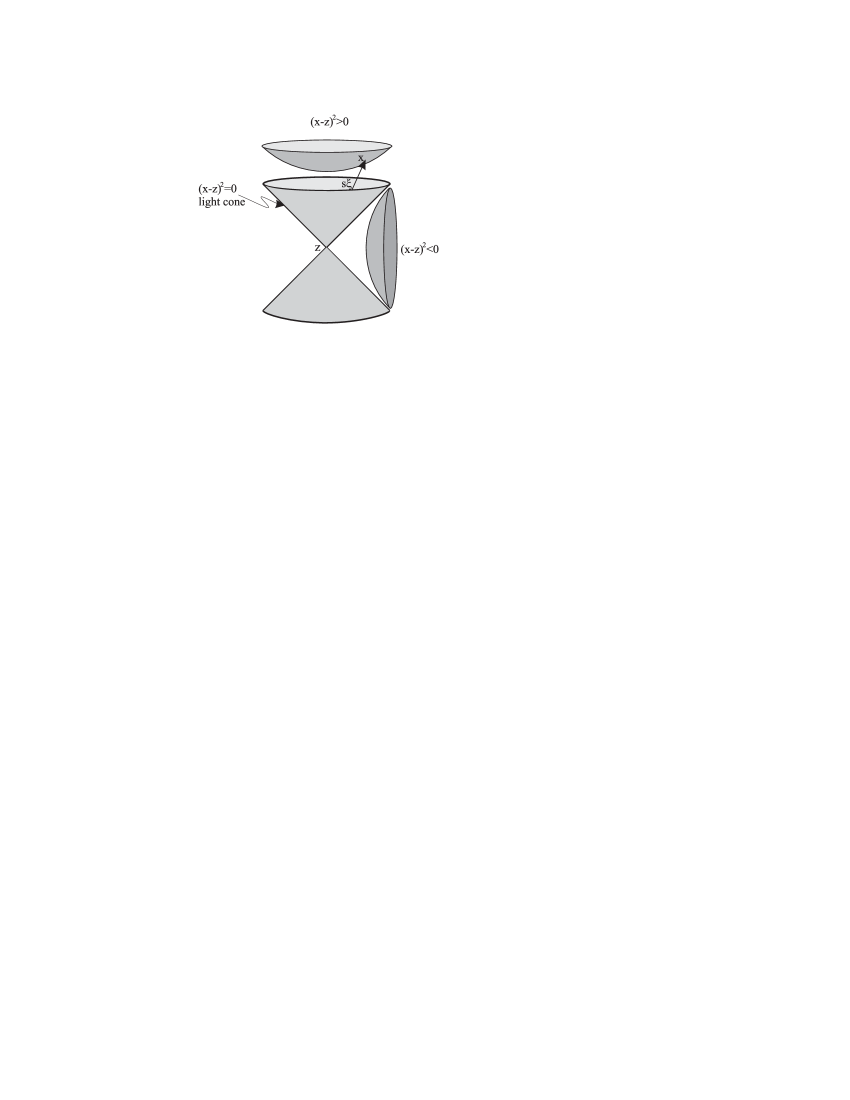
Figure IV.1. Geometrical setting. The point $z$ is fixed, and there the initial condition is specified. The parametrix fulfills the wave equation in the variable $x$.

IV.1. Scalar field case

Before we concentrate on the Dirac field, let us look for the fundamental solutions of the scalar wave operator

$$\left[\Box^{x}+B^{a}(x)\partial^{x}_{a}+c(x)\right]\varphi(x,z)=\mathcal{D}_{x}\ \varphi(x,z)=0.$$ (IV.1)

If the functions $B^{a}(x),\ c(x)$ exhibit little or no symmetry, then it is difficult to find the fundamental solutions explicitly. We shall present here a method of Hadamard which allows us to find approximate fundamental solutions of the wave equations. They are approximate in the sense that

• they differ from the exact fundamental solutions by a residual term which is differentiable up to an arbitrarily high order,

• the differential operator $\mathcal{D}_{x}$ acting on the residual term of order $N$ gives a distribution which vanishes as $\Gamma^{N}$ with $\Gamma\rightarrow 0$.

IV.1.1. Progressing wave expansion

In order to find approximate fundamental solutions we use the method called ’the progressing wave expansion’. The solutions of order $N$ will be parameterized as follows:

$$\varphi(x)=\sum_{n=0}^{N}U_{n}(x)\cdot S_{n}[\chi(x)],$$

where $U_{n}(x)$ are $\mathcal{C}^{\infty}$ amplitudes, $S_{n}$ are distributions of one variable called the wave forms, and $\chi$ is a smooth function, the phase. Any discontinuity of $\varphi$ comes from the distributions $S_{n}$, and thus surfaces of constant phase are possible surfaces of discontinuity.

It is clear from the outset that the progressing wave expansion introduces a considerable redundancy. Not only it is possible to describe different types of singular solutions of the wave equations (with different surfaces of singularity), but also the same solutions may be expressed in different ways.

We use this redundancy in order to specify the concrete situation (we look for a singularity on the light cone $\Gamma=0$) and to simplify the search for the amplitudes. In the construction we fix from the beginning the wave forms $S_{n}$ and the phase function and ask, whether it is possible to choose the amplitudes so that the distribution $\varphi$ fulfills the wave equation.

The wave operator $\mathcal{D}$ has the same principal symbol as $\Box_{x}$; because of that it will turn out advantageous to require the wave forms to fulfill

$$\frac{dS_{n}}{d\Gamma}=S_{n-1}.$$

Moreover, if we choose the phase function to be equal to the square geodesic distance between $x$ and some fixed basis point $z$, an additional equation between the wave forms must be fulfilled:

$$\Gamma S_{-2}(\Gamma)+2S_{-1}(\Gamma)=0,$$ (IV.2)

for otherwise no choice of amplitudes can lead to a solution of the wave equation.

If we choose a set of wave forms $S_{n}$ which fulfill both equations and if we find for this set the amplitudes $U_{n}(x)$ (which we will do in the subsequent sections), then the problem of finding $\varphi$ is solved by means of a series (of progressing waves).

The equation (IV.2) prescribes the degree of homogeneity of $S_{-1}$. Formally, the following distributions fulfill this requirement:

$$S_{0} =\frac{1}{\Gamma} \mbox{or}\qquad S_{0} =\delta(\Gamma).$$

Irrespective of this choice and also of the choice of the regularization of $\Gamma$, the method of progressing waves will yield the same amplitude functions. For instance, the retarded and advanced solutions as well as the Feynman parametrix have the same progressing wave amplitudes and differ only by the wave forms.

From now on we shall concentrate on

$$S_{0}(\Gamma) =1/\Gamma,$$

$$S_{1}(\Gamma) =\ln\Gamma.$$

In this case the progressing wave expansion coincides with the ansatz of [DB60] which will be later recognized as the universal form of the singularity of the two-point function of the quantum Dirac field (the Hadamard form):

$$\varphi(x,z)=\frac{u(x,z)}{\Gamma}+v(x,z)\ln(\Gamma)+w(x,z),$$ (IV.3)

where $v$ and $w$ are sums of higher order wave forms and their coefficients:

$$v =v_{0}(x,z)+v_{1}(x,z)\Gamma+v_{2}(x,z)\Gamma^{2}+\ldots,$$

$$w =w_{0}(x,z)+w_{1}(x,z)\Gamma+w_{2}(x,z)\Gamma^{2}+\ldots.$$

The amplitude functions $u,v_{n},w_{n}$ will be constructed locally (in the smallest causal normal neighborhood containing $x$ and $z$) and will fulfill a set of (first-order differential) transport equations.

IV.1.2. Regularization of the phase function

In the method of progressing waves the wave forms were distributions of one variable taking as an argument the value of the phase function $\chi(x)$. Such a composition should be a distribution on the space of spacetime-valued test functions. Its action on $g\in\mathcal{C}_{0}^{\infty}(\mathbb{R}^{4})$ can be obtained from

$$\langle S[\chi],g\rangle=\int d\tau\ S(\tau)\delta[\tau-\chi(x)]\ g(x)\ d^{4}x.$$

The operation is justified, only if the integration over $d^{4}x$ yields a smooth function of compact support in $\tau$. This point is in general non-trivial. A detailed investigation reported in [Fri74] section 2.9 assures that, as long as $\chi(x)$ is smooth and the gradient of $\chi$ is non-vanishing, the function

$$f(\tau)=\int\delta[\chi(x)-\tau]\phi(x)\ d^{4}x$$

is indeed a $\mathcal{C}_{0}^{\infty}(\mathbb{R})$ function for all test functions $\phi\in\mathcal{C}_{0}^{\infty}(\mathbb{R}^{4})$ so that the composite distributions $S=S[\chi(x)]$ are well-defined. The phase function $\chi(x)=\Gamma$, however, possesses a vanishing gradient at the origin $x=z$ (for $\Gamma=0$), and so it is not directly suitable for the method of progressing waves, although we know from simple examples that the fundamental solutions of the wave equations are precisely singular solutions whose singularities lie on the light cone $\Gamma=0$. One finds them with the help of the Fourier transform. There the transformed fundamental solution (eg. of the d’Alembert operator) $\hat{H}(p)$ fulfills

$$\mathcal{D}(p)\hat{H}(p)=e^{ipy}.$$

The inverse of $\mathcal{D}(p)$ has a nontrivial manifold of zeros which makes $H(p)$ not locally integrable. Such expressions have to be regularized. There are different possibilities of defining the inverse, and they lead to different distributions; as we know, there are different fundamental solutions of the d’Alembert equation.

In the case at hand we regularize the phase function $\chi=\Gamma$ by means of a weak limit $i\epsilon\rightarrow 0$. Specifically, we define

$$\Gamma_{\epsilon} =(x_{0}-z_{0}+i\epsilon)^{2}-({\mathbf{x}}-{\mathbf{z}})^{2},$$

$$\Gamma_{F} =(x_{0}-z_{0})^{2}-({\mathbf{x}}-{\mathbf{z}})^{2}+i\epsilon.$$

Both the above regularizations of $\chi(x,z)=\Gamma$ and the distributions of them coincide, if the test functions with which they are integrated are not supported at the origin.

As is the case with momentum space regularizations of $1/p^{2}$ which have very different properties in the coordinate space (eg. retarded vs. advanced solution), different regularizations of $\Gamma$ have different properties in momentum space. Regarded as distributions of both arguments, $x$ and $z$, they have different wave front sets.

The regularization of the distribution at the origin does not alter its homogeneity and therefore all regularizations of $\delta(\Gamma)$ and $1/\Gamma$ fulfill (IV.2). All their progressing wave amplitudes are therefore the same.

IV.1.3. Construction of the parametrix; the transport equations

Consider the wave equation $\mathcal{D}_{x}\varphi(x,z)=0$ together with the particular progressing wave expansion (taken with some regularization of $\Gamma$):

$$\varphi(x,z)=\frac{u(x,z)}{\Gamma}+v(x,z)\ln\Gamma+w(x,z),$$ (IV.4)

where the smooth functions $v$, $w$ are given by the power series:

$$v(x,z) =\sum_{n=0}^{\infty}v_{n}(x,z)\ \Gamma^{n},$$

$$w(x,z) =\sum_{n=1}^{\infty}w_{n}(x,z)\ \Gamma^{n}.$$

The method of progressing waves is a way to find fundamental solutions which are singular. There always exists a possibility of adding a smooth solution of the wave equation to $\varphi$. This freedom is expressed here as a freedom to choose an arbitrary, smooth amplitude $w_{0}(x,z)$ which (as we shall see in the moment) influences all the $w_{n}(x,z)$, $n>0$.

With

$$\partial^{x}_{a}\Gamma =2(x-z)_{a}=s\xi_{a},$$

$$\partial^{a}\Gamma\partial_{a}\Gamma =4\Gamma,$$

$$\Box^{x}\Gamma =8,$$

we find

$$\partial_{a}\varphi=-\frac{u}{\Gamma^{2}}\ \partial_{a}\Gamma+\frac{1}{\Gamma}\ \partial_{a}u+\partial_{a}\Gamma\sum^{\infty}_{0}v_{n}\Gamma^{n-1}+\ln\Gamma\left(\partial_{a}\Gamma\sum^{\infty}_{1}n\ v_{n}\Gamma^{n-1}+\sum^{\infty}_{0}\partial_{a}v_{n}\ \Gamma^{n}\right)\\ +\sum^{\infty}_{1}\left(\partial_{a}w_{n}\ \Gamma^{n}+\partial_{a}\Gamma\ n\ w_{n}\Gamma^{n-1}\right),$$

where all the differentiations are executed with respect to $x$, the variable $z$ being merely a parameter. We also find

$$\Box\varphi=\frac{1}{\Gamma^{2}}\ (-2\ \partial_{a}\Gamma\partial^{a}u)+\Box u\frac{1}{\Gamma}+8v_{0}\frac{1}{\Gamma}+8\sum^{\infty}_{1}v_{n}\Gamma^{n-1}+\partial_{a}\Gamma\partial^{a}v_{0}\frac{1}{\Gamma}+\partial_{a}\Gamma\sum^{\infty}_{1}\partial^{a}v_{n}\Gamma^{n-1}+\\ -4v_{0}\frac{1}{\Gamma}+4\sum^{\infty}_{1}(n-1)\ v_{n}\Gamma^{n-1}+\partial^{a}\Gamma\partial_{a}v_{0}\frac{1}{\Gamma}+\partial^{a}\Gamma\sum^{\infty}_{1}\partial_{a}v_{n}\ \Gamma^{n-1}+4\sum^{\infty}_{1}n\ v_{n}\Gamma^{n-1}+\\ +\ln\Gamma\left[8\sum^{\infty}_{1}n\ v_{n}\Gamma^{n-1}+\partial_{a}\Gamma\sum^{\infty}_{1}n\ \partial^{a}v_{n}\ \Gamma^{n-1}+4\sum^{\infty}_{1}n(n-1)\ v_{n}\Gamma^{n-1}+\sum^{\infty}_{0}\Box v_{n}\ \Gamma^{n}+\right.\\ +\left.\partial^{a}\Gamma\sum^{\infty}_{1}n\ \partial_{a}v_{n}\ \Gamma^{n-1}\right]+\sum^{\infty}_{1}\left[\Box w_{n}\ \Gamma^{n}+2n\ \partial^{a}\Gamma\partial_{a}w_{n}\ \Gamma^{n-1}+4n(n-1)\ w_{n}\Gamma^{n-1}+8n\ w_{n}\Gamma^{n-1}\right].$$

Ordering the above expression so that appropriate progressing waves appear together, we find:

$$\Box\varphi=\frac{1}{\Gamma^{2}}(-2\partial^{a}\Gamma\partial_{a}u)+\frac{1}{\Gamma}\left(\Box u+4v_{0}+2\partial^{a}\Gamma\partial_{a}v_{0}\right)+\\ +\sum^{\infty}_{0}\ln\Gamma\ \Gamma^{n}\left[2(n+1)\ \partial^{a}\Gamma\partial_{a}v_{n+1}+4(n+1)(n+2)\ v_{n+1}+\Box v_{n}\right]+\\ +\sum^{\infty}_{0}\Gamma^{n}\left[2\ \partial^{a}\Gamma\partial_{a}v_{n+1}+4(2n+3)\ v_{n+1}+2(n+1)\ \partial^{a}\Gamma\partial_{a}w_{n+1}+4(n+1)(n+2)\ w_{n+1}+\Box w_{n}\right],$$

(we have set $w_{0}=0$). Finally, by setting all the coefficients in front of the factors $\Gamma^{n}$ and $\Gamma^{n}\ln\Gamma$ to zero, we obtain the following system of differential equations of first order for $u,v_{0}$ and $v_{n},w_{n}$:

$$2\ \partial^{a}\Gamma\partial_{a}u+uB^{a}\partial_{a}\Gamma =0, 2\ \partial^{a}\Gamma\partial_{a}v_{0}+v_{0}(4+B^{a}\partial_{a}\Gamma) =-\mathcal{D}_{x}u, 2\ \partial^{a}\Gamma\partial_{a}v_{n}+v_{n}\left[4(n+1)+B^{a}\partial_{a}\Gamma\right] =-\frac{1}{n}\mathcal{D}_{x}v_{n-1},$$ (IV.5a) (IV.5b) (IV.5c)

and

$$2\ \partial^{a}\Gamma\partial_{a}w_{n}+w_{n}[4(n+1)+B^{a}\partial_{a}\Gamma]=\\ -\frac{1}{n}\left\{v_{n}[4(2n+1)+B^{a}\partial_{a}\Gamma]+2\partial^{a}\Gamma\partial_{a}v_{n}+\mathcal{D}_{x}w_{n-1}\right\}.$$ (IV.5d)

This is a system of partial differential equations. If we recognize that the contractions of the partial derivatives on the left-hand side can be written as derivatives along the geodesic, $\tfrac{d}{ds}$,

$$\partial^{a}\Gamma\partial_{a}f=2s\xi^{a}\partial_{a}f=2s\frac{df}{ds},$$

we realize that we are dealing with a recursive system of ordinary differential equations. They will be solved in the following order: first $u$, then $v_{n}$ with growing $n$, and finally $w_{n}$. At each step we have an ordinary differential equation to solve, yet the whole system is a system of partial differential equations, because the knowledge of all the previous amplitudes in the neighborhood of the geodesic (there are normal derivatives in $\mathcal{D}$) is necessary in order to establish the equation for the next amplitude.

Apart from the ambiguity of choosing $w_{0}$, the system has a unique smooth solution with initial condition $u(z,z)=1$. Setting the function $u$ equal to $1$ on the diagonal $x=z$ and demanding the smoothness of $v_{0},v_{n},w_{n}$ determines these functions uniquely. The proof of the above statement will be apparent from the construction which follows. The role of smoothness as an initial condition is the following: the derivatives with respect to $s$ are all multiplied by $s$ and therefore have to vanish at $s=0$, if we want the solutions to be smooth. The transport equations themselves taken at $s=0$ give us the initial conditions for $v_{0},v_{n}$ and $w_{n}$ in a recursive manner.

IV.1.4. Solution of the transport equations

The system of differential equations from the previous section will now be solved constructively.

Equation for $u(z,x)$:
This equation allows us to find a smooth coefficient $u(z,x)$, i.e. the coefficient which appears in front of the most singular term in the parametrix (IV.4) with appropriate initial condition $u(z,z)=1$. Due to $\partial_{a}\Gamma=2s\xi_{a}$, we find

$$u=\exp\left[-\frac{1}{2}\int_{0}^{s}B^{a}\xi_{a}\ d\tau\right],$$

where only $B^{a}$ is $\tau$-dependent. It is important to realize that the above solution is smooth in the limit $s\rightarrow 0$.

Equation for $v_{0}(z,x)$:
The equation (IV.5b) for $v_{0}$ may be integrated as soon as the function $u(z,x)$ is already known. We find

$$v_{0}=-\frac{u}{4s}\int_{0}^{s}\frac{\mathcal{D}_{x}u}{u}[\tau]\ d\tau$$

which is a smooth function if $u(x,z)$ is smooth.

Equations for $v_{n}(z,x)$:
In order to find smooth solutions of (IV.5c) one proceeds recursively. Here we shall present the typical method of finding such solutions in a compact form. Noting that

$$B^{a}\partial_{a}\Gamma=-\frac{1}{u}2\ \partial^{a}\Gamma\partial_{a}u=-4s\ \frac{1}{u}\frac{du}{ds},$$

it is possible to transform (IV.5c) into

$$4s\frac{d}{ds}\left(\frac{v_{n}}{u}\right)+4(n+1)\frac{v_{n}}{u}=-\frac{\mathcal{D}_{x}v_{n-1}}{n\cdot u}$$

and then to obtain straightforwardly,

$$v_{n}=-\frac{u}{4s^{n+1}}\int_{0}^{s}\tau^{n}\ \frac{\mathcal{D}_{x}v_{n-1}}{n\cdot u}\ d\tau.$$

The function $v_{n}(x,z)$ is smooth, if $v_{n-1}$ is also smooth.

Equations for $w_{n}(z,x)$:
The equations (IV.5d) can be solved similarly. According to (IV.5c) the RHS of (IV.5d) can be transformed into

$$RHS_{\text{\eqref{rown_wn}}}=\frac{\mathcal{D}_{x}v_{n-1}}{n^{2}}-4v_{n}-\frac{1}{n}\mathcal{D}_{x}w_{n-1}.$$

Analogously to the $v_{n}$-case one finds:

$$w_{n}=-\frac{u}{4s^{n+1}}\int_{0}^{s}\tau^{n}\ \left(-\frac{\mathcal{D}_{x}v_{n-1}}{n^{2}}+\frac{\mathcal{D}_{x}w_{n-1}}{n}+4v_{n}\right)\ d\tau.$$

Remark.

It is perhaps valuable to note that all the coefficients, $u(x,z),\ v_{n}(x,z),\ w_{n}(x,z)$, are functionals of the external field. Moreover, what counts is the external field in an infinitesimal neighborhood of the geodesic (straight line) which connects $x$ and $z$. Due to the powers of $s$ in the denominator, however, those functionals do not vanish in the limit $s\rightarrow 0$; they rather have a form of certain averages of the external field on the line $x-z$.

IV.2. Dirac field

Now we shall consider the case of a free Dirac field propagating in a given, fixed electromagnetic environment. Our goal is to find the parametrix exactly the way we did in the last section in the scalar case. By doing so, we shall also investigate the transport equations for the expansion coefficients in much greater detail, in part because the Dirac parametrix will be relied on this thesis.

We consider the Dirac equation:

$$i\gamma^{a}[\partial_{a}-ieA_{a}(x)]H(x,z)-mH(x,z)\equiv\mathchoice{D_{\kern 0.0pt\hbox{$\scriptstyle xA\hbox{}$}}^{\hbox{$\scriptstyle{}$}\kern 0.0pt\hbox{$\kern 0.0pt\scriptstyle\hbox{}\hbox{}C$}}}{D_{\kern 0.0pt\hbox{$\scriptstyle xA\hbox{}$}}^{\hbox{$\scriptstyle{}$}\kern 0.0pt\hbox{$\kern 0.0pt\scriptstyle\hbox{}\hbox{}C$}}}{D_{\kern 0.0pt\hbox{$\scriptscriptstyle xA\hbox{}$}}^{\hbox{$\scriptscriptstyle{}$}\kern 0.0pt\hbox{$\kern 0.0pt\scriptscriptstyle\hbox{}\hbox{}C$}}}{D_{\kern 0.0pt\hbox{$\scriptscriptstyle xA\hbox{}$}}^{\hbox{$\scriptscriptstyle{}$}\kern 0.0pt\hbox{$\kern 0.0pt\scriptscriptstyle\hbox{}\hbox{}C$}}}H_{CB}(x,z)=0,$$ (IV.6)

where we have emphasized the bi-spinorial character of $H(x,z)$. We define also an auxiliary differential operator,

$$\hat{D}_{x}=i\gamma^{a}\partial_{a}+e\gamma^{a}A_{a}(x)+m,$$ (IV.7)

and make use of a standard ansatz, namely, the parametrix of the Dirac equation (IV.6) is given by

$$H_{AB}(x,z)=\hat{D}\mathchoice{\,{}_{\kern 0.0pt\hbox{$\scriptstyle xA\hbox{}$}}^{\hbox{$\scriptstyle{}$}\kern 0.0pt\hbox{$\kern 0.0pt\scriptstyle\hbox{}C$}}}{\,{}_{\kern 0.0pt\hbox{$\scriptstyle xA\hbox{}$}}^{\hbox{$\scriptstyle{}$}\kern 0.0pt\hbox{$\kern 0.0pt\scriptstyle\hbox{}C$}}}{\,{}_{\kern 0.0pt\hbox{$\scriptscriptstyle xA\hbox{}$}}^{\hbox{$\scriptscriptstyle{}$}\kern 0.0pt\hbox{$\kern 0.0pt\scriptscriptstyle\hbox{}C$}}}{\,{}_{\kern 0.0pt\hbox{$\scriptscriptstyle xA\hbox{}$}}^{\hbox{$\scriptscriptstyle{}$}\kern 0.0pt\hbox{$\kern 0.0pt\scriptscriptstyle\hbox{}C$}}}\ \phi_{CB}(x,z),$$ (IV.8)

where $\phi(x,z)$ is the (bi-spinorial) parametrix fulfilling the following second order partial differential equation:

$$\mathcal{D}\phi\equiv D\hat{D}\phi=[i(\partial/-ieA/)-m][i(\partial/-ieA/)+m]\phi=0$$

modulo smooth terms; here

$$\mathcal{D}=[\Box-2ie\ A^{a}\partial_{a}+m^{2}+e^{2}A^{2}]\cdot\mathchoice{\delta_{\kern 0.0pt\hbox{$\scriptstyle\hbox{}B$}}^{\hbox{$\scriptstyle{}$}\kern 0.0pt\hbox{$\kern 0.0pt\scriptstyle A\hbox{}$}}}{\delta_{\kern 0.0pt\hbox{$\scriptstyle\hbox{}B$}}^{\hbox{$\scriptstyle{}$}\kern 0.0pt\hbox{$\kern 0.0pt\scriptstyle A\hbox{}$}}}{\delta_{\kern 0.0pt\hbox{$\scriptscriptstyle\hbox{}B$}}^{\hbox{$\scriptscriptstyle{}$}\kern 0.0pt\hbox{$\kern 0.0pt\scriptscriptstyle A\hbox{}$}}}{\delta_{\kern 0.0pt\hbox{$\scriptscriptstyle\hbox{}B$}}^{\hbox{$\scriptscriptstyle{}$}\kern 0.0pt\hbox{$\kern 0.0pt\scriptscriptstyle A\hbox{}$}}}-\frac{ie}{2}(\gamma^{a}\gamma^{b}-\gamma^{b}\gamma^{a})\mathchoice{\,{}_{\kern 0.0pt\hbox{$\scriptstyle\hbox{}B$}}^{\hbox{$\scriptstyle{}$}\kern 0.0pt\hbox{$\kern 0.0pt\scriptstyle A\hbox{}$}}}{\,{}_{\kern 0.0pt\hbox{$\scriptstyle\hbox{}B$}}^{\hbox{$\scriptstyle{}$}\kern 0.0pt\hbox{$\kern 0.0pt\scriptstyle A\hbox{}$}}}{\,{}_{\kern 0.0pt\hbox{$\scriptscriptstyle\hbox{}B$}}^{\hbox{$\scriptscriptstyle{}$}\kern 0.0pt\hbox{$\kern 0.0pt\scriptscriptstyle A\hbox{}$}}}{\,{}_{\kern 0.0pt\hbox{$\scriptscriptstyle\hbox{}B$}}^{\hbox{$\scriptscriptstyle{}$}\kern 0.0pt\hbox{$\kern 0.0pt\scriptscriptstyle A\hbox{}$}}}\partial_{a}A_{b}$$ (IV.9)

is the spinorial differential operator which acts on the $x$-variable (and its spinorial index ”$A$”). From now on the external electromagnetic field is considered to be in the Lorentz gauge $\partial A=0$. Making use of the definition $\tfrac{1}{2}[\gamma^{a},\gamma^{b}]=\sigma^{ab}$ we obtain

$$\mathcal{D}=[\Box-2ie\ A^{a}\partial_{a}+m^{2}+e^{2}A^{2}]\cdot\mathchoice{\delta_{\kern 0.0pt\hbox{$\scriptstyle\hbox{}B$}}^{\hbox{$\scriptstyle{}$}\kern 0.0pt\hbox{$\kern 0.0pt\scriptstyle A\hbox{}$}}}{\delta_{\kern 0.0pt\hbox{$\scriptstyle\hbox{}B$}}^{\hbox{$\scriptstyle{}$}\kern 0.0pt\hbox{$\kern 0.0pt\scriptstyle A\hbox{}$}}}{\delta_{\kern 0.0pt\hbox{$\scriptscriptstyle\hbox{}B$}}^{\hbox{$\scriptscriptstyle{}$}\kern 0.0pt\hbox{$\kern 0.0pt\scriptscriptstyle A\hbox{}$}}}{\delta_{\kern 0.0pt\hbox{$\scriptscriptstyle\hbox{}B$}}^{\hbox{$\scriptscriptstyle{}$}\kern 0.0pt\hbox{$\kern 0.0pt\scriptscriptstyle A\hbox{}$}}}-\frac{e}{2}\ \mathchoice{\sigma_{\kern 0.0pt\hbox{$\scriptstyle\hbox{}\hbox{}B$}}^{\hbox{$\scriptstyle{}$}\kern 0.0pt\hbox{$\kern 0.0pt\scriptstyle abA\hbox{}$}}}{\sigma_{\kern 0.0pt\hbox{$\scriptstyle\hbox{}\hbox{}B$}}^{\hbox{$\scriptstyle{}$}\kern 0.0pt\hbox{$\kern 0.0pt\scriptstyle abA\hbox{}$}}}{\sigma_{\kern 0.0pt\hbox{$\scriptscriptstyle\hbox{}\hbox{}B$}}^{\hbox{$\scriptscriptstyle{}$}\kern 0.0pt\hbox{$\kern 0.0pt\scriptscriptstyle abA\hbox{}$}}}{\sigma_{\kern 0.0pt\hbox{$\scriptscriptstyle\hbox{}\hbox{}B$}}^{\hbox{$\scriptscriptstyle{}$}\kern 0.0pt\hbox{$\kern 0.0pt\scriptscriptstyle abA\hbox{}$}}}\ F_{ab}.$$

Now we introduce certain abbreviations which will make the following considerations much more apparent:

$$\mathcal{D}=[\Box+B^{a}(x)\partial_{a}+c(x)]\cdot\mathchoice{\delta_{\kern 0.0pt\hbox{$\scriptstyle\hbox{}B$}}^{\hbox{$\scriptstyle{}$}\kern 0.0pt\hbox{$\kern 0.0pt\scriptstyle A\hbox{}$}}}{\delta_{\kern 0.0pt\hbox{$\scriptstyle\hbox{}B$}}^{\hbox{$\scriptstyle{}$}\kern 0.0pt\hbox{$\kern 0.0pt\scriptstyle A\hbox{}$}}}{\delta_{\kern 0.0pt\hbox{$\scriptscriptstyle\hbox{}B$}}^{\hbox{$\scriptscriptstyle{}$}\kern 0.0pt\hbox{$\kern 0.0pt\scriptscriptstyle A\hbox{}$}}}{\delta_{\kern 0.0pt\hbox{$\scriptscriptstyle\hbox{}B$}}^{\hbox{$\scriptscriptstyle{}$}\kern 0.0pt\hbox{$\kern 0.0pt\scriptscriptstyle A\hbox{}$}}}-\frac{e}{2}\mathchoice{\sigma_{\kern 0.0pt\hbox{$\scriptstyle\hbox{}\hbox{}\hbox{}B$}}^{\hbox{$\scriptstyle{}$}\kern 0.0pt\hbox{$\kern 0.0pt\scriptstyle abA\hbox{}$}}}{\sigma_{\kern 0.0pt\hbox{$\scriptstyle\hbox{}\hbox{}\hbox{}B$}}^{\hbox{$\scriptstyle{}$}\kern 0.0pt\hbox{$\kern 0.0pt\scriptstyle abA\hbox{}$}}}{\sigma_{\kern 0.0pt\hbox{$\scriptscriptstyle\hbox{}\hbox{}\hbox{}B$}}^{\hbox{$\scriptscriptstyle{}$}\kern 0.0pt\hbox{$\kern 0.0pt\scriptscriptstyle abA\hbox{}$}}}{\sigma_{\kern 0.0pt\hbox{$\scriptscriptstyle\hbox{}\hbox{}\hbox{}B$}}^{\hbox{$\scriptscriptstyle{}$}\kern 0.0pt\hbox{$\kern 0.0pt\scriptscriptstyle abA\hbox{}$}}}\ F_{ab}(x),$$ (IV.10)

where

$$B^{a}(x) =-2ieA^{a}(x),$$

$$c(x) =m^{2}+e^{2}A^{a}(x)A_{a}(x),$$

and so the Lorentz gauge condition reads: $\partial_{a}B^{a}=0$.

Clearly the operator (IV.10) differs from the scalar operator considered in the previous section. Although the first part of it is multiplied with a spinorial delta $\mathchoice{\delta_{\kern 0.0pt\hbox{$\scriptstyle\hbox{}B$}}^{\hbox{$\scriptstyle{}$}\kern 0.0pt\hbox{$\kern 0.0pt\scriptstyle A\hbox{}$}}}{\delta_{\kern 0.0pt\hbox{$\scriptstyle\hbox{}B$}}^{\hbox{$\scriptstyle{}$}\kern 0.0pt\hbox{$\kern 0.0pt\scriptstyle A\hbox{}$}}}{\delta_{\kern 0.0pt\hbox{$\scriptscriptstyle\hbox{}B$}}^{\hbox{$\scriptscriptstyle{}$}\kern 0.0pt\hbox{$\kern 0.0pt\scriptscriptstyle A\hbox{}$}}}{\delta_{\kern 0.0pt\hbox{$\scriptscriptstyle\hbox{}B$}}^{\hbox{$\scriptscriptstyle{}$}\kern 0.0pt\hbox{$\kern 0.0pt\scriptscriptstyle A\hbox{}$}}}$, i.e. effectively acts as a scalar operator , the second part (which does not contain any differentiation) contains a term $\mathchoice{\sigma_{\kern 0.0pt\hbox{$\scriptstyle\hbox{}\hbox{}\hbox{}B$}}^{\hbox{$\scriptstyle{}$}\kern 0.0pt\hbox{$\kern 0.0pt\scriptstyle abA\hbox{}$}}}{\sigma_{\kern 0.0pt\hbox{$\scriptstyle\hbox{}\hbox{}\hbox{}B$}}^{\hbox{$\scriptstyle{}$}\kern 0.0pt\hbox{$\kern 0.0pt\scriptstyle abA\hbox{}$}}}{\sigma_{\kern 0.0pt\hbox{$\scriptscriptstyle\hbox{}\hbox{}\hbox{}B$}}^{\hbox{$\scriptscriptstyle{}$}\kern 0.0pt\hbox{$\kern 0.0pt\scriptscriptstyle abA\hbox{}$}}}{\sigma_{\kern 0.0pt\hbox{$\scriptscriptstyle\hbox{}\hbox{}\hbox{}B$}}^{\hbox{$\scriptscriptstyle{}$}\kern 0.0pt\hbox{$\kern 0.0pt\scriptscriptstyle abA\hbox{}$}}}$ which mixes spinorial indices. In other words, it is only because of the second term that we have to consider the spinorial character of the expansion coefficients.

The bi-spinorial parametrix will be found with the help of the progressing waves. The issue to be investigated throughout this section is the gauge covariance of the system of the transport equations. They are:

$\displaystyle s\ \xi^{a}(\partial_{a}-ieA_{a})_{x}\ u(x,z)$ $\displaystyle=0,$ $\displaystyle s\ \xi^{a}(\partial_{a}-ieA_{a})_{x}\ v_{0}(x,z)+v_{0}(x,z)$ $\displaystyle=-\frac{1}{4}\mathcal{D}_{x}u(x,z),$ $\displaystyle s\ \xi^{a}(\partial_{a}-ieA_{a})_{x}\ v_{n}(x,z)+(n+1)v_{n}(x,z)$ $\displaystyle=-\frac{\mathcal{D}_{x}v_{n-1}(x,z)}{4n},$

and

$$s\ \xi^{a}(\partial_{a}-ieA_{a})_{x}\ w_{n}(x,z)+(n+1)w_{n}(x,z)=\\ -\frac{1}{n}\left[s\ \xi^{a}(\partial_{a}-ieA_{a})_{x}\ v_{n}(x,z)+(2n+1)v_{n}(x,z)+\frac{\mathcal{D}_{x}}{4}\ w_{n-1}(x,z)\right].$$

By writing the transport equations in this way, we have illuminated their covariance w.r.t. the gauge transformations, namely, if the external field is changed by

$$A_{a}^{\prime}=A_{a}+\partial_{a}\Lambda,$$

then the primed coefficients of the Hadamard expansion are related to the initial ones by

$$u^{\prime}(x)=e^{ie\Lambda(x)}u(x)$$

and fulfill the (primed) transport equations.

A couple of general remarks about the system of differential equations for the parametrix coefficients are in order. Firstly, they are supplied with only one boundary condition $u(z,z)=1$ (times the identity matrix). All the boundary conditions for $v_{n}$ are to be derived recursively from the condition that they remain finite as $s\rightarrow 0$. This is only possible because $s=0$ is the singular point of each of those equations. Secondly, there is an impression that we deal with ordinary differential equations. Indeed, as the geodesic tangent vector $\xi$ is fixed, at least the homogeneous (i.e. LHS) part of those equations contains only derivatives w.r.t. the geodesic distance $s$. However, the RHS, in particular the operator $\mathcal{D}_{x}$ contains also derivatives in directions orthogonal to $\xi$. As a consequence the expansion coefficients $v_{n}(x,z)$ depend not only on the external field on the geodesic which joins $x$ and $z$, but also on its values in an arbitrarily small neighborhood of this geodesic. The third important issue is the dependence of the coefficients on $z$. Up to now $z$ was regarded as ”origin” of the expansion and played no active role. However, we may pose the boundary value problem at a different point, say $\tilde{z}$, and ask to compare the expansion coefficients $v(x,z)$ and $v(x,\tilde{z})$. We shall investigate this issue in a separate section (IV.4).

The equation for $\mathchoice{u_{\kern 0.0pt\hbox{$\scriptstyle\hbox{}B$}}^{\hbox{$\scriptstyle{}$}\kern 0.0pt\hbox{$\kern 0.0pt\scriptstyle A\hbox{}$}}}{u_{\kern 0.0pt\hbox{$\scriptstyle\hbox{}B$}}^{\hbox{$\scriptstyle{}$}\kern 0.0pt\hbox{$\kern 0.0pt\scriptstyle A\hbox{}$}}}{u_{\kern 0.0pt\hbox{$\scriptscriptstyle\hbox{}B$}}^{\hbox{$\scriptscriptstyle{}$}\kern 0.0pt\hbox{$\kern 0.0pt\scriptscriptstyle A\hbox{}$}}}{u_{\kern 0.0pt\hbox{$\scriptscriptstyle\hbox{}B$}}^{\hbox{$\scriptscriptstyle{}$}\kern 0.0pt\hbox{$\kern 0.0pt\scriptscriptstyle A\hbox{}$}}}(x,z)$ reads

$$\frac{d}{ds}\mathchoice{u_{\kern 0.0pt\hbox{$\scriptstyle\hbox{}B$}}^{\hbox{$\scriptstyle{}$}\kern 0.0pt\hbox{$\kern 0.0pt\scriptstyle A\hbox{}$}}}{u_{\kern 0.0pt\hbox{$\scriptstyle\hbox{}B$}}^{\hbox{$\scriptstyle{}$}\kern 0.0pt\hbox{$\kern 0.0pt\scriptstyle A\hbox{}$}}}{u_{\kern 0.0pt\hbox{$\scriptscriptstyle\hbox{}B$}}^{\hbox{$\scriptscriptstyle{}$}\kern 0.0pt\hbox{$\kern 0.0pt\scriptscriptstyle A\hbox{}$}}}{u_{\kern 0.0pt\hbox{$\scriptscriptstyle\hbox{}B$}}^{\hbox{$\scriptscriptstyle{}$}\kern 0.0pt\hbox{$\kern 0.0pt\scriptscriptstyle A\hbox{}$}}}=ieA^{a}\xi_{a}\ \mathchoice{u_{\kern 0.0pt\hbox{$\scriptstyle\hbox{}B$}}^{\hbox{$\scriptstyle{}$}\kern 0.0pt\hbox{$\kern 0.0pt\scriptstyle A\hbox{}$}}}{u_{\kern 0.0pt\hbox{$\scriptstyle\hbox{}B$}}^{\hbox{$\scriptstyle{}$}\kern 0.0pt\hbox{$\kern 0.0pt\scriptstyle A\hbox{}$}}}{u_{\kern 0.0pt\hbox{$\scriptscriptstyle\hbox{}B$}}^{\hbox{$\scriptscriptstyle{}$}\kern 0.0pt\hbox{$\kern 0.0pt\scriptscriptstyle A\hbox{}$}}}{u_{\kern 0.0pt\hbox{$\scriptscriptstyle\hbox{}B$}}^{\hbox{$\scriptscriptstyle{}$}\kern 0.0pt\hbox{$\kern 0.0pt\scriptscriptstyle A\hbox{}$}}}$$

with the initial condition $\mathchoice{u_{\kern 0.0pt\hbox{$\scriptstyle\hbox{}B$}}^{\hbox{$\scriptstyle{}$}\kern 0.0pt\hbox{$\kern 0.0pt\scriptstyle A\hbox{}$}}}{u_{\kern 0.0pt\hbox{$\scriptstyle\hbox{}B$}}^{\hbox{$\scriptstyle{}$}\kern 0.0pt\hbox{$\kern 0.0pt\scriptstyle A\hbox{}$}}}{u_{\kern 0.0pt\hbox{$\scriptscriptstyle\hbox{}B$}}^{\hbox{$\scriptscriptstyle{}$}\kern 0.0pt\hbox{$\kern 0.0pt\scriptscriptstyle A\hbox{}$}}}{u_{\kern 0.0pt\hbox{$\scriptscriptstyle\hbox{}B$}}^{\hbox{$\scriptscriptstyle{}$}\kern 0.0pt\hbox{$\kern 0.0pt\scriptscriptstyle A\hbox{}$}}}(z,z)=\mathchoice{\delta_{\kern 0.0pt\hbox{$\scriptstyle\hbox{}B$}}^{\hbox{$\scriptstyle{}$}\kern 0.0pt\hbox{$\kern 0.0pt\scriptstyle A\hbox{}$}}}{\delta_{\kern 0.0pt\hbox{$\scriptstyle\hbox{}B$}}^{\hbox{$\scriptstyle{}$}\kern 0.0pt\hbox{$\kern 0.0pt\scriptstyle A\hbox{}$}}}{\delta_{\kern 0.0pt\hbox{$\scriptscriptstyle\hbox{}B$}}^{\hbox{$\scriptscriptstyle{}$}\kern 0.0pt\hbox{$\kern 0.0pt\scriptscriptstyle A\hbox{}$}}}{\delta_{\kern 0.0pt\hbox{$\scriptscriptstyle\hbox{}B$}}^{\hbox{$\scriptscriptstyle{}$}\kern 0.0pt\hbox{$\kern 0.0pt\scriptscriptstyle A\hbox{}$}}}$. As the operator multiplying $\mathchoice{u_{\kern 0.0pt\hbox{$\scriptstyle\hbox{}B$}}^{\hbox{$\scriptstyle{}$}\kern 0.0pt\hbox{$\kern 0.0pt\scriptstyle A\hbox{}$}}}{u_{\kern 0.0pt\hbox{$\scriptstyle\hbox{}B$}}^{\hbox{$\scriptstyle{}$}\kern 0.0pt\hbox{$\kern 0.0pt\scriptstyle A\hbox{}$}}}{u_{\kern 0.0pt\hbox{$\scriptscriptstyle\hbox{}B$}}^{\hbox{$\scriptscriptstyle{}$}\kern 0.0pt\hbox{$\kern 0.0pt\scriptscriptstyle A\hbox{}$}}}{u_{\kern 0.0pt\hbox{$\scriptscriptstyle\hbox{}B$}}^{\hbox{$\scriptscriptstyle{}$}\kern 0.0pt\hbox{$\kern 0.0pt\scriptscriptstyle A\hbox{}$}}}$ on the RHS of the above equation is a scalar, the solution of the above transport equation must have form of a spinorial delta $\mathchoice{\delta_{\kern 0.0pt\hbox{$\scriptstyle\hbox{}B$}}^{\hbox{$\scriptstyle{}$}\kern 0.0pt\hbox{$\kern 0.0pt\scriptstyle A\hbox{}$}}}{\delta_{\kern 0.0pt\hbox{$\scriptstyle\hbox{}B$}}^{\hbox{$\scriptstyle{}$}\kern 0.0pt\hbox{$\kern 0.0pt\scriptstyle A\hbox{}$}}}{\delta_{\kern 0.0pt\hbox{$\scriptscriptstyle\hbox{}B$}}^{\hbox{$\scriptscriptstyle{}$}\kern 0.0pt\hbox{$\kern 0.0pt\scriptscriptstyle A\hbox{}$}}}{\delta_{\kern 0.0pt\hbox{$\scriptscriptstyle\hbox{}B$}}^{\hbox{$\scriptscriptstyle{}$}\kern 0.0pt\hbox{$\kern 0.0pt\scriptscriptstyle A\hbox{}$}}}$ multiplying a scalar, smooth function $\tilde{u}$, that is

$$u=\mathchoice{\delta_{\kern 0.0pt\hbox{$\scriptstyle\hbox{}B$}}^{\hbox{$\scriptstyle{}$}\kern 0.0pt\hbox{$\kern 0.0pt\scriptstyle A\hbox{}$}}}{\delta_{\kern 0.0pt\hbox{$\scriptstyle\hbox{}B$}}^{\hbox{$\scriptstyle{}$}\kern 0.0pt\hbox{$\kern 0.0pt\scriptstyle A\hbox{}$}}}{\delta_{\kern 0.0pt\hbox{$\scriptscriptstyle\hbox{}B$}}^{\hbox{$\scriptscriptstyle{}$}\kern 0.0pt\hbox{$\kern 0.0pt\scriptscriptstyle A\hbox{}$}}}{\delta_{\kern 0.0pt\hbox{$\scriptscriptstyle\hbox{}B$}}^{\hbox{$\scriptscriptstyle{}$}\kern 0.0pt\hbox{$\kern 0.0pt\scriptscriptstyle A\hbox{}$}}}\ \tilde{u}(z,x).$$

We find, as in the scalar case

$$\boxed{\tilde{u}(z,x)=\exp\left[ie(x-z)^{a}\int_{0}^{1}A_{a}(y)\ dr\right],}$$ (IV.11)

where $y=z+r(x-z)$. Now the gauge covariance of this coefficient may be fully understood: although we see that the potential along the whole geodesic seems to count for $\tilde{u}$, the gauge term $\partial_{a}\Lambda$ influences the value of $\tilde{u}$ only at the boundary points, that is only the $\Lambda(x)$ and $\Lambda(z)$ are important. To see this we recall that

$$\xi^{a}\partial_{a}F(x)=\frac{d}{dr}F(x),$$

for any function $F(x)$, where $r$ denotes the distance along the geodesic. We have

$$\tilde{u}^{\prime}(x,z)=\tilde{u}(x,z)\ \exp\left[ie\int_{0}^{s}\frac{d}{dr}\Lambda(y)\ dr\right],$$

and so

$$\tilde{u}^{\prime}(x,z)=e^{ie\Lambda(x)}\tilde{u}(x,z)e^{-ie\Lambda(z)},$$

which is the covariant transformation of a bi-scalar.

The properties of the scalar distribution $\tilde{u}$ are all that is needed to establish an equation for $\mathchoice{v_{\kern 0.0pt\hbox{$\scriptstyle 0\hbox{}B$}}^{\hbox{$\scriptstyle{}$}\kern 0.0pt\hbox{$\kern 0.0pt\scriptstyle\hbox{}A\hbox{}$}}}{v_{\kern 0.0pt\hbox{$\scriptstyle 0\hbox{}B$}}^{\hbox{$\scriptstyle{}$}\kern 0.0pt\hbox{$\kern 0.0pt\scriptstyle\hbox{}A\hbox{}$}}}{v_{\kern 0.0pt\hbox{$\scriptscriptstyle 0\hbox{}B$}}^{\hbox{$\scriptscriptstyle{}$}\kern 0.0pt\hbox{$\kern 0.0pt\scriptscriptstyle\hbox{}A\hbox{}$}}}{v_{\kern 0.0pt\hbox{$\scriptscriptstyle 0\hbox{}B$}}^{\hbox{$\scriptscriptstyle{}$}\kern 0.0pt\hbox{$\kern 0.0pt\scriptscriptstyle\hbox{}A\hbox{}$}}}$:

$$2\ \partial^{a}\Gamma\partial_{a}v_{0}+v_{0}(4+B^{a}\partial_{a}\Gamma)=-\mathcal{D}_{x}u.\\$$

Using the properties of $\tilde{u}$ we find

$$2\partial^{a}\Gamma\left[\partial_{a}\mathchoice{v_{\kern 0.0pt\hbox{$\scriptstyle 0\hbox{}B$}}^{\hbox{$\scriptstyle{}$}\kern 0.0pt\hbox{$\kern 0.0pt\scriptstyle\hbox{}A\hbox{}$}}}{v_{\kern 0.0pt\hbox{$\scriptstyle 0\hbox{}B$}}^{\hbox{$\scriptstyle{}$}\kern 0.0pt\hbox{$\kern 0.0pt\scriptstyle\hbox{}A\hbox{}$}}}{v_{\kern 0.0pt\hbox{$\scriptscriptstyle 0\hbox{}B$}}^{\hbox{$\scriptscriptstyle{}$}\kern 0.0pt\hbox{$\kern 0.0pt\scriptscriptstyle\hbox{}A\hbox{}$}}}{v_{\kern 0.0pt\hbox{$\scriptscriptstyle 0\hbox{}B$}}^{\hbox{$\scriptscriptstyle{}$}\kern 0.0pt\hbox{$\kern 0.0pt\scriptscriptstyle\hbox{}A\hbox{}$}}}-\mathchoice{v_{\kern 0.0pt\hbox{$\scriptstyle 0\hbox{}B$}}^{\hbox{$\scriptstyle{}$}\kern 0.0pt\hbox{$\kern 0.0pt\scriptstyle\hbox{}A\hbox{}$}}}{v_{\kern 0.0pt\hbox{$\scriptstyle 0\hbox{}B$}}^{\hbox{$\scriptstyle{}$}\kern 0.0pt\hbox{$\kern 0.0pt\scriptstyle\hbox{}A\hbox{}$}}}{v_{\kern 0.0pt\hbox{$\scriptscriptstyle 0\hbox{}B$}}^{\hbox{$\scriptscriptstyle{}$}\kern 0.0pt\hbox{$\kern 0.0pt\scriptscriptstyle\hbox{}A\hbox{}$}}}{v_{\kern 0.0pt\hbox{$\scriptscriptstyle 0\hbox{}B$}}^{\hbox{$\scriptscriptstyle{}$}\kern 0.0pt\hbox{$\kern 0.0pt\scriptscriptstyle\hbox{}A\hbox{}$}}}\frac{1}{\tilde{u}}\partial_{a}\tilde{u}\right]+4\mathchoice{v_{\kern 0.0pt\hbox{$\scriptstyle 0\hbox{}B$}}^{\hbox{$\scriptstyle{}$}\kern 0.0pt\hbox{$\kern 0.0pt\scriptstyle\hbox{}A\hbox{}$}}}{v_{\kern 0.0pt\hbox{$\scriptstyle 0\hbox{}B$}}^{\hbox{$\scriptstyle{}$}\kern 0.0pt\hbox{$\kern 0.0pt\scriptstyle\hbox{}A\hbox{}$}}}{v_{\kern 0.0pt\hbox{$\scriptscriptstyle 0\hbox{}B$}}^{\hbox{$\scriptscriptstyle{}$}\kern 0.0pt\hbox{$\kern 0.0pt\scriptscriptstyle\hbox{}A\hbox{}$}}}{v_{\kern 0.0pt\hbox{$\scriptscriptstyle 0\hbox{}B$}}^{\hbox{$\scriptscriptstyle{}$}\kern 0.0pt\hbox{$\kern 0.0pt\scriptscriptstyle\hbox{}A\hbox{}$}}}=-\mathcal{D}_{x}\mathchoice{u_{\kern 0.0pt\hbox{$\scriptstyle\hbox{}B$}}^{\hbox{$\scriptstyle{}$}\kern 0.0pt\hbox{$\kern 0.0pt\scriptstyle A\hbox{}$}}}{u_{\kern 0.0pt\hbox{$\scriptstyle\hbox{}B$}}^{\hbox{$\scriptstyle{}$}\kern 0.0pt\hbox{$\kern 0.0pt\scriptstyle A\hbox{}$}}}{u_{\kern 0.0pt\hbox{$\scriptscriptstyle\hbox{}B$}}^{\hbox{$\scriptscriptstyle{}$}\kern 0.0pt\hbox{$\kern 0.0pt\scriptscriptstyle A\hbox{}$}}}{u_{\kern 0.0pt\hbox{$\scriptscriptstyle\hbox{}B$}}^{\hbox{$\scriptscriptstyle{}$}\kern 0.0pt\hbox{$\kern 0.0pt\scriptscriptstyle A\hbox{}$}}}$$

and thus

$$\boxed{\mathchoice{v_{\kern 0.0pt\hbox{$\scriptstyle 0\hbox{}B$}}^{\hbox{$\scriptstyle{}$}\kern 0.0pt\hbox{$\kern 0.0pt\scriptstyle\hbox{}A\hbox{}$}}}{v_{\kern 0.0pt\hbox{$\scriptstyle 0\hbox{}B$}}^{\hbox{$\scriptstyle{}$}\kern 0.0pt\hbox{$\kern 0.0pt\scriptstyle\hbox{}A\hbox{}$}}}{v_{\kern 0.0pt\hbox{$\scriptscriptstyle 0\hbox{}B$}}^{\hbox{$\scriptscriptstyle{}$}\kern 0.0pt\hbox{$\kern 0.0pt\scriptscriptstyle\hbox{}A\hbox{}$}}}{v_{\kern 0.0pt\hbox{$\scriptscriptstyle 0\hbox{}B$}}^{\hbox{$\scriptscriptstyle{}$}\kern 0.0pt\hbox{$\kern 0.0pt\scriptscriptstyle\hbox{}A\hbox{}$}}}(x,z)=-\frac{\tilde{u}(x,z)}{4s}\int_{0}^{s}\frac{\mathcal{D}_{y}u(y,z)^{A}_{B}}{\tilde{u}(y,z)}\ d\tau,}$$ (IV.12)

where $y(\tau)=z+\xi\tau$. We may also write

$$\mathchoice{v_{\kern 0.0pt\hbox{$\scriptstyle 0\hbox{}B$}}^{\hbox{$\scriptstyle{}$}\kern 0.0pt\hbox{$\kern 0.0pt\scriptstyle\hbox{}A\hbox{}$}}}{v_{\kern 0.0pt\hbox{$\scriptstyle 0\hbox{}B$}}^{\hbox{$\scriptstyle{}$}\kern 0.0pt\hbox{$\kern 0.0pt\scriptstyle\hbox{}A\hbox{}$}}}{v_{\kern 0.0pt\hbox{$\scriptscriptstyle 0\hbox{}B$}}^{\hbox{$\scriptscriptstyle{}$}\kern 0.0pt\hbox{$\kern 0.0pt\scriptscriptstyle\hbox{}A\hbox{}$}}}{v_{\kern 0.0pt\hbox{$\scriptscriptstyle 0\hbox{}B$}}^{\hbox{$\scriptscriptstyle{}$}\kern 0.0pt\hbox{$\kern 0.0pt\scriptscriptstyle\hbox{}A\hbox{}$}}}(x,z)=-\frac{\tilde{u}(x,z)}{4}\int_{0}^{1}\frac{\mathcal{D}_{y}u(y,z)^{A}_{B}}{\tilde{u}(y,z)}\ d\tau,$$

where $y=z+(x-z)\tau$. All the remaining $v^{\prime}s$ can be determined recursively:

$$\boxed{\mathchoice{v_{\kern 0.0pt\hbox{$\scriptstyle n\hbox{}B$}}^{\hbox{$\scriptstyle{}$}\kern 0.0pt\hbox{$\kern 0.0pt\scriptstyle\hbox{}A\hbox{}$}}}{v_{\kern 0.0pt\hbox{$\scriptstyle n\hbox{}B$}}^{\hbox{$\scriptstyle{}$}\kern 0.0pt\hbox{$\kern 0.0pt\scriptstyle\hbox{}A\hbox{}$}}}{v_{\kern 0.0pt\hbox{$\scriptscriptstyle n\hbox{}B$}}^{\hbox{$\scriptscriptstyle{}$}\kern 0.0pt\hbox{$\kern 0.0pt\scriptscriptstyle\hbox{}A\hbox{}$}}}{v_{\kern 0.0pt\hbox{$\scriptscriptstyle n\hbox{}B$}}^{\hbox{$\scriptscriptstyle{}$}\kern 0.0pt\hbox{$\kern 0.0pt\scriptscriptstyle\hbox{}A\hbox{}$}}}=-\frac{\tilde{u}(x,z)}{4}\int_{0}^{1}\tau^{n}\ \frac{\mathcal{D}_{y}\mathchoice{v_{\kern 0.0pt\hbox{$\scriptstyle n-1\hbox{}B$}}^{\hbox{$\scriptstyle{}$}\kern 0.0pt\hbox{$\kern 0.0pt\scriptstyle\hbox{}A\hbox{}$}}}{v_{\kern 0.0pt\hbox{$\scriptstyle n-1\hbox{}B$}}^{\hbox{$\scriptstyle{}$}\kern 0.0pt\hbox{$\kern 0.0pt\scriptstyle\hbox{}A\hbox{}$}}}{v_{\kern 0.0pt\hbox{$\scriptscriptstyle n-1\hbox{}B$}}^{\hbox{$\scriptscriptstyle{}$}\kern 0.0pt\hbox{$\kern 0.0pt\scriptscriptstyle\hbox{}A\hbox{}$}}}{v_{\kern 0.0pt\hbox{$\scriptscriptstyle n-1\hbox{}B$}}^{\hbox{$\scriptscriptstyle{}$}\kern 0.0pt\hbox{$\kern 0.0pt\scriptscriptstyle\hbox{}A\hbox{}$}}}(y,z)}{n\ \tilde{u}(y,z)}\ d\tau.}$$ (IV.13)

Now that the formulae for the coefficients of the progressing wave expansion are explicitly written, we may argue, that the following theorem holds true:

Theorem IV.1

If the external field is smooth then all the amplitudes of the progressing wave expansion are smooth functions for all their arguments.

Before proving the theorem let us first denote

$$\chi(x,z)=-\frac{1}{2}\xi_{a}\int_{0}^{s}B^{a}(z+\tau\xi)\ d\tau,$$

so that

$$\mathcal{D}\ \tilde{u}=\left[(\Box+B^{a}\partial_{a})\chi+(\partial\chi)^{2}+c-\frac{e}{2}\sigma^{ab}F_{ab}\right]\tilde{u},$$

and prove:

Lemma IV.2

If the external field $A_{\mu}(x)$ is real and smooth then the function $\chi(x,z)$ is also smooth.

Proof.

The function $\chi$ can be rewritten in the form

$$\chi(x,z)=-\frac{1}{2}(x^{a}-z^{a})\int_{0}^{1}B_{a}[z+r(x-z)]\ dr,$$

from which the conclusion is evident, as $B_{a}$ is proportional to the smooth $A_{a}$. ∎

IV.3. Explicit form of the singularity of the Dirac parametrix

The parametrix of the Dirac equation (IV.8) is given by $\phi(x,z)$ which is acted upon by $\hat{D}_{x}$:

$$H_{AB}(x,z)=(eA/+m)\phi(x,z)+i\partial/\,\phi(x,z).$$

Suppose that some quantity, non-linear in the Dirac field, must be regularized in order to make it an operator-valued distribution. If the quantity of interest does not involve differentiations of the field operators, then in the point-splitting limit only finitely many terms of the parametrix will be important (because e.g. $\Gamma\ln\Gamma\rightarrow 0$). In what follows we shall find all those terms explicitly for a good purpose, namely, in the rich literature on QED in external fields there have been many attempts to regularize such nonlinear quantities; all of them use some subtractions. The singular part of the parametrix gives the universal singularity structure of all such subtractions. In other words: what does not match the singularity behavior which will be presented below certainly does not lead to operator valued-distributions (at least if we consider the representation of the CAR in some Hadamard state).

If we let $\hat{D}$ act on the scalar field parametrix

$$\phi=\frac{u}{\Gamma}+v_{0}\ln\Gamma+\sum^{\infty}_{1}v_{n}\Gamma^{n}\ln\Gamma+\sum^{\infty}_{0}w_{0}\Gamma^{n},$$

with the abbreviation $\alpha=i\partial/\,\Gamma=i\gamma^{a}\ 2(x_{a}-z_{a})$, we will find

$$H_{AB}(x,z)=-\frac{\alpha u}{\Gamma^{2}}+\frac{\hat{D}u+\alpha v_{0}}{\Gamma}+\sum^{\infty}_{0}\left[\hat{D}v_{n}+\alpha(n+1)v_{n+1}\right]\Gamma^{n}\ln\Gamma+\\ +\sum^{\infty}_{0}\left[\hat{D}w_{n}+\alpha(n+1)w_{n+1}+\alpha v_{n+1}\right]\Gamma^{n}.$$ (IV.14)

We will characterize explicitly the part of the Dirac parametrix which is singular in the coincidence limit. Evidently,

$$\boxed{H^{sing}_{AB}(x,z)=-\frac{\alpha u}{\Gamma^{2}}+\frac{\hat{D}u+\alpha v_{0}}{\Gamma}+\left[\hat{D}v_{0}+\alpha v_{1}\right]\ln\Gamma.}$$ (IV.15)

In what follows we will deal with the coefficient of the $\ln\Gamma$-term, which is the least singular one. Its computation, however, requires the knowledge of $v_{1}$ which is the third coefficient in the recursive hierarchy of the progressing wave expansion and thus, by calculating it, we will simultaneously illustrate the practical side of the progressing wave expansion. The appropriate expansions of the other coefficients can also be obtained, but since their derivation is less illuminating we shall not present them here.

We recall that

$$u(x,z) =\exp[ie\ \chi(x,z)], \chi =(x-z)^{a}\int_{0}^{1}A_{a}(y)\ d\tau,$$

where as usual $y=z+\tau(x-z)$ is the point which lies on the geodesic from $z$ to $x$ at the distance $\tau$ away from $z$. The action of $\hat{D}$,

$$\hat{D}_{x}=i\gamma^{a}\partial_{a}+e\gamma^{a}A_{a}(x)+m$$

, leads to

$$\boxed{f_{a}\equiv\partial_{a}\chi=\int_{0}^{1}A_{a}(y)\ d\tau+(x-z)^{b}\int_{0}^{1}\partial^{y}_{a}A_{b}(y)\ \tau d\tau},$$

$$\partial_{a}u =ie\ f_{a},$$

$$\hat{D}u =[m+e(A/-f/)],$$

where from now on we will keep all the partial differentiations under the integral to be with respect to $y$. The formula for $v_{0}(x,z)$, (IV.12),

$$v_{0}=-\frac{u}{4}\int_{0}^{1}\frac{\mathcal{D}_{y}u}{u}\ d\tau,$$

requires the knowledge of $\mathcal{D}u=[\Box-2ieA\cdot\partial+m^{2}+e^{2}A^{2}-\frac{e}{2}\sigma\cdot F]u$. With the help of the Lorentz gauge condition $\partial A=0$ we find

$$\Box u=\left\{ie\left[(x-z)^{a}\int_{0}^{1}\Box A_{a}\ \tau^{2}d\tau\right]-e^{2}f_{a}f^{a}\right\}u,$$

$$\mathcal{D}_{y}u(y,z) =\left\{ie\left[(y-z)^{a}\int_{0}^{1}\Box A_{a}\ \tau^{2}d\tau\right]-e^{2}f_{a}f^{a}\right\}u(y,z)+$$

$$+(m^{2}+e^{2}A^{2}-\frac{e}{2}\sigma\cdot F)\ u(y,z)+2e^{2}A^{a}f_{a}\ u(y,z).$$

The above expression divided by $u(x,z)$, that is without $u$ at the end of it, will be called $\psi(y,z)$ for brevity:

$$\boxed{\psi(y,z)=e^{2}\left\{2A^{a}f_{a}+A^{a}A_{a}-f_{a}f^{a}\right\}+ie\left[(y-z)^{a}\int_{0}^{1}\Box A_{a}\ \tau^{2}d\tau\right]+(m^{2}-\frac{e}{2}\sigma\cdot F).}$$

With that abbreviation we have

$$\boxed{v_{0}(y,z)=-\frac{u(y,z)}{4}\int_{0}^{1}\psi(w,z)\ ds}$$ (IV.16)

with $w=z+s(y-z)$.

The difficult task which lies ahead is to determine the least singular term of the parametrix, the one which comes with the $\ln\Gamma$. What needs to be computed is $\hat{D}v_{0}(x,z)$ and even $v_{1}(x,z)$. The task will be significantly simplified, as we are only interested in the point-splitting limit $x\rightarrow z$. If we expand the coefficient of $\ln\Gamma$ into a Taylor series in $(x-z)$, then only the zeroth term, i.e. $\left.\left[v_{1}(z,z)+\hat{D}v_{0}(x,z)\right]\right|_{x=z}$, is important in the point-splitting limit. In other words, if two different smooth functions $v_{1}(x,z)$ and $\tilde{v}_{1}(x,z)$ are investigated, then the point-splitting limit vanishes,

$$\lim_{x\rightarrow z}\ln\Gamma\ [v_{1}(x,z)-\tilde{v}_{1}(x,z)]=0,$$

as long as $v_{1}(z,z)=\tilde{v}_{1}(z,z)$ irrespective of the direction of the limit (space- ,time- or light-like).

Before we proceed further, it is appropriate to note that

$$\partial^{a}f_{c}=\int_{0}^{1}(\partial^{a}A_{c}+\partial_{c}A^{a})\ \tau d\tau+(x-z)^{b}\int_{0}^{1}\partial_{c}\partial^{a}A_{b}\ \tau^{2}d\tau,$$

$$\Box f_{c}=\int_{0}^{1}\Box A_{c}\ \tau^{2}d\tau+(x-z)^{b}\int_{0}^{1}\partial_{c}\Box A_{b}\ \tau^{3}d\tau.$$

The calculation of $v_{1}(z,z)+\hat{D}v_{0}(x,z)|_{x=z}$ will proceed much easier, if we first give the coincidence limit of various expressions:

$$\lim f_{a} =A_{a}, \lim\partial_{a}f_{b}=\tfrac{1}{2}(\partial_{a}A_{b}+\partial_{b}A_{a}),$$

$$\lim\Box f_{a} =\tfrac{1}{3}\Box A_{a},$$

$$\lim\psi =e^{2}A^{a}A_{a}+m^{2}-\tfrac{e}{2}\sigma\cdot F,$$

$$\lim\partial^{b}\psi =4e^{2}A_{a}\partial^{b}A^{a}+\tfrac{ie}{3}\ \Box A_{b}-\tfrac{e}{2}\ \sigma^{cd}\partial^{b}F_{cd},$$

$$\lim\Box\psi =e^{2}\left(3\ \partial_{a}A_{b}\ \partial^{a}A^{b}+\partial_{a}A_{b}\ \partial^{b}A^{a}+4A^{b}\Box A_{b}\right)-\tfrac{e}{2}\sigma\Box F,$$

where all quantities on the right-hand side of the equations are taken at the point $z$.

We can now evaluate the coincidence limit of $\hat{D}v_{0}(x,z)$ (cf. (IV.16)):

$$\lim_{x\rightarrow z}-4\ \hat{D}v_{0}(x,z)=(m+eA/)\psi+i\gamma^{a}[(ie)A_{a}\psi+\tfrac{1}{2}\partial_{a}\psi]=m\psi+\tfrac{i}{2}\partial/\psi,$$

and so

$$\boxed{\hat{D}v_{0}(x,z)=-\frac{1}{4}\left\{m\psi(z)-\frac{i}{2}\gamma^{a}\ \partial_{a}\psi(z)\right\}}$$

As far as $v_{1}$ is concerned, from (IV.13) we have

$$4\ v_{1}(x,z)=-u(x,z)\int_{0}^{1}\tau d\tau\ \frac{\mathcal{D}_{y}v_{0}(y,z)}{u(y,z)},$$

thus in the coincidence limit

$$32\ v_{1}(z,z)=\mathcal{D}_{y}\left[u(y,z)\int_{0}^{1}d\tau\ \psi(w,z)\right]_{y=z}.$$

A calculation shows that in the coincidence limit

$$\lim_{x\rightarrow z}(\Box-2ieA^{a}\partial_{a})\left(u(x,z)\cdot\int_{0}^{1}\psi(y,z)d\tau\right)=e^{2}A^{2}(z)\psi(z)+\tfrac{1}{3}\Box\psi(z),$$

and so finally

$$\boxed{v_{1}(z,z)=\frac{1}{32}\left\{\frac{1}{3}\Box\psi+\left(2e^{2}A^{2}+m^{2}-\frac{e}{2}\sigma\cdot F\right)\psi(z)\right\}.}$$

IV.4. Left/right parametrices of the Dirac operator

In the following we make a comment on the issue, whether what we have found, namely, the left parametrix of the Dirac operator is also a right parametrix of some other differential operator. As later on the parametrix we construct will be used to regularize the Wick square of the Dirac field operators $:\psi(x)\overline{\psi}(z):$, this problem is of great importance. Let us recall that in the case of the scalar Klein-Gordon operator the left parametrix is also the right parametrix of the adjoint Klein-Gordon operator. This means that from

$$\left[\Box^{x}+B^{a}(x)\partial^{x}_{a}+c(x)\right]\varphi(x,z)=\mathcal{D}_{x}\ \varphi(x,z)=0\mbox{ modulo }\mathcal{C}^{\infty},$$

it follows

$$\left[\Box^{z}+B^{a}(z)\partial^{z}_{a}+c(z)\right]\varphi(x,z)=\varphi(x,z)\ \overleftarrow{\mathcal{D}_{z}}=0\mbox{ modulo }\mathcal{C}^{\infty};$$

here the Klein-Gordon operator is self-adjoint in the generalized sense

$$\langle\mathcal{D}_{x}\varphi,f\rangle=\langle\varphi,\mathcal{D}_{x}f\rangle.$$

However, the Dirac-operator parametrix is formed from the Klein-Gordon parametrix with an action of the $\hat{D}_{x}$ on the left variable of $\varphi(x,z)$. The adjoint Dirac operator is given by

$$\overleftarrow{D^{T}_{z}}=-i\overleftarrow{\partial/_{z}}+eA/-m,$$

so that for a classical solution $\phi(x)$ of the Dirac equation there also holds

$$\overline{\phi}(z)\ \overleftarrow{D^{T}_{z}}=0,$$

where the bar denotes the Dirac conjugation. The question therefore is:

Does the Dirac-operator parametrix $H(x,z)$ (cf. (IV.14)) fulfill the adjoint Dirac equation

$$H(x,z)\ \overleftarrow{D^{T}_{z}}=0\mbox{ modulo }\mathcal{C}^{\infty}\ \mbox{?}$$

We do not possess, at present, any answer to this important question. As a consequence we do not know whether $H(x,z)$ should be used in section VI.6.3 as a regularizing distribution of $:\psi(x)\overline{\psi}(z):$ or $:\psi(x)\psi^{*}(z):$ with both quantities differing by a right multiplication with a $\gamma^{0}$-matrix.

Chapter V Hadamard form

The singularity structure of the two-point function of the Dirac quantum field on an external background has a central role in the theory under development. On the one hand it provides a selection criterion for the allowed class of states (the Hadamard states), on the other hand the particular form of this singularity allows for a pointwise multiplication of the distributions which posses it and in turn allows for the development of the causal perturbation theory.

There are two possible formulations of the Hadamard property, one which uses the Hadamard series elaborated upon in chapter IV, and the other which employs the notions of microlocal analysis and characterizes the Hadamard distributions in terms of their wave front sets.

The chapter which follows reflects our struggle to translate the results obtained in the context of the quantum field theory on curved spacetimes to the external-field case. In particular, we shall attempt to translate the following theorems/propositions:

1. The definition of the Hadamard form in terms of its wave front set and in terms of the Hadamard series are equivalent, theorem V.4.

2. Every two Hadamard states are locally equivalent.

3. The ground state on a static background is a Hadamard state.

4. If $\omega$ is a Hadamard state, then also $\omega_{t}=\omega\circ\alpha_{t}$, i.e. the state composed with a unitary time evolution, is also a Hadamard state.

All the above theorems provide the crucial intuition as to which states of the Dirac field are allowed in our investigations. Indeed this class is much broader than anything considered before in the context of the external-field QED.

Before we proceed further, let us note the connection between the two-point function of a state of the CAR on a certain Cauchy surface and the two-point function of a state of the CAR on the spacetime as a whole. The latter algebra is the algebra of symbols $\psi(f)$, $\psi^{*}(f)$ and their polynomials, where $f\in\mathcal{C}_{0}^{\infty}(\mathbb{R}^{4})^{4}$ are complex, smooth and rapidly decaying spinor functions. The algebraic relations are

$$\{\psi(f),\psi^{*}(g)\} =S(f,g),$$

$$\{\psi(f),\psi(g)\} =0,$$

where $S(x,y)$ is the unique anti-commutator distribution. This distribution solves the Dirac equation in the first variable and the adjoint Dirac equation in the second variable. If $x^{0}=t=y^{0}$, then

$$S_{AB}(t,{\mathbf{x}},t,{\mathbf{y}})=\delta({\mathbf{x}}-{\mathbf{y}})\ \delta_{AB}.$$

We have an important

Lemma V.1

The two-point function $\omega^{+}({\mathbf{x}},{\mathbf{y}})$ of a state of the Dirac field on a Cauchy surface (of constant time, $t_{0}$) extends naturally to a two-point function at different times, $\omega^{+}(t,{\mathbf{x}},s,{\mathbf{y}})$, via

$$\omega^{+}(t,{\mathbf{x}},s,{\mathbf{y}})=S(t,{\mathbf{x}},t_{0},{\mathbf{z}})\circ\omega^{+}({\mathbf{z}},{\mathbf{w}})\circ S(t_{0},{\mathbf{w}},s,{\mathbf{y}}),$$

where the composition means an integration with respect to ${\mathbf{z}}$ and ${\mathbf{w}}$ supplemented by an appropriate contraction of the spinor indices. The restriction of $\omega_{+}(t,{\mathbf{x}},s,{\mathbf{y}})$ to $t=t_{0}=s$ gives $\omega^{+}({\mathbf{x}},{\mathbf{y}})$.

Proof.

We shall establish the above equalities instead of saying that they follows trivially from the uniqueness property of the (weak) solutions of the Cauchy problem for the Dirac equation. Let $\psi_{p}({\mathbf{x}})$ denote the (positive- and negative-frequency) generalized eigenfunctions of the Hamilton operator at time $t=t_{0}$. They form a complete set:

$$\int d\mu_{p}\ \psi_{p}({\mathbf{x}})\psi^{*}_{p}({\mathbf{y}})=\delta({\mathbf{x}}-{\mathbf{y}}),$$

where $d\mu_{p}$ denotes the spectral measure of the Hamiltonian and we have omitted the spinor indices for brevity. If we replace in the integral the eigenfunctions $\psi_{p}({\mathbf{x}})$ by their time-evolved versions,

$$\psi \rightarrow U(t,t_{0})\psi,$$

$$\psi^{*} \rightarrow[U(s,t_{0})\psi]^{*},$$

where $U$ denotes the unitary propagator, then what results is a bi-distribution which solves the Dirac equation in the first variable and the adjoint equation in the second variable:

$$\int d\mu_{p}\ \psi_{p}(t,{\mathbf{x}})\psi^{*}_{p}(s,{\mathbf{y}})=S(t,{\mathbf{x}},s,{\mathbf{y}}).$$

This is the solution of the Cauchy problem, and it is unique, because the unitary propagator $U(t,t_{0})$ is unique. We can also write

$$\psi(t,{\mathbf{x}})=\int d^{3}y\ S(t,{\mathbf{x}},s,{\mathbf{y}})\psi(s,{\mathbf{y}})$$

for all solutions $\psi$ of the Dirac equation.

The two-point function on the Cauchy surface $t=t_{0}$, $\omega^{+}$ can be expressed in terms of the generalized eigenfunctions of the Hamiltonian:

$$\omega^{+}({\mathbf{x}},{\mathbf{y}})=\int d\mu_{p}\ d\mu_{k}\ \psi_{p}({\mathbf{x}})\ B({\mathbf{p}},{\mathbf{k}})\ \psi^{*}_{k}({\mathbf{y}}).$$

A composition with $S(t,t_{0})$ on the left side and $S(t_{0},s)$ on the right side with the completeness relation for the $\psi_{p}$’s yields the desired result. ∎

V.1. Two definitions of Hadamard states

Let a state be defined via its two-point function

$$\omega^{+}_{AB}(x,z)=\omega(\psi_{A}(x)\psi^{*}_{B}(z))=iG^{+}_{AC}(x,z)\ \mathchoice{\gamma_{\kern 0.0pt\hbox{$\scriptstyle\hbox{}B$}}^{\hbox{$\scriptstyle{}$}\kern 0.0pt\hbox{$\kern 0.0pt\scriptstyle 0C\hbox{}$}}}{\gamma_{\kern 0.0pt\hbox{$\scriptstyle\hbox{}B$}}^{\hbox{$\scriptstyle{}$}\kern 0.0pt\hbox{$\kern 0.0pt\scriptstyle 0C\hbox{}$}}}{\gamma_{\kern 0.0pt\hbox{$\scriptscriptstyle\hbox{}B$}}^{\hbox{$\scriptscriptstyle{}$}\kern 0.0pt\hbox{$\kern 0.0pt\scriptscriptstyle 0C\hbox{}$}}}{\gamma_{\kern 0.0pt\hbox{$\scriptscriptstyle\hbox{}B$}}^{\hbox{$\scriptscriptstyle{}$}\kern 0.0pt\hbox{$\kern 0.0pt\scriptscriptstyle 0C\hbox{}$}}}$$

in the notation of chapter VI, understood as a bi-distribution on the double copy of the spacetime as a whole, not just the Cauchy surface.

Definition V.2 (Hadamard series definition)

A quasifree state of the Dirac field defined with the help of the two-point function $\omega^{+}_{AB}(x,z)$ is a Hadamard state, if for each $N$

$$\omega^{+}_{AB}(x,z)-H^{N}_{AB}(x,z)$$

is a continuous function and all its derivatives up to the order $N$ are also continuous. Here $H^{N}$ denotes the Hadamard parametrix (IV.14) with the series cut at $N$ and with the $w_{0}$-term absent.

The other definition of Hadamard states is:

Definition V.3 (Microlocal definition)

A quasifree state of the Dirac field defined with the help of the two-point function $\omega^{+}_{AB}(x,z)$ is a Hadamard state, if the primed wave front set of $\omega^{+}$ is

$$WF^{\prime}(\omega^{+})=\{(x,\xi,y,\xi):x\sim y,\xi_{0}\geq 0\},$$

where $x\sim y$ means that the points $x$ and $y$ can be joined by the lightlike geodesic (straight line) with tangent vector $\xi$.

Remark.

Note that in the second definition the normalization of $\omega^{+}$ is important as $\alpha\omega^{+}$ for an arbitrary constant $\alpha$ has the same wave front set. Another important issue is that $\omega^{+}_{AB}$ is a bi-distribution, i.e. a 16-component matrix. The wave front set of such an object is defined as the union:

$$WF(\omega^{+})=\bigcup_{AB}\ WF(\omega^{+}_{AB}).$$

In the light of that, it is truly remarkable that the microlocal definition is equivalent to the definition given in terms of the Hadamard series. The situation is similar in quantum field theory on a curved spacetime. With the identity of Lichnerowicz,

$$(i\nabla/+m)(-i\nabla/+m)=\Box-\frac{1}{4}R+m^{2},$$ (V.1)

we may also write

$$\omega^{+}_{AB}(x,z)=(-i\nabla/_{x}+m)\varphi^{+}(x,z),$$

where $\varphi^{+}(x,z)$ is a spinorial bi-distribution, the Hadamard property of which needs to be investigated.

The equivalence of both definitions, essential for the further development of the theory, has been proved for the scalar field on a curved spacetime by M.Radzikowski [Ra96]. For spinor fields the appropriate modification has been given by S. Hollands [Hol99] and independently by K.Kratzert [Ka00]. The generalization to other vector-valued fields has subsequently been given by H.Sahlmann and R.Verch in [SV2], where the authors also remove a gap present in the previously cited works. We follow the proof of S.Hollands in the sequel.

Theorem V.4 (Equivalence of both definitions)

The definition of Hadamard states in terms of their wave front sets and the definition with the help of the Hadamard series are equivalent.

Proof.

(Microlocal definition $\Rightarrow$ Hadamard series)
In the proof we shall make use of two plausible properties:

• The squared (spinorial) Dirac operator $\mathcal{D}_{x}$, eq. (IV.9), possesses four distinguished parametrices $\Delta_{R}$, $\Delta_{A}$, $\Delta_{F}$, $\Delta_{\overline{F}}$, which are called the retarded, advanced, Feynman and anti-Feynman distributions. They are distinguished by their wave front sets:

  $$WF^{\prime}(\Delta_{A}) =\{(x,\xi,y,\xi):\ x\sim y;x\in J^{+}(y)\},$$

  $$WF^{\prime}(\Delta_{R}) =\{(x,\xi,y,\xi):\ x\sim y;x\in J^{-}(y)\},$$

  $$WF^{\prime}(\Delta_{F}) =\{(x,\xi,y,\xi):\ x\sim y;\ [\xi_{0}>0\mbox{ if }y\in J^{+}(x)],[\xi_{0}<0\mbox{ if }y\in J^{-}(x)]\},$$

  $$WF^{\prime}(\Delta_{\overline{F}}) =\{(x,\xi,y,\xi):\ x\sim y;\ [\xi_{0}>0\mbox{ if }y\in J^{-}(x)],[\xi_{0}<0\mbox{ if }y\in J^{+}(x)]\}.$$

  Those parametrices are unique in the sense that, if a bi-distribution is a solution of the inhomogeneous equation,

  $$\mathcal{D}_{x}\Delta_{.}(x,y)=\delta(x-y)+\mbox{smooth function},$$

  and possesses one of the wave front sets named above, then it must be equal to the respective parametrix (modulo smooth function).

• Up to smooth functions there holds

  $$\Delta_{F}+\Delta_{\overline{F}}=\Delta_{A}+\Delta_{R}.$$ (V.2)

Both of the above properties are plausible, because they hold for the (squared) Dirac operator (V.1) on a curved spacetime and the proof of this does not depend on the particular structure of what other terms apart from the principal symbol appear in the differential operator. The principal symbol is, however, the same on background external fields. Note that the first property already exhibits almost the same strength as the theorem does. It says that in each case the singularity structure of one of the components already fixes (up to smooth terms) the whole 16-component matrix.

Let us denote the (also distinguished) parametrices of the Dirac operator by $S_{A}$, $S_{R}$, $S_{F}$, $S_{\overline{F}}$:

$$S_{\sharp}(x,y)=\hat{D}_{x}\ \Delta_{\sharp}(x,y)=[i\gamma^{a}\partial_{a}+e\gamma^{a}A_{a}(x)+m]\ \Delta_{\sharp}(x,y)$$

for all parametrices (the subscript $\sharp$ denotes either one of $A,R,F,\overline{F}$).

With those properties we may now follow the proof, the idea being to show that $\omega^{+}$ can be expressed (up to smooth terms) by $S_{A}$ and $S_{F}$. We define

$$\omega_{F}=i\omega^{+}+S_{A}$$ (V.3)

and show that

$$\omega_{F}-S_{F}=\mathcal{C}_{0}^{\infty}\mbox{ function}.$$ (V.4)

Clearly, then

$$i\omega^{+}=S_{F}-S_{A},$$ (V.5)

and what appears on the right-hand side is distinguished up to smooth functions and therefore possesses the universal Hadamard expansion into powers of $\Gamma$.

In order to show (V.4) we investigate the wave front set of $\omega_{F}$. We notice that, due to

$$\omega^{+}+\omega^{-}=S=S_{A}-S_{R},$$

we also have

$$\omega_{F}=-\omega^{-}+S_{R}.$$ (V.6)

For $x\in/J^{-}(y)$ the advanced solution $S_{A}$ vanishes and, therefore, for such points $WF(\omega_{F})$ coincides with that of $WF(\omega_{+})$, which is known by definition (cf. V.3). On the other hand for $x\in/J^{+}(y)$ the retarded solution vanishes and from (V.6) and definition V.3 we also know the wave front set. Hence we conclude

$$WF^{\prime}(\omega_{F})=\{(x,\xi,y,\xi):\ x\sim y;\ [\xi_{0}>0\mbox{ if }y\in J^{+}(x)],[\xi_{0}<0\mbox{ if }y\in J^{-}(x)]\},$$

which is the same as the wave front set of $S_{F}$ . An analogous property holds for

$$\omega_{\overline{F}}=-\omega^{+}+S_{R}.$$

We therefore conclude that $\omega_{F,\overline{F}}$ have the same wave front sets as $S_{F,\overline{F}}$. From equation (V.2) and $\omega_{F}+\omega_{\overline{F}}=S_{R}+S_{\overline{A}}$ we infer

$$\omega_{F}-S_{F}=\omega_{\overline{F}}-S_{\overline{F}}$$

modulo smooth ingredients. Thus

$$WF(S_{F})\supset WF(\omega_{F}-S_{F})=WF(\omega_{\overline{F}}-S_{\overline{F}})\subset WF(S_{\overline{F}}).$$

But the sets $WF(S_{F})$ and $WF(S_{\overline{F}})$ are disjoint. Therefore $\omega_{F}-S_{F}$ as well as $\omega_{\overline{F}}-S_{\overline{F}}$ are smooth bi-spinors which is what we intended to show. The Hadamard series is the necessary expansion of any two-point function $\omega^{+}$ which fulfills the microlocal definition because up to smooth terms it can be expressed by the unique parametrices $S_{F}$ and $S_{R}$, the expansion of which does have precisely the Hadamard form. ∎

With the equivalence at hand we obtain an immediate corollary:

Theorem V.5

Every two Hadamard states $\omega_{1}$, $\omega_{2}$ are locally equivalent.

Proof.

With theorem II.7 we only need to show that

$$\|\sqrt{B_{1}}-\sqrt{B_{2}}\|_{H.S.}<\infty,$$

where $B_{1}$, $B_{2}$ are the positive operators corresponding to $\omega_{1}$, $\omega_{2}$ restricted to a bounded open region $\mathcal{C}$. With the inequality of Powers and Störmer [PS70],

$$\|\sqrt{B_{1}}-\sqrt{B_{2}}\|^{2}_{H.S.}\leq\|B_{1}-B_{2}\|_{tr},$$

it suffices to show that the trace norm $\|B_{1}-B_{2}\|_{tr}$ taken on $\mathcal{C}$ is finite. This, however, follows trivially, because, by definition V.2 the difference $B_{1}-B_{2}$ is an operator with smooth integral kernel. Such operators are trace-class. ∎

V.2. Time evolution preserves the Hadamard form

Suppose that the external field was static for some time interval and that the state of the Dirac field in this region coincided with the ground state. It is very plausible that such a state is a Hadamard state (see the next section). An important question arises whether the state remains Hadamard, if we switch on in a smooth way some time-dependent external field. The answer to this question is affirmative. More precisely, the following theorem has been proven [SV2] in a (much more complex) context of curved spacetimes:

Theorem V.6

Let $\omega(x,y)$ be a bi-solution (modulo smooth function) for the wave operator $\mathcal{D}$ . Moreover, assume that there is a causal normal neighborhood $N$ of a Cauchy surface $\Sigma_{t}$ so that $\omega$ is of Hadamard form for the wave operator on $N$. Then, if $N^{\prime}$ is a causal normal neighborhood of any other Cauchy surface, $\Sigma_{s}$, $\omega$ is also of Hadamard form for the wave operator $\mathcal{D}$ on $N^{\prime}$.

V.3. Static ground states and the Hadamard form

In what follows we shall attempt to answer the question as to whether ground states in time-independent external fields are Hadamard.

Conjecture V.7

Suppose that the external field is time-independent and smooth. Then the two-point functions of the ground state of the Dirac field are of Hadamard form.

Remark.

The only ground state is the state for which the splitting of the one-particle Hilbert space $\mathcal{H}$ selects functions of positive energy, that is the corresponding projections (II.7) are

$$P_{\pm}=(1\pm\operatorname{sgn}H_{0})/2.$$

The above operator, as a function of the self-adjoint $H_{0}$, may be defined in terms of the functional calculus. Indeed, in many references there appear expressions of the form

$$G^{+}({\mathbf{x}},{\mathbf{y}})=\int d\mu(p)\ \theta(E_{p})\ \overline{\psi_{p}({\mathbf{x}})}\psi_{p}({\mathbf{y}})$$

where $\psi_{p}({\mathbf{x}})$ denote the (possibly generalized) eigendistributions of $H_{0}$ parameterized by $p$ and $d\mu(p)$ denotes a measure in $p$, roughly

$$d\mu(p)=d^{3}p+d\mu_{s}(p),$$

where $d\mu_{s}$ is the singular part corresponding to the bound states. If the integral kernel of the two-point function is written in that way, it may be useful in some cases, but it obscures very well the singularity structure of $G^{+}$, in particular the leading divergent terms in the limit ${\mathbf{x}}\rightarrow{\mathbf{y}}$ are difficult to obtain.

justification of the conjecture V.7.

We will present an attempt to prove this conjecture. Its statement is plausible, because the ground states (even all passive states) on the static external gravitational background are known to be Hadamard states [SV1].

The approach we shall present makes use of the techniques of microlocal analysis (see appendix B). We include it here, because we believe this may lead to a complete proof in the future. In overview the proof may proceed as follows:

1. Definition of the two-point functions of the ground states in terms of the causal anti-commutator bi-distribution $S(x,y)$ and $P_{+}$, lemma V.1.

2. Calculation of the wave front set of $G^{\pm}$ with the help of microlocal techniques.

3. Equivalence of the description of Hadamard states by the Hadamard series or the wave front set, theorem V.4.

Let us begin with the first point. The two-point function is a bi-distribution which takes as arguments the four-component test functions, i.e.

$$iG^{+}(x,z) =(\Omega,\psi(x)\overline{\psi}(z)\Omega),$$

$$iG^{-}(x,z) =(\Omega,\overline{\psi}(x)\psi(z)\Omega)$$

act on ${\mathcal{C}_{0}^{\infty}}^{4}$ in both of their variables. They are also solutions of the Dirac and the adjoint-Dirac equations in the appropriate variables.

Due to lemma V.1, we have

$$G^{+}(x,z)=S(x,y)\circ P_{+}(y)\circ S(y,z).$$

In the following we shall investigate the wave front set of this distribution. We shall begin with the investigation of $P_{+}\circ S$. As the bi-distribution $S$ is not properly supported (and neither is the Schwarz kernel of $P_{+}$ as we will see), we should explain, why the composition of $P_{+}$ and $S$ is well-defined.

It is not difficult to see that the above problem causes no difficulties. For a test function $f\in{\mathcal{C}_{0}^{\infty}}^{4}$ the general composition of distributions would require $S(x,f)$ to be a test function, which is not the case, because it does not decay rapidly in the time direction. However, $P_{+}(y)$ is supposed to act on the $L^{2}$ wave functions on the Cauchy surface $t=y^{0}$. Certainly, $S(x,f)$ is such a function (as $f$ is smooth and $S:\mathcal{C}_{0}^{\infty}\rightarrow\mathcal{C}^{\infty}$ and even compactly supported at $x^{0}=y^{0}$, due to the causal support of S). Therefore, the composition $P_{+}\circ S$ is well-defined.

A standard fact, which we shall not elaborate on, is that the unique anti-commutator distribution $S$ has the wave front set

$$WF^{\prime}(S)=C=\{(x,\xi,y,\xi):\ x\sim y\},$$

where $x\sim y$ means that $x$ and $y$ are light-like related with $\xi$ being the tangent vector of the geodesic (null ray) which joins them. The wave front set of $P_{+}\circ S$ will be found from the propagation-of-singularities theorem which states that

$$WF[P_{+}(y)\circ S(y,z)]=C\cap[\sigma^{-1}(0)\setminus\{0\}\times\mathbf{1}],$$

$\sigma$ being the symbol of $P_{+}$.

There are two difficulties, however: the projection operator $P_{+}(y)$ which may be written as $P_{+}(y)=\widehat{\theta(p_{0})}$ is not a $\Psi$DO (pseudo-differential operator), because its ”symbol” is not continuous at $p_{0}=0$. The second pitfall is that the theorem we would like to invoke is present in the literature only for properly supported $\Psi$DO, and $P_{+}$ certainly is not properly supported. Both of the above difficulties will be cured in what follows.

The problem of the lack of differentiability at $p_{0}=0$ may be cured by means of a redefinition of $P_{+}$ is such a way that it is smoothed out in a compact vicinity of $p_{0}=0$, say on the interval $[-\epsilon,\epsilon]$. If zero does not belong to the spectrum of the Hamilton operator (which we assume; if not true, the splitting with respect to $P_{+}$ would result in peculiarities, anyway), then the composition $P_{+}\circ S$ does not change as a bi-distribution, as is easily seen from its Fourier transform w.r.t time. This fact already settles the issue. In general, the definition of a discontinuous symbol may be given in terms of a convergence of smooth symbols, as indicated by exercise 6, p. 4 of [Tay95].

As to the second issue, whether the conclusion of the propagation-of-singularities theorem remains true even for the $P_{+}$, not properly supported, we may proceed in the following manner: we can decompose this $\Psi$DO into a singular part, which is properly supported, and a regular part, which is not. The regular part possesses a $\mathcal{C}^{\infty}\times\mathcal{C}^{\infty}$ integral kernel. We have

$$P_{+}(y)=P_{+}^{s}(y)+P_{+}^{\infty}(y).$$

At this point we stumble upon two difficulties. The first is that one would need to argue that $P_{+}^{\infty}\circ S$ as a bi-distribution is actually a smooth function in both variables.

If this is true the whole wave front set of $P_{+}\circ S$ comes from $P_{+}^{s}\circ S$. It is not difficult to show that the principal symbol of $P_{+}^{s}$ is equal to that of $P_{+}$. It follows that the inverse of this symbol, $\sigma^{-1}(x,p)$, is given by

$$\sigma^{-1}(0)=\{(x,p):\ p_{0}\geq 0\}.$$

However, we would like to invoke the propagation-of-singularities theorem B.6, which would give the desired result that the wave front set of $G^{+}$ is:

$$WF^{\prime}(P_{+}\circ S)=\{(x,\xi,y,\xi):x\sim y,\xi^{2}=0,\xi_{0}\geq 0\}$$

However, the second difficulty occurs, that for pseudo-differential operators which are non-polynomial functions of only few momenta this theorem is not valid. The difficulty lies in the crucial decay property of its symbol, which is not fulfilled by operators like $\Theta(p_{0})$ - see [Ju02].

∎

Chapter VI Construction of local non-linear observables

VI.1. Causal perturbation theory - an overview

The causal perturbation theory (CPT) is a mathematically precise way to construct interacting quantum field theories. In this section we shall give a brief overview of this method in order to put what comes in later sections in a firm context. Our exposition is based upon [BF00].

Instead of starting from the (non-linear) Maxwell-Dirac field equations, which are difficult to interpret as operator equations (at least at the beginning), the CPT first attempts to construct the evolution operator $\mathbb{S}$ as an operator-valued distribution with values in an algebra $\mathcal{W}$ to be defined. This operator is a functional of $g$ and of the interaction Lagrangian $\mathcal{L}$, symbolically given by the Dyson series

$$\mathbb{S}[\mathcal{L},g]=\sum_{n=0}^{\infty}\frac{\ i^{n}}{n!}\int d^{4}x_{1}\ldots\ d^{4}x_{n}\ g(x_{1})\ldots g(x_{n})\ T[\mathcal{L}(x_{1})\ldots\mathcal{L}(x_{n})],$$ (VI.1)

where

$$\mathcal{L}(x)=e:\overline{\psi}(x)\gamma^{a}\psi(x):\mathcal{A}_{a}(x)$$

is the interaction Lagrangian of the quantum electrodynamics. The functions $g(x)$ are the test functions from a convenient test space; they are intended to be equal to $1$ in the region where we wish the interaction to take place and to vanish outside of it. The series (VI.1) should be understood as a formal power series in $e$. The terms in the Dyson series

$$T[\mathcal{L}(x_{1})\ldots\mathcal{L}(x_{n})]$$

are called time-ordered products of $n$-th order. Obviously the whole information about the QED is contained in the time-ordered products, and their construction also contains the renormalization difficulties.

The main idea of CPT is to obtain the time-ordered products by means of an inductive procedure, namely, one attempts to construct $T_{n}$, the $n$-th order time-ordered product with the knowledge of all the time-ordered products of lower orders, $T_{<n}$. This is possible with the assumption of causality.

Definition VI.1 (Causality of time-ordered products)

The hierarchy of time-ordered products satisfies the causality requirement, if for any set of points, $x_{1},\ldots,x_{n},y_{1}\ldots,y_{m}$, such that the points $x_{i}$ do not lie in the past of the points $y_{i}$ (cf. figure VI.1) the factorization property holds:

$$T[\mathcal{L}(x_{1})\ldots\mathcal{L}(x_{n})\mathcal{L}(y_{1})\ldots\mathcal{L}(y_{m})]=T[\mathcal{L}(x_{1})\ldots\mathcal{L}(x_{n})]\ T[\mathcal{L}(y_{1})\ldots\mathcal{L}(y_{m})].$$

Here the LHS is a $(m+n)$-th order TOP, and the RHS is a product of $n$-th and $m$-th order TOP. The factorization condition is equivalent to the (more intuitive) condition on the evolution operators, namely

$$\mathbb{S}(g_{1}+g_{2})=\mathbb{S}(g_{2})\ \mathbb{S}(g_{1}),$$

whenever

$$\operatorname{supp}g_{2}\in/J^{-}(\operatorname{supp}g_{1}).$$

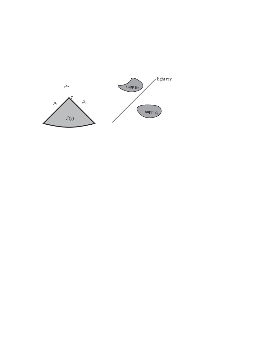
Figure VI.1. Relative position of the point $y$ for the factorization of the TOP and of the $\operatorname{supp}g_{1}$ for the factorization of $\mathbb{S}$.

Given a set of points $x_{1},\ldots,x_{n}$ we ask whether there is a partition of it such that at least one of the points lies in the causal past of all the others. Evidently, this is possible, only if the points do not all coincide ($x_{1}=x_{2}=\ldots=x_{n}$). Therefore, if at least one pair of points does not coincide, it is possible to construct the $n$-th order TOP. The renormalization problem, in this scheme, manifests itself as the problem of extending the $n$-th order TOP to the diagonal. The TOP are, however, operator-valued distributions with values in an algebra $\mathcal{W}$ (to be defined later). Instead of searching for an extension of OVDs, one reduces the problem to the extension of c-number-valued distributions with the help of the Wick expansion.

Theorem VI.2 (Wick expansion)

The product of Wick polynomials can be expressed as a sum of Wick polynomials. Without loss of generality we have

$$:\psi^{*}(x_{1})\psi(x_{1}):\ldots:\psi^{*}(x_{n})\psi(x_{n}):\cdot:\psi^{*}(y)\psi(y):=\sum_{m=0}^{n+1}d_{m}(x_{1},\ldots,x_{n},y)\ :\psi^{*}\psi^{(m)}:,$$

where $:\psi^{*}\psi^{(m)}:$ is the Wick product of $m$-th order which contains $m$ field operators and $m$ adjoint field operators. The $d_{m}$ denote number-valued distributions.

Focusing attention on the TOP of the order $n$, $T_{n}$, we may factorize it to become a product of lower order TOP’s and, after Wick expansion we obtain the $n$-th order TOP in the form

$$T_{n}(x_{1},\ldots,x_{n})=T[\mathcal{L}(x_{1})\ldots\mathcal{L}(x_{n})]=\sum_{m=0}^{n+1}t^{0}_{m}(x_{1},\ldots,x_{n})\ :\psi^{*}\psi^{(m)}:,$$

where the distributions $t^{0}_{m}(x_{1}\ldots x_{m})$ are known for all points with the exception of the diagonal $x_{1}=\ldots=x_{m}$. We need to extend it to the diagonal, because the evolution operator $\mathbb{S}(g)$ smears the time-ordered product $T_{n}(x_{1},\ldots,x_{n})$ with the same test function $g(x)$ in every variable, and hence the diagonal belongs to the support of the product of the test functions.

If relative coordinates are employed, for instance $x_{i}^{a}=x_{0}^{a}+\xi_{i}^{a}$, then the diagonal coincides with the origin of the $(\mathbb{R}^{4})^{\times n}$ space, where $\xi^{i}=0$. There is an elegant way to extend distributions singular at the origin to that point, if only the distributions are homogeneous. If we require that the scaling of the distribution must be preserved by the extension, then the following possibilities arise:

• the extension to the diagonal is unique (this is usually the case in the so-called tree Feynman diagrams) and may be obtained, for instance, by multiplying the Wick expansions for different configurations of points with an appropriate step (Heaviside) distributions;

• the extension to the diagonal is not unique (which is the case in the loop-containing Feynman diagrams) and is characterized by a finite number of free parameters, which correspond to the renormalization constants.

The truncated evolution operator $\mathbb{S}$, constructed with the help of the time-ordered products of order not greater than $n$ and smeared with test functions $g(x)$ which specify the interaction region, describes the quantum electrodynamics in finite-order perturbation theory. The results obtained in this way correspond [Sch96] to those obtained in the other formulations of the perturbation theory (which in our opinion have a less transparent structure).

VI.2. Algebra of Wick polynomials

Let from now on $\hbox{$O\iota^{\prime}\acute{}\hskip 3.0pt$}(\mathcal{O})$ denote the CAR algebra of the free Dirac field. The region $\mathcal{O}$ is an open bounded region in spacetime which additionally is geodesically convex (a double-cone). In order to incorporate the interacting field we shall investigate algebras larger than $\hbox{$O\iota^{\prime}\acute{}\hskip 3.0pt$}(\mathcal{O})$. In particular, we will define the algebra $\mathcal{W}(\mathcal{O})$ which also contains the Wick polynomials of the free fields. Before we define $\mathcal{W}(\mathcal{O})$ consider the Wick square of the free Dirac field.

Example.

The Wick squares are defined by the point-splitting limit:

$$:\psi^{*}\psi:(x) =\lim_{y\rightarrow x}\left[\psi^{*}(x)\psi(y)-\tilde{d}(x,y)\right],$$ (VI.2a)

$$:\psi\psi^{*}:(x) =\lim_{y\rightarrow x}\left[\psi(x)\psi^{*}(y)-d(x,y)\right],$$ (VI.2b)

with appropriate distributions $d(x,y),\tilde{d}(x,y)$. The smeared Wick square is a functional of one test function:

$$:\psi^{*}\psi:(f)=\int d^{4}x\ d^{4}y\left[\psi^{*}(x)\psi(y)-d(x,y)\right]\ \delta(x-y)f(x).$$

The above formula looks as if we have smeared the ordinary operator-valued distribution

$$\psi^{*}(x)\psi(y)-d(x,y),$$

(which when smeared with two test functions becomes an operator belonging to $O\iota^{\prime}\acute{}\hskip 3.0pt$ and is well-defined for all $d(x,y)$) with the distribution $\delta(x-y)f(x)$. The result is an OVD in the algebra of Wick polynomials $\mathcal{W}$ irrespective of $d(x,y)$. However, in order to find a representation of this algebra it will be necessary to restrict the class of allowed $d(x,y)$.

Definition VI.3 (Wick products of $n$-th order)

The Wick product of $n$-th order is a regularization of the product of $n$ field operators and $n$ adjoint filed operators (grouped in pairs). It is defined inductively in terms of Wick products of order $n-1$ and lower. Let $d(x,y)$ and $\tilde{d}(x,y)$ denote the two distributions which have the same wave front set:

$$WF^{\prime}(d)=\{(x,\xi,y,\xi):x\sim y,\xi_{0}\geq 0\}.$$

The $n$-th order product is given by

$$:\psi^{*}(x_{1})\psi(y_{1})\dots\psi^{*}(x_{n})\psi(y_{n}):\ \doteq\psi^{*}(x_{1})\psi(y_{1})\dots\psi^{*}(x_{n})\psi(y_{n})-\\ -\sum_{k,l}A(x_{k},y_{l})\ :\psi^{*}(x_{1})\psi(y_{1})\dots\psi^{*}(x_{l})\widetilde{\psi(y_{l})}\dots\widetilde{\psi^{*}(x_{k})}\psi(y_{k})\dots\psi^{*}(x_{n})\psi(y_{n}):-\\ \ (contraction\ of\ two\ pairs\ \psi\psi^{*}):(product\ of\ remaining\ operators):-\\ -\ {\sum_{k=3}^{n}(contractions\ of\ k\ pairs)\ :product\ of\ (n-k)\ pairs:},$$

where $A(x_{k},y_{l})$ denotes either $d(x_{k},y_{l})$ in case $l<k$ or $\tilde{d}(x_{k},y_{l})$ in the other case. The tilde denotes the operators which do not appear (have been contracted). The Wick product of an equal number of field operators and their adjoints in arbitrary order is defined similarly, the only difference is that in front of each contraction there is a factor $(-1)^{j}$, where $j$ is the number of permutations necessary in order to bring the contracted operators together.

Remark.

The definition of Wick products makes use of only two distributions $d,\tilde{d}$. It is assumed that they regularize the two-point functions of Hadamard states, namely, the distributions

$$\omega (\psi_{A}(x)\psi^{*}_{B}(z))-d_{AB}(x,z),$$

$$\omega (\psi^{*}_{B}(z)\psi_{A}(x))-\tilde{d}_{BA}(z,x)$$

are assumed to be smooth for every Hadamard state $\omega$. The pointwise product of $d$ and $\tilde{d}$ is well-defined as a distribution, due to the properties of their wave front sets. The multiplication enlarges the wave front set; for instance, $d(x,y)\tilde{d}(x,y)$ has the wave front set

$$WF^{\prime}(d\tilde{d})=\{(x,\xi_{1},y,\xi_{2}):\xi_{i}\in J^{+}\}.$$

This set is stable under further multiplications with distributions having the Hadamard form of singularity [BF00].

Lemma VI.4

Let $\mathcal{F}$ be the Hilbert space constructed upon a Hadamard state $\omega$. The Wick products defined above, even upon multiplication with $\delta(x_{i}-y_{j})$, are operator-valued distributions on $\mathcal{F}$.

Remark.

We do not prove this lemma here, although for second-order Wick products it is not difficult. The generalization to higher order products for the scalar field has been given in [BF00]. In order to use these results here we would need a characterization of the Wick products in terms of derivatives of certain functionals which we do not have at the moment.

In what follows we shall prove a lemma which greatly facilitates the Wick ordering of the time-ordered products.

Lemma VI.5

If the regularizing distributions fulfill the condition

$$d_{AB}(x,y)+\tilde{d}_{BA}(y,x)=S_{AB}(x,y)=\{\psi_{A}(x),\psi^{*}_{B}(y)\},$$

then the Wick products change sign upon commutation of adjacent field operators:

$$:\psi^{*}(x_{1})\psi(y_{1})\ldots\psi^{*}(a)\psi(b)\ldots\psi^{*}(x_{n})\psi(y_{n}):\ =\\ =-:\psi^{*}(x_{1})\psi(y_{1})\ldots\psi(b)\psi^{*}(a)\ldots\psi^{*}(x_{n})\psi(y_{n}):.\$$

Proof.

The proof is standard and can be completed with combinatoric methods. We shall consider the case when the commutation occurs right at the end of the Wick product. The LHS in that case is

$$LHS=\psi^{*}(x_{1})\psi(y_{1})\ldots\psi^{*}(x_{n})\psi(y_{n})\ \psi^{*}(a)\psi(b)+contractions.$$

The RHS is similarly

$$RHS=\psi^{*}(x_{1})\psi(y_{1})\ldots\psi^{*}(x_{n})\psi(y_{n})\ \psi^{*}(a)\psi(b)+\\ -S(b,a)\ \psi^{*}(x_{1})\psi(y_{1})\ldots\psi^{*}(x_{n})\psi(y_{n})+\widetilde{contractions},$$

where ”$contractions$” means all the due terms from the expansion of

$$:\psi^{*}(x_{1})\psi(y_{1})\ldots\psi^{*}(x_{n})\psi(y_{n})\ \psi^{*}(a)\psi(b):.$$

Similarly, ”$\widetilde{contractions}$” means all the due terms from the expansion of

$$-:\psi^{*}(x_{1})\psi(y_{1})\ldots\psi^{*}(x_{n})\psi(y_{n})\ \psi(b)\psi^{*}(a):.$$ (VI.3)

Evidently, the products of field operators are equal on both sides; what remains to be done is to show that the terms with contractions are also equal. Let us take the RHS and consider the two possible cases:

• There is a contraction of $\psi^{*}(a)$ or $\psi(b)$ with the other points. Then in the Wick product there is a minus sign due to the even number of field operators between the contracted quantities. This minus compensates the minus of the whole expansion (VI.3), and what remains after the contraction corresponds precisely to the respective term of the expansion on the LHS.

• The operators $\psi(b)\psi^{*}(a)$ are contracted together. This leads to the term

  $$d(b,a)\ [all\ contractions\ of\ :\psi^{*}(x_{1})\psi(y_{1})\ldots\psi^{*}(x_{n})\psi(y_{n}):],$$

  which is equal to

  $$d(b,a)\ [\psi^{*}(x_{1})\psi(y_{1})\ldots\psi^{*}(x_{n})\psi(y_{n})].$$

  If we combine this with the other summand on the RHS (which involves $S(b,a)$) it yields

  $$-\tilde{d}(a,b)\ [\psi^{*}(x_{1})\psi(y_{1})\ldots\psi^{*}(x_{n})\psi(y_{n})],$$

  which is precisely the sum of contractions on the LHS in the case of $\psi(a)\psi^{*}(b)$ contracted together.

∎

Remark.

As a simplest corollary we note that

$$:\psi(x)\psi^{*}(y):=-:\psi(y)\psi^{*}(x):.$$

Also

$$:\psi^{*}(x)\psi(x)\psi^{*}(y)\psi(y):=:\psi^{*}(y)\psi(y)\psi^{*}(x)\psi(x):.$$

Both the above expressions facilitate greatly the causal Wick expansion of the second order TOP (see section VI.6.2).

With this preparatory definitions we may now define the larger algebra $\mathcal{W}(\mathcal{O})$ which will be large enough to contain the non-linear field quantities, in particular the interacting fields.

Definition VI.6

On the distributional level the algebra $\mathcal{W}(\mathcal{O})$ is the algebra generated by the Wick polynomials of an even number of elements

$$W_{2}(x,y) =\ :\psi^{*}(x)\psi(y):,$$

$$W_{4}(x_{1},x_{2},y_{1},y_{2}) =\ :\psi^{*}(x_{1})\psi(y_{1})\psi^{*}(x_{2})\psi(y_{2}):,$$

$$\vdots\qquad =\qquad\vdots,$$

possibly multiplied with delta-distributions in order to define Wick powers. The elements of the algebra $\mathcal{W}(\mathcal{O})$ are formed, when the resulting quantity is integrated with the test functions of compact support in $\mathcal{O}$:

$$\mathcal{W}(\mathcal{O})\ni W(g_{1},\dots,g_{n})=\int d^{4}x_{1}\dots d^{4}x_{n}\ g_{1}(x_{1})\cdot\dots\cdot g_{n}(x_{n})\ W(x_{1},\dots,x_{n}),$$

where for brevity we have omitted the remaining arguments $y_{1},\dots,y_{n}$ which should also be smeared with the test functions.

Remark.

In applications the expectation values of the elements of $\mathcal{W}$ will be studied. The expectation values of the Wick products $W_{n}(x_{1},\ldots,x_{n})$ will become harmless smooth functions, but their distributional coefficients $c_{n}$ will require investigation (see the expression (VI.9) for a concrete example).

VI.3. Locality in causal perturbation theory

In this section we will introduce a new condition of locality for quantum field theory on external backgrounds. This new locality requirement will be stronger than the notion of locality usually employed in quantum field theory without external field backgrounds. In what follows we will define this new notion and explain why it is necessary to incorporate it in the construction of the quantum electrodynamics. We shall put less emphasis on the mathematical rigor of the definition of locality in favor of a clarification of its physical meaning.

The standard notion of locality in quantum field theory means that the observables in spatially separated regions should be commensurate. More precisely, if we focus on the algebras of observables $\hbox{$O\iota^{\prime}\acute{}\hskip 3.0pt$}(\mathcal{O})$ parameterized by spacetime regions, we have the following

Definition VI.7 (Quantum field theoretical locality)

The net of algebras $\hbox{$O\iota^{\prime}\acute{}\hskip 3.0pt$}(\mathcal{O})$ is local, if each $A\in\hbox{$O\iota^{\prime}\acute{}\hskip 3.0pt$}(\mathcal{O})$ commutes with all the elements of the algebras of the regions spatially related to $\mathcal{O}$, that is

$$[A,B]=0\qquad\forall\ A\in\hbox{$O\iota^{\prime}\acute{}\hskip 3.0pt$}(\mathcal{O}),\ B\in\hbox{$O\iota^{\prime}\acute{}\hskip 3.0pt$}(\mathcal{O}^{\prime}),\ \mathcal{O}\ /\backslash\tilde{\mathcal{O}}.$$

The notation $\mathcal{O}\ /\backslash\tilde{\mathcal{O}}$ means, that the regions $\mathcal{O}$ and $\tilde{\mathcal{O}}$ cannot be connected by a causal curve.

As far as the standard notion of locality is concerned, there is the following, simple

Observation VI.8

The Wick squares defined above are local in the field-theoretical sense (def. VI.7), and this property is independent of the choice of the regularizing distribution $d(x,y)$.

Proof.

We investigate the commutator

$$[:\psi^{*}_{A}\psi_{B}:(x),:\psi^{*}_{C}\psi_{D}:(y)],$$

where the points $x$ and $y$ are spacelike related. If we undo the point-splitting limit and order the expression appropriately we obtain

$$[.,.]=S_{BC}(x^{\prime},y)\psi^{*}_{A}(x)\psi(y^{\prime})-S_{DA}(y^{\prime},x)\psi^{*}_{C}(y)\psi_{B}(x^{\prime}),$$

which is independent of $d(x,y)$ and vanishes, due to the properties of the anti-commutator distribution. ∎

VI.3.1. Local quantum field theory on external field backgrounds

At this point we may ask, whether it follows form observation VI.8 that any choice of the regularizing distribution $d(x,y)$ leads to a local theory. If the definition VI.7 is all we ask for, then indeed the net of Wick polynomial algebras $\mathcal{W}(\mathcal{O})$ are local. However, there is a stronger locality requirement that is in the spirit of general relativity. This requirement, called the Local Position Invariance (LPI), lies at the foundation of the theory of relativity; it is instructive to recall its definition and the way it has been tested experimentally. Local position invariance states that:

The outcome of any non-gravitational experiment is independent of where and when in the universe it is performed. The fundamental constants of non-gravitational physics should be constants in space and time.

In experiments the LPI is measured with the help of the following procedure (see figure VI.2): two precise frequency standards (the atomic clocks) are employed. They are synchronized with a light signal. They follow their wordlines and continuously send the light signals which carry the information about their states. Those signals are compared at a single event. The result is scrutinized against general relativistic predictions, namely, one calculates the geometric lengths of both wordlines. If the time lapse the atomic clocks have measured is proportional to the length of their wordlines, then indeed the non-gravitational experiments (here the quantum optical experiments) are independent of the position in the universe.

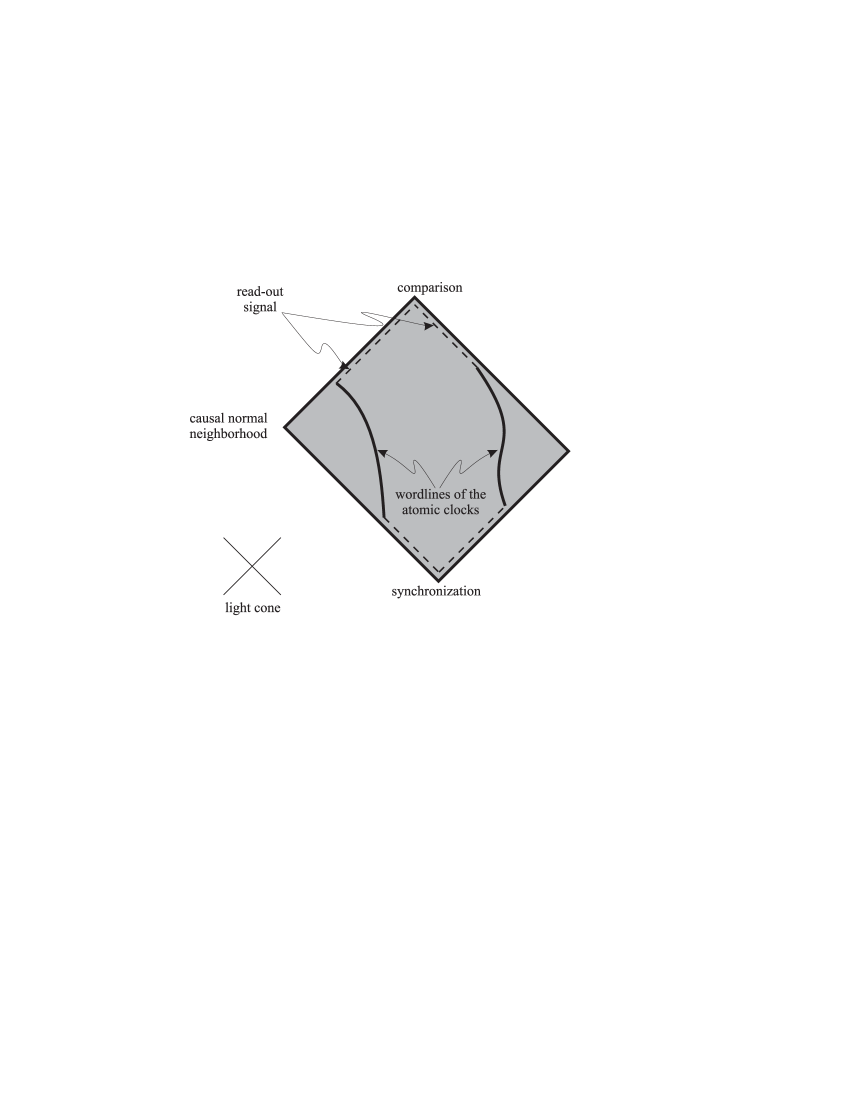
Figure VI.2. GPS-like test of local position invariance. The experimental result is allowed to depend only on the gravitational field in the causal normal neighborhood containing the whole measurement apparatus (together with the final signal read-out).

Let us view the experiment described above from a different perspective and ask what does the result of the measurement (of the comparison) depend on? Clearly, if the LPI is fulfilled, then the result depends only on the gravitational field in the region of spacetime which contains the wordlines of the two detectors and all the geodesics which join them (the clocks must be synchronized and their state must be compared). Therefore, the LPI which at the moment is supported by strong experimental evidence [Wi01] implies that the results of quantum optical experiments can only depend on the external field in the causal neighborhood containing the entire measurement setup.

We now turn back to the definition of local quantum field theory. Recall that the quantum field theory consists of three main ingredients:

• an algebra of observables $\mathcal{W}(\mathcal{O})$, on which

• the time evolution acts as a group of automorphisms;

• the states are functionals on $\mathcal{W}(\mathcal{O})$; they describe the expectation values of the observables.

In this paper we have adapted the following way to incorporate the LPI into quantum field theory.

Definition VI.9 (Strong locality)

The quantum field theory is local in a strong sense (LPI) if:

• The bi-distribution employed in the definition of the Wick square ($d(x,y)$) and of all Wick polynomials (see Wick expansion, theorem VI.2), is a functional of the external field (and its derivatives). In particular

  $$d(x,y)=d[A,\partial A,\partial^{2}A,\ldots].$$

• The distributional coefficients of the Wick powers, $c_{n}(x_{1},\ldots,x_{n})$, are also functionals of the external field.

• All the above distributions depend functionally only on the external field in the causal normal neighborhood which contains all of their arguments. Specifically, if $g(x)$ denotes an arbitrary test function of compact support, then the functional derivatives of $\langle d,g\otimes g\rangle$ and $\langle c_{n},g^{\otimes n}\rangle$, with respect to the external field $A(z)$, must necessarily vanish:

  $$\frac{\delta\,\langle d,g\otimes g\rangle}{\delta A(z)} =0, \frac{\delta\,\langle c_{n},g^{\otimes n}\rangle}{\delta A(z)} =0,$$

  if the point $z$ does not belong to the smallest causal normal neighborhood containing the support of $g$ (see figure VI.3).

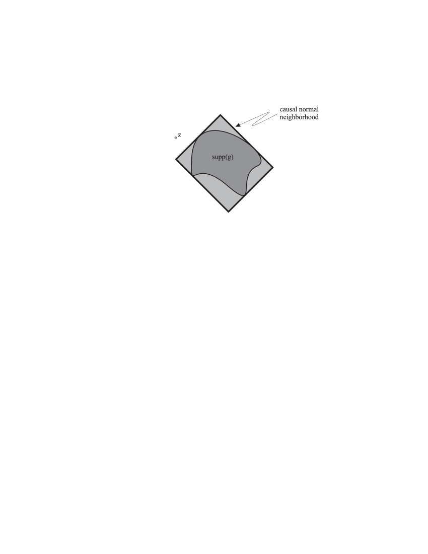
Figure VI.3. Smallest causal neighborhood containing the support of the test function $g$. The point $z$ lies outside of it.

Remark.

As a consequence of the strong locality requirement we may compare two quantum field theories on different external fields, say $A$ and $\tilde{A}$. If those external fields match in a geodesically convex neighborhood $\mathcal{O}$, the Wick algebras $\mathcal{W}_{A}(\mathcal{O})$ and $\mathcal{W}_{\tilde{A}}(\mathcal{O})$ may be identified (are naturally isomorphic). This leads to the picture of a local quantum field theory as a functor between the categories of all possible external field configurations and the category of unital $C^{*}$-algebras. In this framework it is possible to investigate the change of algebraic elements under the compactly supported variation of the external field (relative Cauchy evolution) [BFV01]. It is important to stress, however, that the notion of locality takes into account only the two first ingredients of a quantum field theory: the observables and their time evolution. There is an intrinsic non-locality in the construction of states of the quantum field (this is discussed in the next section). We should also note the new insight into the LPI of general relativity which is gained from the quantum field theory on external field backgrounds, namely, it is not true that there exist ”non-gravitational experiments” at all. Even the local influence of the external field may lead to the alternation of non-gravitational phenomena such as the atomic dynamics. This together with the non-locality of the two point function of the radiation field, which in the view of the appendix D influences the atomic emission process, is a possible way to try to explain the decrease of the fine structure constant at distant epochs recently observed with the help of very modern methods by J.K.Webb and collaborators [Web02].

VI.4. Non-locality of the two-point functions

In this section we show that the two-point functions $G_{\pm}(x,y)$ contain information about the external field not only in the causal neighborhood of $x$ and $y$, and thus they do not fulfill the strong locality requirement VI.9.

We construct our argument for the massless, hermitian, scalar field, as in that case the argument is transparent and simple. Let the external potential be static and only dependent on one spatial variable, say $x_{3}$, called ”$x$” in the sequel. Investigate the classical scattering, stationary wave functions in order to define the field operator with their help.

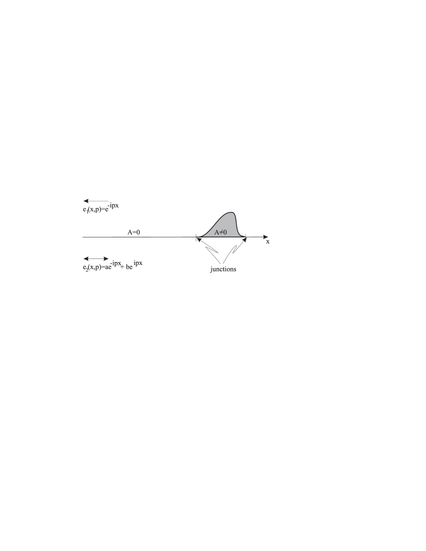
Figure VI.4. Two independent solutions $e_{1}(x)$ and $e_{2}(x)$. The other dimensions $(t,{\mathbf{x}}_{\bot})$ are suppressed.

The $x_{1}$ and $x_{2}$ (called ”${\mathbf{x}}_{\bot}$” for brevity) dependence factorizes:

$$u(t,{\mathbf{x}})=e^{iE(p_{\bot},p)t-i{\mathbf{p}}_{\bot}{\mathbf{x}}_{\bot}}\cdot e(p,x).$$

As there is no external field for small $x$, both independent solutions $e_{1,2}(x,p)$ will be linear combinations of the running waves: outgoing $e^{-ipx}$ and incoming $e^{ipx}$. We may take as the first solution the one for which $e_{1}=e^{-ipx}$ (which is a purely outgoing wave) for small $x$. The second solution, orthogonal to $e_{1}$, will have the form

$$e_{2}=ae^{-ipx}+be^{ipx},$$

where $a\neq 0$, because there is a potential scattering, $b\neq 0$ because it needs to be orthogonal to $w_{1}$. Now the field can be quantized in a standard manner. We introduce the object (later, the field-operator-valued-distribution)

$$\psi(t,x,x_{\bot})=\int_{\mathbb{R}^{2}}d^{2}p_{\bot}\int_{0}^{\infty}\frac{dp}{\sqrt{2E({\mathbf{p}}_{\bot},p)}}\ \cdot\left\{e^{iEt-ip_{\bot}x_{\bot}}[e_{1}(x,p)a_{1}({\mathbf{p}})+e_{2}(x,p)a_{2}({\mathbf{p}})]+H.c.\right\},$$

with the CCR for the $a$’s :

$$[a_{1}({\mathbf{p}}),a^{*}_{1}({\mathbf{k}})] =\delta({\mathbf{p}}-{\mathbf{k}}), [a_{1}({\mathbf{p}}),a^{*}_{2}({\mathbf{k}})] =0,$$

$$[a_{2}({\mathbf{p}}),a^{*}_{2}({\mathbf{k}})] =\delta({\mathbf{p}}-{\mathbf{k}}), [a_{.}({\mathbf{p}}),a_{.}({\mathbf{k}})] =0.$$

Note that we have two sets of creation/annihilation operators, because we have separated the positive and negative values of $p=p_{3}$.

The vacuum representation is defined by requiring

$$a_{.}({\mathbf{p}})\Omega=0.$$

Now the two point function $(\Omega,\psi({\mathbf{x}})\psi({\mathbf{y}})\ \Omega)$ (for equal times) is given by

$$\int_{\mathbb{R}^{2}}d^{2}p_{\bot}\int_{0}^{\infty}\frac{dp}{2E}\ \cdot\left\{e^{-ip_{\bot}(x-y)_{\bot}}[e_{1}(x_{3})\overline{e}_{1}(y_{3})+e_{2}(x_{3})\overline{e}_{2}(y_{3})]\right\}.$$

The square bracket is evaluated to be

$$[\ldots]=(1+|a|^{2})e^{-ip(x-y)}+|b|^{2}e^{ip(x-y)}+a\overline{b}\ e^{ip(x+y)}+\overline{a}b\ e^{-ip(x+y)}.$$

On the other hand in the absence of the external field we have

$$[\ldots]_{Minkowski}=e^{-ip(x-y)}+e^{ip(x-y)}.$$

Both distributions are not equal. $\quad\Box$

We infer from the above example that the two-point function contains non-local information. We cannot implement the strong locality requirement VI.9 by employing objects constructed with the help of the two-point functions.

VI.5. Non-localities of the extensions of local distributions

The construction of interacting field theory, as outlined in section VI.1, requires an extension of the time-ordered products to the coincidence point, where the appropriate $c$-number-valued distributions are singular. In this section, by means of an example, we discuss the difficulties arising in the extension process.

Suppose that the appropriate distribution $t^{0}(x)$ away from the diagonal already fulfills the strong locality requirement. Moreover, suppose that the singularity of the distribution $t^{0}$ is such that its action is well-defined for all test functions that vanish at the origin $x=0$. The following simple method of extension of $t^{0}$ to the origin is generically employed in the usual causal perturbation theory: define the subtraction $\mathfrak{w}$ on the space of test functions

$$(\mathfrak{w}f)(x)=f(x)-w(x)f(0)\quad\forall f\in\mathcal{C}_{0}^{\infty}(\mathbb{R}),$$

where $w(x)$ is an arbitrary $\mathcal{C}_{0}^{\infty}$-function equal to $1$ in the vicinity of $x=0$. The extended distribution (denoted by $t$) is defined by

$$\langle t,f\rangle=\langle t^{0},\mathfrak{w}f\rangle.$$ (VI.4)

Evidently, the extension $t$ coincides with the distribution $t^{0}$, if the test function vanishes at the origin. Moreover, the difference of two different extensions, characterized by $w_{1}$ and $w_{2}$, is given by

$$\langle t_{1}-t_{2},f\rangle=\langle t_{0},w_{2}-w_{1}\rangle f(0),$$

which is a distribution supported only at the origin, and therefore (which is a general property - see [HC66]) can be expressed as a sum of the delta-distribution and its derivatives. If we additionally require the extension to have the same scaling behavior as $t_{0}$, we can say which derivatives of $\delta$ appear. In the case of $t^{0}(x)=1/x$ the result is

$$t_{2}(x)=t_{1}(x)+c\ \delta(x)$$

with an arbitrary constant $c$. For instance, the Cauchy principal value:

$$\langle P\tfrac{1}{x},g\rangle=\lim_{\epsilon\rightarrow 0}\int_{|x|\geq\epsilon}\frac{g(x)}{x}$$

and the $i\epsilon$ prescription

$$t^{0}=\frac{1}{x+i\epsilon}$$ (VI.5)

are precisely two different extensions of the distribution $t^{0}=1/x$ which differ by a $c\cdot\delta(x)$ distribution (with $c=-i\pi$).

Let us consider the difficulties with the strong locality requirement (definition VI.9) which arise in the presence of external fields. Suppose the distribution $t^{0}$ was local in the strong sense and had the same singularity structure as $1/x$. An example of such a distribution is

$$t^{0}(x)=\frac{\int_{0}^{1}A(xs)\ ds}{x}$$

which shares some similarity with the first term of the parametrix of the Klein-Gordon operator on an external background $A(x)$. The extension of this distribution by means of the $\mathfrak{w}$ subtraction is

$$\langle t,f\rangle=\langle t^{0},\mathfrak{w}f\rangle=\int dx\ ds\ \frac{1}{x}A(sx)\ [f(x)-w(x)f(0)].$$ (VI.6)

The conflict with the strong locality principle is now evident. The general extension depends not only on the external field in the support of $f(x)$, which would be the manifestation of strong locality, but also on the external field in the region of support of $w(x)$, which spoils the locality (if $\operatorname{supp}w\subset\!\!\!\!\!/\operatorname{supp}f$).

A further investigation is therefore needed in order to make the renormalization method of Epstein and Glaser [DM75, BF00] strongly local.

VI.6. Local causal perturbation theory in the lowest orders

In this section we shall construct local Wick and time-ordered products of first and second order. They are the building blocks of the evolution operator $\mathbb{S}$ (when smeared out with test functions), and it is essential to investigate them carefully, as any alternation of their form can potentially lead to the modification of measurable quantities. The second order time-ordered product already describes a number of important phenomena.

We begin this section with some considerations of the lowest two orders of Wick and time-ordered products of the standard approach to the external field quantum electrodynamics. They are not local in the strong sense, as has been explained before. We present them nonetheless, because this discussion will be of help in the construction of the local Wick and time-ordered products, and because it may help the reader to recognize the more familiar objects and realize where the necessary modification will be done, in order to make these objects local.

In quantum electrodynamics the first order time-ordered product is given by the interaction term $\mathcal{L}_{I}$:

$$T_{1}(x)=\mathcal{L}_{I}(x)=ie:\overline{\psi}_{A}(x)\mathchoice{\gamma_{\kern 0.0pt\hbox{$\scriptstyle\mu\hbox{}\hbox{}$}}^{\hbox{$\scriptstyle{}$}\kern 0.0pt\hbox{$\kern 0.0pt\scriptstyle\hbox{}AB$}}}{\gamma_{\kern 0.0pt\hbox{$\scriptstyle\mu\hbox{}\hbox{}$}}^{\hbox{$\scriptstyle{}$}\kern 0.0pt\hbox{$\kern 0.0pt\scriptstyle\hbox{}AB$}}}{\gamma_{\kern 0.0pt\hbox{$\scriptscriptstyle\mu\hbox{}\hbox{}$}}^{\hbox{$\scriptscriptstyle{}$}\kern 0.0pt\hbox{$\kern 0.0pt\scriptscriptstyle\hbox{}AB$}}}{\gamma_{\kern 0.0pt\hbox{$\scriptscriptstyle\mu\hbox{}\hbox{}$}}^{\hbox{$\scriptscriptstyle{}$}\kern 0.0pt\hbox{$\kern 0.0pt\scriptscriptstyle\hbox{}AB$}}}\psi_{B}(x):\ \mathcal{A}^{\mu}(x).$$

The second order time-ordered product satisfies the causality relation

$$T_{2}(x,y)=T_{1}(x)T_{1}(y),$$

if only $y\in/J^{+}(x)$. Thus, for $x\neq y$ the fermionic part of the second order TOP can be brought into the form:

$$T_{2}(x,y)=\sum_{n=0}^{2}\ t_{n}(x,y)\ :\psi^{*}\psi^{(n)}:$$

with the help of the Wick expansion VI.2. The Wick products on the RHS are independent of the relative position of the points, but the distributions $t_{n}(x,y)$ are at first defined only for non-coinciding points.

VI.6.1. Usual Wick product

Now we will recall some facts about the Wick product of two Dirac field operators. Let there be a fixed representation of the free CAR algebra with the base state described by a vector $\Omega$ in the Hilbert space. We introduce the commonly employed abbreviations

$$i\mathchoice{G_{\kern 0.0pt\hbox{$\scriptstyle\hbox{}AB$}}^{\hbox{$\scriptstyle{}$}\kern 0.0pt\hbox{$\kern 0.0pt\scriptstyle+\hbox{}\hbox{}$}}}{G_{\kern 0.0pt\hbox{$\scriptstyle\hbox{}AB$}}^{\hbox{$\scriptstyle{}$}\kern 0.0pt\hbox{$\kern 0.0pt\scriptstyle+\hbox{}\hbox{}$}}}{G_{\kern 0.0pt\hbox{$\scriptscriptstyle\hbox{}AB$}}^{\hbox{$\scriptscriptstyle{}$}\kern 0.0pt\hbox{$\kern 0.0pt\scriptscriptstyle+\hbox{}\hbox{}$}}}{G_{\kern 0.0pt\hbox{$\scriptscriptstyle\hbox{}AB$}}^{\hbox{$\scriptscriptstyle{}$}\kern 0.0pt\hbox{$\kern 0.0pt\scriptscriptstyle+\hbox{}\hbox{}$}}}(x,y) \doteq(\Omega,\psi_{A}(x)\overline{\psi}_{B}(y)\Omega),$$

$$i\mathchoice{G_{\kern 0.0pt\hbox{$\scriptstyle\hbox{}AB$}}^{\hbox{$\scriptstyle{}$}\kern 0.0pt\hbox{$\kern 0.0pt\scriptstyle-\hbox{}\hbox{}$}}}{G_{\kern 0.0pt\hbox{$\scriptstyle\hbox{}AB$}}^{\hbox{$\scriptstyle{}$}\kern 0.0pt\hbox{$\kern 0.0pt\scriptstyle-\hbox{}\hbox{}$}}}{G_{\kern 0.0pt\hbox{$\scriptscriptstyle\hbox{}AB$}}^{\hbox{$\scriptscriptstyle{}$}\kern 0.0pt\hbox{$\kern 0.0pt\scriptscriptstyle-\hbox{}\hbox{}$}}}{G_{\kern 0.0pt\hbox{$\scriptscriptstyle\hbox{}AB$}}^{\hbox{$\scriptscriptstyle{}$}\kern 0.0pt\hbox{$\kern 0.0pt\scriptscriptstyle-\hbox{}\hbox{}$}}}(x,y) \doteq(\Omega,\overline{\psi}_{A}(x)\psi_{B}(y)\Omega).$$

The (non-local) Wick products are defined by

$$:\psi_{A}(x)\overline{\psi}_{B}(y): \doteq\psi_{A}(x)\overline{\psi}_{B}(y)-iG^{+}_{AB}(x,y),$$ (VI.7a)

$$:\overline{\psi}_{A}(x)\psi_{B}(y): \doteq\overline{\psi}_{A}(x)\psi_{B}(y)-iG^{-}_{AB}(x,y).$$ (VI.7b)

Note that the Wick products are not linear and the definition (VI.7b) cannot be derived from (VI.7a) with the help of the anti-commutation relations. In the case of absent external field the distributions $G^{\pm}(x,y)$ are well-known:

$$i\mathchoice{G_{\kern 0.0pt\hbox{$\scriptstyle\hbox{}AB$}}^{\hbox{$\scriptstyle{}$}\kern 0.0pt\hbox{$\kern 0.0pt\scriptstyle+\hbox{}\hbox{}$}}}{G_{\kern 0.0pt\hbox{$\scriptstyle\hbox{}AB$}}^{\hbox{$\scriptstyle{}$}\kern 0.0pt\hbox{$\kern 0.0pt\scriptstyle+\hbox{}\hbox{}$}}}{G_{\kern 0.0pt\hbox{$\scriptscriptstyle\hbox{}AB$}}^{\hbox{$\scriptscriptstyle{}$}\kern 0.0pt\hbox{$\kern 0.0pt\scriptscriptstyle+\hbox{}\hbox{}$}}}{G_{\kern 0.0pt\hbox{$\scriptscriptstyle\hbox{}AB$}}^{\hbox{$\scriptscriptstyle{}$}\kern 0.0pt\hbox{$\kern 0.0pt\scriptscriptstyle+\hbox{}\hbox{}$}}}(x,y) =\frac{1}{(2\pi)^{3}}\int\frac{d^{3}p}{2p_{0}}(p/+m)e^{-ip(x-y)},$$

$$i\mathchoice{G_{\kern 0.0pt\hbox{$\scriptstyle\hbox{}AB$}}^{\hbox{$\scriptstyle{}$}\kern 0.0pt\hbox{$\kern 0.0pt\scriptstyle-\hbox{}\hbox{}$}}}{G_{\kern 0.0pt\hbox{$\scriptstyle\hbox{}AB$}}^{\hbox{$\scriptstyle{}$}\kern 0.0pt\hbox{$\kern 0.0pt\scriptstyle-\hbox{}\hbox{}$}}}{G_{\kern 0.0pt\hbox{$\scriptscriptstyle\hbox{}AB$}}^{\hbox{$\scriptscriptstyle{}$}\kern 0.0pt\hbox{$\kern 0.0pt\scriptscriptstyle-\hbox{}\hbox{}$}}}{G_{\kern 0.0pt\hbox{$\scriptscriptstyle\hbox{}AB$}}^{\hbox{$\scriptscriptstyle{}$}\kern 0.0pt\hbox{$\kern 0.0pt\scriptscriptstyle-\hbox{}\hbox{}$}}}(x,y) =\frac{1}{(2\pi)^{3}}\int\frac{d^{3}p}{2p_{0}}(p/-m)e^{-ip(x-y)}.$$

We may write

$$iG^{+}_{AB}(x,y)=(i\partial/_{x}+m)_{AB}\cdot\Delta^{+}(x,y),$$

$$iG^{-}_{AB}(x,y)=(i\partial/_{x}-m)_{BA}\cdot\Delta^{+}(x,y),$$

where $\Delta^{+}(x,y)$ denotes the massive ($m$), scalar, vacuum two-point function. It is important to stress that both $G^{+}$ and $G^{-}$ are derivatives of the same distribution. Consequently, the wave front set of $\Delta^{+}$ contains the wave front sets of $G^{\pm}$.

The anti-commutator distribution $G_{AB}(x,y)$ can be expressed in terms of $G^{\pm}$:

$$iG_{AB}(x,y)=\{\psi_{A}(x),\overline{\psi}_{B}(y)\}=(\Omega,\{\psi_{A}(x),\overline{\psi}_{B}(y)\}\ \Omega)=iG^{+}_{AB}(x,y)+iG^{-}_{BA}(y,x),$$ (VI.8)

which assures the validity of the lemma on the (anti)commutation of Wick products (lemma VI.5). We also note that

$$iG_{AB}(x,y)=\{\psi_{A}(x),\psi_{C}^{*}(y)\}\ \mathchoice{\gamma_{\kern 0.0pt\hbox{$\scriptstyle\hbox{}B$}}^{\hbox{$\scriptstyle{}$}\kern 0.0pt\hbox{$\kern 0.0pt\scriptstyle 0C\hbox{}$}}}{\gamma_{\kern 0.0pt\hbox{$\scriptstyle\hbox{}B$}}^{\hbox{$\scriptstyle{}$}\kern 0.0pt\hbox{$\kern 0.0pt\scriptstyle 0C\hbox{}$}}}{\gamma_{\kern 0.0pt\hbox{$\scriptscriptstyle\hbox{}B$}}^{\hbox{$\scriptscriptstyle{}$}\kern 0.0pt\hbox{$\kern 0.0pt\scriptscriptstyle 0C\hbox{}$}}}{\gamma_{\kern 0.0pt\hbox{$\scriptscriptstyle\hbox{}B$}}^{\hbox{$\scriptscriptstyle{}$}\kern 0.0pt\hbox{$\kern 0.0pt\scriptscriptstyle 0C\hbox{}$}}}=S_{AC}(x,y)\mathchoice{\gamma_{\kern 0.0pt\hbox{$\scriptstyle\hbox{}B$}}^{\hbox{$\scriptstyle{}$}\kern 0.0pt\hbox{$\kern 0.0pt\scriptstyle 0C\hbox{}$}}}{\gamma_{\kern 0.0pt\hbox{$\scriptstyle\hbox{}B$}}^{\hbox{$\scriptstyle{}$}\kern 0.0pt\hbox{$\kern 0.0pt\scriptstyle 0C\hbox{}$}}}{\gamma_{\kern 0.0pt\hbox{$\scriptscriptstyle\hbox{}B$}}^{\hbox{$\scriptscriptstyle{}$}\kern 0.0pt\hbox{$\kern 0.0pt\scriptscriptstyle 0C\hbox{}$}}}{\gamma_{\kern 0.0pt\hbox{$\scriptscriptstyle\hbox{}B$}}^{\hbox{$\scriptscriptstyle{}$}\kern 0.0pt\hbox{$\kern 0.0pt\scriptscriptstyle 0C\hbox{}$}}},$$

and we find, in accordance with C.4, the equal-time anti-commutation relation

$$iG_{AB}({\mathbf{x}},{\mathbf{y}})=\gamma^{0}_{AB}\ \delta({\mathbf{x}}-{\mathbf{y}}).$$

The Wick product of the free electromagnetic fields is defined by

$$:\mathcal{A}_{\mu}(x)\mathcal{A}_{\nu}(y):\ =\mathcal{A}_{\mu}(x)\mathcal{A}_{\nu}(y)-\eta_{\mu\nu}\Delta^{+}_{0}(x,y),$$

where $\Delta^{+}_{0}(x,y)$ denotes the massless, scalar field two-point function (III.7).

VI.6.2. Second-order time-ordered product

Turning now towards the second order TOP, $T_{2}(x,y)$, in the case $y\in/J^{+}(x)$, we will use the causal Wick expansion to order of the expression

$$T_{2}(x,y)=(ie)^{2}:\overline{\psi}_{A}(x)\gamma^{\mu AB}\psi_{B}(x)::\overline{\psi}_{C}(y)\gamma^{\nu CD}\psi_{D}(y):\ \mathcal{A}_{\mu}(x)\mathcal{A}_{\nu}(y).$$

As $T_{1}$ already involved a limiting procedure (in the case of the Dirac field operators), in order to Wick-expand $T_{2}$ we will step back this limit and consider

$$T_{2}(x,y)=(ie)^{2}\left[:\overline{\psi}_{A}(x)\psi_{B}(x^{\prime})::\overline{\psi}_{C}(y)\psi_{D}(y^{\prime}):\right]\gamma^{\mu AB}\ \gamma^{\nu CD}\ \mathcal{A}_{\mu}(x)\mathcal{A}_{\nu}(y),$$

where only the square-bracket term requires further attention. It is seen to be equal to

$$[\ldots]=\overline{\psi}_{A}(x)\psi_{B}(x^{\prime})\overline{\psi}_{C}(y)\psi_{D}(y^{\prime})-iG^{-}_{AB}(x,x^{\prime}):\overline{\psi}_{C}(y)\psi(y^{\prime}):-\\ -iG^{-}_{CD}(y,y^{\prime}):\overline{\psi}_{A}(x)\psi_{B}(x^{\prime}):+G^{-}_{AB}(x,x^{\prime})G^{-}_{CD}(y,y^{\prime}).$$

The first term should now be Wick-expanded. This leads to the expression in which the limit $x^{\prime}\rightarrow x$ and $y^{\prime}\rightarrow y$ can be taken. One obtains:

$$T_{2}(x,y)=-e^{2}\left[:\overline{\psi}_{A}(x)\psi_{B}(x)\overline{\psi}_{C}(y)\psi_{D}(y):+iG^{-}_{AD}(x,y):\psi_{B}(x)\overline{\psi}_{C}(y):+\right.\\ \left.+iG^{+}_{BC}(x,y):\overline{\psi}_{A}(x)\psi_{D}(y):-G^{-}_{AD}(x,y)G^{+}_{BC}(x,y)\right]\gamma^{\mu AB}\gamma^{\nu CD}\\ \left[:\mathcal{A}_{\mu}(x)\mathcal{A}_{\nu}(y):+\eta_{\mu\nu}\Delta^{+}_{0}(x,y)\right].$$ (VI.9)

The pointwise product of $G^{-}_{AD}(x,y)G^{+}_{BC}(x,y)$ is well-defined, and its wave front set is not greater than that of $\Delta^{+}(x,y)^{2}$.

In the other case, when $x\in/J^{+}(y)$, there is

$$T_{2}(x,y)=T_{1}(y)T_{1}(x),$$

and the similar Wick expansion can be performed. We only have to exchange $x$ with $y$ (and also $A$ with $C$, $B$ with $D$ and $\mu$ with $\nu$). The causal Wick expansion requires ,however, to order $T_{1}(y)T_{1}(x)$ in such a way that the Wick products in $T_{2}(x,y)$ are the same as in (VI.9). In order to do that we employ the (anti)commutation lemma VI.5. We arrive at

$$T_{1}(y)T_{1}(x)=-e^{2}\left[:\overline{\psi}_{A}(x)\psi_{B}(x)\overline{\psi}_{C}(y)\psi_{D}(y):-iG^{+}_{DA}(y,x):\psi_{B}(x)\overline{\psi}_{C}(y):+\right.\\ \left.-iG^{-}_{CB}(y,x):\overline{\psi}_{A}(x)\psi_{D}(y):-G^{+}_{DA}(y,x)G^{-}_{CB}(y,x)\right]\gamma^{\mu AB}\gamma^{\nu CD}\\ \left[:\mathcal{A}_{\mu}(x)\mathcal{A}_{\nu}(y):+\eta_{\mu\nu}\Delta^{+}_{0}(y,x)\right].$$ (VI.10)

A comparison of the above expression with (VI.9) is presented in the table 1.

$y\in/J^{+}(x)$	$x\in/J^{+}(y)$
$G^{-}_{AD}(x,y)$	$-G^{+}_{DA}(y,x)$
$G^{+}_{BC}(x,y)$	$-G^{-}_{CB}(y,x)$
$G^{-}_{AD}(x,y)G^{+}_{BC}(x,y)$	$G^{+}_{DA}(y,x)G^{-}_{CB}(y,x)$
$\Delta^{+}_{0}(x,y)$	$\Delta^{+}_{0}(y,x)$

Table VI.1. Correspondence of factors of Wick products with different relative position of the points $x$ and $y$.

What remains to be done in order to define the $T_{2}(x,y)$ for all its arguments is to extend the distributional factors of Wick products to the diagonal $x=y$. Thus, in accordance with the general procedure (see section VI.1), the definition of $T_{2}$ for all $x,y$ reduces to the problem of the extension of number-valued distributions, which are known for $x\neq y$, to the diagonal $x=y$. Some of the distributions appearing in $T_{2}(x,y)$ can be extended to the diagonal uniquely; the other, however, have a family of extensions parameterized by what is known as the renormalization constants.

VI.6.3. Local definition of the Wick product

The Wick products defined with the help of the $G^{\pm}$ are not local in the strong sense. We shall repair this deficiency in what follows.

In order to make the Wick square an operator-valued distribution it is necessary only to remedy the short-distance singularities of the product of the field operators. We proceed therefore and give a local expression for the Wick product, the uniqueness of which will be analyzed in a separate section (see section VI.7.2). The leading short-distance singularities of the expectation value of the product of the Dirac-field operators in some Hadamard state are all contained in the (local) Hadamard parametrix $H_{AB}(x,y)$ constructed in chapter IV. We therefore define

$$:\psi_{A}(x)\overline{\psi}_{B}(y):\doteq\psi_{A}(x)\overline{\psi}_{B}(y)-H_{AB}(x,y)$$

and, similarly,

$$:\overline{\psi}_{A}(x)\psi_{B}(y):\doteq\overline{\psi}_{A}(x)\psi_{B}(y)-\tilde{H}_{AB}(x,y),$$

where the Hadamard parametrix $\tilde{H}$ must be separately derived with the methods of chapter IV for the case of the adjoint Dirac operator acting on the variable $x$:

$$\tilde{H}_{AB}(x,y)\ \overleftarrow{D^{a}_{x}}\mathchoice{\,{}_{\kern 0.0pt\hbox{$\scriptstyle\hbox{}C$}}^{\hbox{$\scriptstyle{}$}\kern 0.0pt\hbox{$\kern 0.0pt\scriptstyle A\hbox{}$}}}{\,{}_{\kern 0.0pt\hbox{$\scriptstyle\hbox{}C$}}^{\hbox{$\scriptstyle{}$}\kern 0.0pt\hbox{$\kern 0.0pt\scriptstyle A\hbox{}$}}}{\,{}_{\kern 0.0pt\hbox{$\scriptscriptstyle\hbox{}C$}}^{\hbox{$\scriptscriptstyle{}$}\kern 0.0pt\hbox{$\kern 0.0pt\scriptscriptstyle A\hbox{}$}}}{\,{}_{\kern 0.0pt\hbox{$\scriptscriptstyle\hbox{}C$}}^{\hbox{$\scriptscriptstyle{}$}\kern 0.0pt\hbox{$\kern 0.0pt\scriptscriptstyle A\hbox{}$}}}=0,$$

with

$$\overleftarrow{D^{a}_{x}}\mathchoice{\,{}_{\kern 0.0pt\hbox{$\scriptstyle\hbox{}C$}}^{\hbox{$\scriptstyle{}$}\kern 0.0pt\hbox{$\kern 0.0pt\scriptstyle A\hbox{}$}}}{\,{}_{\kern 0.0pt\hbox{$\scriptstyle\hbox{}C$}}^{\hbox{$\scriptstyle{}$}\kern 0.0pt\hbox{$\kern 0.0pt\scriptstyle A\hbox{}$}}}{\,{}_{\kern 0.0pt\hbox{$\scriptscriptstyle\hbox{}C$}}^{\hbox{$\scriptscriptstyle{}$}\kern 0.0pt\hbox{$\kern 0.0pt\scriptscriptstyle A\hbox{}$}}}{\,{}_{\kern 0.0pt\hbox{$\scriptscriptstyle\hbox{}C$}}^{\hbox{$\scriptscriptstyle{}$}\kern 0.0pt\hbox{$\kern 0.0pt\scriptscriptstyle A\hbox{}$}}}=(-i\overleftarrow{\partial/}-m+eA/)\mathchoice{\,{}_{\kern 0.0pt\hbox{$\scriptstyle\hbox{}C$}}^{\hbox{$\scriptstyle{}$}\kern 0.0pt\hbox{$\kern 0.0pt\scriptstyle A\hbox{}$}}}{\,{}_{\kern 0.0pt\hbox{$\scriptstyle\hbox{}C$}}^{\hbox{$\scriptstyle{}$}\kern 0.0pt\hbox{$\kern 0.0pt\scriptstyle A\hbox{}$}}}{\,{}_{\kern 0.0pt\hbox{$\scriptscriptstyle\hbox{}C$}}^{\hbox{$\scriptscriptstyle{}$}\kern 0.0pt\hbox{$\kern 0.0pt\scriptscriptstyle A\hbox{}$}}}{\,{}_{\kern 0.0pt\hbox{$\scriptscriptstyle\hbox{}C$}}^{\hbox{$\scriptscriptstyle{}$}\kern 0.0pt\hbox{$\kern 0.0pt\scriptscriptstyle A\hbox{}$}}}.$$

We therefore establish the following substitution rule for the Wick products:

$$H_{AB}(x,y) \leftrightarrow iG^{+}_{AB}(x,y),$$

$$\tilde{H}_{AB}(x,y) \leftrightarrow iG^{-}_{AB}(x,y).$$

The definition of the Wick product with the help of the Hadamard parametrix encounters, however, two obstacles: on the one hand the full series defining $H_{AB}(x,y)$ is convergent, only if the external fields are analytic functions (which is a narrow case), on the other hand the full $H_{AB}(x,y)$ is of no practical use, as it is unknown how to sum up the Hadamard series.

If the coincidence limit $y\rightarrow x$ is of interest (that is if only powers of the field are of interest), then an observation of V.Moretti, [Mor01], is helpful, namely:

Observation VI.10

The Wick product $:\psi_{A}(x)\overline{\psi}_{B}(x):$ can be defined with finitely many terms of the Hadamard expansion (in this case all what is needed are $u,v_{0}\mbox{ and }v_{1}$). The so-defined OVD fulfills the wave equation (the Dirac equation) in its variable modulo a constant:

$$\lim_{x\rightarrow y}D_{x}:\psi_{A}(x)\overline{\psi}_{B}(y):=3\,\mathcal{D}_{x}v_{0}(x)|_{x=y}$$

(with abbreviations of chapter IV, note that $D_{x}$ and $\mathcal{D}_{x}$ are different).

Proof.

As the field operator $\psi_{A}(x)$ fulfills the field equation by definition, what remains to be done is the inspection of

$$\lim_{x\rightarrow y}D_{x}H^{N}(x,y),$$

where $H^{N}(x,y)$ is the Hadamard parametrix without the smooth term $w(x,y)$ and cut at $v_{N}$. Not surprisingly the calculation which preceded the derivation of the transport equations (IV.5d) will be helpful, for

$$\lim_{x\rightarrow y}D_{x}H^{N}(x,y)=\lim_{x\rightarrow y}\mathcal{D}_{x}\phi^{N}(x,y).$$

By inspection, we conclude that $\mathcal{D}_{x}\phi^{N}(x,y)$ consists of terms proportional to $1/\Gamma^{2},\ 1/\Gamma$, $\ln\Gamma$ as well as $\Gamma^{n}$ and $\Gamma^{n}\ln\Gamma$. All three first, singular terms will vanish as long as $N\geq 1$ due to the transport equations fulfilled by $u,v_{0}$ and $v_{1}$. The coefficients of the powers of $\Gamma$ will have no effect in the limit $x\rightarrow y$. What will remain, however, is the coefficient of $\Gamma^{0}$ which defined the transport equation for $w_{1}(x,y)$ set to zero in our case. One finds

$$\lim_{x\rightarrow y}\mathcal{D}_{x}\phi^{N}(x,y)=\lim_{x\rightarrow y}\mathcal{D}_{x}\phi^{1}(x,y)=-v_{1}(12+B^{a}\partial_{a}\Gamma)-2\partial^{a}\Gamma\partial_{a}v_{1}=-4v_{1}+\mathcal{D}_{x}v_{0},$$

as a consequence of (IV.5c). Now, from the recursion relation, we have

$$v_{1}(x,y)=-\tilde{u}(x,y)\int_{0}^{1}\tau d\tau\,\left.\frac{\mathcal{D}_{w}v_{0}(w,y)}{\tilde{u}(w,y)}\right|_{w=y+\tau(x-y)},$$

in the limit $x\rightarrow y$

$$v_{1}(y,y)=-\frac{1}{2}\mathcal{D}_{x}v_{0}(x,y)|_{\,x=y}.$$

∎

VI.7. Local definition of the current operator; back-reaction effects

In this section we formulate the problem of the back reaction of the quantum fields on the background arena. Let us recall the field equations of the theory developed in this paper (cf. chapter I):

$$\left[i\gamma^{a}\partial^{x}_{a}+eA_{a}^{class}(x)-m\right]\psi(x) =-e\mathcal{A}_{a}(x)\psi(x),$$ (VI.11a)

$$\partial^{b}_{x}F^{\mathcal{A}}_{ab}(x) =4\pi\ \overline{\psi}(x)\gamma_{a}\psi(x),$$ (VI.11b)

$$\partial^{b}_{x}F_{ab}^{class}(x) =4\pi J_{a}(x),$$ (VI.11c)

where $A^{class}\equiv A$ is the classical electromagnetic field which is the background field, $\mathcal{A}$ is the quantum electromagnetic field, $\psi$ is the quantum Dirac field and $J$ is the external classical current which is the source of the $A$-field. The interaction of the quantum fields (the RHS of the first two equations) is treated in a perturbative way.

The main assumption of the theory is that the external current $J$ is not influenced by the state of the quantized radiation field $\mathcal{A}$. We propose the following way to assess this influence: if the current produced by the quantized Dirac field is comparable (locally) to $J$, then the external field approximation is not reliable anymore.

Suppose that we focus on the current density $J^{0}(x)$ and the current-density operator $\rho(x)$ (to be defined later). There are three issues arising, if we want to make the above criterion more precise. Firstly, for a given state $|F\rangle$ of the Dirac field it is insufficient to compare the expectation value $(F,\rho(x)F)$ to $J^{0}(x)$. The current-density operator is not positive, and therefore one should also investigate higher momenta of it, for instance $(F,\rho(x)\rho(x)F)$.

The second issue is that we have only the statistical interpretation of quantum theory, and thus we do not really know what happens in a single experiment. This is related to the problem of measurement. If the results of quantum theory such as $\langle\rho^{2}(x)\rangle$ do correspond only to the average over many experimental realizations, why then should in a single experiment the back-reaction effect be governed by such an average? Let us put this question in a physical context: Imagine a weakly localized electron which, upon an interaction with a measurement device, for instance a CCD camera, produces a sharply localized, strong effect - a macroscopically visible trace. The CCD camera is composed of various charges and could have been regarded, for instance, as the source of the classical current density $J^{0}$. Therefore, even arbitrarily low current densities can produce intensive back-reaction effects. This shows that the phenomenological criterion we have put forward in order to judge the possible back-reaction effects can fail for some sources of the external current $J$.

In quantum field theory there is an additional difficulty. The current-density operator has to be defined as a coincidence limit of a difference between the two-point function of the state of the quantum field and a certain regularizing bi-distribution. This bi-distribution in the no-external-field case is taken simply to be the vacuum expectation value of the appropriate (bi-local) current-density operator. However, as we have discussed in the chapter II there is no privileged state of the Dirac field on external field backgrounds. How should the current-operator be defined? It is precisely the strong locality criterion (definition VI.9) that allows for a definition of the absolute current density. In other words, the strong locality criterion allows us to separate the (state-independent) singularity of the two-point function from the state-dependent information which may cause the back reaction.

What follows in this section deals with the definition of the current operator $j^{\mu}(x)$. We shall define it for the free Dirac field by the point-splitting procedure. The quantum version of $j^{\mu}(x)$ should correspond to the classical current

$$j_{class}^{\mu}=e\ \overline{\psi}(x)\gamma^{\mu}\psi(x).$$

It should also posses the following properties:

• In the time-independent case, the integration of $j^{0}(x)$ over a Cauchy surface,

  $$Q=\int d^{3}x\ j^{0}({\mathbf{x}}),$$

  should correspond to the total charge operator $Q=e(N^{+}-N^{-})$, where $N^{\pm}$ are electron-/positron-number operators.

• The current operator should be conserved

  $$\partial_{\mu}j^{\mu}(x)=0.$$

We recall that the classical current is conserved as a consequence of the Dirac equation and its adjoint, namely the (co)-spinors $\overline{\psi}(x)$, $\psi(x)$ fulfill

$$[i\partial/+eA/(x)-m]\psi(x) =0,$$

$$\overline{\psi}(x)\ [-i\overleftarrow{\partial/}+eA/-m] =0,$$

from which conservation of the current follows immediately.

As a first candidate for the current-density operator we investigate

$$j^{\mu}(x)=:\overline{\psi}(x)\gamma^{\mu}\psi(x):_{\omega}=\lim_{y\rightarrow x}[\overline{\psi}(y)\gamma^{\mu}\psi(x)-iG^{-}_{AB}(y,x)\gamma^{\mu AB}],$$ (VI.12)

where $iG^{-}_{AB}(y,x)=(\Omega,\overline{\psi}(y)\psi(x)\ \Omega)$. The above operator is not local in that it depends on the external field in the regions other than the infinitesimal neighborhood of $x$; nonetheless we shall consider its features. Let us look at the total charge. We find

$$\int d^{3}x\ j^{0}(x)=\int d^{3}x\ \int d\mu_{p}\ d\mu_{k}\ \left[u^{\dagger}(x,{\mathbf{p}})u(x,{\mathbf{k}})a^{*}({\mathbf{p}})a({\mathbf{k}})-v^{\dagger}(x,{\mathbf{p}})v(x,{\mathbf{k}})b^{*}({\mathbf{k}})b({\mathbf{p}})\right]+\\ +\int d^{3}x\ \int d\mu_{p}\ d\mu_{k}\ \left[u^{\dagger}(x,{\mathbf{p}})v(x,{\mathbf{k}})a^{*}({\mathbf{p}})b^{*}({\mathbf{k}})+v^{\dagger}(x,{\mathbf{p}})u(x,{\mathbf{k}})b({\mathbf{k}})a({\mathbf{p}})\right].$$

Now, due to

$$(u({\mathbf{k}}),u({\mathbf{p}})) =\delta({\mathbf{k}}-{\mathbf{p}}), (v({\mathbf{k}}),v({\mathbf{p}})) =\delta({\mathbf{k}}-{\mathbf{p}}),$$

$$(u({\mathbf{k}}),v({\mathbf{p}})) =0,$$

we obtain

$$\int d^{3}x\ j^{0}(x)=\int d\mu_{p}\left[a^{*}({\mathbf{p}})a({\mathbf{p}})-b^{*}({\mathbf{p}})b({\mathbf{p}})\right],$$

which is just the total current $Q=e(N^{+}-N^{-})$.

VI.7.1. Charge conservation, local definition of the current density

The non-locality of (VI.12) was not the only shortcoming of this expression. It is easy to see that the so-defined current density is not conserved. Indeed, as the differentiation is performed before the coincidence limit $y\rightarrow x$ is taken, the $\overline{\psi}$-terms are not differentiated and, consequently, the current is not conserved.

With regard to the point-splitting procedure of defining $j^{\mu}$ there are therefore two issues:

• The conservation of the current density.

• The appropriate behavior of the coincidence limit.

Various procedures have been devised in the literature to remedy both of the above problems. The main theme of those procedures is:

• to remedy the non-conservation by means of the symmetrization of $j^{\mu}(x,y)$ w.r.t. its variables;

• to assure the finiteness of the $x\rightarrow y$ limit by a subtraction of a certain local bi-distribution.

A current density which fulfills all our requirements and which is constructed as indicated above is:

$$j^{\mu}(x)=\lim_{y\rightarrow x}[\overline{\psi}(y)\gamma^{\mu}\psi(x)-\mbox{H}_{AB}(y,x)\gamma^{\mu AB}+\overline{\psi}(x)\gamma^{\mu}\psi(y)-\mbox{H}_{AB}(x,y)\gamma^{\mu AB}].$$ (VI.13)

VI.7.2. Uniqueness of the current operator

The uniqueness of the current operator is connected with the uniqueness of the Wick square of the field operators. Suppose that we alter the definition of the Wick product by terms of lower order in the field operators:

$$:\overline{\psi}\psi:=\overline{\psi}\psi-\tilde{d}(x,y)\gamma^{0}+c(x)\psi+d(x)\psi^{*}+f(x,y)\mathbf{1}.$$

If we require the current to be selfadjoint and to fulfill the standard locality requirement VI.7, then we must have $c=0=d$. In order to further restrict the remaining ambiguity we use the locality requirement, namely, the function $f(x,y)$ can depend functionally only on the external field in the smallest causal neighborhood of $x$ and $y$. In the point splitting limit this should become a functional of the external field at the point $x$. Such functionals are known to be functions of the external field $A(x)$ and its derivatives $\partial_{x}A(x)$. If we further require these functions to be analytic in the external field and the mass $m$ of the Dirac field, we can expand $f(x,x)$ as a power series in $A$, $\partial^{n}A$ for all $n$, and in the mass $m$. Furthermore, the Wick product must have a dimension of $1/cm^{3}$ and both the external field $A$ and the mass $m$ have dimension $1/cm$. Due to this and the Lorentz condition $\partial A=0$, we obtain the result

Lemma VI.11

The local current-density operator is unique up four arbitrary numbers $a_{1}\ldots a_{4}$. Any two local definitions differ at most by

$$\Delta:j^{\mu}:(x)=a_{1}\ A^{\nu}\partial_{\nu}A^{\mu}+a_{2}\ m^{2}A^{\mu}+a_{3}\ A_{\nu}A^{\nu}A^{\mu}+a_{4}\ \Box A^{\mu}$$

VI.8. Scaling transformations for local observables

In this section the (re)scaled non-linear observables will be investigated. The purpose of the scaling is to approach the short scale-limit of the theory.

VI.8.1. Scaling transformation in the scalar case

In the following we shall investigate the behavior of local observables costructed out of the scalar massive fields under scaling.

In analogy to the extraction of the long-range part of the electromagnetic field introduced by Gervais and Zwanziger [GZ80],

$$A_{a}^{long}(x)=\lim_{\lambda\rightarrow\infty}\ \lambda A_{a}(\lambda x),$$

we shall associate with a (classical) scalar massive field $\varphi(x)$ a field $\tilde{\varphi}(x)$ rescaled by $\lambda$:

$$\tilde{\varphi}(x)=\lambda\varphi(\lambda x).$$

We define the scaling transformation for classical quantities:

Definition VI.12 (classical rescaling)

A scaling transformation $\sigma$ is a prescription to obtain various quantities at a different scale $\lambda$, where $\lambda\rightarrow 0$ corresponds to the short-distance limit. In order to investigate the rescaled theory we

• rescale all quantities, that is

  $$\sigma:f(x,y,\ldots)\rightarrow f(\lambda x,\lambda y,\ldots);$$

• interpret the result in terms of the rescaled field

  $$\tilde{\varphi}(x)=\lambda\varphi(\lambda x).$$

As an example, let us find the field equation fulfilled by $\tilde{\varphi}$. We rescale

$$0=\sigma\left[(\Box_{x}+m^{2})\varphi(x)\right]=(\lambda^{-2}\Box_{x}+m^{2})\varphi(\lambda x)=\lambda^{-3}(\Box_{x}+\lambda^{2}m^{2})\tilde{\varphi}(x)=0,$$

and therefore $\tilde{\varphi}(x)$ is a massive scalar field with the smaller mass $\lambda m$.

Now we shall define the scaling of the (massive, hermitean, scalar) quantum field

Definition VI.13 (quantum rescaling)

The scaling transformation is a prescription which transforms operator-valued distributions constructed with the help of the (linear) quantum field $\varphi(x)$ on the GNS Hilbert space of the state $\omega$ into an operator-valued distributions of the scaled quantum field $\tilde{\varphi}(x)$ on the GNS Hilbert space of the scaled state $\tilde{\omega}$. The two-point functions of the respective states are related by:

$$\tilde{\omega}(x,y)=\lambda^{2}\omega(\lambda x,\lambda y).$$

Remark.

The scaling transformation relates the quantities of one quantum dynamical system to the other. The dynamical laws in both systems are different, as the field operators $\varphi(x)$ and $\tilde{\varphi}(x)$ fulfill different field equations. Both systems (on a single Cauchy surface) are representations of the same CCR algebra:

$$[\varphi({\mathbf{x}}),\varphi({\mathbf{y}})] =\delta({\mathbf{x}}-{\mathbf{y}}), [\tilde{\varphi}({\mathbf{x}}),\tilde{\varphi}({\mathbf{y}})] =\delta({\mathbf{x}}-{\mathbf{y}}).$$

Even on this single surface, however, the states $\omega$ and $\tilde{\omega}$ are not even locally equivalent; as we shall see, their short distance singularity structure is different.

As an example let us investigate the scaling of the Wick product which is given by

$$:\varphi(x)\varphi(y):\doteq\varphi(x)\varphi(y)-H(x,y),$$

where $H(x,y)$ is a certain bi-distribution, for instance

$$H(x,y)=\frac{1}{\Gamma}+m^{2}\ln(\Gamma m^{2}).$$

Let us now perform the scaling $\sigma$ on the Wick product. We have

$$\sigma_{\lambda}[:\varphi(x)\varphi(y):]=\frac{1}{\lambda^{2}}[\lambda^{2}\varphi(\lambda x)\varphi(\lambda y)-\lambda^{2}H(\lambda x,\lambda y)]=\frac{1}{\lambda^{2}}[\tilde{\varphi}(x)\tilde{\varphi}(y)-H_{\lambda}(x,y)],$$

where we have denoted the rescaled regularizing bi-distribution by $H_{\lambda}$:

$$H_{\lambda}(x,y)=\lambda^{2}H(\lambda x,\lambda y)=\frac{1}{\Gamma}+(\lambda m)^{2}\ln\left[\Gamma(\lambda m)^{2}\right].$$

The singularity structure of $H_{\lambda}$ clearly differs form $H$ (as long as the field is massive). It is also evident that in the short distance limit $\lambda\rightarrow 0$ the less singular term in $H_{\lambda}$ will disappear,

$$\lim_{\lambda\rightarrow 0}H_{\lambda}(x,y)=\frac{1}{\Gamma}=\Delta_{0}^{+}(x,y),$$

where $\Delta_{0}^{+}(x,y)$ is the vacuum, massless two-point function.

VI.9. Scaling transformation for the Dirac field in external potentials

The action for the classical Dirac field on a background external potential $A_{a}(x)$ is given by

$$S=\int\mbox{d${}^{4}$x }\left\{[i\hbar\ \overline{\psi}\gamma^{a}\partial_{a}\psi-mc\ \overline{\psi}\psi]-[\overline{\psi}\gamma^{a}\psi\ \frac{e}{c}A_{a}]\right\}$$

Here the action is dimensionless and the Dirac field $\psi(x)$ has a dimension of cm^-3/2. Analogously to the scalar case, the scaling is performed by a substitution $x\rightarrow\lambda x$. Here, however, the rescaled field (classical and quantum) is defined via

$$\tilde{\psi}(x)=\lambda^{3/2}\psi(\lambda x).$$

Again the scaling transformation transforms operator-valued distributions on the GNS Hilbert space $\mathcal{F}$ into the operator-valued distributions on the GNS Hilbert space $\tilde{\mathcal{F}}$ constructed with the help of

$$\tilde{\omega}(x,y)=\lambda^{3}\omega(\lambda x,\lambda y).$$

Remark.

Similarly to the scalar-field case, we note that on a fixed Cauchy surface the OVD $\psi(x)$ and $\tilde{\psi}(x)$ fulfill the same anti-commutation relations. However,

• they obey a different dynamical law, and

• the state $\tilde{\omega}$ is not locally equivalent to $\omega$.

It is interesting to note that if we introduce the rescaled external field $\tilde{A}$ and the rescaled mass $\tilde{m}$,

$$\tilde{m} =\lambda m, \tilde{A}_{a}(x) =\lambda A_{a}(\lambda x),$$

then for all operator-valued distributions $F[x,y,\ldots\psi(x),A,m]$ there is

$$\sigma\left\{F[x,y,\ldots,\psi(x),A,m]\right\}=F[x,y,\ldots,\tilde{\psi}(x),\tilde{A},\tilde{m}].$$

An investigation of the Wick product

$$:\psi_{A}(x)\overline{\psi}_{B}(y):=\psi_{A}(x)\overline{\psi}_{B}(y)-H_{AB}(x,y),$$

with $H_{AB}$ chosen to be a parametrix (with certain $w_{0}(x,y)$) dependent on $m$ and the external field $A_{a}(x)$ as explained in chapter VI.6, reveals

$$\sigma_{\lambda}[:\psi_{A}(x)\overline{\psi}_{B}(y):]=\frac{1}{\lambda^{3}}[:\psi_{A}(x)\overline{\psi}_{B}(y):-H_{\lambda\ AB}(x,y)]$$

with

$$H_{\lambda\ AB}(x,y)=\lambda^{3}H_{AB}(\lambda x,\lambda y),$$

being the scaled Hadamard parametrix. In what follows $H_{\lambda\ AB}$ will be investigated in greater detail.

VI.9.1. Scaling of the Hadamard parametrix for the Dirac field

In chapter IV we have found the Hadamard parametrix $H_{AB}(x,z)$ of the Dirac field. It was given by

$$H_{AB}(x,z)=(i\gamma^{a}\partial_{a}+e\gamma^{a}A_{a}(x)+m\mathchoice{)_{\kern 0.0pt\hbox{$\scriptstyle A\hbox{}$}}^{\hbox{$\scriptstyle{}$}\kern 0.0pt\hbox{$\kern 0.0pt\scriptstyle\hbox{}C$}}}{)_{\kern 0.0pt\hbox{$\scriptstyle A\hbox{}$}}^{\hbox{$\scriptstyle{}$}\kern 0.0pt\hbox{$\kern 0.0pt\scriptstyle\hbox{}C$}}}{)_{\kern 0.0pt\hbox{$\scriptscriptstyle A\hbox{}$}}^{\hbox{$\scriptscriptstyle{}$}\kern 0.0pt\hbox{$\kern 0.0pt\scriptscriptstyle\hbox{}C$}}}{)_{\kern 0.0pt\hbox{$\scriptscriptstyle A\hbox{}$}}^{\hbox{$\scriptscriptstyle{}$}\kern 0.0pt\hbox{$\kern 0.0pt\scriptscriptstyle\hbox{}C$}}}\phi_{CB}(x,z),$$

where $\phi_{CB}(x,z)$ is the Hadamard parametrix of the operator

$$\mathcal{D}=[\Box-2ieA^{a}(x)\partial_{a}+m^{2}+e^{2}A^{2}(x)]-\frac{e}{2}\mathchoice{\sigma_{\kern 0.0pt\hbox{$\scriptstyle\hbox{}\hbox{}\hbox{}B$}}^{\hbox{$\scriptstyle{}$}\kern 0.0pt\hbox{$\kern 0.0pt\scriptstyle abA\hbox{}$}}}{\sigma_{\kern 0.0pt\hbox{$\scriptstyle\hbox{}\hbox{}\hbox{}B$}}^{\hbox{$\scriptstyle{}$}\kern 0.0pt\hbox{$\kern 0.0pt\scriptstyle abA\hbox{}$}}}{\sigma_{\kern 0.0pt\hbox{$\scriptscriptstyle\hbox{}\hbox{}\hbox{}B$}}^{\hbox{$\scriptscriptstyle{}$}\kern 0.0pt\hbox{$\kern 0.0pt\scriptscriptstyle abA\hbox{}$}}}{\sigma_{\kern 0.0pt\hbox{$\scriptscriptstyle\hbox{}\hbox{}\hbox{}B$}}^{\hbox{$\scriptscriptstyle{}$}\kern 0.0pt\hbox{$\kern 0.0pt\scriptscriptstyle abA\hbox{}$}}}F_{ab}(x),$$

which was determined with the help of the progressing wave expansion:

$$\phi_{CB}(x,z)=\frac{u_{CB}(x,z)}{\Gamma}+v_{0CB}(x,z)\ln\Gamma+\sum_{1}^{\infty}v_{nCB}(x,z)\Gamma^{n}\ln\Gamma+\sum_{1}^{\infty}w_{nCB}(x,z)\Gamma^{n}$$

where the spinor indices have been restored in order to emphasize the bi-spinorial character of the smooth coefficients $u,v_{n},w_{n}$.

Remark.

The term $\ln\Gamma$ cannot stand as it is, because $\Gamma=(x-z)^{2}$ has a dimension. This dimension can be cancelled with the only length scale available in the theory - the Compton wavelength of the electron. Therefore, everywhere $\ln\Gamma$ should be understood as $\ln(m^{2}\Gamma)$. It is another matter that a different scale (if present) would give a parametrix differing from the above by a smooth function.

Because the parametrix (or certain parts of it ) have been used to define nonlinear quantities, it is important to investigate the scaling properties of the diagonal ($x=z$) values of the smooth coefficients under the transformation $\sigma$. We find the following

Lemma VI.14

The diagonal values $v_{n}(z,z),w_{n}(z,z)$ of the coefficients of the Hadamard parametrix scale under the transformation $\sigma_{\lambda}$ as:

$$\sigma[v_{n}(z)] =\frac{1}{\lambda^{2(n+1)}}\ \tilde{v}_{n}(z),$$

$$\sigma[w_{n}(z)] =\frac{1}{\lambda^{2(n+1)}}\ \tilde{w}_{n}(z),$$

where $n=0,1,\ldots$ for the $v$’s and $n=1,2,\ldots$ for the $w$’s. The $\tilde{v}$ and $\tilde{w}$ denote $v$ and $w$ with $A,m$ replaced by $\tilde{A},\tilde{m}$. The coefficient of the highest singularity $u(z,z)=1$ by assumption for all $\lambda$.

Proof.

Before considering the case of arbitrary $n$, let us first illustrate the reasoning in case of $n=0$ and $n=1$. Everywhere we consider $z$ as a fixed point of reference so that all the differential operators are being taken with respect to the variables other than $z$. We use the abbreviation

$$u(x,z)=\exp\left[ie\chi(x,z)\right]=\exp\left[ie(x-z)^{a}\int_{0}^{1}A_{a}(y)|_{y=z+\tau(x-z)}\ d\tau\right].$$

One easily verifies that in the limit $x\rightarrow z$ there is

$$(\partial_{a}\chi) =A_{a}(z),$$

$$\Box\chi =0,$$

with the last equation being an indirect consequence of the Lorentz gauge of the external field.

The coefficient $v_{0}$ is found from

$$v_{0}(x,z)=-\frac{u}{4}\int_{0}^{1}\frac{\mathcal{D}_{y}u}{u}|_{y_{0}=z+\tau_{0}(x-z)}\ d\tau_{0}.$$

Clearly, in the limit of interest the distributions under the integral become $\tau_{0}$-independent and can be pulled out of the integral, which then assumes the value $1$. Therefore,

$$v_{0}(z,z)=-\frac{1}{4}\mathcal{D}_{y}u(y,z)|_{y=z}.$$

Now the differentiation of $u(y,z)$ results in terms of the sort $\Box_{x}\chi(x,z)$, $A^{a}(x)\partial_{a}\chi(x,z)$, $[m^{2}+e^{2}A^{2}(x)]\cdot\chi(x,z)$, as e.g. explained in and above the formula (IV.16). The scaling means a replacement of $(x,z)$ by $(\lambda x,\lambda z)$. We shall also make use of the rescaled mass and the external field

$$\tilde{m}=\lambda m\qquad\tilde{A}_{a}(x)=\lambda A_{a}(\lambda x).$$

By the explicit formulas for $\chi(x,z)$ and all its derivatives, it is evident that every term of $\mathcal{D}u$ transforms under $\sigma_{\lambda}$ homogeneously with degree $-2$. Therefore, we have

$$\sigma_{\lambda}[v_{0}(z,z)]=\frac{1}{\lambda^{2}}\tilde{v}_{0}(z,z),$$

where $\tilde{v}_{0}$ contains the rescaled $\tilde{A}$ and $\tilde{m}$.

Let us consider then the next coefficient, $v_{1}(x,z)$, which is the prototype of a general situation. According to the formulas of the chapter IV we have:

$$v_{1}(x,z)=\frac{1}{16}u(x,z)\int_{0}^{1}\tau_{1}\ d\tau_{1}\ u^{-1}(y_{1},z)\mathcal{D}_{y_{1}}\left[u(y_{1},z)\int_{0}^{1}u^{-1}(y_{0},z)\mathcal{D}_{y_{0}}u(y_{0},z)\ d\tau_{0}\right],$$

where $y_{1}=z+\tau_{1}(x-z)$ and $y_{0}=z+\tau_{0}(y_{1}-z)$. Now the differential operator $\mathcal{D}_{y_{1}}$ either acts on $u(y_{1},z)$ in front of the integral or can be pulled under the integral, where (as all the expressions there depend only on $y_{0}$) a chain rule has to be invoked which e.g. transforms $\partial_{y_{1}}$ into $\partial_{y_{0}}\cdot\tau_{0}$. In the first case there will be derivatives of $\chi(y_{1},z)$ appearing in front of the $\tau_{0}$-integral, and in the second the derivatives of $\chi(y_{0},z)$ and of $A_{a}(y_{0})$ or $c(y_{0})$. In the limit $x\rightarrow z$ all those factors will become $\tau_{0}$- and $\tau_{1}$-independent (which also assures that they will be functions of the external field at $z$ - and thus - local expressions) and can be pulled out of all the $\tau$-integrals. All the derivatives of $\chi$ are easily seen to have the homogeneous scaling, namely,

$$\sigma_{\lambda}[\partial^{\prime}_{a_{1}}\ldots\partial^{\prime}_{a_{n}}\chi(y,z^{\prime})|_{y=z^{\prime}}=\frac{1}{\lambda^{n}}\chi(z,z).$$

As each differential operator $\mathcal{D}$ contains two such differentiations (or a factor with identical scaling), it follows in particular that

$$\sigma_{\lambda}[v^{\prime}_{1}(z^{\prime},z^{\prime})]=\frac{1}{\lambda^{4}}v_{1}(z,z),$$

and in general

$$\sigma_{\lambda}[v^{\prime}_{n}(z^{\prime},z^{\prime})] =\frac{1}{\lambda^{2(n+1)}}v_{n}(z,z),$$

$$\sigma_{\lambda}[w^{\prime}_{n}(z^{\prime},z^{\prime})] =\frac{1}{\lambda^{2(n+1)}}w_{n}(z,z).$$

The general expressions follow from the recursion relations of chapter IV. ∎

Chapter VII Physical applications

The considerable modification and generalization of existing quantum electrodynamics in strong external fields described in the previous chapters raises two important issues. The first is whether the framework presented in this thesis is concrete enough to describe physical situations. One may ask how to apply the general construction of states of chapter II together with the local causal perturbation theory of chapter VI. The other issue is whether our improvements lead to predictions which differ from the conventional ones. In this chapter we will address the first issue while the second must be deferred to future investigations.

The local causal quantum electrodynamics constructs the local $\mathbb{S}$-matrix which describes the evolution of observables. This $\mathbb{S}$-matrix in each order of perturbation is composed of local Wick and time-ordered products, defined in previous chapters. When smeared out with a test function $g(x)$, all these elements become operators belonging to the algebra $\mathcal{W}$. In order to be able to investigate the physical properties of matter and radiation it is necessary to specify the representation of this algebra and identify in some way the states on this algebra with physical situations. In a concrete representation the non-linear quantities will become operators on a Hilbert space.

The non-linear observables were constructed in such a way that the GNS representation based upon a state $\omega$ of the free field algebra $O\iota^{\prime}\acute{}\hskip 3.0pt$ can be extended to the enlarged algebra $\mathcal{W}$. This extension is possible only, if the two-point function of the state $\omega$ is of Hadamard form (chapter V).

The ”base state” $\omega$ carries with itself the concept of excitations. If $\omega$ is prescribed by a projection operator $P_{+}$, the states of the form $\psi(f_{-})\Omega$, $\psi^{*}(f_{+})\Omega$ with $f_{\pm}=P_{\pm}f\ni\mathcal{H}$ describe excitations which would be conventionally called particles. It is the aim of interacting quantum electrodynamics to investigate the evolution of such excitations.

The identification of mathematical objects with physical reality always has its limits; they are particularly exposed in the interacting theory. Suppose, for instance, that the external field is static. Then the excitations can describe particles in bound states (if such states are allowed by the external field). But what are these states? The quantum electrodynamic interaction changes the dynamics of the Dirac field, and what was stationary in the free theory is not stationary any more in the interacting theory. We would like to know the energy of the excited state 2P of an electron in a hydrogen atom. We describe this state by $\psi^{*}(f_{2P})\Omega$, where $f_{2P}$ is the wave function of the 2P state calculated with the help of the Dirac equation. However, because this state is not stationary, we will never be sure what physical situation it corresponds to or how to produce such a state in experiment.

With this remark in mind we begin to address the first of the issues named at the beginning; in what follows we shall show, how the theory developed in this thesis is applied to describe the simplest non-trivial physical effects.

VII.1. Electrodynamics in the presence of a static background

Static backgrounds are important, mainly because they provide a sufficiently well-characterized and isolated regime for a study of the effects of the QED developed in this thesis. Not only the fully ionized heavy elements (see [Stö98]) but also fine atomic/ionic traps (see [Deh90] and many others) allow for a study of the electrodynamic effects with great precision. In many of these experiments a single electron probes the external field effects. Perhaps for those experimental reasons the conventional literature on the external field QED has focused on static external fields [MPS98, Sha02].

VII.1.1. Vacuum representation, static background

The construction of the vacuum representation in the case of static external backgrounds has been treated in chapter II.3. Here we review it from a more heuristic point of view and restore the appropriate spinor indices.

The free-field operator in the static external fields ”at a point $x$” is an operator-valued distribution which can be decomposed according to:

$$\psi^{A}(x) =\int d^{3}p\ \left\{u^{A}_{s}({\mathbf{x}},{\mathbf{p}})\ e^{-iE^{+}({\mathbf{p}})t}\ a^{s}({\mathbf{p}})+v^{A}_{s}({\mathbf{x}},{\mathbf{p}})\ e^{-iE^{-}(p)t}\ b^{*s}({\mathbf{p}})\right\}+$$

$$+\sum_{n=0}^{N}u_{n}^{A}({\mathbf{x}})\ e^{-iE(n)t}\ a_{n}.$$

Here we have separated the bound states from the scattering states. The $u({\mathbf{x}},{\mathbf{p}})$, $v({\mathbf{x}},{\mathbf{p}})$ denote the positive/negative-frequency scattering states (the index ${\mathbf{p}}$ is continuous). The $u_{n}({\mathbf{x}})$ denote the spinorial wave functions of the bound states, which we have assumed to have positive energies (for simplicity); there may exist an infinite number of them ($N\rightarrow\infty$). The symbols $E^{\pm}({\mathbf{p}})$ denote the energies (the eigenvalues of the time-independent Hamilton operator) of the positive/negative-frequency scattering solutions, respectively. The creaton/annihilation operators obey the standard CAR relations. The vacuum $\Omega$ is the state annihilated by all of the annihilation operators:

$$a({\mathbf{p}})\Omega =0, a_{n}\Omega =0,$$

$$b({\mathbf{p}})\Omega =0.$$

VII.1.2. First-order processes, creation of the electron-positron pair

In quantum electrodynamics with the external field treated as a perturbation it is known that one photon (with sufficiently large energy) can create an electron-positron pair [BLP82]. In what follows we will investigate this process within the framework of local QED. In the zero-th and first order the evolution operator $\mathbb{S}$ is given by

$$\mathbb{S}=\mathbf{1}+\int d^{4}x\ g(x)\ :\overline{\psi}(x)\gamma^{\mu}\psi(x):\mathcal{A}_{\mu}(x),$$

where the test function $g(x)$ equals one in the interaction region. In order to investigate the process in which a one-photon state evolves into a state with fermionic content (”creation of an electron-positron pair”) we will calculate the matrix elements of the $\mathbb{S}$-operator with respect to the following states of the free fields:

$$\mbox{the initial state}:\ I=\Omega\otimes|f\rangle,$$

$$\mbox{the final state}:\ F=|u,v\rangle\otimes\Omega,$$

where $f$ denotes the photon’s wave packet and $u,v$ denote the wave packets of the electron and positron respectively (they may, for instance, be wave functions of some bound states). We obtain

$$(I,\mathbb{S}\ F)=\int d^{4}x\ g(x)\ (\Omega,:\overline{\psi}(x)\gamma^{\mu}\psi(x):|u,v\rangle)\cdot(|f\rangle,\mathcal{A}_{\mu}(x)\Omega)$$

with

$$(|f\rangle,\mathcal{A}_{\mu}(x)\Omega)=\frac{1}{\sqrt{2\pi}^{3}}\int\frac{d^{3}k}{\sqrt{2k^{0}}}\ {\mathbf{e}}^{\alpha}_{\mu}({\mathbf{k}})\overline{f}_{\alpha}({\mathbf{k}})e^{-ikx}.$$

What remains to be evaluated is the matrix element of the Wick product of Dirac field operators:

$$(Dirac)\equiv(\Omega,:\overline{\psi}_{A}(x)\psi_{B}(x):\ |u,v\rangle)\ \gamma^{AB\mu},$$

where we will have to employ the local version of the Wick product. The final state of the Dirac field is orthogonal to the initial state (the vacuum), and therefore the distribution which has been chosen to regularize $\overline{\psi}(x)\psi(y)$ will have no influence on the result. Consequently, the amplitude will turn out to be equal to the standard one calculated with the help of usual formulations of external field QED [AB65]. We get

$$(Dirac)=\overline{v(t,{\mathbf{x}})}\ \gamma^{\mu}\ u(t,{\mathbf{x}}),$$

where the classical Dirac Hamiltonian governs the time-evolution of the wave packets. Finally,

$$(I,\mathbb{S}\ F)=\frac{1}{\sqrt{2\pi}^{3}}\int d^{4}x\ g(x)\ \int\frac{d^{3}k}{\sqrt{2k^{0}}}\ \overline{v(t,{\mathbf{x}})}\ {\mathbf{e}}/^{\alpha}({\mathbf{k}})u(t,{\mathbf{x}})\ \overline{f}_{\alpha}({\mathbf{k}})e^{-ikx}.$$

Now we can explain, why it is possible to abandon the spatial smearing of $g(x)$. The electron and positron wave packets are intended to be regular wave packets. Wave functions of such packets vanish faster than any power of $1/|{\mathbf{x}}|$ at spatial infinity. There is therefore no need to further strengthen the decay behavior at spatial infinity. We take $g(t,{\mathbf{x}})=1$ for each $t\in(0,T)$.

VII.1.3. Second-order processes, consequences of the redefinition of the Wick product

In free quantum electrodynamics on external backgrounds the electrons may reside in bound states. Such states correspond to some discrete eigenvalues of the free Dirac Hamiltonian which lie in the interval $(-mc^{2},mc^{2})$. We shall investigate the process of annihilation of a bound electron with a scattering state of a positron in a process, where two photons are emitted.

We shall use the local version of the second-order time-ordered product (VI.9). As there will be two incoming fermions and two outgoing photons, only the summands with the Wick product of two Dirac and two electromagnetic field operators will have a non-vanishing expectation value. In the case $y\in/J^{+}(x)$ they are

$$-e^{2}\left[\tilde{H}_{AD}(x,y):\psi_{B}(x)\overline{\psi}_{C}(y):+H_{BC}(x,y):\overline{\psi}_{A}(x)\psi_{D}(y):\right]\gamma^{\mu AB}\gamma^{\nu CD}\\ :\mathcal{A}_{\mu}(x)\mathcal{A}_{\nu}(y):,$$

where we have already utilized the local version of the Wick product. The initial state is defined to be a two-particle state: the ground electron state and some scattering state of the positron:

$$|I\rangle=a^{*}_{0}\ b^{*}(f)\Omega,$$

where

$$b^{*}(f)=\int d^{3}p\ f^{\alpha}({\mathbf{p}})\ b^{*}_{\alpha}({\mathbf{p}}),\quad\alpha=1,2,\quad f\in P_{-}\mathcal{H},$$

and the two polarization functions $f^{\alpha}$ are normalized by

$$\int d^{3}p\ \overline{f^{\alpha}}({\mathbf{p}})f_{\alpha}({\mathbf{p}})=1$$

The outgoing state contains two photons of with certain polarizations:

$$|F\rangle=|f_{1}f_{2}\rangle=\int d^{3}p\ d^{3}k\ f^{\alpha}_{1}({\mathbf{p}})f^{\beta}_{2}({\mathbf{k}})a^{*}_{\alpha}({\mathbf{p}})a^{*}_{\beta}({\mathbf{k}})\Omega,$$

where $a^{*}_{\alpha}({\mathbf{k}})$ denotes the creation operator for the $\alpha$-th polarization.

The amplitude of the process at hand requires us to calculate the following expectation value:

$$A_{1} =(|I\rangle\otimes\Omega,T_{2}(x,y)\ \Omega\otimes|F\rangle)=$$ (VII.1)

$$=\bigl{(}|I\rangle,:\overline{\psi}^{A}(x)(\gamma^{\mu}H_{F}\gamma^{\nu})_{AB}\psi^{B}(y):\ \Omega\bigr{)}\cdot(\Omega,:\mathcal{A}_{\mu}(x)\mathcal{A}_{\nu}(y):|F\rangle)$$ (VII.2)

(the other summand of $T_{2}$ will be considered later; here $H_{F}$ denotes the Feynman parametrix which is the Hadamard parametrix with $\Gamma_{F}$). The electromagnetic expectation value clearly gives

$$(\Omega,:\mathcal{A}_{\mu}(x)\mathcal{A}_{\nu}(y):|F\rangle)=\frac{1}{2(2\pi)^{3}}\int\frac{d^{3}q_{1}\ d^{3}q_{2}}{\sqrt{|{\mathbf{q}}_{1}||{\mathbf{q}}_{2}|}}\ [{\mathbf{e}}^{\alpha}_{\mu}({\mathbf{q}}_{1}){\mathbf{e}}^{\beta}_{\nu}({\mathbf{q}}_{2})\ e^{-i(q_{1}x+q_{2}y)}+x\leftrightarrow y]\cdot\\ \cdot f_{1,\alpha}({\mathbf{q}}_{1})f_{2,\beta}({\mathbf{q}}_{2}).$$

The Dirac-field expectation value,

$$(Dirac)\equiv(|I\rangle,:\overline{\psi}^{A}(x)\psi^{B}(y):\ \Omega),$$

turns out again to be indifferent to the modification of the Wick product (this is because the initial state is orthogonal to the final state). We obtain

$$(|I\rangle,:\overline{\psi}^{A}(x)\psi^{B}(y):\Omega)=\overline{u}^{A}(x)\int d^{3}p\ f^{\alpha}({\mathbf{p}})v^{B}(y,{\mathbf{p}}),$$

where the time dependence of the wave functions again is governed by the Dirac equation.

The amplitude of the process differs from that of usual formulations of QED in that the Feynman parametrix $H_{F}(x,y)$ stays in place of the Feynman propagator $S_{F}(x,y)$. The former is strongly local, the latter is not. In order to calculate the amplitude one should use the expansion of $H_{F}$ in powers of $\Gamma=(x-y)(x-y)+i\epsilon$, similar to that of the parametrix described in chapter IV.

VII.2. Outlook

The investigations of this thesis point into three directions which are in our opinion good candidates for future research. In what follows we shall describe them briefly.

1. The local definition of the current operator, eq. VI.13, allows for a calculation of the expectation value of the current in some given state of the free Dirac field. We expect a non-trivial result, if this quantity is computed for a ground state of some external field configuration. This bears some resemblance to the investigations of Casimir effect in the framework of strongly local quantum field theory [Fe03].

2. The topic of (perturbative) physical properties of interacting matter has only been touched by the investigations of this chapter. It is important to understand, how the usual predictions of external field quantum electrodynamics, derived for instance in chapter V of the textbook of Akhiezer and Berestetski [AB65], are altered, if we use the local theory developed in this thesis. Furthermore, a detailed investigation of the dynamics of the excited states of an electron in a hydrogen atom appears possible. Issues like the shift of energies of the states or the time dependence of the excited state’s amplitude and phase with today’s methods are of direct experimental significance.

3. One of the improvements our thesis has brought is the possibility to handle time-varying external fields. They can be investigated, because the states of the Dirac field on the surfaces of constant time are not assumed to be globally equivalent to one another anymore. Thus, if a deep potential well is turned on extremely quickly, the state of the free Dirac field, which was the vacuum state in the past, evolves into some state in the future. It would be important to know in what way this picture is altered by quantum electrodynamic interaction. The interaction of the radiation field with the Dirac field presumably changes the final state of the Dirac field, but it is impossible to tell without calculation whether this change is significant. It is our hope that models of this type can shed some new light on the process of collapse of matter in the formation of black holes in the theory of general relativity.

Acknowledgements

At this point I would like to express my gratitude towards my supervisor Prof. K.Fredenhagen. He not only proposed the topic of my thesis (which harmonized well with my previous experience and coincided with my interests), but also guided my studies of quantum field theory. I would also like to thank all those who, by pointing out my ignorance helped in the development of this thesis. Specifically, the constant interest of my friend N. Szpak is gratefully acknowledged. I am indebted to M.Porrmann, who read the manuscript of this thesis carefully, and pointed out numerous flaws of it. Particular thanks also to my wife Monika for her support and the day-to-day sacrifices she made in order to help me. Financial support of the DFG is also gratefully acknowledged.

Appendix A The electromagnetic units

As is well known, it is possible to construct a dimensionless quantity out of the unit of electric charge, $\hbar$ and the velocity of light:

$$\frac{e^{2}}{\hbar c}=\frac{1}{137.036}.$$ (A.1)

Consequently, it is possible to eliminate all electrical artificial units like Coulomb or Volt and express them in terms of mechanical ”cgs” units only. In Gauss units the attraction force of two charges is

$$F=\frac{q_{1}q_{2}}{r^{2}},$$

where the distance is measured in ”cm” and charge in charge units i.e. one electron possesses the charge of

$$e=\sqrt{\frac{\hbar c}{137}}=4.803\cdot 10^{-10}\sqrt{\frac{\text{g cm}^{3}}{\text{s}^{2}}}.$$

The electromagnetic field potential, typically expressed in Volts, now has the unit of

$$[V]=\frac{\sqrt{\text{g cm}}}{s}.$$

A.1. Action of the Maxwell-Dirac electrodynamics

The unit of action is the same as the unit of Planck’s constant:

$$[S]=[\hbar]=\text{erg s}=\frac{\text{g cm}^{2}}{s}.$$

The Lagrange density $\mathcal{L}$

$$S=\int\text{dx${}^{0}$ d${}^{3}$x }\mathcal{L},$$

where $x^{0}=c\cdot t$, has the dimension of

$$[\mathcal{L}]=\frac{\mbox{g}}{\mbox{cm${}^{2}$ s}},$$

which happens to be the dimension of the energy density. The Dirac field has the dimension of

$$[\psi]=\frac{1}{\sqrt{\text{cm}^{3}}},$$

so that the probability density is measured in 1/cm³:

$$\rho=\psi^{*}\psi.$$

The action of the classical electrodynamics coupled to the classical Dirac field, which

• contains the appropriate combination of physical constants,

• has all the appropriate signs,

• leads to the Maxwell-Diraca system,

is

$$S=\int\mbox{d${}^{4}$x }\left\{[i\hbar\ \overline{\psi}\gamma^{a}\partial_{a}\psi-mc\ \overline{\psi}\psi]+[\overline{\psi}\gamma^{a}\psi\ \frac{e}{c}A_{a}]-\left[\frac{1}{16\pi\ c}F_{ab}F^{ab}\right]\right\}.$$

It leads to the Maxwell-Dirac system

$$\partial_{b}F^{ba}(x) =4\pi j^{a}(x),$$

$$\gamma^{a}\left[i\hbar\partial_{a}-\frac{e}{c}A_{a}(x)\right]\ \psi(x) =mc\ \psi(x),$$

where the electromagnetic current is

$$j^{a}(x)=e\overline{\psi}\gamma^{a}\psi.$$

A.2. $\hbar=1=c$, particular combinations of electromagnetic quantities

In order to use Plank’s units, $\hbar=1=c$ we note that setting $c=1$ is equivalent to $s=cm$. Subsequently, $\hbar=1$ means $g=1/cm$. In such a way the electric charge unit becomes dimensionless. The interaction term in the action and, therefore, the first order time-ordered product has the dimension of

$$[T_{1}]=\left[\overline{\psi}\gamma^{a}\psi\ \frac{e}{c}A_{a}\right]=[1/cm^{4}],$$

due to

$$[A_{a}]=1/cm,\qquad[\psi]=1/cm^{3/2}.$$

The two-point function has the same dimension as the current density

$$[(\Omega,\overline{\psi}\psi\ \Omega)]=1/cm^{3}.$$

Not surprisingly, all the dimensions above correspond to the rescaling powers in the transition to the rescaled quantities discussed in chapter VI.8.

Appendix B Microlocal analysis

Microlocal analysis deals with pseudo-differential operators ($\Psi$DO), distributions and their singularities. In this appendix we summarize the most important definitions and results. The purpose of our presentation is to exhibit the beauty and usefulness of microlocal analysis in a readable way. We shall thus not put much emphasis on the correctness of our notation; neither shall we present the most general versions of the theorems (which sometimes obscure their immediate value).

Definition B.1

A wave front set at $x$, $WF_{x}(u)$, of a distribution $u$ is the closed, conic set of directions in the tangent space at $x$ in which the Fourier transform of $u$, localized at $x$, does not decay rapidly. In other words

$$k\in/WF_{x}(u)\Leftrightarrow\widehat{(\varphi u)}(\lambda k)\mbox{ decays rapidly for }\lambda\rightarrow\infty.$$

Here $\varphi(y)$ is a $\mathcal{C}_{0}^{\infty}$-function with support in a small neighborhood around $x$. The wave front set $WF(u)$ is simply

$$WF(u)=\{(x,k):\ k\in WF_{x}(u)\}.$$

Definition B.2

A pseudo-differential operator $A$ is a linear operator defined via

$$(A\psi)(x)=\int dk\ a(x,k)\ e^{ikx}\ \widehat{\psi(k)},$$

the smooth function $a(x,k)$ is called a symbol of $A$. The $\Psi$DO is of order $m$, if its symbol fulfills

$$\left(\frac{\partial}{\partial k}\right)^{\beta}a(x,k)\leq C(1+|k|)^{m-\beta}$$

for some constant $C=C(\beta)$ and all $\beta$. The derivatives with respect to $x$ do not affect the decay behavior in $|k|$.

Remark.

It follows from the above definition that the symbols have to be $\mathcal{C}^{\infty}$ in both of their variables. Quite often, however, one would like to use operators the symbols of which possess a discontinuity at certain points (eg. symbols of the sort $|k|$ or $\sqrt{|{\mathbf{k}}|^{2}+m^{2}}$).

Definition B.3

An asymptotic expansion of a symbol $a(x,k)$ is a sum of symbols of the form

$$p_{m}(x,k)+p_{m-1}(x,k)+p_{m-2}(x,k)+\ldots$$

such that

$$a(x,k)-\sum_{n=m}^{-\infty}p_{n}(x,k)$$

is a symbol of order $-\infty$. Here $p_{n}(x,k)$ are symbols of order $n$ homogeneous in $k$. The first of those symbols, $p_{m}(x,k)$, is called the principal symbol of $A$.

Definition B.4

The $\Psi$DO $A$ is properly supported, if its distribution kernel $A(x,y)$ is such that $A(K,y)$ as well as $A(x,K)$ for a compact $K$ have compact support.

The following theorems are of great practical importance:

Theorem B.5 (Pseudolocal property)

Let $A$ be a $\Psi$DO of any order $m$ and let $u$ be a distribution. Then

$$WF(Au)\subset WF(u).$$

Theorem B.6 (Propagation of singularities)

Let $A$ be a $\Psi$DO of order $m$ which is properly supported and has a real principal symbol $p_{m}(x,k)$. If $u$ is a distribution which solves the (in)homogeneous equation

$$Au=f$$

for $f\in\mathcal{C}_{0}^{\infty}$, then

1. $$WF(u)\subset a^{-1}(0)\setminus\{0\}=\{(x,k):a(x,k)=0\}.$$

2. If a certain point $(x_{0},k_{0})$ is in the wave front set of $u$, then also the whole Hamiltonian trajectory of this point lies in $WF(u)$. Such a trajectory is derived from the Hamilton equations of motion with $p_{m}(x,k)$ taken as the Hamiltonian.

Quite often the wave front set of distributions has a form $(x,p,y,-p)$; it is common to introduce a primed wave front set in order to get rid of the minus sign:

Definition B.7

The primed wave front set of a bi-distribution is defined via

$$WF^{\prime}(x,k,y,p)=WF(x,k,y,-p).$$

With that definition we have: $WF^{\prime}[\delta(x,y)]=(x,k,x,k)\subset M\times M$.

Definition B.8

Let $u(x,y)$ be a bi-distribution, $x\in X,\ y\in Y$. Then we introduce the notation

$$WF_{X}(u) =\{(x,k):(x,k,y,0)\in WF(u)\mbox{ for some }y\in Y\},$$

$$WF_{Y}(u) =\{(y,k):(x,0,y,k)\in WF(u)\mbox{ for some }x\in X\}.$$

Theorem B.9 (Composition of bi-distributions)

Let $u,v$ be properly supported bi-distributions on $X\times X$. The composition of them

$$(u\circ v)(x,z)=\int dy\ u(x,y)v(y,z),$$

exists if

$$WF^{\prime}_{2}(u)\cap WF_{1}(v)=\emptyset.$$

In such a case we have

$$WF^{\prime}(u\circ v) \subset WF^{\prime}(u)\circ WF^{\prime}(v)\ \cup$$

$$\cup\ \left[WF_{1}(u)\times(X\times\{0\})\right]\ \cup\ \left[(X\times\{0\})\times WF^{\prime}_{2}(v)\right],$$

where the composition of wave front sets above means:

$$(x,k,y,p)\in WF^{\prime}(u)\circ WF^{\prime}(v)\Leftrightarrow\exists(z,q):\ (x,k,z,q)\in WF^{\prime}(u)\mbox{ and }(z,q,y,p)\in WF^{\prime}(v).$$

Appendix C Quantum Dirac field in the absence of any external potentials

In the present appendix the free Dirac field in the absence of any external potentials will be quantized. The quantization procedure contains two steps:

• Defining the CAR algebra.

• Constructing a representation of the CAR.

We will present both of them in a somewhat heuristic manner.

C.1. CAR Algebra

Consider the mode decomposition of the classical Dirac field:

$$\psi^{A}(x)=\frac{1}{\sqrt{2\pi}^{3}}\int d^{3}p\ \left\{u^{A}_{s}({\mathbf{p}})\ a^{s}({\mathbf{p}})\ e^{-ipx}+v^{A}_{s}({\mathbf{p}})\ b^{*s}({\mathbf{p}})\ e^{ipx}\right\}.$$ (C.1)

Here $s=1,2$ are connected with the orientation of the spin of the electron/positron (they enumerate the basis spinors), and $u^{A}({\mathbf{p}})$, $v^{A}({\mathbf{p}})$ are the basis spinors; $a^{s}({\mathbf{p}})$ and $b^{*s}({\mathbf{p}})$ are ordinary functions. There holds

$$\sum_{s}|u_{s}({\mathbf{p}})\rangle\langle u_{s}({\mathbf{p}})| =P^{+}({\mathbf{p}}),$$

$$\sum_{s}|v_{s}({\mathbf{p}})\rangle\langle v_{s}({\mathbf{p}})| =P^{-}(-{\mathbf{p}}),$$

which in spinorial indices means

$$\sum_{s}u_{s}^{A}({\mathbf{p}})u^{+B}_{s}({\mathbf{p}}) =P^{+AB}({\mathbf{p}}),$$ (C.2)

$$\sum_{s}v_{s}^{A}({\mathbf{p}})v^{+B}_{s}({\mathbf{p}}) =P^{-AB}(-{\mathbf{p}}).$$ (C.3)

The operators $P^{\pm}({\mathbf{p}})$ project onto the positive/negative-frequency subspaces of $\mathcal{H}$. They can therefore also be written as

$$P^{\pm}({\mathbf{p}})=\frac{1}{2p_{0}}(p_{0}\pm H({\mathbf{p}})),$$

where $p_{0}=|H({\mathbf{p}})|$. The basis spinors supplied with the Fourier factor

$$u(x,{\mathbf{p}})=e^{-ipx}u({\mathbf{p}}),\qquad\qquad v(x,{\mathbf{p}})=e^{ipx}v({\mathbf{p}}),$$

are solutions of the classical Dirac equation:

$$(i\gamma^{a}\partial_{a}-m)\psi=0.$$

From this equation we infer

$$\gamma^{0}(2p_{0})\ P_{-}({\mathbf{p}})\ u({\mathbf{p}})=0$$

as well as

$$\gamma^{0}(2p_{0})\ P_{+}(-{\mathbf{p}})\ v({\mathbf{p}})=0.$$

Thus

$$P_{+}({\mathbf{p}})v(-{\mathbf{p}}) =0,$$

$$P_{-}({\mathbf{p}})u({\mathbf{p}}) =0,$$

which is in accordance with $P^{\pm}$ being orthogonal projections. The basis spinors fulfill also:

$$(u^{s},u^{r}) =\delta^{sr},$$

$$(v^{s},v^{r}) =\delta^{sr}.$$

$(.,.)$ denotes here the classical scalar product

$$(\psi,\psi)=\int d^{3}x\ \overline{\psi}\gamma^{0}\psi=\int d^{3}x\ \psi^{*}\psi.$$

Thus far we have used the mathematical structure of the classical Dirac field. There is a Hilbert space $\mathcal{H}$ of four-component spinors, which are square-integrable with respect to the scalar product $(.,.)$ given above. The basis spinors are eigendistributions which correspond to the continuous spectrum of the free Dirac operator.

The expression (C.1) is a basis for a more common quantization of the Dirac field. One introduces the (”sharp”) creation/annihilation operators in place of the ordinary functions (Fourier components) $a({\mathbf{p}})$ and $b({\mathbf{p}})$. They are objects which fulfill the following anti-commutation relations,

$$\{a_{s}({\mathbf{p}}),a^{*}_{r}({\mathbf{q}})\}=\delta_{rs}\delta({\mathbf{p}}-{\mathbf{q}}),$$

$$\{b^{*}_{s}({\mathbf{p}}),b_{r}({\mathbf{q}})\}=\delta_{rs}\delta({\mathbf{p}}-{\mathbf{q}}).$$

When smeared out with square-integrable test functions

$$a_{s}(f) =\int d^{3}p\ P_{+}({\mathbf{p}})f({\mathbf{p}})a_{s}({\mathbf{p}}),$$

$$b_{s}(f) =\int d^{3}p\ P_{-}({\mathbf{p}})f({\mathbf{p}})b_{s}({\mathbf{p}}),$$

they fulfill

$$\{a_{s}(f),a^{*}_{r}(g)\}=\delta_{rs}(f_{+},g_{+}),$$

$$\{b^{*}_{s}(f),b_{r}(g)\}=\delta_{rs}(g_{-},f_{-}).$$

The anti-commutators between $a$ and $b$ are assumed to vanish. The Fock space is constructed in that one assumes that there is a vacuum $\Omega$:

$$a(f)\Omega=0,\qquad b(f)\Omega=0,$$

and one constructs the many-particle subspaces by a successive application of the creation operators on $\Omega$.

At this point the representation of the CAR algebra $O\iota^{\prime}\acute{}\hskip 3.0pt$, that is the algebra of the polynomials of the smeared-out field operators (C.1), has been constructed. We may verify the CAR property explicitly

$$\{\psi({\mathbf{x}}),\psi^{*}({\mathbf{y}})\}=\frac{1}{(2\pi)^{3}}\int d^{3}p\sum_{s}\left\{u^{s}({\mathbf{p}})u^{*}_{s}({\mathbf{p}})e^{i{\mathbf{p}}({\mathbf{x}}-{\mathbf{y}})}+v^{s}({\mathbf{p}})v^{*}_{s}({\mathbf{p}})e^{i{\mathbf{p}}(-{\mathbf{x}}+{\mathbf{y}})}\right\}=\\ =\frac{1}{(2\pi)^{3}}\int d^{3}p\left\{P_{+}({\mathbf{p}})+P_{-}({\mathbf{p}})\right\}e^{i{\mathbf{p}}({\mathbf{x}}-{\mathbf{y}})}=\delta({\mathbf{x}}-{\mathbf{y}}),$$

where in the positron part the change of variables ${\mathbf{p}}\rightarrow-{\mathbf{p}}$ was performed. Therefore,

$$\{\psi({\mathbf{x}}),\psi^{*}({\mathbf{y}})\}=\delta({\mathbf{x}}-{\mathbf{y}}),$$ (C.4)

which can be written as

$$\{\psi(f),\psi^{*}(g)\}=(f,g),$$

where as before $(.,.)$ denotes the scalar product in the classical Hilbert space $\mathcal{H}$ (this is the analogue of (II.9)).

Appendix D Model of the spontaneous atomic emission of light

This appendix contains a field-theoretical model of the emission of radiation from an excited state of an atom. Although this problem has been attacked by many authors in the past we believe that our model describes this fundamental process in a better way. A huge part of what has been done on this subject relies on the perturbation theory w.r.t. the interaction of the electromagnetic field with the electron under consideration. Such a treatment can only give reliable information about the beginning of the decay process, but that is not what we are aiming at. On the other hand, a different approach due to V.Weisskopf and E.Wigner establishes a closed integro-differential equation for the time-dependent amplitude of the excited-state part of the electron’s wave function. Our model is a refinement of a version of this approach which has been described in the textbook of M.Scully and M.Zubairy [SZ97]. Our model goes further because:

• it is constructed with the help of the field-theoretical methods, describes a unitary time evolution of the system;

• in the derivation it is possible to keep a freedom of the initial state of the radiation field. It can be recognized at the end that the spontaneous decay is caused directly by the two-point (autocorrelation) function of this state.

In particular, we regard the second point to be very important. In recent years many attempts to experimentally alter the spontaneous emission process have been devised (eg. the presence of a squeezed state [PCK92] or a light reflecting cavity). Those experimental setups influence directly the autocorrelation function of the electromagnetic field, and thus can be easily investigated in our framework.

The spontaneous emission of radiation is important for the general context of this thesis for the following reasons. Firstly, it provides a testing device, a detector of the state of the quantum field. Indeed, with a help of a single isolated atom it is possible, for instance, to investigate the properties of the KMS (thermal) states of the radiation field. With an ensemble of such atoms it is even possible to measure its temperature [Ma01]. The model can be of help in the investigation the sub-vacuum fluctuations of certain exotic states of the radiation field. The other issue is that our model of the spontaneous emission gives evidence of what happens in an interacting field theory. Apart from the ground state (whose dynamics are also altered) all other ”excited states” of the free Dirac field are unstable in the interacting theory. Accordingly, one should exercise caution with the claims about the properties of the excited states and their energy shifts [MPS98, BFS99].

The problem of an interaction of non-relativistic bound-states with the radiation field has been investigated with great rigor by V.Bach and collaborators (see for instance [BFS99]). In comparison to those investigations our model is a modest attempt - a special case at most. It provides, however, a relatively simple evolution equation which gives an insight into the time dependence of the system. In our opinion such an insight complements the investigations of V.Bach.

D.1. Hilbert space and the interaction

Consider a system consisting of an electron with two bound states (non-relativistic, described by quantum mechanics) coupled to the quantum radiation field. The natural Hilbert space for such a system is

$$\mathcal{H}=L^{2}(\mathbb{R}^{3})\otimes\mathcal{F},$$

where $\mathcal{F}$ denotes the physical (transversal) Fock space of the Maxwell field. Later we will restrict this Hilbert space to its subspace $\mathcal{H}_{1}$ spanned by the vectors

$$\psi_{1}({\mathbf{x}}) \otimes\Omega, \psi_{0}({\mathbf{x}})\otimes|f\rangle,$$

where $\psi_{0/1}$ denote the wave functions of the two bound states, $\Omega$ is the electromagnetic vacuum, and $|f\rangle$ denotes the one-photon state

$$|f\rangle=a^{*}(f)\Omega=\int d^{3}p\ f^{\alpha}({\mathbf{p}})a_{\alpha}^{*}({\mathbf{p}})\ \Omega.$$

Here $f_{\alpha}({\mathbf{p}})\in\mathcal{S}$ is a test function which describes the $\alpha$-th polarization component of the photon’s wave packet.

In order to describe the interaction we introduce the interaction Hamiltonian,

$$V(t,{\mathbf{x}})=-\frac{e}{m{\mathbf{c}}}\ {\mathbf{p}}_{i}\otimes A^{i}(t,{\mathbf{x}}),$$ (D.1)

where ${\mathbf{p}}_{i}=-i\hbar\partial_{i}$ and $A^{i}(t,{\mathbf{x}})$ denotes the electromagnetic field operator in the radiation gauge with the free time evolution already implemented. This is a standard interaction Hamiltonian describing the interaction of the non-relativistic systems with the electromagnetic field under the assumption that $A^{2}$ can be neglected, what we hereby also assume. The electromagnetic field operator is expressed in terms of the creation/annihilation operators (cf. chapter III):

$$A_{i}(x)=\frac{1}{\sqrt{2\pi}^{3}}\int\frac{d^{3}k}{\sqrt{2k^{0}}}\ e^{\alpha}_{i}({\mathbf{k}})\left\{a^{*}_{\alpha}({\mathbf{k}})\ e^{ikx}+a_{\alpha}({\mathbf{k}})\ e^{-ikx}\right\}.$$

We adopt the interaction picture w.r.t. the free electronic Hamiltonian which is given by ${\mathbf{p}}^{2}/2m$, the unperturbed energies of the states $\psi_{0,1}$ will be denoted by $E_{0,1}$. In order to develop the model we now restrict the Hilbert space and the Hamiltonian to the subspace $\mathcal{H}_{1}$. By doing so, we shall obtain a closed quantum system with a bounded, selfadjoint Hamiltonian. It is another matter to what extent our restriction describes the physical situation well. We expect that, as long as $\psi_{0,1}$ are the lowest two bound states which differ by $\pm 1$ in angular momentum, our assumptions are reasonable.

We start by writing the time-dependent state vector $S(t)$, which is an element of $\mathcal{H}_{1}$, with the help of $c(t)$ and $f_{t}({\mathbf{p}})$:

$$S(t)=c(t)\ \psi_{1}(t,{\mathbf{x}})\otimes\Omega+\psi_{0}(t,{\mathbf{x}})\otimes|f_{t}\rangle.$$

The interaction (D.1) leads to the following evolution equation

$$i \dot{c}(t)\ e^{-iE_{1}t}\ \psi_{1}\otimes\Omega+ie^{-iE_{0}t}\ \psi_{0}\otimes|\dot{f}_{t}\rangle=$$

$$c(t)\ e^{-iE_{1}t}\ {\mathbf{p}}_{i}\ \psi_{1}\otimes|A^{i}(t,{\mathbf{x}})\Omega\rangle+e^{-iE_{0}t}\ {\mathbf{p}}_{i}\ \psi_{0}\otimes|A^{i}(t,{\mathbf{x}})f_{t}\rangle.$$

Here, however, what stays on the RHS does not belong to $\mathcal{H}_{1}$. We restrict the RHS to $\mathcal{H}_{1}$ in order to obtain a closed system. We do it by contracting (taking the scalar product) the above equation with the vectors $\psi_{1}\otimes\Omega$ and $\psi_{0}\otimes|a_{\beta}({\mathbf{k}})\Omega\rangle$ separately. We obtain

$$i\dot{c}(t)=e^{i\omega t}\ \big{(}\psi_{1},a^{i}_{f}(t,{\mathbf{x}})\ {\mathbf{p}}_{i}\psi_{0}\big{)},$$

where

$$a^{i}_{f}(t,{\mathbf{x}})=(\Omega,A^{i}(t,{\mathbf{x}})a^{*}(f)\Omega)=\int\frac{d^{3}p}{\sqrt{2p}}\ e^{-ipt+i{\mathbf{p}}{\mathbf{x}}}\ f^{\alpha}_{t}({\mathbf{p}})e^{i}_{\alpha}({\mathbf{p}}),$$

and $\omega=E_{1}-E_{0}$. In the calculation we have used the fact that $(\Omega,A^{i}\ \Omega)=0$, which is true for any quasi-free state $\Omega$, in particular also for the vacuum.

The second equation reads:

$$i\dot{f}_{\beta\ t}({\mathbf{k}}) =c(t)e^{-i\omega t}\ \bigl{(}\psi_{0},(\Omega,a_{\beta}({\mathbf{k}})A^{i}(t,{\mathbf{x}})\ \Omega)\ {\mathbf{p}}_{i}\psi_{0}\bigr{)}$$

$$=c(t)e^{-i\omega t}\left(\psi_{0},\frac{e^{ikt-i{\mathbf{k}}{\mathbf{x}}}\ e^{i}_{\beta}({\mathbf{k}})}{\sqrt{2k}}\ {\mathbf{p}}_{i}\psi_{0}\right),$$

here we have again utilized the assumption that $\Omega$ is a quasi-free state: the expectation value of an odd number of creation/annihilation operators vanishes for such states. The particular form of the operator in the bracket above,

$$\frac{e^{ikt-i{\mathbf{k}}{\mathbf{x}}}\ e^{i}_{\beta}({\mathbf{k}})}{\sqrt{2k}},$$

is true only, if $(\Omega,a_{\beta}({\mathbf{k}})a^{*}_{\alpha}({\mathbf{p}})\ \Omega)=\delta({\mathbf{p}}-{\mathbf{k}})\delta_{\alpha\beta}$, i.e. if $\Omega$ is the vacuum. For other states $\Omega$ we would get some other expression, but the analysis which follows proceeds analogously.

We introduce some convenient abbreviations:

$$\chi_{i}({\mathbf{p}}) =\int d^{3}x\ e^{-i{\mathbf{p}}{\mathbf{x}}}\ \overline{\psi}_{1}({\mathbf{x}}){\mathbf{p}}_{i}\psi_{0}({\mathbf{x}}),$$

$$\varphi_{i}({\mathbf{p}}) =\int d^{3}x\ e^{i{\mathbf{p}}{\mathbf{x}}}\ \overline{\psi}_{0}({\mathbf{x}}){\mathbf{p}}_{i}\psi_{1}({\mathbf{x}}).$$

If the external field which binds the electrons is smooth, then it follows from the elliptic regularity that $\chi_{i}({\mathbf{p}})$ is a smooth function of rapid decay. The vector index $i$ of $\chi_{i},\varphi_{i}$ is always contracted with polarization vectors $e^{i}_{\alpha}({\mathbf{p}})$. If only the transversal photon polarizations are emitted (thus $\alpha=1,2$), then all the polarization vectors are orthogonal to the vector ${\mathbf{p}}_{i}$:

$${\mathbf{p}}_{i}\ e^{i}_{\alpha}({\mathbf{p}})=0.$$

Then

$$\varphi_{i}({\mathbf{p}})=\overline{\chi_{i}({\mathbf{p}})}.$$

The system of differential equations that needs to be solved is

$$i\dot{c}(t) =e^{i\omega t}\int\frac{d^{3}p}{\sqrt{2p}}\ e^{-ipt}\ \chi_{i}({\mathbf{p}})\ e^{i}_{\beta}({\mathbf{p}})\ f^{\beta}_{t}({\mathbf{p}}),$$

$$i\dot{f}_{\beta,t}({\mathbf{p}}) =c(t)e^{-i\omega t}\frac{e^{ipt}}{\sqrt{2p}}\ \overline{\chi_{i}({\mathbf{p}})}\ e^{i}_{\beta}({\mathbf{p}}).$$

It is not difficult to see that it is the Schrödinger equation on $\mathcal{H}_{1}$ with the restricted interaction Hamiltonian

$$H\upharpoonright_{\mathcal{H}_{1}}=PVP,$$

where $P$ is the projection from $\mathcal{F}$ onto $\mathcal{H}_{1}$. Moreover, the restricted Hamiltonian is bounded (because the function $\chi({\mathbf{p}})$ decays rapidly for large ${\mathbf{p}}$) and symmetric, therefore selfadjoint.

The initial value condition (no one-photon component at $t=0$) is

$$f_{t=0}({\mathbf{p}})=0,\quad c(0)=1.$$

The equation for $f_{\beta,t}({\mathbf{p}})$ may be integrated:

$$f_{\beta\ t}({\mathbf{p}})=-i\int_{0}^{t}ds\ c(s)e^{-i\omega s}\frac{e^{ips}}{\sqrt{2p}}\ \varphi_{i}({\mathbf{p}})\ e^{i}_{\beta}({\mathbf{p}}).$$

Upon insertion into the first equation of the system, one obtains

$$\dot{c}(t)=-e^{i\omega t}\int_{0}^{t}ds\ c(s)e^{-i\omega s}S(t-s),$$ (D.2)

where

$$S(t-s)=\int\frac{d^{3}p}{2p}e^{-ip(t-s)}\left(\delta^{ij}-\frac{{\mathbf{p}}^{i}{\mathbf{p}}^{j}}{{\mathbf{p}}^{2}}\right)\ \overline{\chi_{i}({\mathbf{p}})}\chi_{j}({\mathbf{p}})$$

is the $\chi_{i}$-smeared transversal two-point function. The equation (D.2) together with the initial condition $c(0)=1$ describes the atomic emission of light. The equation (D.2) is well-defined. The function $S(t-s)$ in the limit $s\rightarrow t$ gives a finite number, as $\chi$ is a smooth function of rapid decay.

We also note, that $S(t-s)$ decreases for large $t-s$; this is important in the investigation of the behavior of $c(t)$ for large $t$.

The equation (D.2) may also be brought to a more familiar form. We may integrate it, namely, from zero to $T$ and (with an appropriate change of variables) obtain

$$c(T)=1-\int_{0}^{T}Z(T-s)c(s)\ ds,\qquad$$

where

$$Z(\tau)=\int_{0}^{\tau}dt\ S(t)e^{-i\omega t}.$$

The above function is a smooth function of its argument. Therefore we remain with a task of solving the Volterra type integral equation of second type with a smooth kernel.

D.2. Atomic units, comments, outlook

It is difficult to say anything general about the solutions of equation (D.2). The numerical experience with it shows that the solutions seem to oscillate on a short time scale and then later decay to zero. Figure D.1 shows one of the solutions (for some artificial data, however).

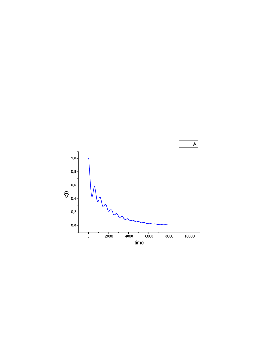
Figure D.1. Spontaneous emission of light from an atom. The figure presents a numerical solution for some artificial values of various parameters. The presence of oscillations at short times accompanied by decay for large times appears to be a general feature of the model (the number of visible oscillations and the decay rate are parameter-dependent).

In order to investigate the concrete atomic emission processes we introduce atomic units. Formally this means that we set $e,m,\hbar$ equal to one and note that

• $r=1$ means $r=0.53\cdot 10^{-8}\ cm$ (N.Bohr radius),

• $E=1$ means $E=27.2\ eV$ (typical atomic ionization energies),

• $t=1$ means $t=2.4\cdot 10^{-17}\ s$ (typical atomic oscillation times),

• $c=137$ (result of the relation $e^{2}/\hbar c=1/137$).

With those units it is possible to investigate realistic systems. One realizes that the only non-trivial constant is the speed of light, ${\mathbf{c}}$ which appears only in the expression of the smeared two point function $S(t-s)$. We have

$$S(t-s)=\int\frac{d^{3}p}{2{\mathbf{c}}p}\ e^{-ip{\mathbf{c}}(t-s)}\left(\delta^{ij}-\frac{{\mathbf{p}}^{i}{\mathbf{p}}^{j}}{{\mathbf{p}}^{2}}\right)\ \overline{\chi_{i}({\mathbf{p}})}\chi_{j}({\mathbf{p}}).$$

It is not difficult to find the explicit expressions for $\chi_{j}({\mathbf{p}})$ in case of the harmonic oscillator or the hydrogen atom wave functions. The numerical analysis, however, stumbles upon the following difficulties:

• The typical, experimental, decay times in case of the $2P\rightarrow 1S$ transition are of the order of nanoseconds. Such a time corresponds to $10^{8}$ in atomic units. This raises the question of the propagation of the numerical errors.

• The appearance of the speed of light in the function $S(t-s)$ makes it both small and supported only for very short $|t-s|$. This even further worsens the problem, as the time step must be accordingly small.

Those difficulties, however, could have been anticipated from the very beginning: the model constructed here describes equally well the emission of X-rays from the atomic nuclei and the emission of rf radiation from the oscillatory levels of molecules. In terms of the decay times those processes are separated by a vast gap of more than ten orders of magnitude.

In the case of the hydrogen atom bound states $1S$ and $2P$ the smeared electromagnetic two-point function is:

$$S(d)=\frac{16\pi}{3{\mathbf{c}}}\int_{0}^{\infty}p\ dp\ e^{-ip\ d{\mathbf{c}}}\left[\frac{A^{2}-p^{2}}{(A^{2}+p^{2})^{3}}\right]^{2},$$

where $A=3/2$, all in atomic units.

The main merit of the model constructed above (apart from its well-defined mathematical status) lies in the appearance of the two-point function of the ”base” state of the radiation field on the right-hand side of equation (D.2). Thus, it is clear that the ”vacuum fluctuations” cause the decay of the atomic energy levels. Indeed it is relatively easy in the presented framework to investigate the spontaneous emission in the presence of a thermal state or a squeezed state of the radiation field.

For the latter type of states such an investigation may have important consequences, namely, it could clarify the issue why the squeezed states produce atomic spectra with lines narrower than the natural line width [PCK92].

Appendix E GNS construction and thermo-field dynamics

In the chapter devoted to the construction of representations of the CAR algebra $O\iota^{\prime}\acute{}\hskip 3.0pt$ we have indicated that interesting things occur, if the integral kernel $B$ of the two-point distribution $\omega$ is not a projection.

We shall consider a simple example of this here. Let $\mathcal{H}=\mathbb{C}^{2}$ and

$$B=\begin{pmatrix}1&0\\ 0&1/2\\ \end{pmatrix}.$$

If we look for the Gelfand ideal in the one-field operator subalgebra of $O\iota^{\prime}\acute{}\hskip 3.0pt$, we will find that

$$\psi\left[(\alpha,0)\right]$$

is the only (one-field) annihilation operator present there.

In order to obtain a representation of $O\iota^{\prime}\acute{}\hskip 3.0pt$ we may pretend that we have the creation/annihilation operators, as usual, with the vacuum:

$$a(\sqrt{B}f)\ \Omega =0,$$

$$b(\sqrt{1-B}f)\ \Omega =0,$$

but those operators will in general no longer be elements of $O\iota^{\prime}\acute{}\hskip 3.0pt$. In the standard Fock space built with the help of $a^{*},b^{*}$’s we may construct the representation of $O\iota^{\prime}\acute{}\hskip 3.0pt$ via

$$\psi(f)=a(\sqrt{B}f)+b^{*}(\sqrt{1-B}f).$$

The representation defined as above turns out, however, to be reducible; there are operators different from the identity which act in the representation space and commute with the representation of $O\iota^{\prime}\acute{}\hskip 3.0pt$ given above.

Much better insight into the nature of the problem is gained, if we extend $\mathcal{H}$ to $\mathcal{H}_{2}=\mathcal{H}\otimes\mathcal{H}$ and choose

$$B_{2}=\begin{pmatrix}B&\sqrt{B}\sqrt{1-B}\\ B\sqrt{1-B}&1-B\\ \end{pmatrix},$$

which is a projection operator on $\mathcal{H}_{2}$ irrespective of $B$. We shall now search for a representation of a doubled algebra generated by the elements $\Psi(f)$, $f\in\mathcal{H}_{2}$, and their adjoints. In our example

$$B_{2}=\begin{pmatrix}1&0&0&0\\ 0&1/2&0&1/2\\ 0&0&0&0\\ 0&1/2&0&1/2\\ \end{pmatrix}.$$

If we introduce an orthonormal basis of $\mathcal{H}_{2}$:

$$e =(1,0,0,0),$$

$$\tilde{e} =(0,0,1,0),$$

$$u =(0,1,0,1)/\sqrt{2},$$

$$v =(0,1,0,-1)/\sqrt{2}.$$

then

$$B_{2}=P_{e}+P_{u},$$

where $P$’s denote the respective 1-dimensional projections. The Gelfand ideal reveals four annihilation operators:

$$a_{1} =\Psi(e), b_{1} =\Psi^{*}(\tilde{e}),$$

$$a_{1} =\Psi(u), b_{1} =\Psi^{*}(v),$$

which obey the standard anti-commutation relations among themselves. An irreducible representation of the doubled algebra is thus given on the Fock space constructed with the help of the adjoints of the above operators. What is interesting is that on such a Hilbert space there acts also the representation $\pi(\hbox{$O\iota^{\prime}\acute{}\hskip 3.0pt$})$ of the original algebra $O\iota^{\prime}\acute{}\hskip 3.0pt$ with

$$\psi(f)\equiv\Psi[(f_{+},f_{-},0,0)]=f_{+}\ a_{1}+\frac{f_{-}}{\sqrt{2}}\ (a_{2}+b^{*}_{2}).$$

But in the representation space there act also the operators of the form

$$\tilde{\psi}(g)\equiv\Psi[(0,0,g_{+},g_{-}]=\frac{g_{-}}{\sqrt{2}}\ (a_{2}-b^{*}_{2})+g_{+}\ b^{*}_{1}.$$

This field and also its adjoint anti-commute with the representation of $O\iota^{\prime}\acute{}\hskip 3.0pt$. Thus, the observables constructed with their help all commute with the elements of $\pi(\hbox{$O\iota^{\prime}\acute{}\hskip 3.0pt$})$.

The doubling of $\mathcal{H}$ (and in turn of $O\iota^{\prime}\acute{}\hskip 3.0pt$) is frequently done in the literature on ”thermo field dynamics”. Further discussion of the representation theory constructed on a thermal two-point function can be found in [Ha96] chapter V.1.4 , or [Fre99].

Bibliography

- [AB65] A.I. Akhiezer, and V.B. Berestetski, Quantum electrodynamics, Interscience Publishers, 1965.
- [Ara71] H. Araki, On quasifree states of CAR and Bogoliubov automorphisms, Publ. RIMS Kyoto Univ. 6 (1970/71), 385–442.
- [BFS99] V. Bach, J.Fröhlich and I.M. Sigal, Spectral analysis for systems of atoms and molecules coupled to the quantized radiation field, Commun. Math. Phys. 207 (1999), 249
- [Ble50] K. Bleuler, Eine neue Methode zur Behandlung der longitudinalen und skalaren Photonen, Helv. Phys. Acta 23 (1950), 567.
- [BLP82] V.B. Berestetski, E.M. Lifshitz, and L.P. Pitaevskii, Quantum electrodynamics, vol 4. of Landau and Lifshitz’s course of theoretical physics, Pergamon Press, 1982.
- [BF00] R. Brunetti, and K. Fredenhagen, Microlocal analysis and interacting quantum field theories: Renormalization on physical backgrounds, Commun. Math. Phys. 208 (2000), 623 and www.arXiv.org math-ph (2000), 9903028.
- [BFV01] R. Brunetti, K. Fredenhagen, and R.Verch, The generally covariant locality principle - a new paradigm for local quantum field theory, www.arXiv.org math-ph (2001), 0112041.
- [Deh90] H. Dehmelt, Experiments with an isolated subatomic particle at rest, Rev. Mod. Phys. 62 (1990), 525.
- [DB60] B. DeWitt and R. Brehme, Radiation damping in gravitational field, Ann. Phys. 9 (1960), 220.
- [DM75] H.G. Dosch, and V.F. Müller, Renormalization of QED in an arbitrary strong time independent external field, Fort. Phys. 23 (1975), 661.
- [FV01] C. Fewster, and R.Verch A quantum weak energy inequality for Dirac fields in curved spacetime, Commun. Math. Phys. 225, 331 (2002) and www.arXiv.org math-ph (2001), 0105027.
- [Fe03] C. Fewster, Quantum energy inequalities and the Casimir effect, Notes from a talk given at DESY, June (2003).
- [Fre99] K. Fredenhagen, Quantenfeldtheorie in gekrümmter Raumzeit, Notes from a lecture held at Hamburg University, available at www.desy.de/uni-th/lqp, SS 1999.
- [Fre94] K. Fredenhagen, Superselection sectors, Notes from a lecture held at Hamburg University, available at www.desy.de/uni-th/lqp, WS 1994.
- [Fri74] F. G. Friedlander, The wave equation on a curved spacetime, Cambridge University Press, 1974.
- [GZ80] J.-L. Gervais, and D.Zwanziger, Derivation of the long range QED from the first principles, Phys. Lett. B94 (1980), 389.
- [Gup50] S.N. Gupta, The theory of longitudinal photons in quantum electrodynamics, Proc. Phys. Soc. A63 (1950), 681.
- [Ha96] R. Haag, Local quantum physics: fields, particles, algebras, 2-nd ed., Springer, 1996.
- [HC66] D. Hilbert and R. Courant, Methods of mathematical physics, vol. 2, Interscience Publishers, 1966.
- [Hol99] S. Hollands, The Hadamard condition for Dirac fields and adiabatic states on Robertson-Walker spacetimes, Commun. Math. Phys. 216, 635 (2001) and www.arXiv.org gr-qc (1999), 9906076.
- [HW1] S. Hollands, and R.M. Wald, Local Wick polynomials and time ordered products of quantum fields in curved spacetime, Commun. Math. Phys. 223, 289 www.arXiv.org gr-qc (2001), 0103074.
- [HW2] S. Hollands, and R.M. Wald, Existence of local covariant time ordered products of quantum fields in curved spacetime, www.arXiv.org gr-qc (2001), 0111108.
- [IZ78] C. Itzykson and J.-B. Zuber, Quantum field theory, McGraw-Hill, 1978.
- [Ju02] W. Junker, Erratum, Rev. Math. Phys. 14 no. 5 (2002), 511.
- [Ka00] K. Kartzert, Singularity structure of the two-point function of the free Dirac field on a globally hyperbolic spacetime , Annalen Phys. 9 (2000), 475, available at www.desy.de/uni-th/lqp.
- [KRW97] B. Kay, M.J.Radzikowski, and R.M. Wald, QFT on spacetimes with a compactly generated Cauchy horizon, Commun. Math. Phys. 183 (1997), 533, www.arXiv.org gr-qc , 9603012.
- [Ma02] P. Marecki, On the application of quantum inequalities to quantum optics, Phys. Rev. A 66, 053801, www.arXiv.org quant-ph (2002), 0203027.
- [Ma01] P. Marecki, Electrons at TESLA will experience thermal radiation, Notes from a talk given at the GrK meating in Cracow, (2001).
- [Mi01] S.V. Milton et al., Exponential gain and saturation of a Self-Amplified Spontaneous Emission Free-Electron Laser, Science 292 (2001), 2037.
- [MPS98] P. Mohr, G.Plunien, and G.Soff QED corrections in heavy atoms, Phys. Rep. 293 (1998), 228.
- [Mor01] V. Moretti, Comments on the stress-energy tensor operator in curved spacetime, www.arXiv.org gr-qc (2001), 0109048.
- [PCK92] E.S. Polzik, J.Carri, and H.J. Kimble, Spectroscopy with squeezed light, Phys. Rev. Lett. 68(20) (1992), 3020.
- [PS70] R.T. Powers and E. Störmer, Free states of the canonical anticommutation relations, Commun. Math. Phys. 16 (1970), 1.
- [Ra96] M.J. Radzikowski, Micro-local approach to the Hadamard condition in quantum field theory on curved space-time, Commun. Math. Phys. 179 (1996), 529.
- [RS75] M. Reed, and B. Simon Methods of modern mathematical physics II, Academic Press, 1975.
- [Ru77] S.N.M. Ruijsenaars, Charged particles in external fields. I. Classical theory, J. Math. Phys. 18 (1977), 720.
- [SV1] H. Sahlmann, and R. Verch, Passivity and microlocal spectrum condition, Commun. Math. Phys. 214, 705, www.arXiv.org math-ph (2000), 0002021.
- [SV2] H. Sahlmann, and R. Verch, Microlocal spectrum condition and Hadamard form for vector valued quantum fields in curved spacetime, Rev. Math. Phys. 13, 1203, www.arXiv.org math-ph (2001), 0008029.
- [Sch96] G. Scharf, Finite quantum electrodynamics, Springer, 1996.
- [SZ97] M.O. Scully, and M.S.Zubairy Quantum optics, Cambridge, 1997.
- [Sha02] V.M. Shabaev, Two-time Green’s function method in QED of high-Z few-electrons atoms, Phys. Rep. 356 (2002), 121.
- [SS65] D. Shale and W.F. Stinespring, Spinor representations of infinite orthogonal groups, J. Math. Mech. 14 (1965), 315.
- [Stö98] Th.Stöhlker, et. al., Charge-exchange cross section and beam lifetimes for stored and decelerated bare uranium ions, Phys. Rev. A58 (1998), 2043.
- [Tay95] M.E. Taylor, Partial differential equations, vol. 2, Springer, 1995.
- [Tha91] B. Thaller, The Dirac equation, Springer, 1991.
- [Ver94] R. Verch, Local definiteness, primarity and quasiequivalence of quasifree Hadamard quantum states in curved spacetime, Commun. Math. Phys. 160 (1994), 507
- [Wa94] R.M. Wald, Quantum field theory in curved spacetime and black hole thermodynamics, University of Chicago Press, 1994.
- [Web02] J.K. Webb, et. al., Further evidence for cosmological evolution of the fine structure constant, Phys. Rev. Lett. 87 (2002), 091301.
- [Wi01] C.M. Will, The confrontation between General Relativity and experiment, Living Rev. Relativity 4 (2001), 4; www.livingreviews.org/Articles/Volume4/2001-4will/.
Index
- Bogoliubov transformation §II.2.3
- Canonical anti-commutation relations §II.3.2
-
Causality
- of time-ordered products §VI.1
- Charge conjugation §II.3.1
- Current operator §VI.7.1
- Dirac field operator Definition II.8
-
Dirac operator
- self-adjointness Theorem II.1, Theorem II.2
- Essential spectrum §II.1.1
- Fock space §II.3.2
- Fock-Krein space §III.1
- GNS construction §II.2.2
- Ground state §II.3.4
- Gupta-Bleuler method Chapter III
-
Hilbert space
- transversal §III.2
- Krein adjoint §III.1
- Krein space §III.1
- Locality §VI.3.1
- Parametrix
- Polarization vectors §III.1
- Quasi-equivalence §II.2.3
- Rescaling transformations Definition VI.13
- Shale-Stinespring criterion Theorem II.5
- Wick expansion §VI.1
- Wick product §VI.6.3