Abstract

Boundary interactions of closed-string with open-strings are examined intended to provide a constructive formulation of boundary string field theory. As an illustration, we consider the BPS $D$-brane of the type II superstring in a constant NS-NS two-form background, and study the boundary interaction with arbitrary configurations of gauge field on the brane. The boundary interaction is presented, within the world-sheet cut-off theories, as an off-shell boundary state in the closed-string Hilbert space. It is regarded as a closed-string theoretical counterpart of the Wilson loop in the world-volume gauge theory. We show that the action of the closed-string BRST operator on the boundary state is translated into the non-linear BRST transformation of the open-string fields on the world-volume. In particular, the BRST invariance condition at the $\alpha^{\prime}$-order becomes the non-linear equation of motion for the non-commutative gauge theory. The action of the closed-string BRST operator on the boundary state is also shown to be identified with the beta functions of the world-sheet renormalization group flow.

1 Introduction and Summary

Boundary string field theory (BSFT) [1] has been proposed as a background independent formulation of open-string field theory and exploited in [2],[3],[4],[5]. The configuration space of open-string fields is identified with the space of two-dimensional field theories with arbitrary interactions on the boundary and a fixed conformal invariant world-sheet action in the bulk. An odd-symplectic structure on the space of the open-string fields is given by the two-point functions of the world-sheet theories with the boundary interactions. A nilpotent fermionic vector field is introduced as a certain limit of the bulk BRST operator. The string field action is determined from the above vector field and the odd-symplectic structure by using the Batalin-Vilkovisky formalism. However, the original construction of [1] is purely formal. Due to the short-distance divergences of the world-sheet theories, an introduction of the space of the boundary interactions and the odd-symplectic structure requires some regularization procedure. There is also an ambiguity in the definition of the nilpotent vector field and the notion of the classical equation of motion in the BSFT is still not clear.

In this paper, we will clarify these issues and make the first-step towards a constructive formulation of the BSFT. The aim of the present work are to provide a concrete construction of the boundary interactions within the cut-off theory, and to illustrate how the classical open-string interactions are extracted from the boundary interactions which are described in the world-sheet theory terminology. In order to be explicit, we will consider the BPS $D$-branes of the type II superstring theory in a constant NS-NS two-form background, and investigate the boundary interactions with the off-shell gauge fields on the branes.

The first quantization of open-string becomes intractable when the superconformal invariance of the world-sheet theory is broken on the boundary. However, if not broken in the bulk, the closed-string theory is quantized still in the conformal field theoretical method, and the boundary state formalism [6] developed in [7] will provide an appropriate framework for the description of the boundary interactions. The relevant boundary states are the states which do not satisfy the Ishibashi conditions (more precisely, the closed-string BRST invariance). In section 2 we construct the boundary states with arbitrary numbers of gluons. The resultant boundary states correctly include the open-string interactions, and reproduce the corresponding open-string one-loop amplitudes. Our construction in this paper is limited to the closed-string NS-NS sector. This is sufficient to see the classical physics of the open-string NS sector (disk amplitudes of gluons), which is dealt with by the NS-NS sector.

The boundary interaction of closed-string with arbitrary configurations of the gauge field on the brane is obtained from the above boundary states. In section 3, the boundary interaction is constructed in the closed-string Hilbert space by integrating the gluon boundary states over the moduli spaces of the path-ordered points on the boundary and summing them over the number of the gluons. The UV divergences of the open-string interactions arise when the gluon vertices collide with one another on the boundary. We will therefore make a point-splitting regularization by restricting the integrations over the moduli spaces so that intervals between any two gluon vertices on the boundary can not be less than a small cut-off parameter $\epsilon$. We also modify the path-ordering procedure to respect the global world-sheet supersymmetry, following to [8]. It is observed in [8] that the global world-sheet supersymmetry controls the short-distance divergences of the world-sheet theories. The resultant boundary state is denoted by $\bigl{|}W_{\epsilon}[A];\eta\bigr{\rangle}_{tot}$. It represents the boundary interaction with the off-shell gauge field on the brane. For another approach to the boundary interaction, see [9].

In the loop space approach to string field theory [10], the interactions are introduced by adding the string field vertices to the string field action. While, in BSFT, the interactions of the open-string fields should be extracted from the world-sheet boundary interaction. In section 4, we will overview the mechanism. We investigate the action of the closed-string BRST operator $Q_{c}$ on $\bigl{|}W_{\epsilon}[A];\eta\bigr{\rangle}_{tot}$. The use of the closed-string BRST operator is required by the background independence. Since the closed-string BRST operator does not include any coupling of the open-strings, the BRST invariance condition formally leads the linearized equation of motion for the gluons. However, the action of the closed-string BRST operator on the gluon vertices includes total-derivative terms. With the above point-splitting regularization, the total-derivative terms do not vanish in the integrals and contribute as the boundary terms of the regularized moduli space. These boundary terms turn out to provide the non-linear BRST transformation of the open-string fields. The zero of this non-linear BRST transformation gives the non-linear equation of motion. In this course, the leading contribution of each boundary term becomes too singular at $\epsilon\rightarrow 0$. Typically it behaves as $\sim 1/\epsilon$. The origin is the propagation of the open-string unphysical particles [11]. These unpleasant terms turn out to cancel with the contact terms which are brought about by the supersymmetric path-ordering procedure. The leading contributions are cancelled, and the next-to-leading contributions, which describe the propagation of the gluons, become the non-linear corrections to the BRST transformation and the equation of motion.

In the constant NS-NS two-form background, it is known [12] that the gauge field $A_{\mu}(x)$ on the brane acquires the non-commutativity and that the equation of motion for the gauge field becomes non-linear:

$$G^{\mu\nu}\nabla_{\mu}F_{\nu\rho}(x)=0\;,$$ (1.1)

where $\nabla_{\mu}$ and $F_{\mu\nu}$ are the covariant derivative and the field strength of the non-commutative gauge theory. In section 5, we compute the BRST invariance condition of the world-sheet boundary interaction at the $\alpha^{\prime}$-order and confirm that the condition $Q_{c}\bigl{|}W_{\epsilon}[A];\eta\bigr{\rangle}_{tot}=0$ leads to the non-linear equation of motion (1.1). We would notice that the above mechanism to extract the non-linear equation of motion is not restricted to the present non-commutative case. It can be easily generalized to the non-abelian Yang-Mills equation by associating the Chan-Paton factors with the gluon vertices.

In the original attempts to formulate string field theory as a theory of “all two-dimensional quantum field theories”, it was suggested in [13] that the classical equation of motion for string fields is given by the renormalization group equation of the world-sheet theories. In section 6, the boundary interaction is examined from the perspective of the world-sheet renormalization group. In our boundary state formulation, the beta functions of the boundary couplings $A_{\mu}(k)$ are defined by the following condition:

$$\int{d}^{p+1}k\;\beta_{A_{\mu}(k)}\frac{\delta}{\delta{A}_{\mu}(k)}\;\Bigl{|}\;W_{\epsilon}[A];\eta\;\Bigr{\rangle}_{tot}=-\epsilon\frac{\partial}{\partial\epsilon}\;\Bigl{|}\;W_{\epsilon}[A];\eta\;\Bigr{\rangle}_{tot}\;.$$ (1.2)

They become linear if the $\epsilon$-dependence of the regularized moduli spaces is neglected. By taking account of the $\epsilon$-dependence of the regularized moduli spaces, the beta functions turn to acquire the non-linearity:

$$\beta_{A_{\mu}(k)}=\alpha^{\prime}\int\frac{d^{p+1}x}{(2\pi)^{\frac{p+1}{2}}}e^{-ik\cdot{x}}G^{\nu\rho}\nabla_{\nu}F_{\rho\mu}(x)+{\cal O}(\alpha^{\prime 2})\;.$$ (1.3)

These beta functions coincide with the non-linear BRST transformations of the open-string fields. Therefore the action of $Q_{c}$ on $\bigl{|}W_{\epsilon}[A];\eta\bigr{\rangle}_{tot}$ is identified with the beta functions. This provides a concrete definition of the nilpotent vector field in the Batalin-Vilkovisky formulation of the BSFT. Gauge structure of the BSFT can be also studied from our approach. It will be reported elsewhere [14].

Finally, we comment on a possible extension of our formulation of the classical BSFT to the quantum BSFT. The quantum open-string theory inevitably contains the closed-string degrees of freedom. The resultant string field theory is an open-closed string field theory in which the closed-string interactions are encoded in the closed-string field vertices while the open-string interactions are encoded in the boundary states $\bigl{|}W_{\epsilon}[A];\eta\bigr{\rangle}_{tot}$. The equation of motion for $A_{\mu}(x)$ is deformed from $Q_{c}\bigl{|}W_{\epsilon}[A];\eta\bigr{\rangle}_{tot}=0$ by the closed-string interaction, and becomes to contain the interaction between $\bigl{|}W_{\epsilon}[A];\eta\bigr{\rangle}_{tot}$. From the space-time viewpoint, the boundary states $\bigl{|}W_{\epsilon}[A];\eta\bigr{\rangle}_{tot}$ correspond to the Wilson loops of the gauge theory on the branes. The deformed equation of motion may be the string theoretical realization of the loop equation of the gauge theory, and the closed-string BRST operator $Q_{c}$ corresponds to the loop Laplacian [15]. We hope that the progress along this line will shed light on the issues of the open-closed string duality.

2 Gluons in Closed-String Theory

In the present section, we make a description of the open-string degrees of freedom on a non-commutative D-brane in terms of the boundary state formalism. Our study is restricted to the massless particles in the open-string theory - gluons, and the closed-string NS-NS sector.

This section has two parts. As a set-up, boundary states without any open-string leg are briefly reviewed in the first subsection . In the second subsection, we construct boundary states with arbitrary numbers of gluons, with the method developed in [7]. The resultant boundary states by themselves capture the open-string tree interactions. The tree propagation between the boundary states correctly reproduce the open-string one-loop amplitudes. The BRST invariance of the boundary state with one-gluon leads to the linearized equation of motion for the gluon.

2.1 A brief review of boundary states without open-string vertices

Let us consider type II superstring theory with a non-commutative D$p$-brane. The case of even $p$ corresponds to the type IIA theory, while odd $p$ corresponds to the type IIB theory. We will use $\mu,\nu=0,1,2,\dotsc,p$ to denote the world-volume directions of the D$p$-brane, $i,j=p+1,p+2,\dotsc,9$ to denote the transverse directions of the brane and $M,N=0,1,2,\dotsc,9$ for the whole space-time indices. Closed strings couple to a constant space-time metric $g_{MN}$ with $g_{\mu{i}}=0$ and a constant two-form gauge field $B_{\mu\nu}$ in the bulk. The world-sheet action is given by

$$\begin{split}S=\frac{i}{2\pi}\int_{\Sigma}dw\wedge d\bar{w}\Bigl{[}\;&\frac{1}{\alpha^{\prime}}\bigl{\{}g_{MN}\partial_{w}X^{M}\partial_{\bar{w}}X^{M}-2\pi\alpha^{\prime}B_{\mu\nu}\partial_{w}X^{\mu}\partial_{\bar{w}}X^{\nu}\bigr{\}}\\ &+\frac{1}{2}g_{MN}\psi^{M}\partial_{\bar{w}}\psi^{N}+\frac{1}{2}g_{MN}\bar{\psi}^{M}\partial_{w}\bar{\psi}^{N}\;\Bigr{]}\;.\end{split}$$ (2.1)

Here we use the cylinder coordinates $w=\tau+i\sigma,\bar{w}=\tau-i\sigma$ ($\tau\!\geq\!0,\;0\!\leq\!\sigma\!\leq\!2\pi$) and the world-sheet $\Sigma$ has a boundary at $\tau=0$. We impose the boundary conditions

$$\begin{split}&E_{\mu\nu}\partial_{w}X^{\nu}+E_{\mu\nu}^{T}\partial_{\bar{w}}X^{\nu}\bigr{|}_{\tau=0}=0\;,\quad X^{i}\bigr{|}_{\tau=0}=x_{0}^{i}\;,\\ &E_{\mu\nu}\psi^{\nu}-i{\eta}E_{\mu\nu}^{T}\bar{\psi}^{\nu}\bigr{|}_{\tau=0}=0\;,\quad\psi^{i}+i\eta\bar{\psi}^{i}\bigr{|}_{\tau=0}=0\qquad(\eta=\pm 1)\;,\end{split}$$ (2.2)

where $E_{\mu\nu}=g_{\mu\nu}+2\pi\alpha^{\prime}B_{\mu\nu}$ and $E_{\mu\nu}^{T}=g_{\mu\nu}-2\pi\alpha^{\prime}B_{\mu\nu}$.

In the NS-NS sector, the world-sheet variables $X^{M}$, $\psi^{M}$ and $\bar{\psi}^{M}$ have the following mode-expansions:

$$X^{M}(\tau,\sigma)=\hat{x}^{M}-i\alpha^{\prime}\hat{p}^{M}\tau+i\sqrt{\frac{\alpha^{\prime}}{2}}\sum_{n\neq{0}}\Bigl{\{}\;\frac{\alpha^{M}_{n}}{n}e^{-n(\tau+i\sigma)}+\frac{\bar{\alpha}^{M}_{n}}{n}e^{-n(\tau-i\sigma)}\;\Bigr{\}}\;,$$ (2.3)

$$\psi^{M}(\tau,\sigma)=\sum_{r\in\mathbb{Z}+\frac{1}{2}}\psi^{M}_{r}e^{-r(\tau+i\sigma)},\quad\bar{\psi}^{M}(\tau,\sigma)=\sum_{r\in\mathbb{Z}+\frac{1}{2}}\bar{\psi}^{M}_{r}e^{-r(\tau-i\sigma)}\;.$$ (2.4)

The first quantization of the closed-string is achieved by imposing the following commutation relations:

$$\begin{split}&[x^{M},p^{N}]=ig^{MN},\quad[\alpha_{m}^{M},\alpha_{n}^{N}]=[\bar{\alpha}^{M}_{m},\bar{\alpha}^{N}_{n}]=g^{MN}m\delta_{m,-n}\;,\\ &\{\psi^{M}_{r},\psi_{s}^{N}\}=\{\bar{\psi}^{M}_{r},\bar{\psi}^{N}_{s}\}=g^{MN}\delta_{r,-s}\;,\end{split}$$ (2.5)

with all the other commutators equal to zero.

In the closed-string channel, the boundary conditions (2.2) are encoded in the boundary state $|B;\eta\rangle_{m}$ , which is defined by the following overlap conditions:

$$\begin{split}&\hat{p}^{\mu}|B;\eta\rangle_{m}=(\hat{x}^{i}-x_{0}^{i})|B;\eta\rangle_{m}=0\;,\\ &(E_{\mu\nu}\alpha_{n}^{\nu}+E^{T}_{\mu\nu}\bar{\alpha}_{-n}^{\nu})|B;\eta\rangle_{m}=(\alpha_{n}^{i}-\bar{\alpha}_{-n}^{i})|B;\eta\rangle_{m}=0\;,\qquad\mathrm{for}\quad n\neq 0\;,\\ &(E_{\mu\nu}\psi^{\nu}_{r}-i{\eta}E_{\mu\nu}^{T}\bar{\psi}_{-r})|B;\eta\rangle_{m}=(\psi^{i}_{r}+i\eta\bar{\psi}^{i}_{-r})|B;\eta\rangle_{m}=0\;,\qquad\mathrm{for}\quad r\in\mathbb{Z}+\frac{1}{2}\;.\end{split}$$ (2.6)

By using the above overlap conditions, we can easily check that the boundary state $|B;\eta\rangle_{m}$ satisfies the Ishibashi conditions

$$\bigl{(}L_{n}^{m}-\bar{L}_{-n}^{m}\bigr{)}|B;\eta\rangle_{m}=0\;,\quad\bigl{(}G_{r}^{m}+i{\eta}\bar{G}_{-r}^{m}\bigr{)}|B;\eta\rangle_{m}=0\;,$$ (2.7)

where $L_{n}^{m}$, $\bar{L}_{n}^{m}$ and $G_{r}^{m}$, $\bar{G}_{r}^{m}$ are the Virasoro and super Virasoro generators of the ($X$,$\psi$,$\bar{\psi}$) CFT respectively. An explicit form of $|B;\eta\rangle_{m}$ is given by $|B;\eta\rangle_{m}=Cg_{\eta}|x_{0}^{i}\rangle_{m}$, where

$$C=\biggl{\{}\frac{\det(E^{T}g^{-1}E)_{\mu\nu}}{(2\alpha^{\prime})^{p+1}}\biggr{\}}^{\frac{1}{4}}\biggl{\{}\frac{(2\pi^{2}\alpha^{\prime})^{9-p}}{\det{g_{ij}}}\biggr{\}}^{\frac{1}{4}}\;,$$ (2.8)

$$g_{\eta}=\prod_{n=1}^{\infty}\exp\Bigl{\{}-\frac{1}{n}N_{\mu\nu}\alpha_{-n}^{\mu}\bar{\alpha}^{\nu}_{-n}+\frac{1}{n}g_{ij}\alpha_{-n}^{i}\bar{\alpha}^{j}_{-n}\Bigr{\}}\prod_{r=1/2}^{\infty}\exp\Bigl{\{}i{\eta}N_{\mu\nu}\psi_{-r}^{\mu}\bar{\psi}_{-r}^{\nu}-i{\eta}g_{ij}\psi^{i}_{-r}\bar{\psi}^{j}_{-r}\Bigr{\}}\;,$$ (2.9)

$$|x_{0}^{i}\rangle_{m}=\int\frac{d^{9-p}k}{\sqrt{(2\pi)^{9-p}}}e^{ik_{i}(\hat{x}^{i}-x_{0}^{i})}|0\rangle_{m}\;.$$ (2.10)

Here $N_{\mu\nu}=\bigl{(}g\frac{1}{E}E^{T}\bigr{)}_{\mu\nu}$ and $|0\rangle_{m}$ is the $SL(2,\mathbb{C})$ invariant vacuum of the ($X$, $\psi$, $\bar{\psi}$) CFT. The normalization factor $C$ is determined by factorizing open-string annulus partition function in the closed-string channel.

The complete boundary state is obtained by tensoring $|B;\eta\rangle_{m}$ with states for the conformal ghosts $b,c,\bar{b},\bar{c}$ and for the superconformal ghost $\beta,\gamma,\bar{\beta},\bar{\gamma}$ :

$$|B;\eta\rangle_{tot}=|B;\eta\rangle_{m}\otimes|B\rangle_{gh}\otimes|B;\eta\rangle_{sgh}\;.$$ (2.11)

The boundary states $|B\rangle_{gh}$ and $|B;\eta\rangle_{sgh}$ are given by

$$|B\rangle_{gh} =\prod_{n=1}^{\infty}\exp\Bigl{\{}c_{-n}\bar{b}_{-n}+\bar{c}_{-n}b_{-n}\Bigr{\}}\Bigl{(}\frac{c_{0}+\bar{c}_{0}}{2}\Bigr{)}c_{1}\bar{c}_{1}|0\rangle_{gh}\;,$$ (2.12)

$$|B;\eta\rangle_{sgh} =\prod_{r=1/2}^{\infty}\exp\Bigl{\{}i\eta\bigl{(}\gamma_{-r}\bar{\beta}_{-r}-\bar{\gamma}_{-r}\beta_{-r}\bigr{)}\Bigr{\}}|-1,-1\rangle_{sgh}\;,$$ (2.13)

where $|0\rangle_{gh}$ is the $SL(2,\mathbb{C})$ invariant vacuum of the conformal ghost system and $|-1,-1\rangle_{sgh}$ is the ground state of the superconformal ghost system in the ($-1$,$-1$) picture. The mode operators of the ghost and superghost systems satisfy the following commutation relations:

$$\begin{split}\{c_{m},b_{n}\}&=\{\bar{c}_{m},\bar{b}_{n}\}=\delta_{m,-n}\;,\\ [\gamma_{r},\beta_{s}]&=[\bar{\gamma}_{r},\bar{\beta}_{s}]=\delta_{r,-s}\;,\end{split}$$ (2.14)

with all the other commutators equal to zero. The boundary states $|B\rangle_{gh}$ and $|B;\eta\rangle_{sgh}$ enjoy the overlap conditions

$$\begin{split}(c_{n}+\bar{c}_{-n})|B\rangle_{gh}&=(b_{n}-\bar{b}_{-n})|B\rangle_{gh}=0\;,\\ (\gamma_{r}+i\eta\bar{\gamma}_{-r})|B;\eta\rangle_{sgh}&=(\beta_{r}+i\eta\bar{\beta}_{-r})|B;\eta\rangle_{sgh}=0\;.\end{split}$$ (2.15)

Combining these conditions with the Ishibashi conditions (2.7), one can easily check that the complete boundary state $|B;\eta\rangle_{tot}$ is annihilated by the closed-string BRST operator

$$\begin{split}Q_{c}=&-\sum_{n\in\mathbb{Z}}c_{-n}L^{m}_{n}+\frac{1}{2}\sum_{r\in\mathbb{Z}+1/2}\gamma_{-r}G^{m}_{r}+\frac{1}{2}\sum_{m,n\in\mathbb{Z}}(m-n):c_{-m}c_{-n}b_{m+n}:\\ &\quad-\sum_{n\in\mathbb{Z}}\sum_{r\in\mathbb{Z}+1/2}\bigl{(}\frac{n}{2}-r\bigr{)}:c_{-n}\gamma_{-r}\beta_{n+r}:+\frac{1}{4}\sum_{r,s\in\mathbb{Z}}:\gamma_{-r}\gamma_{-s}b_{r+s}:\\ &\quad\quad+\Bigl{\{}\mathrm{anti-chiral{\;\;}part}\Bigr{\}}\;.\end{split}$$ (2.16)

The boundary state (2.11) depends on the value of $\eta$. The GSO projection of the closed-string theory selects a specific combination of the two values of $\eta=\pm 1$. In the NS-NS sector, the GSO projection operator is defined by

$$P_{GSO}=\frac{1+(-1)^{N_{\psi}+G_{sgh}}}{2}\frac{1+(-1)^{\bar{N}_{\psi}+\bar{G}_{sgh}}}{2}\;,$$ (2.17)

where $N_{\psi}$ and $G_{sgh}$ are the fermion number operator and the superghost number operator:

$$N_{\psi}=\sum_{r=1/2}^{\infty}g_{MN}\psi^{M}\psi^{N}\;,\quad G_{sgh}=-\sum_{r=1/2}^{\infty}(\gamma_{-r}\beta_{r}+\beta_{-r}\gamma_{r})-1\;,$$ (2.18)

and similarly for $\bar{N}_{\psi}$ and $\bar{G}_{sgh}$ of the anti-chiral sector. The GSO projection operator (2.17) acts on the boundary state $|B;\eta\rangle_{tot}$ as follows:

$$P_{GSO}|B;\eta\rangle_{tot}=\frac{1}{2}\bigl{\{}\;|B;\eta\rangle_{tot}-|B;-\eta\rangle_{tot}\bigr{\}}\;.$$ (2.19)

In the absence of any open-string leg, boundary states in the R-R sector are also constructed in [16].

2.2 Boundary states with gluons

We now construct the boundary states which describe the gauge field living on the D-brane. For a while, our attention will be concentrated on the matter part. It is convenient to introduce the one-dimensional superspace notation. Let $\theta$ be an anti-commuting coordinate on the world-sheet boundary. The one-dimensional superspace consists of the pair ($\sigma$, $\theta$). The superfield and the superderivative are defined by

$$\mathbf{X}^{\mu}=X^{\mu}-i\sqrt{\frac{\alpha^{\prime}}{2}}\theta\bigl{(}\psi^{\mu}+i\eta\bar{\psi}^{\mu}\bigr{)}\;,\quad D_{\theta}=\frac{\partial}{\partial\theta}-i\theta\frac{\partial}{\partial\sigma}\;.$$ (2.20)

Let $k_{\mu}$ and $A_{\mu}(k)$ be the momentum and polarization vectors. We begin with the following auxiliary operator:

$$:\exp\Bigl{\{}ik_{\mu}\mathbf{X}^{\mu}+{\lambda}A_{\mu}(k)D_{\theta}\mathbf{X}^{\mu}\Bigr{\}}:\;,$$ (2.21)

where $\lambda$ is an anti-commuting auxiliary parameter [17]. By expanding the auxiliary operator (2.21) in powers of $\lambda$, we get analogues of the open-string tachyon and gluon vertex operators as follows:

$$:\exp\Bigl{\{}ik_{\mu}\mathbf{X}^{\mu}+{\lambda}A_{\mu}(k)D_{\theta}\mathbf{X}^{\mu}\Bigr{\}}:\;=\;:e^{ik_{\mu}\mathbf{X}^{\mu}}:-i\lambda\Bigl{\{}\;i:A_{\mu}(k)D_{\theta}\mathbf{X}^{\mu}e^{ik_{\mu}\mathbf{X}^{\mu}}:\Bigr{\}}\;.$$ (2.22)

Let us overview how the operators in the closed-string theory describe the open-string interactions, with the help of the boundary state $|B;\eta\rangle_{m}$. The overlap conditions (2.6) say that the annihilation operators with respect to the boundary state $|B;\eta\rangle_{m}$ are

$$\begin{split}E_{\mu\nu}\alpha_{n}^{\nu}+E^{T}_{\mu\nu}\bar{\alpha}^{\nu}_{-n}\;,&\quad\alpha^{i}_{n}-\bar{\alpha}^{i}_{-n}\;,\quad n\in\mathbb{Z}\;,\\ E_{\mu\nu}\psi^{\nu}_{r}-i{\eta}E^{T}_{\mu\nu}\bar{\psi}^{\nu}_{-r}\;,&\quad\psi_{r}^{i}+i{\eta}\bar{\psi}^{i}_{-r}\;,\quad r\in\mathbb{Z}+\frac{1}{2}\;,\end{split}$$ (2.23)

rather than the lowering operators $\alpha^{M}_{n}$, $\bar{\alpha^{M}_{n}}$ ($n\geq 1$) and $\psi^{M}_{r}$, $\bar{\psi}^{M}_{r}$ ($r\geq 1/2$). Thus, for the operators acting on $|B;\eta\rangle_{m}$, the relevant normal-ordering operation is provided by placing all of the operators (2.23) to the right, and the relevant operator product expansion (OPE) is obtained by using this modified normal-ordering prescription. The modified normal-ordering and OPE reproduce the open-string interactions. For instance, the modified OPE between $\mathbf{X}^{\mu}$ becomes

$$\begin{split}&\mathbf{X}^{\mu}(0,\sigma_{1},\theta_{1})\mathbf{X}^{\nu}(0,\sigma_{2},\theta_{2})\\ &\sim\alpha^{\prime}G^{\mu\nu}\mathbf{G}(\sigma_{1},\theta_{1};\sigma_{2},\theta_{2})-\frac{i}{2}\theta^{\mu\nu}\mathrm{sign}(\sigma_{1}-\sigma_{2})+\frac{i}{2\pi}\theta^{\mu\nu}(\sigma_{1}-\sigma_{2})\;,\end{split}$$ (2.24)

where the tensors

$$G^{\mu\nu}=\frac{1}{2}\Bigl{(}\frac{1}{E}+\frac{1}{E^{T}}\Bigr{)}^{\mu\nu}\;,\quad\theta^{\mu\nu}=\pi\alpha^{\prime}\Bigl{(}\frac{1}{E}-\frac{1}{E^{T}}\Bigr{)}^{\mu\nu}$$ (2.25)

are the open-string metric and the non-commutative parameter respectively [12], and Green’s function on the superspace is defined by

$$\mathbf{G}(\sigma_{1},\theta_{1};\sigma_{2},\theta_{2})=-\ln|e^{i\sigma_{1}}-e^{i\sigma_{2}}|^{2}-i\theta_{1}\theta_{2}\frac{1}{\;\sin\bigl{(}{\frac{\sigma_{1}-\sigma_{2}}{2}}\bigr{)}\;}\;.$$ (2.26)

For dealing with the normal-ordering and the OPE with respect to $|B;\eta\rangle_{m}$, it becomes convenient to consider the Bogolubov transformation

$$O\quad\longmapsto\quad\widehat{O}=g_{\eta}^{-1}Og_{\eta}\;,$$ (2.27)

which maps the operators (2.23) to the lowering operators. Therefore, the normal-ordering of $O$ with respect to the boundary state $|B;\eta\rangle_{m}$ is translated to the normal-ordering of $\widehat{O}$ with respect to the $SL(2,\mathbb{C})$ invariant vacuum $|0\rangle_{m}$. The OPE between $O$ with respect to $|B;\eta\rangle_{m}$ is translated to the OPE between $\widehat{O}$ with respect to $|0\rangle_{m}$. We employ this description in the subsequent part of this paper.

We now return to the operator (2.21). Under the Bogolubov transformation (2.27), the auxiliary operator (2.21) transforms as

$$\begin{split}g_{\eta}^{-1}:\exp\Bigl{\{}ik_{\mu}\mathbf{X}^{\mu}&+{\lambda}A_{\mu}(k)D_{\theta}\mathbf{X}^{\mu}\Bigr{\}}:g_{\eta}\\ =R_{A}(\tau,\theta,\lambda;k)&\prod_{n=1}^{\infty}\exp\Bigl{\{}\sqrt{\frac{\alpha^{\prime}}{2}}\frac{1}{n}\bigl{(}k_{\mu}-i\lambda{\theta}nA_{\mu}(k)\bigr{)}(g^{-1}N^{T})^{\mu}_{\;\;\nu}\alpha_{-n}^{\nu}e^{-n(\tau-i\sigma)}\Bigr{\}}\\ \times&\prod_{n=1}^{\infty}\exp\Bigl{\{}\sqrt{\frac{\alpha^{\prime}}{2}}\frac{1}{n}\bigl{(}k_{\mu}+i\lambda{\theta}nA_{\mu}(k)\bigr{)}(g^{-1}N)^{\mu}_{\;\;\nu}\bar{\alpha}^{\nu}_{-n}e^{-n(\tau+i\sigma)}\Bigl{\}}\\ \times&\prod_{r=1/2}^{\infty}\exp\Bigl{\{}\sqrt{\frac{\alpha^{\prime}}{2}}\bigl{(}{\theta}k_{\mu}-i{\lambda}A_{\mu}(k)\bigr{)}(g^{-1}N^{T})^{\mu}_{\;\;\nu}\psi_{-r}^{\nu}e^{-r(\tau-i\sigma)}\Bigr{\}}\\ \times&\prod_{r=1/2}^{\infty}\exp\Bigl{\{}i\eta\sqrt{\frac{\alpha^{\prime}}{2}}\bigl{(}{\theta}k_{\mu}-i{\lambda}A_{\mu}(k)\bigr{)}(g^{-1}N)_{\;\;\nu}^{\mu}\bar{\psi}^{\nu}_{-r}e^{-r(\tau+i\sigma)}\Bigr{\}}\\ \times&:\exp\Bigl{\{}ik_{\mu}\mathbf{X}^{\mu}+{\lambda}A_{\mu}(k)D_{\theta}\mathbf{X}^{\mu}\Bigr{\}}:\;.\end{split}$$ (2.28)

The explicit form of the factor $R_{A}(\tau,\theta,\lambda;k)$ is given by

$$\begin{split}R_{A}(\tau,\theta,\lambda;k)=&\Bigl{(}1-e^{-2\tau}\Bigr{)}^{\frac{\alpha^{\prime}}{2}k_{\mu}(g^{-1}Ng^{-1})^{\mu\nu}k_{\nu}}\\ &\times\exp\Bigl{\{}-\frac{\alpha^{\prime}}{2}\lambda\theta f_{\mu\nu}(k)(g^{-1}Ng^{-1})^{\mu\nu}\frac{1}{1-e^{2\tau}}\Bigr{\}}\\ &\times\exp\Bigl{\{}+\frac{\alpha^{\prime}}{2}\lambda\theta f_{\mu\nu}(k)(g^{-1}Ng^{-1})^{\mu\nu}\frac{e^{\tau}}{1-e^{2\tau}}\Bigr{\}}\;,\end{split}$$ (2.29)

where $f_{\mu\nu}(k)=ik_{\mu}A_{\nu}(k)-ik_{\nu}A_{\mu}(k)$ is the Fourier transform of the field strength in the commutative gauge theory. The factor (2.29) has a singular behavior in the limit $\tau\rightarrow+0$. Thus, the action of the operator (2.21) on the boundary state $|B;\eta\rangle_{m}$ is singular at the world-sheet boundary. This is the consequence of the fact that operators have interactions with their mirror images through the existence of $|B;\eta\rangle_{m}$.

By subtracting the singular factor (2.29) from (2.21), we define the renormalized operator

$$\begin{split}W_{A}(\tau,\sigma,\theta,\lambda;k)=R_{A}^{-1}(\tau,\theta,\lambda;k)&\exp\Bigl{\{}-\frac{\alpha^{\prime}}{4}{\lambda\theta}f_{\mu\nu}(k)(g^{-1}Ng^{-1})^{\mu\nu}\Bigr{\}}\\ \times&:\exp\Bigl{\{}ik_{\mu}\mathbf{X}^{\mu}+\lambda{A_{\mu}(k)}D_{\theta}\mathbf{X}^{\mu}\Bigr{\}}:\;.\end{split}$$ (2.30)

The renormalized operators $\mathbf{V}_{tac}(\tau,\sigma,\theta;k)$ and $\mathbf{V}_{gl}^{\mu}(\tau,\sigma,\theta;k)$, corresponding to the open-string tachyon and gluon, are obtained by the following expansion of $W_{A}$ :

$$W_{A}(\tau,\sigma,\theta,\lambda;k)=\mathbf{V}_{tac}(\tau,\sigma,\theta;k)-i\lambda\;A_{\mu}(k)\mathbf{V}_{gl}^{\mu}(\tau,\sigma,\theta;k)\;.$$ (2.31)

An additional finite subtraction has been made in (2.30) by multiplying $\exp\bigl{\{}-\frac{\alpha^{\prime}}{4}\lambda\theta f_{\mu\nu}(g^{-1}Ng^{-1})^{\mu\nu}\bigr{\}}$. Similarly to the bosonic string case [7], this additional subtraction is necessary to reproduce the correct open-string one-loop amplitudes and the standard BRST action on the boundary state with one-gluon.

As a consequence of the fact that the action of (2.30) on the boundary state $|B;\eta\rangle_{m}$ is no longer singular at the world-sheet boundary, the operator

$$\widehat{W}_{A}(\sigma,\theta,\lambda;k)=\lim_{\tau\rightarrow+0}g_{\eta}^{-1}W_{A}(\tau,\sigma,\theta,\lambda;k)g_{\eta}\;,$$ (2.32)

is well-defined. In powers of the auxiliary parameter $\lambda$, the operator $\widehat{W}_{A}$ is expanded as

$$\widehat{W}_{A}(\sigma,\theta,\lambda;k)=\widehat{\mathbf{V}}_{tac}(\sigma,\theta;k)-i\lambda\;A_{\mu}(k)\widehat{\mathbf{V}}_{gl}^{\mu}(\sigma,\theta;k)\;.$$ (2.33)

The components $\widehat{\mathbf{V}}_{tac}(\sigma,\theta;k)$, $\widehat{\mathbf{V}}_{gl}^{\mu}(\sigma,\theta;k)$ are also obtained by making the Bogolubov transformation of $\mathbf{V}_{tac}(\tau,\sigma,\theta;k)$, $\mathbf{V}_{gl}^{\mu}(\tau,\sigma,\theta;k)$, and then taking the limit $\tau\rightarrow+0$. The OPE between $\widehat{W}_{A}$ takes the following form :

$$\begin{split}&\widehat{W}_{A}(\sigma_{1},\theta_{1},\lambda_{1};k^{(1)})\;\widehat{W}_{A}(\sigma_{2},\theta_{2},\lambda_{2};k^{(2)})\\ &=\exp\Bigl{\{}\;\frac{i}{2}k^{(1)}{\times}k^{(2)}\mathrm{sign}(\sigma_{1}-\sigma_{2})\Bigr{\}}\\ &\quad\times\exp\Bigl{\{}-\frac{i}{2\pi}k^{(1)}{\times}k^{(2)}(\sigma_{1}-\sigma_{2})\Bigr{\}}\\ &\quad\times\exp\Bigl{\{}\;\frac{i}{2\pi}\lambda_{1}\theta_{1}A(k^{(1)}){\times}k_{\nu}^{(2)}+\frac{i}{2\pi}\lambda_{2}\theta_{2}A(k^{(2)}){\times}k_{\nu}^{(1)}\Bigr{\}}\\ &\quad\times\exp\Bigl{[}\;\alpha^{\prime}G^{\mu\nu}\bigl{\{}ik^{(1)}_{\mu}+\lambda_{1}A_{\mu}(k^{(1)})D_{\theta_{1}}\bigr{\}}\bigl{\{}ik^{(2)}_{\nu}+\lambda_{2}A_{\nu}(k^{(2)})D_{\theta_{2}}\bigr{\}}\mathbf{G}(\sigma_{1},\theta_{1};\sigma_{2},\theta_{2})\Bigr{]}\\ &\;\quad\times:\widehat{W}_{A}(\sigma_{1},\theta_{1},\lambda_{1};k^{(1)})\;\widehat{W}_{A}(\sigma_{2},\theta_{2},\lambda_{2};k^{(2)}):\;,\end{split}$$ (2.34)

where we have employed the abbreviated notation : $k^{(\alpha)}{\times}k^{(\beta)}=k^{(\alpha)}_{\mu}\theta^{\mu\nu}k^{(\beta)}_{\nu}$, $k^{(\alpha)}{\times}A(k^{(\beta)})=k^{(\alpha)}_{\mu}\theta^{\mu\nu}A_{\nu}(k^{(\beta)})$. The appearance of the open-string metric $G^{\mu\nu}$ and the non-commutativity factor

$$\exp\bigl{\{}\;\frac{i}{2}k^{(1)}\times{k}^{(2)}\mathrm{sign}(\sigma_{1}-\sigma_{2})\bigr{\}}$$ (2.35)

in the OPE (2.34), implies that the operator (2.32) captures the open-string interactions [12]. From (2.34), we can check that the operators $\widehat{\mathbf{V}}_{tac}(\sigma,\theta;k)$ and $\widehat{\mathbf{V}}_{gl}^{\mu}(\sigma,\theta;k)$ in (2.33) satisfy the analogues of the OPEs between the tachyon and gluon vertices in the open-string theory with the constant $B_{\mu\nu}$ background. The factor

$$\begin{split}&\exp\Bigl{\{}-\frac{i}{2\pi}k^{(1)}{\times}k^{(2)}(\sigma_{1}-\sigma_{2})\Bigr{\}}\\ &\times\exp\Bigl{\{}\;\frac{i}{2\pi}\lambda_{1}\theta_{1}A(k^{(1)}){\times}k^{(2)}+\frac{i}{2\pi}\lambda_{2}\theta_{2}A(k^{(2)}){\times}k^{(1)}\Bigr{\}}\end{split}$$ (2.36)

in (2.34) looks like strange in the open-string interpretation. However, in the presence of this factor, we can correctly reproduce the open-string one-loop amplitudes of gluons. The factor (2.36) also plays an important role in the derivation of the supergravity couplings of non-commutative D-branes from the boundary state formalism [7, 14].

By expanding the superfield operators $\mathbf{V}_{tac}(\tau,\sigma,\theta;k)$ and $\mathbf{V}_{gl}^{\mu}(\tau,\sigma,\theta;k)$ in powers of $\theta$, we obtain two kinds of renormalized operators for the open-string tachyon and gluon respectively:

$$\mathbf{V}_{tac}(\tau,\sigma,\theta;k) =V^{(-1)}_{tac}(\tau,\sigma;k)+{\theta}V^{(0)}_{tac}(\tau,\sigma;k)\;,$$ (2.37)

$$\mathbf{V}_{gl}^{\mu}(\tau,\sigma,\theta;k) =V^{(-1)\mu}_{gl}(\tau,\sigma;k)+{\theta}V^{(0)\mu}_{gl}(\tau,\sigma;k)\;.$$ (2.38)

The operators $V_{tac}^{(-1)}(\tau,\sigma;k)$ and $V^{(-1)\mu}_{gl}(\tau,\sigma;k)$ correspond to the $-1$ picture vertex operators in the open-string theory, while $V_{tac}^{(0)}(\tau,\sigma;k)$ and $V^{(0)\mu}_{gl}(\tau,\sigma;k)$ correspond to the $0$ picture vertex operators. We employ the operators $V_{tac}^{(0)}(\tau,\sigma;k)$ and $V^{(0)\mu}_{gl}(\tau,\sigma;k)$ and integrate all positions of the vertices on the boundary. So we do not need to add any contribution of the ghosts and the superghosts to the vertices. This is relevant to compute the amplitudes for the annulus, in which the volume of the conformal Killing group is finite and the super-conformal Killing groups are absent.

The boundary state with a single open-string tachyon and the boundary state with a single gluon are obtained by acting $V_{tac}^{(0)}(\tau,\sigma;k)$ and $V^{(0)\mu}_{gl}(\tau,\sigma;k)$ on $|B;\eta\rangle_{m}$ respectively, and then by taking the limit $\tau\rightarrow+0$ :

$$\begin{split}|B_{tac};(\sigma;k);\eta\rangle_{tot}&\equiv\lim_{\tau\rightarrow+0}V_{tac}^{(0)}(\tau,\sigma;k)|B;\eta\rangle_{tot}\\ &=Cg_{\eta}\widehat{V}_{tac}^{(0)}(\sigma;k)|x^{i}_{0}\rangle_{m}\otimes|B\rangle_{gh}\otimes|B;\eta\rangle_{sgh}\;,\end{split}$$ (2.39)

$$\begin{split}|B[A];(\sigma;k);\eta\rangle_{tot}&\equiv\lim_{\tau\rightarrow+0}A_{\mu}(k)V_{gl}^{(0)\mu}(\tau,\sigma;k)|B;\eta\rangle_{tot}\\ &=Cg_{\eta}A_{\mu}(k)\widehat{V}_{gl}^{(0)\mu}(\sigma;k)|x^{i}_{0}\rangle_{m}\otimes|B\rangle_{gh}\otimes|B;\eta\rangle_{sgh}\;,\end{split}$$ (2.40)

where the operators $\widehat{V}^{(0)}_{tac}(\sigma;k)$ and $\widehat{V}^{(0)\mu}_{gl}(\sigma;k)$ are the components of the superfield operators $\widehat{\mathbf{V}}_{tac}(\sigma,\theta;k)$ and $\widehat{\mathbf{V}}^{\mu}_{gl}(\sigma,\theta;k)$ :

$$\widehat{\mathbf{V}}_{tac}(\sigma,\theta;k) =\widehat{V}^{(-1)}_{tac}(\sigma;k)+\theta\widehat{V}^{(0)}_{tac}(\sigma;k)\;,$$ (2.41)

$$\widehat{\mathbf{V}}_{gl}^{\mu}(\sigma,\theta;k) =\widehat{V}^{(-1)\mu}_{gl}(\sigma;k)+\theta\widehat{V}^{(0)\mu}_{gl}(\sigma;k)\;.$$ (2.42)

In (2.39) and (2.40), we include the ghost part $|B\rangle_{gh}$ and the superghost part $|B;\eta\rangle_{sgh}$. The states (2.39) and (2.40) depend on the value of $\eta$, through both the state $|B;\eta\rangle_{tot}$ and the operators $V_{tac}^{(0)}$, $V^{(0)\mu}_{gl}$. The closed-string GSO projection operator (2.17) projects out the one-tachyon state (2.39) :

$$P_{GSO}|B_{tac};(\sigma;k);\eta\rangle_{tot}=0\;,$$ (2.43)

and selects a specific combination of the one-gluon state $|B[A];(\sigma;k);\eta=\pm 1\rangle_{tot}$ :

$$P_{GSO}|B[A];(\sigma;k);\eta\rangle_{tot}=\frac{1}{2}\bigl{\{}\;|B[A];(\sigma;k);\eta\rangle_{tot}-|B[A];(\sigma;k);-\eta\rangle_{tot}\bigr{\}}\;,$$ (2.44)

respectively.

The boundary state with $N$ gluons is obtained by taking the same step as for $N=1$ :

$$\begin{split}&\bigl{|}B[A];(\sigma_{1},k^{(1)}),(\sigma_{2},k^{(2)}),\dotsc,(\sigma_{N},k^{(N)});\eta\bigr{\rangle}_{tot}\\ &\equiv\lim_{\tau_{\alpha}\rightarrow+0}V_{A}^{(0)}(\tau_{1},\sigma_{1};k^{(1)})V_{A}^{(0)}(\tau_{2},\sigma_{2};k^{(2)})\dots V_{A}^{(0)}(\tau_{N},\sigma_{N};k^{(N)})|B;\eta\rangle_{tot}\\ &\quad=C\;g_{\eta}\widehat{V}^{(0)}_{A}(\sigma_{1};k^{(1)})\widehat{V}^{(0)}_{A}(\sigma_{2};k^{(2)})\dots\widehat{V}^{(0)}_{A}(\sigma_{N};k^{(N)})|x_{0}^{i}\rangle_{m}\otimes|B\rangle_{gh}\otimes|B;\eta\rangle_{sgh}\;,\end{split}$$ (2.45)

where we adopt an abbreviated notation :

$$\mathbf{V}_{A}(\tau,\sigma,\theta;k) ={V}_{A}^{(-1)}(\tau,\sigma;k)+\theta{V}_{A}^{(0)}(\tau,\sigma;k)\equiv{A}_{\mu}(k)\mathbf{V}_{gl}^{\mu}(\tau,\sigma,\theta;k)\;,$$ (2.46)

$$\widehat{\mathbf{V}}_{A}(\sigma,\theta;k) =\widehat{{V}}_{A}^{(-1)}(\sigma;k)+\theta\widehat{{V}}_{A}^{(0)}(\tau,\sigma;k)\equiv{A}_{\mu}(k)\widehat{\mathbf{V}}_{gl}^{\mu}(\sigma,\theta;k)\;.$$ (2.47)

From the OPE (2.34), the $N$-gluons boundary state (2.45) by itself describes the open-string $N$-points tree amplitude. The GSO projection of the $N$-gluon boundary state (2.45) is given by the following combination :

$$\begin{split}\frac{1}{2}\Bigl{\{}\;&\bigr{|}B[A];(\sigma_{1},k^{(1)}),(\sigma_{2},k^{(2)}),\dotsc,(\sigma_{N},k^{(N)});\eta=+1\bigr{\rangle}_{tot}\\ &\quad\quad-\bigr{|}B[A];(\sigma_{1},k^{(1)}),(\sigma_{2},k^{(2)}),\dotsc,(\sigma_{N},k^{(N)});\eta=-1\bigl{\rangle}_{tot}\Bigr{\}}\;.\end{split}$$ (2.48)

The closed-string cylinder amplitudes in the NS-NS sector should reproduce the open-string one-loop amplitudes with the anti-periodic boundary condition in the time direction of the world-sheet. The dual boundary state with $N$ gluons ${}_{tot}\langle{B[A]};(\sigma_{1};k^{(1)}),\dotsc,(\sigma_{N};k^{(N)});\eta|$ is obtained from (2.45) by taking the Hermitian conjugation of it and flipping the sign of $\eta$. The tree propagations between the boundary states are given by

$$\begin{split}{}_{tot}\bigl{\langle}{B[A]};(\sigma_{N+1};k^{(N+1)})&,\dotsc,(\sigma_{N+M};k^{(N+M)});\eta^{\prime}\bigr{|}(c_{0}-\bar{c}_{0})\\ &\times(b_{0}+\bar{b}_{0})e^{-\tau_{(c)}(L_{0}^{tot}+\bar{L}_{0}^{tot})}\bigl{|}{B[A]};(\sigma_{1};k^{(1)}),\dotsc,(\sigma_{N};k^{(N)});\eta\bigr{\rangle}_{tot}\;,\end{split}$$ (2.49)

where $L_{0}^{tot}$ and $\bar{L}_{0}^{tot}$ are the Virasoro zero modes including the contributions of the ghosts and the superghosts, and $\tau_{(c)}$ is the length of the cylinder. The insertion $(c_{0}-\bar{c}_{0})$ is associated with the rotation of the cylinder, while the insertion $(b_{0}+\bar{b}_{0})$ is associated with the moduli of the cylinder $\tau_{(c)}$. By integrating (2.49) over $\sigma_{1},\dotsc,\sigma_{M+N}$ and $\tau_{(c)}$, we obtain the open-string $M+N$ annulus amplitude of the Ramond sector when $\eta\eta^{\prime}=+1$, while we obtain the open-string amplitudes of the NS sector when $\eta\eta^{\prime}=-1$, as we expect. The GSO-projected combination (2.48) gives the correct combination of the open-string one-loop amplitudes.

Linearized equation of motion from BRST invariance

In the closed-string field theory, an arbitrary string field is a vector in the closed-string Hilbert space, and the BRST invariance condition for it leads to the (linearized) equation of motion of the closed-string field theory. The gluon boundary states (2.40), (2.45) are also elements of the closed-string Hilbert space. Therefore, it is reasonable to expect that the BRST invariance condition for the boundary states with gluons leads to the equation of motion for the gluons.

Let us consider the BRST invariance condition for the one-gluon boundary state
$\oint{d\sigma}|B[A];(\sigma,k);\eta\rangle_{tot}$. When the vertex operators do not contain the ghosts and the superghosts, the overlap conditions for $|B\rangle_{gh}$ and $|B;\eta\rangle_{sgh}$ (2.15) implies that the action of the closed-string BRST operator (2.16) reduces to

$$Q_{c}\quad\sim\quad-\frac{1}{\;2\;}\sum_{n\in\mathbb{Z}}(c_{-n}-\bar{c}_{n})(L_{n}^{m}-\bar{L}_{-n}^{m})+\frac{1}{\;4\;}\!\!\sum_{r\in\mathbb{Z}+1/2}\!(\gamma_{-r}-i\eta\bar{\gamma}_{r})(G_{r}^{m}+i\eta\bar{G}_{-r}^{m})\;.$$ (2.50)

Thus, the BRST transformation of the one-gluon boundary state becomes as follows:

$$\begin{split}&Q_{c}\biggl{[}\int_{0}^{2\pi}d\sigma|B[A];(\sigma,k);\eta\rangle_{tot}\biggr{]}\\ &=\frac{C}{2}\int_{0}^{2\pi}d\sigma\;g_{\eta}\;\biggl{\{}\;-\sum_{n\in\mathbb{Z}}(c_{-n}-\bar{c}_{n})\bigl{[}\mathcal{L}_{n},\widehat{V}_{A}^{(0)}(\sigma;k)\bigr{]}\\ &\qquad\qquad\qquad\qquad+\frac{1}{\;2\;}\!\!\sum_{r\in\mathbb{Z}+1/2}(\gamma_{-r}-i\eta\bar{\gamma}_{r})\bigl{[}\mathcal{G}_{r},\widehat{V}_{A}^{(0)}(\sigma;k)\bigr{]}\;\biggr{\}}|x^{i}_{0}\rangle_{m}\otimes|B\rangle_{gh}\otimes|B;\eta\rangle_{sgh}\;,\end{split}$$ (2.51)

where $\mathcal{L}_{n}$, $\mathcal{G}_{r}$ are the Bogolubov transformations of the generators of the super-diffeomorphism on the boundary:

$$\mathcal{L}_{n}=g_{\eta}^{-1}(L_{n}^{m}-\bar{L}_{-n}^{m})g_{\eta}\;,\quad\mathcal{G}_{r}=g_{\eta}^{-1}(G_{r}^{m}+i\eta\bar{G}_{-r}^{m})g_{\eta}\;.$$ (2.52)

The commutation relations between the generators in (2.52) and the gluon vertex operators in (2.47) are as follows:

$$\begin{split}\;\bigl{[}\mathcal{L}_{n},\widehat{V}^{(0)}_{A}(\sigma;k)\bigr{]}&=-i\frac{d}{d\sigma}\bigl{\{}e^{in\sigma}\widehat{V}_{A}^{(0)}(\sigma;k)\bigr{\}}+\alpha^{\prime}\bigl{(}k\cdot{k}\bigr{)}ne^{in\sigma}\widehat{V}_{A}^{(0)}(\sigma;k)\\ &\qquad\qquad\qquad\qquad\qquad\qquad+\alpha^{\prime}\bigl{(}k\cdot{A}(k)\bigr{)}n^{2}e^{in\sigma}\widehat{V}_{tac}^{(-1)}(\sigma;k)\;,\end{split}$$ (2.53)

$$\begin{split}\bigl{[}\mathcal{G}_{r},\widehat{V}^{(0)}_{A}(\sigma;k)\bigr{]}&=-i\frac{d}{d\sigma}\bigl{\{}e^{ir\sigma}\widehat{V}_{A}^{(-1)}(\sigma;k)\bigr{\}}+2\alpha^{\prime}\bigl{(}k\cdot{k}\bigr{)}re^{ir\sigma}\widehat{V}_{A}^{(-1)}(\sigma;k)\\ &\qquad\qquad\qquad\qquad\qquad\qquad-2\alpha^{\prime}\bigl{(}k\cdot{A}(k)\bigr{)}re^{ir\sigma}\widehat{V}_{tac}^{(0)}(\sigma;k)\;,\end{split}$$ (2.54)

$$\bigl{[}\mathcal{L}_{n},\widehat{V}^{(-1)}_{A}(\sigma;k)\bigr{]} =-i\frac{d}{d\sigma}\bigl{\{}e^{in\sigma}\widehat{V}_{A}^{(-1)}(\sigma;k)\bigr{\}}+\bigl{(}\;\alpha^{\prime}k\cdot{k}-\frac{1}{2}\;\bigr{)}ne^{in\sigma}\widehat{V}_{A}^{(-1)}(\sigma;k)\;,$$ (2.55)

$$\bigl{\{}\mathcal{G}_{r},\widehat{V}^{(-1)}_{A}(\sigma;k)\bigr{\}} =e^{ir\sigma}\widehat{V}_{A}^{(0)}(\sigma;k)+2\alpha^{\prime}\bigl{(}k\cdot{A}(k)\bigr{)}re^{ir\sigma}\widehat{V}_{tac}^{(-1)}(\sigma;k)\;,$$ (2.56)

where we have abbreviated as $k\cdot{k}=k_{\mu}G^{\mu\nu}k_{\nu}$, $k\cdot{A}(k)=k_{\mu}G^{\mu\nu}A_{\nu}(k)$. By plugging (2.53) and (2.54) into (2.51), we obtain

$$\begin{split}&Q_{c}\biggl{[}\int_{0}^{2\pi}d\sigma|B[A];(\sigma,k);\eta\rangle_{tot}\biggr{]}\\ &=-\frac{iC}{2}\int^{2\pi}_{0}d\sigma\;\frac{d}{d\sigma}\Bigl{\{}-\sum_{n\in\mathbb{Z}}(c_{-n}-\bar{c}_{n})e^{in\sigma}\widehat{V}_{A}^{(0)}(\sigma;k)+\frac{1}{\;2\;}\!\!\sum_{r\in\mathbb{Z}+1/2}\!(\gamma_{-r}-i\eta\bar{\gamma}_{r})e^{ir\sigma}\widehat{V}_{A}^{(-1)}(\sigma;k)\Bigr{\}}\\ &\quad-C\int^{2\pi}_{0}d\sigma\int{d\theta}\;g_{\eta}\biggl{[}\;-\alpha^{\prime}\bigl{(}k\cdot{k}\bigr{)}A_{\mu}(k)D_{\theta}^{\;2}\mathbf{C}(\sigma,\theta)\widehat{\mathbf{V}}_{gl}^{\mu}(\sigma,\theta;k)\\ &\qquad\qquad\qquad\qquad\qquad\quad+\alpha^{\prime}\bigl{(}k\cdot{A}(k)\bigr{)}D^{\;3}_{\theta}\mathbf{C}(\sigma,\theta)\widehat{\mathbf{V}}_{tac}(\sigma,\theta;k)\;\biggr{]}\;|x^{i}_{0}\rangle_{m}\otimes|B\rangle_{gh}\otimes|B;\eta\rangle_{sgh}\;,\end{split}$$ (2.57)

where we have combined the ghosts and the superghosts into the superfield on the boundary

$$\mathbf{C}(\sigma,\theta)=\frac{\;1\;}{2}\Bigl{\{}\;\sum_{n\in\mathbb{Z}}\;(c_{-n}-\bar{c}_{n})\;e^{in\sigma}\;+\;\theta\!\!\sum_{r\in\mathbb{Z}+1/2}\!(\gamma_{-r}-i\eta\bar{\gamma}_{r})\;e^{ir\sigma}\;\Bigr{\}}\;.$$ (2.58)

Since the the total derivative term in (2.57) vanishes, the BRST transformation law of the single-gluon boundary state becomes

$$\begin{split}&Q_{c}\biggl{[}\int_{0}^{2\pi}d\sigma|B[A];(\sigma,k);\eta\rangle_{tot}\biggr{]}\\ &=\alpha^{\prime}\bigl{(}k\cdot{k}\bigr{)}A_{\mu}(k)\;C\int^{2\pi}_{0}\!d\sigma\int{d\theta}\;g_{\eta}\;D_{\theta}^{\;2}\mathbf{C}(\sigma,\theta)\widehat{\mathbf{V}}_{gl}^{\mu}(\sigma,\theta;k)|x^{i}_{0}\rangle_{m}\otimes|B\rangle_{gh}\otimes|B;\eta\rangle_{sgh}\\ &\quad-\alpha^{\prime}\bigl{(}k\cdot{A}(k)\bigr{)}\;C\int^{2\pi}_{0}\!d\sigma\int{d\theta}\;g_{\eta}\;D^{\;3}_{\theta}\mathbf{C}(\sigma,\theta)\widehat{\mathbf{V}}_{tac}(\sigma,\theta;k)|x^{i}_{0}\rangle_{m}\otimes|B\rangle_{gh}\otimes|B;\eta\rangle_{sgh}\;.\end{split}$$ (2.59)

Therefore, the BRST invariance condition of the single-gluon boundary state $\oint{d\sigma}|B[A];(\sigma;k);\eta\rangle_{tot}$ requires

$$\bigl{(}k\cdot{k}\bigr{)}A_{\mu}(k)=0\;,\quad k\cdot{A}(k)=0\;.$$ (2.60)

These are nothing but the linearized equation of motion and the Lorentz gauge condition for the gluon with the open-string metric $G^{\mu\nu}$.

It is enlightening to rewrite (2.59) from the string field theory viewpoint. In the string field theory, the world-sheet BRST transformation law for the vertex operators is translated into the target space BRST transformation law for the string fields. The equation (2.59) says that the world-sheet BRST transformation of the single-gluon boundary state becomes the linear combination of the boundary states with the vertices

$$\widehat{\mathbf{V}}^{\ast\mu}_{gl}(\sigma,\theta;k)=\Bigl{[}\;(D_{\theta}^{\;2}\mathbf{C})\widehat{\mathbf{V}}^{\mu}_{gl}\;\Bigr{]}(\sigma,\theta;k)\;,\quad\widehat{\mathbf{V}}_{a.g}(\sigma,\theta;k)=\Bigl{[}\;(D_{\theta}^{\;3}\mathbf{C})\widehat{\mathbf{V}}_{tac}\;\Bigr{]}(\sigma,\theta;k)\;.$$ (2.61)

Each coefficient in (2.59) is identified with the target space BRST transformation of the string fields which are associated with the vertices $\widehat{\mathbf{V}}^{\ast\mu}_{gl}(\sigma,\theta;k)$ and $\widehat{\mathbf{V}}_{a.g}(\sigma,\theta;k)$.

The open-string field theory in itself is equipped [18] with the structure of the Batalin-Vilkovisky formulation [19]. Due to the ghost-number anomaly, the inner-product in the open-string Hilbert space becomes the odd-symplectic form, and the anti-bracket is obtained from this odd-symplectic form. Each string field is paired with its antifield in accord with the anti-bracket. States which correspond to the vertices $\widehat{\mathbf{V}}^{\ast\mu}_{gl}(\sigma,\theta;k)$ and $\widehat{\mathbf{V}}_{a.g}(\sigma,\theta;k)$ can be found in the open-string Hilbert space. Since $D_{\theta}^{\;2}\mathbf{C}(\sigma,\theta)$ corresponds to the ghost zero-mode of the open-string theory, the state which corresponds to the vertex $\widehat{\mathbf{V}}^{\ast\mu}_{gl}(\sigma,\theta;k)$ must be paired with the state of the gluon vertex $\widehat{\mathbf{V}}^{\mu}_{gl}(\sigma,\theta;k)$. Therefore, the string field associated with the vertex operator $\widehat{\mathbf{V}}^{\ast\mu}_{gl}(\sigma,\theta;k)$ is the antifield for the gluon $A_{\mu}(k)$ . We denote it by $A_{\mu}^{\ast}(k)$. The string field which is associated with $\widehat{\mathbf{V}}_{a.g}(\sigma,\theta;k)$ is the target space antighost $\mathcal{B}(k)$. Both $A_{\mu}^{\ast}(k)$ and $\mathcal{B}(k)$ are the Grassmann-odd fields and have the ghost number $-1$. Each coefficient in (2.59) is identified with the target space BRST transformation of $A_{\mu}^{\ast}(k)$ and $\mathcal{B}(k)$ respectively. Therefore, (2.59) is rewritten as follows:

$$\begin{split}&Q_{c}\;\biggl{[}\;\int_{0}^{2\pi}\!d\sigma\int{d}\theta\;g_{\eta}\;A_{\mu}(k)\widehat{\mathbf{V}}_{gl}(\sigma,\theta;k)\;\biggr{]}\;|x^{i}_{0}\rangle_{m}\otimes|B\rangle_{gh}\otimes|B;\eta\rangle_{sgh}\\ &=-\int^{2\pi}_{0}d\sigma\int{d\theta}\;g_{\eta}\biggl{[}\;\delta_{\mathbf{B}}^{0}A_{\mu}^{\ast}(k)\widehat{\mathbf{V}}^{\ast\mu}_{gl}(\sigma,\theta;k)+\delta_{\mathbf{B}}^{0}\mathcal{B}(k)\widehat{\mathbf{V}}_{a.g}(\sigma,\theta;k)\;\biggr{]}\\ &\qquad\qquad\qquad\qquad\qquad\qquad\qquad\qquad\qquad\qquad\times|x^{i}_{0}\rangle_{m}\otimes|B\rangle_{gh}\otimes|B;\eta\rangle_{sgh}\;,\end{split}$$ (2.62)

where the target space BRST transformations are given by

$$\delta_{\mathbf{B}}^{0}A_{\mu}^{\ast}(k)=-\alpha^{\prime}\bigl{(}k\cdot{k}\bigr{)}A_{\mu}(k)\;,\quad\delta_{\mathbf{B}}^{0}\mathcal{B}(k)=\alpha^{\prime}\bigl{(}k\cdot{A}(k)\bigr{)}\;.$$ (2.63)

3 Boundary Interaction of Closed-String

In the previous section, we have constructed the boundary states with arbitrary numbers of the gluons. They reproduce the open-string amplitudes correctly. In this section, by using these boundary states, we describe the interaction with external gauge field as an element of the closed-string Hilbert space.

The boundary state with $N$-gluons (2.45) can be rewritten by means of the supersymmetric gluon vertices (2.47) as follows :

$$\begin{split}&\bigl{|}B[A];(\sigma_{1},k^{(1)}),\dotsc,(\sigma_{N},k^{(N)});\eta\bigr{\rangle}_{tot}\\ &=C\;g_{\eta}\int{d}\theta_{1}\widehat{\mathbf{V}}_{A}(\sigma_{1},\theta_{1};k^{(1)})\dots\int{d}\theta_{N}\widehat{\mathbf{V}}_{A}(\sigma_{N},\theta_{N};k^{(N)})|x^{i}_{0}\rangle_{m}\otimes|B\rangle_{gh}\otimes|B;\eta\rangle_{sgh}\;.\end{split}$$ (3.1)

One may expect that the closed-string state which represents the boundary interaction with the external gauge field

$$A_{\mu}(x)=\int\frac{d^{p+1}k}{(2\pi)^{\frac{p+1}{2}}}A_{\mu}(k)e^{ik\cdot{x}}$$ (3.2)

is obtained by integrating (3.1) over the momenta $k^{(1)},\dotsc,k^{(N)}$ and the position of the gluons $\sigma_{1},\dotsc,\sigma_{N}$, and then by summing it over $N=0,1,2,\dotsc,\infty$ :

$$\begin{split}&C\;g_{\eta}\sum_{N=0}^{\infty}i^{N}\int_{0}^{2\pi}\!d\sigma_{1}d\theta_{1}\widehat{\mathbf{V}}_{A}\bigl{(}\mathbf{X}(\sigma_{1},\theta_{1})\bigr{)}\cdots\int_{0}^{2\pi}\!d\sigma_{N}d\theta_{N}\widehat{\mathbf{V}}_{A}\bigl{(}\mathbf{X}(\sigma_{N},\theta_{N})\bigr{)}\\ &\qquad\qquad\qquad\qquad\qquad\qquad\times\prod_{\alpha=1}^{N-1}\Theta(\sigma_{\alpha+1}-\sigma_{\alpha})\;|x^{i}_{0}\rangle_{m}\otimes|B\rangle_{gh}\otimes|B;\eta\rangle_{sgh}\;,\end{split}$$ (3.3)

where $\Theta(\sigma)$ is the step function defined as $\Theta(\sigma)=1$ for $\sigma>0$ and $\Theta(\sigma)=0$ for $\sigma<0$. In (3.3), we have introduced the notation

$$\widehat{\mathbf{V}}_{A}\bigl{(}\mathbf{X}(\sigma,\theta)\bigr{)}=\int\frac{d^{p+1}k}{(2\pi)^{\frac{p+1}{2}}}\widehat{\mathbf{V}}_{A}(\sigma,\theta;k)\;.$$ (3.4)

However, due to the short-distance divergence of the boundary correlation functions (2.26), the state (3.3) is not a well-defined object, and needs some regularization procedure. We make a point-splitting regularization at the world-sheet boundary, by introducing a small positive cut-off parameter $\epsilon$ and replacing the step-functions $\Theta(\sigma_{\alpha+1}-\sigma_{\alpha})$ in (3.3) with the regularized ones $\Theta(\sigma_{\alpha+1}-\sigma_{\alpha}-\epsilon)$. In the cut-off theory, it is convenient to deal with the dimensionless couplings. The equation (2.53) says that the gluon vertex operator $\int{d\sigma}{d\theta}\widehat{\mathbf{V}}_{gl}^{\mu}(\sigma,\theta;k)$ has the scaling dimension $\alpha^{\prime}(k{\cdot}k)$. To make the couplings $A_{\mu}(k)$ dimensionless, we make the redefinition of the couplings as

$$A_{\mu}(k)\quad\longmapsto\quad\epsilon^{\alpha^{\prime}k\cdot{k}}A_{\mu}(k)\;,$$ (3.5)

and the vertex operators $\widehat{\mathbf{V}}_{A}(\sigma,\theta;k)$ and $\widehat{\mathbf{V}}_{A}\bigl{(}\mathbf{X}(\sigma,\theta)\bigr{)}$ are replaced with

$$\widehat{\mathbf{V}}_{A,\epsilon}(\sigma,\theta;k)=\epsilon^{\alpha^{\prime}k\cdot{k}}\widehat{\mathbf{V}}_{A}(\sigma,\theta;k)\;,\quad\widehat{\mathbf{V}}_{A,\epsilon}\bigl{(}\mathbf{X}(\sigma,\theta)\bigr{)}=\int\frac{d^{p+1}k}{(2\pi)^{\frac{p+1}{2}}}\widehat{\mathbf{V}}_{A,\epsilon}(\sigma,\theta;k)\;,$$ (3.6)

respectively. Instead of (3.3), we thus obtain

$$\begin{split}&C\;g_{\eta}\sum_{N=0}^{\infty}\frac{i^{N}}{N}\int_{0}^{2\pi}\!d\sigma_{1}d\theta_{1}\widehat{\mathbf{V}}_{A,\epsilon}\bigl{(}\mathbf{X}(\sigma_{1},\theta_{1})\bigr{)}\int_{-\infty}^{+\infty}\!\!d\sigma_{2}d\theta_{2}\widehat{\mathbf{V}}_{A,\epsilon}\bigl{(}\mathbf{X}(\sigma_{2},\theta_{2})\bigr{)}\\ &\qquad\qquad\qquad\qquad\qquad\qquad\times\cdots\times\int_{-\infty}^{+\infty}\!\!d\sigma_{N}d\theta_{N}\widehat{\mathbf{V}}_{A,\epsilon}\bigl{(}\mathbf{X}(\sigma_{N},\theta_{N})\bigr{)}\\ &\qquad\qquad\qquad\qquad\qquad\qquad\qquad\times\prod_{\alpha=1}^{N}\Theta(\sigma_{\alpha+1}-\sigma_{\alpha}-\epsilon)\;|x^{i}_{0}\rangle_{m}\otimes|B\rangle_{gh}\otimes|B;\eta\rangle_{sgh}\;.\end{split}$$ (3.7)

In the above expression (3.7), we formally extend the range of the coordinates $\sigma_{\alpha}$ ($\alpha=2,\dotsc,N$) to $-\infty\leq\sigma_{\alpha}\leq+\infty$ by using the $2\pi$ periodicity of the boundary state. We put $\sigma_{N+1}=\sigma_{1}+2\pi$. The singularity which arises when the two gluons at $\sigma_{1}$ and $\sigma_{N}$ collide has been regularized by inserting $\Theta(\sigma_{N+1}-\sigma_{N}-\epsilon)=\Theta(\sigma_{1}+2\pi-\sigma_{N}-\epsilon)$.

The state (3.7) is not invariant under the global world-sheet supersymmetry on the boundary : $\delta_{\xi}\sigma=i\xi\theta$, $\delta_{\xi}\theta=\xi$. The obstruction is the use of the step functions $\Theta(\sigma_{\alpha+1}-\sigma_{\alpha}-\epsilon)$ in the path-ordering procedure. Following to [8], we recover this global world-sheet supersymmetry by replacing $\sigma_{\alpha+1}-\sigma_{\alpha}$, the argument of the step functions in (3.7), with the supersymmetric invariant distances $\sigma_{\alpha+1}-\sigma_{\alpha}-i\theta_{\alpha}\theta_{\alpha+1}$. The supersymmetrized step functions

$$\begin{split}&\Theta(\sigma_{\alpha+1}-\sigma_{\alpha}-i\theta_{\alpha}\theta_{\alpha+1}-\epsilon)\\ &=\Theta(\sigma_{\alpha+1}-\sigma_{\alpha}-\epsilon)-i\theta_{\alpha}\theta_{\alpha+1}\delta(\sigma_{\alpha+1}-\sigma_{\alpha}-\epsilon)\;,\end{split}$$ (3.8)

introduce the contact terms in (3.7). It is observed in [8] that these contact terms exclude unpleasant divergences in the superstring amplitudes, and the global world-sheet supersymmetry on the boundary is also associated with the non-abelian gauge invariance of the effective theory.

With the point-splitting regularization and the supersymmetric path-ordering procedure, we finally obtain

$$\Bigl{|}\;W_{\epsilon}[A];\eta\;\Bigr{\rangle}$$

$$=\mathrm{SP}_{\epsilon}\biggl{[}\;C\;g_{\eta}\exp\Bigl{\{}\;i\oint{d\sigma}\int{d\theta}\;\widehat{\mathbf{V}}_{A,\epsilon}\bigl{(}\mathbf{X}(\sigma,\theta)\bigr{)}\;\Bigr{\}}\;\biggr{]}|x^{i}_{0}\rangle_{m}\otimes|B\rangle_{gh}\otimes|B;\eta\rangle_{sgh}$$

$$=C\;g_{\eta}\sum_{N=0}^{\infty}\frac{i^{N}}{N}\int^{2\pi}_{0}\!\!d\sigma_{1}{d}\theta_{1}\widehat{\mathbf{V}}_{A,\epsilon}\bigl{(}\mathbf{X}(\sigma_{1},\theta_{1})\bigr{)}\int^{+\infty}_{-\infty}\!\!d\sigma_{2}{d}\theta_{2}\widehat{\mathbf{V}}_{A,\epsilon}\bigl{(}\mathbf{X}(\sigma_{2},\theta_{2})\bigr{)}$$

$$\qquad\qquad\qquad\qquad\qquad\times\cdots\cdots\times\int^{+\infty}_{-\infty}\!\!d\sigma_{N}{d}\theta_{N}\widehat{\mathbf{V}}_{A,\epsilon}\bigl{(}\mathbf{X}(\sigma_{N},\theta_{N})\bigr{)}$$

$$\qquad\qquad\qquad\qquad\qquad\times\prod_{\alpha=1}^{N}\Theta(\sigma_{\alpha+1}-\sigma_{\alpha}-i\theta_{\alpha}\theta_{\alpha+1}-\epsilon)\;|x^{i}_{0}\rangle_{m}\otimes|B\rangle_{gh}\otimes|B;\eta\rangle_{sgh}$$

$$=C\;\sum_{N=0}^{\infty}\frac{i^{N^{2}}}{N}\int^{2\pi}_{0}\!\!{d}\sigma_{1}d\theta_{1}\int^{+\infty}_{-\infty}\!\!{d}\sigma_{2}d\theta_{2}\cdots\int^{+\infty}_{-\infty}\!\!{d}\sigma_{N}d\theta_{N}\prod_{\alpha=1}^{N}\Theta(\sigma_{\alpha+1}-\sigma_{\alpha}-i\theta_{\alpha}\theta_{\alpha+1}-\epsilon)$$

$$\qquad\qquad\times{g}_{\eta}\;\widehat{\mathbf{V}}_{A,\epsilon}\bigl{(}\mathbf{X}(\sigma_{1},\theta_{1})\bigr{)}\widehat{\mathbf{V}}_{A,\epsilon}\bigl{(}\mathbf{X}(\sigma_{2},\theta_{2})\bigr{)}\cdots\widehat{\mathbf{V}}_{A,\epsilon}\bigl{(}\mathbf{X}(\sigma_{N},\theta_{N})\bigr{)}|x^{i}_{0}\rangle_{m}\otimes|B\rangle_{gh}\otimes|B;\eta\rangle_{sgh}$$ (3.9)

where the symbol $\mathrm{SP}_{\epsilon}$ denotes the supersymmetric path-ordering operation with the cut-off parameter $\epsilon$. We put $(\sigma_{N+1},\theta_{N+1})=(\sigma_{1}+2\pi,-\theta_{1})$. We argue that the state (3.9) is the correct closed-string state which describes the boundary interaction with the gauge field. In section 4, we will confirm that the invariance condition of (3.9) under the closed-string BRST transformation leads the equation of motion for the non-commutative gauge theory. In particular, we will see that the supersymmetric path-ordering procedure controls the short-distance divergence of the world-sheet theory in the exquisite way.

From the space-time point of view, the state $\bigl{|}W_{\epsilon}[A]\bigr{\rangle}_{tot}$ is the closed-string theoretical counterpart of the Wilson loop. In the gauge theory, the basic gauge-invariant observables are provided by the Wilson loops . Therefore, the state $\bigl{|}W_{\epsilon}[A]\bigr{\rangle}_{tot}$ becomes the basic ingredient of the open-closed string field theory. In the sequel, we call the state (3.9) the Wilson loop.

4 Non-linear Equation of Motion from BRST Invariance

In this section we describe the BRST invariance condition of the Wilson loop. Let us first explain the origin of the non-linearity of the BRST transformation.

The Wilson loop consists of the boundary states of several numbers of gluons, where the gluon’s positions $(\sigma_{s},\theta_{s})$ are integrated over according to the supersymmetric path-ordering procedure (3.9). The action of the closed-string BRST operator on the Wilson loop is obtained from the collection of the actions on these boundary states of gluons. For the multi-gluon boundary states, computations of the actions of the closed-string BRST operator become more complicated than the single gluon boundary state. Let us consider the following state which appears in the non-supersymmetric path-ordered Wilson loop (3.7):

$$\frac{i^{N}}{N}C\int\!\prod_{\alpha=1}^{N}\frac{d^{p+1}k^{(\alpha)}}{(2\pi)^{\frac{p+1}{2}}}~{}g_{\eta}\int_{{\cal M}_{N,\epsilon}}\!\!\!d\sigma_{1}\wedge\cdots\wedge d\sigma_{N}\prod_{\beta=1}^{N}\widehat{V}_{A,\epsilon}^{(0)}(\sigma_{\beta};k^{(\beta)})$$

$$~{}~{}~{}~{}~{}~{}~{}~{}~{}~{}~{}~{}~{}~{}~{}~{}~{}~{}~{}~{}~{}~{}~{}~{}~{}\times|x_{0}^{i}\rangle_{m}\otimes|B\rangle_{gh}\otimes|B;\eta\rangle_{sgh}~{}.$$ (4.1)

In the supersymmetric path-ordered Wilson loop (3.9), the above state (4.1) arises as an element of the $N$-gluon boundary state. It is obtained from the $N$-gluon boundary state by integrating out all the anti-commuting coordinates $\theta_{\alpha}$ of the superfield operators $\widehat{{\bf V}}_{A,\epsilon}({\bf X}(\sigma_{\alpha},\theta_{\alpha}))$. The supersymmetrized step functions in the path-ordering procedure just contribute as the step functions $\Theta(\sigma_{\alpha+1}-\sigma_{\alpha}-\epsilon)$. The integration region ${\cal M}_{N,\epsilon}$ of the above integral is the configuration space of $\epsilon$-separated ordered $N$ points on the boundary circle. It consists of the $N$ points $(\sigma_{1},\cdots,\sigma_{N})$ which satisfy the conditions

$$0\leq\sigma_{1}<2\pi~{},~{}~{}~{}~{}~{}~{}~{}\sigma_{\alpha+1}-\sigma_{\alpha}\geq\epsilon~{}~{}~{}~{}(1\leq\alpha\leq N)~{}.$$ (4.2)

${\cal M}_{2,\epsilon}$ and ${\cal M}_{3,\epsilon}$ are depicted in Figures 1 and 2.

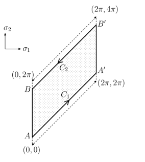
Figure 1: Configuration space $\mathcal{M}_{2,\epsilon}$ is the shaded parallelogram $AA^{\prime}B^{\prime}B$, where the two lines $\overline{AB}$ and $\overline{A^{\prime}B^{\prime}}$ are identified with each other. $A=(0,\epsilon)$, $B=(0,2\pi-\epsilon)$, $A^{\prime}=(2\pi,2\pi+\epsilon)$, $B^{\prime}=(2\pi,4\pi-\epsilon)$. The boundary of $\mathcal{M}_{2,\epsilon}$ consists of the two lines $C_{1}$ and $C_{2}$ . The parallelogram drawn by the dotted lines is the configuration space of the unregularized theory ($\epsilon=0$).

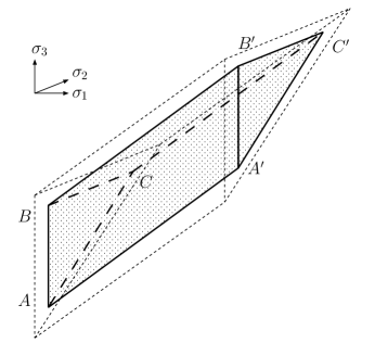
Figure 2: Configuration space $\mathcal{M}_{3,\epsilon}$ is the shaded triangular prism, where the two sides $ABC$ and $A^{\prime}B^{\prime}C^{\prime}$ are identified with each other. $A=(0,\epsilon,2\epsilon),\ B=(0,\epsilon,2\pi-\epsilon),\ C=(0,2\pi-2\epsilon,2\pi-\epsilon),\ A^{\prime}=(2\pi,2\pi+\epsilon,2\pi+2\epsilon),\ B^{\prime}=(2\pi,2\pi+\epsilon,4\pi-\epsilon),\ C^{\prime}=(2\pi,4\pi-2\epsilon,4\pi-\epsilon)$ The boundary of $\mathcal{M}_{3,\epsilon}$ consists of the three parallelograms $AA^{\prime}B^{\prime}B,\ CC^{\prime}A^{\prime}A,$ and $BB^{\prime}C^{\prime}C$. The triangular prism drawn by the dotted lines is the configuration space of the unregularized theory ($\epsilon=0$).

The action of the superconformal generators on the $N$-gluon boundary state can be computed by using the commutation relations (2.53)-(2.56) as in the case of the single gluon boundary state. However, the vanishings of the total derivative terms such as occurred for the single gluon boundary state do not happen in the present case since the boundary of the configuration space is not empty. For instance, let us consider the Virasoro action on the above state (4.1). The computation by using the commutation relation (2.53) gives rise to the following boundary integral:

$$\frac{i^{(N-1)}}{N}\int_{{\cal M}_{N,\epsilon}}d\sigma_{1}\wedge\cdots\wedge d\sigma_{N}\sum_{\alpha=1}^{N}\frac{d}{d\sigma_{\alpha}}\left\{e^{in\sigma_{\alpha}}\prod_{\beta=1}^{N}\widehat{V}_{A,\epsilon}^{(0)}(\sigma_{\beta};k^{(\beta)})\right\}$$

$$=\frac{i^{(N-1)}}{N}\int_{\partial{\cal M}_{N,\epsilon}}\sum_{\alpha=1}^{N}(-)^{\alpha-1}e^{in\sigma_{\alpha}}d\sigma_{1}\wedge\cdots\stackrel{{\scriptstyle\alpha}}{{\stackrel{{\scriptstyle\vee}}{{\cdot}}}}\cdots\wedge d\sigma_{N}\prod_{\beta=1}^{N}\widehat{V}_{A,\epsilon}^{(0)}(\sigma_{\beta};k^{(\beta)})~{}.$$ (4.3)

The boundary $\partial{\cal M}_{N,\epsilon}$ has several components. It can be written formally in the form $\partial{\cal M}_{N,\epsilon}=\cup_{\alpha=1}^{N}{\cal N}_{N,\epsilon}^{(\alpha)}$, where ${\cal N}_{N,\epsilon}^{(\alpha)}$ is the boundary component characterized by the condition $\sigma_{\alpha+1}=\sigma_{\alpha}+\epsilon$. For the case of $N=2$, the boundary components ${\cal N}_{2,\epsilon}^{(1)}$ and ${\cal N}_{2,\epsilon}^{(2)}$ are respectively the lines $C_{1}$ and $C_{2}$ in Figure 1. For the case of $N=3$, the boundary components ${\cal N}_{3,\epsilon}^{(1)}$, ${\cal N}_{3,\epsilon}^{(2)}$ and ${\cal N}_{3,\epsilon}^{(3)}$ are respectively the parallelograms $AA^{\prime}B^{\prime}B$, $CC^{\prime}A^{\prime}A$ and $BB^{\prime}C^{\prime}C$ in Figure 2. The integration in (4.3) becomes the sum of the integrations over the components ${\cal N}_{N,\epsilon}^{(\alpha)}$ of $\partial{\cal M}_{N,\epsilon}$. A typical configuration of the $N$ points on the boundary component ${\cal N}_{N,\epsilon}^{(\alpha)}$ is depicted in Figure 3. On this component, two gluons marked by $\alpha$ and $\alpha+1$ in the integral (4.3) are close to each other. They are thought to be in the open-string tree channel and their propagating modes are described by open-string vertex operators. Therefore the integral over this component becomes effectively the integral of the other gluons and the open-string vertex operator which describes the lightest propagating mode of the above two gluons. This indicates that boundary states with $N-1$ legs are brought about from the $N$-gluon boundary state by the action of the superconformal generators. This happens also for the action of the closed-string BRST operator and becomes the origin of the non-linearity. The configuration space ${\cal M}_{N,\epsilon}$ has corners when $N\geq 3$. The boundary components ${\cal N}_{N,\epsilon}^{(\alpha)}$ are patched together along the corners. For instance, ${\cal N}_{3,\epsilon}^{(\alpha)}$ are patched together along the lines $\overline{AA^{\prime}}$,$\overline{BB^{\prime}}$ and $\overline{CC^{\prime}}$ in Figure 2. On the tubular neighbourhoods of the corners, more than two gluons are thought to be in the open-string channel. Suitable modifications of the above argument are required there.

Figure 3: Typical configuration of $\mathcal{N}^{(\alpha)}_{N,\epsilon}$.

It becomes important to study the boundary states which are brought about effectively from the boundary integrals such as (4.3). In particular, we need to know the open-string vertex operator which describes the lightest propagating mode of the two gluons. This can be read from the expansion of the product of the $0$ picture gluon vertex operators. By using the OPE (2.34) we obtain

$$\widehat{V}^{(0)}_{A,\epsilon}(\sigma;k_{1})\widehat{V}^{(0)}_{A,\epsilon}(\sigma+\epsilon;k_{2})$$

$$=2\alpha^{\prime}\epsilon^{\alpha^{\prime}(k_{1}+k_{2})^{2}-2}(2\alpha^{\prime}k_{1}\cdot k_{2}-1)e^{-\frac{i}{2}k_{1}\times k_{2}}A(k_{1})\cdot A(k_{2})\widehat{V}_{tac}^{(-1)}(\sigma;k_{1}+k_{2})$$

$$~{}~{}~{}~{}+{\cal O}(\epsilon^{\alpha^{\prime}(k_{1}+k_{2})^{2}-1})~{}.$$ (4.4)

The operator $\widehat{V}_{tac}^{(-1)}$ in (4.4) is not the vertex operator of the open-string tachyon which is excluded by the GSO projection. It is rather the vertex operator of an unphysical open-string particle with $\alpha^{\prime}(\mathrm{mass})^{2}=-1$. The equation (4.4) says that the unphysical open-string particles appear as the dominant contribution in the intermediate open-string channels. This means that the boundary integral (4.3) yields the boundary states with less legs which include the unphysical open-string particles.

However, the multi-gluon boundary states of the Wilson loop include states other than (4.1). These states are brought about by the supersymmetric path-ordering. They are induced from the $\delta$-functions $-i\theta_{\alpha}\theta_{\alpha+1}\delta(\sigma_{\alpha+1}-\sigma_{\alpha}-\epsilon)$ of the supersymmetric step functions and give the contact interactions between the $-1$ picture gluon vertex operators. For instance, the following states appear in the $N$-gluon boundary state:

$$\frac{i^{(N-1)}}{N}C\int\!\prod_{\beta=1}^{N}\frac{d^{p+1}k^{(\beta)}}{(2\pi)^{\frac{p+1}{2}}}~{}g_{\eta}\int_{{\cal N}_{N,\epsilon}^{(\alpha)}}\!d\sigma_{1}\wedge\cdots\!\!\!\stackrel{{\scriptstyle\alpha+1}}{{\stackrel{{\scriptstyle\vee}}{{\cdot}}}}\!\!\!\cdots\wedge d\sigma_{N}\widehat{V}_{A,\epsilon}^{(-1)}(\sigma_{\alpha};k^{(\alpha)})\widehat{V}_{A,\epsilon}^{(-1)}(\sigma_{\alpha}+\epsilon;k^{(\alpha+1)})$$

$$~{}~{}~{}~{}~{}~{}~{}~{}~{}~{}~{}~{}~{}~{}~{}~{}~{}~{}~{}~{}~{}~{}\times\prod_{\beta\neq\alpha,\alpha+1}^{N}\widehat{V}_{A,\epsilon}^{(0)}(\sigma_{\beta};k^{(\beta)})|x_{0}^{i}\rangle_{m}\otimes|B\rangle_{gh}\otimes|B;\eta\rangle_{sgh}~{},$$ (4.5)

for $1\leq\alpha\leq N$.

The action of the closed-string BRST operator on the multi-gluon boundary states are obtained by piecing together all the actions on their elements. The contact interactions of the $-1$ picture operators turn out to play important roles under this incorporation. For instance, the Virasoro action on the contact interaction of the state (4.5) modifies the previous description of the nearby two gluons on the boundary component ${\cal N}_{N,\epsilon}^{(\alpha)}$. We will see in section 5 that these two gluons are described by the following combination of the gluon vertex operators:

$$\widehat{V}_{A,\epsilon}^{(0)}(\sigma;k_{1})\widehat{V}_{A,\epsilon}^{(0)}(\sigma+\epsilon;k_{2})+\frac{i}{2}\widehat{V}_{A,\epsilon}^{(-1)}(\sigma;k_{1})\partial_{\sigma}\widehat{V}_{A,\epsilon}^{(-1)}(\sigma+\epsilon;k_{2})$$

$$~{}~{}-\frac{i}{2}\partial_{\sigma}\widehat{V}_{A,\epsilon}^{(-1)}(\sigma;k_{1})\widehat{V}_{A,\epsilon}^{(-1)}(\sigma+\epsilon;k_{2})~{}.$$ (4.6)

The above combination is named the contact term $\Delta_{A,\epsilon}^{(0)}(\sigma;k_{1},k_{2})$ in section 5. The $-1$ picture operators in (4.6) come from the contact interactions which are required by the supersymmetric path-ordering. The role of these operators could be stressed in comparison with (4.4). The expansion into the power series of $\epsilon$ can be calculated by making use of the OPE (2.34). It can be written in the following form:

$$\Delta_{A,\epsilon}^{(0)}(\sigma;k_{1},k_{2})=i\epsilon^{\alpha^{\prime}(k_{1}+k_{2})^{2}-1}\Biggl{\{}I_{\mu}(k_{1},k_{2})\widehat{V}_{gl}^{(0)\mu}(\sigma;k_{1}+k_{2})+{\cal O}(\epsilon)\Biggr{\}}~{},$$ (4.7)

where the tensor $I_{\mu}$ is given by

$$I_{\mu}(k_{1},k_{2})$$

$$=\alpha^{\prime}e^{-\frac{i}{2}k_{1}\times k_{2}}\Biggl{\{}(k_{1\mu}-k_{2\mu})A(k_{1})\cdot A(k_{2})-2k_{1}\cdot A(k_{2})A_{\mu}(k_{1})+2k_{2}\cdot A(k_{1})A_{\mu}(k_{2})\Biggr{\}}.$$ (4.8)

By comparing the expansion (4.7) with (4.4), we see that the unphysical open-string particle, which appears in the open-string channel of the product $\widehat{V}_{A,\epsilon}^{(0)}\widehat{V}_{A,\epsilon}^{(0)}$, is actually cancelled out with the leading term of the expansion of the $-1$ picture operators. The next-to-leading terms of these expansions are combined and form the $0$ picture gluon vertex operator in (4.7). $\mathcal{O}(\epsilon)$ term in (4.7) represents the massive modes of the open-string. These massive modes become irrelevant at the short distance $\epsilon\sim 0$.

The cancellations of the unphysical open-string particle such as in the above turn to occur when the superconformal generators act on the multi-gluon boundary states. Owing to these cancellations the gluon boundary states with less legs are brought about. These happen also for the action of the closed-string BRST operator. This means that the actions of the closed-string BRST operator on the multi-gluon boundary states change the actions on the gluon boundary states with less legs effectively. The modifications can be interpreted as corrections to the (linear) BRST transformation $\delta^{0}_{\mathbf{B}}A^{*}_{\mu}$. The first correction $\delta^{1}_{\mathbf{B}}A^{*}_{\mu}$, which is quadratic with respect to $A_{\mu}$, turns out to be given by the tensor $I_{\mu}$. It can be written by using the Moyal $\star$-product as follows:

$$\delta_{{\bf B}}^{1}A^{*}_{\mu}(k)=i\alpha^{\prime}\int\!\frac{d^{p+1}x}{(2\pi)^{\frac{p+1}{2}}}\,e^{-ik_{\mu}x^{\mu}}G^{\nu\rho}\Bigl{(}\partial_{\mu}A_{\nu}\star A_{\rho}-A_{\nu}\star\partial_{\mu}A_{\rho}$$

$$~{}~{}~{}~{}~{}~{}~{}~{}~{}~{}~{}~{}~{}~{}~{}~{}~{}~{}~{}~{}~{}~{}~{}~{}~{}~{}~{}~{}~{}~{}~{}~{}~{}~{}~{}~{}~{}~{}~{}~{}~{}~{}~{}~{}~{}~{}~{}+2A_{\nu}\star\partial_{\rho}A_{\mu}-2\partial_{\nu}A_{\mu}\star A_{\rho}\Bigr{)}(x)~{},$$ (4.9)

where $A_{\mu}(x)=\int\frac{d^{p+1}k}{(2\pi)^{\frac{p+1}{2}}}e^{ik\cdot x}A_{\mu}(k)$ is the gauge field on the non-commutative world-volume. The non-linear BRST transformation, which we call $\delta_{\mathbf{B}}$, is obtained by putting together these corrections; $\delta_{\mathbf{B}}=\sum_{L=0}^{\infty}\delta_{\mathbf{B}}^{L}$. The $L$-th correction $\delta_{\mathbf{B}}^{L}\ (L\geq 1)$ generates polynomials of $A_{\mu}$ with the degree equal to $L+1$. We will compute the first two corrections $\delta_{\mathbf{B}}^{1}$ and $\delta_{\mathbf{B}}^{2}$ in section 5. Together with $\delta_{\mathbf{B}}^{0}$, they become the leading term of the $\alpha^{\prime}$-expansion of the non-linear transformation $\delta_{\mathbf{B}}$.

Let us describe the result: The action of the closed-string BRST operator on the Wilson loop has the form,

$$Q_{c}\times\textrm{SP}_{\epsilon}\Biggl{[}\,C\,g_{\eta}\exp\left\{i\oint d\sigma d\theta\>\widehat{\mathbf{V}}_{A,\epsilon}\bigl{(}\mathbf{X}(\sigma,\theta)\bigr{)}\Biggr{\}}\right]|x^{i}_{0}\rangle_{m}\otimes|B\rangle_{gh}\otimes|B;\eta\rangle_{sgh}$$ (4.10)

$$=-\textrm{SP}_{\epsilon}\Biggl{[}\,C\,g_{\eta}\ i\oint d\sigma d\theta\int\!\frac{d^{p+1}k}{(2\pi)^{\frac{p+1}{2}}}\>\epsilon^{\alpha^{\prime}k\cdot k}\biggl{\{}\delta_{\mathbf{B}}A^{*}_{\mu}(k)\,\widehat{\mathbf{V}}_{gl}^{*\mu}(\sigma,\theta;k)+\delta_{\mathbf{B}}\mathcal{B}(k)\,\widehat{\mathbf{V}}_{a.g}(\sigma,\theta;k)\biggr{\}}$$

$$~{}~{}~{}~{}~{}~{}~{}~{}~{}~{}~{}~{}~{}~{}~{}~{}~{}~{}~{}~{}~{}\times\exp\Biggl{\{}i\oint d\sigma d\theta\>\widehat{\mathbf{V}}_{A,\epsilon}\bigl{(}\mathbf{X}(\sigma,\theta)\bigr{)}\Biggr{\}}\Biggr{]}|x^{i}_{0}\rangle_{m}\otimes|B\rangle_{gh}\otimes|B;\eta\rangle_{sgh},$$

where

$$\delta_{\mathbf{B}}A^{*}_{\mu}(k) = \alpha^{\prime}\int\frac{d^{p+1}x}{(2\pi)^{\frac{p+1}{2}}}\>e^{-ik\cdot x}G^{\nu\rho}\nabla_{\rho}F_{\nu\mu}\Big{|}_{\partial\cdot A=0}(x)+\mathcal{O}(\alpha^{\prime\,2}),$$ (4.11)

$$\delta_{\mathbf{B}}\mathcal{B}(k) = \alpha^{\prime}\,k\cdot A(k)~{}~{}~{}~{}\biggl{(}=\delta^{0}_{\mathbf{B}}\mathcal{B}(k)\biggr{)}.$$ (4.12)

Here $\nabla_{\mu}=\partial_{\mu}+iA_{\mu}$ is the covariant derivative of the non-commutative gauge theory and $F_{\mu\nu}=\partial_{\mu}A_{\nu}-\partial_{\nu}A_{\mu}+iA_{\mu}\star A_{\nu}-iA_{\nu}\star A_{\mu}$ is the field strength. Therefore the BRST invariance of the Wilson loop requires the conditions, $\delta_{\mathbf{B}}A^{*}_{\mu}(k)=0$ and $\delta_{\mathbf{B}}\mathcal{B}(k)=0.$ These are respectively the equation of motion for the non-commutative gauge theory in the Lorentz gauge and the Lorentz gauge condition.

5 Derivation of the Result

In this section we provide a proof of the result stated in section 4. It is convenient to use the language of the superspace formalism. Let $S=(\sigma,\theta)$ be the superspace coordinate. The supersymmetric step function is denoted by $\Theta(S,S^{\prime})=\Theta(\sigma^{\prime}-\sigma-i\theta\theta^{\prime})$. We write the regularized multiple-ordered integrals in the Wilson loop (3.9) as follows:

$$\int_{{\cal I}_{N}(\epsilon)}\bigl{[}d^{N}S\bigr{]}=\int_{0}^{2\pi}\!\!d\sigma_{1}d\theta_{1}\int_{-\infty}^{+\infty}\!\!d\sigma_{2}d\theta_{2}\cdots\int_{-\infty}^{+\infty}\!\!d\sigma_{N}d\theta_{N}\prod_{\alpha=1}^{N}\Theta(S_{\alpha}+\epsilon,S_{\alpha+1})~{},$$ (5.1)

where $\bigl{[}d^{N}S\bigr{]}=dS_{1}\cdots dS_{N}$ with the $(1,1)$-superforms $dS_{\alpha}=d\sigma_{\alpha}d\theta_{\alpha}$. In the above we have introduced the supermoduli ${\cal I}_{N}(\epsilon)$ to represent the integration region of the RHS. We express the multi-gluon boundary states of the Wilson loop in the following form:

$$\frac{i^{N^{2}}}{N}C\int_{{\cal I}_{N}(\epsilon)}\bigl{[}d^{N}S\bigr{]}~{}g_{\eta}\widehat{{\bf V}}_{A,\epsilon}({\bf X}(S_{1}))\cdots\widehat{{\bf V}}_{A,\epsilon}({\bf X}(S_{N}))|x_{0}^{i}\rangle_{m}\otimes|B\rangle_{gh}\otimes|B;\eta\rangle_{sgh}~{}.$$ (5.2)

The action of the closed-string BRST operator on the Wilson loop is the collection of the actions on the multi-gluon boundary states. These actions can be written as

$$Q_{c}\times\frac{i^{N^{2}}}{N}C\int_{{\cal I}_{N}(\epsilon)}\bigl{[}d^{N}S\bigr{]}~{}g_{\eta}\widehat{{\bf V}}_{A,\epsilon}({\bf X}(S_{1}))\cdots\widehat{{\bf V}}_{A,\epsilon}({\bf X}(S_{N}))|x_{0}^{i}\rangle_{m}\otimes|B\rangle_{gh}\otimes|B;\eta\rangle_{sgh}$$

$$=\sum_{\alpha=1}^{N}\pm\frac{i^{N^{2}}}{N}C\int_{{\cal I}_{N}(\epsilon)}\bigl{[}d^{N}S\bigr{]}~{}g_{\eta}\widehat{{\bf V}}_{A,\epsilon}({\bf X}(S_{1}))\cdots\delta\widehat{{\bf V}}_{A,\epsilon}({\bf X}(S_{\alpha}))\cdots\widehat{{\bf V}}_{A,\epsilon}({\bf X}(S_{N}))$$

$$~{}~{}~{}~{}~{}~{}~{}~{}~{}~{}~{}~{}~{}~{}~{}~{}~{}~{}~{}~{}~{}~{}~{}~{}~{}~{}~{}~{}~{}~{}~{}~{}~{}~{}~{}~{}~{}~{}~{}~{}~{}\times|x_{0}^{i}\rangle_{m}\otimes|B\rangle_{gh}\otimes|B;\eta\rangle_{sgh}~{},$$ (5.3)

where $\delta\widehat{{\bf V}}_{A,\epsilon}({\bf X}(S))=\int\frac{d^{p+1}k}{(2\pi)^{\frac{p+1}{2}}}\delta\widehat{{\bf V}}_{A,\epsilon}(S;k)$ is the BRST transformation of the gluon vertex operator. It follows from (2.50) as

$$\delta\widehat{\bf{V}}_{A,\epsilon}(S;k)$$

$$=-\frac{1}{2}\sum_{n\in Z}(c_{-n}-\bar{c}_{n})\left[{\cal L}_{n},\widehat{{\bf V}}_{A,\epsilon}(S;k)\right]+\frac{1}{4}\sum_{r\in Z+\frac{1}{2}}(\gamma_{-r}-i\eta\bar{\gamma}_{r})\left\{{\cal G}_{r},\widehat{{\bf V}}_{A,\epsilon}(S;k)\right\}~{},$$ (5.4)

where the commutation relations with the superconformal generators are given in (2.53)-(2.56). The actions (5.3) are obtainable from the actions of the superconformal generators by taking account of the ghost $c,\bar{c}$ and the superghosts $\gamma,\bar{\gamma}$ as in (2.57).

Our computation is perturbative with respect to the numbers of gluons in the Wilson loop and the results up to $N=3$ will be described in the below. These turn out to be enough to give the BRST invariance condition for the Wilson loop at the $\alpha^{\prime}$-order.

5.1 Contribution from a single gluon

For the single gluon boundary state, the actions of the superconformal generators and the closed-string BRST operator are computed already in section 2. We summarize them here. The action of the superconformal generators is as follows:

$$(L^{m}_{n}-\bar{L}_{-n}^{m})\times iC\int_{{\cal I}_{1}}dS~{}g_{\eta}\widehat{{\bf V}}_{A,\epsilon}({\bf X}(S))|x_{0}^{i}\rangle_{m}\otimes|B\rangle_{gh}\otimes|B;\eta\rangle_{sgh}$$

$$~{}=-iC\int\!\frac{d^{p+1}k}{(2\pi)^{\frac{p+1}{2}}}~{}g_{\eta}\int_{0}^{2\pi}\!\!\!d\sigma~{}ne^{in\sigma}\epsilon^{\alpha^{\prime}k\cdot k}\left\{\delta^{0}_{{\bf B}}A^{*}_{\mu}(k)\widehat{V}^{(0)\mu}_{gl}(\sigma;k)-n\delta^{0}_{{\bf B}}{\cal B}(k)\widehat{V}^{(-1)}_{tac}(\sigma;k)\right\}$$

$$~{}~{}~{}~{}~{}~{}~{}~{}~{}~{}~{}~{}~{}~{}~{}~{}~{}~{}~{}~{}~{}~{}~{}~{}~{}~{}~{}~{}~{}~{}~{}~{}~{}~{}~{}~{}~{}\times|x_{0}^{i}\rangle_{m}\otimes|B\rangle_{gh}\otimes|B;\eta\rangle_{sgh}~{},$$ (5.5)

$$(G_{r}^{m}+i\eta\bar{G}_{-r}^{m})\times iC\int_{{\cal I}_{1}}dS~{}g_{\eta}\widehat{{\bf V}}_{A,\epsilon}({\bf X}(S))|x_{0}^{i}\rangle_{m}\otimes|B\rangle_{gh}\otimes|B;\eta\rangle_{sgh}$$

$$~{}=-iC\int\!\frac{d^{p+1}k}{(2\pi)^{\frac{p+1}{2}}}~{}g_{\eta}\int_{0}^{2\pi}\!\!\!d\sigma~{}2re^{ir\sigma}\epsilon^{\alpha^{\prime}k\cdot k}\left\{\delta^{0}_{{\bf B}}A^{*}_{\mu}(k)\widehat{V}^{(-1)\mu}_{gl}(\sigma;k)+\delta^{0}_{{\bf B}}{\cal B}(k)\widehat{V}^{(0)}_{tac}(\sigma;k)\right\}$$

$$~{}~{}~{}~{}~{}~{}~{}~{}~{}~{}~{}~{}~{}~{}~{}~{}~{}~{}~{}~{}~{}~{}~{}~{}~{}~{}~{}~{}~{}~{}~{}~{}~{}~{}~{}~{}~{}\times|x_{0}^{i}\rangle_{m}\otimes|B\rangle_{gh}\otimes|B;\eta\rangle_{sgh}~{},$$ (5.6)

where $\delta_{{\bf B}}^{0}A_{\mu}^{*}(k)$ and $\delta^{0}_{{\bf B}}{\cal B}(k)$ are the linearized transformations (2.63). The above actions are combined and yield the following action of the closed-string BRST operator:

$$Q_{c}\times iC\int_{{\cal I}_{1}}\!\!dS~{}g_{\eta}\widehat{{\bf V}}_{A,\epsilon}({\bf X}(S))|x_{0}^{i}\rangle_{m}\otimes|B\rangle_{gh}\otimes|B;\eta\rangle_{sgh}$$

$$~{}=-iC\int_{{\cal I}_{1}}\!\!dS~{}g_{\eta}\int\frac{d^{p+1}k}{(2\pi)^{\frac{p+1}{2}}}\epsilon^{\alpha^{\prime}k\cdot k}\left\{\delta_{{\bf B}}^{0}A_{\mu}^{*}(k)\widehat{{\bf V}}_{gl}^{*\mu}(S;k)+\delta^{0}_{{\bf B}}{\cal B}(k)\widehat{{\bf V}}_{a.g}(S;k)\right\}$$

$$~{}~{}~{}~{}~{}~{}~{}~{}~{}~{}~{}~{}~{}~{}~{}~{}~{}~{}~{}~{}~{}~{}~{}~{}~{}~{}~{}~{}~{}~{}~{}~{}~{}~{}~{}~{}~{}\times|x_{0}^{i}\rangle_{m}\otimes|B\rangle_{gh}\otimes|B;\eta\rangle_{sgh}~{}.$$ (5.7)

5.2 Contribution from two gluons

We examine the two-gluon boundary state of the Wilson loop (3.9). The integration of the anti-commuting coordinates $\theta_{1},\theta_{2}$ gives

$$\frac{i^{4}}{2}C\int_{{\cal I}_{2}(\epsilon)}\bigl{[}d^{2}S\bigr{]}~{}g_{\eta}\widehat{{\bf V}}_{A,\epsilon}({\bf X}(S_{1}))\widehat{{\bf V}}_{A,\epsilon}({\bf X}(S_{2}))~{}|x_{0}^{i}\rangle_{m}\otimes|B\rangle_{gh}\otimes|B;\eta\rangle_{sgh}$$

$$=\frac{i^{2}}{2}C\int\!\prod_{r=1,2}\frac{d^{p+1}k^{(r)}}{(2\pi)^{\frac{p+1}{2}}}~{}g_{\eta}\int_{0}^{2\pi}\!\!d\sigma_{1}\widehat{V}^{(0)}_{A,\epsilon}(\sigma_{1};k^{(1)})\int_{\sigma_{1}+\epsilon}^{\sigma_{1}+2\pi-\epsilon}\!\!\!d\sigma_{2}\widehat{V}^{(0)}_{A,\epsilon}(\sigma_{2};k^{(2)})$$

$$~{}~{}~{}~{}~{}~{}~{}~{}~{}~{}~{}~{}\times|x_{0}^{i}\rangle_{m}\otimes|B\rangle_{gh}\otimes|B;\eta\rangle_{sgh}$$

$$~{}~{}+\frac{i}{2}C\int\!\prod_{r=1,2}\frac{d^{p+1}k^{(r)}}{(2\pi)^{\frac{p+1}{2}}}~{}g_{\eta}\int_{0}^{2\pi}\!\!d\sigma\widehat{V}^{(-1)}_{A,\epsilon}(\sigma;k^{(1)})\widehat{V}^{(-1)}_{A,\epsilon}(\sigma+\epsilon;k^{(2)})$$

$$~{}~{}~{}~{}~{}~{}~{}~{}~{}~{}~{}~{}\times|x_{0}^{i}\rangle_{m}\otimes|B\rangle_{gh}\otimes|B;\eta\rangle_{sgh}$$

$$~{}~{}+\frac{i}{2}C\int\!\prod_{r=1,2}\frac{d^{p+1}k^{(r)}}{(2\pi)^{\frac{p+1}{2}}}~{}g_{\eta}\int_{0}^{2\pi}\!\!d\sigma\widehat{V}^{(-1)}_{A,\epsilon}(\sigma-\epsilon;k^{(2)})\widehat{V}^{(-1)}_{A,\epsilon}(\sigma;k^{(1)})$$

$$~{}~{}~{}~{}~{}~{}~{}~{}~{}~{}~{}~{}\times|x_{0}^{i}\rangle_{m}\otimes|B\rangle_{gh}\otimes|B;\eta\rangle_{sgh}~{}.$$ (5.8)

Here the first term is the state (4.1) with $N=2$. The moduli space ${\cal M}_{2,\epsilon}$ is denoted in Figure 1. The supersymmetric step functions in the regularized path-ordering give rise to the $\delta$-functions, $\delta(\sigma_{2}-\sigma_{1}-\epsilon)$ $=i\int d\theta_{2}d\theta_{1}\Theta(\sigma_{2}-\sigma_{1}-i\theta_{1}\theta_{2}-\epsilon)$ and $\delta(\sigma_{1}+2\pi-\sigma_{2}-\epsilon)=$ $i\int d\theta_{2}d\theta_{1}\Theta(\sigma_{1}+2\pi-\sigma_{2}+i\theta_{2}\theta_{1}-\epsilon)$. These two $\delta$-functions provide respectively the contact interactions of the $-1$ picture operators in the second and the third terms of (5.8).

5.2.1 Action of the superconformal generators

Let us start with the action of the superconformal generators. The computations are made by using the commutation relations (2.53)-(2.56). It is convenient to rewrite those relations by means of $\delta^{0}_{{\bf B}}A^{*}_{\mu}$ and $\delta^{0}_{{\bf B}}{\cal B}$:

$$\Bigl{[}{\cal L}_{n},~{}\widehat{V}_{A,\epsilon}^{(0)}(\sigma;k)\Bigr{]} = -i\frac{d}{d\sigma}\left\{e^{in\sigma}\widehat{V}_{A,\epsilon}^{(0)}(\sigma;k)\right\}$$ (5.9)

$$-ne^{in\sigma}\epsilon^{\alpha^{\prime}k\cdot k}\left\{\delta^{0}_{{\bf B}}A^{*}_{\mu}(k)\widehat{V}^{(0)\mu}_{gl}(\sigma;k)-n\delta^{0}_{{\bf B}}{\cal B}(k)\widehat{V}^{(-1)}_{tac}(\sigma;k)\right\},$$

$$\Bigl{[}{\cal G}_{r},~{}\widehat{V}_{A,\epsilon}^{(0)}(\sigma;k)\Bigr{]} = -i\frac{d}{d\sigma}\left\{e^{ir\sigma}\widehat{V}_{A,\epsilon}^{(-1)}(\sigma;k)\right\}$$ (5.10)

$$-2re^{ir\sigma}\epsilon^{\alpha^{\prime}k\cdot k}\left\{\delta^{0}_{{\bf B}}A^{*}_{\mu}(k)\widehat{V}^{(-1)\mu}_{gl}(\sigma;k)+\delta^{0}_{{\bf B}}{\cal B}(k)\widehat{V}^{(0)}_{tac}(\sigma;k)\right\}~{},$$

$$\Bigl{[}{\cal L}_{n},~{}\widehat{V}_{A,\epsilon}^{(-1)}(\sigma;k)\Bigr{]} = -ie^{in\sigma}\left(\frac{d}{d\sigma}-\frac{in}{2}\right)e^{in\sigma}\widehat{V}_{A,\epsilon}^{(-1)}(\sigma;k))$$ (5.11)

$$-ne^{in\sigma}\epsilon^{\alpha^{\prime}k\cdot k}\delta^{0}_{{\bf B}}A^{*}_{\mu}(k)\widehat{V}^{(-1)\mu}_{gl}(\sigma;k),$$

$$\Bigl{\{}{\cal G}_{r},~{}\widehat{V}_{A,\epsilon}^{(-1)}(\sigma;k)\Bigr{\}} = e^{ir\sigma}\widehat{V}_{A,\epsilon}^{(0)}(\sigma;k)+2re^{ir\sigma}\epsilon^{\alpha^{\prime}k\cdot k}\delta^{0}_{{\bf B}}{\cal B}(k)\widehat{V}^{(-1)}_{tac}(\sigma;k).$$ (5.12)

Several operators are brought about by these commutation relations. Among them, the operators $\delta_{{\bf B}}^{0}A_{\mu}^{*}\widehat{V}_{gl}^{(-1,0)\mu}$ and $\delta_{{\bf B}}^{0}{\cal B}\,\widehat{V}_{tac}^{(-1,0)}$ will be kept intact under the computations because they are always combined and yield the operators $\delta_{{\bf B}}^{0}A_{\mu}^{*}(k)\widehat{{\bf V}}_{gl}^{*\mu}+\delta^{0}_{{\bf B}}{\cal B}(k)\widehat{{\bf V}}_{a.g}$ in the actions of the closed-string BRST operator. So we may not write down their contributions explicitly in the bellow. To denote such omissions we use the symbol “$\sim$”. For instance, the commutator (5.9) will be expressed as $\Bigl{[}{\cal L}_{n},\widehat{V}_{A,\epsilon}^{(0)}\Bigr{]}\sim-i\partial_{\sigma}\bigl{\{}e^{in\sigma}\widehat{V}_{A,\epsilon}^{(0)}\bigr{\}}$.

Action of the Virasoro generators:  We first compute the Virasoro action by using the commutation relations (5.9) and (5.11). Let us concentrate on the effects of the operators $-i\partial_{\sigma}\bigl{\{}e^{in\sigma}V_{A,\epsilon}^{(0)}\bigr{\}}$ and $-ie^{in\sigma}(\partial_{\sigma}-\frac{in}{2})\widehat{V}_{A,\epsilon}^{(-1)}$ which are brought about by these commutation relations. The first term of (5.8) involves the double integral of the $0$ picture operators $\frac{i^{2}}{2}\int_{{\cal M}_{2,\epsilon}}\widehat{V}_{A,\epsilon}^{(0)}\widehat{V}_{A,\epsilon}^{(0)}$. When the Virasoro generator acts on this term, we need to evaluate the integral $\Bigl{[}{\cal L}_{n},~{}\frac{i^{2}}{2}\int_{{\cal M}_{2,\epsilon}}\widehat{V}_{A,\epsilon}^{(0)}\widehat{V}_{A,\epsilon}^{(0)}\Bigr{]}$. By using the commutation relation (5.9) this becomes

$$\Bigl{[}{\cal L}_{n},~{}\frac{i^{2}}{2}\int_{{\cal M}_{2,\epsilon}}d\sigma_{1}\wedge d\sigma_{2}\widehat{V}_{A,\epsilon}^{(0)}(\sigma_{1};k^{(1)})\widehat{V}_{A,\epsilon}^{(0)}(\sigma_{2};k^{(2)})\Bigr{]}$$

$$=\frac{i}{2}\int_{{\cal M}_{2,\epsilon}}d\Bigl{\{}(-d\sigma_{1}e^{in\sigma_{2}}+d\sigma_{2}e^{in\sigma_{1}})\widehat{V}^{(0)}_{A,\epsilon}(\sigma_{1};k^{(1)})\widehat{V}^{(0)}_{A,\epsilon}(\sigma_{2};k^{(2)})\Bigr{\}}$$

$$~{}~{}+\cdots,$$ (5.13)

where the terms proportional to $\delta_{{\bf B}}^{0}A_{\mu}^{*}$ and $\delta_{{\bf B}}^{0}{\cal B}$ are omitted. The above integration reduces to the integration over $\partial{\cal M}_{2,\epsilon}=C_{1}+C_{2}$ (Figure 1) by the Stokes theorem:

$$\frac{i}{2}\int_{{\cal M}_{2,\epsilon}}d\Bigl{\{}(-d\sigma_{1}e^{in\sigma_{2}}+d\sigma_{2}e^{in\sigma_{1}})\widehat{V}^{(0)}_{A,\epsilon}(\sigma_{1};k^{(1)})\widehat{V}^{(0)}_{A,\epsilon}(\sigma_{2};k^{(2)})\Bigr{\}}$$

$$=\frac{i}{2}\int_{C_{1}+C_{2}}(-d\sigma_{1}e^{in\sigma_{2}}+d\sigma_{2}e^{in\sigma_{1}})\widehat{V}^{(0)}_{A,\epsilon}(\sigma_{1};k^{(1)})\widehat{V}^{(0)}_{A,\epsilon}(\sigma_{2};k^{(2)})~{}.$$ (5.14)

The integration along $C_{1}$ in (5.14) becomes

$$\frac{i}{2}\int_{0}^{2\pi}d\sigma e^{in\sigma}(1-e^{in\epsilon})\widehat{V}^{(0)}_{A,\epsilon}(\sigma;k^{(1)})\widehat{V}^{(0)}_{A,\epsilon}(\sigma+\epsilon;k^{(2)})~{},$$ (5.15)

while the integration along $C_{2}$ is expressed as

$$\frac{i}{2}\int_{0}^{2\pi}d\sigma e^{in(\sigma-\epsilon)}(1-e^{in\epsilon})\widehat{V}^{(0)}_{A,\epsilon}(\sigma-\epsilon;k^{(2)})\widehat{V}^{(0)}_{A,\epsilon}(\sigma;k^{(1)})~{}~{}~{}.$$ (5.16)

We move on to the second and the third terms of (5.8). They involve the contact interactions of the $-1$ picture vertex operators. When the Virasoro algebra acts on these terms, we need to evaluate the single integrals $\Bigl{[}{\cal L}_{n},~{}\frac{i}{2}\int\widehat{V}_{A,\epsilon}^{(-1)}\widehat{V}_{A,\epsilon}^{(-1)}\Bigr{]}$. Let us consider the case of the second term. Taking account of the commutation relation $\biggl{[}{\cal L}_{n},~{}\widehat{V}_{A,\epsilon}^{(-1)}\biggr{]}\sim-ie^{in\sigma}(\partial_{\sigma}-\frac{in}{2})\widehat{V}_{A,\epsilon}^{(-1)}$, it becomes

$$\Bigl{[}{\cal L}_{n},~{}\frac{i}{2}\int_{0}^{2\pi}d\sigma\widehat{V}_{A,\epsilon}^{(-1)}(\sigma;k^{(1)})\widehat{V}_{A,\epsilon}^{(-1)}(\sigma+\epsilon;k^{(2)})\Bigr{]}$$

$$=\frac{1}{2}\int_{0}^{2\pi}\!\!d\sigma\left\{e^{in\sigma}\left(\frac{d}{d\sigma}-\frac{in}{2}\right)\widehat{V}_{A,\epsilon}^{(-1)}(\sigma;k^{(1)})\widehat{V}_{A,\epsilon}^{(-1)}(\sigma+\epsilon;k^{(2)})\right.$$

$$~{}~{}~{}~{}~{}~{}~{}~{}~{}~{}~{}~{}~{}~{}~{}\left.+e^{in(\sigma+\epsilon)}\widehat{V}_{A,\epsilon}^{(-1)}(\sigma;k^{(1)})\left(\frac{d}{d\sigma}-\frac{in}{2}\right)\widehat{V}_{A,\epsilon}^{(-1)}(\sigma+\epsilon;k^{(2)})\right\}$$

$$~{}+\cdots~{}.$$ (5.17)

The above single integral can be evaluated by the partial-integrations as follows:

$$\frac{1}{2}\int_{0}^{2\pi}\!\!d\sigma\left\{e^{in\sigma}\left(\frac{d}{d\sigma}-\frac{in}{2}\right)\widehat{V}_{A,\epsilon}^{(-1)}(\sigma;k^{(1)})\widehat{V}_{A,\epsilon}^{(-1)}(\sigma+\epsilon;k^{(2)})\right.$$

$$~{}~{}~{}~{}~{}~{}~{}~{}~{}~{}~{}~{}~{}~{}~{}\left.+e^{in(\sigma+\epsilon)}\widehat{V}_{A,\epsilon}^{(-1)}(\sigma;k^{(1)})\left(\frac{d}{d\sigma}-\frac{in}{2}\right)\widehat{V}_{A,\epsilon}^{(-1)}(\sigma+\epsilon;k^{(2)})\right\}$$

$$~{}~{}=\frac{1}{2}\int_{0}^{2\pi}\!\!\!d\sigma e^{in\sigma}(1-e^{in\epsilon})\frac{d\widehat{V}_{A,\epsilon}^{(-1)}(\sigma;k^{(1)})}{d\sigma}\widehat{V}_{A,\epsilon}^{(-1)}(\sigma+\epsilon;k^{(2)})$$

$$~{}~{}~{}~{}~{}~{}~{}~{}~{}~{}~{}~{}~{}+\frac{1}{4}\int_{0}^{2\pi}\!\!\!d\sigma\frac{de^{in\sigma}}{d\sigma}(1-e^{in\epsilon})\widehat{V}_{A,\epsilon}^{(-1)}(\sigma;k^{(1)})\widehat{V}_{A,\epsilon}^{(-1)}(\sigma+\epsilon;k^{(2)})$$

$$~{}~{}=\frac{1}{4}\int_{0}^{2\pi}\!\!\!d\sigma e^{in\sigma}(1-e^{in\epsilon})$$

$$~{}~{}~{}~{}\times\left\{\frac{d\widehat{V}_{A,\epsilon}^{(-1)}(\sigma;k^{(1)})}{d\sigma}\widehat{V}_{A,\epsilon}^{(-1)}(\sigma+\epsilon;k^{(2)})-\widehat{V}_{A,\epsilon}^{(-1)}(\sigma;k^{(1)})\frac{d\widehat{V}_{A,\epsilon}^{(-1)}(\sigma+\epsilon;k^{(2)})}{d\sigma}\right\}~{}.$$ (5.18)

The integral analogous to (5.17) appears from the third term of (5.8). This can be computed by following the same step as above. Correspondingly to (5.18), we obtain the following single integral from the third term of (5.8):

$$\frac{1}{4}\int_{0}^{2\pi}\!\!\!d\sigma e^{in(\sigma-\epsilon)}(1-e^{in\epsilon})$$

$$~{}~{}~{}\times\left\{\frac{d\widehat{V}_{A,\epsilon}^{(-1)}(\sigma-\epsilon;k^{(2)})}{d\sigma}\widehat{V}_{A,\epsilon}^{(-1)}(\sigma;k^{(1)})-\widehat{V}_{A,\epsilon}^{(-1)}(\sigma-\epsilon;k^{(2)})\frac{d\widehat{V}_{A,\epsilon}^{(-1)}(\sigma;k^{(1)})}{d\sigma}\right\}~{}.$$ (5.19)

In order to describe the collection of the integrals (5.15), (5.16), (5.18) and (5.19), we introduce the contact term $\Delta_{A,\epsilon}^{(0)}(\sigma)$ by

$$\Delta_{A,\epsilon}^{(0)}(\sigma;k^{(1)},k^{(2)}) = \widehat{V}_{A,\epsilon}^{(0)}(\sigma;k^{(1)})\widehat{V}_{A,\epsilon}^{(0)}(\sigma+\epsilon;k^{(2)})+\frac{i}{2}\widehat{V}_{A,\epsilon}^{(-1)}(\sigma;k^{(1)})\frac{d\widehat{V}_{A,\epsilon}^{(-1)}(\sigma+\epsilon;k^{(2)})}{d\sigma}$$ (5.20)

$$-\frac{i}{2}\frac{d\widehat{V}_{A,\epsilon}^{(-1)}(\sigma;k^{(1)})}{d\sigma}\widehat{V}_{A,\epsilon}^{(-1)}(\sigma+\epsilon;k^{(2)})~{}.$$

The integrals (5.15) and (5.18) are added up to the form $\frac{i}{2}\int e^{in\sigma}(1-e^{in\epsilon})\Delta^{(0)}_{A,\epsilon}$. It becomes similar for the other two integrals. The $-1$ picture operators in the above contact term come from the contact interactions of the two-gluon state which are required by the supersymmetric path-ordering. The role of these $-1$ picture operators should be stressed in comparison with (4.4). The expansion into the power series of $\epsilon$ can be calculated by making use of the OPE (2.34). It can be written in the following form:

$$\Delta_{A,\epsilon}^{(0)}(\sigma;k^{(1)},k^{(2)})$$

$$~{}~{}=i\epsilon^{\alpha^{\prime}(k^{(1)}+k^{(2)})^{2}-1}I_{\mu}(k^{(1)},k^{(2)})\widehat{V}_{gl}^{(0)\mu}(\sigma;k^{(1)}+k^{(2)})+{\cal O}(\epsilon^{\alpha^{\prime}(k^{(1)}+k^{(2)})^{2}})~{}.$$ (5.21)

The tensor $I_{\mu}$ in the above is given by

$$I_{\mu}(k^{(1)},k^{(2)})$$

$$=\alpha^{\prime}e^{-\frac{i}{2}k^{(1)}\times k^{(2)}}$$

$$~{}\times\Biggl{\{}(k_{\mu}^{(1)}-k_{\mu}^{(2)})A(k^{(1)})\!\cdot\!A(k^{(2)})-2k^{(1)}\!\!\cdot\!A(k^{(2)})A_{\mu}(k^{(1)})+2k^{(2)}\!\!\cdot\!A(k^{(1)})A_{\mu}(k^{(2)})\Biggr{\}}~{}.$$

(5.22)

By comparing the expansion (5.21) with (4.4), we see that the unphysical open-string particle, which appears in the open-string channel of the product $\widehat{V}_{A,\epsilon}^{(0)}\widehat{V}_{A,\epsilon}^{(0)}$, is actually cancelled out with the leading term of the expansion of the $-1$ picture operators. The next-to-leading terms of these expansions are combined to form the $0$ picture gluon vertex operator in (5.21). We notice that the above $I_{\mu}$ does not satisfy the condition $I_{\mu}(k^{(1)},k^{(2)})=$ $-I_{\mu}(k^{(2)},k^{(1)})$ due to the presence of the non-commutative phase factor.

Let us write down the Virasoro action on the two-gluon boundary state by using the contact term $\Delta_{A,\epsilon}^{(0)}$. From the above computations it becomes as follows:

$$(L_{n}-\bar{L}_{-n})\times\frac{i^{4}}{2}C\int_{{\cal I}_{2}(\epsilon)}\bigl{[}d^{2}S\bigr{]}~{}g_{\eta}\widehat{{\bf V}}_{A,\epsilon}({\bf X}(S_{1}))\widehat{{\bf V}}_{A,\epsilon}({\bf X}(S_{2}))~{}|x_{0}^{i}\rangle_{m}\otimes|B\rangle_{gh}\otimes|B;\eta\rangle_{sgh}$$

$$=iC\int\!\prod_{r=1,2}\frac{d^{p+1}k^{(r)}}{(2\pi)^{\frac{p+1}{2}}}g_{\eta}\int_{0}^{2\pi}\!\!d\sigma e^{in\sigma}(1-e^{in\epsilon})\Delta_{A,\epsilon}^{(0)}(\sigma;k^{(1)},k^{(2)})$$

$$~{}~{}~{}~{}~{}~{}~{}~{}~{}~{}~{}~{}~{}~{}~{}~{}~{}~{}~{}~{}~{}~{}~{}~{}~{}\times|x_{0}^{i}\rangle_{m}\otimes|B\rangle_{gh}\otimes|B;\eta\rangle_{sgh}$$

$$~{}~{}-\frac{i^{2}}{2}C\int\!\prod_{r=1,2}\frac{d^{p+1}k^{(r)}}{(2\pi)^{\frac{p+1}{2}}}\epsilon^{\alpha^{\prime}k^{(1)}\cdot k^{(1)}}g_{\eta}\int_{0}^{2\pi}\!\!d\sigma_{1}~{}ne^{in\sigma_{1}}\delta_{{\bf B}}^{0}A_{\mu}^{*}(k^{(1)})\widehat{V}_{gl}^{(0)\mu}(\sigma_{1};k^{(1)})$$

$$~{}~{}~{}~{}~{}~{}~{}~{}~{}~{}~{}~{}~{}~{}~{}~{}~{}~{}~{}~{}~{}~{}~{}~{}~{}\times\int_{\sigma_{1}+\epsilon}^{\sigma_{1}+2\pi-\epsilon}\!\!\!d\sigma_{2}\widehat{V}_{A,\epsilon}^{(0)}(\sigma_{2};k^{(2)})|x_{0}^{i}\rangle_{m}\otimes|B\rangle_{gh}\otimes|B;\eta\rangle_{sgh}$$

$$~{}~{}-iC\int\!\prod_{r=1,2}\frac{d^{p+1}k^{(r)}}{(2\pi)^{\frac{p+1}{2}}}\epsilon^{\alpha^{\prime}k^{(1)}\cdot k^{(1)}}g_{\eta}\int_{0}^{2\pi}\!\!d\sigma~{}ne^{in\sigma}\delta_{{\bf B}}^{0}{\cal A}_{\mu}^{*}(k^{(1)})\widehat{V}_{gl}^{(-1)}(\sigma;k^{(1)})$$

$$~{}~{}~{}~{}~{}~{}~{}~{}~{}~{}~{}~{}~{}~{}~{}~{}~{}~{}~{}~{}~{}~{}~{}~{}~{}\times\widehat{V}_{A,\epsilon}^{(-1)\mu}(\sigma+\epsilon;k^{(2)})|x_{0}^{i}\rangle_{m}\otimes|B\rangle_{gh}\otimes|B;\eta\rangle_{sgh}$$

$$~{}~{}-\frac{i^{2}}{2}C\int\!\prod_{r=1,2}\frac{d^{p+1}k^{(r)}}{(2\pi)^{\frac{p+1}{2}}}\epsilon^{\alpha^{\prime}k^{(2)}\cdot k^{(2)}}g_{\eta}\int_{0}^{2\pi}\!\!d\sigma_{1}\widehat{V}_{A,\epsilon}^{(0)}(\sigma_{1};k^{(1)})$$

$$~{}~{}~{}~{}~{}~{}~{}~{}~{}~{}~{}~{}~{}~{}~{}\times\int_{\sigma_{1}+\epsilon}^{\sigma_{1}+2\pi-\epsilon}\!\!\!d\sigma_{2}~{}ne^{in\sigma_{2}}\delta_{{\bf B}}^{0}A_{\mu}^{*}(k^{(2)})\widehat{V}_{gl}^{(-1)\mu}(\sigma_{2};k^{(2)})|x_{0}^{i}\rangle_{m}\otimes|B\rangle_{gh}\otimes|B;\eta\rangle_{sgh}$$

$$~{}~{}-iC\int\!\prod_{r=1,2}\frac{d^{p+1}k^{(r)}}{(2\pi)^{\frac{p+1}{2}}}\epsilon^{\alpha^{\prime}k^{(2)}\cdot k^{(2)}}\int_{0}^{2\pi}\!\!d\sigma\widehat{V}_{A,\epsilon}^{(-1)}(\sigma;k^{(1)})$$

$$~{}~{}~{}~{}~{}~{}~{}~{}~{}~{}~{}~{}~{}~{}~{}~{}~{}~{}~{}~{}~{}~{}~{}~{}~{}\times ne^{in\sigma_{2}}\delta_{{\bf B}}^{0}A_{\mu}^{*}(k^{(2)})\widehat{V}_{gl}^{(-1)\mu}(\sigma+\epsilon;k^{(2)})|x_{0}^{i}\rangle_{m}\otimes|B\rangle_{gh}\otimes|B;\eta\rangle_{sgh}$$

$$~{}~{}+\cdots~{},$$ (5.23)

where we have omitted the terms proportional to $\delta_{{\bf B}}^{0}{\cal B}$.

Action of the supercurrent:  Computation of the action of the supercurrent becomes similar to the previous computation of the Virasoro generator. Among the operators in the commutation relations (5.10) and (5.12) we concentrate on the effects of the operators $-i\partial_{\sigma}\left\{e^{ir\sigma}\widehat{V}^{(-1)}_{A,\epsilon}\right\}$ and $e^{ir\sigma}\widehat{V}_{A,\epsilon}^{(0)}$. When the supercurrent acts on the first term of the two-gluon state (5.8), the integral $\Bigl{[}{\cal G}_{r},~{}\frac{i^{2}}{2}\int_{{\cal M}_{2,\epsilon}}\widehat{V}_{A,\epsilon}^{(0)}\widehat{V}_{A,\epsilon}^{(0)}\Bigr{]}$ need to be evaluated. By using the commutation relation $\Bigl{\{}{\cal G}_{r},~{}\widehat{V}_{A,\epsilon}^{(0)}\Bigr{\}}\sim-i\partial_{\sigma}\left\{e^{ir\sigma}\widehat{V}^{(-1)}_{A,\epsilon}\right\}$, it becomes as follows:

$$\Bigl{[}{\cal G}_{r},~{}\frac{i^{2}}{2}\int_{{\cal M}_{2,\epsilon}}d\sigma_{1}\wedge d\sigma_{2}\widehat{V}_{A,\epsilon}^{(0)}(\sigma_{1};k^{(1)})\widehat{V}_{A,\epsilon}^{(0)}(\sigma_{2};k^{(2)})\Bigr{]}$$

$$=\frac{i}{2}\int_{{\cal M}_{2,\epsilon}}d\Biggl{\{}-d\sigma_{1}e^{ir\sigma_{2}}\widehat{V}_{A,\epsilon}^{(0)}(\sigma_{1};k^{(1)})\widehat{V}_{A,\epsilon}^{(-1)}(\sigma_{2};k^{(2)})+d\sigma_{2}e^{ir\sigma_{1}}\widehat{V}_{A,\epsilon}^{(-1)}(\sigma_{1};k^{(1)})\widehat{V}_{A,\epsilon}^{(0)}(\sigma_{2};k^{(2)})\Biggr{\}}$$

$$~{}~{}+\cdots~{},$$ (5.24)

where the terms proportional to $\delta_{{\bf B}}^{0}A_{\mu}^{*}$ and $\delta_{{\bf B}}^{0}{\cal B}$ are omitted. The above integration reduces to the integrations over the boundaries $C_{1}$ and $C_{2}$ by the Stokes theorem. The integration along $C_{1}$ can be written as

$$\frac{i}{2}\int_{0}^{2\pi}d\sigma e^{ir\sigma}\Biggl{\{}\widehat{V}_{A,\epsilon}^{(-1)}(\sigma;k^{(1)})\widehat{V}_{A,\epsilon}^{(0)}(\sigma+\epsilon;k^{(2)})-e^{ir\epsilon}\widehat{V}_{A,\epsilon}^{(0)}(\sigma;k^{(1)})\widehat{V}_{A,\epsilon}^{(-1)}(\sigma+\epsilon;k^{(2)})\Biggr{\}}~{},$$ (5.25)

while the integration along $C_{2}$ turns out to be

$$\frac{i}{2}\int_{0}^{2\pi}d\sigma e^{ir(\sigma-\epsilon)}\Biggl{\{}\widehat{V}_{A,\epsilon}^{(-1)}(\sigma-\epsilon;k^{(2)})\widehat{V}_{A,\epsilon}^{(0)}(\sigma;k^{(1)})-e^{ir\epsilon}\widehat{V}_{A,\epsilon}^{(0)}(\sigma-\epsilon;k^{(2)})\widehat{V}_{A,\epsilon}^{(-1)}(\sigma;k^{(1)})\Biggr{\}}~{}.$$ (5.26)

From the viewpoint of the superconformal algebra these two integrals are the cousins to the integrals (5.15) and (5.16) since they are obtained from the same integral by the actions of the supercurrent and the Virasoro generator respectively. We move on to the second and the third terms of (5.8). When the supercurrent acts on these terms, the single integrals $\Bigl{[}{\cal G}_{r},~{}\frac{i}{2}\int\widehat{V}_{A,\epsilon}^{(-1)}\widehat{V}_{A,\epsilon}^{(-1)}\Bigr{]}$ need to be cared. By using the anti-commutation relation $\Bigl{\{}{\cal G}_{r},~{}\widehat{V}_{A,\epsilon}^{(-1)}\Bigr{\}}\sim e^{ir\sigma}\widehat{V}_{A,\epsilon}^{(0)}$, the second term of (5.8) becomes as follows:

$$\Bigl{[}{\cal G}_{r},~{}\frac{i}{2}\int_{0}^{2\pi}\widehat{V}_{A,\epsilon}^{(-1)}(\sigma;k^{(1)})\widehat{V}_{A,\epsilon}^{(-1)}(\sigma+\epsilon;k^{(2)})\Bigr{]}$$

$$=\frac{i}{2}\int_{0}^{2\pi}d\sigma e^{ir\sigma}\Biggl{\{}-e^{ir\epsilon}\widehat{V}_{A,\epsilon}^{(-1)}(\sigma;k^{(1)})\widehat{V}_{A,\epsilon}^{(0)}(\sigma+\epsilon;k^{(2)})+\widehat{V}_{A,\epsilon}^{(0)}(\sigma;k^{(1)})\widehat{V}_{A,\epsilon}^{(-1)}(\sigma+\epsilon;k^{(2)})\Biggr{\}}$$

$$~{}~{}+\cdots~{}.$$ (5.27)

Similarly, the third term becomes

$$\Bigl{[}{\cal G}_{r},~{}\frac{i}{2}\int_{0}^{2\pi}\widehat{V}_{A,\epsilon}^{(-1)}(\sigma-\epsilon;k^{(2)})\widehat{V}_{A,\epsilon}^{(-1)}(\sigma;k^{(1)})\Bigr{]}$$

$$=\frac{i}{2}\int_{0}^{2\pi}d\sigma e^{ir(\sigma-\epsilon)}\Biggl{\{}-e^{ir\epsilon}\widehat{V}_{A,\epsilon}^{(-1)}(\sigma-\epsilon;k^{(2)})\widehat{V}_{A,\epsilon}^{(0)}(\sigma;k^{(1)})+\widehat{V}_{A,\epsilon}^{(0)}(\sigma-\epsilon;k^{(2)})\widehat{V}_{A,\epsilon}^{(-1)}(\sigma;k^{(1)})\Biggr{\}}$$

$$~{}~{}+\cdots~{}.$$ (5.28)

Two integrals in (5.27) and (5.28) are the cousins to the integrals (5.18) and (5.19) from the viewpoint of the superconformal algebra.

Apart from the terms proportional to $\delta_{{\bf B}}^{0}A_{\mu}^{*}$ and $\delta_{{\bf B}}^{0}{\cal B}$, the action of the supercurrent on the two-gluon boundary state is obtained by collecting the above integrals. In parallel with the case of the Virasoro algebra, the integrals (5.25) and (5.26) may be paired with the integrals in (5.27) and (5.28). In this way, we are led to introduce another contact term $\Delta_{A,\epsilon}^{(-1)}(\sigma)$ of the following form:

$$\Delta_{A,\epsilon}^{(-1)}(\sigma;k^{(1)},k^{(2)})=\widehat{V}_{A,\epsilon}^{(0)}(\sigma;k^{(1)})\widehat{V}_{A,\epsilon}^{(-1)}(\sigma+\epsilon;k^{(2)})+\widehat{V}_{A,\epsilon}^{(-1)}(\sigma;k^{(1)})\widehat{V}_{A,\epsilon}^{(0)}(\sigma+\epsilon;k^{(2)})~{}.$$ (5.29)

The integrals in (5.25) and (5.27) are added up to the form $i\int e^{ir\sigma}(1-e^{ir\epsilon})\Delta_{A,\epsilon}^{(-1)}$. It is similar for the other two integrals. It can be expected from the viewpoint of the superconformal algebra that the contact term $\Delta_{A,\epsilon}^{(-1)}(\sigma)$ plays a role of the superpartner of $\Delta_{A,\epsilon}^{(0)}(\sigma)$. This is confirmed by a comparison between their expansions into the power series of $\epsilon$. By making use of the OPE (2.34) we obtain

$$\Delta_{A,\epsilon}^{(-1)}(\sigma;k^{(1)},k^{(2)})$$

$$~{}~{}=2i\epsilon^{\alpha^{\prime}(k^{(1)}+k^{(2)})^{2}-1}I_{\mu}(k^{(1)},k^{(2)})\widehat{V}_{gl}^{(-1)\mu}(\sigma;k^{(1)}+k^{(2)})+{\cal O}(\epsilon^{\alpha^{\prime}(k^{(1)}+k^{(2)})^{2}})~{},$$ (5.30)

where the tensor $I_{\mu}$ is given by (5.22).

The action of the supercurrent is obtained from the above computations. It can be written in the following form by using the contact term $\Delta_{A,\epsilon}^{(-1)}$:

$$(G_{r}+i\eta\bar{G}_{-r})\times\frac{i^{4}}{2}C\int_{{\cal I}_{2}(\epsilon)}\bigl{[}d^{2}S\bigr{]}~{}g_{\eta}\widehat{{\bf V}}_{A,\epsilon}({\bf X}(S_{1}))\widehat{{\bf V}}_{A,\epsilon}({\bf X}(S_{2}))~{}|x_{0}^{i}\rangle_{m}\otimes|B\rangle_{gh}\otimes|B;\eta\rangle_{sgh}$$

$$=iC\int\!\prod_{r=1,2}\frac{d^{p+1}k^{(r)}}{(2\pi)^{\frac{p+1}{2}}}g_{\eta}\int_{0}^{2\pi}\!\!d\sigma e^{ir\sigma}(1-e^{ir\epsilon})\Delta_{A,\epsilon}^{(-1)}(\sigma;k^{(1)},k^{(2)})|x_{0}^{i}\rangle_{m}\otimes|B\rangle_{gh}\otimes|B;\eta\rangle_{sgh}$$

$$~{}~{}-\frac{i^{2}}{2}C\int\!\prod_{r=1,2}\frac{d^{p+1}k^{(r)}}{(2\pi)^{\frac{p+1}{2}}}g_{\eta}\int_{0}^{2\pi}\!\!d\sigma_{1}~{}2re^{ir\sigma_{1}}\delta_{{\bf B}}^{0}A_{\mu}^{*}(k^{(1)})\widehat{V}_{gl}^{(-1)\mu}(\sigma_{1};k^{(1)})$$

$$~{}~{}~{}~{}~{}~{}~{}~{}~{}~{}~{}~{}\times\int_{\sigma_{1}+\epsilon}^{\sigma_{1}+2\pi-\epsilon}\!\!\!d\sigma_{2}\widehat{V}_{A,\epsilon}^{(0)}(\sigma_{2};k^{(2)})|x_{0}^{i}\rangle_{m}\otimes|B\rangle_{gh}\otimes|B;\eta\rangle_{sgh}$$

$$~{}~{}-\frac{i^{2}}{2}C\int\!\prod_{r=1,2}\frac{d^{p+1}k^{(r)}}{(2\pi)^{\frac{p+1}{2}}}g_{\eta}\int_{0}^{2\pi}\!\!d\sigma_{1}\widehat{V}_{A,\epsilon}^{(0)}(\sigma_{1};k^{(1)})$$

$$~{}~{}~{}~{}~{}~{}~{}~{}~{}~{}~{}~{}\times\int_{\sigma_{1}+\epsilon}^{\sigma_{1}+2\pi-\epsilon}\!\!\!d\sigma_{2}~{}2re^{ir\sigma_{2}}\delta_{{\bf B}}^{0}A_{\mu}^{*}(k^{(2)})\widehat{V}_{gl}^{(-1)\mu}(\sigma_{2};k^{(2)})|x_{0}^{i}\rangle_{m}\otimes|B\rangle_{gh}\otimes|B;\eta\rangle_{sgh}~{},$$

(5.31)

where we have omitted the terms proportional to $\delta^{0}_{{\bf B}}{\cal B}$.

5.2.2 Action of the closed-string BRST operator

The action of the closed-string BRST operator is the incorporation of the actions of the Virasoro generators and the supercurrents. In particular, the contact terms which appear in the actions (5.23) and (5.31) are combined by taking account of the ghosts $c,\bar{c}$ and the superghosts $\gamma,\bar{\gamma}$. The gluon vertex operators of their expansions (5.21) and (5.30) are incorporated into the vertex operator $I_{\mu}\widehat{{\bf V}}_{gl}^{*\mu}$. The action of the closed-string BRST operator on the two-gluon boundary state is obtained from the actions (5.23) and (5.31) as follows:

$$Q_{c}\times\frac{i^{4}}{2}C\int_{{\cal I}_{2}(\epsilon)}\bigl{[}d^{2}S\bigr{]}~{}g_{\eta}\widehat{{\bf V}}_{A,\epsilon}({\bf X}(S_{1}))\widehat{{\bf V}}_{A,\epsilon}({\bf X}(S_{2}))~{}|x_{0}^{i}\rangle_{m}\otimes|B\rangle_{gh}\otimes|B;\eta\rangle_{sgh}$$

$$=-iC\int_{{\cal I}_{1}}\!\!dS~{}g_{\eta}\int\frac{d^{p+1}k}{(2\pi)^{\frac{p+1}{2}}}\epsilon^{\alpha^{\prime}k\cdot k}\Biggl{\{}\delta^{1}_{{\bf B}}A_{\mu}^{*}(k)\widehat{{\bf V}}_{gl}^{*\mu}(S;k)+{\cal O}(\epsilon)\Biggr{\}}|x_{0}^{i}\rangle_{m}\otimes|B\rangle_{gh}\otimes|B;\eta\rangle_{sgh}$$

$$~{}~{}+\frac{i^{4}}{2}C\int_{{\cal I}_{2}(\epsilon)}\!\!\bigl{[}d^{2}S\bigr{]}~{}g_{\eta}\int\frac{d^{p+1}k}{(2\pi)^{\frac{p+1}{2}}}\epsilon^{\alpha^{\prime}k\cdot k}\Biggl{\{}\delta_{{\bf B}}^{0}A_{\mu}^{*}(k)\widehat{{\bf V}}_{gl}^{*\mu}(S_{1};k)+\delta^{0}_{{\bf B}}{\cal B}(k)\widehat{{\bf V}}_{a.g}(S_{1};k)\Biggr{\}}$$

$$~{}~{}~{}~{}\times\widehat{{\bf V}}_{A,\epsilon}({\bf X}(S_{2}))~{}|x_{0}^{i}\rangle_{m}\otimes|B\rangle_{gh}\otimes|B;\eta\rangle_{sgh}$$

$$~{}~{}-\frac{i^{4}}{2}C\int_{{\cal I}_{2}(\epsilon)}\!\!\bigl{[}d^{2}S\bigr{]}~{}g_{\eta}\widehat{{\bf V}}_{A,\epsilon}({\bf X}(S_{1}))$$

$$~{}~{}~{}~{}\times\int\frac{d^{p+1}k}{(2\pi)^{\frac{p+1}{2}}}\epsilon^{\alpha^{\prime}k\cdot k}\Biggl{\{}\delta_{{\bf B}}^{0}A_{\mu}^{*}(k)\widehat{{\bf V}}_{gl}^{*\mu}(S_{2};k)+\delta^{0}_{{\bf B}}{\cal B}(k)\widehat{{\bf V}}_{a.g}(S_{2};k)\Biggr{\}}|x_{0}^{i}\rangle_{m}\otimes|B\rangle_{gh}\otimes|B;\eta\rangle_{sgh}~{},$$

(5.32)

where the first term comes from the first terms of (5.23) and (5.31). In the above we have plugged the expansions (5.21) and (5.30) into the contact terms, and arranged the vertex operators $I_{\mu}\widehat{{\bf V}}_{gl}^{*\mu}$ into the form $\delta_{{\bf B}}^{1}A_{\mu}^{*}\widehat{{\bf V}}_{gl}^{*\mu}$. Here $\delta_{{\bf B}}^{1}A_{\mu}^{*}$ is defined by

$$\delta_{{\bf B}}^{1}A_{\mu}^{*}(k)=-\int\prod_{r=1,2}\!\frac{d^{p+1}k^{(r)}}{(2\pi)^{\frac{p+1}{2}}}(2\pi)^{\frac{p+1}{2}}\delta^{p+1}(k^{(1)}+k^{(2)}-k)I_{\mu}(k^{(1)},k^{(2)})~{}.$$ (5.33)

We can regard the first term of (5.32) as a correction to the action of the BRST operator on the single gluon boundary state. It can be compared with the following part of the action on the single gluon boundary state (5.7):

$$-iC\int_{{\cal I}_{1}}\!\!dS~{}g_{\eta}\int\frac{d^{p+1}k}{(2\pi)^{\frac{p+1}{2}}}\epsilon^{\alpha^{\prime}k\cdot k}\delta^{0}_{{\bf B}}A_{\mu}^{*}(k)\widehat{{\bf V}}_{gl}^{*\mu}(S;k)|x_{0}^{i}\rangle_{m}\otimes|B\rangle_{gh}\otimes|B;\eta\rangle_{sgh}~{}.$$ (5.34)

From the comparison with the first term of (5.32) we conclude that the modification is achieved by changing the BRST transformation $\delta^{0}_{{\bf B}}A_{\mu}^{*}$ into $\bigl{(}\delta^{0}_{{\bf B}}+\delta^{1}_{{\bf B}}\bigr{)}A_{\mu}^{*}$ in the action on the single gluon boundary state. We can argue that the action of the closed-string BRST operator on the single gluon boundary state of the Wilson loop is modified by the actions on the multi-gluon boundary states and that the corrections come from the contact terms obtained at the boundaries of the configuration spaces as demonstrated by (5.32). The modification up to the above correction can be written down by using the Moyal $\star$-product:

$$\left(\delta_{{\bf B}}^{0}+\delta_{{\bf B}}^{1}\right)A^{*}_{\mu}(k)=\alpha^{\prime}\int\!\frac{d^{p+1}x}{(2\pi)^{\frac{p+1}{2}}}e^{-ik_{\mu}x^{\mu}}G^{\nu\rho}\Bigl{(}\partial_{\nu}\partial_{\rho}A_{\mu}+i\partial_{\mu}A_{\nu}\star A_{\rho}$$

$$~{}~{}~{}~{}~{}~{}~{}~{}~{}~{}~{}~{}~{}~{}~{}~{}~{}~{}~{}~{}~{}~{}~{}~{}~{}~{}~{}~{}~{}~{}-iA_{\nu}\star\partial_{\mu}A_{\rho}+2iA_{\nu}\star\partial_{\rho}A_{\mu}-2i\partial_{\nu}A_{\mu}\star A_{\rho}\Bigr{)}(x)~{},$$ (5.35)

where $A_{\mu}(x)=\int\frac{d^{p+1}k}{(2\pi)^{\frac{p+1}{2}}}e^{ik_{\mu}x^{\mu}}A_{\mu}(k)$ is the gauge field on the non-commutative world-volume. The combination of the gauge fields in (5.35) is equal to $G^{\nu\rho}\nabla_{\nu}F_{\rho\mu}$ in the Lorentz gauge, up to the ${\cal O}(A^{2})$ terms. Here $\nabla_{\mu}=\partial_{\mu}+iA_{\mu}$ is the covariant derivative of the non-commutative gauge theory and $F_{\mu\nu}=\partial_{\mu}A_{\nu}-\partial_{\nu}A_{\mu}+iA_{\mu}\star A_{\nu}-iA_{\nu}\star A_{\mu}$ is the field strength.

5.3 Contribution from three gluons

We examine the three-gluon boundary state of the Wilson loop (3.9). The integration of the anti-commuting coordinates $\theta_{1},\ \theta_{2}$ and $\theta_{3}$ gives

$$\frac{i^{9}}{2}C\int_{{\cal I}_{3}(\epsilon)}\bigl{[}d^{3}S\bigr{]}~{}g_{\eta}\widehat{{\bf V}}_{A,\epsilon}({\bf X}(S_{1}))\widehat{{\bf V}}_{A,\epsilon}({\bf X}(S_{2}))\widehat{{\bf V}}_{A,\epsilon}({\bf X}(S_{3}))~{}|x_{0}^{i}\rangle_{m}\otimes|B\rangle_{gh}\otimes|B;\eta\rangle_{sgh}$$

$$=\frac{i^{3}}{3}C\int\!\prod_{r=1}^{3}\frac{d^{p+1}k^{(r)}}{(2\pi)^{\frac{p+1}{2}}}~{}g_{\eta}\int_{0}^{2\pi}\!\!d\sigma_{1}\widehat{V}^{(0)}_{A,\epsilon}(\sigma_{1};k^{(1)})\int_{\sigma_{1}+\epsilon}^{\sigma_{1}+2\pi-2\epsilon}\!\!\!\!d\sigma_{2}\widehat{V}^{(0)}_{A,\epsilon}(\sigma_{2};k^{(2)})$$

$$~{}~{}~{}~{}~{}~{}~{}~{}~{}~{}~{}~{}~{}~{}~{}~{}~{}~{}~{}~{}~{}~{}~{}~{}~{}~{}~{}~{}~{}~{}\times\int_{\sigma_{2}+\epsilon}^{\sigma_{1}+2\pi-\epsilon}\!\!\!\!d\sigma_{3}\widehat{V}^{(0)}_{A,\epsilon}(\sigma_{3};k^{(3)})|x_{0}^{i}\rangle_{m}\otimes|B\rangle_{gh}\otimes|B;\eta\rangle_{sgh}$$

$$~{}~{}+\frac{i^{2}}{3}C\int\prod_{r=1}^{3}\frac{d^{p+1}k^{(r)}}{(2\pi)^{\frac{p+1}{2}}}~{}g_{\eta}\int_{0}^{2\pi}\!\!d\sigma_{1}\widehat{V}^{(-1)}_{A,\epsilon}(\sigma_{1};k^{(1)})\widehat{V}^{(-1)}_{A,\epsilon}(\sigma_{1}+\epsilon;k^{(2)})$$

$$~{}~{}~{}~{}~{}~{}~{}~{}~{}~{}~{}~{}~{}~{}~{}~{}~{}~{}~{}~{}~{}~{}~{}~{}~{}~{}~{}~{}~{}\times\int_{\sigma_{1}+2\epsilon}^{\sigma_{1}+2\pi-\epsilon}\!\!\!\!d\sigma_{2}\widehat{V}^{(0)}_{A,\epsilon}(\sigma_{2};k^{(3)})|x_{0}^{i}\rangle_{m}\otimes|B\rangle_{gh}\otimes|B;\eta\rangle_{sgh}$$

$$~{}~{}+\frac{i^{2}}{3}C\int\prod_{r=1}^{3}\frac{d^{p+1}k^{(r)}}{(2\pi)^{\frac{p+1}{2}}}~{}g_{\eta}\int_{0}^{2\pi}\!\!d\sigma_{1}\widehat{V}^{(0)}_{A,\epsilon}(\sigma_{1};k^{(1)})$$

$$~{}~{}~{}~{}~{}~{}~{}~{}~{}~{}~{}~{}~{}~{}\times\int_{\sigma_{1}+\epsilon}^{\sigma_{1}+2\pi-2\epsilon}\!\!\!\!d\sigma_{2}\widehat{V}^{(-1)}_{A,\epsilon}(\sigma_{2};k^{(2)})\widehat{V}^{(-1)}_{A,\epsilon}(\sigma_{2}+\epsilon;k^{(3)})|x_{0}^{i}\rangle_{m}\otimes|B\rangle_{gh}\otimes|B;\eta\rangle_{sgh}$$

$$~{}~{}+\frac{i^{2}}{3}C\int\prod_{r=1}^{3}\frac{d^{p+1}k^{(r)}}{(2\pi)^{\frac{p+1}{2}}}~{}g_{\eta}\int_{0}^{2\pi}\!\!d\sigma_{1}\widehat{V}^{(-1)}_{A,\epsilon}(\sigma_{1}-\epsilon;k^{(3)})\widehat{V}^{(-1)}_{A,\epsilon}(\sigma_{1};k^{(1)})$$

$$~{}~{}~{}~{}~{}~{}~{}~{}~{}~{}~{}~{}~{}~{}~{}~{}~{}~{}~{}~{}~{}~{}~{}~{}~{}~{}~{}~{}~{}\times\int_{\sigma_{1}+\epsilon}^{\sigma_{1}+2\pi-2\epsilon}\!\!\!\!d\sigma_{2}\widehat{V}^{(0)}_{A,\epsilon}(\sigma_{2};k^{(2)})|x_{0}^{i}\rangle_{m}\otimes|B\rangle_{gh}\otimes|B;\eta\rangle_{sgh}~{}.$$ (5.36)

Here the first term is the state (4.1) with $N=3$. The supersymmetric path-ordering provides the other three terms. These include the contact interactions of the $-1$ picture operators.

5.3.1 Action of the supercurrents

Let us compute the action of the superconformal generators on the three-gluon boundary state (5.36). We start with the action of the supercurrents. The first term of (5.36) consists of the triple integral of the $0$ picture operators, $\frac{i^{3}}{3}\int_{{\cal M}_{3,\epsilon}}\widehat{V}_{A,\epsilon}^{(0)}\widehat{V}_{A,\epsilon}^{(0)}\widehat{V}_{A,\epsilon}^{(0)}$. When the supercurrent acts on this integral, by using the commutation relation $\bigl{[}{\cal G}_{r},~{}\widehat{V}_{A,\epsilon}^{(0)}\bigr{]}\sim-i\partial_{\sigma}\left\{e^{ir\sigma}\widehat{V}_{A,\epsilon}^{(-1)}\right\}$, it gives rise to the boundary integrals over $\partial{\cal M}_{3,\epsilon}$. They emerge as the double integrals of the form $\frac{i^{2}}{3}\int\left\{e^{ir\sigma}\widehat{V}_{A,\epsilon}^{(-1)}\right.\widehat{V}_{A,\epsilon}^{(0)}-e^{ir(\sigma+\epsilon)}\widehat{V}_{A,\epsilon}^{(0)}\left.\widehat{V}_{A,\epsilon}^{(-1)}\right\}\int\widehat{V}_{A,\epsilon}^{(0)}$. Another kind of double integrals appear from the actions on the other three terms of (5.36). For instance, let us consider the second term of (5.36). This term includes the integral $\frac{i^{2}}{3}\int\widehat{V}_{A,\epsilon}^{(-1)}\widehat{V}_{A,\epsilon}^{(-1)}\int\widehat{V}_{A,\epsilon}^{(0)}$. We compute the action of the supercurrent on the $-1$ picture operators in this integral. By using the commutation relation $\bigl{\{}{\cal G}_{r},~{}\widehat{V}_{A,\epsilon}^{(-1)}\bigr{\}}\sim e^{ir\sigma}\widehat{V}_{A,\epsilon}^{(0)}$, we obtain the integral $\frac{i^{2}}{3}\int\left\{e^{ir\sigma}\widehat{V}_{A,\epsilon}^{(0)}\right.\widehat{V}_{A,\epsilon}^{(-1)}-e^{ir(\sigma+\epsilon)}\widehat{V}_{A,\epsilon}^{(-1)}\left.\widehat{V}_{A,\epsilon}^{(0)}\right\}\int\widehat{V}_{A,\epsilon}^{(0)}$. The similar integrals are obtainable from the remaining two terms. These two kinds of double integrals are put together in the form $\frac{i^{2}}{3}\int e^{ir\sigma}(1-e^{ir\epsilon})\Delta_{A,\epsilon}^{(-1)}\int\widehat{V}_{A,\epsilon}^{(0)}$. Single integrals appear from the last three terms of (5.36). For instance, when the supercurrent acts on the $0$ picture operator in the second term of (5.36), we obtain $\frac{i}{3}\int$ $\widehat{V}_{A,\epsilon}^{(-1)}$ $\widehat{V}_{A,\epsilon}^{(-1)}$ $\int d\left\{e^{ir\sigma}\widehat{V}_{A,\epsilon}^{(-1)}\right\}$. This becomes single integrals of the product $\widehat{V}_{A,\epsilon}^{(-1)}$ $\widehat{V}_{A,\epsilon}^{(-1)}$ $\widehat{V}_{A,\epsilon}^{(-1)}$. These single integrals turn out to be collected in the form $i\int e^{ir\sigma}(e^{-ir\epsilon}-e^{ir\epsilon})\widehat{V}_{A,\epsilon}^{(-1)}$ $\widehat{V}_{A,\epsilon}^{(-1)}$ $\widehat{V}_{A,\epsilon}^{(-1)}$. This leads us to introduce another contact term, which we call $\Upsilon_{A,\epsilon}^{(-1)}$, as follows:

$$\Upsilon_{A,\epsilon}^{(-1)}(\sigma;k^{(1)},k^{(2)},k^{(3)})=\widehat{V}_{A,\epsilon}^{(-1)}(\sigma-\epsilon;k^{(1)})\widehat{V}_{A,\epsilon}^{(-1)}(\sigma;k^{(2)})\widehat{V}_{A,\epsilon}^{(-1)}(\sigma+\epsilon;k^{(3)})~{}.$$ (5.37)

Finally we piece together all these computations and obtain the following expression of the action of the supercurrent:

$$(G_{r}+i\eta\bar{G}_{-r})\times\frac{i^{9}}{2}C\int_{{\cal I}_{3}(\epsilon)}\bigl{[}d^{3}S\bigr{]}~{}g_{\eta}\widehat{{\bf V}}_{A,\epsilon}({\bf X}(S_{1}))\widehat{{\bf V}}_{A,\epsilon}({\bf X}(S_{2}))\widehat{{\bf V}}_{A,\epsilon}({\bf X}(S_{3}))$$

$$~{}~{}~{}~{}~{}~{}~{}~{}~{}~{}~{}~{}~{}~{}~{}~{}~{}~{}~{}~{}~{}~{}~{}~{}~{}~{}~{}~{}~{}~{}~{}~{}~{}~{}~{}~{}\times|x_{0}^{i}\rangle_{m}\otimes|B\rangle_{gh}\otimes|B;\eta\rangle_{sgh}$$

$$=iC\int\!\!\prod_{r=1}^{3}\frac{d^{p+1}k^{(r)}}{(2\pi)^{\frac{p+1}{2}}}~{}g_{\eta}\int_{0}^{2\pi}\!\!d\sigma e^{ir\sigma}(e^{-ir\epsilon}-e^{ir\epsilon})\Upsilon_{A,\epsilon}^{(-1)}(\sigma;k^{(1)},k^{(2)},k^{(3)})$$

$$~{}~{}~{}~{}~{}~{}~{}~{}~{}~{}~{}~{}~{}~{}~{}~{}~{}~{}~{}~{}~{}~{}~{}~{}~{}~{}~{}~{}~{}~{}~{}~{}~{}~{}~{}~{}\times|x_{0}^{i}\rangle_{m}\otimes|B\rangle_{gh}\otimes|B;\eta\rangle_{sgh}$$

$$~{}~{}+\frac{i^{2}}{2}C\int\!\!\prod_{r=1}^{3}\frac{d^{p+1}k^{(r)}}{(2\pi)^{\frac{p+1}{2}}}~{}g_{\eta}\int_{0}^{2\pi}\!\!d\sigma_{1}e^{ir\sigma_{1}}(1-e^{ir\epsilon})\Delta_{A,\epsilon}^{(-1)}(\sigma_{1};k^{(1)},k^{(2)})$$

$$~{}~{}~{}~{}~{}~{}~{}~{}~{}~{}~{}~{}~{}~{}~{}~{}~{}~{}~{}~{}~{}~{}~{}~{}~{}~{}~{}~{}~{}~{}~{}~{}~{}~{}~{}~{}\times\int_{\sigma_{1}+2\epsilon}^{\sigma_{1}+2\pi-\epsilon}\!\!\!\!\!d\sigma_{2}\widehat{V}_{A,\epsilon}^{(0)}(\sigma_{2};k^{(3)})|x_{0}^{i}\rangle_{m}\otimes|B\rangle_{gh}\otimes|B;\eta\rangle_{sgh}$$

$$+~{}~{}\frac{i^{2}}{2}C\int\!\!\prod_{r=1}^{3}\frac{d^{p+1}k^{(r)}}{(2\pi)^{\frac{p+1}{2}}}~{}g_{\eta}\int_{0}^{2\pi}\!\!d\sigma_{1}\widehat{V}_{A,\epsilon}^{(0)}(\sigma_{2};k^{(1)})$$

$$~{}~{}~{}~{}~{}~{}~{}~{}~{}~{}\times\int_{\sigma_{1}+\epsilon}^{\sigma_{1}+2\pi-2\epsilon}\!\!\!\!d\sigma_{2}e^{ir\sigma_{2}}(1-e^{ir\epsilon})\Delta_{A,\epsilon}^{(-1)}(\sigma_{2};k^{(2)},k^{(3)})|x_{0}^{i}\rangle_{m}\otimes|B\rangle_{gh}\otimes|B;\eta\rangle_{sgh}$$

$$+\cdots~{},$$ (5.38)

where the terms proportional to $\delta_{{\bf B}}^{0}A_{\mu}^{*}$ and $\delta_{{\bf B}}^{0}{\cal B}$ are omitted.

Let us examine the role of the contact terms $\Delta_{A,\epsilon}^{(-1)}$ which appear in the second and the third terms of (5.38). When the $0$ picture operator is apart from the contact term in the integrals, the expansion (5.30) can be used for the contact term. By this substitution, also taking account of the definition (5.33), the second term of (5.38) is expressed as

$$-\frac{i^{2}}{2}C\int\!\!\prod_{r=1,2}\frac{d^{p+1}k^{(r)}}{(2\pi)^{\frac{p+1}{2}}}\epsilon^{\alpha^{\prime}k^{(1)}\cdot k^{(1)}}~{}g_{\eta}\int_{0}^{2\pi}\!\!d\sigma_{1}~{}2re^{ir\sigma_{1}}\left\{\delta_{{\bf B}}^{1}A_{\mu}^{*}(k^{(1)})\widehat{V}_{gl}^{(-1)\mu}(\sigma_{1};k^{(1)})+{\cal O}(\epsilon)\right\}$$

$$~{}~{}~{}~{}~{}~{}~{}~{}~{}~{}~{}~{}~{}~{}~{}~{}~{}~{}~{}~{}~{}~{}~{}~{}~{}~{}\times\int_{\sigma_{1}+2\epsilon}^{\sigma_{1}+2\pi-\epsilon}\!\!\!\!\!d\sigma_{2}\widehat{V}_{A,\epsilon}^{(0)}(\sigma_{2};k^{(3)})|x_{0}^{i}\rangle_{m}\otimes|B\rangle_{gh}\otimes|B;\eta\rangle_{sgh}~{}.$$ (5.39)

The similar expression is obtainable from the third term of (5.38). These may be compared with the action of the supercurrent on the two-gluon boundary state (5.31). The relevant terms of the action (5.31) are those proportional to $\delta_{{\bf B}}^{0}A^{*}_{\mu}$. Correspondingly to (5.39), we can find the following one:

$$-\frac{i^{2}}{2}C\int\!\!\prod_{r=1,2}\frac{d^{p+1}k^{(r)}}{(2\pi)^{\frac{p+1}{2}}}\epsilon^{\alpha^{\prime}k^{(1)}\cdot k^{(1)}}~{}g_{\eta}\int_{0}^{2\pi}\!\!d\sigma_{1}~{}2re^{ir\sigma_{1}}\delta_{{\bf B}}^{0}A_{\mu}^{*}(k^{(1)})\widehat{V}_{gl}^{(-1)\mu}(\sigma_{1};k^{(1)})$$

$$~{}~{}~{}~{}~{}~{}~{}~{}~{}~{}~{}~{}~{}~{}~{}~{}~{}~{}~{}~{}~{}~{}~{}~{}~{}~{}\times\int_{\sigma_{1}+\epsilon}^{\sigma_{1}+2\pi-\epsilon}\!\!\!d\sigma_{2}\widehat{V}_{A,\epsilon}^{(0)}(\sigma_{2};k^{(2)})|x_{0}^{i}\rangle_{m}\otimes|B\rangle_{gh}\otimes|B;\eta\rangle_{sgh}~{}.$$ (5.40)

From the comparison between (5.39) and (5.40) we see that the second and the third terms of (5.38) modify the action of the supercurrent on the two-gluon boundary state such that the $-1$ picture operators $\delta_{{\bf B}}^{0}A_{\mu}^{*}\widehat{V}_{gl}^{(-1)\mu}$ in the action (5.31) change into $\bigl{(}\delta_{{\bf B}}^{0}+\delta_{{\bf B}}^{1}\bigr{)}A_{\mu}^{*}\widehat{V}_{gl}^{(-1)\mu}$. The correction $\delta_{{\bf B}}^{1}A_{\mu}^{*}\widehat{V}_{gl}^{(-1)\mu}$ comes from the contact term $\Delta_{A,\epsilon}^{(-1)}$ in (5.38).

At this stage it is convenient to recall how the supersymmetric path-ordering controls the divergences which originate in the propagations of unphysical open-string particle. In the channels where the $0$ picture gluon vertex operators are sufficiently close to one another, the unphysical open-string particles propagate. These propagations are cancelled out with the contact interactions between the $-1$ picture operators. The supersymmetric path-ordering gives rise to these interactions. In the first term of the three-gluon boundary state (5.36) we can find the channels which suffer the propagations of unphysical open-string particle. Their propagations will be deleted by the contact interactions of the $-1$ picture operators which are present in the other terms of (5.36).

The cancellation should be maintained even in (5.38). In the second and the third terms of (5.38), we can find the channels where the $0$ picture operator gets closer to the contact term $\Delta_{A,\epsilon}^{(-1)}$. In such channels the contact term is just the product $\widehat{V}_{A,\epsilon}^{(0)}\widehat{V}_{A,\epsilon}^{(-1)}$ and thereby the unphysical open-string particles propagate. The contributions from their propagations must be cancelled out with a suitable part of the first term of (5.38). We need to extract it from the contact term $\Upsilon_{A,\epsilon}^{(-1)}$ in a proper manner.

For this purpose, let us remark that any successive two operators in $\Upsilon_{A,\epsilon}^{(-1)}$ come from the contact interactions of the three-gluon boundary state (5.36). This indicates that the RHS of (5.37) should be understood as

$$\Upsilon_{A,\epsilon}^{(-1)}(\sigma;k^{(1)},k^{(2)},k^{(3)})$$

$$~{}~{}~{}~{}~{}~{}~{}~{}=\frac{1}{2}\Biggl{\{}\widehat{V}_{A,\epsilon}^{(-1)}(\sigma-\epsilon;k^{(1)})\widehat{V}_{A,\epsilon}^{(-1)}(\sigma;k^{(2)})\Biggr{\}}\lim_{\sigma_{3}\rightarrow\sigma+\epsilon}\widehat{V}_{A,\epsilon}^{(-1)}(\sigma_{3};k^{(3)})$$

$$~{}~{}~{}~{}~{}~{}~{}~{}~{}~{}+\frac{1}{2}\lim_{\sigma_{1}\rightarrow\sigma-\epsilon}\widehat{V}_{A,\epsilon}^{(-1)}(\sigma_{1};k^{(1)})\Biggl{\{}\widehat{V}_{A,\epsilon}^{(-1)}(\sigma;k^{(2)})\widehat{V}_{A,\epsilon}^{(-1)}(\sigma+\epsilon;k^{(3)})\Biggr{\}}~{},$$ (5.41)

where the products in the parentheses are the contact interactions which originally exist in the three-gluon boundary state (5.36). We will expand $\Upsilon_{A,\epsilon}^{(-1)}$ into the power series of $\epsilon$ according to (5.41). Namely, we first expand the products in the parentheses up to the next-to-leading order. (This turns out to be necessary since the next-to-leading terms provide the tensor $J_{\mu}$ in the below.) Each coefficient in the expansions is paired with the $-1$ picture operator of (5.41). The expansion of $\Upsilon_{A,\epsilon}^{(-1)}$ is obtained from the expansions of these pairs. The expansion of the first term of (5.41) becomes as follows:

$$\frac{1}{2}\Biggl{\{}\widehat{V}_{A,\epsilon}^{(-1)}(\sigma-\epsilon;k^{(1)})\widehat{V}_{A,\epsilon}^{(-1)}(\sigma;k^{(2)})\Biggr{\}}\lim_{\sigma_{3}\rightarrow\sigma+\epsilon}\widehat{V}_{A,\epsilon}^{(-1)}(\sigma_{3};k^{(3)})$$

$$=i\epsilon^{\alpha^{\prime}(\sum_{r}k^{(r)})^{2}-1}e^{-\frac{i}{2}\sum_{r<s}k^{(r)}\times k^{(s)}}$$

$$~{}~{}~{}~{}\times\alpha^{\prime}\Biggl{[}\biggl{\{}A(k^{(2)})\!\cdot\!A(k^{(3)})A_{\mu}(k^{(1)})-A(k^{(1)})\!\cdot\!A(k^{(3)})A_{\mu}(k^{(2)})\biggr{\}}+A(k^{(1)})\!\cdot\!A(k^{(2)})A_{\mu}(k^{(3)})\Biggr{]}$$

$$~{}~{}~{}~{}\times\widehat{V}_{gl}^{(-1)\mu}(\sigma;\sum_{r}k^{(r)})$$

$$~{}~{}+{\cal O}(\epsilon^{\alpha^{\prime}(\sum_{r}k^{(r)})^{2}})~{}.$$ (5.42)

The expansion of the second term of (5.41) turns out to be that obtained from (5.42) just by exchanging $A(k^{(1)})\leftrightarrow A(k^{(3)})$:

$$\frac{1}{2}\lim_{\sigma_{1}\rightarrow\sigma-\epsilon}\widehat{V}_{A,\epsilon}^{(-1)}(\sigma_{1};k^{(1)})\Biggl{\{}\widehat{V}_{A,\epsilon}^{(-1)}(\sigma;k^{(2)})\widehat{V}_{A,\epsilon}^{(-1)}(\sigma+\epsilon;k^{(3)})\Biggr{\}}$$

$$=i\epsilon^{\alpha^{\prime}(\sum_{r}k^{(r)})^{2}-1}e^{-\frac{i}{2}\sum_{r<s}k^{(r)}\times k^{(s)}}$$

$$~{}~{}~{}~{}\times\alpha^{\prime}\Biggl{[}\biggl{\{}A(k^{(1)})\!\cdot\!A(k^{(2)})A_{\mu}(k^{(3)})-A(k^{(1)})\!\cdot\!A(k^{(3)})A_{\mu}(k^{(2)})\biggr{\}}+A(k^{(2)})\!\cdot\!A(k^{(3)})A_{\mu}(k^{(1)})\Biggr{]}$$

$$~{}~{}~{}~{}\times\widehat{V}_{gl}^{(-1)\mu}(\sigma;\sum_{r}k^{(r)})$$

$$~{}~{}+{\cal O}(\epsilon^{\alpha^{\prime}(\sum_{r}k^{(r)})^{2}})~{}.$$ (5.43)

From these expansions we can read the part of $\Upsilon_{A,\epsilon}^{(-1)}$ which works to maintain the cancellation in (5.38). For the first term of (5.41), it is the term proportional to $A(k^{(1)})\!\cdot\!A(k^{(2)})A_{\mu}(k^{(3)})$ $\widehat{V}_{gl}^{(-1)\mu}$ in the expansion (5.42). For the second term, it is given by the above replacement. The expansion of $\Upsilon_{A,\epsilon}^{(-1)}$ is the collection of (5.42) and (5.43). Let us write it in the following manner:

$$\Upsilon_{A,\epsilon}^{(-1)}(\sigma;k^{(1)},k^{(2)},k^{(3)})$$

$$~{}~{}=i\epsilon^{\alpha^{\prime}\left(\sum_{r}k^{(r)}\right)^{2}-1}\Biggl{\{}J_{\mu}(k^{(1)},k^{(2)},k^{(3)})+K_{\mu}(k^{(1)},k^{(2)},k^{(3)})\Biggr{\}}\widehat{V}_{gl}^{(-1)\mu}(\sigma;\sum_{r}k^{(r)})$$

$$~{}~{}~{}~{}+{\cal O}(\epsilon^{\alpha^{\prime}\left(\sum_{r}k^{(r)}\right)^{2}})~{},$$ (5.44)

Here $K_{\mu}\widehat{V}_{gl}^{(-1)\mu}$ is the $-1$ picture operator which is responsible to the cancellation of the unphysical open-string particle. The tensor $K_{\mu}$ becomes

$$K_{\mu}(k^{(1)},k^{(2)},k^{(3)})=\alpha^{\prime}e^{-\frac{i}{2}\sum_{r<s}k^{(r)}\times k^{(s)}}\Biggl{\{}A(k^{(1)})\!\cdot\!A(k^{(2)})A_{\mu}(k^{(3)})+~{}1\leftrightarrow 3~{}\Biggr{\}}~{}.$$ (5.45)

The $-1$ picture operator which is left in the expansion after the subtraction of $K_{\mu}\widehat{V}_{gl}^{(-1)\mu}$ is denoted by $J_{\mu}\widehat{V}_{gl}^{(-1)\mu}$. The tensor $J_{\mu}$ becomes

$$J_{\mu}(k^{(1)},k^{(2)},k^{(3)})$$

$$~{}=\alpha^{\prime}e^{-\frac{i}{2}\sum_{r<s}k^{(r)}\times k^{(s)}}$$

$$~{}~{}\times\Biggl{\{}A(k^{(1)})\!\cdot\!A(k^{(2)})A_{\mu}(k^{(3)})+A(k^{(2)})\!\cdot\!A(k^{(3)})A_{\mu}(k^{(1)})-2A(k^{(1)})\!\cdot\!A(k^{(3)})A_{\mu}(k^{(2)})\Biggr{\}}~{}.$$

(5.46)

It is plausible that the tensor $J_{\mu}$ brings about another collection $\delta_{{\bf B}}^{2}A_{\mu}^{*}$ to the BRST transformation of the antifield $A^{*}_{\mu}$. This may be verified by the comparison of the first term of (5.38) with the action of the supercurrent on the single gluon boundary state (5.6). By using the expression (5.44) we can write down the first term of (5.38) as follows:

$$iC\int\!\!\prod_{r=1}^{3}\frac{d^{p+1}k^{(r)}}{(2\pi)^{\frac{p+1}{2}}}~{}g_{\eta}\int_{0}^{2\pi}\!\!d\sigma e^{ir\sigma}(e^{-ir\epsilon}-e^{ir\epsilon})\Upsilon_{A,\epsilon}^{(-1)}(\sigma;k^{(1)},k^{(2)},k^{(3)})|x_{0}^{i}\rangle_{m}\otimes|B\rangle_{gh}\otimes|B;\eta\rangle_{sgh}$$

$$=iC\int\!\!\frac{d^{p+1}k}{(2\pi)^{\frac{p+1}{2}}}\epsilon^{\alpha^{\prime}k\cdot k}~{}g_{\eta}\int_{0}^{2\pi}\!\!d\sigma 2re^{ir\sigma}$$

$$~{}~{}\times\left\{\int\!\!\prod_{r=1}^{3}\frac{d^{p+1}k^{(r)}}{(2\pi)^{\frac{p+1}{2}}}(2\pi)^{\frac{p+1}{2}}\delta^{p+1}\bigl{(}\sum_{r}k^{(r)}-k\bigr{)}J_{\mu}(k^{(1)},k^{(2)},k^{(3)})\right\}\widehat{V}_{gl}^{(-1)\mu}(\sigma;k)$$

$$~{}~{}~{}~{}~{}~{}\times|x_{0}^{i}\rangle_{m}\otimes|B\rangle_{gh}\otimes|B;\eta\rangle_{sgh}$$

$$~{}~{}+\cdots~{}.$$ (5.47)

The relevant term in the action (5.6) is that proportional to $\delta_{{\bf B}}^{0}A^{*}_{\mu}$. It has the following form:

$$-iC\int\!\!\frac{d^{p+1}k}{(2\pi)^{\frac{p+1}{2}}}\epsilon^{\alpha^{\prime}k\cdot k}~{}g_{\eta}\int_{0}^{2\pi}\!\!d\sigma~{}2re^{ir\sigma}\delta_{{\bf B}}^{0}A^{*}(k)\widehat{V}_{gl}^{(-1)\mu}(\sigma;k)|x_{0}^{i}\rangle_{m}\otimes|B\rangle_{gh}\otimes|B;\eta\rangle_{sgh}~{}.$$ (5.48)

By comparing these two we can see that the action on the single gluon boundary state (5.6) is modified effectively by (5.47). The modification is exactly interpreted as the correction $\delta_{{\bf B}}^{2}A_{\mu}^{*}$ to the BRST transformation of the antifield $A^{*}_{\mu}$. It can be read as

$$\delta_{{\bf B}}^{2}A_{\mu}^{*}(k)=-\int\!\!\prod_{r=1}^{3}\frac{d^{p+1}k^{(r)}}{(2\pi)^{\frac{p+1}{2}}}(2\pi)^{\frac{p+1}{2}}\delta^{p+1}\bigl{(}\sum_{r}k^{(r)}-k\bigr{)}J_{\mu}(k^{(1)},k^{(2)},k^{(3)}\bigr{)}~{}.$$ (5.49)

This is also written in terms of the Moyal $\star$-product as

$$\delta_{{\bf B}}^{2}A_{\mu}^{*}(k)$$

$$=\alpha^{\prime}\int\!\frac{d^{p+1}x}{(2\pi)^{\frac{p+1}{2}}}e^{-ik_{\mu}x^{\mu}}G^{\nu\rho}\Bigl{(}-A_{\mu}\star A_{\nu}\star A_{\rho}-A_{\nu}\star A_{\rho}\star A_{\mu}+2A_{\nu}\star A_{\mu}\star A_{\rho}\Bigr{)}(x)~{}.$$

(5.50)

So far, we have obtained the two corrections $\delta_{{\bf B}}^{1}A^{*}_{\mu}$ (5.33) and $\delta_{{\bf B}}^{2}A^{*}_{\mu}$ (5.49) to the BRST transformation of the antifield $A^{*}_{\mu}$. The first correction $\delta_{{\bf B}}^{1}A^{*}_{\mu}$ is brought about from the two-gluon boundary state by the BRST operator. The second correction $\delta_{{\bf B}}^{2}A^{*}_{\mu}$ (5.49) is obtained from the three-gluon boundary state by the supercurrent. We will show subsequently that the Virasoro action on the three-gluon boundary state is consistent with the action of the supercurrent. These actions of the superconformal generators are incorporated into the action of the BRST operator as in the case of the two-gluon boundary state. The two corrections $\delta_{{\bf B}}^{1}A_{\mu}^{*}$ and $\delta_{{\bf B}}^{2}A_{\mu}^{*}$ make the BRST transformation of the antifield $A^{*}_{\mu}$ non-linear with the following form:

$$\Bigl{(}\delta_{{\bf B}}^{0}+\delta_{{\bf B}}^{1}+\delta_{{\bf B}}^{2}\Bigr{)}A_{\mu}^{*}(k)=\alpha^{\prime}\int\!\frac{d^{p+1}x}{(2\pi)^{\frac{p+1}{2}}}e^{-ik_{\mu}x^{\mu}}G^{\nu\rho}\nabla_{\nu}F_{\rho\mu}\Bigr{|}_{\partial\cdot A=0}(x)~{}.$$ (5.51)

The BRST invariance condition of the single gluon boundary state of the Wilson loop is modified non-linearly and becomes the equation of motion for the non-commutative gauge theory in the Lorentz gauge.

5.3.2 Action of the Virasoro generators

Computation of the Virasoro action on the three-gluon boundary state (5.36) becomes similar to the previous computation of the supercurrent. When the Virasoro generator acts on the triple integral $\int_{{\cal M}_{3,\epsilon}}\widehat{V}_{A,\epsilon}^{(0)}\widehat{V}_{A,\epsilon}^{(0)}\widehat{V}_{A,\epsilon}^{(0)}$ in the first term of (5.36), it brings about the double integrals of the form $\frac{i^{2}}{3}\int e^{in\sigma}(1-e^{in\epsilon})\widehat{V}_{A,\epsilon}^{(0)}\widehat{V}_{A,\epsilon}^{(0)}\int\widehat{V}_{A,\epsilon}^{(0)}$. Another kind of double integrals appear from the other three terms of (5.36). For instance, let us consider the second term of (5.36). This term includes the integral $\frac{i^{2}}{3}\int\widehat{V}_{A,\epsilon}^{(-1)}\widehat{V}_{A,\epsilon}^{(-1)}$ $\int\widehat{V}_{A,\epsilon}^{(0)}$. When the Virasoro generator acts on the $-1$ picture operator in this integral, it brings about the two integrals $\frac{i}{3}\int e^{in\sigma}\bigl{(}\partial_{\sigma}-\frac{in}{2}\bigr{)}\widehat{V}_{A,\epsilon}^{(-1)}\widehat{V}_{A,\epsilon}^{(-1)}\int\widehat{V}_{A,\epsilon}^{(0)}$ and $\frac{i}{3}\int\widehat{V}_{A,\epsilon}^{(-1)}e^{in(\sigma+\epsilon)}\bigl{(}\partial_{\sigma}-\frac{in}{2}\bigr{)}\widehat{V}_{A,\epsilon}^{(-1)}\int\widehat{V}_{A,\epsilon}^{(0)}$. These two are collected in the double integral $\frac{i^{2}}{3}\int e^{in\sigma}(1-e^{in\epsilon})\frac{i}{2}\Bigl{\{}\widehat{V}_{A,\epsilon}^{(-1)}\partial_{\sigma}\widehat{V}_{A,\epsilon}^{(-1)}-\partial_{\sigma}\widehat{V}_{A,\epsilon}^{(-1)}\widehat{V}_{A,\epsilon}^{(-1)}\Bigr{\}}\int\widehat{V}_{A,\epsilon}^{(0)}$ by the partial integrations as in (5.18). Similar integrals are obtainable from the remaining two terms of (5.36). These two kinds of double integrals are put together in the form $\frac{i^{2}}{3}\int e^{in\sigma}(1-e^{in\epsilon})\Delta_{A,\epsilon}^{(0)}\int\widehat{V}_{A,\epsilon}^{(0)}$. Single integrals of the product $\widehat{V}_{A,\epsilon}^{(0)}\widehat{V}_{A,\epsilon}^{(-1)}\widehat{V}_{A,\epsilon}^{(-1)}$ also appear from the last three terms of (5.36). All these single integrals are incorporated in a suitable manner. They turn out to be expressed as the collection of two kinds of integrals. One consists of the integrals written by means of $\Delta_{A,\epsilon}^{(-1)}$ in the form $\frac{i}{3}\int e^{in\sigma}(1-e^{in\epsilon})\Delta_{A,\epsilon}^{(-1)}\widehat{V}_{A,\epsilon}^{(-1)}$. The other consists of the integrals of the form $\frac{i}{2}\int e^{in\sigma}(e^{-in\epsilon}-e^{in\epsilon})\widehat{V}_{A,\epsilon}^{(0)}\widehat{V}_{A,\epsilon}^{(-1)}\widehat{V}_{A,\epsilon}^{(-1)}$. The latter single integrals lead us to introduce another contact term, which we call $\Upsilon_{A,\epsilon}^{(0)}$:

$$\Upsilon_{A,\epsilon}^{(0)}(\sigma;k^{(1)},k^{(2)},k^{(3)})$$

$$~{}~{}=\frac{1}{2}\Biggl{\{}\widehat{V}_{A,\epsilon}^{(0)}(\sigma-\epsilon;k^{(1)})\widehat{V}_{A,\epsilon}^{(-1)}(\sigma;k^{(2)})\widehat{V}_{A,\epsilon}^{(-1)}(\sigma+\epsilon;k^{(3)})$$

$$~{}~{}~{}~{}~{}~{}~{}~{}~{}~{}~{}-\widehat{V}_{A,\epsilon}^{(-1)}(\sigma-\epsilon;k^{(1)})\widehat{V}_{A,\epsilon}^{(0)}(\sigma;k^{(2)})\widehat{V}_{A,\epsilon}^{(-1)}(\sigma+\epsilon;k^{(3)})$$

$$~{}~{}~{}~{}~{}~{}~{}~{}~{}~{}~{}~{}~{}~{}~{}~{}~{}~{}~{}~{}+\widehat{V}_{A,\epsilon}^{(-1)}(\sigma-\epsilon;k^{(1)})\widehat{V}_{A,\epsilon}^{(-1)}(\sigma;k^{(2)})\widehat{V}_{A,\epsilon}^{(0)}(\sigma+\epsilon;k^{(3)})\Biggr{\}}~{}.$$ (5.52)

Finally we piece together all the above computations and obtain the following expression of the Virasoro action:

$$(L_{n}-\bar{L}_{-n})\times\frac{i^{9}}{2}C\int_{{\cal I}_{3}(\epsilon)}\bigl{[}d^{3}S\bigr{]}~{}g_{\eta}\widehat{{\bf V}}_{A,\epsilon}({\bf X}(S_{1}))\widehat{{\bf V}}_{A,\epsilon}({\bf X}(S_{2}))\widehat{{\bf V}}_{A,\epsilon}({\bf X}(S_{3}))$$

$$~{}~{}~{}~{}~{}~{}~{}~{}~{}~{}~{}~{}~{}~{}~{}~{}~{}~{}~{}~{}~{}~{}~{}~{}~{}~{}~{}~{}~{}~{}~{}~{}~{}~{}~{}~{}\times|x_{0}^{i}\rangle_{m}\otimes|B\rangle_{gh}\otimes|B;\eta\rangle_{sgh}$$

$$=iC\int\!\prod_{r=1}^{3}\frac{d^{p+1}k^{(r)}}{(2\pi)^{\frac{p+1}{2}}}~{}g_{\eta}\int_{0}^{2\pi}\!\!d\sigma e^{in\sigma}(e^{-in\epsilon}-e^{in\epsilon})\Upsilon_{A,\epsilon}^{(0)}(\sigma;k^{(1)},k^{(2)},k^{(3)})$$

$$~{}~{}~{}~{}~{}~{}~{}~{}~{}~{}~{}~{}~{}~{}~{}~{}~{}~{}~{}~{}~{}~{}~{}~{}~{}~{}~{}~{}~{}~{}~{}~{}~{}~{}~{}~{}\times|x_{0}^{i}\rangle_{m}\otimes|B\rangle_{gh}\otimes|B;\eta\rangle_{sgh}$$

$$~{}+\frac{i^{2}}{2}C\int\!\prod_{r=1}^{3}\frac{d^{p+1}k^{(r)}}{(2\pi)^{\frac{p+1}{2}}}~{}g_{\eta}\int_{0}^{2\pi}\!\!d\sigma_{1}e^{in\sigma_{1}}(1-e^{in\epsilon})\Delta_{A,\epsilon}^{(0)}(\sigma_{1};k^{(1)},k^{(2)})$$

$$~{}~{}~{}~{}~{}~{}~{}~{}~{}~{}~{}~{}~{}~{}~{}~{}~{}~{}~{}~{}~{}~{}~{}~{}~{}~{}~{}~{}~{}~{}~{}~{}~{}~{}~{}~{}\times\int_{\sigma_{1}+2\epsilon}^{\sigma_{1}+2\pi-\epsilon}\!\!\!\!\!d\sigma_{2}\widehat{V}_{A,\epsilon}^{(0)}(\sigma_{2};k^{(3)})|x_{0}^{i}\rangle_{m}\otimes|B\rangle_{gh}\otimes|B;\eta\rangle_{sgh}$$

$$~{}+\frac{i}{2}C\int\!\prod_{r=1}^{3}\frac{d^{p+1}k^{(r)}}{(2\pi)^{\frac{p+1}{2}}}~{}g_{\eta}\int_{0}^{2\pi}\!\!d\sigma e^{in\sigma}(1-e^{in\epsilon})\Delta_{A,\epsilon}^{(-1)}(\sigma;k^{(1)},k^{(2)})$$

$$~{}~{}~{}~{}~{}~{}~{}~{}~{}~{}~{}~{}~{}~{}~{}~{}~{}~{}~{}~{}~{}~{}~{}~{}~{}~{}~{}~{}~{}~{}~{}~{}~{}~{}~{}~{}\times\widehat{V}_{A,\epsilon}^{(-1)}(\sigma+\epsilon;k^{(3)})|x_{0}^{i}\rangle_{m}\otimes|B\rangle_{gh}\otimes|B;\eta\rangle_{sgh}$$

$$~{}+\frac{i^{2}}{2}C\int\!\prod_{r=1}^{3}\frac{d^{p+1}k^{(r)}}{(2\pi)^{\frac{p+1}{2}}}~{}g_{\eta}\int_{0}^{2\pi}\!\!d\sigma_{1}\widehat{V}_{A,\epsilon}^{(0)}(\sigma_{2};k^{(1)})$$

$$~{}~{}~{}~{}~{}~{}~{}~{}~{}~{}~{}~{}\times\int_{\sigma_{1}+\epsilon}^{\sigma_{1}+2\pi-2\epsilon}\!\!\!\!\!d\sigma_{2}e^{in\sigma_{2}}(1-e^{in\epsilon})\Delta_{A,\epsilon}^{(0)}(\sigma_{2};k^{(2)},k^{(3)})|x_{0}^{i}\rangle_{m}\otimes|B\rangle_{gh}\otimes|B;\eta\rangle_{sgh}$$

$$~{}+\frac{i}{2}C\int\!\prod_{r=1}^{3}\frac{d^{p+1}k^{(r)}}{(2\pi)^{\frac{p+1}{2}}}~{}g_{\eta}\int_{0}^{2\pi}\!\!d\sigma\widehat{V}_{A,\epsilon}^{(-1)}(\sigma;k^{(1)})$$

$$~{}~{}~{}~{}~{}~{}~{}~{}~{}~{}~{}~{}\times e^{in(\sigma+\epsilon)}(1-e^{in\epsilon})\Delta_{A,\epsilon}^{(-1)}(\sigma+\epsilon;k^{(2)},k^{(3)})|x_{0}^{i}\rangle_{m}\otimes|B\rangle_{gh}\otimes|B;\eta\rangle_{sgh}$$

$$~{}+\cdots~{},$$ (5.53)

where the terms proportional to $\delta_{{\bf B}}^{0}A_{\mu}^{*}$ and $\delta_{{\bf B}}^{0}{\cal B}$ are omitted.

Let us examine the role of the contact terms $\Delta_{A,\epsilon}^{(0)}$ which appear in the second and the fourth terms of (5.53). By plugging the expansion (5.21) into the contact term and also taking account of (5.33), the second term of (5.53) can be expressed as

$$-\frac{i^{2}}{2}C\int\!\!\prod_{r=1,2}\frac{d^{p+1}k^{(r)}}{(2\pi)^{\frac{p+1}{2}}}\epsilon^{\alpha^{\prime}k^{(1)}\cdot k^{(1)}}g_{\eta}\int_{0}^{2\pi}\!\!d\sigma_{1}~{}ne^{in\sigma_{1}}\left\{\delta_{{\bf B}}^{1}A_{\mu}^{*}(k^{(1)})\widehat{V}_{gl}^{(0)\mu}(\sigma_{1};k^{(1)})+{\cal O}(\epsilon)\right\}$$

$$~{}~{}~{}~{}~{}~{}~{}~{}~{}~{}~{}~{}~{}~{}~{}~{}~{}~{}~{}~{}~{}~{}~{}~{}~{}~{}\times\int_{\sigma_{1}+2\epsilon}^{\sigma_{1}+2\pi-\epsilon}\!\!\!\!\!d\sigma_{2}\widehat{V}_{A,\epsilon}^{(0)}(\sigma_{2};k^{(2)})|x_{0}^{i}\rangle_{m}\otimes|B\rangle_{gh}\otimes|B;\eta\rangle_{sgh}~{}.$$ (5.54)

The similar expression is obtainable from the fourth term of (5.53). These modify the Virasoro action on the two-gluon boundary state such that the $0$ picture operators $\delta^{0}_{{\bf B}}A_{\mu}^{*}\widehat{V}_{gl}^{(0)\mu}$ in the action (5.23) change into $\bigl{(}\delta^{0}_{{\bf B}}+\delta_{{\bf B}}^{1}\bigr{)}A_{\mu}^{*}\widehat{V}_{gl}^{(0)\mu}$. For instance, the second term of (5.53) becomes the correction to the following term of (5.23):

$$-\frac{i^{2}}{2}C\int\!\!\prod_{r=1,2}\frac{d^{p+1}k^{(r)}}{(2\pi)^{\frac{p+1}{2}}}\epsilon^{\alpha^{\prime}k^{(1)}\cdot k^{(1)}}~{}g_{\eta}\int_{0}^{2\pi}\!\!d\sigma_{1}~{}ne^{in\sigma_{1}}\delta_{{\bf B}}^{0}A_{\mu}^{*}(k^{(1)})\widehat{V}_{gl}^{(0)\mu}(\sigma_{1};k^{(1)})$$

$$~{}~{}~{}~{}~{}~{}~{}~{}~{}~{}~{}~{}~{}~{}~{}~{}~{}~{}~{}~{}~{}~{}~{}~{}~{}~{}\times\int_{\sigma_{1}+\epsilon}^{\sigma_{1}+2\pi-\epsilon}\!\!\!d\sigma_{2}\widehat{V}_{A,\epsilon}^{(0)}(\sigma_{2};k^{(2)})|x_{0}^{i}\rangle_{m}\otimes|B\rangle_{gh}\otimes|B;\eta\rangle_{sgh}~{}.$$ (5.55)

It should be noticed that the above term (5.55) comes from the first term of the two-gluon boundary state (5.8) by the action of the Virasoro generator. The supersymmetric path-ordering requires that the first term is paired with the other two terms of (5.8). It is still supported in the Virasoro action. For instance, correspondingly to (5.55), the following term is present in the Virasoro action on the two-gluon boundary state (5.23):

$$-iC\int\!\!\prod_{r=1,2}\frac{d^{p+1}k^{(r)}}{(2\pi)^{\frac{p+1}{2}}}\epsilon^{\alpha^{\prime}k^{(1)}\cdot k^{(1)}}~{}g_{\eta}\int_{0}^{2\pi}\!\!d\sigma~{}ne^{in\sigma_{1}}\delta_{{\bf B}}^{0}A_{\mu}^{*}(k^{(1)})\widehat{V}_{gl}^{(-1)\mu}(\sigma;k^{(1)})$$

$$~{}~{}~{}~{}~{}~{}~{}~{}~{}~{}~{}~{}~{}~{}~{}~{}~{}~{}~{}~{}~{}~{}~{}\times\widehat{V}_{A,\epsilon}^{(-1)}(\sigma+\epsilon;k^{(2)})|x_{0}^{i}\rangle_{m}\otimes|B\rangle_{gh}\otimes|B;\eta\rangle_{sgh}~{}.$$ (5.56)

The consistent corrections to such terms are obtained from the third and the fifth terms of (5.53). The contact terms $\Delta_{A,\epsilon}^{(-1)}$ provide such corrections. By plugging the expansion (5.30) into the contact term, the third term of (5.53) can be expressed as

$$-iC\int\!\!\prod_{r=1,2}\frac{d^{p+1}k^{(r)}}{(2\pi)^{\frac{p+1}{2}}}\epsilon^{\alpha^{\prime}k^{(1)}\cdot k^{(1)}}~{}g_{\eta}\int_{0}^{2\pi}\!\!d\sigma~{}ne^{in\sigma_{1}}\left\{\delta_{{\bf B}}^{1}A_{\mu}^{*}(k^{(1)})\widehat{V}_{gl}^{(-1)\mu}(\sigma;k^{(1)})+{\cal O}(\epsilon)\right\}$$

$$~{}~{}~{}~{}~{}~{}~{}~{}~{}~{}~{}~{}~{}~{}~{}~{}~{}~{}~{}~{}~{}~{}~{}\times\widehat{V}_{A,\epsilon}^{(-1)}(\sigma+\epsilon;k^{(2)})|x_{0}^{i}\rangle_{m}\otimes|B\rangle_{gh}\otimes|B;\eta\rangle_{sgh}~{}.$$ (5.57)

The similar expression is obtainable from the fifth term of (5.53). From the comparison between (5.56) and (5.57), we see that the $-1$ picture operators $\delta^{0}_{{\bf B}}A_{\mu}^{*}\widehat{V}_{gl}^{(-1)\mu}$ in the action on the two-gluon boundary state (5.23) change into $\bigl{(}\delta^{0}_{{\bf B}}+\delta_{{\bf B}}^{1}\bigr{)}A_{\mu}^{*}\widehat{V}_{gl}^{(-1)\mu}$ by the effect of these terms.

The above discussions show that the contact terms $\Delta_{A,\epsilon}^{(-1)}$ and $\Delta_{A,\epsilon}^{(0)}$ in (5.53) modify the Virasoro action on the two-gluon boundary state (5.23) such that the operators $\delta_{{\bf B}}^{0}A_{\mu}^{*}\widehat{V}_{gl}^{(-1,0)\mu}$ of the both pictures change into $\bigl{(}\delta^{0}_{{\bf B}}+\delta_{{\bf B}}^{1}\bigr{)}A_{\mu}^{*}\widehat{V}_{gl}^{(-1,0)\mu}$. It is consistent with the previous correction to the action of the supercurrent on the two-gluon boundary state. This means that the following correction emerges from the action of the closed-string BRST operator on the three-gluon boundary state

$$\frac{i^{4}}{2}C\int_{{\cal I}_{2}(\epsilon)}\!\!\bigl{[}d^{2}S\bigr{]}~{}g_{\eta}\int\frac{d^{p+1}k}{(2\pi)^{\frac{p+1}{2}}}\epsilon^{\alpha^{\prime}k\cdot k}\Biggl{\{}\delta_{{\bf B}}^{1}A_{\mu}^{*}(k)\widehat{{\bf V}}_{gl}^{*\mu}(S_{1};k)+{\cal O}(\epsilon)\Biggr{\}}$$

$$~{}~{}~{}~{}\times\widehat{{\bf V}}_{A,\epsilon}({\bf X}(S_{2}))~{}|x_{0}^{i}\rangle_{m}\otimes|B\rangle_{gh}\otimes|B;\eta\rangle_{sgh}$$

$$+\frac{i^{4}}{2}C\int_{{\cal I}_{2}(\epsilon)}\!\!\bigl{[}d^{2}S\bigr{]}~{}g_{\eta}\widehat{{\bf V}}_{A,\epsilon}({\bf X}(S_{1}))$$

$$~{}~{}~{}~{}\times\int\frac{d^{p+1}k}{(2\pi)^{\frac{p+1}{2}}}\epsilon^{\alpha^{\prime}k\cdot k}\Biggl{\{}\delta_{{\bf B}}^{1}A_{\mu}^{*}(k)\widehat{{\bf V}}_{gl}^{*\mu}(S_{2};k)+{\cal O}(\epsilon)\Biggr{\}}|x_{0}^{i}\rangle_{m}\otimes|B\rangle_{gh}\otimes|B;\eta\rangle_{sgh}~{}.$$

(5.58)

The above correction modifies the action of the BRST operator on the two-gluon boundary state (5.32) by changing the BRST transformation $\delta_{{\bf B}}^{0}A_{\mu}^{*}$ into $\bigl{(}\delta^{0}_{{\bf B}}+\delta_{{\bf B}}^{1}\bigr{)}A_{\mu}^{*}$.

Nextly we consider the role of the contact term $\Upsilon_{A,\epsilon}^{(0)}$. Instead of giving a detailed analysis such as provided on $\Upsilon_{A,\epsilon}^{(-1)}$, we take another route which respects the world-sheet supersymmetry on the boundary. Let us recall that the contact terms $\Delta_{A,\epsilon}^{(-1)}$ and $\Delta_{A,\epsilon}^{(0)}$ emerge from the two-gluon boundary state by the actions of the supercurrents and the Virasoro generators. These contact terms give rise to the gluon vertex operators $\delta_{{\bf B}}^{1}A_{\mu}^{*}\widehat{V}_{gl}^{(-1)\mu}$ and $\delta_{{\bf B}}^{1}A_{\mu}^{*}\widehat{V}_{gl}^{(0)\mu}$. The pictures of these operators are consistent with the world-sheet superconformal algebra and they become the supermultiplet on the boundary. We expect that the contact terms $\Upsilon_{A,\epsilon}^{(-1)}$ and $\Upsilon_{A,\epsilon}^{(0)}$ also become a supermultiplet on the boundary. In particular, this makes it possible to read the expansion of $\Upsilon_{A,\epsilon}^{(0)}$ from that of $\Upsilon_{A,\epsilon}^{(-1)}$ as

$$\Upsilon_{A,\epsilon}^{(0)}(\sigma;k^{(1)},k^{(2)},k^{(3)})$$

$$~{}~{}=\frac{i}{2}\epsilon^{\alpha^{\prime}\left(\sum_{r}k^{(r)}\right)^{2}-1}\Biggl{\{}J_{\mu}(k^{(1)},k^{(2)},k^{(3)})+K_{\mu}(k^{(1)},k^{(2)},k^{(3)})\Biggr{\}}\widehat{V}_{gl}^{(0)\mu}(\sigma;\sum_{r}k^{(r)})$$

$$~{}~{}~{}~{}+{\cal O}(\epsilon^{\alpha^{\prime}\left(\sum_{r}k^{(r)}\right)^{2}})~{},$$ (5.59)

where the tensors $J_{\mu}$ and $K_{\mu}$ are those in (5.45) and (5.46). Similarly to the case of the supercurrent, the $0$ picture operator $J_{\mu}\widehat{V}_{gl}^{(0)\mu}$ in the above expansion gives a correction to the Virasoro action on the single gluon boundary state. We can write the first term of (5.53) as follows:

$$iC\int\!\!\prod_{r=1}^{3}\frac{d^{p+1}k^{(r)}}{(2\pi)^{\frac{p+1}{2}}}~{}g_{\eta}\int_{0}^{2\pi}\!\!d\sigma e^{in\sigma}(e^{-in\epsilon}-e^{in\epsilon})\Upsilon_{A,\epsilon}^{(0)}(\sigma;k^{(1)},k^{(2)},k^{(3)})|x_{0}^{i}\rangle_{m}\otimes|B\rangle_{gh}\otimes|B;\eta\rangle_{sgh}$$

$$=-iC\int\!\!\frac{d^{p+1}k}{(2\pi)^{\frac{p+1}{2}}}\epsilon^{\alpha^{\prime}k\cdot k}~{}g_{\eta}\int_{0}^{2\pi}\!\!d\sigma~{}ne^{in\sigma}\Biggl{\{}\delta_{{\bf B}}^{2}A_{\mu}^{*}\widehat{V}_{gl}^{(0)\mu}(\sigma;k)+\mathcal{O}(\epsilon)\Biggr{\}}|x_{0}^{i}\rangle_{m}\otimes|B\rangle_{gh}\otimes|B;\eta\rangle_{sgh}$$

$$~{}~{}+\cdots~{}.$$ (5.60)

This shows that the first term of (5.53) modifies the Virasoro action on the single gluon boundary state (5.5) such that the $0$ picture operator $\delta_{{\bf B}}^{0}A_{\mu}^{*}\widehat{V}_{gl}^{(0)\mu}$ changes into $\bigl{(}\delta_{{\bf B}}^{0}+\delta_{{\bf B}}^{2}\bigr{)}A_{\mu}^{*}\widehat{V}_{gl}^{(0)\mu}$. This is consistent with the previous correction to the action of the supercurrrent on the single gluon boundary state. Thus we obtain the following correction from the action of the closed-string BRST operator on the three-gluon boundary state:

$$-iC\int_{{\cal I}_{1}}\!\!dS~{}g_{\eta}\int\frac{d^{p+1}k}{(2\pi)^{\frac{p+1}{2}}}\epsilon^{\alpha^{\prime}k\cdot k}\Biggl{\{}\delta_{{\bf B}}^{2}A_{\mu}^{*}(k)\widehat{{\bf V}}_{gl}^{*\mu}(S_{1};k)+{\cal O}(\epsilon)\Biggr{\}}|x_{0}^{i}\rangle_{m}\otimes|B\rangle_{gh}\otimes|B;\eta\rangle_{sgh}~{}.$$ (5.61)

Therefore, putting together with the correction from the two-gluon boundary state, the action of the BRST operator on the single gluon state is modified by changing the BRST transformation $\delta_{{\bf B}}^{0}A_{\mu}^{*}$ into $\bigl{(}\delta_{{\bf B}}^{0}+\delta_{{\bf B}}^{1}+\delta_{{\bf B}}^{2}\bigr{)}A_{\mu}^{*}$.

5.4 Action of the closed-string BRST operator on the Wilson loop

We comment briefly on the contributions from the $N$-gluons boundary states ($N\geq 4$). These cases are regarded as generalizations of the previous case of the three-gluon boundary state. In particular, the actions of the closed-string BRST operator on the multi-gluon boundary states will give rise to another corrections $\delta_{{\bf B}}^{L}A_{\mu}^{*}$ $(L\geq 3)$ other than $\delta_{{\bf B}}^{1,2}A_{\mu}^{*}$. The correction $\delta_{{\bf B}}^{L}A_{\mu}^{*}$ is a polynomial of $A_{\mu}$ with the degree equal to $L+1$. This means that these corrections with $L\geq 3$ contribute as the higher order terms of the $\alpha^{\prime}$-expansion of the BRST transformation of the antifield $A_{\mu}^{*}$. At the $\alpha^{\prime}$-order, the non-linear transformation of $A_{\mu}^{*}$ is given by (5.51). The collection of the actions of the closed-string BRST operator on the multi-gluon boundary states can be written as follows:

$$Q_{c}\times\sum_{N=0}^{\infty}\frac{i^{N^{2}}}{N}C\int_{{\cal I}_{N}(\epsilon)}\bigl{[}d^{N}S\bigr{]}g_{\eta}~{}\widehat{{\bf V}}_{A,\epsilon}({\bf X}(S_{1}))\cdots\widehat{{\bf V}}_{A,\epsilon}({\bf X}(S_{N}))|x_{0}^{i}\rangle_{m}\otimes|B\rangle_{gh}\otimes|B;\eta\rangle_{sgh}$$

$$=Q_{c}\times iC\int_{{\cal I}_{1}}dSg_{\eta}~{}\widehat{{\bf V}}_{A,\epsilon}({\bf X}(S))|x_{0}^{i}\rangle_{m}\otimes|B\rangle_{gh}\otimes|B;\eta\rangle_{sgh}$$

$$~{}~{}+Q_{c}\times\frac{i^{4}}{2}C\int_{{\cal I}_{2}(\epsilon)}\bigl{[}d^{2}S\bigr{]}g_{\eta}~{}\widehat{{\bf V}}_{A,\epsilon}({\bf X}(S_{1}))\widehat{{\bf V}}_{A,\epsilon}({\bf X}(S_{2}))|x_{0}^{i}\rangle_{m}\otimes|B\rangle_{gh}\otimes|B;\eta\rangle_{sgh}$$

$$~{}~{}+\cdots$$

$$=-iC\int_{{\cal I}_{1}}\!\!dS~{}g_{\eta}\int\frac{d^{p+1}k}{(2\pi)^{\frac{p+1}{2}}}\epsilon^{\alpha^{\prime}k\cdot k}\left\{\sum_{L=0}^{\infty}\delta_{{\bf B}}^{L}A_{\mu}^{*}(k)\widehat{{\bf V}}_{gl}^{*\mu}(S;k)+\delta^{0}_{{\bf B}}{\cal B}(k)\widehat{{\bf V}}_{a.g}(S;k)+{\cal O}(\epsilon)\right\}$$

$$~{}~{}~{}~{}~{}~{}~{}~{}~{}~{}~{}~{}~{}~{}~{}~{}~{}~{}~{}~{}~{}~{}~{}~{}~{}~{}~{}~{}~{}~{}~{}~{}~{}~{}~{}~{}~{}\times|x_{0}^{i}\rangle_{m}\otimes|B\rangle_{gh}\otimes|B;\eta\rangle_{sgh}~{}.$$

$$~{}~{}+\frac{i^{4}}{2}C\int_{{\cal I}_{2}(\epsilon)}\!\!\bigl{[}d^{2}S\bigr{]}~{}g_{\eta}\int\frac{d^{p+1}k}{(2\pi)^{\frac{p+1}{2}}}\epsilon^{\alpha^{\prime}k\cdot k}\Biggl{\{}\sum_{L=0}^{\infty}\delta_{{\bf B}}^{L}A_{\mu}^{*}(k)\widehat{{\bf V}}_{gl}^{*\mu}(S_{1};k)+\delta^{0}_{{\bf B}}{\cal B}(k)\widehat{{\bf V}}_{a.g}(S_{1};k)+{\cal O}(\epsilon)\Biggr{\}}$$

$$~{}~{}~{}~{}~{}~{}~{}~{}~{}~{}~{}~{}~{}~{}~{}~{}~{}~{}~{}~{}~{}~{}~{}~{}~{}\times\widehat{{\bf V}}_{A,\epsilon}({\bf X}(S_{2}))~{}|x_{0}^{i}\rangle_{m}\otimes|B\rangle_{gh}\otimes|B;\eta\rangle_{sgh}$$

$$~{}~{}-\frac{i^{4}}{2}C\int_{{\cal I}_{2}(\epsilon)}\!\!\bigl{[}d^{2}S\bigr{]}~{}g_{\eta}\widehat{{\bf V}}_{A,\epsilon}({\bf X}(S_{1}))$$

$$~{}~{}~{}~{}~{}~{}~{}~{}~{}~{}~{}\times\int\frac{d^{p+1}k}{(2\pi)^{\frac{p+1}{2}}}\epsilon^{\alpha^{\prime}k\cdot k}\Biggl{\{}\sum_{L=0}^{\infty}\delta_{{\bf B}}^{L}A_{\mu}^{*}(k)\widehat{{\bf V}}_{gl}^{*\mu}(S_{2};k)+\delta^{0}_{{\bf B}}{\cal B}(k)\widehat{{\bf V}}_{a.g}(S_{2};k)+{\cal O}(\epsilon)\Biggr{\}}$$

$$~{}~{}~{}~{}~{}~{}~{}~{}~{}~{}~{}~{}~{}~{}~{}~{}~{}~{}~{}~{}~{}~{}~{}~{}~{}~{}~{}~{}~{}~{}~{}~{}\times|x_{0}^{i}\rangle_{m}\otimes|B\rangle_{gh}\otimes|B;\eta\rangle_{sgh}$$

$$~{}+\cdots~{}~{}~{}~{}~{}~{}.$$ (5.62)

Here ${\cal O}(\epsilon)$ terms represent the massive modes of the open-string and become irrelevant at the short distance $\epsilon\sim 0$. Eq.(5.62) is translated into the action on the Wilson loop (4.10).

6 BRST Transformation and World-sheet RG

The non-linear BRST transformation $\delta_{{\bf B}}$ is expected [21] to generate the beta functions of the boundary interactions. In this section we study the Wilson loop (3.9) from the perspective of the world-sheet renormalization group. We will show that the BRST transformations $\delta_{{\bf B}}A_{\mu}^{*}(k)$ (4.11) are precisely the beta functions of $A_{\mu}(k)$. Here the beta functions $\beta_{A_{\mu}(k)}\left(=\epsilon\frac{\partial}{\partial\epsilon}A_{\mu}(k;\epsilon)\right)$ are defined by the following condition on the Wilson loop:

$$\left\{\epsilon\frac{\partial}{\partial\epsilon}+\int\!d^{p+1}k~{}\beta_{A_{\mu}(k)}\frac{\delta}{\delta A_{\mu}(k)}\right\}\Bigl{|}W_{\epsilon}[A];\eta\Bigr{\rangle}_{tot}=0~{}.$$ (6.1)

Let us compute the effect of infinitesimal deformation of the cut-off parameter $\epsilon$ on the Wilson loop:

$$\epsilon\frac{\partial}{\partial\epsilon}\Bigl{|}W_{\epsilon}[A];\eta\Bigr{\rangle}_{tot}~{}.$$ (6.2)

This can be obtained from the following variations of the multi-gluon boundary states:

$$\epsilon\frac{\partial}{\partial\epsilon}\left\{\frac{i^{N^{2}}}{N}C\int_{{\cal I}_{N}(\epsilon)}\bigl{[}d^{N}S\bigr{]}~{}g_{\eta}\widehat{{\bf V}}_{A,\epsilon}({\bf X}(S_{1}))\cdots\widehat{{\bf V}}_{A,\epsilon}({\bf X}(S_{N}))\right\}|x_{0}^{i}\rangle_{m}\otimes|B\rangle_{gh}\otimes|B;\eta\rangle_{sgh}~{},$$ (6.3)

where the superspace notation (5.2) is used to express the gluon boundary states. We describe computations of the variations (6.3) briefly. We first remark that the infinitesimal transformation of the gluon vertex operator becomes

$$\epsilon\frac{\partial}{\partial\epsilon}\widehat{{\bf V}}_{A,\epsilon}(S;k) = \alpha^{\prime}k\cdot k\widehat{{\bf V}}_{A,\epsilon}(S;k)$$ (6.4)

$$= -\epsilon^{\alpha^{\prime}k\cdot k}\delta_{{\bf B}}^{0}A_{\mu}^{*}(k)\widehat{{\bf V}}_{gl}^{\mu}(S;k)~{},$$

where the canonical dimension of the coupling constant $A_{\mu}(k)$, $\alpha^{\prime}k\cdot k$, appears due to the rescaling (3.6). The variation of the single gluon boundary state follows from the transformation (6.4) as

$$\epsilon\frac{\partial}{\partial\epsilon}\Biggl{\{}iC\int_{{\cal I}_{1}}\!dS~{}g_{\eta}\widehat{{\bf V}}_{A,\epsilon}({\bf X}(S))\Biggr{\}}|x_{0}^{i}\rangle_{m}\otimes|B\rangle_{gh}\otimes|B;\eta\rangle_{sgh}$$

$$~{}=-iC\int_{{\cal I}_{1}}\!dS~{}g_{\eta}\int\!\frac{d^{p+1}k}{(2\pi)^{\frac{p+1}{2}}}\epsilon^{\alpha^{\prime}k\cdot k}\delta^{0}_{{\bf B}}A^{*}_{\mu}(k)\widehat{{\bf V}}^{\mu}_{gl}(S;k)|x_{0}^{i}\rangle_{m}\otimes|B\rangle_{gh}\otimes|B;\eta\rangle_{sgh}~{}.$$ (6.5)

The transformation of the gluon vertex operator (6.4) also appears in the variations of the multi-gluon boundary states. In the cases of the multi-gluon boundary states, the $\epsilon$-dependence of the supermoduli ${\cal I}_{N}(\epsilon)$ must be taken into account. The supermoduli is introduced in (5.1) and the $\epsilon$-dependence originates in the product of the regularized supersymmetric step functions $\prod_{\alpha=1}^{N}\Theta(S_{\alpha}+\epsilon,S_{\alpha+1})$. We compute these effects by using the expressions (5.8) and (5.36) of the gluon boundary states. Although the deformation of $\epsilon$ is not generated by the Virasoro algebra $L_{n}-\bar{L}_{-n}$ or ${\cal L}_{n}$, the computations themselves become analogous to the computations of the Virasoro actions in section 5. For the two-gluon boundary state, we obtain :

$$\epsilon\frac{\partial}{\partial\epsilon}\Biggl{\{}\frac{i^{4}}{2}C\int_{{\cal I}_{2}(\epsilon)}\bigl{[}d^{2}S\bigr{]}~{}g_{\eta}\widehat{{\bf V}}_{A,\epsilon}({\bf X}(S_{1}))\widehat{{\bf V}}_{A,\epsilon}({\bf X}(S_{2}))\Biggr{\}}|x_{0}^{i}\rangle_{m}\otimes|B\rangle_{gh}\otimes|B;\eta\rangle_{sgh}$$

$$=C\int\!\prod_{r=1,2}\frac{d^{p+1}k^{(r)}}{(2\pi)^{\frac{p+1}{2}}}g_{\eta}\int_{0}^{2\pi}\!\!d\sigma~{}\epsilon\Delta_{A,\epsilon}^{(0)}(\sigma;k^{(1)},k^{(2)})|x_{0}^{i}\rangle_{m}\otimes|B\rangle_{gh}\otimes|B;\eta\rangle_{sgh}$$

$$-\frac{i^{4}}{2}C\int_{{\cal I}_{2}(\epsilon)}\bigl{[}d^{2}S\bigr{]}~{}g_{\eta}\int\!\frac{d^{p+1}k}{(2\pi)^{\frac{p+1}{2}}}\epsilon^{\alpha^{\prime}k\cdot k}\delta_{{\bf B}}^{0}A_{\mu}^{*}(k)\widehat{{\bf V}}_{gl}^{\mu}(S_{1};k)\widehat{{\bf V}}_{A,\epsilon}({\bf X}(S_{2}))|x_{0}^{i}\rangle_{m}\otimes|B\rangle_{gh}\otimes|B;\eta\rangle_{sgh}$$

$$-\frac{i^{4}}{2}C\int_{{\cal I}_{2}(\epsilon)}\bigl{[}d^{2}S\bigr{]}~{}g_{\eta}\widehat{{\bf V}}_{A,\epsilon}({\bf X}(S_{1}))\int\!\frac{d^{p+1}k}{(2\pi)^{\frac{p+1}{2}}}\epsilon^{\alpha^{\prime}k\cdot k}\delta_{{\bf B}}^{0}A_{\mu}^{*}(k)\widehat{{\bf V}}_{gl}^{\mu}(S_{2};k)|x_{0}^{i}\rangle_{m}\otimes|B\rangle_{gh}\otimes|B;\eta\rangle_{sgh}~{}.$$

(6.6)

In the above, the first term is brought about by the deformation of the supermoduli ${\cal I}_{2}(\epsilon)$. This term includes the contact term $\Delta_{A,\epsilon}^{(0)}(\sigma)$. By plugging the expansion (5.21) into the contact term, we can write the first term of (6.6) as follows:

$$C\int\!\prod_{r=1,2}\frac{d^{p+1}k^{(r)}}{(2\pi)^{\frac{p+1}{2}}}g_{\eta}\int_{0}^{2\pi}\!\!d\sigma~{}\epsilon\Delta_{A,\epsilon}^{(0)}(\sigma;k^{(1)},k^{(2)})|x_{0}^{i}\rangle_{m}\otimes|B\rangle_{gh}\otimes|B;\eta\rangle_{sgh}$$

$$=-iC\int_{{\cal I}_{1}}\!\!dS~{}g_{\eta}\int\frac{d^{p+1}k}{(2\pi)^{\frac{p+1}{2}}}\epsilon^{\alpha^{\prime}k\cdot k}\Biggl{\{}\delta^{1}_{{\bf B}}A_{\mu}^{*}(k)\widehat{{\bf V}}_{gl}^{\mu}(S;k)+{\cal O}(\epsilon)\Biggr{\}}|x_{0}^{i}\rangle_{m}\otimes|B\rangle_{gh}\otimes|B;\eta\rangle_{sgh}~{},$$

(6.7)

where $\delta_{{\bf B}}^{1}A_{\mu}^{*}$ is the first correction (5.33) to the BRST transformation. ${\cal O}(\epsilon)$ term of (6.7) represents the massive modes of the open-string. These massive modes become irrelevant at the short distance $\epsilon\sim 0$. The variation (6.6) clarifies the possible UV divergence of the two-gluon boundary state. Eq.(6.7) shows that the two-gluon boundary state suffers only from the logarithmic divergence. This divergence is caused by the massless pole of gluon. There is no $1/\epsilon$ divergence in the two-gluon boundary state. It is convenient to recall the expression (5.8) of the two-gluon boundary state. The first term of (5.8) diverges $\sim 1/\epsilon$ due to the unphysical mode in the product of the $0$ picture gluon vertex operators (4.4). The absence of $1/\epsilon$ divergence means that it cancels out precisely with the $1/\epsilon$ divergences of the other two terms of (5.8).

We move on to the case of the three-gluon boundary state. It becomes :

$$\epsilon\frac{\partial}{\partial\epsilon}\left\{\frac{i^{9}}{2}C\int_{{\cal I}_{3}(\epsilon)}\bigl{[}d^{3}S\bigr{]}~{}g_{\eta}\widehat{{\bf V}}_{A,\epsilon}({\bf X}(S_{1}))\widehat{{\bf V}}_{A,\epsilon}({\bf X}(S_{2}))\widehat{{\bf V}}_{A,\epsilon}({\bf X}(S_{3}))\right\}|x_{0}^{i}\rangle_{m}\otimes|B\rangle_{gh}\otimes|B;\eta\rangle_{sgh}$$

$$=C\int\!\prod_{r=1}^{3}\frac{d^{p+1}k^{(r)}}{(2\pi)^{\frac{p+1}{2}}}~{}g_{\eta}\int_{0}^{2\pi}\!\!d\sigma~{}2\epsilon\Upsilon_{A,\epsilon}^{(0)}(\sigma;k^{(1)},k^{(2)},k^{(3)})|x_{0}^{i}\rangle_{m}\otimes|B\rangle_{gh}\otimes|B;\eta\rangle_{sgh}$$

$$~{}+\frac{i}{2}C\int\!\prod_{r=1}^{3}\frac{d^{p+1}k^{(r)}}{(2\pi)^{\frac{p+1}{2}}}~{}g_{\eta}\int_{0}^{2\pi}\!\!d\sigma_{1}~{}\epsilon\Delta_{A,\epsilon}^{(0)}(\sigma_{1};k^{(1)},k^{(2)})$$

$$~{}~{}~{}~{}~{}~{}~{}~{}~{}~{}~{}~{}~{}~{}~{}~{}~{}~{}~{}~{}~{}~{}~{}~{}~{}~{}~{}~{}~{}~{}~{}~{}~{}~{}~{}~{}~{}~{}~{}~{}~{}\times\int_{\sigma_{1}+2\epsilon}^{\sigma_{1}+2\pi-\epsilon}\!\!\!\!\!d\sigma_{2}\widehat{V}_{A,\epsilon}^{(0)}(\sigma_{2};k^{(3)})|x_{0}^{i}\rangle_{m}\otimes|B\rangle_{gh}\otimes|B;\eta\rangle_{sgh}$$

$$~{}+\frac{1}{2}C\int\!\prod_{r=1}^{3}\frac{d^{p+1}k^{(r)}}{(2\pi)^{\frac{p+1}{2}}}~{}g_{\eta}\int_{0}^{2\pi}\!\!d\sigma~{}\epsilon\Delta_{A,\epsilon}^{(-1)}(\sigma;k^{(1)},k^{(2)})$$

$$~{}~{}~{}~{}~{}~{}~{}~{}~{}~{}~{}~{}~{}~{}~{}~{}~{}~{}~{}~{}~{}~{}~{}~{}~{}~{}~{}~{}~{}~{}~{}~{}~{}~{}~{}~{}~{}~{}~{}~{}~{}\times\widehat{V}_{A,\epsilon}^{(-1)}(\sigma+\epsilon;k^{(3)})|x_{0}^{i}\rangle_{m}\otimes|B\rangle_{gh}\otimes|B;\eta\rangle_{sgh}$$

$$~{}+\frac{i}{2}C\int\!\prod_{r=1}^{3}\frac{d^{p+1}k^{(r)}}{(2\pi)^{\frac{p+1}{2}}}~{}g_{\eta}\int_{0}^{2\pi}\!\!d\sigma_{1}\widehat{V}_{A,\epsilon}^{(0)}(\sigma_{2};k^{(1)})$$

$$~{}~{}~{}~{}~{}~{}~{}~{}~{}~{}~{}~{}~{}~{}~{}~{}~{}~{}~{}~{}~{}~{}~{}~{}~{}~{}\times\int_{\sigma_{1}+\epsilon}^{\sigma_{1}+2\pi-2\epsilon}\!\!\!\!\!d\sigma_{2}~{}\epsilon\Delta_{A,\epsilon}^{(0)}(\sigma_{2};k^{(2)},k^{(3)})|x_{0}^{i}\rangle_{m}\otimes|B\rangle_{gh}\otimes|B;\eta\rangle_{sgh}$$

$$~{}+\frac{1}{2}C\int\!\prod_{r=1}^{3}\frac{d^{p+1}k^{(r)}}{(2\pi)^{\frac{p+1}{2}}}~{}g_{\eta}\int_{0}^{2\pi}\!\!d\sigma\widehat{V}_{A,\epsilon}^{(-1)}(\sigma;k^{(1)})$$

$$~{}~{}~{}~{}~{}~{}~{}~{}~{}~{}~{}~{}~{}~{}~{}~{}~{}~{}~{}~{}~{}~{}~{}~{}~{}~{}~{}\times~{}\epsilon\Delta_{A,\epsilon}^{(-1)}(\sigma+\epsilon;k^{(2)},k^{(3)})|x_{0}^{i}\rangle_{m}\otimes|B\rangle_{gh}\otimes|B;\eta\rangle_{sgh}$$

$$~{}+\cdots~{},$$ (6.8)

where the terms proportional to $\delta_{{\bf B}}^{0}A_{\mu}^{*}\widehat{{\bf V}}_{gl}^{\mu}$ are omitted. In the above, the terms which include the contact terms are all brought about by the deformation of the supermoduli ${\cal I}_{3}(\epsilon)$. We plug the expansions (5.21) and (5.30) into the contact terms $\Delta_{A,\epsilon}^{(0)}(\sigma)$ and $\Delta_{A,\epsilon}^{(-1)}(\sigma)$. For the contact term $\Upsilon_{A,\epsilon}^{(0)}(\sigma)$, as discussed in the computation of the Virasoro action, we should use the part of the expansion (5.59) which is proportional to the tensor $J_{\mu}$. After these substitutions for the contact terms, Eq.(6.8) becomes as follows:

$$\epsilon\frac{\partial}{\partial\epsilon}\left\{\frac{i^{9}}{2}C\int_{{\cal I}_{3}(\epsilon)}\bigl{[}d^{3}S\bigr{]}~{}g_{\eta}\widehat{{\bf V}}_{A,\epsilon}({\bf X}(S_{1}))\widehat{{\bf V}}_{A,\epsilon}({\bf X}(S_{2}))\widehat{{\bf V}}_{A,\epsilon}({\bf X}(S_{3}))\right\}|x_{0}^{i}\rangle_{m}\otimes|B\rangle_{gh}\otimes|B;\eta\rangle_{sgh}$$

$$~{}=-iC\int_{{\cal I}_{1}}\!dS~{}g_{\eta}\int\!\frac{d^{p+1}k}{(2\pi)^{\frac{p+1}{2}}}\epsilon^{\alpha^{\prime}k\cdot k}\Biggl{\{}\delta^{2}_{{\bf B}}A^{*}_{\mu}(k)\widehat{{\bf V}}^{\mu}_{gl}(S;k)+{\cal O}(\epsilon)\Biggr{\}}|x_{0}^{i}\rangle_{m}\otimes|B\rangle_{gh}\otimes|B;\eta\rangle_{sgh}$$

$$~{}~{}~{}~{}-\frac{i^{4}}{2}C\int_{{\cal I}_{2}(\epsilon)}\bigl{[}d^{2}S\bigr{]}~{}g_{\eta}\int\!\frac{d^{p+1}k}{(2\pi)^{\frac{p+1}{2}}}\epsilon^{\alpha^{\prime}k\cdot k}\Biggl{\{}\delta_{{\bf B}}^{1}A_{\mu}^{*}(k)\widehat{{\bf V}}_{gl}^{\mu}(S_{1};k)+{\cal O}(\epsilon)\Biggr{\}}$$

$$~{}~{}~{}~{}~{}~{}~{}~{}~{}~{}~{}~{}~{}~{}~{}~{}~{}\times\widehat{{\bf V}}_{A,\epsilon}({\bf X}(S_{2}))|x_{0}^{i}\rangle_{m}\otimes|B\rangle_{gh}\otimes|B;\eta\rangle_{sgh}$$

$$~{}~{}~{}~{}-\frac{i^{4}}{2}C\int_{{\cal I}_{2}(\epsilon)}\bigl{[}d^{2}S\bigr{]}~{}g_{\eta}\widehat{{\bf V}}_{A,\epsilon}({\bf X}(S_{1}))$$

$$~{}~{}~{}~{}~{}~{}~{}~{}~{}~{}~{}~{}~{}~{}~{}~{}~{}\times\int\!\frac{d^{p+1}k}{(2\pi)^{\frac{p+1}{2}}}\epsilon^{\alpha^{\prime}k\cdot k}\Biggl{\{}\delta_{{\bf B}}^{1}A_{\mu}^{*}(k)\widehat{{\bf V}}_{gl}^{\mu}(S_{2};k)+{\cal O}(\epsilon)\Biggr{\}}|x_{0}^{i}\rangle_{m}\otimes|B\rangle_{gh}\otimes|B;\eta\rangle_{sgh}$$

$$~{}~{}~{}~{}+\cdots~{},$$ (6.9)

where $\delta_{{\bf B}}^{2}A_{\mu}^{*}$ is the second correction (5.49) to the BRST transformation. For the $N$-gluon boundary states ($N\geq 4$), the deformation of the supermoduli ${\cal I}_{N}(\epsilon)$ will give rise to another corrections $\delta_{{\bf B}}^{L}A_{\mu}^{*}$ $(L\geq 3)$ other than $\delta_{{\bf B}}^{1,2}A_{\mu}^{*}$. The corrections $\delta_{{\bf B}}^{L}A_{\mu}^{*}$ $(L\geq 3)$ become the higher order terms in the $\alpha^{\prime}$-expansion of the non-linear BRST transformation $\delta_{{\bf B}}A_{\mu}^{*}$.

The effect of the deformation on the Wilson loop (6.2) is given by the collection of the variations of the gluon boundary states. The multi-gluon boundary states bring about corrections to the single gluon boundary state. For instance, the $\delta_{{\bf B}}^{1}A_{\mu}^{*}$-term of (6.6) and the $\delta_{{\bf B}}^{2}A_{\mu}^{*}$-term of (6.9) contribute to the single gluon boundary state. These corrections are absorbed in the variation (6.5) of the single gluon boundary state by changing the BRST transformation $\delta_{{\bf B}}^{0}A_{\mu}^{*}$ into $\bigl{(}\delta_{{\bf B}}^{0}+\delta_{{\bf B}}^{1}+\delta_{{\bf B}}^{2}\bigr{)}A_{\mu}^{*}$. This is not limited to the single gluon boundary state. For instance, the $\delta_{{\bf B}}^{1}A_{\mu}^{*}$-terms of (6.9) contribute to the two-gluon boundary state. They are absorbed in the variation (6.6) of the two-gluon boundary state by changing the BRST transformation $\delta_{{\bf B}}^{0}A_{\mu}^{*}$ into $\bigl{(}\delta_{{\bf B}}^{0}+\delta_{{\bf B}}^{1}\bigr{)}A_{\mu}^{*}$. These could be generalized to the other gluon boundary states so that the effect of the deformation of $\epsilon$ is described by replacing each coupling constant $A_{\mu}(k)$ with the non-linear BRST transformation $-\delta_{{\bf B}}A_{\mu}^{*}$. It is analogous to the action of the closed-string BRST operator. Hence, the effect of the deformation of $\epsilon$ on the Wilson loop becomes as follows:

$$\epsilon\frac{\partial}{\partial\epsilon}\Bigl{|}W_{\epsilon}[A];\eta\Bigr{\rangle}_{tot}=-\int\!d^{p+1}k~{}\delta_{{\bf B}}A_{\mu}^{*}(k)\frac{\delta}{\delta A_{\mu}(k)}\Bigl{|}W_{\epsilon}[A];\eta\Bigr{\rangle}_{tot}~{}.$$ (6.10)

By plugging (6.10) into (6.1) we obtain

$$\beta_{A_{\mu}(k)} = \delta_{{B}}A_{\mu}^{*}(k)$$ (6.11)

$$= \alpha^{\prime}\int\frac{d^{p+1}x}{(2\pi)^{\frac{p+1}{2}}}e^{-ik\cdot{x}}G^{\nu\rho}\nabla_{\nu}F_{\rho\mu}\Bigm{|}_{\partial\cdot A=0}(x)+{\cal O}(\alpha^{\prime 2})~{}.$$

Acknowledgements

We would like to thank K. Murakami for his collaboration in the early stage of this work. We benefitted from several discussions with him. The work of T.N. is supported in part by Grant-in-Aid for Scientific Research No.15540273.

References

- [1] E. Witten, “On Background Independent Open-String Field Theory,” Phys. Rev. D46 (1992) 5467, hep-th/9208027.
- [2] E. Witten, “Some Computations in Background Independent Open-String Field Theory,” Phys. Rev. D47 (1993) 3405, hep-th/9210065.
- [3] K.K. Li and E. Witten, “Role of Short Distance Behavior in Off-Shell Open String Field Theory,” Phys. Rev. D48 (1993) 853, hep-th/9303067.
- [4] S.L. Shatashvili, “On the Problems with Background Independence in String Theory,” hep-th/9311177.
-
[5]
M. Marino,
“On the BV Formulation of Boundary Superstring Field Theory,”
JHEP 0106 (2001) 059,
hep-th/0103089;
V. Niarchos and N. Prezas, “Boundary Superstring Field Theory,” Nucl. Phys. B619 (2001) 51, hep-th/0103102. -
[6]
C.G. Callan, C. Lovelace, C.R. Nappi and S.A. Yost,
“String Loop Corrections to Beta Functions,”
Nucl. Phys. B288 (1987) 525;
“Adding Holes and Crosscaps to the Superstring,”
Nucl. Phys. B293 (1987) 83;
“Loop Corrections to Superstring Equations of Motion,”
Nucl. Phys. B308 (1988) 221;
J. Polchinski and Y. Cai, “Consistency of Open Superstring Theories,” Nucl. Phys. B296 (1988) 91. - [7] K. Murakami and T. Nakatsu, “Open Wilson Lines as States of Closed String,” Prog. Theor. Phys. 110 (2003) 285, hep-th/0211232.
- [8] O.D. Andreev and A.A. Tseytlin, “Partition Function Representation for the Open Superstring Effective Action: Cancellation of Mobius Infinities and Derivative Corrections to Born-Infeld Lagrangian,” Nucl. Phys. B311 (1988) 205.
- [9] K. Hashimoto, “Generalized Supersymmetric Boundary State,” JHEP 0004 (2000) 023, hep-th/9909095.
-
[10]
E. Witten,
“Noncommutative Geometry and String Field Theory,”
Nucl. Phys. B268 (1986) 253;
B. Zwiebach, “Closed String Field Theory: Quantum Action and the Batalin-Vilkovisky Master Equation,” Nucl.Phys. B390 (1993) 33, hep-th/9206084. - [11] M.B. Green and N. Seiberg, “Contact Interactions in Superstring Theory,” Nucl. Phys. B299 (1988) 559.
- [12] N. Seiberg and E. Witten, “String Theory and Noncommutative Geometry,” JHEP 9909 (1999) 032, hep-th/9908142.
- [13] T. Banks and E. Martinec, “The Renormalization Group and String Field Theory,” Nucl. Phys. B294 (1987) 733.
- [14] T. Maeda, T. Nakatsu and T. Oonishi, in preparation.
- [15] A.M. Polyakov, “String Theory and Quark Confinement,” hep-th/9711002.
-
[16]
P. Di Vecchia and A. Liccardo,
“D Branes in String Theories, I,”
hep-th/9912161;
P. Di Vecchia and A. Liccardo, “D Branes in String Theories, II,” hep-th/9912275. - [17] H. Itoyama and P. Moxhay, “Multiparticle Superstring Tree Amplitudes,” Nucl. Phys. B293 (1987) 685.
-
[18]
C. Thorn,
“Perturbation Theory for Quantized String Fields,”
Nucl. Phys. B287 (1987) 61;
M. Bochicchio, “Gauge Fixing for the Field Theory of the Bosonic String,” Phys. Lett. B193 (1987) 31. -
[19]
M. Henneaux and C. Teitelboim,
“Quantization of Gauge Systems,”
Princeton University Press (1992);
J. Gomis, J. Paris and S. Samuel, “Antibracket, Antifields and Gauge Theory Quantization,” Phys. Rept. 259 (1995) 1, hep-th/9412228. -
[20]
N. Ishibashi, S. Iso, H. Kawai and Y. Kitazawa,
“Wilson Loops in Noncommutative Yang Mills,”
Nucl. Phys. B573 (2000) 573,
hep-th/9910004;
S. Das and S.-J. Rey, “Open Wilson Lines in Noncommutative Gauge Theory and Tomography of Holographic Dual Supergravity,” Nucl. Phys. B590 (2000) 453, hep-th/0008042;
D.J. Gross, A. Hashimoto and N. Itzhaki, “Observables of Non-Commutative Gauge Theories,” Adv. Theor. Math. Phys. 4 (2000) 893, hep-th/0008075. - [21] T. Nakatsu, “Classical Open-String Field Theory: -Algebra, Renormalization Group and Boundary States,” Nucl. Phys. B642 (2002) 13, hep-th/0105272.