The Instantaneous Formulations for Bethe Salpeter Equation and Radiative Transitions between Two Bound-States

Abstract

The instantaneous formulations for the relativistic Bethe-Salpeter (BS) and the radiative transitions between the bound-states are achieved if the BS kernel is instantaneous. It is shown that the original Salpeter instantaneous equation set up on the BS equation with an instantaneous kernel should be extended to involve the ‘small (negative energy) component’ of the BS wave functions. As a precise example of the extension for the bound states with one kind of quantum number, the way to reduce the novel extended instantaneous equation is presented. How to guarantee the gauge invariance for the radiative transitions which is formulated in terms of BS wave functions, especially, which is formulated in the instantaneous formulation, is shown. It is also shown that to ‘guarantee’ the gauge invariance for the radiative transitions in instantaneous formulation, the novel instantaneous equation for the bound states plays a very important role. Prospects on the applications and consequences of the obtained instantaneous formulations are outlined.

PACS numbers: 11.10.St, 12.39.Jh, 36.10.Dr, 13.40.Hq.

Keywords: instantaneous formulations, B.S. equation, radiative transitions.

I Intruction

It is well-known that Bethe-Salpeter (BS) equation is a relativistic integration equation in four dimensional Minkowski space in quantum field theories and it is used to describe bound states. It was established by analyzing the poles and corresponding residues of the relevant four-leg Green functions many years agoBS . Thus BS equation has a solid foundation on quantum field theories. The integration kernel of a BS equation (the binding interaction for the bound states) corresponding to the relevant Green functions, in principle, contains an infinite series of Feynman diagrams, whereas when establishing a precise BS equation, certain truncation on the infinite series of the Feynman diagrams must be made by assumption(s) i.e. the kernel just corresponds one or a few of Feynman diagrams. Besides computing the spectrum of binding systems, furthermore to formulate the transitions between the bound states with corresponding BS wave functions was also achievedmand ; compos , so that the applications of BS equation have been extended widely.

Salpeter is the first author, who establishes the precise relation between four-dimensional BS equations and three-dimensional Schrödinger equations in describing the bound states by means of the so-called instantaneous approximationsalp when the kernel of BS equation is ‘instantaneous’. In fact, such as positronium, muonium and atoms etc for instance, are electromagnetic binding systems, and Coulomb gauge commonly is known to be far superior for low momentum exchange to describe the binding of the systems, whereas the leading term in the gauge for the kernel is exact instantaneous. Thus if one uses BS equation and the kernel is truncated up to leading term only, then they are good examples of the kernel being instantaneous exactly. Since there are more mature methods to solve a Schrödinger equation than that to solve a four dimensional BS equation, so the so-called instantaneous approximation has been adopted widely in various applications of BS equations. Hence in literature, when the kernel indeed is instantaneous as realized by Salpeter, quite frequently the instantaneous approximation on the BS equation was made and the obtained equation with certain ‘corrections’ to the Schrodinger one generally is called as Salpeter equation. Since the original heavy-quark potential modelConn is on non-relativistic Schrödinger equation in three dimension, so people would like to set the potential model on a more solid foundation as on a ground of quantum field theory i.e. based on Salpeter achievement to put the model on a relevant BS equation with an instantaneous kernel, thus the Salpeter equation has also received additional attentions.

In fact, heavy-quark potential model itself has made a lot of phenomenological achievements since it was proposed. Effective theories, such as heavy quark effective theory (HQET)hqet , non-relativistic quantum electromagnetic dynamics (NRQED)nrqed and non-relativistic quantum chromodynamics (NRQCD)braat etc, were established later than potential model, but they have also achieved wide successes too. Whereas in the framework of effective theories, when one or more bound states (mesons) are involved in the considered processes such as decays and production, they are treated finally to relate to certain local operator(s) being sandwiched by the bound states with proper coefficient(s). While the coefficients, being of perturbative nature, may be calculated by matching them with those of the underlying quantum field theory, e.g., the full QCD in the cases for HQET and NRQCD at a suitable high energy scale, whereas the matrix elements i.e. the operator(s) being sandwiched by the bound states, being of the non-perturbative nature, can be determined by fitting experimental data phenomenologically or by lattice QCD etc, such non-perturbative computations directly. The non-perterbative computations are difficult and available for limited cases although they are in progress as the computer power is increasing. Alternatively, sometimes phenomenological models may achieve quite accurate results in the estimates of the decays and production processes. The heavy-quark potential model, inspired by QCD, is one of them and ’quite powerful’. Thus the potential model is still used as a ’tool’ to calculate decays and production quite often. With it, one not only calculates spectrum of the binding system and the ‘static’ matrix elements but also the matrices for transitions. In this ‘direction’, the potential model has been applied and tested quite widely in dealing with the non-perturbative nature of the combining constituents (quarks) into bound states (mesons) and the transitions. It indeed has obtained quite a lot of satisfied results. Therefore, to put the phenomenological potential model on a solid ground of quantum field theory has been an interesting topic for quite long time. In fact, in the framework of quantum field theories themselves, the problems were solved in many years ago that the bound states are described in terms of BS equation and the transitions between the bound states are formulated with BS equation solutions (wave functions)mand ; compos , so the ‘shortest’ way is e.g. to embed the potential model for heavy quarks into the BS framework on quantum field theories QCD.

There was an important progress after Refs.mand ; compos . It is about Abel gauge invariance on radiative transition formulationlee ; changh . Namely, the so-called irreducible diagrams appearing in the formulation of the transition matrix elementsmand ; compos should be determined in certain way by the BS equation kernel accordingly: the so-called irreducible diagrams for the transitions, which are truncated from a series of the relevant Feynman diagrams, should match to the truncation for the kernel of the BS equation exactly.

For a fundamental process in quantum field theories, the gauge invariance plays a very important role, and it is guaranteed perturbatively in Alelian and Non-Abelian cases. In non-Abelian cases the gauge invariance is much more complicated when bound states are involved in processes. Here as the first step we restrict ourselves to focus the Abelian cases in a moment. To guarantee the gauge invariance, although with bound states being involved, to work out the precise relation between the irreducible Feynman diagrams for transitions and those for BS kernel is not too complicated. In Abelian cases, it is known that for a fundamental process the problem is so simple that the gauge invariance is guaranteed, as long as all of the Feynman diagrams (either tree or loop ones) in a given order are taken into account. But for a process with one or more bound states being involved, to guarantee the gauge invariance is not so straightforward, even one may ‘trace’ them to relevant fundamental processes accordingly. It is due to the fact, as indicated by BS equation, that to form a bound state means an infinite series of certain Feynman diagrams selected by BS kernel are summed, and in the meantime a lot of diagrams out of the selection of BS kernel (there are always some in each order) are dropped, therefore, without careful treatment, the gauge invariance will be lost. The authors of Ref.lee solved the problem for certain cases first, and the authors of Ref.changh generalized it into general cases. Since Ref.changh is in Chinese, so we will repeat the key points of Ref.changh briefly in a suitable place in this paper.

When considering the decays, such as the decays $B_{c}\to J/\psi+\cdots$ etc, and there may be a great (even relativistic) momentum recoil in the decays due to the mass difference $m_{B_{c}}\gg m_{J/\psi}$ (here $J/\psi$ is a bound state of a pair of charmed quark $c$ and antiquark $\bar{c}$ and $B_{c}$ is the ground state of $c$ and $\bar{b}$ guarks), then it is needed to invent a method to dictate the recoil effects in heavy-quark potential model properly. To take into account the recoil effects properly, in Refs.dec ; inst , the so-called generalized instantaneous approximation was proposed in terms of BS wave functions and the relevant formulation for the decays. The so-called generalized instantaneous approximation was to start with the formulation in Refs.mand ; compos for the decays first, which is relativistic so the recoil effects can be treated properly no matter how great they are; then it was extended with further approximations to take a generalized instantaneous approximation on the formulation for the transition matrix (amplitude) in whole. Finally a formula for the decays was obtained, which may dictate the recoil effects well but only Schrd̈inger wave functions appearmand ; compos . Whereas later on when we tried to apply the generalized instantaneous approximation to an electromagnetic transition with the achievements, we found the gauge invariance was lost under the approximation.

In order to solve the fresh problem, i.e., to ‘recover’ the gauge invariance, we re-examined the generalized instantaneous approximation and the original Salpeter equation as well, and have found that some un-necessary approximations were made when Salpeter derived the equation and when the authors of Refs.dec ; inst made the generalized instantaneous approximation on the transition formulation respectively. We re-derived the equation without the further approximations, and a novel instantaneous version of the equation (a group of coupled equations) to describe the bound states and the formulation for the transitions between the bound-states are achieved, as long as the kernel of the BS equation is instantaneous. The instantaneous formulation for the transitions is related to the novel instantaneous equation directly. In the paper, after some outlining the necessary resultsmand ; compos ; lee ; changh ; dec ; inst briefly, we present the re-derivation on the novel instantaneous equations, the ‘exact instantaneous formulation’ for radiative transitions and specially how to guarantee the gauge invariance for radiative transitions. Namely we precisely check the gauge invariance of the novel instantaneous formulation. In the procedure, one may see that although the BS kernel is instantaneous as the start point, the so-called ‘small (negative energy) components’ of the instantaneous BS equation (the novel Salpeter equation) are important to guarantee the gauge invariance, and cannot be dropped simply.

This paper is organized as follows: in Section II, we take an example: a fermion and an anti-fermion (a mason is the case), briefly to review the BS equation, the four dimensional formulation of a radiative transitionmand ; compos and to show how to keep gauge invariance for themlee ; changh . In Section III, we take the same example re-derive Salpeter equation from BS equation but with less approximation i.e. to keep all of the components including the so-called small components (but not as done by Salpeter to drop the small components). Especially, for later usages, we also convert the instantaneous formulation in C.M.S. of the bound state into a ‘covariant’ instantaneous formulation. Then we present the brief derivation and final results on instantaneous formulation for the radiative transitions between bound states from the four dimensional one to effective three dimensional one. We also check the gauge invariance for the instantaneous formulation in terms of the four dimensional one. In Section IV, we discuss the obtained formulations and their consequences for effective theories etc when the BS equation has an instantaneous kernel. We make prospects on the applications of the instantaneous formulations. In Appendices we present some formulae used in the derivation.

II Four Dimensional BS-Formulation for Transitions between Bound States and Its Gauge Invariance

In this section, we show the four dimensional formulation for covariant BS equation and possible radiative transitions between the bound states in terms of the BS functions and show how to guarantee the gauge invariance for it etc.

II.1 The BS Equation

In general, for a binding system of a fermion and an anti-fermion, the BS wave functions $\chi_{P\xi}(x_{1},x_{2})$ and $\bar{\chi}_{P\xi}(x_{1},x_{2})$ are defined

$$\chi_{P\xi}(x_{1},x_{2})=<0|T[\psi(x_{1})\bar{\psi}(x_{2})]|P\xi>=e^{iPX}\chi_{P\xi}(x)\,,$$

$$\chi_{P\xi}(x_{1},x_{2})=<P\xi|T[\bar{\psi}(x_{2})\psi(x_{1})]|0>=e^{-iPX}\bar{\chi}_{P\xi}(x)\,,$$ (1)

$$X=\alpha_{1}x_{1}+\alpha_{2}x_{2}\,,\;\;\;\;x=x_{1}-x_{2}\,,\;\;\;\;\alpha_{1}\equiv\frac{m_{2}}{m_{1}+m_{2}}\,,\;\;\;\;\alpha_{2}\equiv\frac{m_{1}}{m_{1}+m_{2}}\,,$$

where $X,P$ are the C.M. coordinator and the four momentum of the bound state; $m_{1},m_{2},x_{1},x_{2}$ are the masses and coordinates of the $1$-quark ($q_{1}$) and the $2$-antiquark ($\bar{q_{2}}$) respectively. The wave functions in momentum space

$$\frac{1}{\sqrt{2\omega}}\chi_{P\xi}(q)=\int d^{4}xe^{-iqx}\chi_{P\xi}(x),\;\;\;\frac{1}{\sqrt{2\omega}}\bar{\chi}_{P\xi}(q)=\int d^{4}xe^{iqx}\chi_{P\xi}(x)\,,$$

$$P=p_{1}+p_{2}\,,\;\;\;\;\;q=\alpha_{2}p_{1}-\alpha_{1}p_{2}\,,$$ (2)

where $q,\omega$ are the relative four momentum in the bound state and the energy of the bound state respectively. In Eqs.(II.1,II.1) $\xi$ denotes the possible and ‘inner’ degrees of the freedom (quantum numbers) of the bound state (such as the mesons $A$ and $B$ etc). Since $\xi$ does not affect our derivations and theorems in the paper, so we drop it out in all of the statements later on.

The BS equation generally may be written in momentum space as

$$\int{d^{4}q}[\overrightarrow{O}(P,q^{\prime},q)-\overrightarrow{V}(P,q^{\prime},q)]\chi_{P}(q)=0\,,$$

$$\int{d^{4}q^{\prime}}\bar{\chi}_{P}(q^{\prime})[\overleftarrow{O}(P,q^{\prime},q)-\overleftarrow{V}(P,q^{\prime},q)]=0\,.$$ (3)

The ‘differential’ operators $\overrightarrow{O}$ and $\overleftarrow{O}$ here acting on the BS wave function under integration accordingly are defined as the follows:

$$\int d^{4}q\overrightarrow{O}(P,p,q)\chi_{P}(q)=\int d^{4}q\delta^{4}(p-q)[S^{(1)}_{f}(\alpha_{1}P+p)]^{-1}\chi_{P}(q)[S^{(2)}_{f}(-\alpha_{2}P+q)]^{-1}\,,$$

$$\int d^{4}p\bar{\chi}_{P}(p)\overleftarrow{O}(P,p,q)=\int d^{4}p\delta^{4}(p-q)[S^{(2)}_{f}(-\alpha_{2}P+q)]^{-1}\bar{\chi}_{P}(p)[S^{(1)}_{f}(\alpha_{1}P+p)]^{-1}\,.$$ (4)

To be explicit, here we use $S_{f}$ with the superscripts “${(1)}$” and “${(2)}$” to denote the propagators of the quark $q_{1}$ and the anti-quark $\bar{q}_{2}$ respectively. Throughout the paper even without explicitly explaining, we will use the superscripts to denote the relevant quantities or operators, i.e., to denote those for the quark $q_{1}$ and the anti-quark $\bar{q}_{2}$ respectively as here. While $\overrightarrow{V}(P,q^{\prime},q)$ and $\overleftarrow{V}(P,q^{\prime}q)$ are binding interaction i.e. the BS kernel. In addition, the BS wave function $\chi_{P}(q)$ satisfies the normalization condition:

$$\int\int\frac{d^{4}qd^{4}q^{\prime}}{(2\pi)^{4}}Tr\left\{\overline{\chi}_{P}(q)\frac{\partial}{\partial{P_{0}}}\left([S_{f}^{-1}(p_{1})]^{(1)}[S_{f}^{(2)}(-p_{2})]^{-1}\delta^{4}(q-q^{\prime})+V(p,q,q^{\prime})\right)\chi_{p}(q^{\prime})\right\}=2iP_{0}\,,$$ (5)

here $P_{0}=\omega$ is the zero component of $P$.

If the $\delta$ function in Eq.(II.1), contained in operator $\overrightarrow{O}(P,p,q)$ as indicated in Eq,(II.1), is just integrated out, the Bethe-Salpeter (BS) equation corresponding a quark-antiquark bound state can be written as:

$$(\not\!{p_{1}}-m_{1})\chi_{P}(q)(\not\!{p_{2}}+m_{2})=\int\frac{d^{4}k}{(2\pi)^{4}}V(P,q,k)\chi_{P}(k)\,,$$ (6)

or

$$\chi_{P}(q)=\frac{1}{\not\!{p_{1}}-m_{1}}\int\frac{d^{4}k}{(2\pi)^{4}}V(P,q,k)\chi_{P}(k)\frac{1}{\not\!{p_{2}}+m_{2}}\,,$$ (7)

which is independent on the specific reference frame because it is Lorentz invariant.

II.2 The Formulation for Radiative Transitions

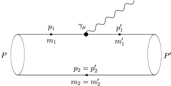
Figure 1: Feynman diagram corresponding to the quark in the ‘meson’ $A(B)$ emitting the photon for the transition $A(P)\to B(P^{\prime})+\gamma(Q)$.

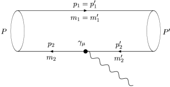
Figure 2: Feynman diagram corresponding to the anti-quark in the ‘meson’ $A(B)$ emitting the photon for the transition $A(P)\to B(P^{\prime})+\gamma(Q)$.

As an example of the radiative transitions, let us consider a decay $A(P)\to B(P^{\prime})+\gamma(Q)$, and we will take this example to show the formulation for the decays in terms of the BS wave functions and how the electromagnetic (an Abelien) gauge invariance is guaranteed throughout the paper. Here the ‘meson’ $A$ (a bound state) consists of a quark $q_{1}:p_{1},m_{1}$ and an anti-quark $\bar{q}_{2}:p_{2},m_{2}$, and the ‘meson’ $B$ (another bound state), similar to $A$, consists of a quark $q^{\prime}_{1}:p^{\prime}_{1},m^{\prime}_{1}$ and an anti-quark $\bar{q}^{\prime}_{2}:p^{\prime}_{2},m^{\prime}_{2}$. To be responsible for the decay, the Feynman diagrams for the lowest order are described as Fig.1 and Fig.2.

Since the concerned process is an electromagnetic transition, and if it is ‘automatic’ decay, the meson $A$ must be an excitation state of the meson $B$, i.e., we must have $m_{1}=m^{\prime}_{1},m_{2}=m^{\prime}_{2}$. For more specific, we further assume that in the mesons, the quarks $q_{1},q^{\prime}_{1}:(p_{1},m_{1}),(p^{\prime}_{1},m^{\prime}_{1})$, carry charge $Q_{1}$ in the unit $e$ and the anti-quarks $\bar{q}_{2},\bar{q}^{\prime}_{2}:(p_{2},m_{2}),(p^{\prime}_{2},m^{\prime}_{2})$, carry charge $Q_{2}$ in the unit $e$. In fact, in many discussions, proving the gauge invariance and the other derivations, the contributions from quark $q_{1}$ Fig.1 and those from anti-quark $\bar{q_{2}}$ Fig.2 are independent, thus to investigate the decay amplitude, either the quark emission of a photon Fig.1 or the anti-quark emission Fig.2 may be taken as ‘a representation’ of the transition (to consider one of them is enough, the other is almost the same just to repeat once more if one consider both of them for completeness, so here we say ‘a representation’). In Refs.mand ; compos , how to write down the S-matrix element for this kind of decays in terms of BS wave function is given:

$$<P^{\prime},Q\,\epsilon|S|P>=\frac{(2\pi)^{4}e}{\sqrt{2^{3}\omega\omega_{A}\omega_{B}}}\delta^{4}(P^{\prime}+Q-P)\epsilon^{\mu}\cdot<P^{\prime}|J_{\mu}|P>,$$

here $\epsilon^{\mu}$ is the polarization vector of the photon and the matrix element for the current (Figs.1,2):

$$<P^{\prime}|J_{\mu}|P>=\frac{1}{(2\pi)^{4}}\int d^{4}q^{\prime}\int d^{4}qTr\left\{\bar{\chi}_{P^{\prime}}(q^{\prime})\left[G^{(1)}_{\mu}(P^{\prime}q^{\prime};Q;P,q)+G^{(2)}_{\mu}(P^{\prime}q^{\prime};Q;P,q)\right]{\chi}_{P}(q)\right\}$$

$$=\frac{1}{(2\pi)^{4}}\int d^{4}q^{\prime}\int d^{4}qTr\left\{\bar{\chi}_{P^{\prime}}(q^{\prime})Q_{1}\gamma^{(1)}_{\mu}{\chi}_{P}(q)[S^{(2)}_{f}(q^{\prime}-\alpha^{\prime}_{2}P^{\prime})]^{-1}\cdot\delta^{4}(q-q^{\prime}+\alpha^{\prime}_{2}P^{\prime}-\alpha_{2}P)\right.$$

$$\left.+\bar{\chi}_{P^{\prime}}(q^{\prime})[S^{(1)}_{f}(\alpha_{1}P+q)]^{-1}{\chi}_{P}(q)Q_{2}\gamma^{(2)}_{\mu}\cdot\delta^{4}(q-q^{\prime}+\alpha_{1}P-\alpha^{\prime}_{1}P^{\prime})\right\}\,,$$ (8)

namely corresponding to the irreducible Feynman diagrams Figs.(1,2), the operators (factors) $G^{(i)}_{\mu}(P^{\prime}q^{\prime};Q;P,q),(i=1,2)$ are defined by

$$\bar{\chi}_{P^{\prime}}(q^{\prime})G^{(1)}_{\mu}(P^{\prime}q^{\prime};Q;P,q){\chi}_{P}(q)\equiv\bar{\chi}_{P^{\prime}}(q^{\prime})Q_{1}\gamma^{(1)}_{\mu}{\chi}_{P}(q)[S^{(2)}_{f}(q^{\prime}-\alpha^{\prime}_{2}P^{\prime})]^{-1}\delta(q-q^{\prime}+\alpha^{\prime}_{2}P^{\prime}-\alpha_{2}P)\,;$$

$$\bar{\chi}_{P^{\prime}}(q^{\prime})G^{(2)}_{\mu}(P^{\prime}q^{\prime};Q;P,q){\chi}_{P}(q)\equiv\bar{\chi}_{P^{\prime}}(q^{\prime})[S^{(1)}_{f}(\alpha_{1}P+q)]^{-1}{\chi}_{P}(q)Q_{2}\gamma^{(2)}_{\mu}\cdot\delta^{4}(q-q^{\prime}+\alpha_{1}P-\alpha^{\prime}_{1}P^{\prime})\,.$$

Here the quarks’ momenta, $p_{1},p^{\prime}_{1}$, and anti-quarks’ momenta, $p_{2},p^{\prime}_{2}$, are related to the total momenta $P,P^{\prime}$ and the relative ones $q,q^{\prime}$ of the initial meson $A$ and the finial meson $B$ respectively:

$$p_{1}={\alpha}_{1}P+q\,,\;\;{\alpha}_{1}\equiv\frac{m_{1}}{m_{1}+m_{2}}\,,\;\;\;p_{2}={\alpha}_{2}P-q,\;\;{\alpha}_{2}\equiv\frac{m_{2}}{m_{1}+m_{2}}\,;$$

$$p^{\prime}_{1}={\alpha}^{\prime}_{1}P^{\prime}+q^{\prime}\,,\;\;{\alpha}^{\prime}_{1}\equiv\frac{m^{\prime}_{1}}{m^{\prime}_{1}+m^{\prime}_{2}}\,,\;\;\;p^{\prime}_{2}={\alpha}^{\prime}_{2}P^{\prime}-q^{\prime}\,,\;\;{\alpha}^{\prime}_{2}\equiv\frac{m^{\prime}_{2}}{m^{\prime}_{1}+m^{\prime}_{2}}\,.$$ (9)

In Eq.(II.2) ‘$Tr$’ denotes the trace for the $\gamma$-matrices is taken. ${\chi}_{P}(q)$ and $\bar{\chi}_{P^{\prime}}(q^{\prime})$ are the relevant BS wave functions of the mesons $A$ and $B$; $S^{(i)}_{f}(i=1,2)$ are the propagator of the quark and anti-quark. $Q=P-P^{\prime}$ is the photon’s four momentum. Since the decay is electromagnetic, i.e., the flavor(s) is(are) conserved, so we have $m_{1}=m^{\prime}_{1}$ and $m_{2}=m^{\prime}_{2}$, that $\alpha_{1}=\alpha^{\prime}_{1},\alpha_{2}=\alpha^{\prime}_{2}$ and $\alpha^{\prime}_{i}P^{\prime}-\alpha_{i}P=-\alpha_{i}Q,(i=1,2)$. Thus later on we simplify Eq.(II.2) by taking $m_{1}=m^{\prime}_{1}$ and $m_{2}=m^{\prime}_{2}$ always.

In Refs.mand ; compos , the operators $G^{(1)}_{\mu}(P^{\prime}q^{\prime};Q;P,q)$ and $G^{(2)}_{\mu}(P^{\prime}q^{\prime};Q;P,q)$ are obtained by analyzing the Feynman diagrams and to be sure only the ‘irreducible’ diagrams are involved. In fact, the amplitude being gauge invariant also means the operators have very definite relation to the BS equation (the ‘differential operator $\overrightarrow{O}(P,q,q^{\prime})$ or $\overleftarrow{O}(P,q,q^{\prime})$’ and the kernel $V(P,q,q^{\prime})$). Let us show the relation of the operators to the BS equation in the following subsection.

II.3 The Electromagnetic Gauge Invariance of the Radiative Transitions

According to Refs.lee ; changh , when a transition current matrix element, in which there is(are) bound state(s) being involved, is formulated in terms of BS equation, such as Eq.(II.2), and if one requests it is gauge invariant (the current is conserved), then the transition operators $G^{(i)}_{\mu}(P^{\prime},q^{\prime};Q;P,q)(i=1,2)$, which appear in Eq.(II.2) and correspond to the irreducible Feynman diagrams, must ‘match’ with the BS equation accordingly in an exact way. Therefore, to determine a specific $G^{(i)}_{\mu}(P^{\prime},q^{\prime};Q;P,q)$ and to guarantee the matrix element being gauge invariant, we need to explore the match rule precisely.

Now let us ‘explore’ the match rule and show the specific $G^{(i)}_{\mu}(P^{\prime},q^{\prime};Q;P,q)$ happens to be satisfied with the match rule, when the BS wave functions adopted in Eq.(II.2) correspond to the solutions of the equation with the ‘lowest’ order kernel.

To explore the ‘match rule’, first of all, let us introduce an external classical field $A^{ex}_{\mu}$ and in the underlying theory add a coupling term:

$$J^{\mu}_{em}(x)A^{ex}_{\mu}(x),$$ (10)

to the Lagrangian, here $J^{\mu}_{em}$ is the electromagnetic current of the field theory. Then being parallel the case without the $A^{ex}_{\mu}$, one now may establish a BS equation with the external field $A^{ex}_{\mu}$ through the coupling term Eq.(10), and the BS equation operators $\overrightarrow{O^{A^{ex}_{\mu}}}$ and $\overrightarrow{V^{A^{ex}_{\mu}}}$ may be obtained accordingly. With the preparations, the ‘match rule’ can be stated as that $G_{\mu}$, the irreducible Feynman diagrams, should be exactly obtained as the the following way:

$$\{G_{\mu}\}\equiv\sum_{i=1,2}G^{(i)}_{\mu}(P^{\prime},q^{\prime};Q;P,q)=\frac{\delta(\overrightarrow{O^{A^{ex}_{\mu}}}-\overrightarrow{V^{A^{ex}_{\mu}}})}{\delta A^{ex}_{\mu}}\;|_{A^{ex}_{\mu}\rightarrow 0}\,.$$ (11)

The Eq.(11), in fact, can be explained as that the irreducible Feynman diagrams, $G_{\mu}$, should be obtained by the way that the photon line attaches onto each charged line in the BS equation operators $O(P,q^{\prime},q)-V(P,q^{\prime},q)$ once in turn. To be precise, let us take the example to explain Eq.(11) and its meaning.

With the match rule between $G_{\mu}(P^{\prime},q^{\prime};Q;P,q)$ and BS equation, let us turn back to examine the specific $G^{(i)}_{\mu}(P^{\prime},q^{\prime};Q;P,q)$ in Eq.(II.2). If the BS kernel $V(P,q^{\prime},q)$ for the bound states $P,P^{\prime}$ of quark and anti-quark is just one gluon exchange

$$\int d^{4}q^{\prime}\bar{\chi}_{P}(q^{\prime})V(P,q^{\prime},q)=\int d^{4}q^{\prime}\gamma_{\mu}^{(2)}\bar{\chi}_{P}(q^{\prime})\gamma_{\mu}^{(1)}D_{f}(q^{\prime}-q)$$

or

$$\int d^{4}qV(P,q^{\prime},q)\chi_{P}(q)=\int d^{4}q\gamma_{\mu}^{(1)}\chi_{P}(q)\gamma_{\mu}^{(2)}D_{f}(q^{\prime}-q)\,,$$ (12)

i.e. $D_{f}$ is the gluon propagator, and in the underlying theory the quark carries charge $Q_{1}$ in unit of $e$ and the anti-quark carries $Q_{2}$ that means in the electromagnetic current $J^{\mu}_{em}$ Eq.(10) there are quark current $Q_{1}J^{(1)}_{\mu}$ and anti-quark $Q_{2}J^{(2)}_{\mu}$, hence by Eq.(11) for the transition the irreducible Feynman diagrams $G^{(1)}_{\mu}(P^{\prime},q^{\prime};Q;P,q)$ is generated by attaching the photon line onto the quark line in $O(P,q^{\prime},q)-V(P,q^{\prime},q)$ (Fig.1a) and $G^{(2)}_{\mu}(P^{\prime},q^{\prime};Q;P,q)$ is generated by attaching the photon line onto the anti-quark line in $O(P,q^{\prime},q)-V(P,q^{\prime},q)$ (Fig.1b) as indicated in Eq.(II.2). Note here that since $V(P,q^{\prime},q)$ is neutral so according to the match rule there is no contribution from $V(P,q^{\prime},q)$ at all, thus the photon line can attach onto those lines in $O(P,q^{\prime},q)$ of the BS equation only.

Now following Refs.lee ; changh , let us show the gauge invariance, i.e. the current matrix element is conserved.

To apply the equations $Q=P-P^{\prime}$ and the general identity

$$-iQ^{\mu}\gamma^{(1)}_{\mu}=[S^{(1)}_{f}(\alpha_{1}P+q)]^{-1}-[S^{(1)}_{f}(\alpha^{\prime}_{1}P^{\prime}+q^{\prime})]^{-1}\,,$$

$$iQ^{\mu}\gamma^{(2)}_{\mu}=[S^{(2)}_{f}(-\alpha_{2}P+q)]^{-1}-[S_{f}^{(2)}(-\alpha^{\prime}_{2}P^{\prime}+q^{\prime})]^{-1}\,,$$ (13)

we have

$$-iQ^{\mu}<P^{\prime}|J_{\mu}|P>=\int d^{4}q^{\prime}\int d^{4}qTr\left\{\bar{\chi}_{P^{\prime}}(q^{\prime})Q_{1}\left([S_{f}^{(1)}(\alpha_{1}P+q)]^{-1}\right.\right.$$

$$\left.\left.-[S_{f}^{(1)}(\alpha^{\prime}_{1}P^{\prime}+q^{\prime})]^{-1}\right){\chi}_{P}(q)[S^{(2)}_{f}(-\alpha^{\prime}_{2}P^{\prime}+q^{\prime})]^{-1}\delta^{4}(q-q^{\prime}-\alpha_{2}Q)-\right.$$

$$\left.\bar{\chi}_{P^{\prime}}(q^{\prime})[S_{f}^{(1)}(\alpha_{1}P+q)]^{-1}{\chi}_{P}(q)Q_{2}\left([S^{(2)}_{f}(-\alpha_{2}P+q)]^{-1}-[S_{f}^{(2)}(-\alpha^{\prime}_{2}P^{\prime}+q^{\prime})]^{-1}\right)\delta^{4}(q-q^{\prime}+\alpha_{1}Q)\right\}$$

$$=\int d^{4}q^{\prime}\int d^{4}qTr\bar{\chi}_{P^{\prime}}(q^{\prime})\left\{Q_{1}\left[\overrightarrow{O}(P,q^{\prime}+\alpha_{2}Q,q)-\overleftarrow{O}(P^{\prime},q^{\prime},q-\alpha_{2}Q)\right]+Q_{2}\left[\cdots\right]\right\}{\chi}_{P}(q)\,.$$ (14)

Considering the property of the BS kernel $V$ indicated by Eq.(12)

$$\bar{\chi}_{P^{\prime}}(q^{\prime})\overrightarrow{V}(P,q^{\prime}+\alpha_{2}Q,q)\chi_{P}(q)=\bar{\chi}_{P^{\prime}}(q^{\prime})\overleftarrow{V}(P^{\prime},q^{\prime},q-\alpha_{2}Q)\chi_{P}(q)\,,$$

and

$$\bar{\chi}_{P^{\prime}}(q^{\prime})\overrightarrow{V}(P,q^{\prime}-\alpha_{1}Q,q)\chi_{P}(q)=\bar{\chi}_{P^{\prime}}(q^{\prime})\overleftarrow{V}(P^{\prime},q^{\prime},q+\alpha_{1}Q)\chi_{P}(q)\,,$$ (15)

then Eq.(II.3) can be rewritten

$$-iQ^{\mu}<P^{\prime}|J_{\mu}|P>=$$

$$\int d^{4}q^{\prime}\int d^{4}qTr\left\{Q_{1}\bar{\chi}_{P^{\prime}}(q^{\prime})\left[\overrightarrow{O}(P,q^{\prime}+\alpha_{2}Q,q)-\overrightarrow{V}(P,q^{\prime}+\alpha_{2}Q,q)\right]{\chi}_{P}(q)\right.$$

$$-\left.Q_{1}\bar{\chi}_{P^{\prime}}(q^{\prime})\left[\overleftarrow{O}(P^{\prime},q^{\prime},q-\alpha_{2}Q)-\overleftarrow{V}(P^{\prime},q^{\prime},q-\alpha_{2}Q)\right]{\chi}_{P}(q)\right.$$

$$\left.+Q_{2}\bar{\chi}_{P^{\prime}}(q^{\prime})\left[\overrightarrow{O}(P,q^{\prime}-\alpha_{1}Q,q)-\overrightarrow{V}(P,q^{\prime}-\alpha_{1}Q,q)\right]{\chi}_{P}(q)\right.$$

$$-\left.Q_{2}\bar{\chi}_{P^{\prime}}(q^{\prime})\left[\overleftarrow{O}(P^{\prime},q^{\prime},q+\alpha_{1}Q)-\overleftarrow{V}(P^{\prime},q^{\prime},q+\alpha_{1}Q)\right]{\chi}_{P}(q)\right\}\,.$$ (16)

It is easy to see when the BS equations Eq.(II.1) are applied to Eq.(II.3) for $\bar{\chi}_{P^{\prime}}(p)$ and $\chi_{P}(q)$ respectively, the matrix element of the current is conserved

$$-iQ^{\mu}<P^{\prime}|J_{\mu}|P>=0\,,$$ (17)

i.e. the Abel gauge invariance is proved.

Since the charge values $Q_{1}$ and $Q_{2}$ of the quark and anti-quark are independent, and one may also see from the above that the terms proportional to $Q_{1}$ and $Q_{2}$ are independent too, thus to prove the gauge invariance, it is enough to show one case, for instance, for the terms which are proportional to $Q_{1}$ only. Namely it is enough to show the terms proportional to $Q_{1}$ themselves are gauge invariance (for the terms which are proportional to $Q_{2}$ to show their gauge invariance is similar). Later on to shorten the presentation of the derivation, we only present those terms either proportional to $Q_{1}$ or to $Q_{2}$ precisely, and just add the statement as ‘the other terms are similar’ for instance.

III The Instantaneous Formulation for Radiative Transitions between Bound States and Its Gauge Invariance

Before deriving the instantaneous formulation for the transitions between bound states, first of all, we need to do some preparations, namely we need to re-write the ‘instantaneous’ BS equation in covariant formulation in a reference frame, in which the bound state may be moving.

III.1 The BS Equation with an Instantaneous Kernel and Its reduced Equation

The so-called ‘instantaneous approximation’ was realized by Salpeter first, and it is not Lorentz covariantsalp . In his original paper and in most literature, indeed an approximation was made in the rest frame of the concerned bound state. It says when the BS has an instantaneous kernel i.e. the kernel of BS does not depend on the time component of the relative momentum $k_{0}$, such as to take a simple form

$$V(P^{\mu},k^{\mu},q^{\mu})|_{\overrightarrow{P}=0}\simeq V(|\stackrel{{\scriptstyle\rightarrow}}{{k}}-\stackrel{{\scriptstyle\rightarrow}}{{q}}|)\,,$$ (18)

then as a main result of the ‘instantaneous approximation’, the four dimension BS equation can be reduced into a three-dimension Schrödinger equationsalp .

Whereas here when BS equation really has an instantaneous kernel, we reduce the BS equation without approximation in certain sense. Especially, we are considering the radiative transitions between the bound states, and we find that with an approximation as done by Salpeter the electromagnetic gauge invariance for the transitions cannot be guaranteed, thus we need to start the reducing of the BS equation with an instantaneous kernel from beginning, but to reduce the ‘instantaneous equation and the wave function’ in such a way that is the so-called instantaneous but Lorentz covariant.

To do so, first of all we divide the relative momentum $q$ into two components, $q_{{}_{\parallel}}$ and $q_{{}_{\perp}}$, a parallel component and an orthogonal one to the bound state momentum $P\;\;(P^{2}=M^{2})$ respectively:

$$q^{\mu}=q^{\mu}_{P_{\parallel}}+q^{\mu}_{P_{\perp}},$$

where $q^{\mu}_{P_{\parallel}}\equiv\frac{(P\cdot q)}{M^{2}}P^{\mu}$ and $q^{\mu}_{P_{\perp}}\equiv q^{\mu}-q^{\mu}_{P_{\parallel}}$. Correspondingly, we have two Lorentz invariant variables:

$$q_{P}=\frac{(P\cdot q)}{M}\,,\;\;\;\;q_{P_{T}}=\sqrt{q^{2}_{P}-q^{2}}=\sqrt{-q^{2}_{P_{\perp}}}\,.$$

In the rest frame of the concerned bound state, i.e., $\stackrel{{\scriptstyle\rightarrow}}{{P}}=0$, they turn to the usual components $q_{0}$ and $|\overrightarrow{q}|$, respectively. Now the integration element of the relative momentum $k$ can be written in an invariant form:

$$d^{4}k=dk_{P}k^{2}_{P_{T}}dk_{P_{T}}dsd\phi,$$ (19)

where $\phi$ is the azimuthal angle, $s=\frac{k_{P}q_{P}-(k\cdot q)}{k_{P_{T}}q_{P_{T}}}$. The interaction kernel Eq.(18) can be re-written as:

$$V(P^{\mu},k^{\mu},q^{\mu})=V(|k^{\mu}_{P_{\perp}}-q^{\mu}_{P_{\perp}}|).$$ (20)

Similar to Ref.salp , we introduce the ‘instantaneous’ BS wave function:

$$\varphi_{P}(q^{\mu}_{P_{\perp}})\equiv i\int\frac{dq_{P}}{2\pi}\chi_{P}(q^{\mu}_{P_{\parallel}},q^{\mu}_{P_{\perp}})\,,$$ (21)

and integration

$$\eta(q^{\mu}_{P_{\perp}})\equiv\int\frac{k^{2}_{P_{T}}dk_{P_{T}}ds}{(2\pi)^{2}}V(|k^{\mu}_{P_{\perp}}-q^{\mu}_{P_{\perp}}|)\varphi_{P}(k^{\mu}_{P_{\perp}})\,,$$ (22)

then the BS equation Eq.7 becomes

$$\chi_{P}(q^{\mu}_{P_{\parallel}},q^{\mu}_{P_{\perp}})=S_{f}^{(1)}(p^{\mu}_{1})\eta(q^{\mu}_{P_{\perp}})S_{f}^{(2)}(-p^{\mu}_{2}),$$ (23)

where $S_{f}^{(1)}(p_{1})$ and $S_{f}^{(2)}(-p_{2})$ are the propagators of the quark and anti-quark respectively. They can be decomposed as:

$$-iJS_{f}^{(i)}(Jp^{\mu}_{i})=\frac{\Lambda^{+}_{ip}(q^{\mu}_{P_{\perp}})}{Jq_{P}+\alpha_{i}M-\omega_{iP}+i\epsilon}+\frac{\Lambda^{-}_{ip}(q^{\mu}_{P_{\perp}})}{Jq_{P}+\alpha_{i}M+\omega_{iP}-i\epsilon}\,,$$ (24)

with

$$\omega_{iP}=\sqrt{m_{i}^{2}+q^{2}_{p_{T}}}\,,\;\;\;\;\Lambda^{\pm}_{iP}(q_{P_{\perp}})=\frac{1}{2\omega_{iP}}\left[\frac{\not\!\!{P}}{M}\omega_{iP}\pm J(m_{i}+{\not\!q}_{P_{\perp}})\right],$$ (25)

where $J=1$ for the quark($i=1$) and $J=-1$ for the anti-quark($i=2$). Here $\Lambda^{\pm}_{iP}(q_{P_{\perp}})$ satisfies the relations:

$$\Lambda^{+}_{iP}(q^{\mu}_{P_{\perp}})+\Lambda^{-}_{iP}(q^{\mu}_{P_{\perp}})=\frac{\not\!\!{P}}{M}\,,\;\;\Lambda^{\pm}_{iP}(q^{\mu}_{P_{\perp}})\frac{\not\!\!{P}}{M}\Lambda^{\pm}_{iP}(q^{\mu}_{P_{\perp}})=\Lambda^{\pm}_{iP}(q^{\mu}_{P_{\perp}})\,,\;\;\Lambda^{\pm}_{iP}(q^{\mu}_{P_{\perp}})\frac{\not\!\!{P}}{M}\Lambda^{\mp}_{iP}(q^{\mu}_{P_{\perp}})=0\,.$$ (26)

Namely $\Lambda^{\pm}$ may be considered as projection operators (the energy ($P$)-projection operators), while in the rest frame of the bound state, they turn to the energy projection operator.

For later discussions let us define $\varphi^{\pm\pm}_{P}(q^{\mu}_{P_{\perp}})$ as:

$$\varphi^{\pm\pm}_{P}(q^{\mu}_{P_{\perp}})\equiv\Lambda^{\pm}_{1P}(q^{\mu}_{P_{\perp}})\frac{\not\!\!{P}}{M}\varphi_{P}(q^{\mu}_{P_{\perp}})\frac{\not\!\!{P}}{M}\Lambda^{\pm}_{2P}(q^{\mu}_{P_{\perp}})\,,$$ (27)

then for the BS wave functions $\varphi_{P}(q^{\mu}_{P_{\perp}})$ we have:

$$\varphi_{P}(q^{\mu}_{P_{\perp}})=\varphi^{++}_{P}(q^{\mu}_{P_{\perp}})+\varphi^{+-}_{P}(q^{\mu}_{P_{\perp}})+\varphi^{-+}_{P}(q^{\mu}_{P_{\perp}})+\varphi^{--}_{P}(q^{\mu}_{P_{\perp}})\,.$$

Since the BS equation kernel is instantaneous, we may integrate out $q_{P}$ (contour integration) on both sides of Eq.(23), and obtain

$$\varphi_{P}(q^{\mu}_{P_{\perp}})=\frac{\Lambda^{+}_{1P}(q^{\mu}_{P_{\perp}})\eta_{P}(q^{\mu}_{P_{\perp}})\Lambda^{+}_{2P}(q^{\mu}_{P_{\perp}})}{(M-\omega_{1P}-\omega_{2P})}-\frac{\Lambda^{-}_{1P}(q^{\mu}_{P_{\perp}})\eta_{P}(q^{\mu}_{P_{\perp}})\Lambda^{-}_{2P}(q^{\mu}_{P_{\perp}})}{(M+\omega_{1P}+\omega_{2P})}\,,$$ (28)

and applying the energy ($P$)-projection operators $\Lambda^{\pm}_{iP}(q^{\mu}_{P_{\perp}})$ to Eq.(28) further, we obtain the coupled equations:

$$(M-\omega_{1P}-\omega_{2P})\varphi^{++}_{P}(q^{\mu}_{P_{\perp}})=\Lambda^{+}_{1P}(q^{\mu}_{P_{\perp}})\eta_{P}(q^{\mu}_{P_{\perp}})\Lambda^{+}_{2P}(q^{\mu}_{P_{\perp}})\,,$$ (29)

$$(M+\omega_{1P}+\omega_{2P})\varphi^{--}_{P}(q^{\mu}_{P_{\perp}})=-\Lambda^{-}_{1P}(q^{\mu}_{P_{\perp}})\eta_{P}(q^{\mu}_{P_{\perp}})\Lambda^{-}_{2P}(q^{\mu}_{P_{\perp}})\,,$$ (30)

$$\varphi^{+-}_{P}(q^{\mu}_{P_{\perp}})=\varphi^{-+}_{P}(q^{\mu}_{P_{\perp}})=0\,.$$ (31)

The normalization condition Eq.(5) now terns to the follows accordingly by the positive and negative functions as:

$$\int\frac{q_{T}^{2}dq_{T}}{(2\pi)^{2}}tr\left[\overline{\varphi}^{++}\frac{{/}\!\!\!{p}}{M}\varphi^{++}\frac{{/}\!\!\!{p}}{M}-\overline{\varphi}^{--}\frac{{/}\!\!\!{p}}{M}\varphi^{--}\frac{{/}\!\!\!{p}}{M}\right]=2P_{0}.$$ (32)

Note that Salpeter and many authors in literature considered that, of the above coupled equations Eqs.(29,30,31), the equation Eq.(29) is ‘dominant’, owing to having a very small coefficient $(M-\omega_{1P}-\omega_{2P})$ (weak binding) on the left hand side, and it is ‘projected’ by positive-positive energy project operators ($\Lambda^{+}_{1P}(q^{\mu}_{P_{\perp}})$ and $\Lambda^{+}_{2P}(q^{\mu}_{P_{\perp}})$) (it is why people call it as positive energy equation). Thus the authors highlighted on it only and dropped the rest equations out at all. With the approximation, they showed that if expending the equation Eq.(29) to the order of $\frac{q^{2}}{M^{2}}$ further, the equation may be turned into a Schrödinger one accordingly. Whereas, as emphasized in Introduction, we realized that if only keeping Eq.(29) and its solutions as wave functions to be applied to the radiative transitions, the gauge invariance will be violated. Thus here in the next two subsections we will show the formulation of the transitions between bound states in four dimension how to turns into an instantaneous one and accordingly how to keep the gauge invariance when the formulation in four dimension is gauge invariant precisely. It is just by considering all the coupled equations Eqs.(29,30,31) ‘equally’, and one will see that all of the equations play important roles in guaranteeing the gauge invariance for the radiative transitions between bound states.

To explore the contents of the Eqs.(29,30,31), here let us take a heavy quarkonium (or positronium) as samples to establish the coupled equations for the components in the instantaneous BS wave functions $\varphi_{P}(q^{\mu}_{P_{\perp}})$ and to show the equations are consistent.

Since a heavy quarkonium $(Q\bar{Q})$ is of equal masses ($m_{1}=m_{2}$, i.e., $\alpha_{1}=\alpha_{2}=\frac{1}{2}$), so its physical states have definite quantum number of $J^{PC}$, thus its equations should be given according to the quantum number precisely. Here we take the state with $J^{PC}=0^{-+}$ (total spin $S=0$, and total orbital angle moment $L=0$) as an example to show the main feature of the equations Eqs.(29,30,31). Of the components, the general relativistic wave function for the bound state with the quantum number $J^{PC}=0^{-+}$ (in the center of mass system) can be written as:

$$\varphi_{{}^{1}S_{0}}(\stackrel{{\scriptstyle\rightarrow}}{{q}})=\left[{\gamma_{0}}\varphi_{1}(\stackrel{{\scriptstyle\rightarrow}}{{q}})+\varphi_{2}(\stackrel{{\scriptstyle\rightarrow}}{{q}})+{\not\!q}_{\perp}\varphi_{3}(\stackrel{{\scriptstyle\rightarrow}}{{q}})+{\gamma_{0}}{\not\!q}_{\perp}\varphi_{4}(\stackrel{{\scriptstyle\rightarrow}}{{q}})\right]\gamma_{5}\,,$$ (33)

where ${q}_{\perp}=(0,\stackrel{{\scriptstyle\rightarrow}}{{q}})$. The equation Eq.(31), in fact it acts as constraints, give the strong conditions precisely:

$$\varphi_{1}(\stackrel{{\scriptstyle\rightarrow}}{{q}})=-m_{1}\varphi_{4}(\stackrel{{\scriptstyle\rightarrow}}{{q}}),\;\;\;\;\varphi_{3}(\stackrel{{\scriptstyle\rightarrow}}{{q}})=0\,.$$ (34)

Then we can rewrite the relativistic wave function of state $0^{-+}$ as:

$$\varphi_{{}^{1}S_{0}}(\stackrel{{\scriptstyle\rightarrow}}{{q}})=\left[{\gamma_{0}}\varphi_{1}(\stackrel{{\scriptstyle\rightarrow}}{{q}})+\varphi_{2}(\stackrel{{\scriptstyle\rightarrow}}{{q}})-{\gamma_{0}}{\not\!q}_{\perp}\frac{1}{m_{1}}\varphi_{1}(\stackrel{{\scriptstyle\rightarrow}}{{q}})\right]\gamma_{5}\,.$$ (35)

To apply the definition Eq.(27) to Eq.(35), the corresponding positive and negative projected wave functions may be written as:

$$\varphi^{++}_{{}^{1}S_{0}}(\stackrel{{\scriptstyle\rightarrow}}{{q}})=\frac{1}{2\omega_{1}m_{1}}\left(\omega_{1}\varphi_{1}(\stackrel{{\scriptstyle\rightarrow}}{{q}})+m_{1}\varphi_{2}(\stackrel{{\scriptstyle\rightarrow}}{{q}})\right)\left({\gamma_{0}}m_{1}+\omega_{1}-{\gamma_{0}}{\not\!q}_{\perp}\right)\gamma_{5}\,,$$ (36)

and

$$\varphi^{--}_{{}^{1}S_{0}}(\stackrel{{\scriptstyle\rightarrow}}{{q}})=\frac{1}{2\omega_{1}m_{1}}\left((\omega_{1}\varphi_{1}(\stackrel{{\scriptstyle\rightarrow}}{{q}})-m_{1}\varphi_{2}(\stackrel{{\scriptstyle\rightarrow}}{{q}})\right)\left({\gamma_{0}}m_{1}-\omega_{1}-{\gamma_{0}}{\not\!q}_{\perp}\right)\gamma_{5}\,.$$ (37)

From the reduced BS, Eqs.(29, 30) with a QCD inspired instantaneous kernel (relating to $V_{s}$ and $V_{v}$) for the $\eta$ in the equations and by taking different traces for the $\Gamma$ matrix, finally we obtain the couple equations for the components $\varphi_{1}({\stackrel{{\scriptstyle\rightarrow}}{{q}}})$ and $\varphi_{2}({\stackrel{{\scriptstyle\rightarrow}}{{q}}})$:

$$(M-2\omega_{1})\omega_{1}\left[\omega_{1}\varphi_{1}({\stackrel{{\scriptstyle\rightarrow}}{{q}}})+m_{1}\varphi_{2}({\stackrel{{\scriptstyle\rightarrow}}{{q}}})\right]$$

$$=-\int\frac{d{\stackrel{{\scriptstyle\rightarrow}}{{k}}}}{(2\pi)^{3}}\left[\left(m_{1}^{2}(V_{s}+2V_{v})-{\stackrel{{\scriptstyle\rightarrow}}{{q}}}\cdot{\stackrel{{\scriptstyle\rightarrow}}{{k}}}V_{s}\right)\varphi_{1}({\stackrel{{\scriptstyle\rightarrow}}{{k}}})+\omega_{1}m_{1}(V_{s}-4V_{v})\varphi_{2}({\stackrel{{\scriptstyle\rightarrow}}{{k}}})\right]\,,$$ (38)

$$(M+2\omega_{1})\omega_{1}\left[\omega_{1}\varphi_{1}({\stackrel{{\scriptstyle\rightarrow}}{{q}}})-m_{1}\varphi_{2}({\stackrel{{\scriptstyle\rightarrow}}{{q}}})\right]$$

$$=-\int\frac{d{\stackrel{{\scriptstyle\rightarrow}}{{k}}}}{(2\pi)^{3}}\left[\left(m_{1}^{2}(V_{s}+2V_{v})-{\stackrel{{\scriptstyle\rightarrow}}{{q}}}\cdot{\stackrel{{\scriptstyle\rightarrow}}{{k}}}V_{s}\right)\varphi_{1}({\stackrel{{\scriptstyle\rightarrow}}{{k}}})-\omega_{1}m_{1}(V_{s}-4V_{v})\varphi_{2}({\stackrel{{\scriptstyle\rightarrow}}{{k}}})\right]\,,$$ (39)

i.e. coupled equations for the eigenvalue $M$ and eigenfunctions, the wave functions $\varphi_{1}({\stackrel{{\scriptstyle\rightarrow}}{{q}}})$ and $\varphi_{2}({\stackrel{{\scriptstyle\rightarrow}}{{q}}})$. Note that we will derive and solve the equations with kernels $V_{s}$ (corresponding to scaler confinement) and $V_{v}$ (corresponding to one-gluon exchange) precisely elsewherechangwang , but here we only show the fact that when all of the equations Eqs.(29, 30, 31) are taken into account, consist coupled equations can be obtained finally without approximation.

By contrary, for Salpeter equation only the positive energy component equation Eq.(29) is kept, but further assumption on the spin structure (in four components) of the wave function $\varphi_{{}^{1}S_{0}}(\stackrel{{\scriptstyle\rightarrow}}{{q}})$ is madesalp , that is different from here, as shown, the spin structure is determined by the equations Eqs.(29, 30, 31) simultaneously.

In fact, the above coupled equations are written in the reference frame of the bound state itself. Whereas, to give the ‘instantaneous’ formulation for the transitions between the bound states, we also need to have the precise formulation for the BS equation (with ‘instantaneous’ kernel) in a reference frame of another bound state. It is similar to do as the above, so the precise formulation is put into Appendix A.

III.2 The Reduced Formulation for Radiative Transitions between the Bound States with Instantaneous Kernel

The transition matrix element for a process of a bound state emitting a photon can be written by the BS wave function as:

$$<P^{\prime}|J_{\mu}|P>=<P^{\prime}|J_{\mu}|P>_{1}+<P^{\prime}|J_{\mu}|P>_{2}\,,$$ (40)

where

$$<P^{\prime}|J_{\mu}|P>_{1} = \int\frac{d^{4}qd^{4}q^{\prime}}{(2\pi)^{4}}Tr\left\{\bar{\chi}_{P^{\prime}}Q_{1}\gamma_{\mu}{\chi}_{P}S^{-1}_{2}(-p_{2})\delta^{4}(p_{2}-p^{\prime}_{2})\right\}\,,$$

$$<P^{\prime}|J_{\mu}|P>_{2} = \int\frac{d^{4}qd^{4}q^{\prime}}{(2\pi)^{4}}Tr\left\{\bar{\chi}_{P^{\prime}}S^{-1}_{1}(p_{1}){\chi}_{P}Q_{2}\gamma_{\mu}\delta^{4}(p_{1}-p^{\prime}_{1})\right\}\,,$$ (41)

here we have used subscript $`1^{\prime}$ to denote the photon emitted only by the quark and $`2^{\prime}$ to denote the photon emitted by the anti-quark. In fact, when we consider the gauge invariance of the process, these two parts are independent and each one can be treated independently. So below when we show how to keep gauge invariance, we pay more efforts on the first one, and just to say similarly on the second one for shortening.

We have made instantaneous approach to the BS wave function and BS equation, furthermore in this subsection we do similar ‘job’ for the transition matrix elements.

As for the matrix element

$$\displaystyle<P^{\prime}|J_{\mu}|P>_{1}=Q_{1}\int\frac{d^{4}qd^{4}q^{\prime}}{(2\pi)^{4}}Tr\left\{S^{\prime}_{2}(-p^{\prime}_{2})\bar{\eta^{\prime}}_{P^{\prime}}S^{\prime}_{1}(p^{\prime}_{1})\gamma_{\mu}S_{1}(p_{1}){\eta}_{P}S_{2}(-p_{2})S^{-1}_{2}(-p_{2})\delta^{4}(p_{2}-p^{\prime}_{2})\right\}$$

$$\displaystyle=Q_{1}\int\frac{d^{4}qd^{4}q^{\prime}}{(2\pi)^{4}}Tr\left\{\bar{\eta^{\prime}}_{P^{\prime}}S^{\prime}_{1}(p^{\prime}_{1})\gamma_{\mu}S_{1}(p_{1}){\eta}_{P}S_{2}(-p_{2})\delta^{4}(p_{2}-p^{\prime}_{2})\right\}\,,$$

here the integral element $d^{4}q=d^{3}q_{{}_{P}{\perp}}dq_{P}$ and the $\delta$-function can be re-written by the relation:

$$\displaystyle\delta^{4}(p_{2}-p^{\prime}_{2})=-\delta^{3}({p_{2}}_{P\perp}-{p^{\prime}_{2}}_{P\perp})\times\frac{1}{2\pi i}\Bigl{(}\frac{1}{\alpha_{2}P_{P}-q_{P}-\alpha^{\prime}_{2}{P^{\prime}}_{P}+q^{\prime}_{P}+i\epsilon}$$

$$\displaystyle-\frac{1}{\alpha_{2}P_{P}-q_{P}-\alpha^{\prime}_{2}{P^{\prime}}_{P}+q^{\prime}_{P}-i\epsilon}\Bigr{)},$$ (42)

then with Eqs.(24, 25), the matrix element turns into

$$<P^{\prime}|J_{\mu}|P>_{1}=-Q_{1}\int\frac{d^{4}qd^{4}q^{\prime}}{(2\pi)^{4}}Tr\Bigl{\{}\bar{\eta^{\prime}}_{P^{\prime}}S^{\prime}_{1}(p^{\prime}_{1})\gamma_{\mu}S_{1}(p_{1}){\eta}_{P}S_{2}(-p_{2})\delta^{3}({p_{2}}_{P\perp}-{p^{\prime}_{2}}_{P\perp})$$

$$\times\frac{1}{2\pi i}(\frac{1}{\alpha_{2}P_{P}-q_{P}-\alpha^{\prime}_{2}{P^{\prime}}_{P}+q^{\prime}_{P}+i\epsilon}-\frac{1}{\alpha_{2}P_{P}-q_{P}-\alpha^{\prime}_{2}{P^{\prime}}_{P}+q^{\prime}_{P}-i\epsilon})\Bigr{\}}$$

$$=-Q_{1}\int\frac{d^{4}qd^{4}q^{\prime}}{(2\pi)^{4}}Tr\left\{\bar{\eta^{\prime}}_{P^{\prime}}S^{\prime}_{1}(p^{\prime}_{1})\gamma_{\mu}\left(\frac{\Lambda^{+}_{1}}{q_{P}+\alpha_{1}M-\omega_{1}+i\epsilon}+\frac{\Lambda^{-}_{1}}{q_{P}+\alpha_{1}M+\omega_{1}-i\epsilon}\right)\right.$$

$$\left.\times{\eta}_{P}\left(\frac{\Lambda^{+}_{2}}{-q_{P}+\alpha_{2}M-\omega_{2}+i\epsilon}+\frac{\Lambda^{-}_{2}}{-q_{P}+\alpha_{2}M+\omega_{2}-i\epsilon}\right)\delta^{3}({p_{2}}_{P\perp}-{p^{\prime}_{2}}_{P\perp})\right.$$

$$\left.\times\frac{1}{2\pi{i}}\left(\frac{1}{\alpha_{2}M-q_{P}-\alpha^{\prime}_{2}E^{\prime}+q^{\prime}_{P}+i\epsilon}-\frac{1}{\alpha_{2}M-q_{P}-\alpha^{\prime}_{2}E^{\prime}+q^{\prime}_{P}-i\epsilon}\right)\right\}\,.$$

To integrate over $q_{P}$ and in terms of Eqs.(29, 30) for the initial bound state, the above matrix element becomes the follows

$$<P^{\prime}|J_{\mu}|P>_{1}=-Q_{1}\int\frac{d^{3}q_{P\perp}d^{4}q^{\prime}}{(2\pi)^{4}}\delta^{3}({p_{2}}_{P\perp}-{p^{\prime}_{2}}_{P\perp})Tr\left\{\bar{\eta^{\prime}}_{P^{\prime}}S^{\prime}_{1}(p^{\prime}_{1})\gamma_{\mu}\left(-\frac{\varphi^{++}_{P}(q_{P\perp})}{M-\alpha_{2}E^{\prime}-\omega_{1}+q^{\prime}_{P}+i\epsilon}\right.\right.$$

$$\left.\left.+\frac{\varphi^{++}_{P}(q_{P\perp})}{-\alpha_{2}E^{\prime}+\omega_{2}+q^{\prime}_{P}-i\epsilon}-\frac{\Lambda^{+}_{1}{\eta}_{P}\Lambda^{-}_{2}}{(M-\omega_{1}+q^{\prime}_{P}-\alpha_{2}E^{\prime}+i\epsilon)(\alpha_{2}E^{\prime}+\omega_{2}-q^{\prime}_{P}-i\epsilon)}\right.\right.$$

$$\left.\left.-\frac{\Lambda^{-}_{1}{\eta}_{P}\Lambda^{+}_{2}}{(M+\omega_{1}+q^{\prime}_{P}-\alpha_{2}E^{\prime}-i\epsilon)(\alpha_{2}E^{\prime}-\omega_{2}-q^{\prime}_{P}+i\epsilon)}-\frac{\varphi^{--}_{P}(q_{P\perp})}{-\alpha_{2}E^{\prime}-\omega_{2}+q^{\prime}_{P}+i\epsilon}\right.\right.$$

$$\left.\left.+\frac{\varphi^{--}_{P}(q_{P\perp})}{M-\alpha_{2}E^{\prime}+\omega_{1}+q^{\prime}_{P}-i\epsilon}\right)\right\}\,.$$

To apply the formulae in appendix A and to carry out the the cantor integration over $q^{\prime}_{P}$, we have

$$<P^{\prime}|J_{\mu}|P>_{1}=Q_{1}\int\frac{d^{3}q_{P\perp}d^{3}q^{\prime}_{P\perp}}{(2\pi)^{3}}\delta^{3}({p_{2}}_{P\perp}-{p^{\prime}_{2}}_{P\perp})Tr\left\{\left(\frac{\bar{\eta^{\prime}}_{P^{\prime}}\Lambda^{\prime+}_{1{P^{\prime}}}(q^{\prime}_{P\perp})\gamma_{\mu}\varphi^{++}_{P}(q_{P\perp})}{E^{\prime}-\omega^{\prime}_{1}-\omega_{2}}\right.\right.$$

$$\left.\left.-\frac{\bar{\eta^{\prime}}_{P^{\prime}}\Lambda^{\prime-}_{1{P^{\prime}}}(q^{\prime}_{P\perp})\gamma_{\mu}\varphi^{++}_{P}(q_{P\perp})}{M-\omega_{1}-\omega^{\prime}_{1}-E^{\prime}}-\frac{\bar{\eta^{\prime}}_{P^{\prime}}\Lambda^{\prime-}_{1{P^{\prime}}}(q^{\prime}_{P\perp})\gamma_{\mu}\Lambda^{+}_{1}{\eta}_{P}\Lambda^{-}_{2}}{(M-\omega_{1}-\omega^{\prime}-E^{\prime})(E^{\prime}+\omega^{\prime}_{1}+\omega_{2})}\right.\right.$$

$$\left.\left.+\frac{\bar{\eta^{\prime}}_{P^{\prime}}\Lambda^{\prime+}_{1{P^{\prime}}}(q^{\prime}_{P\perp})\gamma_{\mu}\Lambda^{-}_{1}{\eta}_{P}\Lambda^{+}_{2}}{(M+\omega_{1}+\omega^{\prime}-E^{\prime})(E^{\prime}-\omega^{\prime}_{1}-\omega_{2})}-\frac{\bar{\eta^{\prime}}_{P^{\prime}}\Lambda^{\prime+}_{1{P^{\prime}}}(q^{\prime}_{P\perp})\gamma_{\mu}\varphi^{--}_{P}(q_{P\perp})}{M+\omega_{1}+\omega^{\prime}_{1}-E^{\prime}}\right.\right.$$

$$\left.\left.+\frac{\bar{\eta^{\prime}}_{P^{\prime}}\Lambda^{\prime-}_{1{P^{\prime}}}(q^{\prime}_{P\perp})\gamma_{\mu}\varphi^{--}_{P}(q_{P\perp})}{E^{\prime}+\omega^{\prime}_{1}+\omega_{2}}\right)\right\}\,.$$

Here we have $\delta^{3}({p_{2}}_{P\perp}-{p^{\prime}_{2}}_{P\perp})$, $\omega^{\prime}_{2}=\omega_{2}$, $\Lambda^{\prime\pm}_{2{P^{\prime}}}(q^{\prime}_{P\perp})=\Lambda^{\pm}_{2{P}}(q_{P\perp})$, the identity $1\equiv\frac{\not\!{P}}{M}\frac{\not\!{P}}{M}=\frac{\not\!{P}}{M}\left(\Lambda^{{\prime}+}_{2}+\Lambda^{{\prime}-}_{2}\right)$ and the equations Eqs.(29, 30) for the final bound state, to apply all of them to the matrix element, we finally obtain:

$$\displaystyle<P^{\prime}|J_{\mu}|P>_{1}=Q_{1}\int\frac{d^{3}q_{P\perp}d^{3}q^{\prime}_{P\perp}}{(2\pi)^{3}}\delta^{3}({p_{2}}_{P\perp}-{p^{\prime}_{2}}_{P\perp})Tr\left\{\frac{\not\!{P}}{M}\left[\bar{\varphi^{\prime}}^{++}_{P^{\prime}}\gamma_{\mu}{\varphi}^{++}_{P}+\frac{\bar{\varphi^{\prime}}^{++}_{P^{\prime}}\gamma_{\mu}\Lambda^{-}_{1}{\eta}_{P}\Lambda^{+}_{2}}{M+\omega_{1}+\omega^{\prime}_{1}-E^{\prime}}\right.\right.$$

$$\displaystyle\left.\left.-\frac{\Lambda^{\prime-}_{2{P^{\prime}}}(q^{\prime}_{P\perp})\bar{\eta^{\prime}}_{P^{\prime}}\Lambda^{\prime+}_{1{P^{\prime}}}(q^{\prime}_{P\perp})\gamma_{\mu}\varphi^{--}_{P}(q_{P\perp})}{M+\omega_{1}+\omega^{\prime}_{1}-E^{\prime}}-\frac{\Lambda^{\prime+}_{2{P^{\prime}}}(q^{\prime}_{P\perp})\bar{\eta^{\prime}}_{P^{\prime}}\Lambda^{\prime-}_{1{P^{\prime}}}(q^{\prime}_{P\perp})\gamma_{\mu}\varphi^{++}_{P}(q_{P\perp})}{M-\omega_{1}-\omega^{\prime}_{1}-E^{\prime}}\right.\right.$$

$$\displaystyle\left.\left.+\frac{\bar{\varphi^{\prime}}^{--}_{P^{\prime}}\gamma_{\mu}\Lambda^{+}_{1}{\eta}_{P}\Lambda^{-}_{2}}{M-\omega_{1}-\omega^{\prime}_{1}-E^{\prime}}-\bar{\varphi^{\prime}}^{--}_{P^{\prime}}\gamma_{\mu}{\varphi}^{--}_{P}\right]\right\}\,.$$ (43)

If we define:

$${\psi}_{1P}^{-+}\equiv\frac{\Lambda^{-}_{1}(q_{P\perp}){\eta}_{P}\Lambda^{+}_{2}(q_{P\perp})}{M+\omega_{1}+\omega^{\prime}_{1}-E^{\prime}}\,,$$ (44)

$$\bar{\psi}_{1P^{\prime}}^{\prime-+}\equiv\frac{\Lambda^{\prime-}_{2{P^{\prime}}}(q^{\prime}_{P\perp})\bar{\eta}^{\prime}_{P^{\prime}}\Lambda^{\prime+}_{1{P^{\prime}}}(q^{\prime}_{P\perp})}{M+\omega_{1}+\omega^{\prime}_{1}-E^{\prime}}\,,$$ (45)

$$\bar{\psi}_{1P^{\prime}}^{\prime+-}\equiv\frac{\Lambda^{\prime+}_{2{P^{\prime}}}(q^{\prime}_{P\perp})\bar{\eta^{\prime}}_{P^{\prime}}\Lambda^{\prime-}_{1{P^{\prime}}}(q^{\prime}_{P\perp})}{M-\omega_{1}-\omega^{\prime}_{1}-E^{\prime}}\,,$$ (46)

$${\psi}_{1P}^{+-}\equiv\frac{\Lambda^{+}_{1}(q_{P\perp}){\eta}_{P}\Lambda^{-}_{2}(q_{P\perp})}{M-\omega_{1}-\omega^{\prime}_{1}-E^{\prime}}\,,$$ (47)

the amplitude becomes

$$\displaystyle<P^{\prime}|J_{\mu}|P>_{1}=Q_{1}\int\frac{d^{3}q_{P\perp}d^{3}q^{\prime}_{P\perp}}{(2\pi)^{3}}\delta^{3}(-{q}_{P\perp}-\alpha_{2}{P^{\prime}}_{P\perp}+{q^{\prime}}_{P\perp})Tr\left\{\frac{\not\!{P}}{M}\left[\bar{\varphi^{\prime}}^{++}_{P^{\prime}}({q^{\prime}}_{P\perp})\gamma_{\mu}{\varphi}^{++}_{P}({q}_{P\perp})\right.\right.$$

$$\displaystyle\left.\left.+\bar{\varphi^{\prime}}^{++}_{P^{\prime}}({q^{\prime}}_{P\perp})\gamma_{\mu}{\psi}^{-+}_{P}({q}_{P\perp})-\bar{\psi^{\prime}}^{-+}_{P^{\prime}}({q^{\prime}}_{P\perp})\gamma_{\mu}{\varphi}^{--}_{P}({q}_{P\perp})-\bar{\psi^{\prime}}^{+-}_{P^{\prime}}({q^{\prime}}_{P\perp})\gamma_{\mu}{\varphi}^{++}_{P}({q}_{P\perp})\right.\right.$$

$$\left.\left.+\bar{\varphi^{\prime}}^{--}_{P^{\prime}}({q^{\prime}}_{P\perp})\gamma_{\mu}{\psi}^{+-}_{P}({q}_{P\perp})-\bar{\varphi^{\prime}}^{--}_{P^{\prime}}({q^{\prime}}_{P\perp})\gamma_{\mu}{\varphi}^{--}_{P}({q}_{P\perp})\right]\right\}\,.$$ (48)

To integrate over three dimensional $q^{\prime}_{P\perp}$ further, then we obtain the instantaneous transition matrix element $<P^{\prime}|J_{\mu}|P>_{1}$ in three dimensional formulation. To do the same derivation for $<P^{\prime}|J_{\mu}|P>_{2}$, the whole instantaneous transition matrix element becomes

$$<P^{\prime}|J_{\mu}|P>=<P^{\prime}|J_{\mu}|P>_{1}+<P^{\prime}|J_{\mu}|P>_{2}$$

$$\displaystyle=\int\frac{d^{3}q_{P\perp}}{(2\pi)^{3}}Tr\left\{Q_{1}\frac{\not\!{P}}{M}\left[\bar{\varphi^{\prime}}^{++}_{P^{\prime}}({q}_{P\perp}+\alpha_{2}{P^{\prime}}_{P\perp})\gamma_{\mu}{\varphi}^{++}_{P}({q}_{P\perp})+\bar{\varphi^{\prime}}^{++}_{P^{\prime}}({q}_{P\perp}+\alpha_{2}{P^{\prime}}_{P\perp})\gamma_{\mu}{\psi}^{-+}_{1P}({q}_{P\perp})\right.\right.$$

$$-\left.\left.\bar{\psi^{\prime}}^{-+}_{1P^{\prime}}({q}_{P\perp}+\alpha_{2}{P^{\prime}}_{P\perp})\gamma_{\mu}{\varphi}^{--}_{P}({q}_{P\perp})-\bar{\psi^{\prime}}^{+-}_{1P^{\prime}}({q}_{P\perp}+\alpha_{2}{P^{\prime}}_{P\perp})\gamma_{\mu}{\varphi}^{++}_{P}({q}_{P\perp})\right.\right.$$

$$+\left.\left.\bar{\varphi^{\prime}}^{--}_{P^{\prime}}({q}_{P\perp}+\alpha_{2}{P^{\prime}}_{P\perp})\gamma_{\mu}{\psi}^{+-}_{1P}({q}_{P\perp})-\bar{\varphi^{\prime}}^{--}_{P^{\prime}}({q}_{P\perp}+\alpha_{2}{P^{\prime}}_{P\perp})\gamma_{\mu}{\varphi}^{--}_{P}({q}_{P\perp})\right]\right.$$

$$+\left.Q_{2}\left[\bar{\varphi^{\prime}}^{++}_{P^{\prime}}({q}_{P\perp}-\alpha_{1}{P^{\prime}}_{P\perp})\frac{\not\!{P}}{M}{\varphi}^{++}_{P}({q}_{P\perp})+\bar{\varphi^{\prime}}^{++}_{P^{\prime}}({q}_{P\perp}-\alpha_{1}{P^{\prime}}_{P\perp})\frac{\not\!{P}}{M}{\psi}^{+-}_{2P}({q}_{P\perp})\right.\right.$$

$$-\left.\left.\bar{\psi^{\prime}}^{+-}_{2P^{\prime}}({q}_{P\perp}-\alpha_{1}{P^{\prime}}_{P\perp})\frac{\not\!{P}}{M}{\varphi}^{--}_{P}({q}_{P\perp})-\bar{\psi^{\prime}}^{-+}_{2P^{\prime}}({q}_{P\perp}-\alpha_{1}{P^{\prime}}_{P\perp})\frac{\not\!{P}}{M}{\varphi}^{++}_{P}({q}_{P\perp})\right.\right.$$

$$+\left.\left.\bar{\varphi^{\prime}}^{--}_{P^{\prime}}({q}_{P\perp}-\alpha_{1}{P^{\prime}}_{P\perp})\frac{\not\!{P}}{M}{\psi}^{-+}_{2P}({q}_{P\perp})-\bar{\varphi^{\prime}}^{--}_{P^{\prime}}({q}_{P\perp}-\alpha_{1}{P^{\prime}}_{P\perp})\frac{\not\!{P}}{M}{\varphi}^{--}_{P}({q}_{P\perp})\right]\gamma_{\mu}\right\}\,.$$ (49)

Here similar to the Eqs.(44-47), we have defined $\psi_{2P}^{\pm\mp}$ and ${\bar{\psi}}_{2P^{\prime}}^{\prime\pm\mp}$ as follows:

$${\psi}_{2P}^{+-}=\frac{\Lambda^{+}_{1}(q_{P\perp}){\eta}_{P}\Lambda^{-}_{2}(q_{P\perp})}{M+\omega_{2}+\omega^{\prime}_{2}-E^{\prime}}\,,$$ (50)

$$\bar{\psi}_{2P^{\prime}}^{\prime+-}=\frac{\Lambda^{\prime+}_{2{P^{\prime}}}(q^{\prime}_{P\perp})\bar{\eta}^{\prime}_{P^{\prime}}\Lambda^{\prime-}_{1{P^{\prime}}}(q^{\prime}_{P\perp})}{M+\omega_{2}+\omega^{\prime}_{2}-E^{\prime}}\,,$$ (51)

$$\bar{\psi}_{2P^{\prime}}^{\prime-+}=\frac{\Lambda^{\prime-}_{2{P^{\prime}}}(q^{\prime}_{P\perp})\bar{\eta^{\prime}}_{P^{\prime}}\Lambda^{\prime+}_{1{P^{\prime}}}(q^{\prime}_{P\perp})}{M-\omega_{2}-\omega^{\prime}_{2}-E^{\prime}}\,,$$ (52)

$${\psi}_{2P}^{-+}=\frac{\Lambda^{-}_{1}(q_{P\perp}){\eta}_{P}\Lambda^{+}_{2}(q_{P\perp})}{M-\omega_{2}-\omega^{\prime}_{2}-E^{\prime}}\,.$$ (53)

If one takes the approximation ${\varphi}^{--}_{P}({q}_{P\perp})\simeq 0$, the matrix element becomes

$$<P^{\prime}|J_{\mu}|P>=<P^{\prime}|J_{\mu}|P>_{1}+<P^{\prime}|J_{\mu}|P>_{2}$$

$$\displaystyle=\int\frac{d^{3}q_{P\perp}}{(2\pi)^{3}}Tr\left\{Q_{1}\frac{\not\!{P}}{M}\left[\bar{\varphi^{\prime}}^{++}_{P^{\prime}}({q}_{P\perp}+\alpha_{2}{P^{\prime}}_{P\perp})\gamma_{\mu}{\varphi}^{++}_{P}({q}_{P\perp})\right.\right.$$

$$\displaystyle+\left.\left.\bar{\varphi^{\prime}}^{++}_{P^{\prime}}({q}_{P\perp}+\alpha_{2}{P^{\prime}}_{P\perp})\gamma_{\mu}{\psi}^{-+}_{1P}({q}_{P\perp})-\bar{\psi^{\prime}}^{+-}_{1P^{\prime}}({q}_{P\perp}+\alpha_{2}{P^{\prime}}_{P\perp})\gamma_{\mu}{\varphi}^{++}_{P}({q}_{P\perp})\right]\right.$$

$$\displaystyle+\left.Q_{2}\left[\bar{\varphi^{\prime}}^{++}_{P^{\prime}}({q}_{P\perp}-\alpha_{1}{P^{\prime}}_{P\perp})\frac{\not\!{P}}{M}{\varphi}^{++}_{P}({q}_{P\perp})+\bar{\varphi^{\prime}}^{++}_{P^{\prime}}({q}_{P\perp}-\alpha_{1}{P^{\prime}}_{P\perp})\frac{\not\!{P}}{M}{\psi}^{+-}_{2P}({q}_{P\perp})\right.\right.$$

$$\displaystyle-\left.\left.\bar{\psi^{\prime}}^{-+}_{2P^{\prime}}({q}_{P\perp}-\alpha_{1}{P^{\prime}}_{P\perp})\frac{\not\!{P}}{M}{\varphi}^{++}_{P}({q}_{P\perp})\right]\gamma_{\mu}\right\}\,.$$ (54)

Note that even when the approximation ${\varphi}^{--}_{P}({q}_{P\perp})\simeq 0$ is made, from Eq.(54) one may see that it is still not correct to calculate the matrix element by means of

$$<P^{\prime}|J_{\mu}|P>=<P^{\prime}|J_{\mu}|P>_{1}+<P^{\prime}|J_{\mu}|P>_{2}$$

$$\displaystyle=\int\frac{d^{3}q_{P\perp}}{(2\pi)^{3}}Tr\left\{Q_{1}\frac{\not\!{P}}{M}\left[\bar{\varphi^{\prime}}^{++}_{P^{\prime}}({q}_{P\perp}+\alpha_{2}{P^{\prime}}_{P\perp})\gamma_{\mu}{\varphi}^{++}_{P}({q}_{P\perp})\right]\right.$$

$$\displaystyle+\left.Q_{2}\left[\bar{\varphi^{\prime}}^{++}_{P^{\prime}}({q}_{P\perp}-\alpha_{1}{P^{\prime}}_{P\perp})\frac{\not\!{P}}{M}{\varphi}^{++}_{P}({q}_{P\perp})\right]\gamma_{\mu}\right\}\,.$$ (55)

III.3 The Gauge Invariance of Instantaneous Transition Matrix Element

In Sec.II, we showed that the transition matrix element is gauge invariant no matter the instantaneous approach is applied to, i.e.,

$$\displaystyle-iQ^{\mu}<P^{\prime}|J_{\mu}|P>_{1}=\frac{1}{(2\pi)^{4}}\int d^{4}q^{\prime}\int d^{4}qTr\left\{\bar{\chi}_{P^{\prime}}(q^{\prime})Q_{1}\left([S_{f}^{(1)}(\alpha_{1}P+q)]^{-1}\right.\right.$$

$$\left.\left.-[S_{f}^{(1)}(\alpha^{\prime}_{1}P^{\prime}+q^{\prime})]^{-1}\right){\chi}_{P}(q)[S^{(2)}_{f}(-\alpha^{\prime}_{2}P^{\prime}+q^{\prime})]^{-1}\delta^{4}(q-q^{\prime}-\alpha_{2}Q)\right\}=0\,.$$ (56)

In this subsection, we show that the instantaneous transition matrix element Eq.(49) is also gauge invariant, in terms of the gauge invariance in four dimensional formulation Eq.(56 and the instantaneous equations Eqs.(29,30,31).

First of all, let us examine how the equation Eq.(56) turns to a three dimensional one when the kernel of the considered BS equation is instantaneous. To substitute the BS wave functions $\chi_{P}(q)$ and $\bar{\chi}_{P^{\prime}}(q^{\prime})$ with BS equation Eq.(23), and similar to the above subsections, to deal with $\delta$ functions and then to integrate out $q_{P}$ and $q^{\prime}_{P}$ in the equation by contour integral, one immediately obtain

$$\displaystyle-iQ^{\mu}<P^{\prime}|J_{\mu}|P>_{1}=\int\frac{d^{4}qd^{4}q^{\prime}}{(2\pi)^{4}}Tr\left\{S_{f}^{{}^{\prime}(2)}(-p^{\prime}_{2})\bar{\eta}_{P^{\prime}}S_{f}^{{}^{\prime}(1)}(p^{\prime}_{1}){\eta}_{P}-\bar{\eta}_{P^{\prime}}S_{f}^{(1)}(p_{1}){\eta}_{P}S_{f}^{(2)}(-p_{2})\right\}$$

$$\displaystyle\times\delta^{3}({p_{2}}_{P\perp}-{p^{\prime}_{2}}_{P\perp})\delta(\alpha_{2}M-q_{P}-\alpha_{2}{P^{\prime}}_{P}+q^{\prime}_{P})$$

$$\displaystyle=-{2\pi i}\int\frac{d^{3}q_{\perp}d^{3}q^{\prime}_{\perp}\delta^{3}({p_{2}}_{\perp}-{p^{\prime}_{2}}_{\perp})}{(2\pi)^{4}}Tr\left\{\bar{\varphi}^{\prime++}_{P^{\prime}}{\eta}_{P}-\bar{\varphi}^{\prime--}_{P^{\prime}}{\eta}_{P}-\bar{\eta}_{P^{\prime}}{\varphi}^{++}_{P_{i}}+\bar{\eta}_{P^{\prime}}{\varphi}^{--}_{P}\right\}\,.$$ (57)

Note here that with Eqs.(29, 30), we have the part in $Tr$ of Eq.(III.3):

$$\displaystyle\left\{\bar{\varphi}^{\prime++}_{P^{\prime}}{\eta}_{P}-\bar{\varphi}^{\prime--}_{P^{\prime}}{\eta}_{P}-\bar{\eta}_{P^{\prime}}{\varphi}^{++}_{P_{i}}+\bar{\eta}_{P^{\prime}}{\varphi}^{--}_{P}\right\}$$

$$\displaystyle=\left\{\frac{\Lambda^{\prime+}_{2{P^{\prime}}}(q^{\prime}_{P\perp})\bar{\eta^{\prime}}_{P^{\prime}}\Lambda^{\prime+}_{1{P^{\prime}}}(q^{\prime}_{P\perp})}{E^{\prime}-\omega_{2}-\omega^{\prime}_{1}}{\eta}_{P}+\frac{\Lambda^{\prime-}_{2{P^{\prime}}}(q^{\prime}_{P\perp})\bar{\eta^{\prime}}_{P^{\prime}}\Lambda^{\prime-}_{1{P^{\prime}}}(q^{\prime}_{P\perp})}{E^{\prime}+\omega_{2}+\omega^{\prime}_{1}}{\eta}_{P}\right.$$

$$\displaystyle\left.-\bar{\eta^{\prime}}_{P^{\prime}}\frac{\Lambda^{+}_{1{P}}(q_{P\perp}){\eta}_{P}\Lambda^{+}_{2{P}}(q_{P\perp})}{M-\omega_{2}-\omega^{\prime}_{1}}-\bar{\eta^{\prime}}_{P^{\prime}}\frac{\Lambda^{-}_{1{P}}(q_{P\perp}){\eta}_{P}\Lambda^{+}_{2{P^{\prime}}}(q_{P\perp})}{M+\omega_{2}+\omega^{\prime}_{1}}\right\}\,.$$ (58)

From Eq.(58), one cannot be sure the difference between the second and the fourth terms will be smaller than the difference between the first and the third terms, although each of the first and the third terms itself is big and each of the second and the fourth terms is small. Practically, we have taken several examples for heavy quarkonium, and indeed we have found when ${\varphi}^{\prime--}_{P^{\prime}}$ and ${\varphi}^{--}_{P}$ in Eq.(III.3) are neglected, then we cannot obtain satisfied results with gauge invariance. Therefore, when one would like to have the gauge invariance for the transition matrix elements, one cannot ignore any of the ‘negative energy’ components in Eq.(49).

By means of the relations of projection operators Eq.(26), the above equation Eq.(56) becomes:

$$-iQ^{\mu}<P^{\prime}|J_{\mu}|P>_{1}=-{2\pi i}\int\frac{d^{3}q_{\perp}d^{3}q^{\prime}_{\perp}\delta^{3}({p_{2}}_{\perp}-{p^{\prime}_{2}}_{\perp})}{(2\pi)^{4}}Tr\left\{\bar{\varphi}^{\prime++}_{P^{\prime}}\frac{\not\!{P}}{M}(\Lambda^{+}_{1}+\Lambda^{-}_{1}){\eta}_{P}(\Lambda^{+}_{2}+\Lambda^{-}_{2})\frac{\not\!{P}}{M}\right.$$

$$\left.-\bar{\varphi}^{\prime--}_{P^{\prime}}\frac{\not\!{P}}{M}(\Lambda^{+}_{1}+\Lambda^{-}_{1}){\eta}_{P}(\Lambda^{+}_{2}+\Lambda^{-}_{2})\frac{\not\!{P}}{M}-\frac{\not\!{P}}{M}(\Lambda^{\prime+}_{2}+\Lambda^{\prime-}_{2})\bar{\eta}_{P^{\prime}}(\Lambda^{\prime+}_{1}+\Lambda^{\prime-}_{1})\frac{\not\!{P}}{M}{\varphi}^{++}_{P}\right.$$

$$\left.+\frac{\not\!{P}}{M}(\Lambda^{\prime+}_{2}+\Lambda^{\prime-}_{2})\bar{\eta}_{P^{\prime}}(\Lambda^{\prime+}_{1}+\Lambda^{\prime-}_{1})\frac{\not\!{P}}{M}{\varphi}^{--}_{P}\right\}=0\,.$$

Furthermore, with Eqs.(29,30,44-47), we finally have:

$$-iQ^{\mu}<P^{\prime}|J_{\mu}|P>_{1}=-\frac{i}{(2\pi)^{3}}\int d^{3}q_{\perp}Tr\left\{\left[\bar{\varphi^{\prime}}^{++}_{P^{\prime}}\frac{\not\!{P}}{M}\varphi^{++}(M-\omega_{1}-\omega_{2}-E^{\prime}+\omega^{\prime}_{1}+\omega^{\prime}_{2})\right.\right.$$

$$\left.\left.+\bar{\varphi^{\prime}}^{++}_{P^{\prime}}\frac{\not\!{P}}{M}\psi^{-+}(M+\omega_{1}+\omega^{\prime}_{1}-E^{\prime})-\bar{\varphi^{\prime}}^{--}_{P^{\prime}}\frac{\not\!{P}}{M}\psi^{+-}(M-\omega_{1}-\omega^{\prime}_{1}-E^{\prime})\right.\right.$$

$$\left.\left.-\bar{\psi^{\prime}}^{+-}_{P^{\prime}}\frac{\not\!{P}}{M}\varphi^{++}(M-\omega_{1}-\omega^{\prime}_{1}-E^{\prime})+\bar{\psi^{\prime}}^{-+}_{P^{\prime}}\frac{\not\!{P}}{M}\varphi^{--}(M+\omega_{1}+\omega^{\prime}_{1}-E^{\prime})\right.\right.$$

$$\left.\left.-\bar{\varphi^{\prime}}^{--}_{P^{\prime}}\frac{\not\!{P}}{M}\varphi^{--}(M+\omega_{1}+\omega_{2}-E^{\prime}-\omega^{\prime}_{1}-\omega^{\prime}_{2})\right]\frac{\not\!{P}}{M}\right\}=0\,.$$ (59)

Namely, Eq.(59) is the representation of electromagnetic gauge invariance (the current conservation, $-iQ^{\mu}<P^{\prime}|J_{\mu}|P>_{1}=0$) for the instantaneous (three-dimensional) formulation.

Now let us show a given instantaneous transition matrix element, e.g., Eq.(III.2) indeed is gauge invariant.

If we multiply $-iQ^{\mu}$ to Eq.(III.2) and apply :

$$\displaystyle-iQ^{\mu}Q_{1}\int\frac{d^{3}q_{P\perp}}{(2\pi)^{3}}Tr\left\{\frac{\not\!{P}}{M}\left[\bar{\varphi^{\prime}}^{++}_{P^{\prime}}\gamma_{\mu}{\varphi}^{++}_{P}+\bar{\varphi^{\prime}}^{++}_{P^{\prime}}\gamma_{\mu}{\psi}^{-+}_{P}+\bar{\psi^{\prime}}^{-+}_{P^{\prime}}\gamma_{\mu}{\varphi}^{--}_{P}\right.\right.$$

$$\displaystyle\left.\left.-\bar{\psi^{\prime}}^{+-}_{P^{\prime}}\gamma_{\mu}{\varphi}^{++}_{P}-\bar{\varphi^{\prime}}^{--}_{P^{\prime}}\gamma_{\mu}{\psi}^{+-}_{P}-\bar{\varphi^{\prime}}^{--}_{P^{\prime}}\gamma_{\mu}{\varphi}^{--}_{P}\right]\right\}$$

we have

$$\displaystyle-iQ_{1}\int\frac{d^{3}q_{P\perp}}{(2\pi)^{3}}Tr\left\{\frac{\not\!{P}}{M}\left[\bar{\varphi^{\prime}}^{++}_{P^{\prime}}(\not\!{P}-\not\!{P^{\prime}}){\varphi}^{++}_{P}+\bar{\varphi^{\prime}}^{++}_{P^{\prime}}(\not\!{P}-\not\!{P^{\prime}}){\psi}^{-+}_{P}+\bar{\psi^{\prime}}^{-+}_{P^{\prime}}(\not\!{P}-\not\!{P^{\prime}}){\varphi}^{--}_{P}\right.\right.$$

$$\displaystyle\left.\left.-\bar{\psi^{\prime}}^{+-}_{P^{\prime}}(\not\!{P}-\not\!{P^{\prime}}){\varphi}^{++}_{P}-\bar{\varphi^{\prime}}^{--}_{P^{\prime}}(\not\!{P}-\not\!{P^{\prime}}){\psi}^{+-}_{P}-\bar{\varphi^{\prime}}^{--}_{P^{\prime}}(\not\!{P}-\not\!{P^{\prime}}){\varphi}^{--}_{P}\right]\,.\right\}$$ (60)

With the properties Eqs.(78, 79, 80) for the project operators, we may obtain the identities:

$$\not\!{P}-\not\!{P^{\prime}}=\not\!{p_{1}}-\not\!{p^{\prime}_{1}}=[2\omega_{1}\Lambda^{+}_{1}+\frac{\not\!{P}}{M}(\alpha_{1}M-\omega_{1}+q_{P})]-[2\omega^{\prime}_{1}\Lambda^{\prime+}_{1}+\frac{\not\!{P}}{M}(\alpha_{1}E^{\prime}-\omega^{\prime}_{1}+q^{\prime}_{P})]$$

$$=[-2\omega_{1}\Lambda^{-}_{1}+\frac{\not\!{P}}{M}(\alpha_{1}M+\omega_{1}+q_{P})]-[-2\omega^{\prime}_{1}\Lambda^{\prime-}_{1}+\frac{\not\!{P}}{M}(\alpha_{1}E^{\prime}+\omega^{\prime}_{1}+q^{\prime}_{P})]\,,$$ (61)

$$\Lambda^{\prime+}_{1}(\not\!{P}-\not\!{P^{\prime}})\Lambda^{+}_{1}=\Lambda^{\prime+}_{1}\frac{\not\!{P}}{M}\Lambda^{+}_{1}(M-\omega_{1}-\omega_{2}-E^{\prime}+\omega^{\prime}_{1}+\omega^{\prime}_{2})\,,$$ (62)

$$\Lambda^{\prime+}_{1}(\not\!{P}-\not\!{P^{\prime}})\Lambda^{-}_{1}=\Lambda^{\prime+}_{1}\frac{\not\!{P}}{M}\Lambda^{-}_{1}(M+\omega_{1}+\omega^{\prime}_{1}-E^{\prime})\,,$$ (63)

$$\Lambda^{\prime-}_{1}(\not\!{P}-\not\!{P^{\prime}})\Lambda^{+}_{1}=\Lambda^{\prime-}_{1}\frac{\not\!{P}}{M}\Lambda^{+}_{1}(M-\omega_{1}-\omega^{\prime}_{1}-E^{\prime})\,,$$ (64)

$$\Lambda^{\prime-}_{1}(\not\!{P}-\not\!{P^{\prime}})\Lambda^{-}_{1}=\Lambda^{\prime-}_{1}\frac{\not\!{P}}{M}\Lambda^{-}_{1}(M+\omega_{1}+\omega_{2}-E^{\prime}-\omega^{\prime}_{1}-\omega^{\prime}_{2})\,.$$ (65)

To apply the above identities for the project operators and with the definitions Eqs.(47, 46, 44, 45), one can turn the equation Eq.(60) to the equation Eq.(59), the terms proportional to $Q_{1}$ accordingly. For the terms proportional to $Q_{2}$ it is the same. This means the gauge invariance (current conservation) is satisfied, and also show that it does not matter to multiply $-iQ^{\mu}$ to Eq.(III.2) first and then to make the contour integration, or to reverse the order of the two steps, even if this two ways to do the contour integration may meet different poles.

IV Discussions and outlook

As shown in the derivations, it is not so straightforward to guarantee the gauge invariance for the instantaneous matrix elements, so one should be full of confidence to apply them to various processes. We derive the Eqs.(III.2, 49) without approximation and to start with a full gauge conserved four-dimensional formulation on BS wave functions, no matter the BS kernel being instantaneous or not (just carry out the contour integrations when the BS kernel is instantaneous), so it is understandable that the final instantaneous matrix elements Eqs.(III.2, 49) are gauge invariant (the matrix element for current is conserved). Since a physical process, no matter it contains bound state(s) or not, must be gauge invariant, so from the equations here one may conclude that the components correspond to the negative energy projection in the BS wave function should be also treated carefully, even the BS equation with an instantaneous interaction, no matter one wishes full relativistic effects are taken into account or not. If only the positive energy component, although being the biggest one in wave function, is kept, one can not have a controlled result, because it violates gauge invariance and most of the processes are sensitive to the gauge choice.

If in addition to the ‘positive energy’ component equation Eq.(29) which Salpeter kept only, the ‘negative energy’ component equation Eq.(30) and the ‘constraint equations’ Eq.(31) between the positive and negative energy ones for the BS wave function, as emphasized here, all are applied simultaneously, then the final equations corresponding to the scalar components of the full BS wave function become a group of consistent equations being coupled each other. The fact is shown by the example Eqs.(III.1, III.1) clearly.

If keeping all the components of the BS equation, including the ‘negative energy’ components Eq.(30) with the ‘constraint’ Eq.(31), then it is indicated that accordingly the effective theories, such as NRQEDnrqed and NRQCDbraat etc, should be affected in certain degree. It is because that the effective theories, such as NRQED and NRQCD, are established based on the considerations about the symmetries, gauge invariance etc, but the components (sectors) corresponding to the fermion and anti-fermion field are decoupled completely at beginningnrqed ; braat . Indeed the effective theories can be expended in $O(v)$ (where $v=\frac{|\overrightarrow{p}|}{m}$ is the relative velocity) accurately and the gauge invariance may be kept precisely for each sector itself of the fermion and the anti-fermion respectively, but they can never include any of the special ‘relativistic effects’ which correspond to the relations and/or constraints between the fermion and anti-fermion sectors i.e. only the ‘positive energy’ component equation Eq.(29) itself can involve some of them, but cannot involve those which come from the ‘negative energy’ component equation Eq.(30) and the constraint equation Eq.(31).

For relativistic quantum field theories, the fermion and its anti-particle are related definitely. Dirac spinor (four components) relates the fermion and its anti-particle sector properly but Pauli one cannot. NRQCD and NRQED are established at beginning on the Pauli spinors for the heavy quark sectors with fermion and anti-fermion sectors completely being decoupled, so they cannot involve all of the connections from the relations and and constraints such as Eqs (30, 31) besides Eq.(29). Note that since here it is the ‘specially’ case with instantaneous interaction shown, so the precise relations and/or constraints are determined by Eqs.(29, 30), 31, whereas in general cases they should be restricted not as here with the ‘instantaneous interaction. If one would not ignore the negative energy components and wish to involve the effects in non-relativistic effective theories on corresponding underlying ones such as the BS equations i.e. on relativistic quantum field theories for the bound states, the effective theories should have certain corrections to dictate the relations and/or constraints between the sectors of the fermion and its anti-particle. Namely even each of the sectors for the fermion and its anti-particle itself is a non-relativistic with quite accurate corrections in $O(v)$ and gauge invariant, but certain relations and or constrains between the fermion and its anti-particle sectors should be involved in correctly, especially, when the relations and/or constraints are put on, then the gauge invariance should be well-guaranteed, as long as one does consider the fermion and anti-fermion to form bound states and wish to reach to a high accuracy for transition calculations between the bound states. As indicated by Eqs.(34, 35, III.1, III.1) (although they are obtained when the binding interaction is instantaneous0, this kind corrections focused here for the effective theories vary with the quantum numbers, such as the quantum numbers $J^{PC}$ (when the bound states are formed by a fermion and its anti-particle exactly) of the bound states. We will discuss this topic more precisely elsewherewchang2 .

We also think that the instantaneous formulations obtained in the paper for the radiative transitions and the BS equation should have various tests, e.g., to solve the coupling equations obtained from the BS equations with an instantaneous kernel, and to apply the obtained solutions (the spectrum and the corresponding wave functions) to the radiative transitions etc. Such applications of the formulations to positronium and charmonium as precise examples are in progress, and preliminary numerical results have been obtained alreadychangwang .

Acknowledgements

The author (C.H. Chang) would like to thank Prof. Stephen L. Adler for valuable discussions and to thank Prof. Xiangdong Ji for very useful discussions. He also would like to thank Prof. Stephen L. Adler and Institute for Advanced Study for the warmest hospitality during his visit of the institute because the paper was completed there. This work was supported in part by the National Natural Science Foundation of China.

Appendices

Appendix A The General Formulation for the ‘Instantaneous’ BS Equation

Generally, a non-relativistic binding system can form several (even infinity) bound states, i.e., the BS equation have several (even infinity) solutions to correspond the spectrum of the binding system. When possible transitions among them are concerned, and the system is ‘instantaneous’, we need to formulate the ‘instantaneous’ BS equation and the corresponding BS wave functions not only on the solution itself but also on a different solution from it. Namely the initial and final bound states, all of them should be formulated in one reference frame, i.e., both of them are either in the reference frame of the initial state $P$ (with BS wave function $\chi_{P}(q)$) or in that of the final state $P^{\prime}$ (with BS wave function $\chi_{P^{\prime}}(q^{\prime})$).

Considering the applications, here let us describe the precise formulation of the ‘instantaneous’ BS equation and the relevant BS wave functions $\chi_{P}(q{{}^{\mu}})$ and $\chi_{P^{\prime}}(q^{\prime}{{}^{\mu}})$ not only on the state $P$ but also on another one $P^{\prime}$. In the text of the paper, we have established the ‘instantaneous’ formulation of the BS equation ‘set on’ the state $P$, which may be moving or rest to the reference frame. Now we need to establish the formulation of the BS equation for the state $P^{\prime}$, but again in the reference frame of the state $P$ (another BS equation solution for the bound state $P^{\prime}$). Thus we need to divide the momentum $P^{\prime}$ and $q^{\prime}$, as done for the relative momentum $q$ for $\chi_{P}(q^{\mu})$, into two components: a parallel component ($P^{\prime}_{{}_{P}\parallel}$, $q^{\prime}_{{}_{P}\parallel}$) and an orthogonal one ($P^{\prime}_{{}_{P}\perp}$, $q^{\prime}_{{}_{P}\perp}$) to the momentum $P$ (the momentum of another bound state) respectively. For convenience, we write the divisions for $P^{\prime}$ and $q^{\prime}$ as well below:

$$P^{\prime}{{}^{\mu}}=P^{\prime}{{}^{\mu}}_{{}_{P}\parallel}+P^{\prime}{{}^{\mu}}_{{}_{P}\perp},$$

$$q^{\prime\mu}=q^{\prime\mu}_{{}_{P}\parallel}+q^{\prime\mu}_{{}_{P}\perp},$$

where $P^{\prime}{{}^{\mu}}_{{}_{P}\parallel}\equiv(P\cdot P^{\prime}/M^{2})P^{\mu}$, $P^{\prime}{{}^{\mu}}_{{}_{P}\perp}\equiv P^{\prime}{{}^{\mu}}-P^{\prime}{{}^{\mu}}_{{}_{P}\parallel}$, $q^{\prime\mu}_{{}_{P}\parallel}\equiv(P\cdot q^{\prime}/M^{2})P^{\mu}$ and $q^{\prime\mu}_{{}_{P}\perp}\equiv q^{\prime\mu}-q^{\prime\mu}_{{}_{P}\parallel}$. Correspondingly, we have the Lorentz invariant variables:

$$P^{\prime}_{P}=\frac{P\cdot P^{\prime}}{M}\,,\;\;\;\;P^{\prime}_{P_{T}}=\sqrt{P^{\prime}{{}^{2}}_{P}-P^{\prime}{{}^{2}}}=\sqrt{-P^{\prime}{{}^{2}}_{{}_{P}\perp}}\,,$$

$$q^{\prime}_{P}=\frac{P\cdot q^{\prime}}{M_{P}}\,,\;\;\;\;q^{\prime}_{P_{T}}=\sqrt{q^{\prime}{{}^{2}}_{P}-q^{\prime}{{}^{2}}}=\sqrt{-q^{\prime 2}_{{}_{P}\perp}}\,.$$

The ‘instantaneous’ interaction kernel is the same as Eq.(18):

$$V(P^{\mu},k^{\mu},q^{\prime\mu})=V(|k^{\mu}_{P_{\perp}}-q^{\prime\mu}_{P_{\perp}}|)=V(P^{\prime}{{}^{\mu}},k{{}^{\mu}},q^{\prime}{{}^{\mu}})\,.$$ (66)

Thus the relevant ‘instantaneous’ BS wave function and equation are

$$\varphi_{P^{\prime}}(q^{\prime\mu}_{{}_{P}\perp})\equiv i\int\frac{dq^{\prime}_{P}}{2\pi}\chi_{P^{\prime}}(q^{\prime\mu}_{{}_{P}\parallel},q^{\prime\mu}_{{}_{P}\perp})\,,$$ (67)

and integration

$$\eta^{\prime}(q^{\prime\mu}_{{}_{P}\perp})\equiv\int\frac{k^{2}_{P_{T}}dk_{P_{T}}ds}{(2\pi)^{2}}V(|k^{\mu}_{{}_{P}\perp}-q^{\prime\mu}_{{}_{P}\perp}|)\varphi_{P^{\prime}}(k^{\mu}_{{}_{P}\perp})\,,$$ (68)

then the BS equation becomes

$$\chi_{P^{\prime}}(q^{\prime\mu}_{{}_{P}\parallel},q^{\prime\mu}_{{}_{P}\perp})=S_{f}^{(1)}(p^{\prime}_{1}{{}^{\mu}})\eta^{\prime}(q^{\prime\mu}_{{}_{P}\perp})S_{f}^{(2)}(-p^{\prime}_{2}{{}^{\mu}})\,,$$ (69)

where $S_{f}^{(1)}(p^{\prime}_{1}{{}^{\mu}})$ and $S_{f}^{(2)}(-p^{\prime}_{2}{{}^{\mu}})$ are the propagators of the quark and anti-quark respectively with the momenta Eq.(II.2). The propagators $S_{f}^{(1)}(p^{\prime}_{1}),S_{f}^{(2)}(-p^{\prime}_{2})$ and relevant projection operators of the bound state $P^{\prime}$ but in the frame of $P$ can be written as follows.

$$iJS_{f}^{(i)}(Jp^{\prime}{{}^{\mu}}_{i})=\frac{\Lambda^{\prime}{{}^{+}}_{iP}(q^{\prime\mu}_{{}_{P}\perp})}{Jq^{\prime}_{P}+\alpha^{\prime}_{i}P^{\prime}_{P}-\omega^{\prime}_{iP}+i\epsilon}+\frac{\Lambda^{\prime}{{}^{-}}_{iP}(q^{\prime\mu}_{{}_{P}\perp})}{Jq^{\prime}_{P}+\alpha^{\prime}_{i}P^{\prime}_{P}+\omega^{\prime}_{iP}-i\epsilon}\,,$$ (70)

with

$$\omega^{\prime}_{1P}=\sqrt{m^{\prime}_{1}{{}^{2}}-(q^{\prime}_{{}_{P}\perp}+\alpha^{\prime}_{1}P^{\prime}_{P\perp})^{2}}\,,\;\;\;\;\omega^{\prime}_{2P}=\sqrt{m^{\prime}_{2}{{}^{2}}-(q^{\prime}_{{}_{P}\perp}-\alpha^{\prime}_{2}P^{\prime}_{P\perp})^{2}}\,,$$

$$\Lambda^{\prime\pm}_{1P}(q^{\prime}_{P_{\perp}})=\frac{1}{2\omega^{\prime}_{1P}}\left[\frac{\not\!\!{P}}{M}\omega^{\prime}_{1P}\pm(m^{\prime}_{1}+{\not\!q^{\prime}}_{{}_{P}\perp}+{\alpha^{\prime}_{1}\not\!P^{\prime}}_{{}_{P}\perp})\right]\,,$$

$$\Lambda^{\prime\pm}_{2P}(q^{\prime}_{P_{\perp}})=\frac{1}{2\omega^{\prime}_{2P}}\left[\frac{\not\!\!{P}}{M}\omega^{\prime}_{2P}\mp(m^{\prime}_{2}+{\not\!q^{\prime}}_{{}_{P}\perp}-{\alpha^{\prime}_{2}\not\!P^{\prime}}_{{}_{P}\perp})\right]\,.$$ (71)

Here $\Lambda^{\prime\pm}_{iP}(q^{\prime}_{P_{\perp}})$ satisfies the relations:

$$\Lambda^{\prime+}_{iP}(q^{\prime\mu}_{{}_{P}\perp})+\Lambda^{\prime-}_{iP}(q^{\prime\mu}_{{}_{P}\perp})=\frac{\not\!\!{P}}{M}\,,\;\;\;\Lambda^{\prime\pm}_{iP}(q^{\prime\mu}_{{}_{P}\perp})\frac{\not\!\!{P}}{M}\Lambda^{\prime\pm}_{iP}(q^{\prime\mu}_{{}_{P}\perp})=\Lambda^{\prime\pm}_{iP}(q^{\prime\mu}_{{}_{P}\perp})\,,\;\;\;\Lambda^{\prime\pm}_{iP}(q^{\prime\mu}_{{}_{P}\perp})\frac{\not\!\!{P}}{M}\Lambda^{\prime\mp}_{iP}(q^{\prime\mu}_{{}_{P}\perp})=0\,.$$ (72)

Now $\varphi^{\pm\pm}_{P^{\prime}}(q^{\prime\mu}_{{}_{P}\perp})$ are defined as:

$$\varphi^{\pm\pm}_{P^{\prime}}(q^{\prime\mu}_{{}_{P}\perp})\equiv\Lambda^{\prime\pm}_{1P}(q^{\prime\mu}_{{}_{P}\perp})\frac{\not\!\!{P}}{M}\varphi_{P^{\prime}}(q^{\prime\mu}_{{}_{P}\perp})\frac{\not\!\!{P}}{M}\Lambda^{\prime\pm}_{2P}(q^{\prime\mu}_{{}_{P}\perp})\,,$$ (73)

then

$$\varphi_{P^{\prime}}(q^{\prime\mu}_{{}_{P}\perp})=\varphi^{++}_{P^{\prime}}(q^{\prime\mu}_{{}_{P}\perp})+\varphi^{+-}_{P^{\prime}}(q^{\prime\mu}_{{}_{P}\perp})+\varphi^{-+}_{P^{\prime}}(q^{\prime\mu}_{{}_{P}\perp})+\varphi^{--}_{P^{\prime}}(q^{\prime\mu}_{{}_{P}\perp})\,.$$

Integrating out $q^{\prime}_{P}$ (contour integration) on both sides of Eq.(69) we obtain

$$\varphi_{P^{\prime}}(q^{\prime\mu}_{{}_{P}\perp})=\frac{\Lambda^{\prime}{{}^{+}}_{1P}(q^{\prime\mu}_{{}_{P}\perp})\eta^{\prime}(q^{\prime\mu}_{{}_{P}\perp})\Lambda^{\prime}{{}^{+}}_{2P}(q^{\prime\mu}_{{}_{P}\perp})}{(P^{\prime}_{P}-\omega^{\prime}_{1P}-\omega^{\prime}_{2P})}-\frac{\Lambda^{\prime}{{}^{-}}_{1P}(q^{\prime\mu}_{{}_{P}\perp})\eta^{\prime}(q^{\prime\mu}_{{}_{P}\perp})\Lambda^{\prime}{{}^{-}}_{2P}(q^{\prime\mu}_{{}_{P}\perp})}{(P^{\prime}_{P}+\omega^{\prime}_{1P}+\omega^{\prime}_{2P})}\,,$$ (74)

and applying the $P$-projection operators $\Lambda^{\prime}{{}^{\pm}}_{iP}(q^{\prime\mu}_{{}_{P}\perp})$ to Eq.(74) further properly, we obtain the coupled equations:

$$(P^{\prime}_{P}-\omega^{\prime}_{1P}-\omega^{\prime}_{2P})\varphi^{++}_{P^{\prime}}(q^{\prime\mu}_{{}_{P}\perp})=\Lambda^{\prime}{{}^{+}}_{1P}(q^{\prime\mu}_{{}_{P}\perp})\eta^{\prime}(q^{\prime\mu}_{{}_{P}\perp})\Lambda^{\prime}{{}^{+}}_{2P}(q^{\prime\mu}_{{}_{P}\perp})\,,$$ (75)

$$(P^{\prime}_{P}+\omega^{\prime}_{1P}+\omega^{\prime}_{2P})\varphi^{--}_{P^{\prime}}(q^{\prime\mu}_{{}_{P}\perp})=-\Lambda^{\prime}{{}^{-}}_{1P}(q^{\prime\mu}_{{}_{P}\perp})\eta^{\prime}(q^{\prime\mu}_{{}_{P}\perp})\Lambda^{\prime}{{}^{-}}_{2P}(q^{\prime\mu}_{{}_{P}\perp})\,,$$ (76)

$$\varphi^{+-}_{P^{\prime}}(q^{\prime\mu}_{{}_{P}\perp})=\varphi^{-+}_{P^{\prime}}(q^{\prime\mu}_{{}_{P}\perp})=0\,,$$ (77)

the similarities of the equations Eqs.(29, 30, 31).

Appendix B Useful Formulae for the Project Operators

In this appendix, we present the formulae for the project operators which are used in the proving the gauge invariance for the instantaneous formulation of the radiative transitions.

When the photon is emitted by the $1$-quark $Q=p_{1}-p_{1}^{\prime}$, i.e. the $2$-quark is kept unchanged (Fig.1) $\delta^{3}(-{q}_{P\perp}-\alpha_{2}{P^{\prime}}_{P\perp}+{q^{\prime}}_{P\perp})$, then we have $\omega^{\prime}_{2}=\omega_{2}$ and $\Lambda^{\prime\pm}_{2}=\Lambda^{\pm}_{2}$. Furthermore it is easy to prove the identities for the project operators $\Lambda^{\prime\pm}_{1P}(q_{P_{\perp}})$:

$$\Lambda^{\prime\pm}_{1}(q^{\prime\mu}_{{}_{P}\perp})\Lambda^{\prime\pm}_{1}(q^{\prime\mu}_{{}_{P}\perp})=\pm\frac{{m_{1}}}{\omega^{\prime}_{1}}\Lambda^{\prime\pm}_{1}(q^{\prime\mu}_{{}_{P}\perp})\,,\;\;\Lambda^{\pm}_{1}(q^{\mu}_{{}_{P}\perp})\Lambda^{\pm}_{1}(q^{\mu}_{{}_{P}\perp})=\pm\frac{{m_{1}}}{\omega_{1}}\Lambda^{\pm}_{1}(q^{\mu}_{{}_{P}\perp})\,;$$ (78)

$$\Lambda^{\prime+}_{1}(q^{\prime\mu}_{{}_{P}\perp})\Lambda^{\prime-}_{1}(q^{\prime\mu}_{{}_{P}\perp})=\frac{(\not\!{q^{\prime}}_{P\perp}+\alpha_{1}\not\!{P^{\prime}}_{P\perp})}{\omega^{\prime}_{1}}\Lambda^{\prime-}_{1}(q^{\prime\mu}_{{}_{P}\perp})\,,\;\;\Lambda^{+}_{1}(q^{\mu}_{{}_{P}\perp})\Lambda^{-}_{1}(q^{\mu}_{{}_{P}\perp})=\frac{\not\!{q}_{P\perp}}{\omega_{1}}\Lambda^{-}_{1}(q^{\mu}_{{}_{P}\perp})\,;$$ (79)

$$\Lambda^{\prime-}_{1}(q^{\prime\mu}_{{}_{P}\perp})\Lambda^{\prime+}_{1}(q^{\prime\mu}_{{}_{P}\perp})=\Lambda^{\prime-}_{1}(q^{\prime\mu}_{{}_{P}\perp})\frac{(\not\!{q^{\prime}}_{P\perp}+\alpha_{1}\not\!{P^{\prime}}_{P\perp})}{\omega^{\prime}_{1}}\,,\;\;\Lambda^{-}_{1}(q^{\mu}_{{}_{P}\perp})\Lambda^{+}_{1}(q^{\mu}_{{}_{P}\perp})=\Lambda^{-}_{1}(q^{\mu}_{{}_{P}\perp})\frac{\not\!{q}_{P\perp}}{\omega_{1}}\,.$$ (80)

When the photon is emitted by the $2$-quark i.e. the $1$-quark is kept unchanged (Fig.2), similar relations may be obtained. Namely the photon is emitted by the anti-quark, i.e. there is the condition $\delta^{3}({q}_{P\perp}-\alpha_{1}{P^{\prime}}_{P\perp}-{q^{\prime}}_{P\perp})$, then we have $\omega^{\prime}_{1}=\omega_{1}$, $\Lambda^{\prime\pm}_{1}=\Lambda^{\pm}_{1}$ and the $\Lambda^{\prime\pm}_{2P}(q_{P_{\perp}})$, then the identities:

$$\Lambda^{\prime\pm}_{2}(q^{\prime\mu}_{{}_{P}\perp})\Lambda^{\prime\pm}_{2}(q^{\prime\mu}_{{}_{P}\perp})=\mp\frac{{m_{2}}}{\omega^{\prime}_{2}}\Lambda^{\prime\pm}_{2}(q^{\prime\mu}_{{}_{P}\perp})\,,\;\;\Lambda^{\pm}_{2}(q^{\mu}_{{}_{P}\perp})\Lambda^{\pm}_{2}(q^{\mu}_{{}_{P}\perp})=\mp\frac{{m_{2}}}{\omega_{2}}\Lambda^{\pm}_{2}(q^{\mu}_{{}_{P}\perp})\,;$$ (81)

$$\Lambda^{\prime+}_{2}(q^{\prime\mu}_{{}_{P}\perp})\Lambda^{\prime-}_{2}(q^{\prime\mu}_{{}_{P}\perp})=-\frac{(\not\!{q^{\prime}}_{P\perp}-\alpha_{2}\not\!{P^{\prime}}_{P\perp})}{\omega^{\prime}_{2}}\Lambda^{\prime-}_{2}(q^{\prime\mu}_{{}_{P}\perp})\,,\;\;\Lambda^{+}_{2}(q^{\mu}_{{}_{P}\perp})\Lambda^{-}_{2}(q^{\mu}_{{}_{P}\perp})=-\frac{\not\!{q}_{P\perp}}{\omega_{2}}\Lambda^{-}_{2}(q^{\mu}_{{}_{P}\perp})\,;$$ (82)

$$\Lambda^{\prime-}_{2}(q^{\prime\mu}_{{}_{P}\perp})\Lambda^{\prime+}_{2}(q^{\prime\mu}_{{}_{P}\perp})=-\Lambda^{\prime-}_{2}(q^{\prime\mu}_{{}_{P}\perp})\frac{(\not\!{q^{\prime}}_{P\perp}-\alpha_{2}\not\!{P^{\prime}}_{P\perp})}{\omega^{\prime}_{2}}\,,\;\;\Lambda^{-}_{2}(q^{\mu}_{{}_{P}\perp})\Lambda^{+}_{2}(q^{\mu}_{{}_{P}\perp})=-\Lambda^{-}_{2}(q^{\mu}_{{}_{P}\perp})\frac{\not\!{q}_{P\perp}}{\omega_{2}}\,.$$ (83)

References

• (1) E.E. Salpeter and H.A. Bethe, Phys. Rev. 84, 1232 (1951).
• (2) S. Mandelstam, Proc. R. Soc. London 233, 248 (1955).
• (3) Chao-Hsi Chang, Tsu-Hsiu Ho and Tao Huang, Physica Acta, 25, 215 (1976).
• (4) E.E. Salpeter, Phys. Rev. 87, 328 (1952).
• (5) E. Eichten, K. Gottfried, T. Kinoshita, K.D. Lane and Tung-Mow Yan, Phys. Rev. Lett. 36, 500 (1976); Phys. Rev. D 17, 3090 (1978); Phys. Rev. D 21, 203 (1980).
• (6) M. Neubert, Phys. Rept. 245, 259 (1994); and references therein.
• (7) W.E. Caswell and G.P. Lepage, Phys. lett. B 167, 437 (1986).
• (8) Geoffrey T. Bodwin, Eric Braaten and G. Peter Lepage, Phys. Rev. D 51, 1125 (1995); Erratum ibid 55, 5835 (1997).
• (9) S.D. Drell and T.D. Lee, Phys. Rev. D 5, 1738 (1972).
• (10) Chao-Hsi Chang and Tsu-Hsiu Ho, Physica Energiae Fortis Et Physica Nuclearis, 2, 119 (1978). (in Chinese)
• (11) Chao-Hsi Chang (Zhao-Xi Zhang) and Yu-Qi Chen, Phys. Rev. D49, 3399 (1994).
• (12) Chao-Hsi Chang and Yu-Qi Chen, Commun. Theor. Phys. 23, 451 (1995).
• (13) Chao-Hsi Chang, Jiao-Kai Chen, Xue-Qian Li and Guo-Li Wang, in preparation.
• (14) Chao-Hsi Chang, Jiao-Kai Chen, Xue-Qian Li and Guo-Li Wang, in preparation.