hep-th/0312242 AEI-2003-112 EPFL-IPT-03 IHES/P/03169
Classical and Quantum Branes in $c=1$ String Theory and Quantum Hall Effect

\vskip-24.0pt

Interpretation of D1 and D0-branes in 1+1 string theory as classical and quantum eigen-values in dual c=1 Matrix Quantum Mechanics (MQM) was recently suggested. MQM is known to be equivalent to a system of $N$ free fermions (eigen-values). By considering quantum mechanics of fermions in the presence of classical eigen-value we are able to calculate explicitly the perturbation of the shape of Fermi-sea due to the interaction with the brane. We see that the shape of the Fermi-sea depending on the position of the classical eigen-value can exhibit critical behavior, such as development of cusp. On quantum level we build explicitly the operator describing quantum eigen-value. This is a vertex operator in bosonic CFT. Its expectation value between vacuum and Dirichlet boundary state is equal to the correct wave-function of the fermion. This supports the conjecture that quantum eigen-value corresponds to D0-brane. We also show that $c=1$ MQM can be obtained as analytical continuation of the system of 2d electrons in magnetic field which is studied in Quantum Hall Effect.

1 Introduction

In the works [1, 2] an interesting interpretation of duality between two-dimensional string theory and $c=1$ matrix model was suggested.

It was known for a long time that double-scaling limit (which in particular implies large $N$ limit) of Matrix Quantum Mechanics (MQM) is dual to two-dimensional string theory in linearly growing dilaton background (see e.g. [3]). The matrix model with finite $N$ was an auxiliary notion in this duality and did not have any string-theoretic interpretation.

Proposal of [1, 2] is to identify the MQM of finite $N$ matrices with an effective action of open-string tachyon living on D0 brane.

As it is well-known the $c=1$ MQM is equivalent to the system of $N$ free fermions moving in upside-down quadratic potential. Its Hamiltonian is

$$H=\frac{1}{2}\sum_{i=1}^{N}({\hat{p}}_{i}^{2}-{\hat{x}}_{i}^{2})$$ (1.1)

Eq. (1.1) is a free system, thus all fermions occupy individual energy levels up to some Fermi-level below the top of the potential. The collective excitations described by small deformations of the Fermi-level are dual to closed string degrees of freedom in corresponding string theory [4]. The new identification is a suggestion that fermions sitting on top of the quadratic potential are dual to unstable D0 brane of the string theory. The important conceptual point is that the fermion dual to D0-brane lies outside the Fermi-sea of the rest of electrons whose collective excitations were earlier identified with closed strings. The rolling-down of the fermion from the top of the potential to Fermi-level thus describes the decay of the brane.

This brings into play Sen’s picture of decay of unstable branes via tachyonic condensation. In accordance to Sen’s conjectures a brane decays into closed string vacuum radiating closed strings in the process.

Let us discuss the MQM calculations of this process in some details. The rolling down fermion should interact with fermions forming the Fermi sea. In [1, 2] it is suggested to describe this interaction as a motion of $N$ quantum fermions in external field of one classical fermion. The introduction of the classical fermion should satisfy the following consistency condition. One can calculate partition function of the first $N$ fermions. It will depend on a coordinate of the external classical fermion. If the path integral is taken with respect to it as well one has to get back the partition function of $N+1$ free fermions in upside-down oscillator potential.

To carry out this program let us consider partition function of $N$ free fermions of MQM. (We set $\hbar=1$ in all formulas. We will re-introduce it later in the paper at the point of taking quasi-classical limit).

$$Z_{N}(\tau)=\int\prod_{i=1}^{N}D\lambda_{i}(t)e^{i\int^{\tau}dt{\cal L}_{N}}\Delta_{N}(\tau)$$ (1.2)

where ${\cal L}_{N}$ is a Lagrangian of $N$ free fermions in the upside-down oscillator potential. The presence of the Van der Monde determinant $\Delta_{N}(\tau)$

$$\Delta_{N}(\tau)=\prod_{1\leq i<j}^{N}(\lambda_{i}(\tau)-\lambda_{j}(\tau))$$ (1.3)

at the end point $\tau$ of integration changes the Hamiltonian of the system to

$${\hat{H}}=\Delta_{N}H_{N}\Delta_{N}^{-1}~{}~{}~{}~{}~{}~{}H_{N}=\sum_{i}(\frac{1}{4}p_{i}^{2}-\lambda_{i}^{2})$$ (1.4)

The claim of [1, 2] is that $N$-quantum fermions moving in the field of a classical one are described by the similar Hamiltonian

$${\hat{H}}_{new}=\Delta_{N+1}H_{N}\Delta_{N+1}^{-1}$$ (1.5)

where the classical trajectory $\lambda_{N+1}(t)=z(t)$ sits only in the Van der Monde $\Delta_{N+1}$. This new Hamiltonian has now an interaction between fermions and can be written as

$${\hat{H}}_{new}=\Delta_{N}(H_{N}+H_{int})\Delta_{N}^{-1}$$ (1.6)

$$H_{int}=[H_{N},\Phi(z(t))]$$ (1.7)

$$\Phi(z(t))=\log\left(\frac{\Delta_{N+1}(z)}{\Delta_{N}}\right)=\sum_{i}\log(\lambda_{i}-z)$$ (1.8)

Thus the interaction is just an exchange interaction between classical and quantum fermions. Let us stress one more time that from the point of view of the first $N$ free fermions it looks like an external field produced by decaying “classical” brane. To get to the quantum picture one needs to perform path integral over the classical trajectories $z(t)$ weighed by the classical action. Equivalently, one can introduce second-quantized local operator creating a new particle. Comparing this first approach to eq. (1.2) one gets [2] for the second-quantized operator

$$\Psi(z_{0},t_{0})=\int_{z(t_{0})}{\cal D}z(t)e^{i\int_{t_{0}}({\dot{z}}^{2}+z^{2}+H_{int}(z))}=\psi(z_{0},t_{0})\exp(i{\hat{\Phi}}(z_{0},t_{0}))$$ (1.9)

where $\psi(z_{0},t_{0})$ is a wave function of a single free fermion. Thus in quantum treatment the operator $\Phi$ that defined interaction with one classical fermion bosonizes the operator of creation of quantum D0-brane. On the other hand, it is nothing else but an operator of quantum field of collective excitations on Fermi-sea i.e. closed string tachyon.

In this paper we suggest a new framework which allows explicit realization of the setup [1, 2] sketched above. Namely, we study $c=1$ MQM in the operator Hamiltonian formalism rather than usual functional integral approach. We construct the $N$-fermion wave functions of eigen-values (free fermions). Since the system is free $N$ fermions just occupy first $N$ one-particle states up to some Fermi-level. Its shape is given by the one-particle wave function on the highest level i.e. with Fermi energy and therefore in quasi-classical limit it is just a classical trajectory – a hyperbola. Next we describe (following [5]) the system in the non-trivial closed string background, which can be described as a deformation of the Fermi-sea. For that we introduce the two-dimensional reformulation of [5], which makes the construction of [5] more explicit and well-defined. We show that introduction of a classical eigen-value into the system (suggested in [1] as addition of the classical D-brane) is equivalent to some particular deformation. This is explicit realization of action of eqs. (1.6)–(1.8) of  [1, 2].

We see that the presence of the brane (that corresponds to moving classical fermion) induces ripples on the Fermi surface. In other words, the brane does change close-string background. Our approach allows us not only to see this effect but to describe it quantitatively. We explicitly present the shape of the perturbed Fermi-sea even for finite perturbations. This is a very detailed picture of the brane back-reaction. The interaction between the brane and close string background may exhibit critical behavior. For example, the Fermi-sea surface can form cusps even at finite distances between the surface of the Fermi sea and classical eigen-value. The appearance of the cusps indicates that the classical description of the system breaks down.

Then we turn to the case of a quantum version of this additional eigen-value. We present a second quantized bosonic field $\phi$ that creates and destroys pulses on the Fermi-sea surface thus explicitly realizing the bosonization formula (1.9). Vertex operator $e^{\phi}$ creates ${N+1}$-fermion state out of $N$ fermion states. CFT of this field $\phi$ describes quantum fluctuations of the shape of the Fermi-sea. These are collective bosonic excitations, which are related to the original fermionic degrees of freedom only via non-linear bosonization procedure. One-point function of this vertex operator between vacuum and Dirichlet boundary state is equal to wave-function of one-fermion state. This further supports the identification of the quantum eigen-value with D0 brane, suggested in [2].

There is one more aspect of our paper that should be stressed. Although all our results can be obtained from purely MQM point of view they have close analogies in another system. It is that of 2d electrons in magnetic field, studied extensively in Quantum Hall effect (QHE). This system is related to the two-dimensional formulation of the MQM described above via analytic continuation. Essentially, quantum mechanics of the fermions in the inverse harmonic potential becomes that of the normal harmonic potential, which, in particular makes Fermi sea compact. In this work we will often refer to these cases as non-compact and compact one correspondingly. Both systems has similar phenomena. Introduction of point-like magnetic fluxes (counterparts of classical branes) outside the QHE droplet curves its shape. Bosonic edge excitations, propagating on the surface of Fermi sea (QHE droplet), which play the important role in the physics of QHE, are collective excitations of the system of electrons.

This close relation gives the possibility to gain intuition about one system from the other one. It should be interesting to try to interpret the analog of phenomena of one system after analytic continuation.

2 The $c=1$ Matrix Quantum Mechanics

In this section we briefly review results about $c=1$ MQM as well as results of [5], which we are going to need later.

The $c=1$ Matrix Quantum mechanics is defined by the following partition function (we choose here to follow Klebanov & Gross [6])

$$Z_{N}(\beta)=\int D^{N^{2}}M\,e^{-\beta\int(\frac{1}{2}{\dot{M}}^{2}+U(M))}$$ (2.1)

The path integral is taken over all $N\times N$ Hermitian matrices. To reduce the number of degrees of freedom in the integral one can diagonalize the matrix $\Phi$:

$$\Phi(t)=\Omega^{+}(t)\Lambda(t)\Omega(t)$$ (2.2)

by some unitary transformation $\Omega$. Here $\Lambda=diag(\lambda_{1},\dots,\lambda_{N})$. The integration over $\Omega$ can be taken explicitly using the Itzykson and Zuber formula [7]

$$\int D\Omega\,e^{({\rm tr}(\Omega A\Omega^{+}B))}=\frac{{\rm Det}\>e^{(a_{i}b_{i})}}{\Delta(a_{i})\Delta(b_{i})}$$ (2.3)

and one is left only with the integral over eigen values of matrix $\Phi$

$$Z_{N}(\beta)=\int\prod_{i=1}^{N}d\lambda_{i}(t)\,\Delta_{N}(t_{2})\Delta_{N}(t_{1})\exp\left(-\beta\int\limits_{t_{1}}^{t_{2}}dt\sum_{i}(\frac{1}{2}{\dot{\lambda}}_{i}^{2}+U(\lambda_{i})\right)$$ (2.4)

This partition sum defines a system with Hamiltonian

$$H=\beta\sum_{i=1}^{N}\left\{-\frac{1}{\beta^{2}}\frac{\partial^{2}}{\partial\lambda_{i}^{2}}+U(\lambda_{i})\right\}$$ (2.5)

that acts on antisymmetrized wave-functions $\Psi_{N}(\lambda_{1}\dots\lambda_{N})=\Delta_{N}(\lambda)\Phi(\lambda_{1}\dots\lambda_{N})$, where symmetric function $\Phi(\lambda_{1}\dots\lambda_{N})$ is the singlet sector of the wave-function $\Psi(M_{ij})$ of matrix model. Thus it describes the system of $N$ decoupled fermions. In the second quantized formalism it can be written as

$$H=\beta\int d\lambda\left\{\frac{1}{\beta^{2}}\partial_{\lambda}\zeta^{+}\partial_{\lambda}\zeta+U(\lambda)\zeta^{+}\zeta\right\}$$ (2.6)

where $\zeta$ is a fermionic field. Let us consider the potential $U(\lambda)=1/4\lambda^{2}(2-\lambda)^{2}$ In the double scaling limit in which $N$ goes to infinity and $\beta$ goes to some critical value such that the difference between Fermi-sea level and the top of the potential is kept fixed one gets

$$H=\int dx\left\{\frac{1}{2}\partial_{x}\psi^{+}\partial_{x}\psi-\frac{x^{2}}{2}\psi^{+}\psi\right\}$$ (2.7)

This is a famous result that the $c=1$ matrix quantum mechanics is described in the double scaling limit as a system of free fermions in the upside-down oscillator potential. Going back to first quantized language the Hamiltonian of eq. (2.7) is

$$H=\frac{1}{2}\sum_{i=1}^{N}({\hat{p}}_{i}^{2}-{\hat{x}}_{i}^{2})$$ (2.8)

For finite $N$ a final change of variables

$${\hat{x}}_{\pm}=\frac{{\hat{x}}\pm{\hat{p}}}{\sqrt{2}}~{}~{}~{}~{}~{}~{}~{}~{}~{}~{}~{}[{\hat{x}}_{+},{\hat{x}}_{-}]=-i$$ (2.9)

brings this upside-down oscillator Hamiltonian to a simple form

$$H_{0}=\frac{1}{2}({\hat{x}}_{+}{\hat{x}}_{-}+{\hat{x}}_{-}{\hat{x}}_{+})$$ (2.10)

Since ${\hat{x}}_{+},{\hat{x}}_{-}$ have canonical commutation relations it is easy to find eigen-functions and spectrum of this Hamiltonian. In the $x_{-}$ representation the operator ${\hat{x}}_{-}=x_{-}$ and ${\hat{x}}_{+}=-i\partial_{x_{-}}$. Or equivalently one could switch to $x_{+}$ representation ${\hat{x}}_{-}=i\partial_{x_{+}}$, ${\hat{x}}_{+}=x_{+}$. The solutions to eigen-function equations are

$$\psi^{E}_{+}(x_{+})=\frac{1}{\sqrt{2\pi}}e^{-\frac{i}{2}\phi_{0}(E)}x_{+}^{iE-\frac{1}{2}}$$ (2.11)

All scattering data is encoded in the phase factor $\phi_{0}(E)$ which can be determined from the simple orthonormality condition

$$\left\langle{\psi_{-}^{E_{1}}}\right|{\hat{S}}\left|{\psi_{+}^{E_{2}}}\right\rangle=\delta(E_{1}-E_{2})$$ (2.12)

Here $\hat{S}=\cos(x_{+}x_{-})$ is an operator of Fourier transform between representations $x_{+}$ and $x_{-}$ (for details, see [5]).

This is one-particle data but since the system is free it is sufficient to describe the whole MQM. As it is well known the system is dual to the 2d string theory in the linearly growing dilaton background. In the above duality closed string degrees of freedom correspond to pulses propagating on the Fermi-sea surface of 1d fermions [4]. We would like to study the property of the system in the presence of closed strings excitations. Thus we need to change d=1 MQM in such way that it is still equivalent to system of free fermions but Fermi-sea of these fermions should be curved. On string theory side it means to have a time-dependent background produced by inserting closed-string tachyon vertex operators. The way to do it on MQM side was suggested in [5]. Below we review it briefly. The tachyonic excitations are introduced in QM of fermions by assuming that after this non-trivial background is switched on, the initial wave-functions change to

$$\Psi_{+}^{E}(x_{+})=e^{-i\phi_{+}(x_{+};E)}\psi^{E}_{+}(x_{+})$$ (2.13)

They differ from $\psi^{E}_{+}$ in eq. (2.11) only by a phase factor $\phi_{+}$. This phase can be represented by three terms with different asymptotics.

$$\phi_{+}(x_{+};E)=V_{+}(x_{+})+\frac{1}{2}\phi(E)+v_{+}(x_{+};E)$$ (2.14)

The function $V_{+}(x_{+})$ is finite at $x_{+}=0$ and thus has only positive powers of $x_{+}$. The term $v_{+}(x_{+};E)$ is finite at $x_{+}=\infty$. The shape of $V_{+}(x_{+})$ fixes the perturbation of the background. It is parametrized by

$$V_{+}(x_{+})=R\sum_{k\geq 1}t_{k}x^{k/R}_{+}$$ (2.15)

Here R is the radius of compactification. The rest of the $\phi_{+}$ (that is $\phi(E)$ and $v_{+}$) is uniquely determined by couplings $t_{k}$ and $E$ from the orthonormality condition used in eq.(2.12):

$$\int\int_{0}^{\infty}dx_{+}dx_{-}{\bar{\Psi}^{E_{1}}_{-}(x_{-})}\cos(x_{+}x_{-})\Psi_{+}^{E_{2}}(x_{+})=\delta(E_{1}-E_{2})$$ (2.16)

In the quasi-classical limit $E_{+}\rightarrow\infty$ this condition gives

$$x_{+}x_{-}=-E_{+}+x_{+}\partial\phi_{+}(x_{+})$$ (2.17)

Since $x_{+}x_{-}$ is just an energy, the above expression shows that inclusion of $\phi_{+}$ curves the shape of the Fermi-sea indeed. Knowing the wave-functions one can place the system in a box. and obtain the density distribution of energy in the system. This is sufficient to calculate free energy of the system. It was done in [5] and the answer was shown to be a tau-function of Toda lattice hierarchy.

The important conceptual problem comes from an attempt to find an explicit Hamiltonian $H$ that possesses the set of eigen-functions eq. (2.13). Acting naively we get

$$H\Psi_{+}=\Bigl{(}H_{0}+x_{+}\partial\phi_{+}(x_{+};E)\Bigr{)}\Psi_{+}=E\Psi_{+}$$ (2.18)

As it was just said the dependence on energy of the phase $\phi_{+}$ is determined by condition eq. (2.16). Once $t_{k}$’s are switched on, $\partial\phi_{+}$ in (2.18) is fixed and non-trivial function of E. That means that Hamiltonian depends on its own eigen value. In attempt to give sense to the equation (2.18), it was re-written in [5] as

$$H=H_{0}+x_{+}\partial\phi_{+}(x_{+};H)$$ (2.19)

that implicitly defines $H$. It does not seem clear at all how to give precise mathematical meaning to such equation. In any case, it is not possible to solve it.

The difficulty in defining a Hamiltonian obscures the description of non-trivial tachyonic background. It seems that without some explanation of this problem, the ansatz eq. (2.13), from which all the information was derived in [5], remains a physical conjecture, rather than fully derived solution. We discuss possible resolution of this issue in the next chapter.

3 2D electrons in magnetic field

Let us first consider a close relative to Hamiltonian of the MQM, namely, just a simple one-dimensional harmonic oscillator. The MQM Hamiltonian can be obtained from it by analytic continuation. We will do it at the end of this chapter. The analog of representation of (2.10) in this case is simply

$$H=B(a^{+}a+\frac{1}{2}),\qquad[a,a^{+}]=1$$ (3.1)

Instead of representing $a^{+}=x$, $a=\partial_{x}$ as we did before we now suggest another representation. Let us realize the operators $a,a^{+}$ as operators acting on a space of functions on 2d plane rather than on $\mathbb{R}^{1}$. Introduce complex coordinates $z,{\bar{z}}$ on this plane:

$$a=-{\bar{\partial}}-\frac{1}{2}z,\qquad a^{+}=\partial-\frac{1}{2}{\bar{z}}$$ (3.2)

In what follows we are going to show that this trick which may seem as very formal in the beginning will turn out to have rich physical implication. After plugging in definition (3.2) into (3.1) one can recognize a Hamiltonian of 2d electrons into constant magnetic field represented in complex coordinates. Indeed, the usual fermionic Hamiltonian in constant magnetic field (we set mass and charge of the electron to 1)

$$H=(p-A)^{2},~{}~{}~{}A^{i}=(\frac{B}{2}y,-\frac{B}{2}x)$$ (3.3)

after defining complex variables as

$$z=\sqrt{B/2}(x+iy),\qquad{\bar{z}}=\sqrt{B/2}(x-iy)$$ (3.4)

assumes the form eq. (3.1) with $a,a^{+}$ defined in eq. (3.2). Although the Hamiltonian has a form of 1d harmonic oscillator the system now is two-dimensional and as a consequence each energy level is degenerate. This is due to emerged in 2 dimensions rotational invariance of the system. Each degenerate state on one level is labeled by eigen-values of angular momentum. For example, on the lowest Landau level (LLL) states are defined by

$$a\left|{\psi_{0}}\right\rangle=({\bar{\partial}}+\frac{1}{2}z)\left|{\psi_{0}}\right\rangle=0$$ (3.5)

$$\psi^{(0)}(z,{\bar{z}})=f(z)e^{-\frac{1}{2}z{\bar{z}}}$$ (3.6)

The holomorphic function $f(z)$ is arbitrary, showing infinite degeneracy (see footnote 5 for discussion of its origin). To parametrized the space of solutions of functions on degenerate level one can introduce a basis of eigen-functions of angular momentum operator $J$

$$J=z\partial-{\bar{z}}{\bar{\partial}}$$ (3.7)

In this case

$$\psi_{n}^{(0)}(z,{\bar{z}})=\frac{z^{n}}{\sqrt{\pi n!}}e^{-\frac{1}{2}z{\bar{z}}}~{}~{}~{}~{}n=0,1,2\dots$$ (3.8)

What is less known is that the angular momentum has oscillator representation too. Let us define the second set of oscillator operators (called sometimes the operators of magnetic translations, c.f. [13])

$$b=\partial+\frac{1}{2}{\bar{z}},\qquad b^{+}=-{\bar{\partial}}+\frac{1}{2}z$$ (3.9)

Together with $a,a^{+}$ they have usual commutator relations of two independent oscillators

$$[a,a^{+}]=1,~{}~{}~{}[b,b^{+}]=1,~{}~{}~{}~{}[a,b]=0$$ (3.10)

The Hamiltonian and angular momentum now take the form

$$H=B(a^{+}a+\frac{1}{2})$$ (3.11)

$$J=b^{+}b-a^{+}a$$ (3.12)

We see that there are two oscillators in the system. The energy is defined with respect to one of them. The second one specifies an ordering within each infinitely degenerate Landau level. Namely, one can define “the real vacuum” state that is annihilated by both $a$ and $b$ operators. All other states can be created acting on this state by various powers of $a^{+}$ and $b^{+}$. In this way within each Landau level there is a natural ordering of the states in consecutive eigen-values of angular momentum.

If we restrict ourselves to the first Landau level, we see that $J=b^{+}b$ and the problem of finding spectrum of operator of angular momentum is the same as finding a spectrum of a Hamiltonian of 1d harmonic oscillator. We just observed that a system of 2d fermions in constant magnetic field confined to first energy level is equivalent to 1d oscillator. The wave-functions on the first Landau level are completely determined by the holomorphic function $f(z)$ in eq. (3.6). The factor $\exp(-\frac{1}{2}z{\bar{z}})$ is common for all of them and thus all wave-functions can be represented on a space of holomorphic function, i.e. using $f(z)$ in place of (3.6). This can be done if one also changes the scalar product, namely, instead of

$$\langle{\psi_{1}}|{\psi_{2}}\rangle=\int d^{2}z\overline{\psi_{1}(z,{\bar{z}})}\psi_{2}(z,{\bar{z}})$$ (3.13)

one writes

$$\langle{f_{1}}|{f_{2}}\rangle=\int d\mu(z,{\bar{z}})\,\overline{f_{1}(z)}f_{2}(z)$$ (3.14)

with measure $d\mu(z,{\bar{z}})$ defined via

$$d\mu(z,{\bar{z}})\equiv dzd{\bar{z}}\,e^{-z{\bar{z}}}$$ (3.15)

We will make use of the holomorphic representation in section 4.1.

3.1 The $c=1$ Matrix Quantum Mechanics as 2d system

In order to extend the equivalence to the case of MQM with inverse oscillator potential we have to perform analytical continuation. Our goal is to get such representation of 2d system that after its reduction to zero-energy level all wave-functions will be the functions of one real variable, not holomorphic function as before.

Let us first write the Hamiltonian of inverse oscillator potential eq. (2.10) one more time. We change notations to make the comparison with what was done above more explicit. The Hamiltonian is

$$H=B(p^{2}-x^{2})/2=B(a^{+}a-\frac{i}{2})$$ (3.16)

$$a=(p-x)/\sqrt{2},~{}~{}~{}~{}a^{+}=(p+x)/\sqrt{2},~{}~{}~{}~{}~{}[a,a^{+}]=-i$$ (3.17)

As before, consider the two-dimensional system of electrons in magnetic field eq. (3.3), do “Wick”-rotation by changing $y\rightarrow it$ and consider imaginary magnetic field ${\cal E}=iB$. The vector-potential is changed to $A=(\frac{B}{2}it,-\frac{B}{2}x)$ and new Hamiltonian is

$$H=(p_{x}-A_{x})^{2}+(p_{y}-A_{y})^{2} \to (-i\partial_{x}+\frac{B}{2}it)^{2}+(-i\partial_{it}+\frac{B}{2}x)^{2}$$ (3.18)

$$= (-i\partial_{x}+\frac{{\cal E}}{2}t)^{2}-(-i\partial_{t}-\frac{{\cal E}}{2}x)^{2}$$ (3.19)

After such continuation, equation $H\psi=0$ with $H$ given by eq. (3.19) looks like a massless Klein-Gordon equation in $1+1$ dimensions $(x,t)$ in the background of constant electric field:

$$[-(p_{t}-A_{t})^{2}+(p_{x}-A_{x})^{2}]\psi(x,t)=0$$ (3.20)

where $A_{\mu}\equiv(A_{t},A_{x})=(-{\cal E}x/2,{\cal E}t/2)$ and thus electric field $F_{tx}\equiv\partial_{t}A_{x}-\partial_{x}A_{t}={\cal E}$.

Thus, we have shown that after the analytic continuation the system (3.1) of two-dimensional (non-relativistic) particles in the uniform magnetic field $B$ looks like a relativistic $1+1$ dimensional system in the uniform electric field ${\cal E}$.

It is well-known that there can be various treatments of this problem. For example, one may take the solutions of eq. (3.20) to be the analytic continuation of solutions (3.6), (3.8). Or one can consider usual scattering states of the Klein-Gordon eq. (3.20), with corresponding scalar product. These two situations describe totally different physics. For our purpose (namely, reconstruct $c=1$ MQM in singlet sector starting from analytically continued problem in magnetic field) we will adopt the first approach.

Let us introduce new two-dimensional coordinates $z_{+},z_{-}$ which are analytical continuation of $z,{\bar{z}}$ in eq. (3.4). After “Wick”-rotation they are

$$z_{+}=\sqrt{{\cal E}/2}(x+t),\qquad z_{-}=\sqrt{{\cal E}/2}(x-t)$$ (3.21)

In these variables the Hamiltonian eq. (3.18) is

$$H={\cal E}(a^{+}a-\frac{i}{2}),~{}~{}~{}~{}[a,a^{+}]=-i$$ (3.22)

$$a=-i\partial_{+}-\frac{1}{2}z_{-},~{}~{}~{}~{}a^{+}=-i\partial_{-}+\frac{1}{2}z_{+}$$ (3.23)

where $\partial_{\pm}=\partial_{z_{\pm}}$. This is indeed the Hamiltonian of the inverse oscillator (3.16) but in two-dimensional representation. Notice, that Klein-Gordon equation (3.20), from the point of view of two-dimensional representation (3.21) looks like a condition of the “lowest Landau level” $H\left|{\psi_{0}}\right\rangle=0$, with $H$ given by eq. (3.22).

The wave-functions of the “ground state” $a\left|{\psi_{0}}\right\rangle=0$ are

$$\psi_{0}(z_{+},z_{-})=f(z_{-})e^{\frac{i}{2}z_{+}z_{-}}$$ (3.24)

In the space of all function $f(z_{-})$ we can introduce a basis of eigen-functions of the (analytically continued) angular momentum

$$J=b^{+}b-a^{+}a-\frac{i}{2},\qquad[b,b^{+}]=-i$$ (3.25)

$$b=i\partial_{-}+\frac{1}{2}z_{+},\qquad b^{+}=i\partial_{+}-\frac{1}{2}z_{-}$$ (3.26)

Now operator $J$ acts again on states on the “lowest Landau level” in the same way as 1d Hamiltonian. The LLL states in the basis of eigen-functions of operator $J$ assume the form

$$\psi_{E}(z_{-})=z_{-}^{i\,E-\frac{1}{2}}e^{\frac{i}{2}z_{+}z_{-}}$$ (3.27)

We defined the eigen value of $J$ by $E$ to stress that it is not necessarily an integer as in oscillator case. The reasoning that forced $E$ to be integer $n$ in eq. (3.8) was single-valuedness of the wave-function $z^{n}\exp(-\frac{1}{2}z{\bar{z}})$ on a complex plane. Now $z_{-}$ is real and $E$ can be any real number. In MQM system $E$ is an energy that has continuous spectrum as it should be in unbounded potential.

We can make the relation to MQM system even more explicit by representing $J=b^{+}b-i/2$ as acting on space of functions $f(z_{-})$ instead of functions $\psi_{0}$, $\psi_{0}=f(z_{-})\exp(iz_{+}z_{-}/2)$

$$b \rightarrow e^{-\frac{i}{2}z_{+}z_{-}}\,b\,e^{\frac{i}{2}z_{+}z_{-}}=i\partial_{-}$$ (3.28)

$$b^{+} \rightarrow e^{-\frac{i}{2}z_{+}z_{-}}\,b^{+}\,e^{\frac{i}{2}z_{+}z_{-}}=-z_{-}$$ (3.29)

$$J=b^{+}b-\frac{i}{2} \rightarrow -iz_{-}\partial_{-}-\frac{i}{2}$$ (3.30)

This is nothing else but “$x_{-}$” representation of the MQM Hamiltonian eq. (2.10). Thus we showed that “Wick”-rotated 2d system of electrons in magnetic field on the zero-energy level is equivalent to 1d MQM.

3.2 Relativistic interpretation

We have just reformulated the system of one-dimensional electrons in quadratic potential as two-dimensional electrons in constant magnetic field, confined to the first Landau level. The requirement for 2d fermions to stay on the lowest energy level can be viewed as a constraint $H=0$. Therefore, instead of solving an eigenvalue problem $H\psi=E\psi$ in one dimension, we are solving equivalent $H\psi=0$ problem in two dimensions. $2d$ system is more general because the ordering in the space of its solutions can be introduced in many different ways, e.g. using any operator, commuting with $H$. By choosing angular momentum as such operator we define what will play the role of the energy from $1d$ point of view. Choosing different operators we would arrive to different $1d$ systems using the procedure described above.

The situation is reminiscent of the problem of choosing particular time in general relativity. If one wants to quantize canonically, say, relativistic particle, it could be done in two ways. First, make $n+1$ decomposition, choose the coordinate time $t$ and build $n$-dimensional Hamiltonian. The problem to solve will be just $H\psi=E\psi$ where $E$ is actually $p_{t}$, the energy defined with respect to time $t$. Otherwise, one could take relativistic Lagrangian of the form $L=\sqrt{g_{ab}\dot{x}^{a}\dot{x}^{b}}$, where dot means derivative with respect to some additional parameter $s$. Using $s$ as Hamiltonian time, one can build $n+1$ dimensional Hamiltonian system. It is well known that this system will have Hamiltonian equal to zero and additional constraint quadratic in momenta. This is due to the fact that relativistic action is re-parameterization invariant and the Lagrangian is a homogeneous function of degree one with respect to velocities. On quantum mechanical level, one should impose Hamiltonian constraint on the wave functions and solve the equation $H\psi=0$, where $H$ now is quadratic (in momenta) constraint. Any solution of this equation defines some physical state. But to fully recover the $n$-dimensional eigen-value problem or $n$-dimensional dynamics, obtained in the first approach, one should add some more information. Indeed, one should explicitly specify which time is used for the definition of the energy. To do this, one needs to find some time-like vector and build corresponding quantum operator. This operator should commute with the constraint. Then, the solutions of the constraint will be ordered with respect to the eigen-values of this operator. In this way one recovers again $n$-dimensional eigen-values problem in the space of physical states, i.e. in the space of the solutions of the constraint $H\psi=0$.

The relation between one and two-dimensional systems in our case is formally exactly of this type. Namely, imposing the lowest Landau level condition, we limit the space of functions to holomorphic ones only (see eq. (3.8)). In this way we effectively reduce the system to one dimension. This can be also seen from the fact that one of the two pairs of canonic operators is frozen under this condition. Then, choosing two-dimensional angular momentum as an ordering operator, we define one dimensional energy. This explains the nature of this relation. It is very interesting to see directly what is the physical meaning of “relativistic” two-dimensional system of electrons from the point of view of matrix model and string theory. We will discuss this issue elsewhere. Now we will just use the formal equivalence between two formulations of the problem. We will see that it is in two-dimensional formulation where tachyonic background can be introduced in Hamiltonian more naturally and that the nature of the problem with its introduction in two-dimensional system will become clear.

3.3 Introducing non-trivial background.

Having built one-particle wave-functions (3.8) let us turn to the system of $N$ free fermions on the lowest Landau level. As mentioned in footnote 6, first $N$ consecutive one-particle eigen-states of angular momentum are occupied and the antisymmetrized function is (we re-introduced $\hbar$ in this formula)

$$\Psi(z_{i},{\bar{z}}_{i})=\Delta_{N}(z)\exp\left(-\frac{1}{2\hbar}\sum_{i=1}^{N}z_{i}{\bar{z}}_{i}\right)$$ (3.31)

One can show (see e.g. [19]) that in the so-called dispersionless limit, when the number of fermions $N\rightarrow\infty$ and $\hbar\rightarrow 0$, such that $N\hbar=t_{0}=const$, the density of the fermions approaches radial step function, which is equal to one inside a circle with area $t_{0}$ and zero outside. The ground state of fermions is described therefore by a circular droplet of incompressible liquid. The shape of the droplet is defined by the trajectory of the fermion with the highest angular momentum.

Now we turn to the case of MQM. The role of the angular momentum is played by one-dimensional energy (in a sense of section 3.2, 3.1). The Fermi-sea of the fermions is a “droplet” in the 2d phase space. The shape of the surface of Fermi-sea is determined by the phase-space trajectory of the fermion with the highest energy. Fermions move in inverse quadratic potential and thus their trajectories are hyperbolae rather than circles and the droplet has the form of non-compact Fermi-sea, as we expect from the MQM.

To describe dual to MQM closed strings degrees of freedom we have to allow for the pulses propagating on Fermi surface as suggested in [4]. Thus we need to consider the system with deformed Fermi sea, like it was done in [5] and reviewed in the section 2.

To do this we notice the following. First Landau level in magnetic system is infinitely degenerate and one can choose there any orthonormal basis. As discussed in section 3.2, we can choose any operator, commuting with the Hamiltonian (3.11) to define the ordering of the basis states. After analytic continuation such operator will serve as one-dimensional energy. It means, for example, that when we build ground state of the system of $N$ particles, we will define it as a Slater determinant of the first consecutive $N$ eigen-functions of this operator. We want to describe the ground state corresponding to perturbed Fermi-sea (as in section 2). This essentially means that we should choose the basis of functions, similar to those of [5] (given by eq. (2.13)). We will do it in two steps. First, we notice that if we multiply any function of the lowest Landau Level by the fixed factor $e^{\omega(z)}$ with $\omega(z)$ being the entire function, given by

$$\omega(z)=\sum_{k\geq 1}t_{k}z^{k},~{}~{}~{}~{}V(z,{\bar{z}})=2\mathop{\mathrm{missing}}{Re}\omega$$ (3.32)

it is still the function of LLL. Each basis state that was an eigen state with some angular momentum is transformed to a new one. These new states can be numbered by eigen-values of some new operator. Let us try to build the corresponding operator. To do this, we build a new canonic pair of operators:

$$b=\partial+\frac{1}{2}{\bar{z}}-\sum_{k=1}^{\infty}kt_{k}z^{k-1},\quad b^{+}=-{\bar{\partial}}+\frac{1}{2}z,\quad[b,b^{+}]=1$$ (3.33)

The basis of one-particle wave-functions will be defined by

$$b\psi_{0,0}=(\partial+\frac{1}{2}{\bar{z}}-\sum_{i=1}^{k}kt_{k}z^{k-1})\psi_{0,0}=0,\quad\psi_{0,0}=e^{-\frac{1}{2}z{\bar{z}}+\omega(z)}$$ (3.34)

$$\psi_{0,n}=(b^{+})^{n}\psi_{0,0}=z^{n}e^{-\frac{1}{2}z{\bar{z}}+\omega(z)}$$ (3.35)

where still

$$a\psi_{0,n}=(-{\bar{\partial}}-\frac{1}{2}z)\psi_{0,n}=0$$ (3.36)

Notice, that compared to [5] we have introduced here only a part of potential containing positive degrees of $z$. Next we are going to show how a part with negative degrees appears.

Having introduced new basis (3.35), one should check that these wave-functions are orthogonal. Indeed, they are not. At first glance this is surprising, because the functions $\psi_{0,n}$ are eigen functions of operator ${\cal J}=b^{+}b$. The reason is that operator ${\cal J}$ is not hermitian anymore for $b^{+},b$ defined in eq. (3.33) (if we had introduced $b^{+}$ hermitian conjugated to the new $b$, the corresponding functions (3.35) would not have belonged to the first Landau level). Therefore, operator ${\cal J}$ is not a good choice to define a one-dimensional energy for “deformed case”. We need to find a linear transformation of our basis functions (3.35) to make them orthogonal. The result will have the form^,

$$\psi_{n}=p_{n}(z)e^{-\frac{1}{\hbar}\left(\frac{z{\bar{z}}}{2}+\omega(z)\right)}$$ (3.37)

where $p_{n}$ are polynomials of degree $n$: $p_{n}(z)=z^{n}+\dots$. The orthogonality condition that defines $p_{n}(z)$ is

$$\int d^{2}z~{}\psi_{N}(z)\bar{\psi}_{M}({\bar{z}})=\int d^{2}z~{}e^{-\frac{z{\bar{z}}}{\hbar}}z^{N}{\bar{z}}^{M}e^{\,\frac{1}{\hbar}\sum\limits_{k=1}^{\infty}(t_{k}z^{k}+\bar{t}_{k}{\bar{z}}^{k})}e^{\frac{1}{\hbar}(v(z,N)+\bar{v}({\bar{z}},M))}=h_{M}\delta_{MN}$$ (3.38)

Here we introduced $v(z,N)$ such that

$$v(z,N)\equiv\hbar\log(p_{N}(z)/z^{N})\equiv-\sum_{k\geq 1}\frac{v_{k}(N)}{kz^{k}}$$ (3.39)

It is easy to see that $v(z,N)$ depends on $t_{k}$ and on the value of angular momentum $N$ which is to become an energy. For a reference, in the case of zero-potential $p_{N}(z)=z^{N}$ and $v=0$. We see that the orthogonality condition (3.38) is absolutely analogous to the condition (2.16) which appeared in [5] and was the reason to have restrictions on $v(z)$ making it dependent in $t_{k}$ and $E$. If we tried to obtain the wave function (3.37) from the one-dimensional problem, we would encounter the same problem: one-dimensional Hamiltonian $H=aa^{+}+\frac{1}{2}$ would be shifted by $\partial\left(\omega(z)+v(z,E)\right)$ after introduction of $t_{k}$ into wave-functions and become energy-dependent. As we have seen, from the two-dimensional point of view the negative part of the potential is obtained in a different way (by orthogonalization procedure) and it does not cause any problem.

A physical explanation why the two-dimensional formalism fits better for the description of tachyonic background could come from its relativistic interpretation suggested in section 3.2. In this interpretation it is natural that once one introduces non-trivial time-dependent background, it becomes hard to use coordinate time for Hamiltonian formalism. Relativistic Hamiltonian formalism with background independent Wheeler-DeWitt type equation is still applicable.

In the large $N$ limit the ground state defines a droplet of incompressible liquid as was said before and the orthogonality condition defines the shape of the droplet. Namely, for $N=M$ in the eq. (3.38) we can use saddle point approximation to see that for $N\hbar=t_{0}$ the droplet has a boundary, given by the equation

$${\bar{z}}=S(z)=\sum_{k\geq 1}kt_{k}z^{k-1}+\frac{t_{0}}{z}+\sum_{k\geq 1}v_{k}z^{-k-1}\equiv S_{+}(z)+S_{-}(z)$$ (3.40)

Under certain conditions on the function $S(z)$ (for details see [26, 20, 21] or appendix A), it defines analytic curve in the complex plane. Function $S(z)$ is called Schwarz function of the curve. Positive part of its Laurent series (3.40) $S_{+}(z)$ contains $t_{k}$, which are the same as in eq. (3.38). Coefficients $v_{k}$ of the negative part $S_{-}(z)$ are the dispersionless limit of $v_{k}(N)$ in eq. (3.39) and are the functions of $t_{k}$ and $t_{0}=N\hbar$. In the inverse potential case the analog of this curve is the shape of Fermi sea specified by equation $x_{+}x_{-}=\mu+x_{+}\partial_{+}\phi(x_{+})$. We see that by the same reason as it was in [5], namely from the same orthogonality condition (3.38), we can derive the shape of the Fermi sea. In the compact case it is such that harmonic moments of the droplet are equal to the coupling constants $t_{k}$.

Let us consider the simplest example, illustrating the above procedure. We choose $\omega(z)$ to be a linear function $\omega(z)=t_{1}z$. Then, one can check that the set of orthogonal polynomials is

$$p_{n}(z)=(z-\bar{t}_{1})^{n}$$ (3.41)

where $\bar{t}_{1}$ is a complex conjugate of $t_{1}$. Function $v(z,N)$ is defined in this case as

$$v(z,N)=\hbar N\log\left(1-\frac{\bar{t}_{1}}{z}\right)=-\sum\limits_{k=1}^{\infty}\frac{\hbar N\bar{t}_{1}^{k}}{kz^{k}}$$ (3.42)

Taking the dispersionless limit $N\to\infty$, $\hbar\to 0$, $N\hbar=t_{0}$, we obtain

$$v_{k}(N)\to{t_{0}\bar{t}_{1}^{k}}$$ (3.43)

This should be compared with the Schwarz function with non-zero $t_{1}$, given by

$$S(z)=t_{1}+\frac{t_{0}}{z-\bar{t}_{1}}=t_{1}+\frac{t_{0}}{z}+\sum\limits_{k=1}^{\infty}\frac{t_{0}\bar{t}_{1}^{k}}{z^{k+1}}$$ (3.44)

We see, that indeed, limit of $v_{k}(N)$ coincides with $v_{k}$ of Schwarz function.

4 D-branes and closed strings

The formalism developed above suggests new realization of objects, discussed in [1, 2] and briefly reviewed in (1.2)–(1.9). Namely, we will give a meaning to the classical and quantum eigen-values of [1, 2] and their interaction with the Fermi-sea. We will construct a local fermion operator, creating eigen-value at the point $\zeta$, and show how it can be described in terms of fluctuations of the shape of the Fermi-sea (which are interpreted as closed strings excitations). Then we will try to define precise meaning of classical eigen-value and in what sense one can think of it as of D-brane.

4.1 Quantum eigen-value

We begin with the quantum treatment of the problem of interaction of Fermi-sea with the single eigen-value. To do this, let us make the following trick first. The main difference between the perturbed and unperturbed wave functions is that basis functions on the LLL (monomials $z^{n}$) become orthogonal polynomials $p_{n}(z)$. Let us try to build these polynomials. To do this let us consider first the $N$-particle function in the perturbed case (we re-introduce $\hbar$ in this section and switch to the holomorphic representation, which amount to removing all $e^{-\frac{1}{2\hbar}|z|^{2}}$ and using measure (3.15) instead of $d^{2}z$ in scalar products):

$$\Psi_{N}(z_{i})=\frac{1}{\sqrt{N!}}\Delta_{N}(z_{i})\prod\limits_{i=1}^{N}e^{\frac{\omega(z_{i})}{\hbar}}$$ (4.1)

The antisymmetrized product of $p_{n}(z)$ gave rise to the Van der Mode determinant as in the constant magnetic field case. Note that if we started with non-orthogonal wave functions, we would get the same answer. The norm of the state (4.1) as a function of $t_{k}$ is given by

$$\tau_{N}(t_{k},\bar{t}_{k})=\frac{1}{N!}\int|\Delta_{N}(z)|^{2}\prod_{i=1}^{N}e^{\frac{V(z_{i},\bar{z}_{i})}{\hbar}}d\mu(z_{i},\bar{z}_{i})$$ (4.2)

It is easy to see that

$$\Psi_{N+1}(z_{1},\dots,z_{N},\zeta|t_{k})=e^{\frac{\omega(\zeta)}{\hbar}}\Delta_{N}(z)\prod_{i=1}^{N}(z_{i}-\zeta)e^{\frac{1}{\hbar}\sum\limits_{i=1}^{N}\omega(z_{i})}$$ (4.3)

Note, that following [1, 2] factor $\prod({z_{i}}-\zeta)$ in eq. (4.3) can be interpreted as interaction of $N$ quantum eigen-values with $N+1$-st classical, in position $\zeta$. Then l.h.s. of eq. (4.3) can be interpreted as an $N$-particle wave-function in the different background, given by new $t_{k}$, shifted by $\hbar/(k\zeta^{k})$. Notice, that one may think about $\hbar$ as string coupling constant $g_{s}=\hbar$. Then the new background is described by the $\tilde{t_{k}}=t_{k}-\frac{g_{s}}{k\zeta^{k}}$. Thus, in the language of [1, 2] introduction of one more eigen-value $\zeta$ is equivalent to the change of background (described in the shift of $t_{k}$). We will return to the discussion of this issue in section 4.4.

We emphasized explicitly in the argument of the wave-function in (4.3) that it depends on $t_{k}$. The reason for that is that even if we are interested in the wave functions in trivial background $\Psi_{N}(z|0)\equiv\Psi_{N}(z)$, to define the action bosonic operators on them we have first to deform Fermi sea by introducing non-zero $t_{k}$’s, act on them with the operators, and only then put all $t_{k}$’s equal to zero. In this sense $t_{k}$’s play the role of classical sources of quantum field theory. As a result we get

$$\Psi_{N+1}(z_{1},\dots,z_{N},\zeta|0)=\left[e^{\frac{\hat{\phi}(\zeta)}{\hbar}}\Psi_{N}(z_{i}|t_{k})\right]\biggr{|}_{t_{k}=0}$$ (4.4)

where we have introduced the operators:

$$D(z)=\sum_{k\geq 1}\frac{z^{-k}}{k}\frac{\partial}{\partial t_{k}},\ \ \ \ \ \hat{\phi}(\zeta)=\hbar N\,\log\zeta+\omega(\zeta)-\hbar^{2}D(\zeta)$$ (4.5)

Next, we are going to build a single-particle wave-function (3.37) for $n=N$. Using many-particle functions we can represent it as $\psi_{N}(\zeta)=\langle N,\zeta\left|{N+1}\right\rangle$, where $\left|{N,\zeta}\right\rangle\equiv\left|{N}\right\rangle\otimes\left|{\zeta}\right\rangle$. It means that

$$\psi_{N}(\zeta)=\int\prod_{k=1}^{N}d\mu({z_{k}},\bar{z}_{k})\frac{\overline{\mathstrut\Psi}_{N}({\bar{z}}_{1},\dots,{\bar{z}}_{N})\Psi_{N+1}({z_{1}},\dots,{z_{N}},\zeta)}{\sqrt{\tau_{N}\tau_{{N+1}}}}$$ (4.6)

or explicitly

$$\psi_{N}(\zeta)=\frac{e^{\frac{\omega(\zeta)}{\hbar}}}{\sqrt{\tau_{N}\tau_{{N+1}}}}\int\prod_{k=1}^{N}d\mu({z_{k}},\bar{z}_{k})|\prod_{i<j}^{N}({z_{i}}-{z_{j}})|^{2}(\zeta-{z_{k}})e^{\frac{V({z_{k}}.\bar{z}_{k})}{\hbar}}$$ (4.7)

As in eq. (4.4), we can rewrite expression (4.7) trying to take all $\zeta$ dependence out of integral (c.f. [16]):

$$\psi_{N}(\zeta)=\frac{e^{\frac{1}{\hbar}(\hbar N\log\zeta+{\omega(\zeta)}-\hbar^{2}D(\zeta))}\tau_{N}(t_{k},\bar{t}_{k})}{\sqrt{\tau_{N}\tau_{{N+1}}}}\equiv\frac{e^{\frac{\hat{\phi}(\zeta)}{\hbar}}\tau_{N}(t_{k},\bar{t}_{k})}{\sqrt{\tau_{N}\tau_{{N+1}}}}$$ (4.8)

To further interpret expression (4.8) and to make explicit its connection to D-branes (according to conjecture of [1, 2]), one needs to take large $N$ limit in it. Namely, we take $N\to\infty$ and $\hbar\to 0$, while keeping their product $t_{0}=N\hbar$ finite. This gives (for simplicity, we are computing $\psi(\zeta)$ on the “round” background: $t_{k}=\bar{t}_{k}=0$)

$$\psi_{N}(\zeta)\to\psi(\zeta)\sim\left.\frac{e^{\frac{t_{0}}{\hbar}\log\zeta+\frac{1}{\hbar}\omega(\zeta)-\hbar D(\zeta)}\tau(t_{0},t_{k},\bar{t}_{k})}{\tau(t_{0},t_{k},\bar{t}_{k})}\right|_{t_{k}=\bar{t}_{k}=0}$$ (4.9)

with

$$\tau_{N}(t_{k},\bar{t}_{k}|\hbar)\to e^{\hbar^{-2}F(t_{0},t_{k},\bar{t}_{k})}$$ (4.10)

and $F=\log\tau$. In the future $\tau$ will always denote this particular tau-function – the dispersionless limit of 2D Toda hierarchy.

The same formula (4.9), relating fermionic wave function to the bosonic field via $\tau$ function, exists also for the non-compact case of original $c=1$ string theory (inverse potential) (see e.g. [15], eq. 4.20). This is clearly a bosonization formula. Notice that, unlike in [11], this bosonization is not asymptotic, it is valid everywhere in the large $N$ limit.

Several words should be said to identify the mathematical meaning of functions $F$ in (4.10) as well as $\tau_{N}$. Notice first that $\tau_{N}$ in (4.2) is the tau-function of (dispersionful) 2D Toda hierarchy (see, e.g. [24]). There are many ways to see it. For example, eq. (4.2) can be identified with the partition sum of the normal matrix model, if one identifies ${z_{i}}$’s with the eigenvalues [25]. This partition sum is known to give the particular tau-function of 2D Toda, obeying additional constraints, called string equation. Then the eq. (4.10) defines function $F$ – the logarithm of the tau-function of the dispersionless 2D Toda hierarchy [23].

4.2 CFT of edge excitations and boundary state

In this section we are going to show, how one can interpret formulae of the preceding section in terms of conformal field theory.

First of all, notice that representation (4.5) shows that $\hat{\phi}$ can be thought of as an operator for the bosonic field in two dimensions. Indeed, let us denote

$$a_{k}=\hbar\partial_{t_{k}},\qquad a_{k}^{+}=\frac{k}{\hbar}t_{k},\qquad[a_{k},a^{+}_{n}]=k\delta_{k,n}$$ (4.11)

$$\hat{\phi}(z)=\hbar\left[N\log(z)+\sum_{k>0}\left(\frac{z^{k}}{k}a_{k}^{+}-\frac{z^{-k}}{k}a_{k}\right)\right]$$ (4.12)

Thus $\hat{\phi}$ is an just an operator of free scalar field. Defined above $a_{k}$’s act on a space of functions of infinite number of variables $f(t_{k})\equiv f(t_{1}\dots t_{k}\dots)$. To make it a Hilbert space, one needs to define proper scalar product on that space. Let $\left|{g}\right\rangle$ denote the state that corresponds to a function of infinite variables $g(t_{k})$ and $\left\langle{f}\right|$ is the Hermitian conjugation of the state, defined by $f(t_{k})$. We define scalar product as

$$\langle{f}|{g}\rangle\equiv\left(\bar{f}(\partial_{t_{k}})g(t_{k})\right)|_{t_{k}=0}$$ (4.13)

One can easily see that such scalar product is (1) linear and (2) positively defined. Thus the bra-vector $\left\langle{f}\right|$, corresponding to the state $\left|{f}\right\rangle$, which is described by the function $f(t_{k})$ is represented by the linear functional $\bar{f}(\partial_{t_{k}})$ acting on the functions of $t_{k}$. Both left and right vacua $\left|{0}\right\rangle$ and $\left\langle{0}\right|$ correspond to $f(t)=1$.

Let us try to see what is the physical meaning of such states $f(t_{k})$ in terms of original quantum mechanics. It is well-known that in the dispersionless limit electron droplet of compact case (or Fermi-sea of non-compact case) is incompressible. As it was discussed in section 3.3, states, corresponding to incompressible deformations, can be described via wave functions (3.37) (or (4.1) on the level of $N$-particle states), where arbitrary $t_{k}$’s parameterize arbitrary shape of Fermi-sea. Notice, that because we are interested in incompressible deformations only, it is enough for us to consider functions of the form (4.1). Every element of our state of incompressible deformations is parameterized by set of $t_{k}$’s.

As it is discussed in details in [29], to make this considerations explicit, one can switch to the so-called $s$-representation. Namely, take any state $\left|{\Phi}\right\rangle$ in the $N$-particle sector, represented by the (antisymmetric) function of $N$ variables $\Phi_{N}({z_{1}}\dots z_{N})$. In the future we will often call this function $z$-representation of state $\left|{\Phi}\right\rangle$ to distinguish it from $s$-representation, which is defined in the the following way

$$\Phi(s_{k})\equiv\langle{s_{1}\dots s_{k}\dots}|{\Phi}\rangle=\int\prod_{i=1}^{N}d\mu({z_{i}},\bar{z}_{i})\,\overline{\Psi}_{N}(\bar{z}_{1}\dots\bar{z}_{N}|s_{k})\Phi_{N}({z_{1}}\dots z_{N})$$ (4.14)

Function $\overline{\Psi}_{N}(\bar{z}_{1}\dots\bar{z}_{N}|s_{k})$ is a complex conjugated version of eq. (4.1), with variables $\bar{t}_{k}$ being substituted with independent variables $s_{k}$. Scalar product of any two states $\Phi_{1}(s_{k})$ and $\Phi_{2}(s_{k})$ is defined by requirement that it is the same in $s$-representation, as it is in $z$-representation. This is the same definition (4.13):

$$\langle{\Phi_{2}}|{\Phi_{1}}\rangle_{s}\equiv\int\prod_{i=1}^{N}d\mu({z_{i}},\bar{z}_{i})\,\overline{\Phi}_{2}(\bar{z}_{1}\dots\bar{z}_{N})\Phi_{1}({z_{1}}\dots z_{N})=\overline{\mathstrut\Phi}_{2}(\partial_{s_{k}})\Phi_{1}(s_{k})\Bigr{|}_{s_{k}=0}$$ (4.15)

Then tau-function $\tau_{N}(t_{k},s_{k})$ describes the $s$-representation of the state (4.1), which we will often call $\left|{t_{k}}\right\rangle_{N}$:

$$\tau_{N}(t_{k},s_{k})\equiv\langle{s_{1}\dots s_{k}\dots}|{t_{k}}\rangle_{N}=\int\prod_{i=1}^{N}d\mu({z_{i}},\bar{z}_{i})\,\overline{\mathstrut\Psi}_{N}(\bar{z}_{1}\dots\bar{z}_{N}|s_{k})\Psi_{N}({z_{1}}\dots z_{N}|t_{k})$$ (4.16)

We should stress, that eq. (4.16) is very asymmetric with respect to $t_{k}$ and $s_{k}$. Namely, one should think of it as a function of $s_{k}$, parameterized by the set of (in general complex) numbers $t_{k}$.

With these definitions, we can re-write (complex conjugate of) eq. (4.9) as matrix element of CFT. Indeed,

$$\bar{\psi}_{N}(\zeta)=\left.\frac{e^{\frac{\hat{\phi}_{s}(\zeta)}{\hbar}}\tau_{N}(t_{k},s_{k})}{\sqrt{\tau_{N}(t_{k},\bar{t}_{k})\tau_{N+1}(t_{k},\bar{t}_{k})}}\right|_{s_{k}=\bar{t}_{k}}=\frac{\left\langle{\bar{t}_{k}}\right|e^{\frac{\hat{\phi}_{s}(\zeta)}{\hbar}}\left|{t_{k}}\right\rangle_{s}}{\sqrt{\langle{\bar{t}_{k}}|{\bar{t}_{k}}\rangle_{s}\langle{t_{k}}|{t_{k}}\rangle_{s}}}$$ (4.17)

where state $\left\langle{\bar{t}_{k}}\right|$ is given by the linear functional:

$$\left\langle{\bar{t}_{k}}\right|=\exp\left(\sum_{k=1}^{\infty}\bar{t}_{k}\displaystyle\frac{\partial\;}{\partial s_{k}}\right)$$ (4.18)

Again, if we are interested in results for the unperturbed Fermi sea and use $t_{k}$’s only as sources, we should put $t_{k}=\bar{t}_{k}=0$ in (4.17).^,

Equation (4.17) is already interpreted as (one point) correlator of CFT. From it we see, that expectation value of vertex operator $\exp(\frac{\hat{\phi}_{s}(\zeta)}{\hbar})$ can be interpreted as fermion. Namely, can prove that $e^{\frac{\hat{\phi}(\zeta)}{\hbar}}$ is $s$-representation of the following local fermion operator $\hat{\varPsi}^{+}(\zeta)$:

$$\hat{\varPsi}^{+}(\zeta)\equiv\sum_{k=0}^{\infty}\bar{\psi}_{k}^{(0)}(\zeta)\hat{\cal O}_{k}^{+}$$ (4.19)

where $\bar{\psi}_{k}^{(0)}$ are complex conjugates of one-particle basis states (3.8), and operators $\hat{\cal O}_{k}^{+}$ create particles in the state (3.8). (Of course, this operator may be equivalently defined with respect to any one-particle basis, and we choose that of (3.8) only for definitiveness). Then, one can show (again, see [29] for details) that

$$\left\langle{N+1,\bar{t}_{k}}\right|\hat{\varPsi}^{+}(\zeta)\left|{N,t_{k}}\right\rangle=\bar{\psi}_{N}(\zeta)$$ (4.20)

where $\psi_{N}$ is given by (4.9) or (4.17). Therefore, we have checked on the level of the one-particle expectation value, that these operators are the same.

4.3 Density correlator and boundary state

Finally, we are going to show why it is possible to speak about object, corresponding to the expectation value of operator (4.19), as of D-brane, thus giving confirmation to Verlinde conjecture. Namely, we are going to show that object $\tau_{N}$, may be given an interpretation different from those of (4.16). To wit, in the large $N$ limit this object may be interpreted as a Dirichlet boundary state $\left|{D}\rangle\rangle\right.$.

To show it, let us start from the microscopic density matrix is defined via

$$\rho_{N}(\zeta,\zeta^{\prime})=\frac{1}{\tau_{{N+1}}(t_{k},\bar{t}_{k})}\int\prod_{k=1}^{N}d\mu({z_{k}},\bar{z}_{k}){\overline{\mathstrut\Psi}_{N+1}({\bar{z}}_{1},\dots,{\bar{z}}_{N},\zeta^{\prime}|\bar{t}_{k})\Psi_{N+1}({z_{1}},\dots,{z_{N}},\zeta|t_{k})}$$ (4.21)

(in computations of this section we are going to think of $t_{k}$ and $\bar{t}_{k}$, as of complex conjugated variables). This can be re-written as

$$\rho_{N}(\zeta,\zeta^{\prime})=\frac{\left\langle{t_{k},N}\right|\hat{\varPsi}^{+}(\zeta^{\prime})\hat{\varPsi}(\zeta)\left|{t_{k},N}\right\rangle}{\langle{t_{k},N}|{t_{k},N}\rangle}$$ (4.22)

From the previous sections is is obvious that (4.22) can be computed in $s$-representation:

$$\rho_{N}(\zeta,\zeta^{\prime})=\left\langle{t_{k},N}\right|e^{\frac{\overleftarrow{\phi}(\zeta^{\prime})}{\hbar}}e^{\frac{\overrightarrow{\phi}(\zeta)}{\hbar}}\left|{t_{k},N}\right\rangle_{s}$$ (4.23)

If one writes down eq. (4.23), using definitions (4.13) of scalar product in $s$-representation, this will be very non-trivial expression, difficult to compute. However, from explicit $z$-representation (4.21) one can see that

$$\rho(\zeta,\zeta^{\prime})=\left.\frac{e^{\frac{\phi(\zeta)+{\bar{\phi}}(\zeta^{\prime})}{\hbar}}\tau_{N}(s_{k},\bar{s}_{k})}{\tau_{N+1}(t_{k},\bar{t}_{k})}\right|_{s_{k}=t_{k},\bar{s}_{k}=\bar{t}_{k}}$$ (4.24)

where operators $\phi(\zeta)$ and $\bar{\phi}(\zeta^{\prime})$ are two copies of (4.12), acting in variables $s_{k}$ and $\bar{s}_{k}$ correspondingly. Thus, we see that one can reinterpret “chiral operator” $\phi$, acting on the left and on the right in eq. (4.23), as a “non-chiral” operator $\phi+\bar{\phi}$, acting on the right in eq. (4.24).

To make this fact more understandable from CFT point of view, let us recall the following property of the tau-function in eq. (4.24). As it was shown in [27] one can interpret the dispersionless tau-function of 2D Toda lattice hierarchy as Dirichlet boundary state on the arbitrary analytic curve ${\cal C}$. It is known that Dirichlet boundary state on the unit circle is given by

$$\left|{D}\rangle\rangle\right.=\exp\left(\sum_{k=1}^{\infty}\frac{a^{+}_{k}\bar{a}^{+}_{k}}{k}\right)\left|{0}\right\rangle\otimes\left|{\bar{0}}\right\rangle$$ (4.25)

The analog of the formula on the arbitrary curve ${\cal C}$, which is related to the second derivatives of the dispersionless Toda tau-function in view of works [20, 21], is given by the following equation

$$\left|{{\cal C}}\rangle\rangle\right.=\exp\left(\frac{a_{0}^{2}}{2}\frac{\partial^{2}F}{\partial t_{0}^{2}}+\sum\limits_{k,n=1}^{\infty}\frac{\partial^{2}F}{\partial t_{k}\partial t_{n}}\,\frac{a^{+}_{k}a^{+}_{n}}{2k\,n}+\frac{\partial^{2}F}{\partial t_{k}\partial\bar{t}_{n}}\frac{a^{+}_{k}{\bar{a}}_{n}^{+}}{2k\,n}+\frac{\partial^{2}F}{\partial t_{k}\partial t_{0}}\,\frac{a_{0}a_{k}^{+}}{k}+\,{c.c.}\right)\left|{0}\right\rangle\otimes\left|{\bar{0}}\right\rangle$$ (4.26)

(complex conjugation in (4.26) means interchange of $t_{k}$ with $\bar{t}_{k}$ and $a^{+}_{k}$ with ${\bar{a}}_{k}^{+}$ correspondingly). Essentially, every term $a^{+}_{k}a^{+}_{n}$ in (4.26) is contracted with the corresponding second derivative of dispersionless tau-function. Equation (4.25) is the particular case of this construction if one takes into account that for the unit circle one has

$$\frac{\partial^{2}F}{\partial t_{k}\partial\bar{t}_{k}}=k$$ (4.27)

with all other second derivatives equal to zero.

Thus we have shown that

$$\rho(\zeta,\zeta^{\prime})=\left\langle{t_{k}}\right|\otimes\left\langle{\bar{t}_{k}}\right|e^{\phi(\zeta)+\bar{\phi}(\zeta^{\prime})}\left|{D}\rangle\rangle\right.$$ (4.28)

Coherent states $\left\langle{\bar{t}_{k}}\right|$ (and its analog $\left\langle{t_{k}}\right|$) are defined in (4.18). One may be surprised that the result of eq. (4.24) (where the whole function $\tau_{N}(t_{k},\bar{t}_{k})$ seems to play the role), may be reproduced using (4.26), which consists of only second derivatives. The explanation lies in the fact that in the quasi-classical limit eq. (4.17) contains only first and second derivatives of tau-function.

We see that wave-function $\psi(z)$ of quantum eigen-value is given by the matrix element of the bosonic vertex operator $e^{\phi}$ between the vacuum and Dirichlet boundary state. This supports the conjecture of [1, 2] that quantum eigen-value corresponds to $D0$ brane. Although our formalism sheds some new light on this correspondence, its string theoretical interpretation requires further clarification.

4.4 Classical eigen-value

Let us now return to the question of an eigen-value located outside Fermi sea, which was discussed at the beginning following [1]. The main idea of this consideration was that if we add a classical particle located outside the droplet (Fermi sea), it interacts with the particles in the sea because of Pauli principle. Therefore, the $N$-particle wave function gets multiplied by the factor $\prod(z_{i}-\zeta(t))$, where $\zeta(t)$ is the trajectory of the classical particle. This means that each one-particle wave function will change in the presence of classical particle just by adding

$$\omega(z)=\hbar\log(z-\zeta(t))$$ (4.29)

to potential in the exponent

$$\psi_{E}=z^{E}e^{-\frac{1}{2\hbar}z{\bar{z}}}\rightarrow z^{E}e^{-\frac{1}{2\hbar}z{\bar{z}}+\frac{1}{\hbar}\omega(z)}=z^{E}e^{-\frac{1}{2\hbar}z{\bar{z}}+\frac{1}{\hbar}\sum t_{k}z^{k}}$$ (4.30)

where $t_{k}=-\frac{\hbar}{k\zeta^{k}}$. From two dimensional point of view the eq. (4.29) describes magnetic flux placed at $\zeta(t)$, whose strength is $\hbar$. This is the same modification of background, which we have already discussed in section 4.1 after eq. (4.3). Let us see to which background it corresponds. Having wave functions modified like in (4.30), we need, as explained in section 3.3, to make them orthogonal. One could think, that this would give rise to the orthogonality condition (3.38) from which we can see in the semi-classical (dispersionless) limit that the shape of Fermi sea is not a hyperbola (or circle in compact case), but some non-trivial curve defined by $t_{k}$. This is however not necessarily the case. Indeed, as mentioned above, $t_{k}$’s obtained from (4.29) are proportional to $\hbar$. Thus in the quasi-classical limit $\hbar\to 0$, they do not change the shape of the Fermi-sea. On the other hand, we may try to take different limit: take $\hbar=g_{s}$ to be fixed and send $N\to\infty$. In the compact case this would mean that the droplet is actually growing (with the area proportional to $N$) and we do not seem to gain much with the deformation with finite size. However in the non-compact case we are only interested in the surface of the (infinite) Fermi-sea and this change is finite and observable. Thus, the question how classical eigen-value is defined should be treated more carefully, especially in the case of compact droplet, where we are interested in the droplets of the finite size.

To describe interaction of $N$ quantum particles with one classical, one should build a Slater determinant, consisting of $N$ particles in the ground state (forming Fermi-sea) and one particle in the state, admitting quasi-classical description (i.e. sharply localized around its classical trajectory). For example, one could put $N+1$-st particle in the state far above the Fermi-sea level. It is easy to see, however, that the situation in that case will not be very different from (4.29). The explanation lies in the fact that we are working in the dispersionless limit, where number of particles $N\gg 1$. Then adding just one more particle cannot macroscopically change the system. In view of discussion of previous sections 4.1–4.3, we see, that it is more correct to think about this system as of quantum field theory system, than of quantum mechanical one. In quantum field theory classical objects are usually consist of the large number of elementary quantum excitations. Thus it seems that if we want to have a deformation of the system, which does not disappear in our limit (where Fermi-sea is defined), we should think about classical eigen-value as of consisting of many fermions. For example, we can put large number $q\gg 1$ in (4.29). Then we would get the following deformation of $N$-particle state:

$$\Psi_{N}({z_{1}},\dots,{z_{N}})\to\Delta_{N}(z)\prod_{i=1}^{N}({z_{i}}-\zeta)^{q}=\Delta_{N}(z)\prod_{i=1}^{N}e^{\frac{1}{\hbar}\sum\limits_{k=1}^{\infty}t_{k}z^{k}_{i}}$$ (4.31)

where now $t_{k}=-\frac{\hbar q}{k\zeta^{k}}$. To realize flux with the large $q$ in terms of eigen-values, we need, of course, to take a droplet of $q$ of them. To make this droplet look like a point-like flux, we need to make its size (given by $q\hbar$) much less than $N\hbar$ – the size of the droplet. Because in the dispersionless limit we choose $N\hbar$ (and correspondingly $q\hbar$) to be arbitrary numbers, there is no contradiction in fact that $q\hbar\ll N\hbar$, but still finite.

To interpret this classical eigen-value as a D-brane (following [1, 2]), one should recall the result of section 4.3, where we showed that one can associate Dirichlet boundary state with the (compact) droplet. Thus, indeed, classical eigen-value in a sense described above (as a droplet of many eigen-values) can be associated with the D-brane. We are not discussing here the question of decay of this D-brane.

In this section we have mostly discussed the interpretation of classical eigen-value in case of compact droplet. The interpretation in non-compact case may be different, due to the fact that we are only interested in deformations of vicinity of Fermi-surface. Nevertheless, classical eigen-value is described as small compact droplet also in this case and results of section 4.3 are also applicable. Thus we suggest that the classical D-brane in the non-compact case is a small compact droplet, placed outside the Fermi-sea and moving along the classical trajectory. Compare this with [30], where similar scenario was discussed.

In sections 4.5, 4.6 we will suggest a possible scenario, in which small droplet separates off the Fermi-sea (see, e.g. fig. 3) and thus interpret this process as possible creation of D-brane.

We see that the system of fermions with one classical fermion added is exactly equivalent to the system of fermions with some collection of pulses propagating along the Fermi sea. In other words, D-brane defined as a classical eigen-value (in open string language so to say) is equivalent to some particular closed string background.

4.5 Shape of the droplet in case of one flux

Now we are going to describe explicitly the shape of Fermi-sea induced by the classical eigen-value placed outside. In principle, classical eigen-value should move along the classical trajectory as in [1, 2]. We will first consider the case when the eigen-value does not move at all (which is also a classical trajectory, at least in the absence of confining potential). This problem was solved in [28].

As mentioned already (c.f. end of the section 3.3 or appendix A), to describe an analytic curve on the complex plane one may use the Schwarz function $S(z)$. In the current case of shape defined by one classical eigen-value, we know the positive part of the Schwarz function. It is given by

$$S_{+}(z)=\sum_{k\geq 1}kt_{k}z^{k-1}=\frac{q}{z-\zeta(t)}$$ (4.32)

(flux strength $q$ is introduced here for future convenience). To describe the shape of the Fermi sea one needs to reconstruct negative part of Schwarz function $S_{-}(z)$. In principle, as we have seen, it is determined from $S_{+}(z)$ by orthogonality condition (3.38). However, in case of quasi-classical limit it is much easier to use geometric construction of [20, 21]. This will help us to guess the correct $S_{-}(z)$ without going through the actual computations.

There are many ways to describe an analytic curve in the plane. One of them is to specify the conformal transformation from an exterior of, say, unit circle to that of the analytic curve. The existence of such map $z(w)$ is guaranteed by Riemann mapping theorem. The natural question is – what is the relation between the two approaches – Schwarz function and conformal mapping from the unit circle. The answer is the following (for details see [26, 20, 21]). Given conformal map $z(w)$ for $|w|\geq 1$ we can construct function ${\bar{z}}(w^{-1})$ in the same domain via

$${\bar{z}}(w^{-1})=\overline{z(w)}\Bigr{|}_{{\bar{w}}=w^{-1}}$$ (4.33)

Then Schwarz function is given by

$$S(z(w))={\bar{z}}(w^{-1})$$ (4.34)

Putting it differently, parameterization $z(w)$ and ${\bar{z}}(w^{-1})$ solve identically unitarity condition (A.7).

Our strategy is to guess a conformal map such that equation (4.34) will reproduce the correct $S_{+}(z)$ (4.32). Then eqs. (4.33) and (4.34) will automatically give the correct Schwarz function. The resulting conformal map is:

$$z(w)=w+\frac{Aw}{a(w-a)},\quad|a|<1$$ (4.35)

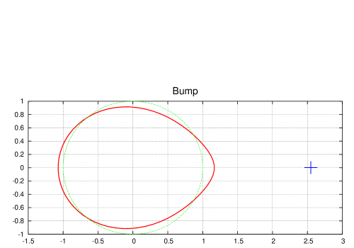
Figure 1: Curve (4.35), perturbed from initial unit circle (thin dotted line, in green, where available) by the flux, marked by (blue) cross on the right of the curve.

The computation of $t_{k}$, corresponding to this curve is done in appendix B. One sees that indeed $t_{k}=\frac{q}{k\zeta^{k}}$, where position of the flux $\zeta$ and its strength $q$ are given in terms of $a$ and $A$ by

$$\zeta=\frac{1}{\bar{a}}+\frac{A}{a(1-|a|^{2})},\quad q=\frac{{\bar{A}}}{{\bar{a}}^{2}}-\frac{|A|^{2}}{(1-|a|^{2})^{2}}$$ (4.36)

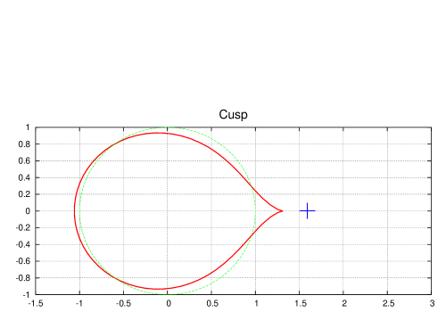
Figure 2: As flux (blue cross) moves closer to the curve (as compared to the figure 1) curve develops a cusp (corresponding to $z^{\prime}(w)=0$ in eq. (4.35)).

One may easily see that for $A=0$ curve (4.35) becomes a unit circle. The shape of the curve starts to change as one increases $a$ (keeping $A$ fixed for simplicity). It develops a bump in the direction of the flux (that is, the bump is centered along the ray, connecting origin with the position of the flux). It is shown on the figure 1. If we would move flux adiabatically around the curve, the bump would follow. This is the explicit realization of the equivalence between the (quasi)classical eigen-value (with position $\zeta$) and deformation of the Fermi-sea of the eigen-values [1, 2].

It is interesting to notice that the change of the shape of the curve depending on the trajectory of the classical eigen-value exhibits critical behavior. Namely, as one moves it closer and closer to the curve (i.e. decreases $\zeta$), bump not only grows but eventually becomes singular – the curve develops a cusp while the classical eigen-value is still the finite distance away from it (see figure 2).

This means that quasi-classical approximation is not applicable anymore. In this critical region quasi-classical approximation (dispersionless limit) is not valid anymore, and sub-leading effects become important. At this point the system changes drastically. The easiest way to see it, is to continue to move flux closer to the droplet. Then the curve would self-intersect, developing essentially the region with negative area (see figure 3).

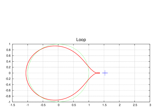
Figure 3: If one continues movement of the flux (blue cross) toward the curve (compared to fig. 1, and fig. 2, which are all done at the same scale) the curve self-intersects. Probably this should be considered as a creation of small separate droplet, but this is impossible to see in the quasi-classical approximation we are using in this paper.

Of course, it is not obvious that one can believe the classical analysis in the self-intersecting region. These features can also be seen analytically from eq. (4.35) and we refer the reader to the appendix B.

4.6 Shape of the non-compact Fermi sea in the presence of classical eigen-value

Similar to the previous section phenomena take place in the non-compact case. Indeed, the shape of Fermi sea is described by

$$x_{+}x_{-}=\mu+x_{+}S_{+}(x_{+})=\mu+\sum_{k=1}^{\infty}kt_{k}x_{+}^{k}+{\cal O}(\frac{1}{x_{+}})$$ (4.37)

Choosing as in the compact case $t_{k}$’s to be of the form $\frac{q}{k\zeta^{k}_{+}}$ we come to the situation similar to (4.32):

$$x_{+}x_{-}=\mu+\frac{qx_{+}}{x_{+}-\zeta_{+}}+{\cal O}(\frac{1}{x_{+}})$$ (4.38)

and similar representation for the $x_{-}$ representation with (in general different) coordinate of the flux $\zeta_{-}$. As in section 4.5, we can use a trick to find a form of the Fermi surface without finding explicitly $v_{\pm k}$. Namely, we find a parameterization $x_{+}(\omega)$, $x_{-}(\omega)$ which would satisfy eqs. (4.37)–(4.38) identically. In non-compact case it was used in [15]. There it was possible to find an ansatz for $x_{\pm}(\omega)$ because there was only finite number of $t_{\pm k}$. In the present case the number of $t_{k}$’s is infinite, but their particular form makes the procedure to be possible again.

We take the ansatz to be of the form:

$$x_{+}(\omega)=\omega-\frac{B\omega}{\omega+a_{+}};\quad x_{-}(\omega)=\frac{1}{\omega}-\frac{B}{1+a_{-}\omega}$$ (4.39)

where both $B$ and $a_{\pm}$ are positive and $0\leq\omega<\infty$. Substituting (4.39) into the eq. (4.37) one gets:

$$\zeta_{+}=-\frac{1}{a_{-}}-\frac{B}{1-a_{-}a_{+}};\quad\mu-\frac{q}{\zeta_{+}}=1-\frac{B}{a_{+}}$$ (4.40)

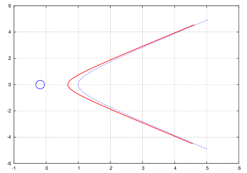
Figure 4: Deformation of the (non-compact) Fermi sea in the presence of the classical eigen-value. Circle (on the left) marks the position of the classical eigen-value. The deformed sea is the solid line. Hyperbola, to which it tends at infinities, is thin dotted (blue) line.

There is a particular difference between this case and the compact case of the previous section 4.5. For example, in non-compact case the whole Fermi sea was changing with introduction of the flux (see fig. 1). In this case, however, only the area close to the flux gets deformed (see fig. 4), while asymptotically ansatz (4.39) still gives

$$x_{+}x_{-}=\mu^{\prime}$$ (4.41)

– equation of unperturbed hyperbola.

Another difference with the compact case is the appearance of the cusp in case of only $t_{\pm 1}$ being non-zero [15]. In the compact case introduction of $t_{1},\bar{t}_{1}\neq 0$ would correspond to the shifted circle with no critical behavior possible.

Appearance of the cusp is a very intriguing phenomenon and its interpretation in the context of [1, 2] needs further clarification.

5 Discussion

In this section we briefly repeat the main results of this paper and discuss its open questions and relation to other works.

It has already been known for some time (c.f. e.g. [8]) that there is an intrinsic relation between $c=1$ MQM and normal matrix model (the latter describing, in view of [16], (integer) Quantum Hall system). However, precise relation between these two systems was not well understood. On the other hand, although known since early 90s, the fact that $1+1$ dimensional $c=1$ string theory is described by $0+1$ dimensional $c=1$ matrix quantum mechanics has not received a fully satisfactory explanation. From yet another point of view, current works on conjecture of [1] (see e.g. [11, 2] and many other recent references) were based on the widely accepted fact of duality between MQM and Liouville description of $c=1$ string theory [31].

This work adds new ingredients to all of these issues. First, it shows that results of [5, 8] can be better understood if one thinks about MQM as of analytic continuation of two-dimensional problem of the electron in the magnetic field. The one-dimensional problem of electrons in inverted harmonic potential appears from it as restriction to the “lowest Landau level”, as discussed in details in section 3.1. Analytically continued problem is two-dimensional as well, but lives in $1+1$ dimensions, rather than in $2+0$ as the magnetic system on the lowest Landau level does. This construction allows to give microscopic interpretation of the result of [8], where analytic continuation from normal matrix model to MQM was obtained on the level of partition functions. In [5] the wave-functions of fermions in non-trivial background, the shape of the Fermi-sea, and most of the results were obtained through orthogonalization procedure rather than via solution of an explicit Schroedinger equation. From the point of view of two-dimensional ($1+1$-dimensional) electrons in the magnetic (correspondingly, electric) field it corresponds to a choice of orthogonal basis on the “lowest Landau level” defined by equation ${\hat{H}}\Psi=0$. This is in turn equivalent to imposing an additional condition on the states on the lowest Landau level, namely the condition for them to be the eigen-states of some operator $L$ commuting with 2d Hamiltonian $\hat{H}$. That provides $1+1$-dimensional (rather than $0+1$ dimensional) interpretation of the fermionic system. The operator $L$ serves as $0+1$ dimensional Hamiltonian. Notice, that different choice of operator $L$ (i.e. different ordering on the space of solutions) would gives us different $0+1$ problem. This resembles a lot the problem of choice of time in general relativity or any generally covariant theory. This makes the problem of string theoretic interpretation of $1+1$ dimensional rather than MQM system very intriguing. Recall, that $1+1$-dimensional system of section 3.1 has known interpretation as strings in electric field (see e.g. [9]). We discussed it shortly in the section 3.1 and plan to return to this interpretation elsewhere. This direct string theoretic interpretation of MQM is in line with recent interpretation of MQM as of world-volume theory of tachyonic field of D-branes in c=1 string theory [1].

Next, we showed that CFT mechanism, developed recently for the Quantum Hall systems (as described in [29] and in sections 4.2–4.3) can be applied (in view of the aforementioned analytic continuation) to the $c=1$ MQM (or its two-dimensional equivalent) to reproduce all the ingredients of the conjecture [1]. In our formalism we are able to identify “classical” D-branes with the insertion of the “classical” flux and quantum D-brane with the action of operator $e^{\phi(\zeta)}$, such that $\psi(\zeta)=\langle e^{\phi(\zeta)}\rangle$. This shows, that, indeed, D-brane (described by fermion $\psi(\zeta)$) can be thought of as a soliton of MQM, built from various closed string excitations – pulses on the surface of Fermi-sea, whose creation/annihilation is described by the modes of the operator of the scalar field $\phi(\zeta)$. On the other hand, classical D-brane (flux, inserted in the position $\zeta(t)$) can be “dissolved” into the closed string background. We consider also explicit example of such “correspondence” between classical D-brane and closed string background and showed that one can expect critical phenomena there as well as processes of “creation” of D-branes.

The question of classical eigen-value needs some further investigation. We have mostly discussed the interpretation of classical eigen-value in case of compact droplet. The interpretation in non-compact case may be different, due to the fact, that we are only interested in deformations of vicinity of Fermi-surface. Nevertheless, classical eigen-value is described as small compact droplet also in this case and results of section 4.3 are also applicable. Thus we suggest that the classical D-brane in the non-compact case is a small compact droplet, placed outside the Fermi-sea and moving along the classical trajectory (For similar picture see e.g. [30]).

We should stress once again, that this is done in the way absolutely different from the usual approach of comparing results of computations in MQM with those of Liouville boundary CFT. It may well be that what is described here is a new, dual description of Liouville CFT (much simpler in some sense). We leave this investigation for the future.

It is also interesting to note that the description of D-branes, suggested in this paper is of more general nature. Indeed, recently the paper [34] has appeared, which suggests very similar realization of classical and quantum D-branes in the context of topological B-model (where $c=1$ string theory appears as a particular case).

Appendix A Schwarz function and harmonic moments of analytic curves

In this appendix we summarize briefly the results about the description of curves in terms of harmonic moments. The results can be found in [18, 20, 21] and in book [26].

Let ${\cal C}$ be an analytic curve in the plane, without self-intersections (for simplicity), and for simplicity “sufficiently close to circle” (see details in book [26]). Let denote by $D_{+}$ interior of curve and by $D_{-}$ - its exterior. For simplicity we assume that $z=0\in D_{+}$ and $z=\infty\in D_{-}$. Then one can define a set of harmonic moments of this curve, They are

– area

$$t_{0}=\frac{1}{\pi}\int_{D_{+}}d^{2}z=\frac{1}{2\pi i}\oint_{\cal C}dz{\bar{z}}$$ (A.1)

– moments of exterior

$$t_{k}=\frac{1}{2\pi ik}\oint_{\cal C}z^{-k}{\bar{z}}dz$$ (A.2)

– moments of interior

$$v_{k}=\frac{1}{2\pi i}\oint_{\cal C}z^{k}{\bar{z}}dz$$ (A.3)

and also logarithmic moment

$$v_{0}=\frac{1}{\pi}\int_{D_{+}}\log|z|^{2}d^{2}z$$ (A.4)

Then, one can construct the formal Laurent series, called the Schwarz function

$$S(z)=\sum\limits_{k=1}^{\infty}kt_{k}z^{k-1}+\frac{t_{0}}{z}+\sum\limits_{k=1}^{\infty}\frac{v_{k}}{z^{k+1}}$$ (A.5)

which defines the curve ${\cal C}$ via relation

$${\bar{z}}=S(z)$$ (A.6)

One can show, that eq. (A.5) has non-zero region of convergence in strip-like domain around the curve ${\cal C}$.

This statement can be reversed. Namely, if one has the function $S(z)$, formally defined via eq. (A.5) and if this function obeys so called unitarity condition in some region

$$\bar{S}(S(z))=z$$ (A.7)

for all $z$ in the domain of definition, then eq. (A.6) defines some curve. Without the condition (A.7) eq. (A.6) would define only a discrete set of points in the complex plane.

It should be noted, that set $t_{k}$, $v_{k}$ is over-determined. One can show that independent set of variable is all $t_{k}$ (all $v_{k}$’s are good set as well) and that

$$v_{k}=\displaystyle\frac{\partial F(t_{0},t_{k},\bar{t}_{k})}{\partial t_{k}},\quad k=0,1,\dots$$ (A.8)

where $F(t)$ is the logarithm of dispersionless tau-function of 2D Toda Lattice hierarchy. It is the same tau-function, which appears in the large $N$ limit of normal matrix model.

Appendix B Construction of the curve with one flux

We need a Schwarz function, which has one pole in the position $\zeta$ outside the contour. We are going to show that one can describe corresponding to such Schwarz function curve by the following conformal map:

$$z(w)=w+\frac{A}{a}+\frac{A}{w-a}=w+\frac{A}{a(1-\frac{a}{w})}$$ (B.1)

One should remember, that this is a map of exterior of the unit circle to the exterior of the curve and that it does not map interior of the circle into anything in the conformal way. To be the conformal map of exterior of the unit circle, one requires $|z^{\prime}(w)|\neq 0,\infty$, for $|w|\geq 1$. This leads to the following restrictions on parameters:

$$|a|<1,\quad|a\pm\sqrt{A}|<1$$ (B.2)

Indeed, according to the discussion above (see (4.34)), the Schwarz function, defined by

$$S(z(w))=\frac{1}{w}+\frac{\bar{A}}{\bar{a}({1}-\bar{a}w)}$$ (B.3)

has a single pole at the point $w_{f}=\frac{1}{\bar{a}}$, which means that position of the flux in the $z$-plane is given by

$$\zeta\equiv z(w_{f})=\frac{1}{\bar{a}}+\frac{A}{a(1-|a|^{2})}$$ (B.4)

Let us compute $t_{k}$ for the curve given by conformal map (B.1). According to definition (A.2)

$$t_{k}=\frac{1}{2\pi ik}\oint_{\cal C}z^{-k}{\bar{z}}dz$$ (B.5)

We assume that $\oint_{\cal C}\frac{dz}{z}=-2\pi i$.

$$t_{k} = \frac{1}{2\pi ik}\oint\limits_{|w|=1}z^{-k}(w){\bar{z}}(1/w)dz(w)$$

$$= \frac{1}{2\pi ik}\oint\limits_{|w|=1}\left(w+\frac{A}{a(w-a)}\right)^{-k}\left(\frac{1}{w}+\frac{\bar{A}}{\bar{a}(1-\bar{a}w)}\right)\left(1-\frac{A}{(w-a)^{2}}\right)dw$$

$$= \frac{1}{2\pi ik}\oint\limits_{|w|=1}\frac{(w-a)^{k}}{(w(w-a)+\frac{A}{a})^{k}}\left(\frac{1}{w}+\frac{\bar{A}}{\bar{a}^{2}}\frac{w}{\frac{1}{\bar{a}}-w}\right)\left(1-\frac{A}{(w-a)^{2}}\right)dw$$

We choose to pick up the poles outside the circle. There are two poles: at $w=1/\bar{a}$ (since $|a|^{2}<1$) and at $w=\infty$. We believe, that because of condition (B.2) poles of quadratic polynomial $w(w-a)+\frac{A}{a}$ are inside the unit circle and thus do not contribute. Also, one can see that in the case (B.1) residue at $w=\infty$ is equal to zero. Thus we have

$$t_{k}=\frac{1}{k}\left(\frac{1}{\bar{a}}+\frac{A}{\frac{1}{\bar{a}}-a}+\frac{A}{a}\right)^{-k}\frac{{\bar{A}}}{{\bar{a}}^{2}}\left(1-\frac{A}{(\frac{1}{\bar{a}}-a)^{2}}\right)=\frac{1}{k}\frac{q}{\zeta^{k}}$$ (B.7)

where $\zeta$ is given by eq. (B.4) and flux strength $q$ is defined as

$$q=z^{\prime}({\bar{a}}^{-1})\mathop{\mathrm{res}}_{w={\bar{a}}^{-1}}{\bar{z}}(w)=\frac{{\bar{A}}}{{\bar{a}}^{2}}\left(1-\frac{A\bar{a}^{2}}{(1-|a|^{2})^{2}}\right)=\frac{{\bar{A}}}{{\bar{a}}^{2}}-\frac{|A|^{2}}{(1-|a|^{2})^{2}}$$ (B.8)

The pole of $S(z)$ and its residue are position and the value of a flux. If we want flux to be real, this means that $\bar{A}/\bar{a}^{2}$ should be real as well.

The area of the droplet can be computed from (B.1), (B.3) as $t_{0}=\frac{1}{2\pi i}\oint\bar{z}(w^{-1})dz(w)$ i.e.

$$t_{0}=1-\frac{|A|^{2}}{(1-|a|^{2})^{2}}$$ (B.9)

We see, that $t_{0}$ is always real, regardless the values of parameters $a,A$, provided that conditions (B.2) are satisfied.

Now, let us look in more details at the situation when the cusp develops This corresponds to the critical point of the map: $z^{\prime}(w)=0$. Then $w=a\pm\sqrt{A}$ and $|w|=1$. Thus one can use eq. (B.1) to compute $z$ position of the cusp. It is given by

$$z_{cr}=z(a\pm\sqrt{A})=a\left(1+\frac{A}{a^{2}}\right)$$ (B.10)

On the other hand we can rewrite position of the flux $\zeta$ as

$$\zeta=a\left(\frac{1}{|a|^{2}}+\frac{A}{a^{2}(1-|a|^{2})}\right)$$ (B.11)

Due to comment after equation (B.8) we see that equation in parenthesis in both eqs. (B.10) and (B.11) are real. And thus, position of the flux and cusp lie on the same ray, coming from origin.

The distance between the critical point and the position of the flux is always positive.

References

- [1] J. McGreevy and H. Verlinde, “Strings from tachyons: The c = 1 matrix reloaded,” arXiv:hep-th/0304224;
- [2] J. McGreevy, J. Teschner and H. Verlinde, “Classical and quantum D-branes in 2D string theory,” arXiv:hep-th/0305194;
- [3] I. R. Klebanov, “String theory in two-dimensions,” arXiv:hep-th/9108019.
- [4] J. Polchinski, “Classical Limit Of (1+1)-Dimensional String Theory,” Nucl. Phys. B 362, 125 (1991);
- [5] S. Y. Alexandrov, V. A. Kazakov and I. K. Kostov, “Time-dependent backgrounds of 2D string theory,” Nucl. Phys. B 640 (2002) 119 [arXiv:hep-th/0205079] ;
- [6] D. J. Gross and I. R. Klebanov, “Vortices And The Nonsinglet Sector Of The C=1 Matrix Model,” Nucl. Phys. B 354 (1991) 459 ;
- [7] C. Itzykson and J. B. Zuber, “The Planar Approximation. 2,” J. Math. Phys. 21 (1980) 411 ;
- [8] S. Y. Alexandrov, V. A. Kazakov and I. K. Kostov, “2D string theory as normal matrix model,” Nucl. Phys. B 667 (2003) 90 [arXiv:hep-th/0302106];
- [9] B. Pioline and M. Berkooz, “Strings in an electric field, and the Milne universe,” JCAP 0311 (2003) 007 [arXiv:hep-th/0307280].
- [10] N. A. Nekrasov, “Milne universe, tachyons, and quantum group,” Surveys High Energ. Phys. 17 (2002) 115 [arXiv:hep-th/0203112].
- [11] I. R. Klebanov, J. Maldacena and N. Seiberg, “D-brane decay in two-dimensional string theory,” JHEP 0307 (2003) 045 [arXiv:hep-th/0305159];
- [12] S. Iso, D. Karabali and B. Sakita, “One-dimensional fermions as two-dimensional droplets via Chern-Simons theory,” Nucl. Phys. B 388 (1992) 700 [arXiv:hep-th/9202012];
- [13] A. Cappelli, C. A. Trugenberger and G. R. Zemba, “Infinite symmetry in the quantum Hall effect,” Nucl. Phys. B 396, 465 (1993) [arXiv:hep-th/9206027].
- [14] V. A. Kazakov and I. K. Kostov, “Loop gas model for open strings,” Nucl. Phys. B 386 (1992) 520 [arXiv:hep-th/9205059];
- [15] I. K. Kostov, “Integrable flows in c = 1 string theory,” J. Phys. A 36 (2003) 3153 [arXiv:hep-th/0208034];
- [16] O. Agam, E. Bettelheim, P. Wiegmann and A. Zabrodin, “Viscous fingering and a shape of an electronic droplet in the Quantum Hall regime”, arXiv:cond-mat/0111333;
- [17] A. Strominger, “A Matrix Model for AdS2,” arXiv:hep-th/0312194.
- [18] M. Mineev-Weinstein, P. B. Wiegmann and A. Zabrodin, “Integrable structure of interface dynamics,” Phys. Rev. Lett. 84, 5106 (2000) [arXiv:nlin.si/0001007].
- [19] A. Cappelli, G. V. Dunne, C. A. Trugenberger and G. R. Zemba, “Conformal symmetry and universal properties of quantum Hall states,” Nucl. Phys. B 398, 531 (1993) [arXiv:hep-th/9211071].
- [20] P. B. Wiegmann and A. Zabrodin, “Conformal maps and dispersionless integrable hierarchies,” Commun. Math. Phys. 213, 523 (2000) [arXiv:hep-th/9909147];
- [21] I. K. Kostov, I. Krichever, M. Mineev-Weinstein, P. B. Wiegmann and A. Zabrodin, “-function for analytic curves,” arXiv:hep-th/0005259;
- [22] M. Jimbo and T. Miwa, “Solitons And Infinite Dimensional Lie Algebras,” Publ. Res. Inst. Math. Sci. Kyoto 19, 943 (1983);
- [23] K. Takasaki and T. Takebe, “Integrable Hierarchies And Dispersionless Limit,” Rev. Math. Phys. 7, 743 (1995) [arXiv:hep-th/9405096];
- [24] M. Adler and P. van Moerbeke, “The spectrum of coupled random matrices,” Annals Math. 149, 921 (1999) [arXiv:hep-th/9907213].
- [25] L. L. Chau and O. Zaboronsky, “On the structure of correlation functions in the normal matrix model,” Commun. Math. Phys. 196, 203 (1998) [arXiv:hep-th/9711091];
- [26] P. J. Davis, The Schwarz function and its applications, The Carus Mathematical Monographs, No. 17, The Math. Assotiation of America, Bu alo, N.Y., 1974;
- [27] A. Boyarsky and O. Ruchayskiy, “Integrability in SFT and new representation of KP tau-function,” JHEP 0303, 027 (2003) [arXiv:hep-th/0211010];
- [28] P. Wiegmann, unpublished, 2002.
- [29] A. Boyarsky, V. Cheianov, and O. Ruchayskiy, “Microscopic derivation of the conformal field theory of excitation of Quantum Hall effect.”, to appear
- [30] A. Sen, “Open-closed duality: Lessons from matrix model,” arXiv:hep-th/0308068.
- [31] J. Polchinski, “What is string theory?,” arXiv:hep-th/9411028.
- [32] D. Gaiotto and L. Rastelli, “A paradigm of open/closed duality: Liouville D-branes and the Kontsevich model,” arXiv:hep-th/0312196
- [33] A. Boyarsky, B. Kulik and O. Ruchayskiy, “String field theory vertices, integrability and boundary states,” JHEP 0311, 045 (2003) [arXiv:hep-th/0307057].
- [34] M. Aganagic, R. Dijkgraaf, A. Klemm, M. Marino and C. Vafa, “Topological strings and integrable hierarchies,” arXiv:hep-th/0312085.