WIS/35/03-DEC-DPP
hep-th/0312209
December 2003

Abstract

We study the structure of closed timelike curves (CTCs) for the near horizon limit of the five dimensional BMPV black hole, in its overrotating regime. We argue that Bousso’s holographic screens are inside the chronologically safe region, extending a similar observation of Boyda et al. [1] for Gödel type solutions. We then extend this result to quite generic axisymmetric spacetimes with CTCs, showing that causal geodesics can’t escape the chronologically safe region. As a spin-off of our results, we fill a gap in the identification of all maximally supersymmetric solutions of minimal five dimensional supergravity, bringing this problem to a full conclusion.

1 Introduction

Much of the study of string theory solutions has been devoted to static backgrounds, and many static compactifications preserving at least a fraction of supersymmetry are relatively well understood. On the other hand, the status of time dependent solutions in string theory is much less satisfactory. Recently this situation has started to change, with increasingly more attention being paid to time-dependent backgrounds. Some of the approaches explored are time-dependent orbifolds of Minkowski space [2, 3, 4, 5], WZW models [6, 7], double analytical continuations of solutions [8] and others [9]. Together with the promise of bringing string theory one step closer to the observed world (after all, the Universe si muove), time dependent backgrounds can present new seemingly pathological features, absent from static compactifications. For instance, in time-dependent orbifolds, new kinds of singularities appear, and both time-dependent orbifolds of Minkowski space and WZW models can have closed null curves [2, 3] or closed timelike curves (CTCs) [10, 6, 4].

At this stage, the rules to deal with these pathologies are not clear, but one might hope that by learning how string theory copes with them, we can gain a better understanding of the theory, beyond the realm of static solutions. In particular, the possible existence of closed timelike curves in string theory raises many interesting conceptual issues: does string theory actually allow solutions with closed timelike curves, or do they have to be discarded? Is the chronology protection conjecture [11] realized in string theory? If so, what is the mechanism behind it? Typically, for time-dependent backgrounds we currently lack the tools to address these questions.

A possible route to make progress is to consider stationary non-static solutions in supergravity theories, which occupy an intermediate position between static and time-dependent backgrounds. There are plenty such solutions that are supersymmetric and everywhere regular, and yet present CTCs. Among those, the solutions of five dimensional supergravity (and their uplifts to ten dimensions), have received special attention. This is in part due to the characterization of all supersymmetric solutions of minimal five dimensional supergravity [13]. Among the maximally supersymmetric solutions, one finds a 5d generalization of the Gödel solution and the near horizon limit of the rotating BMPV [14] black hole (NH-BMPV). Both of those solutions present closed timelike curves, at least in a range of parameters.

The Gödel type solution and its ten dimensional cousins have been studied in considerable detail [1, 15, 16, 17, 18, 19, 20, 21, 22, 23, 24]. Of particular relevance for the present work, is the observation [1] that for Gödel type solutions, although there are closed timelike curves passing through every point in spacetime, if we apply Bousso’s prescription for holographic screens [25] to these backgrounds, the induced metric on the resulting screen is free of closed timelike curves. This gives place to the speculation that there might be a holographic description despite the presence of closed timelike curves on the classical background.

In this work, we consider the other maximally supersymmetric solution of $d=5$ minimal sugra with CTCs, the near horizon limit of the overrotating BMPV black hole. The CTCs of the full overrotating BMPV solution were studied in [26]. We show that the pattern of CTCs is very similar to that of the Gödel solution, and again Bousso’s holographic screen is inside the chronologically safe region. As a welcome bonus from our study, we bring to a full conclusion the identification of all maximally supersymmetric solutions of 5d minimal supergravity, filling a gap in the discussion of [13] (see also [27]). Namely, we explicitly show that the three solutions that were left unidentified in [13] correspond to the near horizon limit of the BMPV solutions, in the underrotating, critical and overrotating cases, respectively.

After studying this five dimensional example in quite some detail, we further consider more general metrics in arbitrary dimensions, where closed timelike curves appear because of overrotation in different planes, and show quite generally that causal (timelike or null) geodesics cannot escape the chronologically safe region surrounding a given observer. As a corollary, the corresponding holographic screens are inside the chronologically safe regions, and the induced metrics have no CTCs.

In this work we are concerned mostly with properties of classical metrics with CTCs. It is worth noting that for some of the ten dimensional sugra solutions, there are probe computations [28, 29, 16] suggesting that these backgrounds actually can’t be built in string theory.

The structure of the paper is as follows. In Section 2 we review the status of vacua of five dimensional supergravity. In Section 3 we study in detail the NH-BMPV solution. After defining the notions we are going to use, like optical horizon or chronologically safe region, we describe in detail the structure of closed timelike curves in the NH-BMPV background, and show that the optical horizon coincides with the boundary of the chronologically safe region. In Section 4 we extend the study of optical horizons and chronologically safe regions to quite generic static and axisymmetric spacetimes, and we find that the optical horizon never extends beyond the chronologically safe region; furthermore, it generically coincides with the boundary of said region, although we show examples where this is not the case. As a corollary, Bousso’s holographic screen for all these spacetimes is inside the chronologicallty safe region, and the induced metric on this screen has no CTCs. Finally, we state our conclusions in Section 5.

2 NH-BMPV and the Complete identification of $d=5$ Vacua

One of the main purposes of this paper is the investigation of CTCs in the background of the near horizon limit of the five dimensional extreme rotating black hole (for short, we will henceforth use the acronyms “BMPV black hole” for this black hole spacetime [14] and “NH-BMPV” for its near-horizon limit). This near horizon spacetime is homogeneous [35] and maximally supersymmetric and, when the “rotational” parameter $j$ (to be defined below) exceeds a certain critical value, it develops naked CTCs. We will start with a detailed study of this spacetime itself. This, in turn, will provide us with the answer to the problem of the identification of all maximally supersymmetric solutions of minimal five dimensional supergravity, an issue on which we now elaborate.

All bosonic solutions of pure $\mathcal{N}=2$ (eight supercharges) five dimensional supergravity preserving some fraction of supersymmetry were characterized in [13]. In particular, all maximally supersymmetric solutions (which henceforth we will call “vacua”) were obtained, and it was found that these include the following spacetimes:

• $AdS_{2}\times S^{3}$, which also arises as the near horizon limit of the non-rotating five dimensional extreme black hole [32].

• $AdS_{3}\times S^{2}$, which is the near horizon limit of the extreme string solution [36].

• The spacetime arising as the near horizon limit of the rotating BMPV black hole.

• The homogeneous plane wave found in [37].

• A five dimensional analogue of the Gödel universe.

In addition to those, three more solutions satisfying the necessary conditions for maximal supersymmetry were also found in [13], but they were not identified neither explicitly shown to be maximally supersymmetric (see Sections 5.3 and 5.4 of [13]). Subsequently, those unidentified solutions where retrieved and shown to be indeed maximally supersymmetric in [27], where a complete classification of all five dimensional vacua was obtained by dimensional reduction from six dimensions, but, again, no explicit identification of them was provided. In [13] and [27] the possibility that they might belong to the NH-BMPV family was already anticipated, and below we are going to show that this is indeed the case. In fact, we shall see that these solutions correspond to the NH-BMPV spacetime in the “underrotating”, “critical” (having closed lightlike curves) and “overrotating” (having CTCs) cases, resepctively.

Among the five dimensional spacetimes in the list above, two of them exhibit CTCs. These are the Gödel universe and, generically, the NH-BMPV spacetime. It was shown in [39] that most maximally supersymmetric vacua of supergravity theories in dimensions $d=4,5$ and 6 with eight supercharges can be related by uplift and dimensional reduction. The fact that this has to be so for the $d=5\leftrightarrow d=6$ vacua was explained in [27]. What we are going to see below is that the emergence of CTCs in five dimensions can be understood from the identifications one makes in the six dimensional vacua [27, 40]. This approach is what, following [27], will in the end provide us with an answer to the question about the complete identification of maximally supersymmetric solutions in five dimensions. In particular, we will focus on the near horizon BMPV family. CTCs in the Gödel case have already been studied in the literature from several perspectives [41, 15, 16, 17, 18, 19, 20, 21, 23] and, concerning its lift to six dimensions, it was already pointed out in [27] that it yields the maximally supersymmetric six dimensional homogeneous wave of [37]. As we will see below, the 6-dimensional lifts of the whole near horizon BMPV family yield $AdS_{3}\times S^{3}$, but with different global identifications dictated by the causal structure of the five dimensional cases.

Next we describe the NH-BMPV family and its lift to six dimensions. We will organize the possible cases according to the causal properties of the five dimensional solutions. From the six dimensional perspective they provide different Hopf fibrations of the $AdS_{3}$ factor, which we will call, respectively, “spacelike”, “timelike” and “lightlike”. We refer the interested reader to Appendix A for a more detailed discussion on those.

2.1 The Near Horizon BMPV Family

The near horizon BMPV black hole solution can be presented as:

$$\left\{\begin{array}[]{r@{\;}c@{\;}l}ds^{2}&=&\displaystyle{-\biggl{(}\frac{r}{R}\;dt-Rj(d\chi+\cos\theta\;d\varphi)\biggr{)}^{2}+\frac{R^{2}}{r^{2}}\;dr^{2}+4R^{2}d\Omega_{(3)}^{2}}\,,\\[10.76385pt] F&=&\displaystyle{-\frac{\sqrt{3}}{R}\;dt\wedge dr+\sqrt{3}Rj\sin\theta\;d\theta\wedge d\varphi}\,,\end{array}\right.$$ (2.1)

where

$$d\Omega_{(3)}^{2}=\frac{1}{4}\Bigl{(}d\Omega_{(2)}^{2}+(d\chi+\cos\theta\;d\varphi)^{2}\Bigr{)}=\frac{1}{4}\Bigl{(}d\theta^{2}+\sin^{2}\theta\;d\varphi^{2}+(d\chi+\cos\theta\;d\varphi)^{2}\Bigr{)}$$

gives the usual Hopf-fibered form of the unit $S^{3}$ (i.e., the angles $\theta$, $\varphi$ and $\chi$ take values in $[0,\pi]$, $[0,2\pi]$ and $[0,4\pi]$, respectively). This solution (up to a reparametrization $r\rightarrow r^{2}$ of the radial coordinate and with a different choice for the parameters) is the near horizon limit of the five dimensional supersymmetric extreme rotating black hole as given in [34]. The angular momentum of the black hole solution is set by the dimensionless parameter $j$. For $j>1$, (2.1) has closed timelike curves, while for $j=1$ there are closed lightlike curves. We will now look at the six dimensional lift of these solutions in the different ranges of $j$. For $j<1$ we will write $j=\sin\xi$, while for $j>1$ we will parametrize it as $j=\cosh\xi$.

2.2 Six Dimensional Lifts of NH-BMPV

Let us first record here the lifting rules to six dimensions. For a general five dimensional solution given by a line element $ds^{2}$ and two-form $F=dA$, the uplifting rules to the minimal six dimensional supergravity theory (whose bosonic field content is given by the six dimensional metric and an anti-self-dual three form $H=dB$) are given by [39]:

$$\left\{\begin{array}[]{r@{\;}c@{\;}l}ds_{(6)}^{2}&=&\displaystyle ds^{2}+\biggl{(}dw+\frac{1}{\sqrt{3}}A\biggr{)}^{2}\,,\\[8.61108pt] B_{\mu w}&=&\displaystyle\frac{1}{\sqrt{3}}A_{\mu}\,,\end{array}\right.$$ (2.2)

where $w$ is the “sixth coordinate”. The remaining components of the two-form potential can be calculated from the anti-self-duality constraint. All five and six dimensional solutions that we will describe have, respectively, nontrivial two- and three-form fields. We will omit from now on the expressions for the gauge fields, since our main interest concerns the causal structure and the global identifications of the spacetime metrics.

Six Dimensional Lift for $j<1$

We first look at the case $j<1$, which has no causal singularities. After writing $j=\sin\xi$ and performing the rescaling

$$t\rightarrow\cos\xi\;t$$ (2.3)

we can write the five dimensional metric as:

$$ds^{2}=-\frac{r^{2}}{R^{2}}\;dt^{2}+\frac{R^{2}}{r^{2}}\;dr^{2}+R^{2}d\Omega_{(2)}^{2}+R^{2}\cos^{2}\xi\biggl{(}d\chi+\cos\theta\;d\varphi+\tan\xi\frac{r}{R^{2}}\;dt\biggr{)}^{2}\,,$$ (2.4)

making clear that this spacetime is a $\mathop{\kern 0.0pt\mathrm{U}}\nolimits(1)$ fibration over $AdS_{2}\times S^{2}$. In fact, it was shown in [35] that the $j<1$ NH-BMPV spacetime is homogeneous and, locally,

$$\mbox{NH-BMPV}\simeq\frac{\mathop{\kern 0.0pt\mathrm{SO}}\nolimits(2,1)\times\mathop{\kern 0.0pt\mathrm{SO}}\nolimits(3)}{\mathop{\kern 0.0pt\mathrm{U}}\nolimits(1)_{\xi}}\,,$$

with $\xi$ determining the relative weight of the $\mathop{\kern 0.0pt\mathrm{U}}\nolimits(1)$ action on each factor. This already indicates that we are dealing with a quotient of $AdS_{3}\times S^{3}$ and explains why the $j<1$ subfamily admits a local metric which interpolates between those of $AdS_{2}\times S^{3}$ at $\xi=0$ and $AdS_{3}\times S^{2}$ at $\xi=\pi/2$ (this is not apparent in these coordinates, though — see the discussion in [39, 35]). This interpolation has also been pointed out in [13, 27]. One of the things that we will clarify later on is the fact that, although the $j=0$ case is indeed $AdS_{2}\times S^{3}$, the $j=1$ case is not $AdS_{3}\times S^{2}$. Only the $j\to 1$ limit of the $j<1$ subfamily admits a metric which is locally that of $AdS_{3}\times S^{3}$. In fact, we will show that the $AdS_{3}\times S^{2}$ vacuum is not smoothly connected to the NH-BMPV family. The fact that the $j=1$ limit of both the underrotating and overrotating NH-BMPV subfamilies (Eqns. (2.4) and (2.9)) is singular can be interpreted as an indication of the peculiar properties of the $j=1$ case.

After these considerations about this five dimensional spacetime, let us write its lift to six dimensions. Using the KK-rules (2.2) and further defining the rotated angles

$$\pmatrix{u\cr\psi}=\pmatrix{\sin\xi&\cos\xi\cr-\cos\xi&\sin\xi}\pmatrix{\cos\xi\;\chi\cr w/R}\,,$$ (2.5)

we get the six dimensional metric

$$ds_{(6)}^{2}=-\frac{r^{2}}{R^{2}}\;dt^{2}+\frac{R^{2}}{r^{2}}\;dr^{2}+R^{2}\biggl{(}du+\frac{r}{R^{2}}\;dt\biggr{)}^{2}+4R^{2}d\Omega_{(3)}^{2}\,,$$ (2.6)

where now $4d\Omega_{(3)}^{2}=d\Omega_{(2)}^{2}+(d\psi-\cos\theta\;d\varphi)^{2}$. We verify (see Appendix B) that this spacetime is locally $AdS_{3}\times S^{3}$, and that the metric in this form does no longer depend on the “rotational” parameter $j$, since its six dimensional meaning is the choice of the KK compactification direction. Using the coordinate transformation given by (B.3) we can write this metric in global coordinates and see that the $AdS_{3}$ factor precisely corresponds to the spacelike Hopf fibration of $AdS_{3}$ over $AdS_{2}$ (along the coordinate that we now call $\tilde{\psi}$) discussed in Appendix A:

$$ds_{(6)}^{2}=-R^{2}\cosh^{2}\frac{\rho}{R}\;d\tau^{2}+d\rho^{2}+R^{2}\biggl{(}d\tilde{\psi}+\sinh\frac{\rho}{R}\;d\tau\biggr{)}^{2}\,+4R^{2}d\Omega_{(3)}^{2}.$$ (2.7)

It is worth mentioning that, to make contact with five dimensions, we have to keep the “sixth coordinate” compact. When keeping $w$ compact, its periodicity has to be chosen so that the period of $\psi$ is $4\pi$ in order to have a regular space. This automatically sets the period of $\tilde{\psi}$ and ensures a regular space and a well-defined $\mathop{\kern 0.0pt\mathrm{U}}\nolimits(1)$ action along $\tilde{\psi}$ whenever $j<1$. Note that the Hopf direction $\tilde{\psi}$ is spacelike. It is crucial to take this point of view on the compactness of the six dimensional backgrounds in order to make contact with the analysis that we will perform in Section 2.3 and, of course, it also applies to the $j>1$ and $j=1$ cases.

Six Dimensional Lift for $j>1$

Next we look at the case $j>1$, which has CTCs. After setting $j=\cosh\xi$ and the rescaling

$$t\rightarrow\sinh\xi\;t\,,$$ (2.8)

one can write the metric as

$$ds^{2}=\frac{r^{2}}{R^{2}}\;dt^{2}+\frac{R^{2}}{r^{2}}\;dr^{2}+R^{2}d\Omega_{(2)}^{2}-R^{2}\sinh^{2}\xi\biggl{(}d\chi+\cos\theta d\varphi-\coth\xi\frac{r}{R^{2}}\;dt\biggr{)}^{2}\,.$$ (2.9)

We can see that this spacetime is a $\mathop{\kern 0.0pt\mathrm{U}}\nolimits(1)$ fibration over the hyperbolic plane $\mathbb{H}_{2}$ times the sphere $S^{2}$. The six dimensional lift now reads:

$$ds_{(6)}^{2}=\frac{r^{2}}{R^{2}}dt^{2}+\frac{R^{2}}{r^{2}}dr^{2}-R^{2}\biggl{(}du+\frac{r}{R^{2}}dt\biggr{)}^{2}+R^{2}d\Omega_{(3)}^{2}\,,$$ (2.10)

where $d\Omega_{(3)}^{2}$ is as in (2.6), but now with the “boosted” angles defined as:

$$\pmatrix{u\cr\psi}=\pmatrix{\cosh\xi&-\sinh\xi\cr-\sinh\xi&\cosh\xi}\pmatrix{\sinh\xi\;\chi\cr w/R}\,.$$ (2.11)

This spacetime is again $AdS_{3}\times S^{3}$ locally, but global identifications are now completely different. By using the coordinate transformation (B.5) we can write this in global coordinates and find it to coincide with the timelike Hopf fibration of the $AdS_{3}$ factor:

$$ds_{(6)}^{2}=R^{2}\cosh^{2}\frac{\rho}{R}\;d\tau^{2}+d\rho^{2}-R^{2}\biggl{(}d\tilde{\psi}+\sinh\frac{\rho}{R}\;d\tau\biggr{)}^{2}\,+4R^{2}d\Omega_{(3)}^{2}$$ (2.12)

(compare to (2.7)). The $\xi$-dependence also goes away in the six dimensional spacetime. Again, we can always choose the appropriate period for $w$ in order to have a smooth space with a well-defined $\mathop{\kern 0.0pt\mathrm{U}}\nolimits(1)$ action along the Hopf direction $\tilde{\psi}$, which now is timelike.

Six Dimensional Lift for $j=1$

Note that (2.4) and (2.9) are, in principle, not smoothly connected in parameter space, since the above rescalings of the time coordinate are not allowed when $j=1$ (and, in fact, both five dimensional metrics as written below are singular in that limit). The lift of (2.1) when $j=1$ gives the metric:

$$ds_{(6)}^{2}=2r(d\chi-d\psi)dt+\frac{R^{2}}{r^{2}}dr^{2}+R^{2}d\Omega_{(3)}^{2}\,,$$ (2.13)

where now $4d\Omega_{(3)}^{2}=d\Omega_{(2)}^{2}+(d\psi-\cos\theta d\varphi)^{2}$. To get this form we have just defined

$$w\rightarrow R\psi\,$$ (2.14)

after the uplift. Putting $\tilde{\psi}\equiv\chi-\psi$ we make contact with the $AdS_{3}$ metric (B.1) in the case $\alpha=0$. If we further define

$$\rho=R\;\log\frac{r}{R}\,,$$

we have the metric

$$ds_{(6)}^{2}=2e^{\rho/R}dtd\tilde{\psi}+d\rho^{2}+4R^{2}d\Omega_{(3)}^{2}\,,$$ (2.15)

which, from (A.15), we can again identify locally with $AdS_{3}\times S^{3}$, but now with the $AdS_{3}$ factor given by the lightlike Hopf fibration discussed in Appendix A. We see that, also in this case, we have a well-defined $\mathop{\kern 0.0pt\mathrm{U}}\nolimits(1)$ action along the null coordinate $\tilde{\psi}$ with period equal to $4\pi$.

2.3 Classification and Reduction from 6 Dimensions

We have seen that the near horizon limits of the five dimensional extreme rotating black hole can be related to reductions of $AdS_{3}\times S^{3}$ with various identifications, and so far we have related their explicit local metrics in five and six dimensions. However, the relevant piece of information in order to analyze both the classification of five dimensional vacua and their causal structure concerns global issues. We now elaborate on this, following almost in parallel the lines and notation established in [27].

We have shown in the preceding section that the $j<1$, $j>1$ and $j=1$ cases of the NH-BMPV family, when lifted to six dimensions, can be seen locally as quotients

$$\frac{AdS_{3}\times S^{3}}{\mathop{\kern 0.0pt\mathrm{U}}\nolimits(1)}\,,$$ (2.16)

but with different choices for the direction of the $\mathop{\kern 0.0pt\mathrm{U}}\nolimits(1)$. It turns out that this is really helpful in order to understand these five dimensional vacua, since all possible maximally supersymmetric solutions in $d=5$ were shown in [27] to be given by all possible “spacelike quotients” of all possible six dimensional vacua, such as $AdS_{3}\times S^{3}$. All six dimensional vacua are given by Lorentzian Lie groups [27], and by “spacelike quotients” we mean those which are in one-to-one correspondence with the different spacelike one-parameter subgroups of these six dimensional vacua. In order to see this, what we are going to do next is, in a sense, the opposite analysis of the one in the last Section. We are going to “dimensionally reduce” $AdS_{3}\times S^{3}$, investigating the properties of all possible spacelike quotients and paying special attention to global aspects. To do so, we will identify $AdS_{3}$ with the universal cover of $\mathop{\kern 0.0pt\mathrm{SL}}\nolimits(2)$, while $S^{3}$ will be seen as $\mathop{\kern 0.0pt\mathrm{SU}}\nolimits(2)$. From the point of view of $AdS_{3}$ — when seen (as usual) as its universal covering — all freely acting 1-parameter subgroups are noncompact. So, strictly speaking, we have to look at quotients of the kind:

$$\frac{\widetilde{\mathop{\kern 0.0pt\mathrm{SL}}\nolimits}(2)\times\mathop{\kern 0.0pt\mathrm{SU}}\nolimits(2)}{\mathbb{R}}\,.$$ (2.17)

We will take the convention that $\mathbb{R}$ always acts by a right action of $\widetilde{\mathop{\kern 0.0pt\mathrm{SL}}\nolimits}(2)\times\mathop{\kern 0.0pt\mathrm{SU}}\nolimits(2)$ on itself. The direction in the second factor can always be chosen to be proportional to a fixed Lie algebra generator ($\kappa$, say) of $\mathop{\kern 0.0pt\mathit{su}}\nolimits(2)$. However, in $\widetilde{\mathop{\kern 0.0pt\mathrm{SL}}\nolimits}(2)$ we can choose inequivalent generators. Let us denote, as in [27], by $\sigma$, $\nu$ and $\tau$ a spacelike, lightlike and timelike generator of $\mathop{\kern 0.0pt\mathit{sl}}\nolimits(2)$ respectively; e.g. given by $\sigma=\hat{\tau}^{1}$, $\tau=\hat{\tau}^{2}$, $\nu=\hat{\tau}^{1}+\hat{\tau}^{2}$ (see Appendix A for notation). Then the possible spacelike generators are of the form (1) $a\sigma+b\kappa$, (2) $\nu+\kappa$ or (3) $a\tau+b\kappa$, where $a$ and $b$ are arbitrary real weights, although one must realize that in the last case we need $b^{2}>a^{2}>0$ in order to have a spacelike subgroup. For the first case we will consider separately the cases ($1^{\prime}$) $\sigma$ and ($1^{\prime\prime}$) $\kappa$.

To see the $d=5$ solutions as genuine KK-reductions from $d=6$ we need to describe them not as a quotient by $\mathbb{R}$, but rather as a quotient by $\mathop{\kern 0.0pt\mathrm{U}}\nolimits(1)$. Note that, except for the case ($1^{\prime}$), the subgroup always acts on $S^{3}$. As this space is compact, there is a $\mathbb{Z}$ subgroup that acts trivially on this factor. Therefore this $\mathbb{Z}$ subgroup only acts non trivially on $AdS_{3}$ and we can divide it out separately. That is, we can write:

$$\frac{AdS_{3}\times S^{3}}{\mathbb{R}}=\biggl{(}\frac{AdS_{3}}{\mathbb{Z}}\times S^{3}\biggr{)}/\mathop{\kern 0.0pt\mathrm{U}}\nolimits(1)\,,$$ (2.18)

the $\mathop{\kern 0.0pt\mathrm{U}}\nolimits(1)$ here being the one acting along the “sixth coordinate” in the different lifts (2.7), (2.12) and (2.15), i.e. the $\mathop{\kern 0.0pt\mathrm{U}}\nolimits(1)$ in the local description provided by (2.16). The $\mathbb{Z}$ action is of course generated by the same Killing vector as $\mathbb{R}$, but with a period dictated by the one in $S^{3}$. For example, if $\kappa$ is normalized such that it has period $2\pi$ on $S^{3}$, we find that the period of $\mathbb{Z}$ on $AdS_{3}$ is $2\pi a/b$ in case (1), etc. In case ($1^{\prime}$) the Killing vector acts only on $AdS_{3}$, and therefore we could have chosen any $\mathbb{Z}$ subgroup to begin with. In the case ($1^{\prime\prime}$) we are forced from the start to have an action by $\mathop{\kern 0.0pt\mathrm{U}}\nolimits(1)$ instead of $\mathbb{R}$, as it acts only on the compact space $S^{3}$. The different possibilities and the relations to extremal black holes and $d=4$ Robinson-Bertotti (to be discussed below) are summarized in Table 1.

case	generator	$j$ range	NH of $d=5$ extremal BH	$d=4$ reduction to RB
(1)	$a\sigma+b\kappa$	$0<j<1$	physical rotating	dyonic $j=\sin\xi$
($1^{\prime}$)	$\sigma$	$j=0$	non-rotating ($AdS_{2}\times S^{3}$)	electric
($1^{\prime\prime}$)	$\kappa$		NH of black string ($AdS_{3}\times S^{2}$)	magnetic
(2)	$\nu+\kappa$	$j=1$	critical rotating
(3)	$a\tau+b\kappa$	$j>1$	overrotating

Table 1: The possible reductions of $AdS_{3}\times S^{3}$ and their relation to $d=5$ and $d=4$ maximally supersymmetric solutions.

The identification of these quotients with the supergravity solutions belonging to the NH-BMPV family follows from the spacelike, timelike or null properties of the identifications discussed here and those of the six dimensional lifts discussed in the previous section. The identification of case ($1^{\prime\prime}$) with $AdS_{3}\times S^{2}$ is obvious.

Let us now analyze how these different solutions are connected. We can continuously go from case (1) to case ($1^{\prime}$). Indeed, thought of as the action on a cylinder (the noncompact direction being that in $AdS_{3}$, the circle being in $S^{3}$, and the one-parameter subgroup being a line winding the cylinder), the only thing that happens when $j\to 0$ (or $b\to 0$) is that the action has a longer and longer period over the noncompact direction — the endpoint is a decompactification (which is very much like the limit of a circle to the real line). However, we can not continuously go from case (1) to case ($1^{\prime\prime}$), even though the Killing vector changes continuously. The reason is that the quotient group goes discontinuously from $\mathbb{R}$ to $\mathop{\kern 0.0pt\mathrm{U}}\nolimits(1)$. If we try to take the limit, the extra factor of $\mathbb{Z}$ acting on $AdS_{3}$ will reduce the circle (the one which should arise after the identification) to zero size, and make a degenerate limit. A similar reasoning holds for the relation to case (3), taking $a\to 0$: this is not a well defined limit and therefore ($1^{\prime\prime}$) is, again, not continuously connected to case (3).

When from e.g. case (1) we take $j\to 1$, what we should do is to zoom into the circle that is vanishing. The way to do this is as in Matrix theory, by applying a large boost, which becomes infinite in the $j=1$ limit. Then the zero-size circle is boosted to a finite size (but zero proper length) lightlike circle, and what we end up with is case (2). Therefore we find that case (2) is continuously connected to case (1) and, similarly, case (2) is also continuously connected to case (3). An indication of this fact is that (2.1) provides a single, never degenerate metric for the whole NH-BMPV family.

Summarizing, we find that all solutions live in the same family, except for case ($1^{\prime\prime}$). This is why, as already advanced, the $AdS_{3}\times S^{2}$ vacuum cannot be continuously connected to the NH-BMPV family. Note that this can be physically understood from the BPS configurations that give rise to these near horizon spacetimes: $AdS_{3}\times S^{2}$ is the only solution that is not the near-horizon limit of a BH, but rather of the black string.

Finally, let us mention that, from this six dimensional point of view, the emergence of closed lightlike curves and CTCs in cases (2) and (3) is clear: as discussed in [27] (see also [42] for similar reductions), this is due to the null and timelike character of the Killing vectors $\nu$ and $\tau$ generating the identifications. Even if the “sixth circle” is spacelike, it is enforcing identifications inside the lightcone in the dimensionally reduced space.

Relation to Four Dimensional Robinson-Bertotti Spacetimes

We have seen how the NH-BMPV family is related to $AdS_{3}\times S^{3}$ in six dimensions. In [39] it was shown that five dimensional vacua are also related to four dimensional ones since, in general, they can be dimensionally reduced to four dimensions without breaking any supersymmetry, hence giving rise to vacua of pure $\mathcal{N}=2$, $d=4$ supergravity theory. In particular, it was shown that the $j<1$ NH-BMPV family and the $AdS_{3}\times S^{2}$ vacuum, when reduced to $d=4$, both give rise to near horizon limits of Robinson-Bertotti spacetimes (which are the near horizon limit of the Reissner-Nordström black holes and whose metrics are those of $AdS_{2}\times S^{2}$). In $d=4$ we have a whole family of RB spacetimes due to four dimensional electric-magnetic duality. In this way, the $j=0$ case ($AdS_{2}\times S^{3}$) gives rise to the purely electric RB solution, while the $j<1$ BH-BMPV gives rise to a general dyonic RB spacetime (with ratio between electric and magnetic charges precisely determined by $j=\sin\xi$, where now $\xi$ exactly coincides with the angle parametrizing electric-magnetic duality “rotations” in four dimensions). On the other hand, the lift of the purely magnetic RB solution was shown in [39] to correspond to $AdS_{3}\times S^{2}$. These results are summarized in Table 1. It is instructive to take a closer look at this, since we have just shown that the five dimensional $AdS_{3}\times S^{2}$ vacuum is not continuously connected to the $j<1$ NH-BMPV family, while in four dimensions electric-magnetic duality of course interpolates smoothly between the purely electric and purely magnetic cases.

In four dimensions the situation is as follows. It is a well-known fact that electric-magnetic duality acts locally on the gauge invariant field strength, but in a highly nonlocal way on the gauge potential. Purely electric and purely magnetic RB spacetimes are smoothly connected when written in terms of the field strength. However, when written in terms of the gauge potential (or more conveniently the dual gauge potential $\tilde{A}_{(4)}$), the situation is more subtle.

When we approach the monopole configuration in the limit $j\to 1$, the gauge transformation for $\tilde{A}_{(4)}$ needed to remove the Dirac string singularity — which is a global issue — has to be periodically identified with a period which is vanishing in the limit. If one wishes to couple the four dimensional theory to magnetic charges, it is easily verified that what is happening is that the unit of magnetic charge diverges in the limit. Only in the purely magnetic case, when the dual potential $\tilde{A}_{(4)}$ is “purely electric”, everything is well defined.

From the five dimensional point of view we are forced to use $\tilde{A}_{(4)}$, as we can not write the five dimensional metric in terms of gauge invariant quantities. The metric in five dimensions is in fact given by

$$ds^{2}\sim ds_{(4)}^{2}+\left(dx^{5}+\tilde{A}_{(4)}\right)^{2}\,,$$

and hence we see that the periodicity of the gauge field in four dimensions corresponds to the periodicity of the fifth coordinate $x^{5}$.

Explicit Identification of Five Dimensional Solutions

The considerations above show that all possible reductions of the 6-dimensional $AdS_{3}\times S^{3}$ vacuum are in the NH-BMPV family. Since all possible inequivalent reductions of the other nontrivial 6-dimensional vacuum (namely, the homogeneous plane wave of [37]) give the maximally supersymmetric 5-dimensional plane wave or the Gödel universe [27], we conclude that the different NH-BMPV cases complete all possible five dimensional vacua. We have thus identified them. However, for the sake of completeness, let us explicitly show that the different cases of NH-BMPV can be related to the three unidentified solutions of [13]. For convenience, we now set to unit the scale parameter $R$.

$\bullet$ $j<1$:

Starting from the solution (2.4) for $j<1$ and using essentially the coordinate transformation (B.3), followed by $R=\sinh\rho$, we find the solution (5.118) of [13],

$$ds^{2}=-(R^{2}+1){dt^{\prime}}^{2}+\frac{dR^{2}}{R^{2}+1}+\cos^{2}\xi(d\psi+\tan\xi\;Rdt^{\prime}+\cos\theta\;d\phi)^{2}+d\theta^{2}+\sin^{2}\theta\;d\phi^{2}\,.$$ (2.19)

$\bullet$ $j>1$:

Starting from the solution (2.9) for $j>1$ and using the coordinate transformation (B.9), followed by $R=\cosh\rho$, we find the solution (5.113) of [13],

$$ds^{2}=\frac{dR^{2}}{R^{2}-1}+(R^{2}-1){d\chi}^{2}-\sinh^{2}\xi(d\psi-\coth\xi\;Rd\chi+\cos\theta\;d\phi)^{2}+d\theta^{2}+\sin^{2}\theta\;d\phi^{2}\,.$$ (2.20)

$\bullet$ $j=1$:

Finally, starting from the $j=1$ solution as given by (2.1) and making the coordinate transformation given by

$$r=2r^{\prime}\cos^{2}t^{\prime}\,,\qquad t=\tan t^{\prime}\,,\qquad\chi=x+\frac{\tan t^{\prime}}{r^{\prime}}\,,$$ (2.21)

followed by a rescaling of $t^{\prime}$, we find the solution (5.102) of [13]:

$$ds^{2}=-(1+{r^{\prime}}^{2}){dt^{\prime}}^{2}+\frac{{dr^{\prime}}^{2}}{{r^{\prime}}^{2}}+2r^{\prime}dt^{\prime}(dx+\cos\theta\;d\phi)+d\theta^{2}+\sin^{2}\theta\;d\phi^{2}\,.$$ (2.22)

3 CTCs and Optical Horizons in the Near Horizon BMPV

In this section we will consider the near horizon BMPV solution in the overrotating case $j>1$. We noted in the preceding section that these solutions have closed timelike curves. In the present section we will study the domains with CTCs in detail, and determine the chronologically safe region enclosing a given observer. We will then determine the regions that can be reached by causal (timelike and null) geodesics. We will show that for a given observer, no causal geodesic going through his world-line escapes the chronologically safe region. As a consequence, Bousso’s holographic screen for a given observer will be completely inside the chronologically safe region. Thus the NH-BMPV solution provides another example where the conjecture [1] that holography acts as the chronology protection agent might apply.

3.1 Metric and Isometries

The metric of the NH-BMPV for $j>1$ was written in (2.9) in Poincaré coordinates. It will be useful to use (B.9), together with some straightforward rescalings, to write this metric in global coordinates in the following form

$$ds^{2} = d\rho^{2}+R^{2}\sinh^{2}\frac{\rho}{R}\;d\phi^{2}+R^{2}(d\theta^{2}+\sin^{2}\theta\;d\varphi^{2})$$ (3.1)

$$-\Bigl{(}d\tau+2jR\sinh^{2}\frac{\rho}{2R}\;d\phi-2\sqrt{j^{2}-1}R\sin^{2}\frac{\theta}{2}\;d\varphi\Bigr{)}^{2}.$$

We renamed the coordinates $\psi$ to $\tau$, and $\tau$ to $\phi$, as the former is always a timelike coordinate for $j>1$. We also shifted the coordinate $\tau$ and used $\cosh\rho-1=2\sinh^{2}\frac{\rho}{2}$ and $\cos\theta-1=-2\sin^{2}\frac{\theta}{2}$. Note that after this shift the coordinates $\phi$ and $\varphi$ are genuinely periodic with period $2\pi$ (at fixed $\rho,\theta,\tau$), as they are angles in polar coordinates with radii $\rho$ and $\theta$ respectively. This solution clearly exhibits a fibration of the $\tau$ line over the product of a hyperbolic plane parametrized by polar coordinates $(\rho,\phi)$ and a sphere parametrized by $(\theta,\varphi)$, of respective curvatures $\mp 1/R$. This metric can be seen as combining the Gödel solutions of [43] fibered over the hyperbolic plane and the sphere in a single metric. In this section we will take $\tau$, being a global time coordinate, to be noncompact. We will comment on this choice at the end of this section.

The metric (3.1) is spacetime homogeneous and has a large number of symmetries. The isometry group is $\mathop{\kern 0.0pt\mathrm{U}}\nolimits(1)\times\mathop{\kern 0.0pt\mathrm{SU}}\nolimits(2)\times\widetilde{\mathop{\kern 0.0pt\mathrm{SL}}\nolimits}(2)$ [44, 34], generated by the Killing vectors:

$$\mathop{\kern 0.0pt\mathit{u}}\nolimits(1): \quad\xi_{0}=\partial_{\tau}\,,$$ (3.2)

$$\mathop{\kern 0.0pt\mathit{su}}\nolimits(2): \left\{\begin{array}[]{r@{\;}c@{\;}l}\xi_{1}&=&\displaystyle\sin\varphi\;\partial_{\theta}+\cos\varphi\cot\theta\;\partial_{\varphi}-\sqrt{j^{2}-1}R\cos\varphi\tan\frac{\theta}{2}\;\partial_{\tau}\,,\\[6.45831pt] \xi_{2}&=&\displaystyle\cos\varphi\;\partial_{\theta}-\sin\varphi\cot\theta\;\partial_{\varphi}+\sqrt{j^{2}-1}R\sin\varphi\tan\frac{\theta}{2}\;\partial_{\tau}\,,\\[6.45831pt] \xi_{3}&=&\displaystyle\partial_{\varphi}-\sqrt{j^{2}-1}R\,\partial_{\tau}\,,\end{array}\right.$$ (3.6)

$$\mathop{\kern 0.0pt\mathit{sl}}\nolimits(2): \left\{\begin{array}[]{r@{\;}c@{\;}l}\xi_{4}&=&\displaystyle R\sin\phi\;\partial_{\rho}+\cos\phi\coth\frac{\rho}{R}\;\partial_{\phi}+jR\cos\phi\tanh\frac{\rho}{2R}\;\partial_{\tau}\,,\\[6.45831pt] \xi_{5}&=&\displaystyle R\cos\phi\;\partial_{\rho}-\sin\phi\coth\frac{\rho}{R}\;\partial_{\phi}-jR\sin\phi\tanh\frac{\rho}{2R}\;\partial_{\tau}\,,\\[6.45831pt] \xi_{6}&=&\displaystyle\partial_{\phi}-jR\,\partial_{\tau}\,.\end{array}\right.$$ (3.10)

As the metric (3.1) is spacetime homogeneous, all points in spacetime are physically equivalent and, without any loss of generality, we can consider a comoving observer located at $(\rho,\theta)=(0,0)$. The spacetime homogeneity of the metric will also be very helpful in studying the occurrence of geodesics and CTCs.

3.2 Definitions

Before proceeding, we collect here some definitions that we will using in the rest of the paper.

Holographic screens: According to Bousso’s prescription [25], given a spacetime, we choose a foliation into null hypersurfaces. For each hypersurface, we consider the expansion of null geodesics, and we mark the points in the hypersurface where that expansion vanishes. If we do that for each null hypersurface, the set of all marked points constitutes the holographic screen. According to the conjecture of [25], the proper area of the screen (in Planck units) at each slice gives the number of degrees of freedom needed to describe physics in the bulk.

Optical Horizon: Given a world-line $P(t)$ in spacetime, the optical horizon associated to $P(t)$ is the boundary of the region of spacetime formed by all points $q$ connected to some point in $P(t)$ through null geodesics. We will denote the optical horizon by $\aleph$. Note that a point $q$ can be beyond the optical horizon of $P(t)$, and yet be causally connected (by following non-geodesic motion). This is in contrast with the domain of influence [45] of a point in spacetime. Also, the optical horizon will not in general be an event horizon.

Chronologically safe region: We call chronologically safe region a region of spacetime that does not fully contain any closed timelike curve. Notice that we don’t exclude the possibility that closed timelike curves go through a chronologically safe region, as long as they are not fully contained in it.

Much of the present paper is concerned with the relations among these regions for “overrotating” axisymmetric spacetimes. We will be considering a comoving observer at the origin. Then the holographic screen and the optical horizon are constructed by considering the null geodesics that go through the world-line of this observer. Furthermore, we will be interested in chronologically safe regions centered around the origin and preserving the rotational symmetry in each plane.

We can readily establish some relations between these different surfaces. For instance, it is obvious that the holographic screen is inside the optical horizon. Not only that, it has to be strictly inside: the reason is that for the metrics we consider, the expansion of null rays starts being positive, and at the optical horizon has to be negative. Since at the position of the holographic screen the expansion is zero by definition, it has to be placed before reaching the optical horizon.

Our ultimate objective is to show that for the spacetimes we study, the induced metric on the holographic screen is free of closed timelike curves. To do so, we want to prove that the holographic screens are always inside the corresponding chronologically safe regions.

3.3 Closed Timelike Curves

Even though we left the direction $\tau$ noncompact, the spacetime (3.1) has closed timelike curves. For example, the Killing vector $\partial_{\phi}$, which has periodic orbits, becomes timelike when $\rho$ is large enough. We will now analyze the structure of the CTCs. We will see that, as in [1], the CTCs are “topologically large”. This means that for a given observer there is always a region around him that contains no CTCs.

Let us consider a comoving observer placed at $(\rho,\theta)=(0,0)$, and moving along the $\tau$ direction. The periodic coordinates are given by $\phi$ and $\varphi$. Therefore any CTC must involve these coordinates. Moreover, in any region where the metric on the $(\phi,\varphi)$ torus is Euclidean, there can be no CTC. So to analyze where CTCs might occur, we have to analyze the signature of the metric restricted to this torus. This metric is given by

$$g_{(\phi,\varphi)} = 4R^{2}\sinh^{2}\frac{\rho}{2R}\biggl{(}1-(j^{2}-1)\sinh^{2}\frac{\rho}{2R}\biggr{)}d\phi^{2}+4R^{2}\sin^{2}\frac{\theta}{2}\biggl{(}1-j^{2}\sin^{2}\frac{\theta}{2}\biggr{)}d\varphi^{2}$$ (3.11)

$$+8j\sqrt{j^{2}-1}R^{2}\sinh^{2}\frac{\rho}{2R}\sin^{2}\frac{\theta}{2}\;d\phi\,d\varphi\,.$$

We want to know for which values of $(\rho,\theta)$ this metric is spacelike. The signature is determined by the determinant of this metric, as there can never be more than one timelike eigenvalue. This determinant is easily calculated and is given by

$$\det g_{(\phi,\varphi)}=16R^{4}\sinh^{2}\frac{\rho}{2R}\sin^{2}\frac{\theta}{2}\biggl{(}1-(j^{2}-1)\sinh^{2}\frac{\rho}{2R}-j^{2}\sin^{2}\frac{\theta}{2}\biggr{)}\,.$$ (3.12)

We conclude that for

$$(j^{2}-1)\sinh^{2}\frac{\rho}{2R}+j^{2}\sin^{2}\frac{\theta}{2}<1\,,$$ (3.13)

the metric $g_{(\phi,\varphi)}$ is Euclidean. Hence in this region there will not be any CTC, in other words it is a chronologically safe region. The region is a disc in the $(\rho,\theta)$ plane centered around the observer.

For $(\rho,\theta)$ strictly outside this chronologically safe region, the metric $g_{(\phi,\varphi)}$ has a timelike direction. One easily sees that there is a closed curve in the $(\phi,\varphi)$ plane, which has the topology of a 2-torus, which is timelike everywhere. The corresponding Killing vector will then generate a CTC. Hence (3.13) is the largest rotationally invariant safe region around the observer at the origin. In the following we will denote by $(\rho_{c},\theta_{c})$ the values lying on the critical surface forming the boundary of (3.13).

3.4 Geodesics

Our next goal will be to find the optical horizon for an observer at the origin. To find this, we will study the geodesics of the metric (3.1). As we are interested in the reach of the causal geodesics in this spacetime, we will mostly focus on the null geodesics.

Due to the large symmetry of the spacetime, the geodesic equations are easily solved taking advantage of the corresponding conserved charges. We will mainly make use of the conserved charges corresponding to the three Killing vectors $\xi_{0}$, $\xi_{3}$ and $\xi_{6}$. These are given by the energy and two angular momenta:

$$E = \dot{\tau}+2jR\sinh^{2}\frac{\rho}{2R}\;\dot{\phi}-2\sqrt{j^{2}-1}R\sin^{2}\frac{\theta}{2}\;\dot{\varphi}\,,$$ (3.14)

$$J_{\phi} = R^{2}\sinh^{2}\frac{\rho}{R}\;\dot{\phi}-jRE\cosh\frac{\rho}{R}\,,$$ (3.15)

$$J_{\varphi} = R^{2}\sin^{2}\theta\;\dot{\varphi}-\sqrt{j^{2}-1}RE\cos\theta\,.$$ (3.16)

These conserved momenta can be used to find the solutions to the motion of the angles $\phi$ and $\varphi$ and for $\tau$. Apart from the conserved quantities associated to the Killing vectors, we have the conserved first integral given by

$$-m^{2}=\dot{\rho}^{2}+R^{2}\sinh^{2}\frac{\rho}{R}\;\dot{\phi}^{2}+R^{2}\dot{\theta}^{2}+R^{2}\sin^{2}\theta\;\dot{\varphi}^{2}-E^{2}\,.$$ (3.17)

Here $m^{2}$ is positive, negative, or zero for timelike, spacelike or null geodesics, respectively.

Because of homogeneity and rotational symmetry in the $\phi$ and $\varphi$ angles, we can, without loss of generality, restrict to the analysis of the geodesics at constant $\rho$ and $\theta$. Note that for such geodesics $\dot{\phi}$, $\dot{\varphi}$ and $\dot{\tau}$ are constant, so their motion is linear in the affine parameter. All other geodesics can be found by acting on these by the isometries. Note that we have precisely enough parameters in this class of geodesics to, together with the isometries, generate the full set of them.

To find the position in the $(\rho,\theta)$ plane of such geodesics we will have to consider the equations of motion for these coordinates. For $\rho$ the equation can be written as

$$\ddot{\rho}=\frac{(J_{\phi}\cosh\frac{\rho}{R}+jRE)(J_{\phi}+jRE\cosh\frac{\rho}{R})}{R^{3}\sinh^{3}\frac{\rho}{R}}\,,$$ (3.18)

where we used (3.15). Similarly the equation of motion for $\theta$ can be written

$$\ddot{\theta}=\frac{(J_{\varphi}\cos\theta+\sqrt{j^{2}-1}RE)(J_{\varphi}+\sqrt{j^{2}-1}RE\cos\theta)}{R^{4}\sin^{3}\theta}\,.$$ (3.19)

We want to solve the geodesics for fixed $\rho$ and $\theta$. Therefore we have to set the left-hand side of (3.18) and (3.19) to zero. This allows us to solve for $\rho$ and $\theta$ in terms of the conserved charges. From the equations of motion for $\rho$ (3.18) we find two solutions for $\rho$, satisfying

$$(i)\quad\cosh\frac{\rho}{R}=-\frac{jRE}{J_{\phi}}\,,\quad\mbox{or}\quad(ii)\quad\cosh\frac{\rho}{R}=-\frac{J_{\phi}}{jRE}\,.$$ (3.20)

Similarly (3.19) gives two solutions for $\theta$

$$(i)\quad\cos\theta=-\frac{\sqrt{j^{2}-1}RE}{J_{\varphi}}\,,\quad\mbox{or}\quad(ii)\quad\cos\theta=-\frac{J_{\varphi}}{\sqrt{j^{2}-1}RE}\,.$$ (3.21)

Taking the second solutions both in (3.20) and in (3.21) will lead to the trivial timelike geodesic at $\rho=\theta=0$, followed by the observer in the origin. The other three combinations may lead to null geodesics, and will now be discussed in turn.

Null Geodesics in the Hyperbolic Plane

We first discuss the combination of solution ($i$) in (3.20) and ($ii$) in (3.21). From (3.16) we find that $\dot{\varphi}=0$, so the geodesic will stay at a fixed point on the sphere and hence moves only in the hyperbolic plane and the $\tau$ direction. Because of this, the geodesics will be exactly those of [23] for the case of the hyperbolic plane. We may just as well assume that $\theta=0$. The first integral (3.17) for null geodesics ($m=0$) gives

$$J_{\phi}^{2}=(j^{2}-1)R^{2}E^{2}\,.$$ (3.22)

Therefore the geodesic is located at $\rho_{g}$ determined by

$$\cosh\frac{\rho_{g}}{R}=\frac{j}{\sqrt{j^{2}-1}}\,.$$ (3.23)

Comparing to (3.13) we see that the projection of the geodesic to the $(\rho,\phi)$ plane lies completely inside the chronologically safe region. Even better, the homogeneity of the solution implies a relation between the radius of the null geodesics and the radius of the optical horizon: the projection of the geodesic on the hyperbolic plane describes a circle centered around the origin $\rho=0$. Using the $\mathop{\kern 0.0pt\mathrm{SL}}\nolimits(2)$ symmetry we can move the geodesic to find other geodesics whose projection moves only in the hyperbolic plane. Of particular importance to us are the geodesics that pass through the origin $\rho=0$. The projection of this geodesic to the $(\rho,\phi)$ plane is a (deformed) circle. The maximal value for $\rho$ is $\rho_{c}=2\rho_{g}$. This relation between the radius of the projected null geodesics and the critical radius was found in [23] for the Gödel type solutions with a single hyperbolic or flat plane, and the origin is the same: the spacetime homogeneity of the solution. Note also that this is precisely the radius of the chronologically safe region in the hyperbolic plane.

Null Geodesics in the Sphere

Next we discuss the combination of solution ($ii$) in (3.20) and ($i$) in (3.21). From (3.15) we find that $\dot{\phi}=0$, so the geodesic will stay at a fixed point on the hyperbolic plane and hence moves only in the sphere and the $\tau$ direction. We may just as well assume that $\rho=0$. The first integral (3.17) for null geodesics $m=0$ gives

$$J_{\varphi}^{2}=j^{2}R^{2}E^{2}\,.$$ (3.24)

Hence the geodesic is located at $\theta_{g}$ determined by

$$\cos\theta_{g}=\frac{\sqrt{j^{2}-1}}{j}\,.$$ (3.25)

Again, we see that the projection of the geodesic to the $(\theta,\varphi)$ plane lies completely inside the chronologically safe region, and that the optical horizon is at $\theta_{c}=2\theta_{g}$.

Generic Null Geodesics

We now discuss the combination of solutions ($i$) for both (3.20) and (3.21). From the equations above we find that the first integral (3.17) for null geodesics gives

$$J_{\phi}^{2}=J_{\varphi}^{2}\,.$$ (3.26)

We therefore find that these geodesics move both in the hyperbolic plane and the sphere. These null geodesics will be located at $(\rho_{g},\theta_{g})$ which are determined by the first solutions in (3.20) and (3.21). We derive from this and the relation between $J_{\phi}$ and $J_{\varphi}$ that these points satisfy

$$(j^{2}-1)\sinh^{2}\frac{\rho_{g}}{R}+j^{2}\sin^{2}\theta_{g}=(j^{2}-1)\Bigl{(}\cosh^{2}\frac{\rho_{g}}{R}-1\Bigr{)}+j^{2}(1-\cos^{2}\theta_{g})=1\,.$$ (3.27)

Comparing this to (3.13), we see that these geodesics lie completely inside the safe region for the observer at the origin. However we can say more, making use of the homogeneity of the spacetime. We have analyzed the geodesics which are centered around $(\rho,\theta)=(0,0)$. From this we can find all other solutions by acting with the $\mathop{\kern 0.0pt\mathrm{SU}}\nolimits(2)\times\mathop{\kern 0.0pt\mathrm{SL}}\nolimits(2)$ isometries. Note that the geodesics project to circles in the $(\rho,\phi)$ and the $(\theta,\varphi)$ planes. Acting with the isometries we can shift the null geodesics such that they go through the origin at $(\rho,\theta)=(0,0)$. If we project this geodesic to the $(\rho,\theta,\phi,\varphi)$ space we can easily see that the point furthest away from the origin will be at $(\rho,\theta)=(2\rho_{g},2\theta_{g})$. Comparing (3.27) and (3.13) we see that this point lies exactly on the boundary of the chronologically safe region.

In Figure 1 we sketched the projection to the $(\rho,\theta)$ plane of some null geodesics going through the origin. The analysis of the geodesics above can be summarized by saying that the optical horizon $\aleph$ is exactly the same as the boundary of the chronologically safe region.

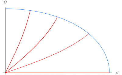
Figure 1: Projection of some null geodesics to the $(\rho,\theta)$ plane for the near horizon BMPV solution at $j=1.1$. The quarter ellipse is the boundary of the chronologically safe region, which coincides with the optical horizon $\aleph$.

3.5 Global Issues and NUT Singularity

The metric (3.1) interpreted as in this section has a problem when one considers it globally. As the coordinate $\varphi$ is periodic with period $2\pi$, and the length of the coordinate vector $\partial_{\varphi}$ vanishes at $\theta=0,\pi$, there are potential singularities at these loci. With the metric as written in (3.1) there is no singularity at $\theta=0$, because $\|\partial_{\varphi}\|\sim\theta R$. However at $\theta=\pi$ the norm of $\partial_{\varphi}$ does not vanish, and therefore there will be a singularity. This singularity is of Taub-NUT type. Indeed, forgetting about the hyperbolic plane, we have exactly the angular part of the Lorentzian Taub-NUT spacetime. It is well known [46] that the singularity at $\theta=\pi$ can be removed if one takes the coordinate $\tau$ periodic with period given by $4\pi\sqrt{j^{2}-1}R$ (the NUT charge). Indeed, replacing $\tau$ by $\tau^{\prime}=\tau-2\sqrt{j^{2}-1}R\varphi$ leads to good local coordinates near $\theta=\pi$. Note that this coordinate transformation is only allowed if $\tau$ has the correct periodicity.

This traditional point of view leads to an immediate problem with the proposal of holographic chronology protection of [1]. Since $\partial_{\tau}$ generates a timelike geodesic, if we make $\tau$ periodic, the induced metric on the holographic screen will have CTCs.

However, one can take a different point of view, which also interplays nicely with the holographic chronology protection. We notice that if we keep the NUT singularity at $\theta=\pi$, the holographic screen enclosing the observer at the origin is still causal and nonsingular. Indeed, the point $\theta=\pi$ lies strictly outside the chronologically safe region. Taking the point of view of [1], the CTCs as well as the singularities should not affect the holographic description of the physics accessible to our observer. We stress that this is quite a strong statement, since there is no event horizon surrounding the singularity. Hence, classically there are still causal paths connecting the observer to the singularity. A more palatable option is that these metrics only show up in a finite region of spacetime, and are patched to exterior metrics without CTCs, as in [16].

4 CTCs and Optical Horizons in Axisymmetric Spaces

In the last section we saw that for the overrotating near horizon BMPV metric, the optical horizon is coincident with the boundary of the chronologically safe region. In other words, the observer has no access through geodesic motion to the region where CTCs centered around him appear.

In this section we will discuss to which extent this feature is present in more general stationary axisymmetric space-times, in an arbitrary number of planes.

4.1 Axisymmetric Metrics

We consider a metric which is stationary and in addition is rotationally symmetric. More concretely, we will have a time coordinate $t$ and angular coordinates $\phi^{i}$, such that the vectors $\partial_{t}$ and $\partial_{\phi^{i}}$ are Killing. Furthermore we have several “radial” coordinates $\rho^{a}$. Our ansatz for the metric will be

$$ds^{2}=-k^{2}\Bigl{(}dt+A_{i}(d\phi^{i}+C^{i}_{a}\,d\rho^{a})+B_{a}\,d\rho^{a}\Bigr{)}^{2}+g_{ij}(d\phi^{i}+C^{i}_{a}\,d\rho^{a})(d\phi^{j}+C^{j}_{b}\,d\rho^{b})+h_{ab}\,d\rho^{a}\,d\rho^{b}\,,$$ (4.1)

where all functions may depend on the coordinates $\rho^{a}$. $k$, $g_{ij}$ and $h_{ab}$ are positive definite. Furthermore we assume the metric to be nonsingular. More precisely, we will assume that, after an appropriate coordinate transformation for $\rho$, near the origin $\rho=0$ $k$ is of order one, $g_{ij}$ is of order $\rho^{2}$ and $A_{i}$ is of order smaller than $\rho$. Note that not all $\rho^{a}$ have to be radial coordinates. However we will assume that the metric restricted to the $\rho$ plane is always Euclidean. This means that the $B_{a}$ should be bounded with respect to the metric $h_{ab}$.

Metrics of this form include the Van Stockum solution [47], the overrotating supertube solution [28], and many $(2n+1)$-dimensional Gödel universes formed by “rotation” in products of hyperbolic, spherical, or flat planes [43, 15]. The different values for the metric $g_{ij}$ and the connection $A_{i}$ for these situations are given schematically in Table 2.

plane	$g$	$A$
flat	$\rho^{2}$	$\frac{1}{2}a\rho^{2}$
hyperbolic	$\sinh^{2}\rho$	$2a\sinh^{2}\frac{\rho}{2}$
sphere	$\sin^{2}\rho$	$2a\sin^{2}\frac{\rho}{2}$

Table 2: Metrics and connections on Gödel planes.

4.2 Closed Timelike Curves

Let us first identify the closed timelike curves. We will be interested in an observer located at the origin $\rho=0$. By our assumption closed timelike curves necessarily involve nontrivial motion in the $\phi$ plane. Therefore to find the chronologically safe region we should consider the metric on the $\phi$ plane. As argued in the last section, in any region in the $\rho$ plane where this metric is positive definite there can not be a CTC.

The metric on the $\phi$ plane is given by

$$g_{(\phi)}=(g_{ij}-k^{2}A_{i}A_{j})\,d\phi^{i}\,d\phi^{j}\,.$$ (4.2)

Because there is at most one time direction, the signature of this metric is completely determined by the sign of its determinant. This determinant is easily calculated,

$$\det g_{(\phi)}=(1-k^{2}g^{ij}A_{i}A_{j})\det g_{ij}\,.$$ (4.3)

We conclude that in the region determined by

$$k^{2}g^{ij}A_{i}A_{j}<1\,,$$ (4.4)

the metric on the $\phi$ plane is Euclidean and therefore does not contain any closed timelike curve. Notice that this region encloses the observer at the origin. Moreover, strictly outside this region, where the determinant is negative, one finds closed curves moving only in the $\phi$ plane which are everywhere timelike.

4.3 Geodesics

We will now analyze the geodesics for a metric of the form (4.1). The symmetries generated by the Killing vectors $\partial_{t}$ and $\partial_{\phi^{i}}$ give rise to conserved charges

$$E = k^{2}(\dot{t}+A_{i}(\dot{\phi}^{i}+C^{i}_{a}\dot{\rho}^{a})+B_{a}\dot{\rho}^{a})\,,$$ (4.5)

$$J_{i} = g_{ij}(\dot{\phi}^{j}+C^{j}_{a}\dot{\rho}^{a})-EA_{i}.$$ (4.6)

The momenta conjugate to the coordinates $\rho^{a}$ are given by

$$\pi_{a}=h_{ab}\dot{\rho}^{b}+C^{i}_{a}J_{i}-EB_{a}\,.$$ (4.7)

The Hamiltonian for the geodesic flow, $H=g^{\mu\nu}\pi_{\mu}\pi_{\nu}$, is in this case

$$H = -\frac{E^{2}}{2k^{2}}+\frac{1}{2}g^{ij}(J_{i}+EA_{i})(J_{j}+EA_{j})$$ (4.8)

$$+\frac{1}{2}h^{ab}(\pi_{a}+EB_{a}-J_{i}C^{i}_{a})(\pi_{b}+EB_{b}-J_{j}C^{j}_{b})\,.$$

We are interested in the null geodesics that pass through the worldline of the observer at the origin. We find from the form of the momenta $J_{i}$ and our assumptions on the metric components near $\rho=0$ that such geodesics must necessarily have $J_{i}=0$. This is natural, as they can not have angular momenta when they pass the origin. For these geodesics the form of the Hamiltonian $H$, simplifies considerably. Furthermore, for null geodesics the Hamiltonian constraint reads $H=0$, so all in all,

$$H=-\frac{E^{2}}{2k^{2}}(1-k^{2}g^{ij}A_{i}A_{j})+\frac{1}{2}h^{ab}(\pi_{a}+EB_{a})(\pi_{b}+EB_{b})=0\,.$$ (4.9)

We recognize in the first term, the effective potential, the same factor we saw in the analysis of the closed timelike curves. Because the last term is non-negative, we conclude that any geodesic passing through $\rho=0$ will remain in the chronologically safe region (4.4).

4.4 Generic Location of the Optical Horizon

We now want to compare the location of the optical horizon with the boundary of the chronologically safe region. We just showed that for these spacetimes, the optical horizon never reaches beyond the chronologically safe region. In what follows we will argue that typically the optical horizon coincides with the boundary of the chronologically safe region (in a sense to be clarified below), although we will also show that in some cases the optical horizon is strictly inside such region.

Let us, as a simple example, consider a $(2n+1)$-dimensional spacetime which is a set of $n$ flat Gödel planes, i.e., the metric is given by

$$ds^{2}=-\Bigl{(}dt+\sum_{i=1}^{n}\omega_{i}r_{i}^{2}d\phi_{i}\Bigr{)}^{2}+\sum_{i=1}^{n}(r_{i}^{2}d\phi_{i}^{2}+dr_{i}^{2})\,,$$ (4.10)

with $\omega_{i}$ some constants. The chronologically safe region is determined by the ball

$$\sum_{i=1}^{n}\omega_{i}^{2}r_{i}^{2}<1\,.$$ (4.11)

The null geodesics passing through $r=0$ for this spacetime are easily found using the discussion above. Setting $E=1$, they are given by

$$r_{i}(\lambda)=R_{i}\sin\omega_{i}\lambda\,,$$ (4.12)

with

$$\sum_{i=1}^{n}\omega_{i}^{2}R_{i}^{2}=1\,.$$ (4.13)

The angles $\phi^{i}$ will depend linearly on $\lambda$. It follows from the previous equations that the null geodesics never escape the chronologically safe region. Furthermore, we recognize the projection of the null geodesics as a Lissajous figure, which will be a closed curve iff all the ratios $w_{i}/w_{j}$ are rational.

We now discuss in turn the possible cases, depending on the values of $w_{i}/w_{j}$. Assume first that all these ratios are rational. Then, we can still distinguish two possibilities: either all the ratios are given by fractions of odd integers, or they are not. In the first case,

$$\frac{w_{i}}{w_{j}}=\frac{2n_{i}+1}{2n_{j}+1}\,,\qquad\forall\;i,j\,,\qquad n_{i}\in\mathbb{Z}\,,$$ (4.14)

it follows that there is a value of $\lambda$ for which all $r_{i}(\lambda)=R_{i}$, (or equivalently, all $\dot{r}_{i}=0$ simultaneously), and the projection of the null geodesic manages to touch the boundary of the chronologically safe region, before focusing back towards the origin. We conclude that in this case the optical horizon coincides with the boundary of the chronologically safe region.

Although we carried out this analysis for metrics with flat Gödel planes, it is true more generally. For instance, for the near horizon BMPV metric discussed in the last section, we already showed that the frequencies of rotation in the hyperbolic plane and the sphere are equal, for the generic null geodesic. This is reflected in Figure 1, where we see that for the near horizon BMPV metric, the projection of the geodesics to the $\rho$ plane collapses, that is it follows exactly the same path going away from the origin as when it comes back. This finetuning of frequencies is actually common among the supersymmetric solutions discussed in the literature [15].

Next, we consider the case when the ratios $w_{i}/w_{j}$ are still all rational, but now some are given by a fraction involving an even and an odd integer

$$\frac{w_{i}}{w_{j}}=\frac{2n_{i}}{2n_{j}+1}\,,\qquad\mbox{for some }i,j\,,\qquad n_{i}\in\mathbb{Z}\,.$$ (4.15)

In this situation, the null geodesics can reach the boundary of the chronologically safe region only if they don’t have momentum in the $r_{i}$ directions associated to an even integer, so in general the optical horizon touches the boundary chronologically safe region, but does not coincide with it.

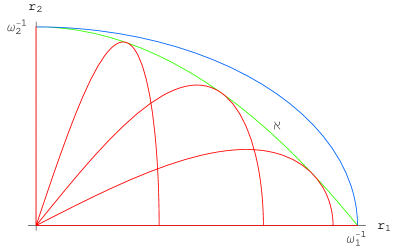
Figure 2: Projection of some null geodesics to the $r_{1},r_{2}$-plane for the flat Gödel solution in 5 dimensions for $\omega_{2}=2\omega_{1}$. The outer curve is the boundary of the chronologically safe region, the inner curve $\aleph$ is the optical horizon, which is the hull of the projected null geodesics through the origin.

Perhaps an example will clarify this. Consider the metric for two flat Gödel planes with $\omega_{2}/\omega_{1}=2$. The projections of some null geodesics to the $(r_{1},r_{2})$ plane passing through the origin are drawn in Figure 2. The figure already suggests that, as we just discussed, these null geodesics will not all come close to the boundary of the safe region, indicated in the figure by the enclosing quarter ellipse. In this simple example we can do even better, and find explicitly the optical horizon. To do so, notice that

$$1-\omega_{1}^{2}r_{1}^{2}(\lambda)-2\omega_{1}r_{2}(\lambda) = 1-\omega_{1}^{2}R_{1}^{2}\sin^{2}\omega_{1}\lambda-2\omega_{1}R_{2}\sin 2\omega_{1}\lambda$$

$$= (2\omega_{1}R_{2}\sin\omega_{1}\lambda-\cos\omega_{1}\lambda)^{2}\geq 0\,,$$

and moreover the bound is saturated for $\cot\lambda=2\omega_{1}R_{2}$. This implies that the optical horizon $\aleph$ is given by the surface at

$$\omega_{1}^{2}r_{1}^{2}+2\omega_{1}r_{2}=1\,,$$ (4.16)

which lies strictly inside the chronologically safe region, given by (4.11).

Finally, let’s consider the generic case, when some or all of the ratios $w_{i}/w_{j}$ are not rational. Now the projections of the geodesics are no longer closed curves. Such a situation is sketched in Figure 3. As suggested by the figure, the geodesics will densely fill a rectangular region bounded by $r_{i}=R_{i}$. A corner of this rectangle will exactly lie on the boundary of the chronologically safe region. So even though the geodesics will never reach this boundary, they will come arbitrarily close to it. This can be argued more precisely from the form of the solutions of the geodesics in the $r$ plane. Indeed, when the $\omega_{i}$ have non-rational quotients, we can make the $\dot{r}_{i}(\lambda)$ simultaneously arbitrarily small, which is equivalent, according to (4.9), to moving arbitrarily close to the boundary of the safe region.

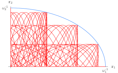
Figure 3: Projection of some null geodesics to the $r_{1},r_{2}$-plane for the flat Gödel solution in 5 dimensions for $\omega_{2}/\omega_{1}=2.61799\ldots$. The outer curve is the boundary of the chronologically safe region, as well as the optical horizon $\aleph$. The geodesics are followed only for a finite time; a full null geodesic would densely fill a rectangular region.

For more general metrics of the form (4.1), we can argue that generically the null geodesics will come arbitrarily close to the boundary of the safe region. We saw that the motion of the geodesics in the $\rho$ plane was governed by a Hamiltonian flow with total zero energy. Furthermore, the chronologically safe region is a cavity around $\rho=0$ bounded by the hypersurface of zero effective potential. We can now invoke the Poincaré recurrence theorem. It states in particular that for generic parameters in the potential, any integral curve of this motion will densely fill the phase space region of constant energy. Here we assumed that the cavity is in fact compact. This part of the phase space will project to the whole cavity inside zero effective potential. This implies that any null geodesic will come arbitrarily close to the boundary of the safe region, and therefore the optical horizon will coincide with this boundary.

To summarize, for metrics with flat Gödel planes, the optical horizon coincides with the boundary of the chronologically safe region, unless some frequencies satisfy $w_{i}/w_{j}=2n_{i}/(2n_{j}+1)$.

Note that in the example of flat Gödel planes in this section the individual geodesics did not fill the whole cavity, but rather a rectangular region fitting just inside it. Of course the form of the metric was certainly not generic, as the radial dependence of the various functions was taken to be particularly simple.

5 Discussion and Conclusions

We have studied in detail an example of a spacetime homogeneous 5d supergravity solution with closed timelike curves, the near horizon of an overrotating BMPV black hole. As discussed in previous sections, this solution can be thought of as two Gödel type planes (one hyperbolic, one spherical) related to the 4d Gödel type solutions presented in [43] and studied in [23, 24]. As a result, the qualitative pattern of the regions with CTCs and optical horizon is quite similar. Some of our results, like the relation between null geodesics and optical horizon, are a direct consequence of the spacetime homogeneity of the solution, so we expect them to be true in arbitrary spacetime homogeneous solutions.

As a welcome spin-off of our study, we have brought to a full conclusion the classification of maximally supersymmetric solutions in five dimensional minimal supergravity. Namely, we found that the three unidentified solutions of [13] belong to the NH-BMPV family, so the five solutions listed in the introduction are the full set of maximally supersymmetric backgrounds of this theory. Furthermore we showed explicitly how they arise from reductions of $AdS_{3}\times S^{3}$, and how the different reductions determine their causal structures. Finally, we also elucidated the relation between $AdS_{3}\times S^{2}$ and the NH-BMPV family, arguing than the former does not belong to the NH-BMPV family.

We also considered more general axisymmetric metrics with closed timelike curves, not necessarily homogeneous. Within the class of metrics discussed, we showed that the null geodesics passing through the origin never escape the chronologically safe region. We expect this to be true in much more generality, and it would be interesting to generalize our proof. In particular, our arguments show that the observation of [1] that holographic screens are inside the chronologically safe region for Gödel type solutions applies to a much wider class of metrics.

The physical relevance of such observation depends of course on the possibility of realizing such metrics. Within the context of string theory, probe computations [28, 29, 16] suggest in particular cases that ten dimensional solutions with closed timelike curves can’t be built starting from flat space. It would be important to understand the generality of this assertion.

Acknowlegements

We would like to thank José Figueroa-O’Farrill, Veronika Hubeny, Patrick Meessen and Tomás Ortín, for useful conversations. BF would also like to thank the ITP at Stanford University and the KITP at UCSB for hospitality. The work of BF was supported by a Marie Curie Fellowship. The work of E.L.-T. was supported in part by by the Spanish grant BFM2003-01090. The work of C.H. was partly supported by a Koshland Scholarship. In addition, this work was supported by the Israel-U.S. Binational Science Foundation, by the ISF Centers of Excellence program, by the European network HPRN-CT-2000-00122 and by Minerva.

Appendix A Hopf Fibrations of $S^{3}$ and $AdS_{3}$

In this appendix we will write down the explicit Hopf fibrations of $S^{3}$ and especially $AdS_{3}$.

A.1 Hopf Fibration of $S^{3}$

We start with the well known Hopf fibration of $S^{3}$, identified with the group manifold $\mathop{\kern 0.0pt\mathrm{SU}}\nolimits(2)$. We use the anti-Hermitian basis for $\mathop{\kern 0.0pt\mathit{su}}\nolimits(2)$ given by $\hat{\tau}^{a}=\frac{i}{2}\sigma^{a}$, where $\sigma^{a}$ are the standard Pauli spin matrices. We then parametrize the group elements $g\in\mathop{\kern 0.0pt\mathrm{SU}}\nolimits(2)$ as

$$g=\mathop{\kern 0.0pt\mathrm{e}}\nolimits^{\phi\hat{\tau}^{3}}\mathop{\kern 0.0pt\mathrm{e}}\nolimits^{\theta\hat{\tau}^{2}}\mathop{\kern 0.0pt\mathrm{e}}\nolimits^{\psi\hat{\tau}^{3}}\,.$$ (A.1)

The left-invariant one-forms $\omega^{a}$ can be found from

$$g^{\raise 0.45206pt\hbox{${\scriptscriptstyle-}$}\kern-0.35002pt1}dg=\omega^{a}\hat{\tau}^{a}\,.$$ (A.2)

We find

$$\left\{\begin{array}[]{r@{\;}c@{\;}l}\omega^{1}&=&-\sin\psi\,d\theta+\cos\psi\sin\theta\,d\phi\,,\\ \omega^{2}&=&\cos\psi\,d\theta+\sin\psi\sin\theta\,d\phi\,,\\ \omega^{3}&=&d\psi+\cos\theta\,d\phi\,.\end{array}\right.$$ (A.3)

The metric is given by $-\mathop{\kern 0.0pt\mathrm{tr}}\nolimits(g^{\raise 0.45206pt\hbox{${\scriptscriptstyle-}$}\kern-0.35002pt1}dg)^{2}=\frac{1}{4}\sum_{a}(\omega^{a})^{2}$, where $\mathop{\kern 0.0pt\mathrm{tr}}\nolimits$ is a trace normalized such that $\mathop{\kern 0.0pt\mathrm{tr}}\nolimits\hbox{1\kern-2.5ptl}=1$. This leads to the metric

$$d\Omega_{(3)}^{2}=\frac{1}{4}d\theta^{2}+\frac{1}{4}\sin^{2}\theta\;d\phi^{2}+\frac{1}{4}(d\psi+\cos\theta\;d\phi)^{2}\,.$$ (A.4)

The Killing vectors for the left action of $\mathop{\kern 0.0pt\mathrm{SU}}\nolimits(2)$ are given by

$$\left\{\begin{array}[]{r@{\;}c@{\;}l}\xi^{L}_{1}&=&\displaystyle\sin\phi\;\partial_{\theta}+\cos\phi\cot\theta\;\partial_{\phi}-\cos\phi\mathop{\kern 0.0pt\mathrm{cosec}}\nolimits\theta\;\partial_{\psi}\,,\\ \xi^{L}_{2}&=&\displaystyle\cos\phi\;\partial_{\theta}-\sin\phi\cot\theta\;\partial_{\phi}+\sin\phi\mathop{\kern 0.0pt\mathrm{cosec}}\nolimits\theta\;\partial_{\psi}\,,\\ \xi^{L}_{3}&=&\partial_{\phi}\,,\end{array}\right.$$ (A.5)

while the right action of $\mathop{\kern 0.0pt\mathrm{SU}}\nolimits(2)$ is generated by the Killing vectors

$$\left\{\begin{array}[]{r@{\;}c@{\;}l}\xi^{R}_{1}&=&\displaystyle-\sin\psi\;\partial_{\theta}-\cos\psi\cot\theta\;\partial_{\psi}+\cos\psi\mathop{\kern 0.0pt\mathrm{cosec}}\nolimits\theta\;\partial_{\phi}\,,\\ \xi^{R}_{2}&=&\displaystyle\cos\psi\;\partial_{\theta}-\sin\psi\cot\theta\;\partial_{\psi}+\sin\phi\mathop{\kern 0.0pt\mathrm{cosec}}\nolimits\theta\;\partial_{\phi}\,,\\ \xi^{R}_{3}&=&\partial_{\psi}\,.\end{array}\right.$$ (A.6)

These Killing vectors are normalized such that $\xi^{R}_{i}\cdot\omega_{L}^{j}=\xi^{L}_{i}\cdot\omega_{R}^{j}=\delta_{i}^{j}$.

A.2 Spacelike Hopf Fibration of $AdS_{3}$

For $AdS_{3}$ we can write down Hopf fibrations very similar as for the one over $S^{3}$. For this we identify $AdS_{3}$ with $\widetilde{\mathop{\kern 0.0pt\mathrm{SL}}\nolimits}(2)$. We will use the basis of $\mathop{\kern 0.0pt\mathit{sl}}\nolimits(2)$ given by the real matrices $\hat{\tau}^{1}=\frac{1}{2}\sigma^{1}$, $\hat{\tau}^{2}=\frac{i}{2}\sigma^{2}$, and $\hat{\tau}^{3}=\frac{1}{2}\sigma^{3}$.

In the $AdS_{3}$ case there are essentially three different Hopf fibrations, depending on whether the Hopf fiber is in a spacelike, timelike, or lightlike direction. We will first study the spacelike case.

For the spacelike Hopf fibration we take the following parametrization of $g\in\mathop{\kern 0.0pt\mathrm{SL}}\nolimits(2)$,

$$g=\mathop{\kern 0.0pt\mathrm{e}}\nolimits^{\tau\hat{\tau}^{2}}\mathop{\kern 0.0pt\mathrm{e}}\nolimits^{\rho\hat{\tau}^{1}}\mathop{\kern 0.0pt\mathrm{e}}\nolimits^{\psi\hat{\tau}^{3}}.$$ (A.7)

The Hopf fibration is given by the right action of the hyperbolic one-parameter subgroup generated by $\hat{\tau}^{3}$. The left-invariant one-forms $\omega^{a}$ are determined in the same way as for $S^{3}$, and in this case are given by

$$\left\{\begin{array}[]{r@{\;}c@{\;}l}\omega^{1}&=&\cosh\psi\,d\rho-\sinh\psi\cosh\rho\,d\tau\,,\\ \omega^{2}&=&-\sinh\psi\,d\rho+\cosh\psi\cosh\rho\,d\tau\,,\\ \omega^{3}&=&d\psi+\sinh\rho\,d\tau\,.\end{array}\right.$$ (A.8)

The metric will now be given by $4\mathop{\kern 0.0pt\mathrm{tr}}\nolimits(g^{\raise 0.45206pt\hbox{${\scriptscriptstyle-}$}\kern-0.35002pt1}dg)^{2}=\sum_{a}(\omega^{a})^{2}$. It can then be written

$$ds^{2}=-\cosh^{2}\rho\,d\tau^{2}+d\rho^{2}+(d\psi+\sinh\rho\,d\tau)^{2}\,.$$ (A.9)

A.3 Timelike Hopf Fibration of $AdS_{3}$

For the timelike Hopf fibration we take the following parametrization of $\mathop{\kern 0.0pt\mathrm{SL}}\nolimits(2)$,

$$g=\mathop{\kern 0.0pt\mathrm{e}}\nolimits^{\tau\hat{\tau}^{3}}\mathop{\kern 0.0pt\mathrm{e}}\nolimits^{\rho\hat{\tau}^{1}}\mathop{\kern 0.0pt\mathrm{e}}\nolimits^{\psi\hat{\tau}^{2}}.$$ (A.10)

The Hopf fibration is given by the right action of the hyperbolic one-parameter subgroup generated by $\hat{\tau}^{2}$. The left-invariant one-forms $\omega^{a}$ are given by

$$\left\{\begin{array}[]{r@{\;}c@{\;}l}\omega^{1}&=&\cos\psi\,d\rho+\sin\psi\cosh\rho\,d\tau\,,\\ \omega^{2}&=&d\psi+\sinh\rho\,d\tau\,,\\ \omega^{3}&=&-\sin\psi\,d\rho+\cos\psi\cosh\rho\,d\tau\,.\end{array}\right.$$ (A.11)

The metric can then be written

$$ds^{2}=\cosh^{2}\rho\,d\tau^{2}+d\rho^{2}-(d\psi+\sinh\rho\,d\tau)^{2}.$$ (A.12)

A.4 Lightlike Hopf Fibration of $AdS_{3}$

For the lightlike Hopf fibration we need yet another parametrization of $\mathop{\kern 0.0pt\mathrm{SL}}\nolimits(2)$. Let us introduce parabolic generators $\hat{\tau}^{\pm}=\hat{\tau}^{1}\pm\hat{\tau}^{2}$ of $\mathop{\kern 0.0pt\mathit{sl}}\nolimits(2)$. We parametrize $\mathop{\kern 0.0pt\mathrm{SL}}\nolimits(2)$ by

$$g=\mathop{\kern 0.0pt\mathrm{e}}\nolimits^{\tau\hat{\tau}^{-}}\mathop{\kern 0.0pt\mathrm{e}}\nolimits^{\rho\hat{\tau}^{3}}\mathop{\kern 0.0pt\mathrm{e}}\nolimits^{\psi\hat{\tau}^{+}}.$$ (A.13)

The Hopf fibration is given by the right action of the parabolic one-parameter subgroup generated by $\hat{\tau}^{+}$. The left-invariant one-forms $\omega^{a}$ are given by

$$\left\{\begin{array}[]{r@{\;}c@{\;}l}\omega^{+}&=&d\psi+\psi\,d\rho-\psi^{2}\mathop{\kern 0.0pt\mathrm{e}}\nolimits^{\rho}d\tau\,,\\ \omega^{-}&=&\mathop{\kern 0.0pt\mathrm{e}}\nolimits^{\rho}d\tau\,,\\ \omega^{3}&=&d\rho-2\psi\mathop{\kern 0.0pt\mathrm{e}}\nolimits^{\rho}d\tau\,.\end{array}\right.$$ (A.14)

Therefore the metric can be written

$$ds^{2}=(\omega^{3})^{2}+4\omega^{+}\omega^{-}=d\rho^{2}+4\mathop{\kern 0.0pt\mathrm{e}}\nolimits^{\rho}d\tau\,d\psi\,.$$ (A.15)

A.5 Alternative Hopf Fibrations of $AdS_{3}$

there are alternative parametrizations of the group $\mathop{\kern 0.0pt\mathrm{SL}}\nolimits(2)$, which are actually somewhat closer to the Hopf fibration of the sphere. For the spacelike Hopf fibration we write

$$g=\mathop{\kern 0.0pt\mathrm{e}}\nolimits^{\tau\hat{\tau}^{3}}\mathop{\kern 0.0pt\mathrm{e}}\nolimits^{\rho\hat{\tau}^{1}}\mathop{\kern 0.0pt\mathrm{e}}\nolimits^{\psi\hat{\tau}^{3}}\,.$$ (A.16)

The Hopf fibration can be seen as the right action by the elliptic 1-parameter subgroup of $\widetilde{\mathop{\kern 0.0pt\mathrm{SL}}\nolimits}(2)$ generated by $\hat{\tau}^{3}$. The left-invariant one-forms $\omega^{a}$ are given by

$$\left\{\begin{array}[]{r@{\;}c@{\;}l}\omega^{1}&=&\cosh\psi\,d\rho-\sinh\psi\sinh\rho\,d\tau\,,\\ \omega^{2}&=&-\sinh\psi\,d\rho+\cosh\psi\sinh\rho\,d\tau\,,\\ \omega^{3}&=&d\psi+\cosh\rho\,d\tau\,.\end{array}\right.$$ (A.17)

The metric in this parametrization becomes

$$ds^{2}=-\sinh^{2}\rho\,d\tau^{2}+d\rho^{2}+(d\psi+\cosh\rho\,d\tau)^{2}.$$ (A.18)

For the timelike Hopf fibration we take the parametrization

$$g=\mathop{\kern 0.0pt\mathrm{e}}\nolimits^{\tau\hat{\tau}^{2}}\mathop{\kern 0.0pt\mathrm{e}}\nolimits^{\rho\hat{\tau}^{1}}\mathop{\kern 0.0pt\mathrm{e}}\nolimits^{\psi\hat{\tau}^{2}}.$$ (A.19)

This leads to left-invariant one-forms $\omega^{a}$ given by

$$\left\{\begin{array}[]{r@{\;}c@{\;}l}\omega^{1}&=&\cos\psi\,d\rho+\sin\psi\sinh\rho\,d\tau\,,\\ \omega^{2}&=&d\psi+\cosh\rho\,d\tau\,,\\ \omega^{3}&=&-\sin\psi\,d\rho+\cos\psi\sinh\rho\,d\tau\,.\end{array}\right.$$ (A.20)

The metric in this parametrization becomes

$$ds^{2}=\sinh^{2}\rho\,d\tau^{2}+d\rho^{2}-(d\psi+\cosh\rho\,d\tau)^{2}\,.$$ (A.21)

Appendix B $AdS_{3}$ Metrics in Poincaré Coordinates

The metric for $AdS_{3}$ on a Poincaré patch can be written in the form

$$ds^{2}_{AdS_{3}}=\frac{dr^{2}}{r^{2}}+2r\,dt\,du+\alpha\;du^{2}\,.$$ (B.1)

This is a valid $AdS_{3}$ metric for any value of $\alpha$, in particular, after a rescaling, it can be chosen as $\alpha=\pm 1$ or $\alpha=0$. We will show below that these three cases correspond to the three different Hopf fibrations of $AdS_{3}$, which along the way establishes them as metrics on $AdS_{3}$. For $\alpha=0$, the relation with the lightlike Hopf fibration (A.15) is obvious. For $\alpha=\pm 1$ we can write this metric in the form

$$ds^{2}=\frac{dr^{2}}{r^{2}}-\alpha r^{2}dt^{2}+\alpha(du+rdt)^{2}\,,$$ (B.2)

where we rescaled $t\to\alpha t$ for convenience.

B.1 Coordinate Transformations in the Spacelike Case

First consider the Poincaré metric (B.2) for $\alpha=1$. Then consider the coordinate transformation

$$\left\{\begin{array}[]{r@{\;}c@{\;}l}r&=&\sinh\rho+\cosh\rho\cos\tau\,,\\ rt&=&\cosh\rho\sin\tau\,,\\ u&=&\displaystyle\psi-2\mathop{\kern 0.0pt\mathrm{arctanh}}\nolimits\Bigl{(}\mathop{\kern 0.0pt\mathrm{e}}\nolimits^{-\rho}\tan\frac{\tau}{2}\Bigr{)}\,.\end{array}\right.$$ (B.3)

From these transformations we derive

$$\frac{dr^{2}}{r^{2}}-r^{2}dt^{2}=d\rho^{2}-\cosh^{2}\rho\;d\tau^{2}\,,\qquad du+rdt=d\psi+\sinh\rho\;d\tau\,.$$ (B.4)

Using this, we find that the metric (B.2) for $\alpha=1$ becomes the metric (A.9) in global coordinates. Because we have established the separate identities above, we can also apply this coordinate transformation to the five dimensional metric for $j<1$.

B.2 Coordinate Transformations in the Timelike Case

Next we consider the Poincaré metric (B.2) for $\alpha=-1$. We take the coordinate transformation

$$\left\{\begin{array}[]{r@{\;}c@{\;}l}r&=&\sinh\rho+\cosh\rho\cosh\tau\,,\\ rt&=&\cosh\rho\sinh\tau\,,\\ u&=&\displaystyle\psi-2\arctan\Bigl{(}\mathop{\kern 0.0pt\mathrm{e}}\nolimits^{-\rho}\tanh\frac{\tau}{2}\Bigr{)}\,.\end{array}\right.$$ (B.5)

From these transformations we derive

$$\frac{dr^{2}}{r^{2}}+r^{2}dt^{2}=d\rho^{2}+\cosh^{2}\rho\;d\tau^{2}\,,\qquad du+rdt=d\psi+\sinh\rho\;d\tau\,.$$ (B.6)

Using these relations we find that (B.2) for $\alpha=-1$ becomes the metric (A.12) in global coordinates. Again these coordinate transformations can be applied to the five dimensional metric for $j>1$.

B.3 Alternative Coordinate Transformations in the Spacelike Case

We can also relate the Poincaré metrics to the alternative Hopf fibrations. First consider the Poincaré metric (B.2) for $\alpha=1$. The coordinate transformation we consider is

$$\left\{\begin{array}[]{r@{\;}c@{\;}l}r&=&\cosh\rho+\sinh\rho\cosh\tau\,,\\ rt&=&\sinh\rho\sinh\tau\,,\\ u&=&\displaystyle\psi+2\mathop{\kern 0.0pt\mathrm{arctanh}}\nolimits\Bigl{(}\mathop{\kern 0.0pt\mathrm{e}}\nolimits^{-\rho}\tanh\frac{\tau}{2}\Bigr{)}\,.\end{array}\right.$$ (B.7)

From these transformations we derive

$$\frac{dr^{2}}{r^{2}}-r^{2}dt^{2}=d\rho^{2}-\sinh^{2}\rho\;d\tau^{2}\,,\qquad du+rdt=d\psi+\cosh\rho\;d\tau\,.$$ (B.8)

Hence the metric (B.2) for $\alpha=1$ becomes the metric (A.18) in global coordinates.

B.4 Alternative Coordinate Transformations in the Timelike Case

Next consider the Poincaré metric (B.2) with $\alpha=-1$. We consider the coordinate transformation

$$\left\{\begin{array}[]{r@{\;}c@{\;}l}r&=&\cosh\rho+\sinh\rho\cos\tau\,,\\ rt&=&\sinh\rho\sin\tau\,,\\ u&=&\displaystyle\psi+2\arctan\Bigl{(}\mathop{\kern 0.0pt\mathrm{e}}\nolimits^{-\rho}\tan\frac{\tau}{2}\Bigr{)}\,.\end{array}\right.$$ (B.9)

From these transformations we derive

$$\frac{dr^{2}}{r^{2}}+r^{2}dt^{2}=d\rho^{2}+\sinh^{2}\rho\;d\tau^{2}\,,\qquad du+rdt=d\psi+\cosh\rho\;d\tau\,.$$ (B.10)

Hence (B.2) with $\alpha=-1$ becomes the metric (A.21) in global coordinates.

References

- [1] E. K. Boyda, S. Ganguli, P. Hořava and U. Varadarajan, Holographic protection of chronology in universes of the Goedel type, Phys. Rev. D67, 106003 (2003) [arXiv:hep-th/0212087].
- [2] J. Simón, The geometry of null rotation identifications, JHEP 0206, 001 (2002) [arXiv:hep-th/0203201].
- [3] H. Liu, G. Moore and N. Seiberg, Strings in a time-dependent orbifold, JHEP 0206, 045 (2002) [arXiv:hep-th/0204168]. Strings in time-dependent orbifolds, JHEP 0210, 031 (2002) [arXiv:hep-th/0206182].
- [4] L. Cornalba and M. S. Costa, A new cosmological scenario in string theory, Phys. Rev. D66, 066001 (2002) [arXiv:hep-th/0203031].
- [5] R. Biswas, E. Keski-Vakkuri, R. G. Leigh, S. Nowling and E. Sharpe, The taming of closed timelike curves, arXiv:hep-th/0304241.
- [6] S. Elitzur, A. Giveon, D. Kutasov and E. Rabinovici, From big bang to big crunch and beyond, JHEP 0206, 017 (2002) [arXiv:hep-th/0204189].
- [7] B. Craps, D. Kutasov and G. Rajesh, String propagation in the presence of cosmological singularities, JHEP 0206, 053 (2002) [arXiv:hep-th/0205101].
- [8] O. Aharony, M. Fabinger, G. T. Horowitz and E. Silverstein, Clean time-dependent string backgrounds from bubble baths, JHEP 0207, 007 (2002) [arXiv:hep-th/0204158].
- [9] A. Buchel, P. Langfelder and J. Walcher, On time-dependent backgrounds in supergravity and string theory, Phys. Rev. D67, 024011 (2003) [arXiv:hep-th/0207214].
- [10] J. Khoury, B. A. Ovrut, N. Seiberg, P. J. Steinhardt and N. Turok, From big crunch to big bang, Phys. Rev. D65, 086007 (2002) [arXiv:hep-th/0108187].
- [11] S. W. Hawking, The Chronology protection conjecture, Phys. Rev. D46, 603 (1992).
- [12] L. Maoz and J. Simón, Killing spectroscopy of closed timelike curves, arXiv:hep-th/0310255.
- [13] J. P. Gauntlett, J. B. Gutowski, C. M. Hull, S. Pakis and H. S. Reall, All supersymmetric solutions of minimal supergravity in five dimensions, Class. Quant. Grav. 20 (2003) 4587 [arXiv:hep-th/0209114].
- [14] J. C. Breckenridge, R. C. Myers, A. W. Peet and C. Vafa, D-branes and spinning black holes, Phys. Lett. B391 (1997) 93 [arXiv:hep-th/9602065].
- [15] T. Harmark and T. Takayanagi, Supersymmetric Goedel universes in string theory, Nucl. Phys. B662, 3 (2003) [arXiv:hep-th/0301206].
- [16] N. Drukker, B. Fiol and J. Simón, Goedel’s universe in a supertube shroud, arXiv:hep-th/0306057.
- [17] Y. Hikida and S. J. Rey, Can branes travel beyond CTC horizon in Goedel universe?, Nucl. Phys. B669, 57 (2003) [arXiv:hep-th/0306148].
- [18] D. Brecher, P. A. DeBoer, D. C. Page and M. Rozali, Closed timelike curves and holography in compact plane waves, JHEP 0310, 031 (2003) [arXiv:hep-th/0306190].
- [19] D. Brace, C. A. R. Herdeiro and S. Hirano, Classical and quantum strings in compactified pp-waves and Goedel type universes, arXiv:hep-th/0307265.
- [20] D. Brace, Closed geodesics on Goedel-type backgrounds, arXiv:hep-th/0308098.
- [21] H. Takayanagi, Boundary states for supertubes in flat spacetime and Goedel universe, JHEP 0312, 011 (2003) [arXiv:hep-th/0309135].
- [22] D. Brecher, U. H. Danielsson, J. P. Gregory and M. E. Olsson, Rotating black holes in a Goedel universe, JHEP 0311 (2003) 033 [arXiv:hep-th/0309058].
- [23] N. Drukker, B. Fiol and J. Simón, Goedel-type universes and the Landau problem, arXiv:hep-th/0309199.
- [24] D. Israël, Quantization of heterotic strings in a Goedel/anti de Sitter spacetime and chronology protection, arXiv:hep-th/0310158.
- [25] R. Bousso, “Holography in general space-times,” JHEP 9906, 028 (1999) [arXiv:hep-th/9906022]. The holographic principle for general backgrounds, Class. Quant. Grav. 17, 997 (2000) [arXiv:hep-th/9911002].
- [26] G. W. Gibbons and C. A. R. Herdeiro, Supersymmetric rotating black holes and causality violation, Class. Quant. Grav. 16, 3619 (1999) [arXiv:hep-th/9906098].
- [27] A. Chamseddine, J. Figueroa-O’Farrill and W. Sabra, Supergravity vacua and Lorentzian Lie groups, arXiv:hep-th/0306278.
- [28] R. Emparan, D. Mateos and P. K. Townsend, Supergravity supertubes, JHEP 0107 (2001) 011 [arXiv:hep-th/0106012].
- [29] L. Dyson, Chronology protection in string theory, arXiv:hep-th/0302052.
- [30] R. C. Myers and M. J. Perry, Black holes in higher dimensional space-times, Annals Phys. 172 (1986) 304.
- [31] G. T. Horowitz and A. Sen, Rotating black holes which saturate a Bogomol’nyi bound, Phys. Rev. D53 (1996) 808 [arXiv:hep-th/9509108].
- [32] A. H. Chamseddine, S. Ferrara, G. W. Gibbons and R. Kallosh, Enhancement of supersymmetry near 5d black hole horizon, Phys. Rev. D55 (1997) 3647 [arXiv:hep-th/9610155].
- [33] R. Kallosh, A. Rajaraman and W. K. Wong, Supersymmetric rotating black holes and attractors, Phys. Rev. D55 (1997) 3246 [arXiv:hep-th/9611094].
- [34] J. P. Gauntlett, R. C. Myers and P. K. Townsend, Black holes of D = 5 supergravity, Class. Quant. Grav. 16 (1999) 1 [arXiv:hep-th/9810204].
- [35] N. Alonso-Alberca, E. Lozano-Tellechea and T. Ortin, The near-horizon limit of the extreme rotating d = 5 black hole as a homogeneous spacetime, Class. Quant. Grav. 20 (2003) 423 [arXiv:hep-th/0209069].
- [36] G. W. Gibbons, G. T. Horowitz and P. K. Townsend, Higher dimensional resolution of dilatonic black hole singularities, Class. Quant. Grav. 12 (1995) 297 [arXiv:hep-th/9410073].
- [37] P. Meessen, A small note on PP-wave vacua in 6 and 5 dimensions, Phys. Rev. D65 (2002) 087501 [arXiv:hep-th/0111031].
- [38] L. F. Abbott and S. Deser, Stability of gravity with a cosmological constant, Nucl. Phys. B195 (1982) 76.
- [39] E. Lozano-Tellechea, P. Meessen and T. Ortin, On d = 4, 5, 6 vacua with 8 supercharges, Class. Quant. Grav. 19 (2002) 5921 [arXiv:hep-th/0206200].
- [40] J. B. Gutowski, D. Martelli and H. S. Reall, All supersymmetric solutions of minimal supergravity in six dimensions, Class. Quant. Grav. 20 (2003) 5049 [arXiv:hep-th/0306235].
- [41] C. A. R. Herdeiro, Spinning deformations of the D1-D5 system and a geometric resolution of closed timelike curves, Nucl. Phys. B665, 189 (2003) [arXiv:hep-th/0212002].
- [42] J. Figueroa-O’Farrill and J. Simón, Supersymmetric Kaluza-Klein reductions of M2 and M5 branes, Adv. Theor. Math. Phys. 6 (2003) 703 [arXiv:hep-th/0208107].
- [43] M. J. Rebouças and J. Tiomno, On the homogeneity of Riemannian space-times of Godel type, Phys. Rev. D28, 1251 (1983).
- [44] J. P. Gauntlett, R. C. Myers and P. K. Townsend, Supersymmetry of rotating branes, Phys. Rev. D59 (1999) 025001 [arXiv:hep-th/9809065].
- [45] R. Geroch and G. T. Horowitz, Global structure of spacetime, in General Relativity. An Einstein centenary survey, S.W. Hawking and W. Israel (eds.). Cambridge University Press (1979).
- [46] C. Misner, J. Math. Phys. 4 (1963), 924.
- [47] W. J. van Stockum, Gravitational field of a distribution of particles rotating about an axis of symmetry, Proc. Roy. S. Edin. 57 (1937) 135.