On the Boundary Entropy of One-dimensional Quantum Systems at Low Temperature

Abstract

The boundary $\beta$-function generates the renormalization group acting on the universality classes of one-dimensional quantum systems with boundary which are critical in the bulk but not critical at the boundary. We prove a gradient formula for the boundary $\beta$-function, expressing it as the gradient of the boundary entropy $s$ at fixed non-zero temperature. The gradient formula implies that $s$ decreases under renormalization except at critical points (where it stays constant). At a critical point, the number $\exp(s)$ is the “ground-state degeneracy,” $g$, of Affleck and Ludwig, so we have proved their long-standing conjecture that $g$ decreases under renormalization, from critical point to critical point. The gradient formula also implies that $s$ decreases with temperature except at critical points, where it is independent of temperature. The boundary thermodynamic energy $u$ then also decreases with temperature. It remains open whether the boundary entropy of a 1-d quantum system is always bounded below. If $s$ is bounded below, then $u$ is also bounded below.

I Introduction

The logarithm of the partition function $\ln Z=\ln\mathrm{Tr}\exp(-\beta H)$ for a one-dimensional quantum critical system with a boundary takes the universal formAffleck and Ludwig (1991) $(c\pi/6)(L/\beta)+\ln g$ where $H$ is the hamiltonian, $\beta=1/T$ the inverse temperature, $L\gg\beta$ is the length, $c$ is the numerical coefficient of the bulk conformal anomaly, and $g$ is the¡ “universal noninteger ground-state degeneracy” at the boundary (using natural units in which $\hbar=k=v=1$, $v$ being the velocity of “light”). This formula applies in the limit of large $L$. The number $g$ is an invariant of the universality class of the critical boundary condition. It was conjectured that $g$ decreases from critical point to critical point under renormalizationAffleck and Ludwig (1991, 1993).

For a 1-d quantum system that is critical in the bulk but is not critical at the boundary, the logarithm of the partition function at low temperature can be written in the form $\ln Z=(c\pi/6)(L/\beta)+\ln z_{L}$ and the boundary partion function $z$ can be defined as $\lim_{L\rightarrow\infty}z_{L}$. That is, the partition function takes the universal form

$$\ln Z=(c\pi/6)(L/\beta)+\ln z$$ (1)

up to corrections which vanish in the limit $L\rightarrow\infty$.

Quantum critical points occur at zero temperature. At temperature $T>0$, the correlation functions are of course not scale-invariant, but decay exponentially at distance scale $\beta=1/T$. Nevertheless, it is meaningful to talk of a bulk critical system at temperature $T>0$. The low energy degrees of freedom and their coupling constants can be identified in the $T=0$ critical system, which is described by a 1+1 dimensional quantum field theory. That quantum field theory, at temperature $T>0$, describes the quantum critical system at temperature $T$. It is possible to identify temperature-independent coupling constants within the critical system. These coupling constants can be held to their critical values when the temperature is above zero. Quantum critical phenomena are special in this respect. In generic critical phenomena, which have non-zero critical temperatures, the temperature is just one of the coupling constants.

Given that the bulk system is critical and that $L=\infty$, the only dimensionful parameter is the temperature $T$. The logarithm of the boundary partition function is thus a function $\ln z(\mu\beta)$ that depends only on the temperature, in units of $\mu$, where $\mu$ is a small temperature that sets the renormalization scale (or, equivalently, a small energy or inverse time or inverse distance). The total entropy then takes the universal form

$$S=(1-\beta\partial/\partial\beta)\ln Z=(c\pi/3)(L/\beta)+s(\mu\beta)$$ (2)

where $s(\mu\beta)=(1-\beta\partial/\partial\beta)\ln z$ is the boundary entropy. At a critical point, $s$ is equal to the constant $\ln g$.

We prove here a gradient formula

$$g_{ab}(\lambda)\beta^{b}(\lambda)=-\partial s/\partial\lambda^{a}$$ (3)

where the $\lambda^{a}$ form a complete set of boundary coupling constants, $g_{ab}(\lambda)$ is a certain metric on the space of all boundary conditions, and $\beta^{a}(\lambda)$ is the boundary $\beta$-function. It follows directly from the gradient formula that $\mu\partial s/\partial\mu=\beta^{a}\partial_{a}s=-g_{ab}\beta^{a}\beta^{b}$ so $s$ decreases under the renormalization group except where $\beta^{a}=0$, at the critical points. The gradient formula eliminates the possibility of esoteric asymptotic behavior under renormalization. Recurring trajectories such as limit cycles are excluded. The $g$-conjecture for the rg flows between critical points is a corollary of the gradient formula.

The gradient formula implies equally that the boundary entropy decreases with temperature, $\beta\partial s/\partial\beta=\mu\partial s/\partial\mu<0$. The total entropy $S$ obviously decreases with temperature, because $\partial S/\partial\beta=-\beta\langle(H-\langle H\rangle)^{2}\rangle$. However, the decrease of the bulk contribution $(\pi/3)(L/\beta)c$ masks the change in $s$, so it is not obvious that the boundary entropy by itself must decrease with temperature. The gradient formula implies that it does. It follows that the thermodynamic boundary energy also decreases with temperature, $\mu\beta\partial u/\partial\beta=\partial s/\partial\beta<0$.

Complete control over the possible behavior at asymptotically low temperature is still lacking, because we do not prove that $s$ is bounded below. If $s$ is bounded below, then the system must go to a critical point at zero temperature. Of course, the total entropy $S$ of any system is bounded below, as long as the system is of finite size. So, for any finite size $L$, $s_{L}=S-(c\pi/3)(L/\beta)$ is bounded below, as $T\rightarrow 0$. However, the lower bound can descend without limit as $L\rightarrow\infty$, so $s=\lim_{L\rightarrow\infty}s_{L}$ is not necessarily bounded below, as $T\rightarrow 0$. It still remains to be proved that $s(\mu\beta)$ is bounded below, as $T\rightarrow 0$. If the boundary entropy is bounded below, then the boundary energy is also bounded below.

The gradient formula that we prove is mathematically equivalent to a gradient formula conjectured in string theoryWitten (1992, 1993); Shatashvili (1993a, b); Kutasov et al. (2000). Evidence was given for the string theory conjectureWitten (1993); Shatashvili (1993b); Konechny (2004), but the formula was never proved. It has been claimed that a proof was given in Ref. Kutasov et al. (2000), but it was assumed there that the boundary $\beta$-function $\beta^{a}(\lambda)$ is linear in the coupling constants $\lambda^{a}$. This is an invalid assumption. The $\beta$-function cannot be linearized when there are marginally relevant couplings or, more generally, whenever resonance conditions occur (as discussed, for example, in Ref. Shatashvili (1993b)). Moreover, the conjectured string gradient formula is expressed in un-physical quantities, in terms of un-normalized correlation functions. Our contribution is to express the gradient formula in terms of normalized correlation functions and the boundary entropy, which are physical quantities, and to prove the formula using physical properties of the 1-d quantum system. Some of the ideas used in the proof can be found in the string theory workWitten (1992); Shatashvili (1993b). The re-writing of the conjectured string gradient formula is based on an idea that is implicit in Ref. Kutasov et al. (2000) and was mentioned explicitly to usMoore . Here, to avoid distracting from the physical meaning, we first prove the gradient formula in physical terms, and only afterwards explain the connection to the string conjecture.

The proof of the gradient formula applies to all local 1d quantum systems. It uses only the basic principles of quantum mechanics and locality. The gradient formula must therefore hold in every local 1d quantum mechanical model. The point of proving a result such as the gradient formula is to give reliable theoretical information about what is physically possible. For instance, when building devices out of low temperature 1-d quantum systems joined at boundaries, it will be useful to know in advance, with certainty, what kinds of boundary behaviors are possible. It will be useful to know that the boundary must always behave as a thermodynamic system, except that it does not obey the third law. Proof also reveals what must be done to evade the theoretical limits. The gradient formula itself is not likely to be avoidable, since the proof depends only on the basic principles of quantum mechanics and renormalization, assuming only the existence of a local stress-energy tensor, which is assured by microscopic locality. Rather, attention is directed towards exotic systems, where the metric $g_{ab}(\lambda)$ degenerates, or where $s$ is infiniteFriedan (1999, 2003); Tseng (2002), or even where $s$ might not be bounded below, if this cannot be proved impossible. A lower bound on $s$ would have to depend on the details of the bulk system. The bound could not be uniform, not a function of $c$ alone. This can be seen in the critical $c=1$ gaussian model, where the values of $g$ depend on the marginal coupling constant of the bulk model, and can become arbitrarily close to zeroElitzur et al. (1999).

II The stress-energy tensor in the presence of a boundary

The equilibrium observables of the system live on the cylindrical euclidean spacetime, periodic in euclidean time with period $\beta$ (see Fig. 1). The spacetime coordinates are $x^{\mu}=(x,\tau)$, $0\leq x<L$, $\tau\sim\tau+\beta$. The boundary is at $x=0$.

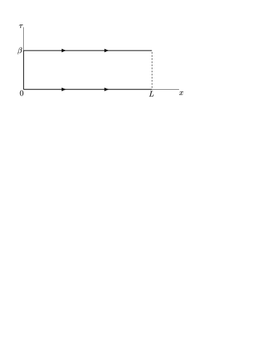
Figure 1: The space-time is periodic in imaginary time $\tau$, with period $\beta$. The boundary is at $x=0$.

The stress-energy tensor $T_{\mu\nu}(x,\tau)$ expresses the response of the system to an infinitesimal local variation of the metric, $g_{\mu\nu}\rightarrow\delta_{\mu\nu}+\delta g_{\mu\nu}(x,\tau)$,

$$\delta\ln Z=(1/2)\int\!\!\!\int\mu^{2}\mathrm{d}\tau\mathrm{d}x\,\langle\delta g_{\mu\nu}T^{\mu\nu}(x,\tau)\rangle\,.$$ (4)

We specialize to 1+1 dimensions the general analysis of the stress-energy tensor in space-times with boundaryMcAvity and Osborn (1993). The stress-energy tensor can be written as a bulk part plus a boundary part

$$\delta\ln Z=(1/2)\int\!\!\!\int\mu^{2}\mathrm{d}\tau\mathrm{d}x\,\langle\delta g_{\mu\nu}T_{\mathit{b}ulk}^{\mu\nu}(x,\tau)\rangle+(1/2)\int_{0}^{\beta}\mu\mathrm{d}\tau\,\langle\delta g_{\mu\nu}(0,\tau)t^{\mu\nu}(\tau)\rangle$$

$$T_{\mu\nu}=T^{\mathit{b}ulk}_{\mu\nu}(x,\tau)+\delta(\mu x)t_{\mu\nu}(\tau)\,.$$ (5)

There could also be a boundary operator proportional to $\delta^{\prime}(x)\mathbf{1}$, but the identity operator makes no contribution to connected correlation functions, so we can ignore it.

The conservation equations follow from invariance of the physics under localized coordinate reparametrizations $\delta x^{\mu}=v^{\mu}(x,\tau)$ where the vector field $v^{\mu}$ is tangent to the boundary, i.e. $v^{x}(0,\tau)=0$. The coordinate reparametrization is equivalent to a change in the metric tensor $\delta g_{\mu\nu}=\partial_{\mu}v_{\nu}+\partial_{\nu}v_{\mu}\,.$ Plugging this into the formula for $\delta\ln Z$ and setting the variation to zero we obtain, after integration by parts, the bulk conservation equation $\partial^{\mu}T^{\mathit{b}ulk}_{\mu\nu}=0$ and also

$$\int\mu\mathrm{d}\tau\,\left(\mu T^{\mathit{b}ulk}_{x\tau}v^{\tau}-t_{\mu\nu}\partial^{\mu}v^{\nu}\right)=0\,.$$

at the boundary, which is equivalent to the boundary conservation equations $t_{xx}=t_{x\tau}=t_{\tau x}=0$ and

$$\mu T^{\mathit{b}ulk}_{x\tau}(0,\tau)+\partial_{\tau}\theta(\tau)=0$$ (6)

where $\theta(\tau)\equiv t_{\tau\tau}(\tau)$. The boundary operator $\theta$ was described in Ref. Ghoshal and Zamolodchikov (1994).

The trace of the stress-tensor is

$$T_{\mu}^{\mu}=\Theta(x,\tau)=\Theta_{\mathit{b}ulk}(x,\tau)+\delta(\mu x)\theta(\tau)\,.$$ (7)

The system is critical in the bulk, so $\Theta_{\mathit{b}ulk}(x,\tau)=0$ up to contact terms. The full trace is $\Theta=\delta(\mu x)\theta(\tau)$, entirely a boundary operator.

The space of boundary conditions is parameterized by the coupling constants $\lambda^{a}$ which couple to the renormalized local boundary fields $\phi_{a}$

$$\partial_{a}\ln Z=\int\mu\mathrm{d}\tau\,\langle\phi_{a}(\tau)\rangle\,.$$

The boundary trace $\theta$ can be decomposed into a linear combination of the boundary fields and the identity operator

$$\theta\ =\beta^{a}(\lambda)\phi_{a}+h(\lambda)\mathbf{1}$$ (8)

where the coefficients $\beta^{a}(\lambda)$ are the boundary $\beta$-functions. We will not have to worry about the term $h(\lambda)\mathbf{1}$, because $\theta$ will only appear within connected correlation functions.

The foregoing are operator statements. In correlation functions, the stress-energy tensor will also have contact terms. The generator of dilatations $\delta g_{\mu\nu}=2(\delta\mu/\mu)\delta_{\mu\nu}$ is $\int\!\!\!\int\mu^{2}\mathrm{d}\tau\mathrm{d}x\,\Theta(x,\tau)$ so the renormalization group equation for $\ln Z$ is

$$(\mu\partial/\partial\mu)\ln Z = \int\!\!\!\int\mu^{2}\mathrm{d}\tau\mathrm{d}x\,\langle\Theta(x,\tau)\rangle$$ (9)

$$= \int\!\!\!\int\mu^{2}\mathrm{d}\tau\mathrm{d}x\,\langle\delta(x)\theta(\tau)+\Theta_{\mathit{b}ulk}(x,\tau)\rangle_{c}$$

$$= \beta^{a}\partial_{a}\ln Z+\mu\beta h(\lambda)\,.$$

For the one-point functions,

$$(\mu\partial/\partial\mu)\langle\phi_{b}(\tau_{1})\rangle = \int\!\!\!\int\mu^{2}\mathrm{d}\tau\mathrm{d}x\,\langle\Theta(x,\tau)\phi_{b}(\tau_{1})\rangle_{c}$$ (10)

$$= \int\!\!\!\int\mu^{2}\mathrm{d}\tau\mathrm{d}x\,\langle\left[\delta(x)\theta(\tau)+\Theta_{\mathit{b}ulk}(x,\tau)\right]\phi_{b}(\tau_{1})\rangle_{c}$$

$$= \beta^{a}\partial_{a}\langle\phi_{b}(\tau_{1})\rangle+(\gamma^{a}_{b}-\delta^{a}_{b})\langle\phi_{a}(\tau_{1})\rangle$$

where the coefficients $\gamma^{a}_{b}-\delta^{a}_{b}$ come from contact terms of $\Theta_{\mathit{b}ulk}$ and $\theta$ with $\phi_{a}$. Because of the contact terms, $\Theta_{\mathit{b}ulk}$ cannot be omitted. The identity $\gamma^{a}_{b}=\partial_{b}\beta^{a}$ follows from $[\mu\partial/\partial\mu,\partial_{a}]=0$, which in turn follows from the definition of the $\lambda^{a}$ as the coupling constants renormalized at scale $\mu$.

We will need one last property of the stress-energy tensor, that $T^{\mathit{b}ulk}_{\mu\nu}(x,\tau)$ decays as $\exp(-4\pi x/\beta)$ in connected correlation functions far from the boundary. When $x$ is far from the boundary, $T^{\mathit{b}ulk}_{\mu\nu}(x,\tau)$ behaves as in the bulk theory without boundary. The exponential decay condition expresses the conformal invariance of the bulk critical system. It is derived using the interpretation of Fig. 1 in which space and imaginary time are exchanged. Space becomes a circle of length $\beta$. The correlation functions become the expectation values $\langle B|\cdots|0\rangle$ where $|0\rangle$ is the ground state of the bulk critical system on the circle, and $\langle B|$ is the state representing the boundary condition. Using the complex coordinate $w=2\pi(x+i\tau)/\beta$, the bulk stress-energy tensor takes the form $T^{\mathit{b}ulk}_{xx}=T^{\mathit{b}ulk}_{\tau\tau}=T(w)+\bar{T}(\bar{w})$, $T^{\mathit{b}ulk}_{x\tau}=i(T(w)-\bar{T}(\bar{w}))$, where $T(w)=\sum_{n}L_{n}\exp(-nw)$ and $\bar{T}(\bar{w})=\sum_{n}\bar{L}_{n}\exp(-n\bar{w})$, $n$ ranging from ${-}\infty$ to ${+}\infty$, the $L_{n}$ and $\bar{L}_{n}$ being the Virasoro operators. Bulk conformal invariance means $L_{1}|0\rangle=\bar{L}_{1}|0\rangle=0$. Therefore, $T(w)\sim\exp(-2w)$ and $T(\bar{w})\sim\exp(-2\bar{w})$ in connected correlation functions, far from the boundary. So $T^{\mathit{b}ulk}_{\mu\nu}(x,\tau)\sim\exp(-4\pi x/\beta)$.

III The proof

We prove the gradient formula, Eq. 3, with the metric on the space of boundary conditions given by

$$g_{ab}(\lambda)=\int\mu\mathrm{d}\tau_{1}\int\mu\mathrm{d}\tau\,\langle\phi_{a}(\tau_{1})\phi_{b}(\tau)\rangle_{c}\left(1-\cos\left[2\pi(\tau-\tau_{1})/\beta\right]\right)\,.$$ (11)

This is essentially the metric proposed in Ref. Witten (1992), except that Ref. Witten (1992) used the un-normalized, full two-point function, while we use the normalized, connected two-point function. Because we are using the connected two-point function, we can write

$$g_{ab}\beta^{b}=\int\mu\mathrm{d}\tau_{1}\int\mu\mathrm{d}\tau\,\langle\phi_{a}(\tau_{1})\theta(\tau)\rangle_{c}\left(1-\cos\left[2\pi(\tau-\tau_{1})/\beta\right]\right)\,.$$ (12)

The identity component of $\theta$ makes no contribution to the connected two-point function. Let us deal with the term containing the cosine:

$$A_{a}(\tau_{1}) \equiv \int\mu\mathrm{d}\tau\langle\phi_{a}(\tau_{1})\theta(\tau)\rangle_{c}\left(-\cos\left[2\pi(\tau-\tau_{1})/\beta\right]\right)$$ (13)

$$= \int\mu\mathrm{d}\tau\langle\phi_{a}(\tau_{1})\partial_{\tau}\theta(\tau)\rangle_{c}(\beta/2\pi)\sin\left[2\pi(\tau-\tau_{1})/\beta\right]$$

We have integrated by parts on the boundary to obtain the second equation. The correlation functions are distributions, so integration by parts is justified. By the boundary conservation law Eq. 6,

$$A_{a}(\tau_{1})=\int\mu\mathrm{d}\tau\,\langle\phi_{a}(\tau_{1})\mu T^{\mathit{b}ulk}_{x\tau}(\tau)\rangle_{c}(-2)v^{\tau}(0,\tau)$$ (14)

where we define $v^{\tau}(0,\tau)\equiv(\beta/4\pi)\sin\left[2\pi(\tau-\tau_{1})/\beta\right]$ as a tangent vector field on the boundary. Next, we extend the boundary vector field $v^{\tau}(0,\tau)$ to a conformal Killing vector field $v^{\mu}(x,\tau)$ in the bulk. That is, $v^{x}(0,\tau)=0$ and $\partial_{\mu}v_{\nu}+\partial_{\nu}v_{\mu}=g_{\mu\nu}\partial_{\sigma}v^{\sigma}$. Such a vector field is most easily found as an analytic vector field $v^{w}=(2\pi/\beta)(v^{x}+iv^{\tau})$ in the complex coordinate $w=2\pi(x+i\tau)/\beta$,

$$v^{w} = (2\pi/\beta)(v^{x}+iv^{\tau})=\left[\exp(w-w_{1})-\exp(-w+w_{1})\right]/4$$

$$\bar{v}^{\bar{w}} = (2\pi/\beta)(v^{x}-iv^{\tau})=\left[\exp(\bar{w}-\bar{w}_{1})-\exp(-\bar{w}+\bar{w}_{1})\right]/4\,.$$

Then

$$\partial_{\sigma}v^{\sigma}=\partial_{w}v^{w}+\partial_{\bar{w}}\bar{v}^{\bar{w}}=\cos\left[2\pi(\tau-\tau_{1})/\beta\right]\cosh(2\pi x/\beta)\,.$$

Now we integrate by parts in the bulk, using the bulk conservation equation, to obtain

$$A_{a}(\tau_{1})=\int\!\!\!\int\mu^{2}\mathrm{d}\tau\mathrm{d}x\,\langle\phi_{a}(\tau_{1})T^{\mathit{b}ulk}_{\mu\nu}(x,\tau)\rangle_{c}(\partial^{\mu}v^{\nu}+\partial^{\nu}v^{\mu})\,.$$ (15)

There is no boundary term at large $x$ because of the decay condition $T^{\mathit{b}ulk}_{\mu\nu}(x,\tau)\sim\exp(-4\pi x/\beta)$. Then we use the fact that $v^{\mu}$ is a conformal Killing vector to write

$$A_{a}(\tau_{1})=\int\!\!\!\int\mu^{2}\mathrm{d}\tau\mathrm{d}x\,\langle\phi_{a}(\tau_{1})\Theta_{\mathit{b}ulk}(x,\tau)\rangle_{c}\partial_{\sigma}v^{\sigma}\,.$$ (16)

Finally, we can approximate $\partial_{\sigma}v^{\sigma}\sim 1$, because $\Theta_{\mathit{b}ulk}=0$ except for contact terms. The error term is

$$\int\!\!\int\mu^{2}\mathrm{d}\tau\mathrm{d}x\,\langle\phi_{a}(\tau_{1})\Theta_{\mathit{b}ulk}(x,\tau)\rangle_{c}(\partial_{\sigma}v^{\sigma}-1)\,.$$

The boundary operator $\phi_{a}(\tau_{1})$ is renormalizable, and $\Theta_{\mathit{b}ulk}$ has dimension $2$, so the most singular contact terms in the two-point function are of the form $\delta(x)\delta^{\prime}(\tau-\tau_{1})$ and $\delta^{\prime}(x)\delta(\tau-\tau_{1})$. But $\partial_{\sigma}v^{\sigma}(x,\tau)-1$ vanishes to second order at $x=0$, $\tau=\tau_{1}$, so there is no error. Thus

$$A_{a}(\tau_{1})=\int\!\!\!\int\mu^{2}\mathrm{d}\tau\mathrm{d}x\,\langle\phi_{a}(\tau_{1})\Theta_{\mathit{b}ulk}(x,\tau)\rangle_{c}\,.$$ (17)

Using Eq. 17 in Eq. 12, we arrive at

$$g_{ab}\beta^{b} = \int\mu\mathrm{d}\tau_{1}\int\!\!\int\mu^{2}\mathrm{d}\tau\mathrm{d}x\,\langle\phi_{a}(\tau_{1})\left[\delta(\mu x)\theta(\tau)+\Theta_{\mathit{b}ulk}(x,\tau)\right]\rangle_{c}$$ (18)

$$= \int\mu\mathrm{d}\tau_{1}\int\!\!\int\mu^{2}\mathrm{d}\tau\mathrm{d}x\,\langle\phi_{a}(\tau_{1})\Theta(x,\tau)\rangle_{c}$$

$$= \int\mu\mathrm{d}\tau_{1}(\mu\partial/\partial\mu)\langle\phi_{a}(\tau_{1})\rangle$$

$$= (\mu\partial/\partial\mu-1)\partial_{a}\ln Z$$

$$= \partial_{a}(\mu\partial/\partial\mu-1)\ln Z$$

$$= -\partial_{a}s$$

which is the gradient formula.

IV Comments on the gradient formula

Each element of the gradient formula is covariant under renormalization. The boundary entropy $s$ is covariant under renormalization, $\mu\partial s/\partial\mu=\beta^{a}\partial_{a}s$, even though the partition function is not (see Eq. 9). Using Eq. 9,

$$(\mu\partial/\partial\mu-\beta^{a}\partial_{a})s = (\mu\partial/\partial\mu-\beta^{a}\partial_{a})(1-\mu\partial/\partial\mu)\ln Z$$ (19)

$$= (1-\mu\partial/\partial\mu)(\mu\partial/\partial\mu-\beta^{a}\partial_{a})\ln Z$$

$$= (1-\mu\partial/\partial\mu)(\mu\beta h)=0\,.$$

That is, the entropy is not sensitive to a shift of the ground state energy. The covariance of $\beta^{a}$ is just its $\mu$-independence. The metric $g_{ab}$ is covariant under renormalization because it is defined in terms of normalized, connected correlation functions, in Eq. 11.

To show that the metric $g_{ab}$ is positively definite, we need only remark that $g_{ab}\delta\lambda^{a}\delta\lambda^{b}$ is given in Eq. 11 as a positive two point function of $\phi=\delta\lambda^{a}\phi_{a}$, integrated against a positive function.

The cosine term in the metric plays a twofold role. On the one hand, it provides the $\Theta_{bulk}$ term in the correlation function of $\Theta$ with the boundary operator. On the other hand the cosine term renders the metric independent of contact terms in the two-point functions of the boundary operators. Such terms could spoil the positivity of the metric. The metric, as defined by Eq. 11, is independent of contact terms. During the proof of the gradient formula, we split it into two parts, each of which does depend on the contact terms. At that point, the two point functions have to be treated as distributions. In the end, when the two terms are joined together, the result is independent of the contact terms. The technical roles of the cosine term are evident, but we do not see a deeper meaning. The cosine first appeared in the string theory metric proposed in Ref. Witten (1992). But the proposal was not natural in string theory, as it involved integrating dimension zero fields. So we still do not see a natural interpretation of the cosine term.

V Relation with string theory

The conjectured string theory gradient formula involves an additional boundary coupling constant $\lambda^{0}$ which couples to the identity operator $\phi_{0}=\mathbf{1}$. The string partition function is

$$Z_{\mathit{s}}=\exp(\mu\beta\lambda^{0})z(\mu\beta)$$

where $z(\mu\beta)$ is the boundary partition function, from Eq. 1. The string $\beta$-function, $\beta_{\mathit{s}}^{a}$, is the ordinary $\beta^{a}$ for the ordinary coupling constants, plus, from Eq. 9, $\beta_{\mathit{s}}^{0}=\lambda^{0}+h(\lambda)$. The conjectured string theory gradient formula is

$$G^{\mathit{s}}_{ab}\beta_{\mathit{s}}^{b}=-\partial_{a}g_{\mathit{s}}$$

where

$$g_{\mathit{s}}=(1-\mu\partial/\partial\mu)Z_{\mathit{s}}$$

and the string metric is

$$G^{\mathit{s}}_{ab}(\lambda)=\int\mu\mathrm{d}\tau_{1}\int\mu\mathrm{d}\tau\,Z_{\mathit{s}}\langle\phi_{a}(\tau_{1})\phi_{b}(\tau)\rangle\left(1-\cos\left[2\pi(\tau-\tau_{1})/\beta\right]\right)\,.$$ (20)

These string formulas are un-physical, when applied to 1-d quantum systems. No physical probe couples to the identity operator $\phi_{0}=\mathbf{1}$, so $\lambda^{0}$ is not a physical coupling constant. Un-normalized correlation functions are not measurable. Changes in $g_{\mathit{s}}$ are not locally measurable, because $g_{\mathit{s}}$ is constructed from $z$, not $\ln z$. On the other hand, all of the elements of the physical gradient formula, Eq. 3, can by measured by local operations at the boundary of the 1-d system. The string gradient formula is formally sensible from the string theory perspective. The $\lambda^{a}$ are the wave-modes of spacetime fields, $\lambda^{0}$ is the zero-mode of the tachyon field. The equation $\beta_{\mathit{s}}^{a}=0$ has the form of a space-time equation of motion. The function $g_{\mathit{s}}(\lambda)$ has the form of a space-time action.

The un-physical parameter $\lambda^{0}$ can be eliminated by extremizing $g_{\mathit{s}}$Kutasov et al. (2000); Moore . We carry out this idea. We calculate that $\partial g_{\mathit{s}}/\partial\lambda^{0}=0$ at $\lambda^{0}=a_{0}$, $\mu\beta a_{0}=-\mu\partial\ln z/\partial\mu$. We calculate that, at $\lambda^{0}=a_{0}$, $g_{\mathit{s}}=Z_{\mathit{s}}=z\exp(\mu\beta a_{0})$, which is the physical quantity $\exp(s)$. It now becomes straightforward to show the equivalence between the string gradient formula and the physical gradient formula. The string gradient formula is trivial in the direction of $\lambda^{0}$, and is precisely the physical formula on the subspace $\lambda^{0}=a_{0}$. To be explicit, the components of the string metric are $G^{\mathit{s}}_{00}=(\mu\beta)^{2}Z_{\mathit{s}}$, $G^{\mathit{s}}_{0b}=\mu\beta Z_{\mathit{s}}\partial_{a}\ln Z_{\mathit{s}}$, $G^{\mathit{s}}_{ab}=Z_{\mathit{s}}(g_{ab}+\partial_{a}\ln Z_{\mathit{s}}\partial_{b}\ln Z_{\mathit{s}})$, where the indices $a,b$ now range only over the physical coupling constants. The string gradient formula splits into two equations

$$G^{\mathit{s}}_{00}\beta_{\mathit{s}}^{0}+G^{\mathit{s}}_{0b}\beta^{b}=-\partial_{0}g_{\mathit{s}}$$

$$G^{\mathit{s}}_{a0}\beta_{\mathit{s}}^{0}+G^{\mathit{s}}_{ab}\beta^{b}=-\partial_{a}g_{\mathit{s}}\,.$$

The first is satisfied identically, it is just the rg equation for $Z_{\mathit{s}}$,

$$\mu\partial Z_{\mathit{s}}/\partial\mu=(\beta^{a}\partial_{a}+\mu\beta\beta_{\mathit{s}}^{0})Z_{\mathit{s}}\,.$$

The second equation, after substituting and then using the rg equation for $Z_{\mathit{s}}$, becomes

$$Z_{\mathit{s}}g_{ab}\beta^{b}=Z_{\mathit{s}}(-1+\mu\partial/\partial\mu)\partial_{a}\ln Z_{\mathit{s}}$$

which is exactly the physical gradient formula, since $\partial_{a}\ln Z_{\mathit{s}}=\partial_{a}\ln Z$. So, by proving the physical gradient formula, we have also proved the string gradient formula.

We would like to thank Gregory Moore and Alexander Zamolodchikov for stimulating discussions. We especially thank Gregory Moore for pointing out a deficiency in an early version of the proof. This work was supported by the Rutgers New High Energy Theory Center, which A. K. thanks for warm hospitality. The work of A. K. was supported in part by BSF-American-Israel Bi-National Science Foundation, the Israel Academy of Sciences and Humanities-Centers of Excellence Program, the German-Israel Bi-National Science Foundation.

References

• Affleck and Ludwig (1991) I.Β Affleck and A.Β W. Ludwig, Phys.Β Rev.Β Lett. 67, 161 (1991).
• Affleck and Ludwig (1993) I.Β Affleck and A.Β W. Ludwig, Phys.Β Rev. B48, 7297 (1993).
• Witten (1992) E.Β Witten, Phys.Β Rev. D46, 5467 (1992), eprint hep-th/9208027.
• Witten (1993) E.Β Witten, Phys.Β Rev. D47, 3405 (1993), eprint hep-th/9210065.
• Shatashvili (1993a) S.Β Shatashvili, Phys.Β Lett. B311, 83 (1993a), eprint hep-th/9303143.
• Shatashvili (1993b) S.Β Shatashvili, Alg.Β Anal. 6, 215 (1993b), eprint hep-th/9311177.
• Kutasov etΒ al. (2000) D.Β Kutasov, M.Β Marino, and G.Β Moore, JHEP 10, 45 (2000), eprint hep-th/0009148.
• Konechny (2004) A.Β Konechny, IJMP A19, 2545 (2004), eprint hep-th/0310258.
• (9) G.Β Moore, private communication.
• Friedan (1999, 2003) D.Β Friedan (1999, 2003), two notes on conformal boundary conditions for the $c=1$ gaussian model, unpublished, http://www.physics.rutgers.edu/pages/friedan/.
• Tseng (2002) S.-L. Tseng, JHEP 04, 51 (2002), eprint hep-th/0201254.
• Elitzur etΒ al. (1999) S.Β Elitzur, E.Β Rabinovici, and G.Β Sarkissian, Nucl. Phys. B541, 246 (1999), eprint hep-th/9807161.
• McAvity and Osborn (1993) D.Β M. McAvity and H.Β Osborn, Nucl. Phys. B406, 655 (1993), eprint hep-th/9302068.
• Ghoshal and Zamolodchikov (1994) S.Β Ghoshal and A.Β Zamolodchikov, Int.Β J.Β Mod.Β Phys. A9, 3841 (1994), erratum ibid. A9 (1994) 4353, eprint hep-th/9306002.