Exact solutions for Bianchi type cosmological metrics, Weyl orbits of $E_{8(8)}$ subalgebras and $p$–branes ^†
P. Fré¹, K. Rulik¹, M. Trigiante²

¹ Dipartimento di Fisica Teorica, Universitá di Torino, $\&$ INFN - Sezione di Torino

via P. Giuria 1, I-10125 Torino, Italy

² Dipartimento di Fisica Politecnico di Torino, C.so Duca degli Abruzzi, 24, I-10129 Torino

In this paper we pursue further a programme initiated in a previous work and aimed at the construction, classification and property investigation of time dependent solutions of supergravity (superstring backgrounds) through a systematic exploitation of $\mathrm{U}$–duality hidden symmetries. This is done by first reducing to $D=3$ where the bosonic part of the theory becomes a sigma model on $E_{8(8)}/SO(16)$, solving the equations through an algorithm that produces general integrals for any chosen regular subalgebra $\mathbf{G}_{r}\subset E_{8(8)}$ and then oxiding back to $D=10$. Different oxidations and hence different physical interpretations of the same solutions are associated with different embeddings of $\mathbf{G}_{r}$. We show how such embeddings constitute orbits under the Weyl group and we study the orbit space. This is relevant to associate candidate superstring cosmological backgrounds to space $Dp$–brane configurations that admit microscopic descriptions. In particular in this paper we show that there is just one Weyl orbit of $A_{r}$ subalgebras for $r<6$. The orbit of the previously found $A_{2}$ solutions, together with space–brane representatives contains a pure metric representative that corresponds to homogeneous Bianchi type 2A cosmologies in $D=4$ based on the Heisenberg algebra. As a byproduct of our methods we obtain new exact solutions for such cosmologies with and without matter. We present a thorough investigation of their properties.

 ^† This work is supported in part by the European Union RTN contracts HPRN-CT-2000-00122 and HPRN-CT-2000-00131.

1 Introduction

Cosmological solutions of supergravity or, more generally, time dependent superstring backgrounds have attracted a great deal of interest in the recent years [1, 2, 3, 4, 5, 6, 7, 8, 9, 10, 11, 12, 13, 14, 15, 16], both because of the stimulus provided by new data in observational cosmology [17], which seem to imply a small but non vanishing cosmological constant a flat geometry of the universe and confirm inflation [18], and also for intrinsic conceptual reasons inherent to a continuously sought for deeper understanding of the internal structure of the theory.

Relying on the motivations outlined above, in a recent paper [19] we have addressed the question of establishing a general classification of all time dependent backgrounds of ten dimensional superstring, providing also an algorithm capable of constructing explicit analytic solutions of supergravity field equations. Our method is based on a systematic use of $\mathrm{U}$–duality and exploits the algebraic structure of hidden symmetries. Indeed we heavily relied on the observation that looking for solutions that depend only on one–parameter is tantamount as dimensionally reducing the theory to $1+0$ dimensions. It is also equivalent to looking at one–parameter (time) solutions of the theory reduced to any dimension $d$ in the interval

$$1+0\leq d\leq 1+9$$ (1.1)

Preferred choice for us was $d=1+2$ since, there, all bosonic degrees of freedom correspond to scalar fields and supergravity is replaced by the sigma model $\mathrm{E_{8(8)}}/\mathrm{SO(16)}$. Using the solvable Lie algebra representation of non–compact cosets we were able to rewrite the sigma model field equations in Nomizu operator form and construct an algorithm that allows:

a

to obtain analytic exact solutions of the $D=3$ equations in a systematic way,

b

to oxide back such solutions to $D=10$ supergravity backgrounds by following precise algebraic oxidation rules based on a one-to-one correspondence between the $D=10$ fields and the $8$ Cartan generators plus $120$ positive roots of $E_{8(8)}$.

In particular in [19] we proved that the possible $D=3$ solutions are classified by regularly embedded subalgebras $\mathbf{G}_{r}\subset\mathrm{E_{8}}$ of rank $r\leq 8$ and that their ten–dimensional physical interpretation (oxidation) depends on the classification of the different embeddings $\mathbf{G}_{r}\hookrightarrow\mathrm{E_{8}}$. We gave some preliminary examples of explicit solutions based on the simplest choice $\mathbf{G}_{r}=\mathrm{A_{2}}$. It also turned out that these solutions provide a smooth and exact realization of the bouncing phenomenon on Weyl chamber walls envisaged by the cosmological billiards of Damour et al. [20, 21, 22, 23, 24, 25, 26, 27, 28, 29, 30]. We also showed how this physical phenomenon was triggered by the presence of extended objects possibly interpretable, at the microscopic level, as space $Dp$–branes.

In the present paper we address and answer the important related question: How many different orbits of cosmological solutions are there under the full $U$–duality group? It is interesting per se to know that apparently completely different classical configurations are related by duality transformations but an exhaustive organization of $\mathrm{U}$–orbits has a specific intrinsic value in view of the following consideration that was already systematically exploited in the case of supersymmetric black–holes [31]. Suppose that a certain configuration of supergravity fields is in the same $\mathrm{U}$–orbit as another one which can be solely described in terms of Ramond–Ramond $p$–forms and therefore of $D$–branes. It follows that a microscopic stringy description is available for all configurations sitting in that orbit. Any stringy calculation which might be of interest can be performed for the orbit representative where the $D$–brane description is available and the results can be exported, via $\mathrm{U}$–duality, to all the other cases for which a $D$–brane boundary state cannot be constructed. This way of reasoning was for instance used in [31] to calculate the statistical entropy of black–holes and verify that it coincides with the area of the event horizon. After constructing a generating solution of $\mathcal{N}=8$ black–holes, that depends on $5$–parameters, and deriving its orbit under the $\mathrm{U}$–duality group $\mathrm{E_{7(7)}}$ it was possible to identify the $Dp$–brane systems that corresponds to specific representatives of the orbit. There one could perform the microscopic calculation of the statistical entropy.

A similar situation can now be realized in the context of cosmological, rather than black–hole solutions. By a systematic study of $\mathrm{U}$–orbits we can connect time–dependent backgrounds of Neveu-Schwarz character, for instance purely gravitational solutions, which might have special physical interest but do not admit $D$–brane descriptions to others that are realized by $D$–brane systems, in particular by space–branes.

A noticeable example of such relations, which has by itself a special interest, will be illustrated in the present paper.

Approximately ninety years ago, just after General Relativity was introduced, Bianchi classified $D=4$ cosmological metrics that are homogeneous [32], namely that admit a three parameter group of isometries acting transitively on constant time slices. Bianchi metrics are of the following form

$$ds^{2} = -A(t)\,dt^{2}+h_{ij}(t)\,\Omega^{i}\,\otimes\,\Omega^{j}$$ (1.2)

where

$$h_{ij}(t)\mbox{ is a symmetric, time dependent $3\times 3$-matrix }$$ (1.3)

and where $\Omega^{i}$ are the Maurer Cartan $1$–forms on a three–dimensional group manifold:

$$d\Omega^{i} = t^{i}_{\phantom{i}{jk}}\Omega^{j}\,\wedge\,\Omega^{k}\quad;\quad\left(\mbox{Maurer Cartan eq.s}\right)$$

$$t^{i}_{\phantom{i}{jk}} =$$ structure constants of a three parameter Lie algebra (1.4)

Bianchi classification of homogeneous cosmologies is a classification of all three–dimensional algebras $\mathcal{G}_{3}$, identified by the structure constants $t^{i}_{\phantom{i}{jk}}$, a classification that includes all non–semisimple and solvable algebras. Once the algebra $\mathcal{G}_{3}$ is chosen, one is still confronted with the task of solving Einstein equations for the generalized scale factors $A(t)$ and $h_{ij}(t)$ in presence of suitable matter encoded into a suitable stress–energy tensor. Here the list of exact analytic solutions is not abundant [32] since the differential equations to be solved have for most algebras, except the abelian $\mathbb{R}^{3}$, a rather formidable non linear structure that impedes to obtain general or particular integrals.

As a by–product of our orbit analysis we will present some exact analytic solutions of Einstein equations for homogeneous cosmologies that, up to our knowledge, were so far unknown in the literature.

Specifically we will prove the following. Among the various three parameter algebras one has the Heisenberg algebra defined by the following Maurer–Cartan equations:

$$d\Omega^{1}+\frac{\varpi}{2}\,\Omega^{2}\wedge\Omega^{3}=0$$

$$d\Omega^{2}=0$$ (1.5)

$$d\Omega^{3}=0$$ (1.6)

or, alternatively, by the commutation relations of the dual generators $\Omega^{i}(T_{j})=\delta^{i}_{j}$:

$$Heis :$$

$$\left[T_{i},T_{j}\right] = t_{ij}^{k}\,T_{k}\quad;\quad t_{23}^{1}=-\frac{\varpi}{4}\quad\quad;\quad\mbox{all other components of $t_{ij}^{k}$ vanish}$$ (1.7)

In the standard nomenclature, homogeneous cosmologies based on the algebra (1.6) are named spaces of Bianchi type 2A. We shall prove that all possible oxidations of the $\mathrm{A_{2}}$ sigma model solutions found in [19] are in the same $\mathrm{U}$–orbit together with a purely gravitational representative corresponding to a $D=4$ Bianchi type 2A space times a $\mathrm{T^{6}}$ torus or a reduction thereof. More specifically we have Bianchi type 2A spaces that are exact solutions for either the dilaton gravity lagrangian in $d=4$

$$A_{\mbox{dilaton gravity}}=\int\,\sqrt{-\mbox{det}\,g}\,\left\{2\,R[g]\,-{\textstyle\frac{1}{2}}\,\partial^{\mu}\phi\,\partial_{\mu}\phi\right\}$$ (1.8)

or for the $0$–brane $d=4$ lagrangian

$$A_{\mbox{0-brane}}=\int\,\sqrt{-\mbox{det}\,g}\,\left\{2\,R[g]\,-{\textstyle\frac{1}{2}}\,\partial^{\mu}\phi\,\partial_{\mu}\phi+{\textstyle\frac{1}{4}}\,\exp[-a\,\phi]\,F_{\mu\nu}\,F^{\mu\nu}\right\}$$ (1.9)

This follows from what we are going to show shortly, namely that, up to conjugation, there is just one regular embedding

$${\bf i}:\mathrm{A_{2}}\,\,\hookrightarrow\,\mathrm{E_{8}}$$ (1.10)

This result has two relevant implications. The first, which we extensively discuss in the present paper, is that, through this argument, we retrieve new exact solutions of Bianchi type 2A. The second implication is that, via $\mathrm{U}$–transformations, such new solutions, whose potential interest in cosmology is evident, are dual to solutions made of $D$-branes and admitting a microscopic description in terms of time–dependent boundary states. Indeed in [19] we already oxided the $\mathrm{A_{2}}$ sigma model solution to a $D=10$ configuration containing a diagonal metric plus a system composed of a $D3$ space–brane and a $D1$ space–string. Due to the uniqueness of the orbit, Bianchi cosmology 2A and this system are dual.

Our method to study $\mathrm{U}$–orbits is based on the following preliminary steps. Thanks to the techniques developed in [19] we know that each solution is obtained in the following way. Let $\mathbf{G}_{r}\subset E_{8(8)}$ be a regularly embedded maximally non compact subalgebra of the $\mathrm{U}$–duality algebra of rank $r$. Let $\mathbf{H}_{r}\subset\mathbf{G}_{r}$ be its maximal compact subalgebra which is also necessarily contained in the maximal compact subalgebra of $E_{8(8)}$ namely $\mathbf{H}_{r}\,\subset\,\mathrm{SO(16)}$. Let furthermore $\mathcal{H}_{r}\subset\mathbf{G}_{r}$ be the Cartan subalgebra of the chosen $\mathbf{G}_{r}$ which is necessarily a subalgebra $\mathcal{H}_{r}\subset\mathcal{H}_{8}$ of the $E_{8(8)}$ Cartan subalgebra. The $\mathbf{G}_{r}$-solution is obtained from a generating solution that lies only in the Cartan subalgebra $\mathcal{H}_{r}$ by means of a compensating $\mathbf{H}_{r}$ transformation. The $\mathrm{U}$–orbit of the $\mathbf{G}_{r}$-solution is given by the orbit of possible regular embeddings:

$${\bf i}\,:\,\mathbf{G}_{r}\hookrightarrow\mathrm{E_{8}}$$ (1.11)

To this effect it is necessary and sufficient to restrict one’s attention to the discrete Weyl group $\mathcal{W}\subset\mathrm{U}$. Indeed $\mathcal{W}$ maps the Cartan subalgebra into itself and permutes the set of roots. $\mathrm{U}$–duality orbits of $\mathbf{G}_{r}$ solutions are just the Weyl orbits of the $\mathbf{G}_{r}$ root system.

Therefore in this paper we perform a systematic study of the Weyl orbits of $E_{8}$ regular subalgebras. We develop an algorithm for such a study and we explore the nested chain of $\mathrm{A_{r}}$ subalgebras of increasing rank. This chain is particularly important since its canonical realization is within the $\mathrm{A_{6}}\subset\mathrm{E_{8}}$ subalgebra that describes the metric moduli of the $T^{7}$ torus in the reduction from $D=10$ to $D=3$ dimensions. Hence any $\mathrm{A_{r}}$ solution, if the Weyl orbit is unique, has a purely gravitational realization which is dual to other realizations eventually made out of branes. Indeed, from our analysis it appears that there is just one Weyl orbit for $\mathrm{A_{2}}$, $\mathrm{A_{3}}$ up to $\mathrm{A_{6}}$ subalgebras. Beyond we have two orbits corresponding to the type IIA and type IIB interpretations of the theory.

In particular the uniqueness of the $\mathrm{A_{2}}$ orbit is the proof of what we claimed above. Bianchi type 2A cosmologies are dual to suitable space–brane systems.

Our paper is organized as follows:

In section 2 we study the algebraic setup to classify Weyl orbits of regular subalgebras, we outline the physical implications of this classification and we derive our general algebraic results.

In section 3 we study the canonical purely metric representative of the $\mathrm{A_{2}}$ Weyl orbit and we show that it is related to exact solutions of homogeneous Bianchi cosmologies based on the Heisenberg algebra.

In section 4 we perform a detailed study of the new exact solutions of Bianchi type 2A that we have obtained through our construction.

Section 5 contains our conclusions and perspectives.

2 Weyl orbits of $E_{8(8)}$ subalgebras and Oxidation

As we anticipated in the introduction, the problem of classifying different oxidations of the same $\sigma$–model solutions is reduced first to the classifications of embeddings (1.11) and then to the classification of Weyl orbits of the $\mathbf{G}_{r}$ root system within the $E_{8(8)}$ root system.

Let us now review the physical arguments leading to this conclusion.

Using the solvable Lie algebra representation of the $\mathrm{E_{8(8)}/SO(16)}$ coset manifold [34], every one–parameter (time) dependent solution of the $\sigma$–model is described by the map:

$$\mathbb{R}\ni t\,\mapsto\,\left\{h^{i}(t)\,,\,\phi^{\alpha}(t)\right\}\,\equiv\,\Phi(t)\,\in\,Solv\left(E_{8}\right)$$ (2.1)

where $h^{i}(t)$ are the fields associated with the CSA generators, $\phi^{\alpha}(t)$ the fields associated with the positive roots $\alpha>0$ and altogether $\Phi(t)$ is a map of the time–line into the Borel subalgebra $Solv\left(E_{8}\right)\subset E_{8(8)}$.

Oxidation is a uniquely identified procedure that maps $\Phi(t)$ into a solution of either type IIA or type IIB supergravity:

$$Ox\,:\,\Phi(t)\,\mapsto\,F(t)=\mbox{supergravity solution}$$ (2.2)

According to the results of [19] a systematic search of the possible time dependent backgrounds is performed in the following way. First single out a maximally non compact regularly embedded subalgebra ${\bf i}\left[\mathbf{G}_{r}\right]\subset E_{8(8)}$ and let ${\bf i}\left[\mathbf{H}_{r}\right]\subset{\bf i}\left[\mathbf{G}_{r}\right]$ be its compact subalgebra. Here ${\bf i}$ denotes the specific embedding, while $\mathbf{G}_{r}$ denotes the abstract algebra. The pair $\left\{\mathrm{G}_{r}\,,\,\mathrm{H}_{r}\right\}$ defines a new $\sigma$–model with target space $\mathrm{G}_{r}/\mathrm{H}_{r}$ which also admits a solvable Lie algebra description. Hence every one–parameter (time) dependent solution of this new (smaller) $\sigma$–model is described by a map similar to that in (2.1):

$$\mathbb{R}\ni t\,\mapsto\,\left\{h_{G_{r}}^{i}(t)\,,\,\phi_{G_{r}}^{\alpha}(t)\right\}\,\equiv\,\Phi_{G_{r}}(t)\,\in\,Solv\left(\mathbf{G}_{r}\right)$$ (2.3)

Each different embedding (1.11) defines a different explicit solution of the $\mathrm{E_{8(8)}/SO(16)}$ sigma model:

$${\bf i}\left[\Phi_{G_{r}}(t)\right]\,=\,\Phi_{{\bf i}}(t)$$ (2.4)

which through oxidation (2.2) leads to a different supergravity background.

Let us now recall the algorithm developed in [19] in order to obtain general integrals of the $\mathrm{G}_{r}/\mathrm{H}_{r}$ sigma–model differential equations. There we showed that these equations have the structure of geodesic equations for the scalar manifold $\mathrm{G}_{r}/\mathrm{H}_{r}$ and that one can first obtain a generating solution, corresponding to a normal form orientation of the geodesic tangent vector in the origin ($t=0$). Such a normal form orientation is provided by a tangent vector pointing only in the direction of the Cartan generators and can be reached by means of $\mathrm{H}_{r}$ transformations. Indeed the isotropy group has a linear action on the tangent space to the target manifold. The corresponding generating solution has the form:

$$\Phi^{(0)}_{G_{r}}(t)=\left\{\overline{h}_{G_{r}}^{i}(t)\,,\,0\right\}\quad;\quad\overline{h}_{G_{r}}^{i}(t)=\exp[\omega^{i}\,t+c^{i}]$$ (2.5)

A full solution where also the root fields are excited is obtained from the generating solution by means of compensating $\mathrm{H}_{r}$–transformations, namely $\mathrm{H}_{r}$ transformation with parameters $\theta_{G_{r}}(t)$ such that a solvable parametrization of the coset $\mathrm{G}_{r}/\mathrm{H}_{r}$ is mapped into another solvable parametrization. Such a condition is guaranteed by a system of differential equations which is equivalent to the original system to be solved but has the advantage of being already in triangular form and hence reduced to quadratures. Schematically we have:

$$\Phi_{G_{r}}(t)=H\left(\theta_{G_{r}}^{\alpha}(t)\right)\cdot\Phi^{(0)}_{G_{r}}(t)\quad\Rightarrow\quad{\bf i}\left[\Phi_{G_{r}}(t)\right]={\bf i}\left[H\left(\theta_{G_{r}}(t)\right)\right]\cdot{\bf i}\left[\Phi^{(0)}_{G_{r}}(t)\right]$$ (2.6)

where $H\left(\theta_{G_{r}}(t)\right)$ is the compensating transformation. In (2.6) the first is the relation in the abstract algebra $\mathbf{G}_{r}$, while the second is its realization in the specific subalgebra ${\bf i}\left[\mathbf{G}_{r}\right]\subset\mathrm{E_{8}}$. Using these notations we can address the structure of a generic $E_{8(8)}$ transformation that maps one supergravity solution $F_{1}^{G_{r}}(t)$ associated with one embedding ${\bf i}_{1}$ of the Lie algebra $\mathbf{G}_{r}$ to another supergravity solution $F_{2}^{G_{r}}(t)$ associated with a second embedding ${\bf i}_{2}$. It suffices to note that for any two regular embeddings of the same algebra we have:

$${\bf i}_{1}\,\left[\mathbf{G}_{r}\right]\,=\,\mathbf{w}_{12}\,{\bf i}_{2}\,\left[\mathbf{G}_{r}\right]\quad\mbox{where}\quad\mathbf{w}_{12}\,\in\,\mathcal{W}\left(\mathrm{E_{8}}\right)$$ (2.7)

having denoted by $\mathcal{W}\left(\mathrm{E_{8(8)}}\right)$ the Weyl group of the $E_{8(8)}$ algebra. In eq. (2.7) the action of the Weyl group element $\mathbf{w}_{12}$ is the natural one on the algebra. Then we get

$$\Phi_{{\bf i}_{1}[\mathbf{G}_{r}]}(t)=\,\mathbf{w}_{12}\,\Phi_{{\bf i}_{2}[\mathbf{G}_{r}]}(t)$$ (2.8)

Fig.(1) summarizes our understanding of this Weyl mapping between different supergravity backgrounds.

Figure 1: The Weyl group $\mathcal{W}(E_{8})$ maps different embeddings of the same subalgebra $G_{r}$ into $E_{8(8)}$. There is just one abstract solution of the $\mathrm{G}_{r}/\mathrm{H}_{r}$ sigma model that leads to many different physical oxidations related one to the other by Weyl transformations.

From this argument it follows that it is of primary relevance to study orbits of $E_{8(8)}$ subalgebras under the Weyl group. Since each embedding corresponds to a different oxidation, namely to a different $D=10$ interpretation of the same abstract solution, it follows that all oxidations in the same orbit are equivalent under duality transformations.

2.1 Preliminaries on the Weyl group

Every regular embedding of a smaller semisimple subalgebra $\mathbf{G}_{r}$ into a bigger one ($\mathrm{E_{8}}$ in our case) is uniquely specified by the embedding of the small CSA $\mathcal{H}_{r}\subset\mathbf{G}_{r}$ into the big one $\mathcal{H}_{r}\hookrightarrow\mathcal{H}_{8}$. The embedding of the roots follows uniquely, once the embedding of the CSA is given. Vice versa, the choice of the simple roots of the subalgebra $\mathbf{G}_{r}$ inside the root system of the big algebra $E_{8(8)}$ fixes the embedding of the CSA, the relevant map being

$$\alpha\rightarrow h_{\alpha}$$ (2.9)

So, any embedding is specified by a set of Cartan generators associated with the simple roots of the algebra $\mathbf{G}_{r}$ to be embedded:

$${h_{\alpha_{s}}}=h_{i}\cdot\alpha_{s}^{i},\quad s=1,\dots,r$$ (2.10)

where ${h_{i}},\,i=1,\dots 8$ denote any suitable basis of the Cartan subalgebra of $\mathrm{E_{8(8)}}$. To convert one embedding into another, we just have the Weyl group, which, by definition, is generated by the reflections $\sigma_{\gamma}$ with respect to the plane orthogonal to any of the roots $\gamma\in\Delta$:

$$\sigma_{\gamma}\,{\alpha}=\alpha-\langle\alpha\,,\,\gamma\rangle\,\gamma\quad;\quad\langle\alpha\,,\,\gamma\rangle\,\equiv\,2\frac{\alpha\cdot\gamma}{\alpha\cdot\alpha}$$ (2.11)

2.2 Strategy to classify orbits

In this way we have concluded that the main algebraic question to be answered is how to connect by means of Weyl transformations different choices of the simple roots (or of the CSA subalgebra) of a given abstract $\mathbf{G}_{r}$ inside the root system of $E_{8}$. To illustrate our strategy for the solution of such a problem we begin by presenting the Dynkin diagram of $\mathrm{E_{8}}$, which is done in fig.2.

Figure 2: The Dynkin diagrams of $E_{8(8)}$ and the labeling of simple roots

This fixes our conventions and notations for simple roots, which are those of [19]. In that paper we also presented a table listing all the $120$ positive roots, arranged by height and ordered according to our conventions. We will frequently refer to such table for the absolute identification of the roots $\alpha[i]$ by means of a number $i$ ranging from $1$ to $120$. The correspondence between such a number and the Dynkin labels, according to the naming of fig.2, is given in the aforementioned table of [19].

The strategy we adopt in classifying regular embeddings of $\mathbf{G}_{r}$ in terms of Weyl orbits can be summarized as follows. We consider a set of linearly independent roots ${\gamma_{1},\dots,\gamma_{r}}$ of $\mathbf{G}_{r}$, and embed them sequentially within the root system of $\mathrm{{E}_{8(8)}}$ by requiring that the transformations which we use to fix $\gamma_{i+1}$ should belong to the stability subgroup $I^{\gamma_{i}}_{S}\subset\mathcal{W}({\rm E}_{8})$ which, inside the Weyl group, leaves the previously fixed roots $\gamma_{1},\dots,\gamma_{i}$ invariant. Let us list mathematical properties of the Weyl group which we find convenient to recall at this junction. They are proved in many standard textbooks (see for instance [36]):

• all roots of the $\mathrm{E_{8}}$ Lie algebra lie just in one orbit under the action of the Weyl group $\mathcal{W}(\mathrm{E_{8}})$. And, in particular, with the help of the Weyl group $\mathcal{W}(\mathrm{E_{8}})$ we can map any root into the highest root $\alpha[120]$.

• the stability subgroup of any root of $\mathrm{E_{8}}$ under action of the Weyl group $\mathcal{W}(\mathrm{E_{8}})$ is isomorphic to Weyl group $\mathcal{W}(\mathrm{E_{7}})$. Indeed the roots orthogonal to the highest root $\alpha[120]$ are just those whose component $n_{8}$ vanishes and these are the roots of $\mathrm{E_{7}}$,

• weights of fundamental representation of $\mathrm{E}_{r}$ constitute just one orbit under the action of $\mathcal{W}(\mathrm{E}_{r})$ for $r=4,5,6,7$.

Keeping the above facts ready for use we can develop the embedding procedure we sketched above. According to it we encounter a branching in the Weyl–orbits for the $\mathbf{G}_{r}$ Lie algebra embeddings when we there is more than one possible orbit of $I^{\gamma_{i}}_{S}$ in which to choose the root $\gamma_{i+1}$.

2.2.1 Orbits of $\mathrm{A}_{r}$ algebras

We illustrate our method by considering the embeddings of the $\mathbf{G}_{r}=\mathrm{A_{r}}$ algebras, $r=1,\dots,8$. Here we choose as representative roots $\gamma_{i}$ the set of $r$ linearly independent roots arranged in order of decreasing height starting from $\gamma_{1}$ equal to the highest root of $\mathrm{A_{r}}$ and all the other chosen in such a way that we always have:

$$\forall i\neq j\quad:\quad\gamma_{i}\cdot\gamma_{j}=1$$ (2.12)

In intrinsic Dynkin labels of the $\mathrm{A_{r}}$ Lie algebra, the roots satisfying the constraint (2.12) are the following ones:

$$\begin{array}[]{cccccccc}\gamma_{1}&=&(1,1,1,\dots,1)&;&\gamma_{2}&=&(1,1,\dots,1,0)&\dots\\ \gamma_{r-1}&=&(1,1,0,\dots,0,0)&;&\gamma_{r}&=&(1,0,\dots,0,0)&.\end{array}$$ (2.15)

• Choosing $\gamma_{1}$: since ${\rm Adj}({\rm E}_{8(8)})$ contains a single $\mathcal{W}({\rm E}_{8})$–orbit, all choices of $\gamma_{1}$ are connected by Weyl transformations. Moreover the stability group of any ${\rm E}_{8(8)}$ root is $I^{\gamma_{1}}_{S}=\mathcal{W}({\rm E}_{7})$. With respect to ${\rm E}_{7(7)}\times{\rm O}(1,1)$ the adjoint of ${\rm E}_{8(8)}$ branches as follows:

  $${\bf 248} \rightarrow {\bf 133}_{0}+{\bf 56}_{+1}+{\bf 56}_{-1}+{\bf 1}_{+2}+{\bf 1}_{-2}+{\bf 1}_{0}$$ (2.16)

  The root $\gamma_{1}$ coincides with ${\bf 1}_{+2}$ with respect to its own stability group.

• Choosing $\gamma_{2}$: the only possible orbit of $I^{\gamma_{1}}_{S}=\mathcal{W}({\rm E}_{7})$, where a root, defined by a scalar product $\gamma_{1}\cdot\gamma_{i}=1$, can lie is the representation ${\bf 56}_{+1}$. Since all the remaining roots $\{\gamma_{i}\},\quad i=2,\dots,r$, of our set have such a property, all the others also belong to ${\bf 56}_{+1}$. All members of this orbit are connected by Weyl transformations of $\mathcal{W}({\rm E}_{7})$. The stability group of any root (weight) of the ${\bf 56}_{+1}$ is $I^{\gamma_{2}}_{S}=\mathcal{W}({\rm E}_{6})$ (this is the stability group for a pair of roots of ${\rm E}_{8(8)}$, which have scalar product equal to one). With respect to ${\rm E}_{6(6)}\times{\rm O}(1,1)$ the adjoint of ${\rm E}_{7(7)}$ and the representation ${\bf 56}_{+1}$ decompose, respectively:

  $${\bf 133} \rightarrow {\bf 78}_{0}+{\bf 1}_{0}+{\bf 27}_{-2}+{\bf\overline{27}}_{+2},$$

  $${\bf 56} \rightarrow {\bf 1}_{+3}+{\bf 27}_{+1}+{\bf 1}_{-3}+{\bf\overline{27}}_{-1}$$ (2.17)

  The root $\gamma_{2}$ is the singlet ${\bf 1}_{+3}$.

• Choosing $\gamma_{3}$: The roots $\gamma_{i},\quad i=3,\dots,r$, are identified as the roots belonging to ${\bf 56}_{+1}$ which satisfy the additional condition $\gamma_{2}\cdot\gamma_{i}=1$. The only orbit of $I^{\gamma_{2}}_{S}=\mathcal{W}({\rm E}_{6})$, where such roots can be found, is given by the weights of the fundamental representation ${\bf 27}_{+1}$. The stability group of this representation is $I^{\gamma_{3}}_{S}=\mathcal{W}({\rm E}_{5})$. With respect to ${\rm E}_{5(5)}\times{\rm O}(1,1)$ the adjoint of ${\rm E}_{6(6)}$ and the representation ${\bf 27}_{+1}$ decompose, respectively:

  $${\bf 78} \rightarrow {\bf 45}_{0}+{\bf 1}_{0}+{\bf 16}_{-3}+{\bf\overline{16}}_{+3},$$

  $${\bf 27} \rightarrow {\bf 1}_{+4}+{\bf 16}_{+1}+{\bf 10}_{-2}$$ (2.18)

  The root $\gamma_{3}$ is necessarily fixed to be the singlet ${\bf 1}_{+4}$, with respect to its stability subgroup.

• Choosing $\gamma_{4}$: the remaining roots $\gamma_{i},\quad i=4,\dots,r$, are inside ${\bf 27}_{+1}$ and have the scalar product $\gamma_{3}\cdot\gamma_{i}=1$ with the singlet ${\bf 1}_{+4}=\gamma_{3}$. The only orbit of $I^{\gamma_{3}}_{S}=\mathcal{W}({\rm E}_{5})$, where such a root can be, is ${\bf 16}_{+1}$. The stability group of this representation is $I^{\gamma_{4}}_{S}=\mathcal{W}({\rm SL}(5))$. With respect to ${\rm SL}(5)\times{\rm O}(1,1)$ the adjoint of ${\rm E}_{5(5)}$ and the representation ${\bf 16}_{+1}$ decompose, respectively, as follows:

  $${\bf 45} \rightarrow {\bf 24}_{0}+{\bf 1}_{0}+{\bf 10}_{-4}+{\bf\overline{10}}_{+4},$$

  $${\bf 16} \rightarrow {\bf 1}_{+5}+{\bf 10}_{+1}+{\bf\overline{5}}_{-3}$$ (2.19)

  We fix $\gamma_{4}$ to be a singlet ${\bf 1}_{+5}$.

• Choosing $\gamma_{5}$: the roots $\gamma_{i},\quad i=5,\dots,r$, belong to ${\bf 16}_{+1}$ and have a scalar product $\gamma_{4}\cdot\gamma_{i}=1$ with the singlet ${\bf 1}_{+5}$. The only orbit of $I^{\gamma_{4}}_{S}=\mathcal{W}({\rm SL}(5))$, that we can choose at this step, is ${\bf 10}_{+1}$. The stability group of this representation is $I^{\gamma_{5}}_{S}=\mathcal{W}({\rm SL}(3)\times{\rm SL}(2))$. With respect to ${\rm SL}(3)\times{\rm SL}(2)\times{\rm O}(1,1)$ the adjoint of ${\rm SL}(5)$ and the representation ${\bf 10}_{+1}$ decompose, respectively, as follows:

  $${\bf 24} \rightarrow {\bf(8,1)}_{0}+{\bf(1,3)}_{0}+{\bf(1,1)}_{0}+{\bf(3,2)}_{-5}+{\bf(\overline{3},2)}_{+5},$$

  $${\bf 10} \rightarrow {\bf(1,1)}_{+6}+{\bf(3,2)}_{+1}+{\bf(\overline{3},1)}_{-4}$$ (2.20)

  We fix $\gamma_{5}$ to be a singlet ${\bf(1,1)}_{+6}$.

• Choosing $\gamma_{6}$: the roots $\gamma_{i},\quad i=6,\dots,r$, belong to ${\bf(3,2)}_{+1}$. The stability group of this representation is $I^{\gamma_{6}}_{S}=\mathcal{W}({\rm SL}(2)\times{\rm O}(1,1))$. With respect to ${\rm SL}(2)\times{\rm O}(1,1)\times{\rm O}(1,1)$ the adjoint of ${\rm SL}(3)\times{\rm SL}(2)$ and the representation ${\bf(3,2)}_{+1}$ decompose, respectively:

  $${\bf(8,1)} \rightarrow {\bf 3}_{(0,0)}+{\bf 1}_{(0,0)}+{\bf 2}_{(-3,0)}+{\bf 2}_{(+3,0)}$$

  $${\bf(1,3)} \rightarrow {\bf 1}_{(0,+14)}+{\bf 1}_{(0,-14)}+{\bf 1}_{(0,0)}$$

  $${\bf(3,2)} \rightarrow {\bf 1}_{(+2,+7)}+{\bf 1}_{(+2,-7)}+{\bf 2}_{(-1,-7)}+{\bf 2}_{(-1,+7)}$$ (2.21)

  $\gamma_{6}$ is one of the two singlets, e.g. ${\bf 1}_{(+2,+7)}$.

• Choosing $\gamma_{7}$: the root $\gamma_{7}$ belongs to ${\bf(3,2)}_{+1}$ and has scalar product one with the singlet ${\bf 1}_{(+2,+7)}$. We have two possible choices for $\gamma_{7}$: either the other singlet ${\bf 1}_{(+2,-7)}$ or the doublet ${\bf 2}_{(-1,+7)}$. These choices define distinct Weyl orbits for $A_{7}$, since they can not be mapped into each other by the action of the stability group $I^{\gamma_{6}}_{S}=\mathcal{W}({\rm SL}(2)\times{\rm O}(1,1))$. This is an instance of the branching mentioned above which implies that not all the $\mathrm{A_{7}}$ models can be mapped one into the other by means of $\mathcal{W}({\rm E}_{8})$, indeed they fall into two distinct orbits, as contrary to the smaller rank cases $\mathrm{A}_{r<7}$ which fall into single orbits. The two orbits of $\mathrm{A_{7}}$–embeddings have different stability groups: if we choose $\gamma_{7}$ as the singlet ${\bf 1}_{(+2,-7)}$, the stability group of the corresponding Weyl–orbit is $I^{\gamma_{7}}_{S}=\mathcal{W}({\rm SL}(2))$, while if we choose $\gamma_{7\prime}$ inside the doublet ${\bf 2}_{(-1,+7)}$ then $I^{\gamma_{7}^{\prime}}_{S}=\mathcal{W}({\rm O}(1,1))=\varnothing$.

• Choosing $\gamma_{8}$: If $\gamma_{7}$ is chosen to be the singlet ${\bf 1}_{(+2,-7)}$ then it is straightforward to show that none of the representations of $I^{\gamma_{7}}_{S}=\mathcal{W}({\rm SL}(2))$ can contain $\gamma_{8}$. Therefore $A_{7}$ representatives of this orbit can not be further extended to $A_{8}$. On the other hand, if $\gamma_{7\prime}$ had been chosen inside the doublet ${\bf 2}_{(-1,+7)}$ then the root $\gamma_{8}$ can be taken to be the other element of the doublet which thus defines the right orbit of $I^{\gamma_{7\prime}}_{S}$. At this stage all the original Weyl group is completely broken, namely $I^{\gamma_{8}}_{S}=\varnothing$.

Summarizing, we have seen that all regular embeddings of each $A_{r}$ subalgebra inside ${\rm E}_{8(8)}$ fall into a single Weyl orbit, except $A_{7}$ which fall into two distinct ones.

2.2.2 Interpretation of the $\mathrm{A}_{r}$ orbits from the dimensional oxidation viewpoint

There is an interesting interpretation of the $\mathrm{A}_{r}$–orbits and of their stability groups in terms of dimensional oxidation from $D=3$ to $D=3+r$. We may identify a representative of the $\mathrm{A}_{r}$ algebra inside each orbit as generating the group which acts transitively on the metric moduli of an internal $\mathrm{T^{r}}$ torus $G_{ij}$ ($i,j=1,\dots,r$) plus the dualized Kaluza–Klein vectors in three dimensions $\gamma_{\mu}^{3+i}$, corresponding respectively to the roots $\gamma_{i}$. In this case all the scalar fields described by these models are singlets with respect to the duality group $\mathrm{U_{D}}$ of $D=3+r$ maximal supergravity. Consistently we find that the stability group of the $\mathrm{A_{r}}$ embedding coincides with the automorphism group of $U_{3+r}$. For $r=7$ the two Weyl orbits define the ${\rm SL}(8)$ group of the $\mathrm{T^{7}}$ metric moduli and Kaluza–Klein vectors in Type $IIA$ or Type $IIB$ descriptions respectively. The corresponding stability groups $I^{\gamma_{7}^{\prime})}_{S}=\mathcal{W}({\rm O}(1,1))$ and $I^{\gamma_{7}}_{S}=\mathcal{W}({\rm SL}(2))$ are indeed related to the $D=10$ duality groups of these two theories. We have seen that only in the Type $IIA$ the embeddings can be further extended to a unique $\mathrm{A_{8}}$ algebra, which is related to oxidation to $M$–theory.

The uniqueness of the Weyl orbit for the Lie algebras $\mathrm{A}_{r}$ (for $r<7$) has the relevant implications we already announced in the introduction. In the same orbit there are several embeddings which involve various different set of fields, $B$–fields, $RR$–fields and so on, but there is always one canonical representative which involves only metrics $G_{ij}$ and Kaluza–Klein vectors, namely also metrics one dimension above. Hence purely metric configurations are dual to configurations which involve $RR$–fields and can be described in terms of branes.

Solutions defined by a semisimple Lie algebra ${\bf G}_{r}$ different from $\mathrm{A_{r}}$ will also have an interpretation in terms of oxidation to higher dimensions, however their scalar fields will not be related just to the metric moduli.

We postpone the construction and classification of other algebra orbits to a future publication.

3 The canonical, pure metric representative of the $\mathrm{A_{2}}$ orbit

In paper [19] we constructed the general integral for an $\mathrm{A_{2}}$ model, namely for the abstract sigma model over the target manifold $\mathrm{SL(3)/\mathrm{SO(3)}}$. In the same paper we studied oxidation of such abstract solutions to $D=10$. That involved choosing an embedding $\mathrm{A_{2}}\hookrightarrow\mathrm{E_{8(8)}}$ and we chose the following one:

$$\begin{array}[]{cccclcc}{\bf i}[\beta_{1}]&=&\alpha[69]&=&\epsilon_{1}+\epsilon_{2}&\leftrightarrow&B_{34}\\ {\bf i}[\beta_{2}]&=&\alpha[15]&=&\alpha[7]+\epsilon_{6}+\epsilon_{7}&\leftrightarrow&C_{89}\\ {\bf i}[\beta_{3}]&=&\alpha[80]&=&\alpha[7]+\epsilon_{1}+\epsilon_{1}+\epsilon_{6}+\epsilon_{7}&\leftrightarrow&C_{3489}\sim C_{\mu 567}\end{array}$$ (3.1)

where $\beta_{1,2}$ are the simple roots of the $\mathrm{A_{2}}$ Lie algebra and $\beta_{3}=\beta_{1}+\beta_{2}$ is the highest root. The corresponding oxided solutions of type IIB supergravity describe a system with a diagonal metric which contains both a space $D3$–brane in the $3489$ directions and a space $D1$–brane in the directions $89$.

From the results of the previous section we know that this embedding is in the same Weyl orbit together with a canonical representative ${\bf i}_{can}[\mathrm{A_{2}}]$, which is purely metric and which, following the procedure outlined above, can be explicitly retrieved. The highest root $\beta_{1}+\beta_{2}$ is identified with the highest root of $\mathrm{E_{8(8)}}$, namely with $\alpha[120]$, while $\beta_{2}$ is identified with the root next to highest $\alpha[119]$. Altogether we have:

$$\begin{array}[]{cccclcc}{\bf i}_{{can}}[\beta_{1}]&=&\alpha[8]&=&\epsilon_{1}-\epsilon_{2}&\leftrightarrow&\gamma_{4}^{3}\\ {\bf i}_{{can}}[\beta_{2}]&=&\alpha[119]&=&\epsilon_{2}-\epsilon_{8}&\leftrightarrow&\gamma_{\mu}^{4}\\ {\bf i}_{{can}}[\beta_{3}]&=&\alpha[120]&=&\epsilon_{1}-\epsilon_{8}&\leftrightarrow&\gamma_{\mu}^{3}\end{array}$$ (3.2)

It is of the utmost interest to explore the properties of this canonical representative. It will turn out that it provides examples of metrics in $D=4$ which fall in the general class of homogeneous cosmologies classified by Bianchi more than 80 years ago. More specifically it provides exact solutions for Bianchi type 2A metrics, associated with the Heisenberg algebra, as defined by the Maurer Cartan equations in eq.(1.6).

Let us see how this happens in the explicit process of oxidation.

Given the explicit form of the three roots we immediately see that the Cartan subalgebra of this ${\bf i}_{can}[\mathrm{A_{2}}]$ model is spanned by all 8–vectors of the following form:

$${\bf i}_{can}[\vec{h}]=\{x,y,0,0,0,0,0,-x-y\}$$ (3.3)

To express $x$ and $y$ in terms of $\vec{h}=\left\{{h}_{1},{h}_{2}\right\}$, namely in terms of the Cartan scalar fields of the abstract $\mathrm{A_{2}}$ model, we use ${\bf i}_{can}[\vec{h}]\cdot\vec{\alpha}[8]=\vec{h}\cdot\vec{\beta}_{1}$, ${\bf i}_{can}[\vec{h}]\cdot\vec{\alpha}[119]=\vec{h}\cdot\vec{\beta}_{2}$ and we find

$$x=\frac{1}{\sqrt{2}}h_{1}+\frac{1}{\sqrt{6}}h_{2},\quad y=-\frac{1}{\sqrt{2}}h_{1}+\frac{1}{\sqrt{6}}h_{2}$$ (3.4)

The ten-dimensional dilaton in this embedding is zero, since

$$\phi=-{\bf i}_{can}[\vec{h}]\cdot\vec{\alpha}[7]=0$$ (3.5)

Then we proceed with the construction of the internal metric. By definition, it is given by the product of the vielbein with the transposed vielbein $g=EE^{T}$, where $E\mathcal{N}\mathcal{H}$, is the product of a diagonal matrix $\mathcal{H}=\exp[\sigma_{i}]\delta_{ij}$ with the matrix $\mathcal{N}$, which is exponential of the nilpotent generators. The fields $\sigma_{i}$, $i=1,\dots,7$, that correspond to the radii of the internal metric, are obtained from

$${\bf i}_{can}[\vec{h}]=\sum_{i=1}^{7}\sigma_{i}\epsilon_{i}+2\phi_{3}\epsilon_{8}$$ (3.6)

So, we get

$$\sigma_{1}=x,\quad\sigma_{2}=y,\quad\sigma_{i}=0,\quad i=3,\dots,7$$

$$\phi_{3}=-{\textstyle\frac{1}{2}}(x+y)$$ (3.7)

From this identification we see that the metric we are going to construct will be dynamical only in five dimensions. So, we can think of this embedding as of an oxidation of the sigma-model solutions to a pure metric configuration in five dimensions times the metric of a straight $T^{5}$-torus

$$ds^{2}_{T^{5}}=\sum_{i=5}^{9}dx_{i}^{2}$$ (3.8)

From now on we can consider the internal metric to be 2-dimensional and represented by the $2\times 2$ matrices

$$\mathcal{H}=\left(\matrix{e^{x}&0\cr 0&e^{y}}\right),\quad\mathcal{N}=\left(\matrix{1&\varphi_{1}\cr 0&1}\right)$$ (3.9)

so that the internal metric is finally given by:

$$g_{ij}=\left(\matrix{e^{2x}+\varphi_{1}^{2}e^{2y}&\varphi_{1}e^{2y}\cr\varphi_{1}e^{2y}&e^{2y}}\right)$$ (3.10)

The identification of the Kaluza-Klein vectors $\gamma_{\mu}^{3}$ and $\gamma_{\mu}^{4}$ in terms of the scalar fields $\varphi_{i}$ associated with the roots, involves a dualization procedure; the result is

$$F^{i}_{\mu\nu}=\varepsilon_{\mu\nu 0}e^{4\phi_{3}}g^{ij}\dot{W}_{j},\quad i,j=3,4$$ (3.11)

where

$$W_{3}={\textstyle\frac{1}{2}}\varphi_{1}\varphi_{2}+\varphi_{3},\quad W_{4}=\varphi_{2}$$ (3.12)

We can solve this dualization rule in terms of Kaluza-Klein vector potentials as it follows:

$$\gamma^{i}_{0}=0,\quad\gamma^{i}_{1}=-{\textstyle\frac{1}{2}}x_{2}e^{4\phi_{3}}g^{ij}\dot{W}_{j},\quad\gamma^{i}_{2}={\textstyle\frac{1}{2}}x_{1}e^{4\phi_{3}}g^{ij}\dot{W}_{j}$$ (3.13)

3.1 Elaboration of the solution with one root switched on

After fixing the identification of the embedding, we can oxide the particular solutions we obtained in [19]. We start with the simplest one, the solution where only one root is switched on. It reads as follows [19]:

$$h_{1}(t) = -\frac{t\kappa+2\log({\cosh(\frac{t\,\omega}{2})})}{4\,{\sqrt{2}}},\hskip 14.22636pth_{2}(t)=\frac{t\kappa-6\,\log(\cosh(\frac{t\,\omega}{2}))}{4\,{\sqrt{6}}},$$

$$\varphi_{1}(t) = 0,\hskip 14.22636pt\varphi_{2}(t)=0,\hskip 14.22636pt\varphi_{3}(t)=\frac{{\sqrt{2}}}{1+e^{t\,\omega}}$$ (3.14)

and it oxides to the following 5-dimensional Ricci-flat metric

$$ds^{2}_{5}=-e^{t\sqrt{\frac{\kappa^{2}}{3}+\omega}-\frac{t\kappa}{6}}\cosh\frac{t\omega}{2}dt^{2}+e^{{\textstyle\frac{1}{2}}t\sqrt{\frac{\kappa^{2}}{3}+\omega}-\frac{t\kappa}{6}}\cosh\frac{t\omega}{2}\left(dx_{1}^{2}+dx_{2}^{2}\right)+$$

$$+\frac{e^{-\frac{t\kappa}{6}}}{\cosh\frac{t\omega}{2}}(dx_{3}+\frac{\omega}{4}(x_{1}dx_{2}-x_{2}dx_{1}))^{2}+e^{{\textstyle\frac{2}{3}}\kappa t}dx_{4}^{2}$$ (3.15)

The metric that we obtain by putting $\kappa=0$ is, essentially, 4-dimensional and reads

$$ds^{2}_{\kappa=0}=-e^{t\omega}\cosh\frac{t\omega}{2}dt^{2}+e^{\frac{t\omega}{2}}\cosh\frac{t\omega}{2}\left(dx_{1}^{2}+dx_{2}^{2}\right)+\frac{1}{\cosh\frac{t\omega}{2}}\left(dx_{3}+\frac{\omega}{4}(x_{1}dx_{2}-x_{2}dx_{1})\right)^{2}$$ (3.16)

As we extensively discuss in the next section, the metric in (3.16) falls into the class of Bianchi type 2A metrics and provides a remarkable example of exact vacuum solution in that class, since it is exactly Ricci flat.

3.1.1 $4D$–interpretation of the metric with $\kappa\neq 0$

Switching on the parameter $\kappa$ leads to a non trivial evolution of the scale factor also in the direction of $x^{4}$. We can reinterpret this in $D=4$ by means of a standard Kaluza Klein reduction of the metric (3.15) on a $T^{1}$ torus, the compact coordinate being precisely $x^{4}$. From a $4$-dimensional point of view what has happened is that we have switched on a scalar field $\phi$, corresponding to the metric component $g_{44}=\exp[{\textstyle\frac{1}{3}}\kappa t]$. The dimensional reduction of the metric (3.15) to four dimensions, according to the normalizations of dilaton–gravity, as fixed by eq.(1.8), yields:

$$\phi=\sqrt{{\textstyle\frac{3}{2}}}\,\log[\sqrt{g_{44}}]={\textstyle\frac{1}{2\sqrt{6}}}\kappa t$$ (3.17)

for the scalar field and

$$ds^{2}_{E,4}-e^{t\sqrt{\frac{\kappa^{2}}{3}+\omega}}\cosh\frac{t\omega}{2}dt^{2}+e^{{\textstyle\frac{1}{2}}t\sqrt{\frac{\kappa^{2}}{3}+\omega}}\cosh\frac{t\omega}{2}\left(dx_{1}^{2}+dx_{2}^{2}\right)+$$

$$+\frac{1}{\cosh\frac{t\omega}{2}}(dx_{3}+\frac{\omega}{4}(x_{1}dx_{2}-x_{2}dx_{1}))^{2}$$ (3.18)

for the 4-dimensional metric in the Einstein frame.

As we discuss in the next section this is an example of Bianchi type 2A homogeneous cosmology with matter content: scalar matter.

3.2 Elaboration of the solution with all roots switched on

In [19] we obtained a general solution of the abstract $\mathrm{A_{2}}$ sigma–model where all the root fields are switched on, generated with the help of two $\mathrm{SO(3)}$ rotations. It reads as follows.

$$h_{1}(t)=\frac{t\,\left(-\kappa+\omega\right)-4\,\log(1+e^{t\,\omega})+2\,\log(1+e^{t\,\omega}+e^{\frac{t\,\left(\kappa+\omega\right)}{2}})}{4\,{\sqrt{2}}},$$

$$h_{2}(t)=\frac{t\,\left(\kappa+3\,\omega\right)-6\,\log(1+e^{t\,\omega}+e^{\frac{t\,\left(\kappa+\omega\right)}{2}})}{4\,{\sqrt{6}}},$$ (3.19)

$$\varphi_{1}(t)=-\frac{1}{1+e^{t\,\omega}},\quad\varphi_{2}(t)=-\frac{1+e^{t\,\omega}}{1+e^{t\,\omega}+e^{\frac{t\,\left(\kappa+\omega\right)}{2}}},\quad\varphi_{3}(t)=\frac{1}{2\,\left(1+e^{t\,\omega}+e^{\frac{t\,\left(\kappa+\omega\right)}{2}}\right)}$$

By the procedure outlined above, in the canonical embedding of $\mathrm{A_{2}}$, the solution (3.2) oxides to the following Ricci-flat 5-dimensional metric:

$$ds_{5}^{2}=-e^{{\textstyle\frac{1}{6}}t(\kappa+3\omega-2\sqrt{3}\sqrt{\kappa^{2}+3\omega^{2}})}\left(1+e^{t\omega}+e^{\frac{t(\kappa+\omega)}{2}}\right)dt^{2}+$$

$$+e^{{\textstyle\frac{1}{6}}t(\kappa+3\omega-\sqrt{3}\sqrt{\kappa^{2}+3\omega^{2}})}\left(1+e^{t\omega}+e^{\frac{t(\kappa+\omega)}{2}}\right)(\Omega_{2}^{2}+\Omega_{3}^{2})+\frac{e^{-{\textstyle\frac{1}{6}}t(\kappa-3\omega)}}{(1+e^{t\omega})}\Omega_{1}^{2}+$$

$$+\frac{e^{\frac{t\kappa}{3}}((1+e^{t\omega})\Omega_{4}-\Omega_{1})^{2}}{(1+e^{t\omega})(1+e^{t\omega}+e^{{\textstyle\frac{1}{2}}t(\kappa+\omega)})}$$ (3.20)

where, for shorthand notation, we have introduced the following differential forms:

$$\Omega_{2}=dx_{1},\quad\Omega_{3}=dx_{2},$$

$$\Omega_{1}=dx_{3}+{\textstyle\frac{\omega}{2}}(x_{2}dx_{1}-x_{1}dx_{2}),$$ (3.21)

$$\Omega_{4}=dx_{4}-{\textstyle\frac{\kappa-\omega}{4}}(x_{2}dx_{1}-x_{1}dx_{2})$$

which close the following algebra:

$$d\Omega_{2}=0,$$

$$d\Omega_{3}=0,$$

$$d\Omega_{1}=\omega\,\,\Omega_{3}\wedge\Omega_{2},$$

$$d\Omega_{4}=-{\textstyle\frac{\kappa-\omega}{2}}\,\Omega_{3}\wedge\Omega_{2}$$ (3.22)

3.2.1 Dimensional reduction on a circle $S^{1}$

The above five–dimensional metric can be reduced á la Kaluza Klein on a circle $S^{1}$ and it produces a further example of a Bianchi type 2A metric which satisfies Einstein equations in presence of two kinds of matter, a scalar field and a vector field.

To this effect we proceed as follows. We change the basis in the algebra (3.22)

$$\bar{\Omega}_{4}={\textstyle\frac{(\kappa-\omega)}{2}}\,\Omega_{1}+\omega\,\Omega_{4}={\textstyle\frac{(\kappa-\omega)}{2}}dx_{3}+\omega\,dx_{4}=dw,\quad d\bar{\Omega}_{4}=0$$ (3.23)

and we see that the algebra we have obtained is essentially $Heis\times\mathbb{R}$. Then the $5$-dimensional metric (3.20) becomes:

$$ds_{5}^{2}=-e^{-{\textstyle\frac{1}{6}}t(\kappa+3\omega-2\sqrt{3}\sqrt{\kappa^{2}+3\omega^{2}})}\left(1+e^{t\omega}+e^{\frac{t(\kappa+\omega)}{2}}\right)dt^{2}+$$

$$+e^{-{\textstyle\frac{1}{6}}t(\kappa+3\omega-\sqrt{3}\sqrt{\kappa^{2}+3\omega^{2}})}\left(1+e^{t\omega}+e^{\frac{t(\kappa+\omega)}{2}}\right)(\Omega_{1}^{2}+\Omega^{2}_{2})+$$

$$+\frac{e^{-\frac{t\kappa}{6}}[(\kappa-\omega)^{2}e^{\frac{t\kappa}{2}+t\omega}+4\omega^{2}e^{\frac{t\omega}{2}}+(\kappa+\omega)^{2}e^{\frac{t\kappa}{2}}]}{4\omega^{2}(1+e^{t\omega}+e^{\frac{1}{2}t(\kappa+\omega)})}\Omega_{3}^{2}-\frac{e^{\frac{t\kappa}{3}}[(\kappa-\omega)(1+e^{t\omega})+2\omega]}{\omega^{2}(1+e^{t\omega}+e^{\frac{1}{2}t(\kappa+\omega)})}\Omega_{3}\otimes dw+$$

$$+\frac{e^{\frac{t\kappa}{3}}(1+e^{t\omega})}{\omega^{2}(1+e^{t\omega}+e^{\frac{1}{2}t(\kappa+\omega)})}dw^{2}$$ (3.24)

and we can perform the dimensional reduction on the circle parametrized by $w$. The result is easily obtained The dilaton is:

$$\phi=-\sqrt{{\textstyle\frac{3}{2}}}\,{\textstyle\frac{1}{2}}\,\log[g_{ww}]=-\sqrt{{\textstyle\frac{3}{2}}}\,{\textstyle\frac{1}{2}}\,\log\left[\frac{e^{\frac{t\,\kappa}{3}}\,\left(1+e^{t\,\omega}\right)}{\left(1+e^{t\,\omega}+e^{\frac{t\,\left(\kappa+\omega\right)}{2}}\right)\,{\omega}^{2}}\right]$$ (3.25)

The 4-dimensional metric in the Einstein frame reads as follows:

$$ds_{4E}^{2}=-{\textstyle\frac{1}{\omega}}e^{-{\textstyle\frac{1}{2}}t(\omega-2\sqrt{\frac{\kappa^{2}}{3}+\omega^{2}})}(1+e^{t\omega})^{{\textstyle\frac{1}{2}}}(1+e^{t\omega}+e^{{\textstyle\frac{1}{2}}t(\kappa+\omega)})^{{\textstyle\frac{1}{2}}}dt^{2}+$$

$$+{\textstyle\frac{1}{\omega}}e^{-{\textstyle\frac{1}{2}}t(\omega-\sqrt{\frac{\kappa^{2}}{3}+\omega^{2}})}(1+e^{t\omega})^{{\textstyle\frac{1}{2}}}(1+e^{t\omega}+e^{{\textstyle\frac{1}{2}}t(\kappa+\omega)})^{{\textstyle\frac{1}{2}}}(\Omega_{2}^{2}+\Omega^{3}_{2})+$$ (3.26)

$$+{\textstyle\frac{1}{\omega}}e^{\frac{t\omega}{2}}(1+e^{t\omega})^{-{\textstyle\frac{1}{2}}}(1+e^{t\omega}+e^{{\textstyle\frac{1}{2}}t(\kappa+\omega)})^{-{\textstyle\frac{1}{2}}}\Omega_{1}^{2}$$

Due to the cross term $d\Omega_{1}\otimes dw$ in (3.24), through dimensional reduction we obtain also a vector field, which is defined as:

$$g_{\mu w}=\gamma_{\mu}^{w}g_{ww},\quad\mu=0,\cdots,3$$ (3.27)

$$\gamma^{w}=-{\textstyle\frac{1}{2}}\left(\kappa-\omega\tanh({\textstyle\frac{t\omega}{2}})\right)(dx_{3}+{\textstyle\frac{\omega}{2}}(x_{2}dx_{1}-x_{1}dx_{2}))$$ (3.28)

The fields (3.25, 3.2.1, 3.28) are an exact classical solution of the 4-dimensional $0$–brane action (1.9) with parameter ($a=-\sqrt{6}$) which is just the dimensional reduction of the pure gravity lagrangian in five dimensions.

4 Cosmological metrics of Bianchi type 2A with $\mathrm{SO(2)}$ isotropy

In this section we present a study of Bianchi cosmological metrics of a particular choice, type 2A. The reason is that the $\mathrm{A_{2}}$ solutions of the three–dimensional $E_{8(8)}/\mathrm{SO(16)}$ sigma model, once oxided to the canonical representative of their Weyl orbit provide exact gravity solutions precisely of this Bianchi type as we have shown in the previous section.

In the Bianchi classification of spatially homogeneous space–times, which is a classification of three–dimensional algebras, type 2A corresponds to a Heisenberg algebra described by the Maurer Cartan equations (1.6). An explicit realization of the differential algebra (1.6) is already suggested by the results of the previous section. In terms of cartesian coordinates $x,y,z$ we have:

$${\Omega}_{1}=-dz-\frac{\varpi}{4}\left(x\,dy-y\,dx\right),$$

$${\Omega}_{2}=dx,$$

$${\Omega}_{3}=dy$$ (4.1)

The $1$–forms (4.1) are realized on the group manifold obtained through the exponentiation of the Heisenberg Lie algebra (1.7) :

$$\mathcal{G}_{Heis}\equiv\exp[Heis]$$ (4.2)

and the cartesian coordinates can be seen as parameters of such a group. Occasionally, when convenient we can also use cylindrical coordinates $(r\,,\,\theta\,,\,z)$ obtained via the transformation

$$x=r\,\cos\,\theta\quad;\quad y=r\,\sin\,\theta$$ (4.3)

As on any group manifold, there exist on $\mathcal{G}_{Heis}$ two mutually commuting sets of vector fields that separately satisfy the Lie algebra of the group, the generators of the left translations and the generators of the right translations. Let us agree that the $1$–forms (4.1) are left invariant. Then the triplet of vector fields that generate left translations $\overrightarrow{k}_{i}$ will be such that they satisfy the Lie algebra (1.7) and the Lie derivative of the $\Omega_{i}$ along them vanishes.

$$\left[\overrightarrow{k}_{i},\overrightarrow{k}_{j}\right] = t_{ij}^{\ell}\,\overrightarrow{k}_{\ell}$$ (4.4)

$$\ell_{\overrightarrow{k}_{i}}\Omega_{j} = 0$$ (4.5)

The explicit form of such vector fields is the following one:

$$\overrightarrow{k}_{1} = \frac{\partial}{\partial z}$$

$$\overrightarrow{k}_{2} = \frac{\partial}{\partial x}-\frac{\varpi}{4}\,y\,\frac{\partial}{\partial z}$$

$$\overrightarrow{k}_{3} = \frac{\partial}{\partial y}+\frac{\varpi}{4}\,x\,\frac{\partial}{\partial z}$$

The most general Bianchi type cosmological metric based on the Heisenberg Lie algebra is obtained from (1.2) by substituting the forms (4.1) and, for an arbitrary choice of the time dependent matrix $h_{ij}(t)$, it admits the vector fields (LABEL:3dkillingCart) as Killing vectors. The resulting pseudo-Riemannian manifold is spatially homogeneous but not isotropic. The space of metrics we want to consider is further restricted by the requirement of an $\mathrm{SO(2)}$ isotropy. To this effect we consider the following vector field

$$\overrightarrow{k}_{0}=\frac{\partial}{\partial\theta}=-x\,\frac{\partial}{\partial y}+y\,\frac{\partial}{\partial x}$$ (4.7)

which commutes with the vector fields (LABEL:3dkillingCart) and acts on the Maurer Cartan forms in the following way:

$$\ell_{\overrightarrow{k}_{0}}\Omega_{1}=0\quad;\quad\ell_{\overrightarrow{k}_{0}}\Omega_{2}=-\Omega_{3}\quad;\quad\quad\ell_{\overrightarrow{k}_{0}}\Omega_{3}=\Omega_{2}$$ (4.8)

It follows from the above equation that the $1$–forms $\Omega_{i}$ arrange into a singlet and into a doublet of the $\mathrm{SO(2)}$ group generated by $\overrightarrow{k}_{0}$. Hence this latter will also be a Killing vector of the Bianchi metric (1.2) if the matrix $h_{ij}$ is invariant under these $\mathrm{SO(2)}$ rotations, namely if it is of the form:

$$h_{ij}(t)=\left(\begin{array}[]{ccc}\Delta(t)&0&0\\ 0&\Lambda(t)&0\\ 0&0&\Lambda(t)\end{array}\right)$$ (4.9)

In conclusion the metrics of the following type, containing two essential scale factors $\Lambda(t)$, $\Delta(t)$

$$ds_{4}^{2}=-A(t)\,dt^{2}+\Lambda(t)\left(\Omega_{2}^{2}+\Omega_{3}^{2}\right)+\Delta(t)\,\Omega_{1}^{2}$$ (4.10)

admit a four dimensional group of isometries:

$$G=\mathcal{G}_{Heis}\,\times\,\mathrm{SO(2)}$$ (4.11)

and the constant time sections of these space–times are $3$–dimensional homogeneous spaces, with an $\mathrm{SO(2)}$ isotropy subgroup at each point.

In euclidean coordinates the explicit form of the metric (4.10) reads as follows:

$$ds^{2}_{4}=-A(t)\,dt^{2}+\Lambda(t)\,\left(dx^{2}+dy^{2}\right)+\Delta(t)\left(dz+\frac{\varpi}{4}(x\,dy-y\,dx)\right)^{2}$$ (4.12)

which turns out to be very useful in our subsequent discussion of geodesics.

4.1 Einstein equations for the $\mathcal{G}_{Heis}\times\mathrm{SO(2)}$ Bianchi metrics

We study under which conditions the metric (4.10) is a solution of the Einstein field equations. To this effect we use the vielbein formalism and we write the vierbein as follows:

$$e^{0}=\sqrt{A(t)}\,dt\quad;\quad e^{1}=\sqrt{\Delta(t)}\,\Omega_{1}\quad;\quad e^{2,3}=\sqrt{\Lambda(t)}\,\Omega^{2,3}$$ (4.13)

We can immediately calculate the spin connection from the vanishing torsion equation:

$$d\,e^{A}+\omega^{AB}\,\wedge\,e^{C}\,\eta_{BC}=0$$ (4.14)

where for the flat metric we have used the mostly plus convention:

$$\eta_{ab}=\mbox{diag}\left\{-,+,+,+\right\}$$ (4.15)

We obtain the following result for the spin connection

$$\begin{array}[]{ccccccc}\omega^{01}&=&\frac{\dot{\Delta}}{2\sqrt{A}\,\Delta}\,e^{1}&;&\omega^{02}&=&\frac{\dot{\Lambda}}{2\sqrt{A}\,\Lambda}\,e^{2}\\ \omega^{03}&=&\frac{\dot{\Lambda}}{2\sqrt{A}\,\Lambda}\,e^{3}&;&\omega^{12}&=&-\omega\frac{\dot{\Delta}}{4\,\Lambda}\,e^{3}\\ \omega^{13}&=&\omega\frac{\dot{\Delta}}{4\,\Lambda}\,e^{2}&;&\omega^{23}&=&\omega\frac{\dot{\Delta}}{4\,\Lambda}\,e^{1}\end{array}$$ (4.16)

which can be used to calculate the curvature $2$–form and the Ricci tensor from the standard formulae:

$$\begin{array}[]{cclcl}R^{AB}&\equiv&d\omega^{AB}+\omega^{AC}\,\wedge\,\omega^{DB}\,\eta_{CD}&=&R^{AB}_{\phantom{CD}CD}\,e^{C}\,\wedge\,e^{D}\\ Ric_{FG}&=&\eta_{FA}\,R^{AB}_{\phantom{CD}GB}&\hbox{}\hfil&\hbox{}\end{array}$$ (4.17)

The Ricci tensor turns out to be diagonal and has the following eigenvalues:

$$Ric_{00} = \frac{A^{\prime}(t)\,\Delta^{\prime}(t)}{8\,{A(t)}^{2}\,\Delta(t)}+\frac{{\Delta\ ^{\prime}(t)}^{2}}{8\,A(t)\,{\Delta(t)}^{2}}+\frac{A^{\prime}(t)\,\Lambda^{\prime}(t)}{4\,{A(t)}^{2}\,\ \Lambda(t)}+\frac{{\Lambda^{\prime}(t)}^{2}}{4\,A(t)\,{\Lambda(t)}^{2}}$$

$$-\frac{\Delta^{\prime\prime}(t)}{4\,A(t)\,\Delta(t)}-\frac{\Lambda^{\prime\prime}(t)}{2\,A(t)\,\Lambda(t)}$$

$$Ric_{11} = \frac{{\varpi}^{2}\,\Delta(t)}{16\,{\Lambda(t)}^{2}}-\frac{A^{\prime}(t)\,\Delta\ ^{\prime}(t)}{8\,{A(t)}^{2}\,\Delta(t)}-\frac{{\Delta^{\prime}(t)}^{2}}{8\,A(t)\,{\Delta(t)}^{2}}+\frac{\Delta^{\prime}(t)\,\Lambda^{\prime}(t)}{4\,A(t)\,\Delta(t)\,\Lambda(t)}$$

$$+\frac{\Delta^{\prime\prime}(t)}{4\,A(t)\,\Delta(t)}$$

$$Ric_{22} = Ric_{33}$$

$$Ric_{33} = -\frac{{\varpi}^{2}\,\Delta(t)}{16\,{\Lambda(t)}^{2}}-\ \frac{A^{\prime}(t)\,\Lambda^{\prime}(t)}{8\,{A(t)}^{2}\,\Lambda(t)}+\frac{\Delta^{\prime}(t)\,\ \Lambda^{\prime}(t)}{8\,A(t)\,\Delta(t)\,\Lambda(t)}+\frac{\Lambda^{\prime\prime}(t)}{4\,A(t)\,\Lambda(t)}$$ (4.18)

With little more effort we can calculate the Einstein tensor defined by:

$$G_{AB} = Ric_{AB}-{\textstyle\frac{1}{2}}\,\eta_{AB}\,R$$

$$R = \eta^{FG}\,Ric_{FG}$$ (4.19)

and we obtain a diagonal tensor with the following eigenvalues:

$$G_{00} = -\frac{{\varpi}^{2}\,\Delta(t)}{32\,{\Lambda(t)}^{2}}+\ \frac{\Delta^{\prime}(t)\,\Lambda^{\prime}(t)}{4\,A(t)\,\Delta(t)\,\Lambda(t)}+\frac{{\Lambda^{\prime}(t)}^{2}}{8\,A(t)\,{\Lambda(t)}^{2}}$$

$$G_{11} = \frac{3\,{\varpi}^{2}\,\Delta(t)}{32\,{\Lambda(t)}^{2}}+\frac{A^{\prime}(t)\,\ \Lambda^{\prime}(t)}{4\,{A(t)}^{2}\,\Lambda(t)}+\frac{{\Lambda^{\prime}(t)}^{2}}{8\,A(t)\,{\Lambda(t)}^{2}}-\frac{\Lambda^{\prime\prime}(t)}{2\,A(t)\,\Lambda(t)}$$

$$G_{22} = G_{33}$$

$$G_{33} = -\frac{{\varpi}^{2}\,\Delta(t)}{32\,{\Lambda(t)}^{2}}+\ \frac{A^{\prime}(t)\,\Delta^{\prime}(t)}{8\,{A(t)}^{2}\,\Delta(t)}+\frac{{\Delta\ ^{\prime}(t)}^{2}}{8\,A(t)\,{\Delta(t)}^{2}}+\frac{A^{\prime}(t)\,\Lambda^{\prime}(t)}{8\,{A(t)}^{2}\,\ \Lambda(t)}$$ (4.20)

$$-\frac{\Delta^{\prime}(t)\,\Lambda^{\prime}(t)}{8\,A(t)\,\Delta(t)\,\Lambda(t)}+\frac{{\Lambda^{\prime}(t)}^{2}}{8\,A(t)\,{\Lambda(t)}^{2}}-\frac{\Delta^{\prime\prime}(t)}{4\,A(t)\,\Delta(t)}-\frac{\Lambda^{\prime\prime}(t)}{4\,A(t)\,\Lambda(t)}$$

Let us now consider the matter contribution to the Einstein equations for the above homogeneous but anisotropic universe. To this effect we still need to consider the structure of the stress energy tensor. The standard cosmological model is based on the use of a perfect fluid description of matter namely, in curved index notation, one writes :

$$T^{\mu\nu}=\rho\,U^{\mu}\,U^{\nu}+p\left(U^{\mu}\,U^{\nu}+g^{\mu\nu}\right)$$ (4.21)

where $\rho$ is the energy density, $p$ the pressure and $U^{\mu}$ the four-velocity field of the fluid. In isotropic and homogeneous universes this fluid is assumed to be comoving. Namely, the velocity field is orthogonal to the constant time slices of space–time or equivalently it has vanishing scalar product with all the six space–like Killing vectors:

$$\left(\overrightarrow{U},\overrightarrow{k}\right)=0$$ (4.22)

In our chosen coordinate system this means $U=(1,0,0,0)$. More intrinsically we can just state that in flat coordinates the stress energy tensor has the following diagonal form:

$$T_{AB}=\left(\begin{array}[]{cccc}\rho(t)&0&0&0\\ 0&p(t)&0&0\\ 0&0&p(t)&0\\ 0&0&0&p(t)\end{array}\right)$$ (4.23)

for the standard isotropic and homogeneous model.

It is interesting that a very mild generalization of eq.(4.23) can accommodate various models of matter, arising from a microscopic field theory representation. The generalization is just the following:

$$T_{AB}=\left(\begin{array}[]{cccc}\rho(t)&0&0&0\\ 0&\sigma(t)&0&0\\ 0&0&p(t)&0\\ 0&0&0&p(t)\end{array}\right)$$ (4.24)

where we have introduced two different pressure eigenvalues $p_{1}(t)\equiv\sigma(t)$ and $p_{2,3}(t)=p(t)$ relative to the the axis $1$ and $2,3$ respectively. The equality of the pressure eigenvalues in the $2,3$ directions is just the consequence of the $\mathrm{SO(2)}$ isotropy that we have assumed. It is very simple and very useful to calculate the exterior covariant derivative of the above tensor using the spin connection as determined in eq.(4.16). We get:

$$\nabla T^{AB}=dT^{AB}+\omega^{AF}T^{GB}\,\eta_{FG}+\omega^{BF}T^{AF}\,\eta_{FG}$$

$$=\left(\matrix{\frac{{e^{0}}\,\rho^{\prime}(t)}{{\sqrt{A(t)}}}&\frac{{e^{1}}\,\left(\rho(t)+\sigma(t)\right)\,\Delta^{\prime}(t)}{2\,{\sqrt{A(t)}}\,\Delta(t)}&\frac{{e^{2}}\,\left(p(t)+\rho(t)\right)\,\Lambda^{\prime}(t)}{2\,{\sqrt{A(t)}}\,\Lambda(t)}&\frac{{e^{3}}\,\left(p(t)+\rho(t)\right)\,\Lambda^{\prime}(t)}{2\,{\sqrt{A(t)}}\,\Lambda(t)}\cr\frac{{e^{1}}\,\left(\rho(t)+\sigma(t)\right)\,\Delta^{\prime}(t)}{2\,{\sqrt{A(t)}}\,\Delta(t)}&\frac{{e^{0}}\,\sigma^{\prime}(t)}{{\sqrt{A(t)}}}&\frac{\varpi\,{e^{3}}\,{\sqrt{\Delta(t)}}\,\left(-p(t)+\sigma(t)\right)}{4\,\Lambda(t)}&\frac{\varpi\,{e^{2}}\,{\sqrt{\Delta(t)}}\,\left(p(t)-\sigma(t)\right)}{4\,\Lambda(t)}\cr\frac{{e^{2}}\,\left(p(t)+\rho(t)\right)\,\Lambda^{\prime}(t)}{2\,{\sqrt{A(t)}}\,\Lambda(t)}&\frac{\varpi\,{e^{3}}\,{\sqrt{\Delta(t)}}\,\left(-p(t)+\sigma(t)\right)}{4\,\Lambda(t)}&\frac{{e^{0}}\,p^{\prime}(t)}{{\sqrt{A(t)}}}&0\cr\frac{{e^{3}}\,\left(p(t)+\rho(t)\right)\,\Lambda^{\prime}(t)}{2\,{\sqrt{A(t)}}\,\Lambda(t)}&\frac{\varpi\,{e^{2}}\,{\sqrt{\Delta(t)}}\,\left(p(t)-\sigma(t)\right)}{4\,\Lambda(t)}&0&\frac{{e^{0}}\,p^{\prime}(t)}{{\sqrt{A(t)}}}\cr}\right)$$

(4.25)

Then we can easily calculate the divergence of the stress–energy tensor, obtaining:

$$D_{A}\,T^{A0} = \frac{1}{2\sqrt{A(t)}}\left\{\frac{\left[\rho(t)+\sigma(t)\right]\,\Delta^{\prime}(t)}{\Delta(t)}+\frac{2\,\left[p(t)+\rho(t)\right]\,\Lambda^{\prime}(t)}{\Lambda(t)}+2\,\rho^{\prime}(t)\,\right\}$$ (4.26)

$$D_{A}\,T^{Ai} = 0\quad;\quad(i=1,\dots,3)$$ (4.27)

Setting eq.(4.26) to zero is a conservation equation which is necessary to impose and has to be satisfied in any consistent solution.

As a first example we can derive the equation of state of a free scalar field. It suffices to calculate the stress energy tensor of such a field, assuming that it depends only on time. Using the normalizations of the action (1.8), from the general formula:

$$T_{\mu\nu}^{(scal)}={\textstyle\frac{1}{4}}\left(\partial_{\mu}\phi\,\partial_{\nu}\phi-{\textstyle\frac{1}{2}}g_{\mu\nu}\,\partial_{\rho}\phi\,\partial_{\sigma}\phi\,g^{\rho\sigma}\right)$$ (4.28)

with a cosmological metric of type $ds^{2}=g_{00}dt^{2}+g_{ij}\,dx^{i}\,dx^{j}$, we get:

$$T_{00}={\textstyle\frac{1}{4}}\,\dot{\phi}^{2}\quad;\quad T_{ij}=-{\textstyle\frac{1}{4}}g_{ij}g^{00}\,\dot{\phi}^{2}$$ (4.29)

Converting to flat indices and comparing with (4.24) we identify the equation of state:

$$\rho=-{\textstyle\frac{1}{4}}\,\dot{\phi}^{2}\,g^{00}\quad;\quad\sigma=p=\rho$$ (4.30)

Substituting such a relation into the conservation equation (4.26) we obtain the following differential relation:

$$\frac{\rho(t)\,\Delta^{\prime}(\mu)}{{\sqrt{A(\mu)}}\,\Delta(\mu)}+\frac{2\,\rho(t)\,\Lambda^{\prime}(\mu)}{{\sqrt{A(\mu)}}\,\Lambda(\mu)}+\rho^{\prime}(t)=0$$ (4.31)

which is immediately integrated to:

$$\rho(t)=\frac{\mbox{const}}{\Lambda(t)^{2}\,\Delta(t)}$$ (4.32)

A second interesting example is provided by the case of a vector gauge field coupled to a dilaton. What we essentially consider is the case of the $0$-brane action in four dimensions namely eq.(1.9), which leads to the Einstein equation $G_{\mu\nu}=T_{\mu\nu}$ with the following stress energy tensor:

$$T_{\mu\nu}={\textstyle\frac{1}{4}}\left(\partial_{\mu}\phi\partial_{\nu}\phi-{\textstyle\frac{1}{2}}\,g_{\mu\nu}\,\partial^{\rho}\phi\,\partial_{\rho}\phi\right)-{\textstyle\frac{1}{8}}\,e^{-a\phi}\,\left(F_{\mu\rho}\,F_{\nu\sigma}\,g^{\rho\sigma}-{\textstyle\frac{1}{4}}\,g_{\mu\nu}\,F_{\eta\rho}\,F_{\theta\sigma}\,g^{\rho\sigma}\,g^{\eta\theta}\right)$$ (4.33)

In the background of the metric (4.10) we introduce a gauge $1$–form with the following structure:

$$A=f(t)\,\Omega^{1}$$ (4.34)

and we obtain the field strength $2$–form:

$$F=\frac{\dot{f}(t)}{\sqrt{\Delta(t)}}\,A(t)\,e^{0}\,\wedge\,e^{1}+f(t)\,\frac{\varpi}{2\Lambda(t)}\,e^{2}\,\wedge\,e^{3}$$ (4.35)

We can identify the intrinsic components of the $2$–form $F$ with the electric and magnetic field as usual:

$$F_{01}=\mathcal{E}={\textstyle\frac{1}{2}}\frac{\dot{f}(t)}{\sqrt{\Delta(t)\,A(t)}}\quad;\quad F_{23}=\mathcal{H}={\textstyle\frac{1}{4}}\,\varpi\,\frac{f(t)\,}{\Lambda(t)}$$ (4.36)

and in terms of these items, the stress energy tensor (4.33), reduced to flat indices, becomes of the form (4.24) with:

$$\rho = \rho_{scal}+\rho_{vec}$$

$$\sigma = \rho_{scal}-\rho_{vec}$$

$$p = \rho_{scal}+\rho_{vec}$$ (4.37)

where

$$\rho_{scal}={\textstyle\frac{1}{4}}\,\frac{\dot{\phi}(t)}{A(t)}\quad;\quad\rho_{vec}={\textstyle\frac{1}{8}}\,e^{-a\phi(t)}\left(\mathcal{E}^{2}(t)+\mathcal{H}^{2}(t)\right)$$ (4.38)

Given this setup we present three different exact solutions with and without matter content. Once they are given it is straightforward to verify that they satisfy the coupled matter equations, as we shall explicitly do, but it would be very difficult to derive them in the context of General Relativity. Indeed to our knowledge they had not been derived before, although Bianchi classification is almost one century old. We obtained them through the oxidation of the $\mathrm{A_{2}}$ solutions of the three–dimensional sigma model as it was explicitly shown in previous section.

4.1.1 The vacuum solution and its properties

It is a remarkable fact that we can obtain an exact solution of the evolution equations in the absence of any matter content. What we get is an empty Ricci flat universe with rather peculiar properties. Imposing that the Ricci tensor (4.18) vanishes (and hence also the Einstein tensor (4.20)) we get differential equations for $\Lambda(t)$, $\Delta(t)$ and $A(t)$ that are exactly solved by the following choice of transcendental functions:

$$A(t) = \exp(t\,\varpi)\,\cosh\left(\frac{t\,\varpi}{2}\right)$$

$$\Lambda(t) = \exp(\frac{t\,\varpi}{2})\,\cosh\left(\frac{t\,\varpi}{2}\right)$$

$$\Delta(t) = \frac{1}{\cosh\left(\frac{t\,\varpi}{2}\right)}$$ (4.39)

The scale factors (4.39), which would be very hard to determine by trying to solve Einstein equations directly, are instead easily read off from the canonical oxidation of the $\mathrm{A_{2}}$ model at $\kappa=0$, namely from eq.(3.16). It suffices to identify:

$$\varpi=\omega$$ (4.40)

In order to write the metric in a standard cosmological form we need to redefine the time variable by setting:

$$\tau(t)=\int_{-\infty}^{t}\,\sqrt{A(t)}\,dt=\int_{-\infty}^{t}e^{\frac{t\varpi}{2}}{\cosh^{\frac{1}{2}}(\frac{t\,\varpi}{2})}dt$$ (4.41)

so that in the new cosmic time variable eq.(4.10) becomes:

$$ds^{2}_{4}=d\tau^{2}+\Lambda(\tau)\left(\Omega_{2}^{2}+\Omega_{3}^{2}\right)+\Delta(\tau)\,\Omega_{1}^{2}$$ (4.42)

Equation (4.41) can be exactly integrated in terms of hypergeometric functions. We obtain:

$$\tau(t)=\frac{2\sqrt{2}}{3\,\varpi}\,\exp\left[\frac{t\,\varpi}{4}\right]\,\left(\sqrt{1+\exp[\tau\,\varpi]}+2\,{}_{2}F_{1}\left[{\textstyle\frac{1}{4}},{\textstyle\frac{1}{2}},{\textstyle\frac{5}{4}},-\exp[t\,\varpi]\right]\right)$$ (4.43)

Although inverting eq.(4.43) is not analytically possible, yet it suffices to plot the behaviour of the scale factors $\Lambda$ and $\Delta$ as functions of the cosmic time $\tau$. This behaviour is shown in several graphics. In fig.3 we see the behaviour of the scale factors for very early times.

Figure 3: Evolution of the cosmological scale factors $\Lambda(\tau)$ (thick line) and $\Delta(\tau)$ (thin line) for very early times, when the universe is very young for the vacuum solution. $\Lambda$ starts at a finite value $0.5$ and always grows, while $\Delta$ starts at zero, grows for some time up to the maximum value $1$ and then starts decreasing

The early finite behaviour of the scale factors has a very important consequence. This space-time has no initial singularity. Indeed for $\tau\mapsto 0$ the curvature $2$–form is perfectly well behaved and tends to the following finite limit:

$$\begin{array}[]{ccccccccccc}R^{01}&=&-{\textstyle\frac{1}{2}}E^{2}\,\wedge\,E^{3}&;&R^{02}&=&-{\textstyle\frac{1}{4}}E^{1}\,\wedge E^{3}&;&R^{03}&=&{\textstyle\frac{1}{4}}E^{1}\,\wedge E^{2}\\ R^{12}&=&0&;&R^{13}&=&0&;&R^{23}&=&{\textstyle\frac{1}{2}}E^{0}\,\wedge E^{1}\end{array}$$ (4.44)

In fig.4 we see the evolution of the $\Delta(\tau)$ and $\Lambda(\tau)$ scale factors for late times. Both of them have a power-like asymptotic behaviour. $\Lambda(\tau)$ grows approximately as $\Lambda\sim\tau^{\alpha}$, $\alpha>1\quad(\approx{\textstyle\frac{3}{2}})$, and $\Delta(\tau)$ decreases as $\Delta\sim\tau^{\beta}$, $-1<\beta<0\quad(\approx-{\textstyle\frac{7}{10}})$.

Figure 4: Evolution of the cosmological scale factors $\Delta(\tau)$ and $\Lambda(\tau)$ for late times, the graphic plots the logarithm of scale factor against the logarithm of cosmic time. $\Lambda$ continues to grow indefinitely in time with a power law. $\Delta$ tends to zero with a power law.

We can summarize by saying that this funny homogeneous but not isotropic universe, which is empty of matter, has a curious history. It has no initial singularity but it is born finite, small and essentially two–dimensional. It begins to expand and the third dimension starts to develop. It reaches a state when it is effectively three–dimensional, although still very small, the two scale factors being of equal size. Then the third dimension rapidly squeezes and the universe becomes again effectively two dimensional growing monotonously large in the two dimensions in which it was born.

4.1.2 The dilaton gravity solution and its properties

The second exact solution that we derive corresponds to a system containing just a free dilaton field coupled to gravity. The lagrangian is simply given by eq. (1.8). If we choose the following linear behaviour of the scalar field:

$$\phi={\textstyle\frac{1}{2\sqrt{6}}}\kappa t$$ (4.45)

where $\kappa$ is some constant and we choose the following scale factors,

$$A(t) = e^{t\sqrt{\frac{\kappa^{2}}{3}+\varpi^{2}}}\cosh\frac{t\varpi}{2}$$

$$\Lambda(t) = e^{{\textstyle\frac{1}{2}}t\sqrt{\frac{\kappa^{2}}{3}+\varpi^{2}}}\cosh\frac{t\varpi}{2}$$

$$\Delta(t) = \frac{1}{\cosh\frac{t\varpi}{2}}$$ (4.46)

by inserting into eq.(4.30) we obtain:

$$\rho=\frac{\kappa^{2}}{96}\,\frac{1}{A(t)}=\frac{\kappa^{2}}{96}\,e^{-t\sqrt{\frac{\kappa^{2}}{3}+\varpi^{2}}}\,\mbox{sech}\frac{t\varpi}{2}\quad;\quad\sigma(t)=p(t)=\rho(t)$$ (4.47)

Comparison with eq.(4.32) shows that indeed the energy density in (4.47) is of the required form and obeys the conservation law, i.e. the field equation of the scalar field. On the other hand calculating the Einstein tensor, namely substituting eq.s (4.46) into (4.20) we get:

$$G_{00}=G_{11}=G_{22}=G_{33}=\frac{\kappa^{2}}{96}\,e^{-t\sqrt{\frac{\kappa^{2}}{3}+\varpi^{2}}}\,\mbox{sech}\frac{t\varpi}{2}$$ (4.48)

and in this way we verify that the Einstein equations are indeed satisfied.

Once again the scale factors (4.46) and the linear behavior (4.45) of the scalar field that would be very difficult to determine by solving Einstein equations directly, are easily read off from the canonical oxidation of the $\mathrm{A_{2}}$ model, namely from equations (3.18) and (3.17). Also in this case we identify

$$\varpi=\omega$$ (4.49)

We can now investigate the properties of this solution. First of all we reduce it to the standard form (4.42) as we did in the previous case. The procedure is the same, but now the cosmic time $\tau$ has a different analytic expression in terms of the original parametric time $t$. Indeed, substituting the new form of the scale function $A(t)$ as given in eq.(4.46) into eq.(4.41) we obtain the following definition of the cosmic time:

$$\tau(t)=\int_{-\infty}^{t}\,\sqrt{A(t)}\,dt=\int_{-\infty}^{t}e^{{\textstyle\frac{1}{2}}t\sqrt{\frac{\kappa^{2}}{3}+{\varpi}^{2}}}\cosh^{{\textstyle\frac{1}{2}}}(\frac{t\varpi}{2})dt=$$ (4.50)

$$=\frac{2e^{\frac{t(-\varpi+\sqrt{\frac{\kappa^{2}}{3}+\varpi^{2}})}{2}}\sqrt{(1+e^{t\varpi})\mbox{sech}\frac{t\varpi}{2}}}{-\varpi+2\sqrt{\frac{\kappa^{2}}{3}+\varpi^{2}}}{{}_{2}F_{1}}\left[-{\textstyle\frac{1}{4}}+\frac{\sqrt{\frac{\kappa^{2}}{3}+\varpi^{2}}}{2\varpi},\,-{\textstyle\frac{1}{2}},{\textstyle\frac{3}{4}}+\frac{\sqrt{\frac{\kappa^{2}}{3}+\varpi^{2}}}{2\varpi},-e^{t\varpi}\right]$$

A plot of the function $\tau(t)$ for various values of $\kappa$ (see fig. 5) shows that $\tau$ has always the same qualitative behaviour. It tends to zero for $t\mapsto-\infty$ and it grows exponentially for $t\mapsto\infty$.

Figure 5: The cosmic time $\tau$ versus the parameter $t$ for various values of the parameter $\kappa$. The bigger $\kappa$ the thinner the corresponding line. Here $\kappa=0$ is the thickest line. The other two correspond to $\kappa=1,2$ respectively.

Hence we conclude that there is an initial time of this universe at $\tau=0$ and we can explore the initial conditions. In a completely different way from the previous vacuum solution, this universe displays an initial singularity and has a standard big bang behaviour. The singularity can be seen in two ways. We can plot the energy density as given in eq.(4.47) and realize that for all values of $\kappa\neq 0$ it diverges at the origin of time (see fig. 6).

Figure 6: The evolution of the energy density of the scalar field as function of the cosmic time, for various values of $\kappa$. The bigger $\kappa$, the thinner the corresponding line. Here $\kappa=0.5$ is the thickest line. The other two correspond to $\kappa=0.7$ and $\kappa=1$, respectively.

Alternatively, substituting the scale functions in the expression for the curvature $2$–form, we can calculate its limit for $t\mapsto-\infty$ and we find that the intrinsic components diverge for all non vanishing values of $\kappa$, while they are finite at $\kappa=0$ as we have already remarked.

Let us now analyze the behaviour of the two scale factors $\Lambda(\tau)$ and $\Delta(\tau)$.

Figure 7: The evolution of the two scale factors as function of the cosmic time $\tau$ in the dilaton gravity solution. The thicker line is $\Lambda$ while the thinner one is $\Delta$. The chosen value of the parameter kappa is $\kappa=0.7$.

This is displayed in fig.7. For late and intermediate times the behaviour is just the same as in the vacuum solution with $\kappa=0$, but the novelty is the behaviour of $\Lambda$ at the initial time. Rather than starting from a finite value as in the vacuum solution $\Lambda$ starts at zero just as $\Delta$. This is the cause of the initial singularity and the standard big bang behaviour. Further insight in the behavior of this solution is obtained by considering the evolution plots of the scale factors $\Lambda(\tau)$ and $\Delta(\tau)$ for various values of $\kappa$, see fig.(8).

Figure 8: The evolution of the scale factors $\Lambda$ and $\Delta$ as functions of the cosmic time $\tau$ in the dilaton gravity solution and for different values of kappa. The thickest line corresponds to $\kappa=0$. The bigger $\kappa$, the thinner the line. Here we have $\kappa=0,1,2,4$. For all $\kappa\neq 0$, $\Lambda$ begins at zero. Instead $\Delta$ has always the same behaviour and increasing $\kappa$ corresponds only to an anticipation of the peak.

4.1.3 The $0$-brane solution and its properties

The third exact solution that we consider corresponds to the $0$–brane system described by the lagrangian of eq. (1.9). Just as in the previous cases it would be very difficult to integrate Einstein equations directly. Yet we can read off an exact solution from our oxidation results in the canonical embedding of the $\mathrm{A_{2}}$ model. It suffices to set:

$$\omega=\frac{\varpi}{2}$$ (4.51)

and from eq.s (3.2.1), (3.28) and (3.25) we immediately obtain the required data. So the solution is obtained by choosing the following form for the dilaton

$$\phi(t)=-\frac{\sqrt{3}}{2\sqrt{2}}\log\left[\frac{4e^{\frac{t\kappa}{3}}(1+e^{\frac{t\varpi}{2}})}{(1+e^{\frac{t\varpi}{2}}+e^{\frac{t(2\,\kappa+\varpi)}{4}}){\varpi}^{2}}\right]$$ (4.52)

the following form for the gauge field

$$\gamma=-{\textstyle\frac{1}{2}}\left(\kappa-\frac{\varpi}{2}\tanh\frac{t\varpi}{4}\right)\Omega_{1}$$ (4.53)

the following value for the parameter $a$:

$$a=-\sqrt{6}$$ (4.54)

and the following form for the scale factors:

$$A(t) = {\textstyle\frac{2}{\varpi}}e^{-t(\frac{\varpi}{4}-\sqrt{\frac{\kappa^{2}}{3}+\frac{\varpi^{2}}{4}})}(1+e^{\frac{t\varpi}{2}})^{{\textstyle\frac{1}{2}}}(1+e^{\frac{t\varpi}{2}}+e^{{\textstyle\frac{1}{4}}t(2\kappa+\varpi)})^{{\textstyle\frac{1}{2}}}$$

$$\Lambda(t) = {\textstyle\frac{2}{\varpi}}e^{-t(\frac{\varpi}{4}-\frac{1}{2}\sqrt{\frac{\kappa^{2}}{3}+\frac{\varpi^{2}}{4}})}(1+e^{\frac{t\varpi}{2}})^{{\textstyle\frac{1}{2}}}(1+e^{\frac{t\varpi}{2}}+e^{{\textstyle\frac{1}{4}}t(2\kappa+\varpi)})^{{\textstyle\frac{1}{2}}}$$

$$\Delta(t) = {\textstyle\frac{2}{\varpi}}e^{\frac{t\varpi}{4}}(1+e^{\frac{t\varpi}{2}})^{-{\textstyle\frac{1}{2}}}(1+e^{\frac{t\varpi}{2}}+e^{{\textstyle\frac{1}{4}}t(2\kappa+\varpi)})^{-{\textstyle\frac{1}{2}}}$$ (4.55)

Inserting these data into eq.s (4.37) and (4.38) for the stress energy tensor and in the expression for the Einstein tensor (4.20) we can explicitly verify that with these choices the field equations are indeed satisfied since we have:

$$\rho(t) = G_{00}=G_{22}=G_{33}$$

$$\sigma(t) = G_{11}$$ (4.56)

where $\rho(t)$ and $\sigma(t)$ are two explicit functions of all the parameters whose expression is too long and messy to be reported, but which can be straightforwardly computed from their definitions. It is rather more convenient to plot them. In order to do that we need first to reduce the metric to the standard form (4.42). This time the integration of the function $\sqrt{A(t)}$ cannot be done analytically and we must confine ourselves to define the numerical function:

$$\tau(t)=\int_{-\infty}^{t}\,dt{\textstyle\frac{2}{\varpi}}e^{-t(\frac{\varpi}{4}-\sqrt{\frac{\kappa^{2}}{3}+\frac{\varpi^{2}}{4}})}(1+e^{\frac{t\varpi}{2}})^{{\textstyle\frac{1}{2}}}(1+e^{\frac{t\varpi}{2}}+e^{{\textstyle\frac{1}{4}}t(2\kappa+\varpi)})^{{\textstyle\frac{1}{2}}}$$ (4.57)

Plotting the energy density and pressure in the direction of $\Omega_{1}$ (see fig.9) we see that once again in this model there is an initial singularity at $\tau=0$, since for all values of $\kappa$ the energy density diverges as $\tau\mapsto 0$.

Figure 9: Also in the $0$-brane solution as in the dilaton solution, the energy density becomes infinitely large as $\tau\mapsto 0$, for all values of $\kappa$. The pressure eigenvalue in the Cartan Maurer direction $\Omega_{1}$ suffers a minimum for all values of $\kappa$. This indicates that there should be a bouncing phenomenon (billiard) in the corresponding scale factor for which we expect a maximum. As in previous tables we distinguish the values of $\kappa$ by the thickness of the line. The thinner the line the larger $\kappa$.

Considering now the plot of the pressure, we see that there is always a minimum for all values of $\kappa$. This is the symptom that there should be a billiard phenomenon in such a direction.

Indeed the plot of the $\Delta(\tau)$ scale factor is fully analogous in shape to the previous cases and displays a peak with a maximum for all values of $\kappa$ (see fig.10)

Figure 10: In the $0$-brane solution as in all the other cases the $\Delta$ scale factor has a well pronounced maximum for all values of $\kappa$. This is the billiard phenomenon. The $\Lambda$ scale factor begins at zero for all non vanishing values of $\kappa$ and it grows indefinitely. As usual thicker the line smaller the value of $\kappa$.

The behaviour of the scale factor $\Lambda(\tau)$ is instead the same as in the case of the dilaton gravity solution: see fig.10.

For $\kappa=0$ the scale factor $\Lambda(t)$ begins at a finite value. Yet, differently from the case of the vacuum solution, notwithstanding this fact the curvature $2$–form is singular in the limit $\tau\mapsto 0$. This is consistent with the divergence of the energy density and means that we have a standard big bang behaviour for early enough times.

4.2 Geometry of the homogeneous three-space and geodesics

In order to better appreciate the structure of the cosmological solutions we have been considering in the previous subsection it is convenient to study the geometry of the constant time sections and the shape of its geodesics. At every instant of time we have the $3D$–metric:

$$ds^{2}_{3}=\Lambda\,\left(dx^{2}+dy^{2}\right)+\Delta\left[dz+\frac{\varpi}{4}\left(xdy-ydx\right)\right]^{2}$$ (4.58)

which admits the Killing vectors (LABEL:3dkillingCart) as generators of isometries. As it is well known, the scalar product of Killing vectors with the tangent vector to a geodesic is constant along the geodesic. Hence if $\lambda$ is the affine parameter along a geodesic and $\overrightarrow{t}=\{x^{\prime}[\lambda],y^{\prime}[\lambda],z^{\prime}[\lambda]\}$ is the tangent vector to the same, then we have the following four constants of motion:

$$A_{1}\equiv(\overrightarrow{k}_{1}\,,\,\overrightarrow{t}) = \frac{\Delta\,\left(-\left(\varpi\,y(\lambda)\,x^{\prime}(\lambda)\right)+\varpi\,x(\lambda)\,y^{\prime}(\lambda)+4\,z^{\prime}(\lambda)\right)}{4}$$

$$A_{2}\equiv(\overrightarrow{k}_{0}\,,\,\overrightarrow{t}) = \frac{1}{16}\,\left[\left(16\,\Lambda+\Delta\,{\varpi}^{2}\,{x(\lambda)}^{2}\right)\,y(\lambda)\,x^{\prime}(\lambda)+\Delta\,{\varpi}^{2}\,{y(\lambda)}^{3}\,x^{\prime}(\lambda)\right.$$

$$\left.-\Delta\,\varpi\,{y(\lambda)}^{2}\,\left(\varpi\,x(\lambda)\,y^{\prime}(\lambda)+4\,z^{\prime}(\lambda)\right)\right.$$

$$\left.-x(\lambda)\,\left(\left(16\,\Lambda+\Delta\,{\varpi}^{2}\,{x(\lambda)}^{2}\right)\,y^{\prime}(\lambda)+4\,\Delta\,\varpi\,x(\lambda)\,z^{\prime}(\lambda)\right)\right]$$

$$A_{3}\equiv(\overrightarrow{k}_{2}\,,\,\overrightarrow{t}) = \frac{\left(8\,\Lambda+\Delta\,{\varpi}^{2}\,{y(\lambda)}^{2}\right)\,x^{\prime}(\lambda)-\Delta\,\varpi\,y(\lambda)\,\left(\varpi\,x(\lambda)\,y^{\prime}(\lambda)+4\,z^{\prime}(\lambda)\right)}{8}$$

$$A_{4}\equiv(\overrightarrow{k}_{3}\,,\,\overrightarrow{t}) = \frac{8\,\Lambda\,y^{\prime}(\lambda)+\Delta\,{\varpi}^{2}\,{x(\lambda)}^{2}\,y^{\prime}(\lambda)+\Delta\,\varpi\,x(\lambda)\,\left(-\left(\varpi\,y(\lambda)\,x^{\prime}(\lambda)\right)+4\,z^{\prime}(\lambda)\right)}{8}$$

Then the geodesics are characterized by the equations:

$$A_{2}=\frac{-4\,{A_{4}}\,x(\lambda)+4\,{A_{3}}\,y(\lambda)+\varpi\,{A_{1}}\,\left({x(\lambda)}^{2}+{y(\lambda)}^{2}\right)}{4}$$ (4.60)

and

$${{z^{\prime}(\lambda)}={\frac{8\,\Delta\,\varpi\,{A_{2}}+{A_{1}}\,\left(8\,\Lambda-\Delta\,{\varpi}^{2}\,{x(\lambda)}^{2}-\Delta\,{\varpi}^{2}\,{y(\lambda)}^{2}\right)}{8\,\Delta\,\Lambda}}}$$ (4.61)

We also have:

$${{x^{\prime}(\lambda)}={\frac{2\,{A_{3}}+\varpi\,{A_{1}}\,y(\lambda)}{2\,\Lambda}}}$$

$${{y^{\prime}(\lambda)}={\frac{2\,{A_{4}}-\varpi\,{A_{1}}\,x(\lambda)}{2\,\Lambda}}}$$ (4.62)

We conclude that the projection of all geodesics on the $xy$ plane are circles with centers at:

$$(x_{0}\,,\,y_{0})=\left(\frac{2\,{A_{4}}}{\varpi\,{A_{1}}}\,,\,\frac{-2\,{A_{3}}}{\varpi\,{A_{1}}}\right)$$ (4.63)

and radii:

$$R=2\,{\sqrt{\frac{\varpi\,{A_{1}}\,{A_{2}}+{{A_{3}}}^{2}+{{A_{4}}}^{2}}{{\varpi}^{2}\,{{A_{1}}}^{2}}}}$$ (4.64)

and in terms of the new geometrically identified constants eq.(4.61) becomes:

$${{z^{\prime}(\lambda)}={\frac{{A_{1}}\,\left(8\,\Lambda+2\,\Delta\,{\varpi}^{2}\,\left(R^{2}-{{x_{0}}}^{2}-{{y_{0}}}^{2}\right)-\Delta\,{\varpi}^{2}\,{x(\lambda)}^{2}-\Delta\,{\varpi}^{2}\,{y(\lambda)}^{2}\right)}{8\,\Delta\,\Lambda}}}$$ (4.65)

If we use a polar coordinate system in the $xy$-plane, namely if we write:

$$x_{0}=\rho\,\cos\,[\theta] y_{0}=\rho\,\sin\,[\theta]$$ ;

$$x=\rho\,\cos\,[\theta]+R\,\cos[\varphi(\lambda)] x=\rho\,\sin\,[\theta]+R\,\sin[\varphi(\lambda)]$$ ; (4.66)

where $\rho$ and $\theta$ are constant parameters, we obtain that the derivative of the angle $\phi$ with respect to the affine parameter $\lambda$ is just:

$$\frac{d\varphi}{d\lambda}=-\frac{\varpi\,A_{1}}{2\,\Lambda}$$ (4.67)

This means that $\varphi$ itself, being linearly related to $\lambda$, is an affine parameter. On the other hand, the equation for the coordinate $z$, (4.61), becomes:

$$\frac{dz}{d\varphi}=\frac{-\left(8\,\Lambda+\Delta\,\left(R^{2}-3\,{\rho}^{2}\right)\,{\varpi}^{2}-2\,R\,\Delta\,\rho\,{\varpi}^{2}\,\cos(\theta-\varphi(\lambda))\right)}{4\,\Delta\,\varpi}$$ (4.68)

which is immediately integrated and yields:

$$z[\varphi]=\frac{\left(\theta-\varphi\right)\,\left(8\,\Lambda+\Delta\,\left(R^{2}-3\,{\rho}^{2}\right)\,{\varpi}^{2}\right)-2\,R\,\Delta\,\rho\,{\varpi}^{2}\,\sin(\theta-\varphi)}{4\,\Delta\,\varpi}$$ (4.69)

Hence the possible geodesic curves in the three–dimensional sections of the cosmological solutions we have been discussing are described by eq.(4.69) plus the second of eq.s (4.66). The family of such geodesics is parametrized by $\{R,\theta,\rho\}$, namely by the position of the center in the $xy$ plane and by the radius. The shape of such geodesics is that of spirals (see fig.11).

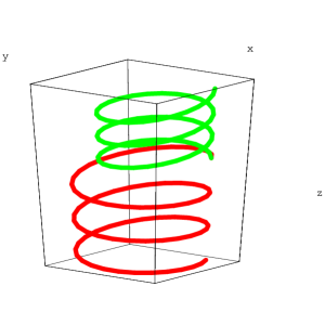
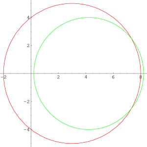
Figure 11: In the first picture we see two geodesics in three space, while in the second we see their projection onto the plane $xy$.

A more illuminating visualization of this three–dimensional geometry is provided by the picture of a congruence of geodesics. Given a point in this $3D$ space, we can consider all the geodesics that begin at that point and that have a radius $R$ falling in some interval:

$$R_{A}<R<R_{B}$$ (4.70)

Following each of them for some amount of parametric time $\lambda$ we generate a two dimensional surface. An example is given in fig.12.

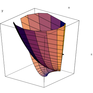
Figure 12: In this picture we present a congruence of geodesics for the space with $\Lambda=\Delta=\varpi=1$. All the curves start from the same point and are distinguished by the value of the radius $R$ in their circular projection onto the $xy$ plane.

The evolution of the universe can now be illustrated by its effect on a congruence of geodesics. Chosen a congruence like in fig.12, the shape of the surface generated by such a congruence depends on the value of the scale parameters $\Lambda$ and $\Delta$. We can follow the evolution of the congruence while the universe expands obtaining a movie. In fig.13 we present six photograms of such a movie:

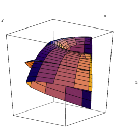
Figure 13: In this picture we present the same congruence of geodesics at six different times of the universe expansion, while $\Lambda$ grows and $\Delta$, after reaching a maximum, decreases.

Having illustrated the shape and the properties of the geodesics for the three dimensional sections of space–time we can now address the question of geodesics for the full space–time. To this effect we calculate first the three dimensional line element along the geodesics and we obtain the following result

$$\frac{d\ell^{2}\left(t,\lambda\right)}{d\lambda^{2}}\equiv\Lambda(t)\,\left[\,\dot{x}^{2}(\lambda)\,+\,\,\dot{y}^{2}(\lambda)\right]+\Delta(t)\,\left[\dot{z}(\lambda)+\frac{\varpi}{4}(x(\lambda)\,\dot{y}(\lambda)-y(\lambda)\,\dot{x}(\lambda))\right]^{2}=$$

$$=\frac{A_{1}^{2}}{96\Lambda(t)^{2}}\left(16\,R^{2}\,\Lambda(t)\,{\varpi}^{2}+\frac{{\left(-8\,\Lambda(t)+3\,\Delta(t)\,{\rho}^{2}\,{\varpi}^{2}+3\,R\,\Delta(t)\,\rho\,{\varpi}^{2}\,\cos(\theta-\varphi(\lambda))\right)}^{2}}{\Delta(t)}\right)\equiv$$

$$\equiv F^{2}(t,\varphi)\,\left(\frac{d\varphi}{d\lambda}\right)^{2}$$ (4.71)

In the last step of eq.(4.71) we have introduced the notation:

$$F^{2}(t,\varphi)\,=\,\left(R^{2}\,\Lambda(t)+\frac{{\left(-8\,\Lambda(t)+3\,\Delta(t)\,{\rho}^{2}\,{\varpi}^{2}+3\,R\,\Delta(t)\,\rho\,{\varpi}^{2}\,\cos(\theta-\varphi(\lambda))\right)}^{2}}{16\,\varpi^{2}\Delta(t)}\right)$$ (4.72)

and we have used relation (4.67).

Hence we obtain the complete space–time geodesics from those of three–space by solving the following equation that relates the time coordinate $t$ to the angular coordinate $\varphi$:

$$-A(t)\,\left(\frac{dt}{d\varphi}\right)^{2}+F^{2}(t,\varphi)=k\,\frac{4}{\varpi^{2}}\,\frac{A_{1}}{\Lambda^{2}(t)}\quad;\quad\left\{\begin{array}[]{cccl}k&=&-1&\mbox{time--like}\\ k&=&0&\mbox{null--like}\\ k&=&1&\mbox{space--like}\end{array}\right.$$ (4.73)

Furthermore, the constant $A_{1}$ is inessential and can always be fixed to $1$ since it can be traded for the constant $A_{2}$ which does not appear in the equation. The differential eq.(4.73) appears rather involved since $F^{2}(t,\varphi)$ depends both on time and the angle $\varphi$. Yet we can take advantage of the homogeneous character of our space–time and simplify the problem very much. Indeed due to homogeneity it suffices to consider the geodesics whose projection in the $xy$ plane is a circle centered at the origin and of radius $R$. All other geodesics with center in some point $\{x_{0}\,,\,y_{0}\}$ can be obtained from these ones by a suitable isometry that takes $\{0,0\}$ into $\{x_{0}\,,\,y_{0}\}$. So let us consider geodesics centered at the origin of the $xy$ plane. This corresponds to setting $\rho=0$. In this case we obtain:

$$F^{2}(t,\varphi)|_{\rho=0}\equiv F^{2}_{0}(t)\,=\,\frac{\Lambda(t)\,\left(4\,\Lambda(t)+R^{2}\,\Delta(t)\,{\varpi}^{2}\right)}{\Delta(t)\,{\varpi}^{2}}$$ (4.74)

which depends only on time and the geodesic equations are reduced to quadratures since we get:

$$\int_{0}^{\varphi_{max}}\,d\varphi=\int_{-\infty}^{t_{0}}\frac{\sqrt{A(t)}}{\sqrt{F^{2}(t)-\frac{4\,k}{\varpi^{2}\,\Lambda^{2}(t)}}}\,dt$$ (4.75)

The convergence or divergence of the second integral in eq.(4.75) determines whether or not there are particle horizons in the considered cosmology. Curiously, such horizons appear as an angular deficit. For each chosen radius $R$ one can explore the geodesic (which is a spiral) only up to some maximal angle $\varphi_{max}$ at each chosen instant of time.

4.3 Summarizing

Summarizing the above discussion we can say that each exact solution for a Bianchi type 2A cosmology, with or without matter, presents a typical feature which we can generically name a billiard feature. In lack of isotropy, the scale factors associated with the different dimensions (in this case we do not have cartesian dimensions, yet we can identify the notion of dimensions with the generators of the translation isometry algebra) undergo a quite different fate. Two dimensions grow indefinitely as in a isotropic big bang model, while the third expands to a maximum, then it contracts and tends to zero. The parameter governing this bending is $\varpi$, namely the only non vanishing structure constant that deforms the Heisenberg algebra away from an abelian algebra. An indication that this behaviour is related to branes is evident in the example of the space $0$–brane solution. There we observe that the direction which undergoes the billiard phenomenon is the direction in which lies the vector field, namely the $1$–form $A$, while those which expand indefinitely are the transverse ones. This is exactly the same as it was observed, for higher dimensions in paper [19]. There it was shown how the $\mathrm{A_{2}}$ solutions of the $E_{8(8)}/SO(16)$ sigma model could, in particular, be oxided to $D=10$ supergravity backgrounds containing $D3$–space branes. The dimensions of the brane underwent a maximum and then decayed to zero, while for the transverse ones the opposite was true. They were depressed at the moment the brane dimensions were enlarged and then expanded again while the parallel ones contracted. In this section we have examined the geometric and physical implications of this peculiar behaviour of the scale factors and we have explored the structure of the canonical metric representative of $A_{2}$ models. From the analysis of the previous sections, we know that these peculiar Heisenberg algebra cosmologies are dual to any other $A_{2}$ solution, since there is just one Weyl orbit of $\mathrm{A_{2}}$ embeddings.

5 Conclusions and Perspectives

In the present paper we have explored the structure of Weyl orbits for the embedding of regular subalgebras $\mathbf{G}_{r}\hookrightarrow\mathrm{E_{8(8)}}$. The relevance of this algebraic construction is that regular subalgebras of $\mathrm{E_{8(8)}}$ generate exact time dependent solutions of the sigma model $\mathrm{E_{8(8)}/SO(16)}$ and their embeddings determine the oxidation of such solutions to exact time dependent solutions of supergravity in ten dimensions. In particular we have considered the Weyl orbits of $\mathrm{A_{r}}$ subalgebras and we have shown that there is only one orbit up to $r=6$. In a future publication we plan to study the embeddings of other chains of subalgebras, for instance the $\mathrm{D_{r}}$ chain. The algebraic setup has been completely fixed here. For the $\mathrm{A_{r}}$ chain we have shown that in the unique Weyl orbit there is always a canonical representative that corresponds to a pure metric configuration in dimension $d=3+r$. For the $\mathrm{A_{2}}$ case the canonical metric representative is related to Bianchi type 2A homogeneous cosmologies based on the Heisenberg algebra. Through this relation we were able to present some new exact solutions of matter coupled Einstein theory in this Bianchi class that, up to our knowledge, were so far undiscovered. We made an extensive analysis of their geometrical properties and of their behaviour.

As we already pointed out in the previous paper [19], there are three main directions to be explored in connection with the present new developments. The first is the extension of our analysis to affine and hyperbolic algebras. This means first reduce to dimensions $D=1+1$ or $D=1+0$ and then oxide back to $D=10$. In this process new classes of solutions can be discovered, that include and extend the Geroch group. The second line of investigation is the application of our algebraic technique of deriving solutions to other low parameter cases, for instance the dependence on light–like coordinates, leading to the classification of gravitational waves. The third line of investigation is the microscopic interpretation of these classical supergravity solutions in terms of time–dependent boundary states and space–branes. To this effect, as we explained in the introduction, a firm control on the structure of Weyl orbits is particularly vital. Indeed it allows to duality rotate classical solutions to others that have a clear $D$–brane description.

We plan to address all these questions in next coming future publications.

References

[1]
S. Kachru, R. Kallosh, A. Linde, J. Maldacena, L. McAllister and
S. P. Trivedi, Towards inflation in string theory,
[arXiv:hep-th/0308055].
[2]
S. Kachru, R. Kallosh, A. Linde and S. P. Trivedi, De Sitter
vacua in string theory Phys. Rev. D 68 (2003) 046005
[arXiv:hep-th/0301240].
[3]
P. Fre, M. Trigiante and A. Van Proeyen, Stable de Sitter
vacua from N = 2 supergravity, Class. Quant. Grav. 19
(2002) 4167 [arXiv:hep-th/0205119];
M. de Roo, D. B. Westra, S. Panda and M. Trigiante,
Potential and mass-matrix in gauged N = 4 supergravity,
JHEP 0311 (2003) 022 [arXiv:hep-th/0310187].
[4]
M. Gutperle and A. Strominger, Spacelike branes, JHEP 0204 (2002) 018 [arXiv:hep-th/0202210].
[5]V. D. Ivashchuk and V. N. Melnikov, Multidimensional
classical and quantum cosmology with intersecting p-branes, J. Math. Phys. 39 (1998) 2866 [arXiv:hep-th/9708157];
[6]L. Cornalba, M. S. Costa and C. Kounnas, A resolution of the
cosmological singularity with orientifolds, Nucl. Phys. B 637 (2002) 378 [arXiv:hep-th/0204261];
L. Cornalba and M. S. Costa, On the classical stability of
orientifold cosmologies, Class. Quant. Grav. 20 (2003)
3969 [arXiv:hep-th/0302137].
[7]
G. Papadopoulos, J. G. Russo and A. A. Tseytlin, Solvable
model of strings in a time-dependent plane-wave background,
Class. Quant. Grav. 20 (2003) 969
[arXiv:hep-th/0211289].
[8] F. Quevedo, Lectures on string / brane
cosmology, [arXiv:hep-th/0210292].
[9] M. Gasperini and G. Veneziano, The pre-big bang scenario
in string cosmology, [arXiv:hep-th/0207130].
[10] B. Craps, D. Kutasov and G. Rajesh, String
propagation in the presence of cosmological singularities, JHEP
0206, 053 (2002) [arXiv:hep-th/0205101].
[11] T. Banks and W. Fischler, M-theory observables for
cosmological space-times, [arXiv:hep-th/0102077].
[12] J. Khoury, B. A. Ovrut, N. Seiberg, P. J. Steinhardt and
N. Turok, From big crunch to big bang, Phys. Rev. D 65, 086007 (2002) [arXiv:hep-th/0108187].
[13]
J. E. Lidsey, D. Wands and E. J. Copeland, Superstring
cosmology, Phys. Rept. 337, 343 (2000)
[arXiv:hep-th/9909061].
[14] A. E. Lawrence and E. J. Martinec, String field theory
in curved spacetime and the resolution of spacelike
singularities, Class. Quant. Grav. 13, 63 (1996)
[arXiv:hep-th/9509149].
[15]
A. Sen, Time evolution in open string theory JHEP 0210 (2002) 003 [arXiv:hep-th/0207105].
[16]
A. Sen, Rolling tachyon, JHEP 0204 (2002) 048
[arXiv:hep-th/0203211].
[17] Riess A G et al. 1998 Astron. J.1161009, Perlmutter S et al. 1999 Astron. J.517 565,
Sievers J L et al. 2002 Preprint
[arXiv:astro-ph/0205387]
[18] Linde A D 1990 Particle Physics and Inflationary Cosmology
(Switzerland: Harwood Academic)
[19] P. Fre, V. Gili, F. Gargiulo, A. Sorin, K. Rulik and M. Trigiante,
Cosmological backgrounds of superstring theory and solvable
algebras: Oxidation and branes, [arXiv:hep-th/0309237].
[20]V. D. Ivashchuk and V. N. Melnikov,
Billiard representation for multidimensional cosmology with
intersecting p-branes near the singularity, J. Math. Phys. 41 (2000) 6341 [arXiv:hep-th/9904077].
[21] T. Damour, M. Henneaux and H. Nicolai,
Cosmological billiards,
Class. Quant. Grav. 20 (2003) R145
[arXiv:hep-th/0212256].
[22]
M. Henneaux and B. Julia,
Hyperbolic billiards of pure D = 4 supergravities,
JHEP 0305 (2003) 047
[arXiv:hep-th/0304233].
[23]
S. de Buyl, G. Pinardi and C. Schomblond, Einstein billiards
and spatially homogeneous cosmological models,
[arXiv:hep-th/0306280].
[24]
T. Damour, M. Henneaux, A. D. Rendall and M. Weaver,
Kasner-like behaviour for subcritical Einstein-matter systems,
Annales Henri Poincare 3 (2002) 1049
[arXiv:gr-qc/0202069].
[25]
T. Damour and M. Henneaux,
Chaos In Superstring Cosmology,
Gen. Rel. Grav. 32 (2000) 2339.
[26]
T. Damour, M. Henneaux, B. Julia and H. Nicolai,
Hyperbolic Kac-Moody algebras and chaos in Kaluza-Klein models,
Phys. Lett. B 509 (2001) 323
[arXiv:hep-th/0103094].
[27]
T. Damour and M. Henneaux,
E(10), BE(10) and arithmetical chaos in superstring cosmology,
Phys. Rev. Lett. 86 (2001) 4749
[arXiv:hep-th/0012172].
[28]
T. Damour and M. Henneaux,
Oscillatory behaviour in homogeneous string cosmology models,
Phys. Lett. B 488 (2000) 108
[Erratum-ibid. B 491 (2000) 377]
[arXiv:hep-th/0006171].
[29]
T. Damour and M. Henneaux,
Chaos in superstring cosmology,
Phys. Rev. Lett. 85 (2000) 920
[arXiv:hep-th/0003139].
[30]
J. Demaret, Y. De Rop and M. Henneaux,
Chaos In Nondiagonal Spatially Homogeneous Cosmological Models In Space-Time Dimensions ¡= 10,
Phys. Lett. B 211 (1988) 37.
[31]
M. Bertolini, M. Trigiante and P. Fre, N = 8 BPS black holes
preserving 1/8 supersymmetry, Class. Quant. Grav. 16
(1999) 1519 [arXiv:hep-th/9811251];
M. Bertolini and M. Trigiante, Regular R-R and NS-NS BPS
black holes, Int. J. Mod. Phys. A 15 (2000) 5017
[arXiv:hep-th/9910237];
M. Bertolini and M. Trigiante, Regular BPS black holes:
Macroscopic and microscopic description of the generating
solution, Nucl. Phys. B 582 (2000) 393
[arXiv:hep-th/0002191];
M. Bertolini and M. Trigiante, Microscopic entropy of the
most general four-dimensional BPS black hole, JHEP 0010
(2000) 002 [arXiv:hep-th/0008201].
[32] L. Bianchi, Sugli spazi a tre dimensioni che ammettono un gruppo continuo
di movimenti, Memorie di Matematica e di Fisica della Societá
Italiana delle Scienze, Serie Terza 11 (1898) 267-352.
[33] H. Lü, C.N. Pope, K. Stelle Weyl Group Invariance and p-brane multiplets,
Nucl. Phys. B 476 (1996) 89
[arXiv:hep-th/9602140].
[34]L. Andrianopoli, R. D’Auria, S. Ferrara, P. Fre and M. Trigiante,
R-R scalars, U-duality and solvable Lie algebras, Nucl. Phys. B 496 (1997) 617 [arXiv:hep-th/9611014];
L. Andrianopoli, R. D’Auria, S. Ferrara, P. Fre, R. Minasian and
M. Trigiante, Solvable Lie algebras in type IIA, type IIB
and M theories, Nucl. Phys. B 493 (1997) 249
[arXiv:hep-th/9612202];
E. Cremmer, B. Julia, H. Lu and C. N. Pope, Dualisation of
dualities. I, Nucl. Phys. B 523 (1998) 73
[arXiv:hep-th/9710119].
[35] R.M. Wald, Phys. Rev. D28 (1983) 2118;
A A. Coley and J. Wainwright Class. Quantum Grav. 9 (1992)
651; M. Goliath and G. F. R. Ellis, Homogeneous cosmologies
with cosmological constant, Phys. Rev. D 60 (1999) 023502
[arXiv:gr-qc/9811068];
U. S. Nilsson and C. Uggla, Stationary Bianchi type II
perfect fluid models, [arXiv:gr-qc/9702039].
[36] J. Humprey, Reflection groups and Coxeter
groups Cambridge University Press 1990.